User's Guide to Income Imputation in the CE July 31, 2018

US Department Of Labor Bureau of Labor Statistics

Division of Consumer Expenditure Surveys

Bureau of Labor Statistics

Consumer Expenditure Survey Authors: Geoffrey Paulin, DCES Sally Reyes-Morales, SMD Jonathan Fisher, DPINR Initial Version: 12/13/2005 First Update: 12/01/2006 Second Update (Current Version): 7/31/2018

Multiple Imputation Manual:

Supplement to Consumer Expenditure Surveys Public Use Microdata Documentation (2004 onward)

I. BACKGROUND.

The purpose of this manual is to provide instructions to users regarding the proper use of multiply imputed data to draw statistically valid inferences in their works. Therefore, the main portion of this text describes application and usage of multiply imputed data, rather than its production or its statistical properties and derivations. However, for data users who are interested in better understanding them, detailed descriptions of the theoretical underpinnings of this process are documented elsewhere.1

A. Introduction and Method Overview.

Starting with the publication of the 2004 data, the Consumer Expenditure Surveys (CE) include income data that have been produced using multiple imputation. The purpose of this procedure is to fill in blanks due to nonresponse (i.e., the respondent does not know or refuses to provide a value for a source of income received by the consumer unit2 or a member therein) in such a way that statistical inferences can be validly drawn from the data. The process preserves the mean of each source of income, and also yields variance estimates that take into account the uncertainty built into the data from the fact that some observations are imputed, rather than reported. In some cases, respondents provide imprecise information regarding income. That is, when the respondent does not provide the exact value of a source for which receipt is reported, the interviewer asks the respondent to select from a list of possibilities the range in which the income falls. This range is known as a “bracket,” and the respondent is a “bracket reporter.” In such cases, five different values within the bracket are imputed according to an algorithm that is designed to preserve the mean. That is, the larger the number of imputations made through this method, the closer the mean of the imputations would converge to the mean of income observed by those respondents who reported actual values that fell within the bracket of interest.

When no value (precise or bracket) is reported for a particular source of income for which receipt is reported, the method used to derive the multiple imputations is regression-based. Essentially, a regression 1 Rubin, Donald B. Multiple Imputation for Nonresponse in Surveys (New York: John Wiley and Sons, Inc., 1987). 2 Similar to a “family” or “household.” According to the CE glossary, a “consumer unit comprises either: (1) all members of a particular household who are related by blood, marriage, adoption, or other legal arrangements; (2) a person living alone or sharing a household with others or living as a roomer in a private home or lodging house or in permanent living quarters in a hotel or motel, but who is financially independent; or (3) two or more persons living together who use their income to make joint expenditure decisions. Financial independence is determined by the three major expense categories: Housing, food, and other living expenses. To be considered financially independent, at least two of the three major expense categories have to be provided entirely, or in part, by the respondent.” (https://www.bls.gov/cex/csxgloss.htm)

2

is run to provide coefficients for use in estimating values for missing data points. The coefficients are then “shocked” by adding random noise to each, and missing values are estimated using the shocked coefficients. To each of these estimated values, additional random noise is added, to ensure that consumer units (or members) with identical characteristics (e.g., urban service workers aged 25 to 34) will not receive identical estimates for their income. The resulting values are used to fill in invalid blanks where they occur (i.e., due to nonresponse), while reported values are retained. This process is then repeated four times, so that a total of five imputed values are computed for each missing value. In addition, for the small number of cases in which the respondent does not report receipt of any source of income collected either at the member or consumer unit level, receipt of each source is imputed using logistic regression. In each case where receipt is imputed, the income value is treated as a missing data point, and is imputed using the method described above.

B. Historical Income Data Differences and Guidelines for use of Imputed Data.

Starting with the publication of the 1972-73 data, the CE introduced the concept of the “complete income reporter.” In general, consumer units are defined as complete income reporters if their respondents provide values for at least one of the major sources of income, such as wages and salaries, self-employment income, and Social Security income for their reference person (i.e., the first person named when the respondent is asked who is responsible for owning or renting their home). However, even complete income reporters may not have provided a full accounting of all sources of income. The first difference, therefore, between the data previously published and those available starting in 2004 is that the imputed data have all invalid missing values filled in, so that estimates using income can be generated for all consumer units, not only for complete income reporters.

In addition, the collected data contain only one observation of each income value for each consumer unit or member for whom a value is reported. The imputed data include five estimates of each observation, plus one additional estimate representing the mean of all five estimates. For example, when examining the collected data for a subset of interest (say, 100 particular consumer units who all report receipt of INTRDVX3), there is one column of data identifying the selected consumer units (i.e., 100 observations of NEWID4) and one column of data containing the associated income values of interest and dividends (i.e., 100 observations of INTRDVX). However, with the imputed data, there are five columns of income data (each containing 100 observations), each of which has a different value for income if the original value (INTRDVX) is missing due to an invalid nonresponse, or the same value as the original value, if the original value is provided by the respondent. In addition, there is a sixth column of income data (also containing 100 observations) that contains the mean of the five columns of data just described.

Based on the information presented so far, some readers may conclude that it does not matter which column is used in data analysis, so it is reasonable to select one of the five imputed columns randomly and use it to draw inferences, or simply to use the sixth column provided in the CE microdata files (i.e., the column of the means, described subsequently) for these purposes. However, using one column of data in this way does not adequately capture the uncertainty built into the data by the very nature that some of it has been imputed rather than collected from the respondent. Therefore, at a minimum, variance estimates obtained from using one column of data will be biased. Proper variance estimation requires use of the five columns of imputed data. Similarly, proper calculation of the estimated mean requires averaging the estimates from all five columns of data. However, it can be shown that finding the average of the 500 observations (that is, the five columns of imputed data for each of the 100 consumer units selected for examination) yields the same answer as averaging each of the five imputations to get one column of 100 imputed means, and then finding 3 Interest and dividend income. For more information regarding this and other variable names, see the table in section I.C., “Variable Names (2013 onward).” 4 The unique identifier associated with each consumer unit in a particular quarter of data. Details are available in the Interview and Diary Survey data dictionaries to which this document is supplementary. To access these dictionaries, other related documents, and CE microdata, see https://www.bls.gov/cex/pumd_doc.htm.

3

the mean of the 100 observations. (See II.A., “Computing Means.”) Therefore, the sixth column is included as a convenience for users who are interested only in calculating means. Regardless, it is not recommended that users who want to compute variances, regression parameters, or other statistical results use only the sixth column in their analyses. C. Variable Names (2013 onward).

Imputed income data appear on both the MEMi and FMLi files of both the Interview and Diary Surveys.5 While the names of some of the variables differ across the surveys, their definitions are the same (e.g., SALARYX in Interview and WAGEX in Diary). For convenience, the Interview Survey variables are used in the examples in this document. Starting in the second quarter of 2013, the names of the income variables as they are used in the Interview Survey, both reported and imputed, are as follows, in the order they appear in CE publications:6

Income

Variable:

Reported,

MEMI File,

Interview

Survey Variable Description

Associated 5 imputed income

variables Mean imputed income variable

SALARYX During the past 12 months, what was the amount of wages or salary income received, before any deductions?

SALARYX1 - SALARYX5 SALARYXM = mean(SALARYX1 - SALARYX5)

SEMPFRMX What was the amount of self-employment income or loss?

SEMPFRM1 - SEMPFRM5 SEMPFRMM = mean(SEMPFRM1 - SEMPFRM5)

RRRETIRX Amount of last Social Security or Railroad Retirement check

RRRETIR1 - RRRETIR5 RRRETIRM = mean(RRRETIR1 - RRRETIR5)

SOCRRX Annual amount of Social Security and Railroad Retirement income received by member in past 12 months

SOCRRX1 – SOCRRX5 SOCRRM = mean(SOCRRX1 – SOCRRX5)

SSIX Amount received in supplemental security income checks combined

SSIX1 - SSIX5 SSIXM = mean(SSIX1 - SSIX5)

Income

Variable:

Reported, FMLI

File, Interview

Survey Variable Description

Associated 5 imputed income

variables Mean imputed income variable

RETSURVX What was the amount received in retirement, survivor, or disability pensions during the past 12 months?

RETSURV1- RETSURV5 RETSURVM = mean(RETSURV1- RETSURV5)

INTRDVX Amount of income received from interest and dividends

INTRDVX1- INTRDVX5 INTRDVXM = mean(INTRDVX1- INTRDVX5)

5 In this case, i is “I” for Interview data, and “D” for Diary data. For information about the MEMi and FMLi files, see the main documentation that this manual supplements (https://www.bls.gov/cex/pumd_doc.htm); for example, “Getting Started with Consumer Expenditure Survey (CE) Public-Use Microdata (PUMD)” version 3.0, August 29, 2017 (https://www.bls.gov/cex/pumd_novice_guide.pdf), and “2016 Users’ Documentation, Interview Survey, Public-Use Microdata (PUMD), Consumer Expenditure,” August 29, 2017 (https://www.bls.gov/cex/2016/csxintvw.pdf). 6 The income sections of the survey instruments for Interview and Diary were substantially revised in 2013, with changes effective as of April 1 (i.e., second quarter) for the Interview, and January 1 (i.e., first quarter) for the Diary. Some variables were renamed (e.g., PENSIONX became RETSURVX), combined (e.g., ALIOTHX, CHDOTHX, UNEMPLX, and COMPENSX became OTHREGX) or otherwise rearranged (e.g., dividends were split from FININCX and combined with INTERESTX, resulting in ROYESTX and INTRDVX). The list of variable names effective from 2004 through the first quarter of 2013 are included in the appendix to this document.

4

Income

Variable:

Reported, FMLI

File, Interview

Survey Variable Description

Associated 5 imputed income

variables Mean imputed income variable

ROYESTX Amount of income received from royalty income or income from estates and trusts

ROYESTX1- ROYESTX5 ROYESTXM = mean(ROYESTX1- ROYESTX5)

NETRENTX What was the amount of net rental income or loss?

NETRNTX1- NETRNTX5 NETRNTXM = mean(NETRNTX1- NETRNTX5)

OTHREGX Amount of income received from any other source such as Veteran’s Administration (VA) payments, unemployment compensation, child support, or alimony

OTHREGX1- OTHREGX5 OTHREGXM = mean(OTHREGX1- OTHREGX5)

WELFAREX Amount received from public assistance or welfare including money received from job training grants such as Job Corps

WELFARE1- WELFARE5 WELFAREM = mean(WELFARE1- WELFARE5)

OTHRINCX Amount received in other money income including money received from care of foster children, cash scholarships and fellowships, or stipends not based on working

OTHRINC1- OTHRINC5 OTHRINCM = mean(OTHRINC1- OTHRINC5)

FS_AMT What was the dollar value of the last food stamps or EBT received?

FS_AMT1-FS_AMT5 FS_AMTM = mean(FS_AMT1-FS_AMT5)

FINCBTAX* Total amount of family income before taxes in the last 12 months

FINCBTX1- FINCBTX5 FINCBTXM = mean(FINCBTX1- FINCBTX5)

FINATXEn* (Computed)

Total amount of family income after taxes in the last 12 months, derived from imputed data only

FINATXE1- FINATEX5 FINATXEM = mean(FINATXE1- FINATXE5)

FSALARYX* Total amount of income received from salary or wages before deduction by family grouping; FSALARYX= Sum SALARYX + SALARYBX** for all consumer unit members

FSALARY1-FSALARY5 FSALARYM = mean(FSALARY1-FSALARY5)

FSMPFRMX* Total amount of income received from self-employment income by family grouping; FSMPFRX= Sum SEMPFRMX + SMPFRMBX** for all consumer unit members

FSMPFR1-FSMPFR5 FSMPFRM = mean(FSMPFR1-FSMPFR5)

FRRETIRX* Total amount received from Social Security benefits and Railroad Benefit checks prior to deductions for medical insurance and Medicare; FRRETIRX= Sum SOCRRX for all consumer unit members

FRRETIR1-FRRETIR5 FRRETIRM = mean(FRRETIR1-FRRETIR5)

FSSIX* Amount of Supplemental Security Income from all sources received by all consumer unit members in past 12 months; FSSIX = (sum SSIX + SSIBX** from MEMI file for all consumer unit members)

FSSIX1-FSSIX5 FSSIXM = mean(FSSIX1-FSSIX5)

* Summary variable created from MEMI file data. FINCBTAX and FINATXEn also include FMLI file data. See appendix for more about FINATXEn (income after taxes). ** The “BX” suffix indicates that the variable was the result of a bracket report. See “Data dictionary beginning 1996 in the CE Public-use Microdata (PUMD),” https://www.bls.gov/cex/pumd/ce_pumd_interview_diary_dictionary.xlsx). D. Other Related Variables.

Additional variables are also available that are created from, or related to, the imputed income variables. These include INC_RNKn and various descriptor variables (section D2. below), which describe the reason for imputation. D1. INC_RNKn. As described in the CE public use microdata dictionary, INC_RANK is created using complete income reporters only. They are sorted in ascending order of reported income before taxes (FINCBTAX), and

5

ranked according to a weighted population rank, so that quintiles and other distributional measures can be obtained. For the imputed data, INC_RNK1 through INC_RNK5 and INC_RNKM are also created in a similar way. The difference is that they each use all consumer units, instead of complete reporters only, and that they are based on sorts of FINCBTXn. (That is, INC_RNK1 is derived from FINCBTX1, etc.) D2. Descriptor Variables. Imputation descriptor variables are coded to describe whether the income variable has undergone multiple imputation, and if so, for what reason. The imputation descriptor variable for each income variable is defined in the following tables. MEMBER INCOME VARIABLES

Income

variable name

Associated imputation

descriptor variable

SALARYX SALARYXI

SEMPFRMX SEMPFRMI

RRRETIRX RRRETIRI

SOCRRX N/A*

SSIX SSIXI *SOCRRX is used to compute RRRETIRX and has no associated imputation descriptor variable of its own. FMLI INCOME VARIABLES

Income

variable name

Associated imputation

descriptor variable

RETSURVX RETSURVI INTRDVX INTRDVXI ROYESTX ROYESTXI NETRENTX NETRENTI OTHREGX OTHREGXI WELFAREX WELFAREI OTHRINCX OTHRINCI FS_AMT FS_AMTXI

FMLI SUMMARY INCOME VARIABLES*

Summary income

variable

Associated imputation

descriptor variable

FINCBTAX FINCBTXI

FSALARYX FSALARYI

FSMPFRMX FSMPFRXI

FRRETIRX FRRETIRI

FSSIX FSSIXI * These represent the sum of the member-level income variables for each family.

6

Each descriptor variable has a numeric value three characters in length. There are no blanks or blank codes (such as “A”, “D” or “T”) for descriptor variables. The descriptor variables are defined as follows:

CODE VALUE CODE DESCRIPTION

100* no multiple imputation – reported income is a valid value, or valid blank7 201 multiple imputation due to invalid blank only 301 multiple imputation due to bracketing only 501 multiple imputation due to conversion of a valid blank to an invalid blank

(occurs only when reported values for all sources of income—MEMI and FMLI—for the consumer unit were valid blanks)

* Note that when no imputation occurs, the assigned code value is 100 at both the individual source level and at the summary level.

Description of code values for Summary FMLI Income imputation descriptor variables

CODE VALUE CODE DESCRIPTION

100 No imputation. This would be the case only if NONE of the variables that are summed to get the summary variables is imputed.

2nn Imputation due to invalid blanks only. This would be the case if there are no bracketed responses, and at least one value is imputed because of invalid blanks.

3nn Imputation due to brackets only. This would be the case if there are no invalid blanks, and there is at least 1 bracketed response

4nn Imputation due to invalid blanks AND bracketing. 5nn Imputation due to conversion of valid blanks to invalid blanks. (Occurs only

when initial values for all sources of income for the consumer unit and each member are valid blanks.)

Definition of nn: The “nn” is the count of the number of members in the consumer unit who have imputed data (whether due to invalid blanks, brackets, or both).

E. Topcoding Income Imputation.

The five income imputations and mean column are all subject to topcoding rules described in the public-use microdata documentation.8 One critical value is determined for all five imputations and the mean column. If any of the imputations (INCOME1-INCOME5) for a particular member of the consumer unit fall above the upper critical value (for positive numbers) or below the lower critical value (for negative numbers), then each imputed value (INCOME1-INCOME5) is topcoded for that record, and the associated flag will be coded as “T”. Additionally, the mean value (INCOMEM) is topcoded and the flag will also be given a value of “T'”.

7 Income values are collected in two steps. First, the respondent is asked whether anyone in the consumer unit has received income from a particular source. Then, if yes, the amount received is requested. However, if no, the amount received is recorded as a “valid blank,” rather than as $0. For income sources (except summary variables) recorded in the FMLi files, the value is collected for the consumer unit as a whole, if receipt is reported. For income sources recorded in the MEMBi files, the value is collected for each member of the consumer unit who is at least 14 years old. 8 See “Protection of Respondent Confidentiality,” available at: https://www.bls.gov/cex/pumd_disclosure.htm; and “2016 Topcoding and Suppression, INTERVIEW SURVEY AND DIARY SURVEY, CONSUMER EXPENDITURE PUBLIC USE MICRODATA,” August 29, 2017, available at: https://www.bls.gov/cex/pumd/2016/topcoding_and_suppression.pdf.

7

II. Applications.

A. Computing Means.

A1. Unweighted means.

As noted in the text, the mean income for a group of interest can be calculated by summing all data observations for the five imputations, and dividing by the total number of observations. Mathematically, the formula that applies is:

where X is the value of income, n is the number of rows, and m is the number of columns.

As an applied example, consider the following: INTRDVX INTRDVX1 INTRDVX2 INTRDVX3 INTRDVX4 INTRDVX5 100 100 100 100 100 100 D 50 250 300 20 80 In this example, the first consumer unit has reported a value for INTRDVX ($100), but the second consumer unit has only reported receipt of this income source. However, values (INTRDVX1 through INTRDVX5) are imputed for this consumer unit.

To find the mean value for the complete data set (i.e., the collected data and the imputed data), sum each imputed observation (100 + 100 + … + 100 + 50 + …. + 20 + 80) and divide the resulting total (1,200) by the total number of observations (n*m=2*5=10) to get a mean value of 120. Or, following the formula above:

Sum each row within each column (100+50=150; 100+250=350; etc.) and then sum the five sums (150+350+…+180 = 1,200) and divide by 10 (n*m=10, as shown above), and the mean is 120. However, the same value results when the mean of each row is calculated, and the mean of those means is then found. Using the same example, the data would now appear as follows: INTRDVX1 INTRDVX2 INTRDVX3 INTRDVX4 INTRDVX5 INTRDVXM 100 100 100 100 100 100 50 250 300 20 80 140 Adding the two means (100+140) yields a total of 240. Dividing this by the number of means added (2) yields 120, the same value as obtained by finding the mean of all 10 observations. A2. Weighted means. In order to calculate the weighted mean without including variance calculations, the process using the complete data set is also straightforward. The weighted mean for the sixth column of data (INTRDVXM in this example) is calculated using the appropriate data weighting method described in the main text for

)/()(1 1

mnXm

j

n

iij

)/()(1 1

mnXm

j

n

iij

8

which this documentation serves as supplement.9 The result is the weighted mean for this group. Specifically, suppose that the first consumer unit represents 5,000 similar units in the U.S. population, and the second consumer unit represents 7,500. In these circumstances, FINLTWT21 is 5,000 for the first consumer unit and 7,500 for the second unit. The weighted mean is: [(100*5,000) + (140*7,500)]/(5,000 + 7,500) or 124.

When variances are to be calculated, as described in the next section, it is recommended that the mean be found by calculating the mean of each of the five columns containing imputed data (that is, INTRDVX1 through INTRDVX5), and then averaging these means. Nevertheless, the mean will be the same, as demonstrated above for unweighted means. Following this procedure, the weighted means for each column are:

INTRDVX1 INTRDVX2 INTRDVX3 INTRDVX4 INTRDVX5

70 190 220 52 88

and the mean of these observations (70, 190, 220, 52, and 88) is 124.

B. Computing Variances.

When using multiply imputed data, the proper variance computation is straightforward, but involves more steps than the computation of variance from data sets in which no observations are initially missing. The reason is that in the latter case, all information is known. However, when data are imputed, there is additional uncertainty added to the complete data set by the very fact that the imputed data are estimates of values, rather than collected values. With multiple imputation, this imputation-related uncertainty is incorporated into the variance term, because more than one estimate of each missing value is posited. The proper variance is composed, then, of three elements: the “within imputation variance,” which is the usual variance computed for each column of the completed data set; the “between imputation variance,” which accounts for variance across the columns of data; and an imputation adjustment factor described in Rubin (1987),10 to account for the fact that a finite number of columns of data are created in the imputation process. B1. Variances for Unweighted Means. Consider the example shown in section II.A1., “Unweighted means.” In this case, two hypothetical consumer units reporting receipt of INTRDVX are shown, one of which reports a value ($100) while the other has values imputed. The data shown are: INTRDVX INTRDVX1 INTRDVX2 INTRDVX3 INTRDVX4 INTRDVX5 100 100 100 100 100 100 D 50 250 300 20 80 The first step is to compute the mean of each column of completed data (INTRDVX1 through INTRDVX5). Using notation consistent with Rubin (1987), this is:

(1)

where is the nth observation of column i. In the current example, 1 <= i <= 5, and n = 2 for each column.

9 See, for example, “2016 Users’ Documentation, Interview Survey, Public-Use Microdata (PUMD), Consumer Expenditure,” August 29, 2017, pp. 30-31; https://www.bls.gov/cex/2016/csxintvw.pdf. 10 p. 84-91.

n

QQ

n

jij

i

1

*

*ˆ

ijQ*

9

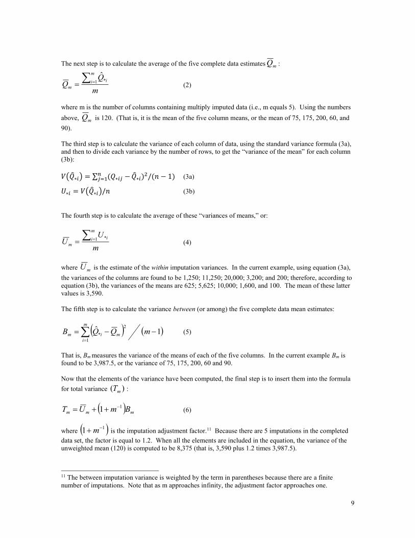
The next step is to calculate the average of the five complete data estimates :

(2)

where m is the number of columns containing multiply imputed data (i.e., m equals 5). Using the numbers above, is 120. (That is, it is the mean of the five column means, or the mean of 75, 175, 200, 60, and 90). The third step is to calculate the variance of each column of data, using the standard variance formula (3a), and then to divide each variance by the number of rows, to get the “variance of the mean” for each column (3b): 𝑉(�̂�∗𝑖) = ∑ (𝑄∗𝑖𝑗 −𝑛

𝑗=1 �̂�∗𝑖)2/(𝑛 − 1) (3a)

𝑈∗𝑖 = 𝑉(�̂�∗𝑖)/𝑛 (3b) The fourth step is to calculate the average of these “variances of means,” or:

(4)

where is the estimate of the within imputation variances. In the current example, using equation (3a), the variances of the columns are found to be 1,250; 11,250; 20,000; 3,200; and 200; therefore, according to equation (3b), the variances of the means are 625; 5,625; 10,000; 1,600, and 100. The mean of these latter values is 3,590. The fifth step is to calculate the variance between (or among) the five complete data mean estimates:

(5)

That is, Bm measures the variance of the means of each of the five columns. In the current example Bm is found to be 3,987.5, or the variance of 75, 175, 200, 60 and 90. Now that the elements of the variance have been computed, the final step is to insert them into the formula for total variance :

(6) where is the imputation adjustment factor.11 Because there are 5 imputations in the completed data set, the factor is equal to 1.2. When all the elements are included in the equation, the variance of the unweighted mean (120) is computed to be 8,375 (that is, 3,590 plus 1.2 times 3,987.5).

11 The between imputation variance is weighted by the term in parentheses because there are a finite number of imputations. Note that as m approaches infinity, the adjustment factor approaches one.

mQ

mQ

Qm

i im

1 *ˆ

mQ

mU

Um

i im

1 *

mU

m

imim mQQB

1

2

* 1ˆ

)( mT

mmm BmUT 11

11 m

10

B2. Variances for Weighted Means. When calculating the variance for the weighted mean, the procedure is similar to the procedure for unweighted means. In this case, the weighted mean is used instead of the unweighted mean where appropriate. That is, continuing to rely on the example from section II.A2., “Weighted means” (in which the first consumer unit represented 5,000 similar units and the second represented 7,500), it can be shown

that the five observations for each are 70, 190, 220, 52, and 88, and that equals 124. Computing

the variance of each is not easily shown, as it depends on the values of the 44 replicate weights (r).12 The method for computing these variances, though, is described in the main document to which this work is a supplement. That is, for each imputed column of income data,

The formula for computing is the same as described in the unweighted variance section (II.B1.), as is

the computation of its elements ( and ). Note that because each “Q” element of U*i is itself a mean, there is no need to divide any individual U*i further by anything else. That is, each U*i is treated as a variance of a mean before computing . C. Standard Error of the Mean (SE).

C1. Computation. Once the total variance ( ) is calculated, the standard error of the mean (SE) of the imputed data is

calculated as usual—that is, . Once obtained, the SE is used in the usual way in hypothesis testing. For example, the value can be used to compute a standard 95 percent confidence interval around the mean of the complete data set value of interest (that is, around ). However, the degrees of freedom associated with the t-value used in this computation are calculated according to special formulas described subsequently. See “Use in Hypothesis Testing,” below, for details. C2. Use in Hypothesis Testing. As noted above, the SE can be used in standard hypothesis testing. For example, a standard confidence interval can be built around using SE in the conventional way. According to Rubin (p.77), the formula

for the standard 100(1-)% interval estimate of is:

“where is the upper 100/2 percentage point of the student t distribution on degrees of

freedom (e.g., if and , .”

12 The variance is computed through the method known as “balanced repeated replication”, or “BRR.” The names of the replicate weights (r, above) for CE data are WTREPnn, where “01”<=nn<=”44.”

iQ*ˆ

mQ

iQ*ˆ

44

12

Q̂*Q̂44

1=*Q̂V *

r iriiU i

mT

mU mB

mU

mT

mTSE

Q

QQ

21

)2/( mTtQ

2vt vv 95.1 96.12 vt

11

Note, though, that the value for degrees of freedom is calculated in a special way for imputed data. One method is applicable when the complete (i.e., post-imputation) dataset is “large.”13 According to Rubin (p. 77),

where is defined as the relative increase in variance due to nonresponse, and is computed according to the following formula:

.

In addition, Rubin (p. 77) provides the formula for computing an F-test in which is compared against a

null value of interest, :

“where is an random variable on one and degrees of freedom.” However, not all datasets are “large,” even when using CE data. For example, a researcher using CE data to study a distinct subset of the sample (e.g., consumers of a particular age, family type, and family size) might find that “large sample methods” are not applicable. In this case, there is another formula, provided by Barnard and Rubin (1999). In that article, the authors distinguish between vcom, the “complete-data degrees of freedom,” vm, the “calculated repeated-imputation degrees of freedom” just described—denoted herein as “v” for consistency with notation used throughout this document, and an “adjusted degrees of freedom,” or �̃�𝑚, which “is always less than or equal to vcom; and … [which] equals vm when vcom is infinite.”14 The formula is:

1

ˆ11~

obsm vv

v ,

where mcomcom

comobs v

vv

v ̂131ˆ

,

and

13 Barnard and Rubin (1999) state (p. 948) that “the size of the complete dataset is large, in the sense that, if there were no missing values, inferences would be based on large sample methods; i.e.[,] the degrees of freedom for standard errors and denominators of test statistics would effectively be set at infinity.” 14 See “SUMMARY,” p. 948.

2111 mrmv

mr

mmm UBmr 11

Q

0Q

mm TQQF 20,1Prob

,1F F v

mmm TBm /1ˆ 1

12

is approximately the Bayesian fraction of missing information for the unknown quantity of interest; is the complete-data degrees of freedom15 (i.e., n-1 for unweighted data, and 44 for weighted data). Once computed, the adjusted degrees of freedom are used in the same way as described above for “large” data sets. An obvious question arises: with “large” being a vague term, when is it appropriate to use the adjusted degrees of freedom instead of the unadjusted degrees of freedom? While Barnard and Rubin do no provide a specific example, they do state: “When vcom is small and there is only a modest proportion of missing data, the calculated repeated-imputation degrees of freedom, 𝑣𝑚, for the t reference distribution can be much larger than vcom, which is clearly inappropriate.”16 Therefore, it seems reasonable to compute the unadjusted degrees of freedom, and compare them to the observed degrees of freedom (i.e., sample size minus 1 for unweighted data). If the unadjusted degrees of freedom exceed the observed degrees of freedom, it is appropriate to use the adjusted degrees of freedom.17 C2a. Example: Computing a confidence interval Using the example from the unweighted means section (II.A1.), recall that equals 120, and Tm = 8,375. To compute the 95 percent confidence interval around this value, the formula described in section II.C2. (“Use in Hypothesis Testing”) applies. That is, using the unadjusted degrees of freedom,

where

𝑇𝑚

12⁄

= 𝑆𝐸 = √8,375 ≈ 91.5 To find , the degrees of freedom must be calculated. As described earlier, Bm equals 3,9875.5,

and equals 3,590. Using this information, is computed as follows: 𝑟𝑚 = (1 + 𝑚−1) 𝐵𝑚 �̅�𝑚⁄ = [1 + (5−1)] × (3,975.5 3,590⁄ ) ≈ 1.328858 15 As derived from Barnard and Rubin, equations (3) and (4) (p. 949), and (2) (p. 948). See SAS/STAT(R) 9.2 User's Guide, Second Edition, “The MIANALYZE PROCEDURE,” “Details: MIANALYZE Procedure,” “Combining Inferences from Imputed Data Sets,” last section of the page. Available at: https://support.sas.com/documentation/cdl/en/statug/63033/HTML/default/viewer.htm#statug_mianalyze_sect012.htm. 16 SUMMARY, p. 948. 17 This supposition is supported by the SAS PROC MIANALYZE documentation. It says: “When the complete-data degrees of freedom are small, and there is only a modest proportion of missing data, the computed degrees of freedom, , can be much larger than , which is inappropriate. For example, with

and , the computed degrees of freedom , which is inappropriate for data sets with complete-data degrees of freedom less than .” For clarification, the “r” in “ ” is the same rm defined in the text above as “the relative increase in variance due to nonresponse,” and denotes the same thing as vcom, just using different notation than Barnard and Rubin use. See SAS/STAT(R) 9.2 User's Guide, Second Edition, “The MIANALYZE PROCEDURE,” “Details: MIANALYZE Procedure,” “Combining Inferences from Imputed Data Sets,” last section of the page. Available at: https://support.sas.com/documentation/cdl/en/statug/63033/HTML/default/viewer.htm#statug_mianalyze_sect012.htm.

comv

Q

21

)2/( mTtQ

;120Q

)2/(tU mr

13

Thus, 𝑣 = (𝑚 − 1)(1 + 𝑟𝑚

−1)2 = (5 − 1)[1 + 1.328858−1]2 ≈ 12.285. The t-value for the 95 percent confidence level with 12 degrees of freedom is approximately 2.18. Therefore, the confidence interval is computed as follows: �̅� ± 𝑡𝑣(𝛼 2)𝑇𝑚

1/2⁄ = 120 ± (2.18 × 91.5) The resulting confidence interval is approximately: −79 ≤ �̅� ≤ 319 But note: The unadjusted degrees of freedom (12) is greater than the total number of observations in the complete data set (10), which is clearly inappropriate, according to Barnard and Rubin. The adjusted degrees of freedom in this case are derived as follows:

56962.0375,8/5.975,3)51(/)1(ˆ 11

mmm TBm

22785.343038.09)12/10()56962.01()110(3)110(1)110(ˆ1

31ˆ

mcom

com

comobs v

vv

v

and

556.222785.3

1285.121

ˆ11~

11

obsm vv

v

The adjusted degrees of freedom is less than 3, meaning that 𝑡�̃�𝑚

(𝛼/2) is between 3.182 (when 𝑡�̃�𝑚

(𝛼/2) = 3) and 4.303 (when 𝑡�̃�𝑚(𝛼/2) = 2). Using linear interpolation, 𝑡�̃�𝑚

(𝛼/2) is estimated to be about 3.680.18 Therefore, the confidence interval is: �̅� ± 𝑡�̃�𝑚

(𝛼 2)𝑇𝑚1/2⁄ = 120 ± (3.680 × 91.5)

and −217 ≤ �̅� ≤ 457 which is a much wider (and therefore more conservative) confidence interval. Note that linear interpolation is not necessary to demonstrate the wider confidence intervals. Whether the formula above is applied using

18 In a simple example, if the degrees of freedom were estimated to be 2.5, this would be half way between 2 and 3 degrees of freedom, and the t-value would be estimated to be half way between 4.303 and 3.182 and, or about 3.743. However, it is actually 55.6 percent of the way between 2 and 3 degrees of freedom. Therefore, the value is 55.6 percent of the way between 4.303 and 3.182, or ((3.182 – 4.303)*(0.556)) + 4.303 = 3.680. Another way to show this is to treat the t-values as functions of degrees of freedom, and compute the equation of the line segment according to the usual formula, y = mx +b, where y is the t-statistic, x is the degrees of freedom, m is the slope (change in y divided by change in x), and b is the intercept. In this case, the change in y is 1.121 (i.e., 4.303 – 3.182, as degrees of freedom goes from 2 to 3). Change in x is -1 (2 – 3). Therefore, m = -1.121. Since y = -1.121x + b, it is easy to find b by substituting one of the y and x sets into the formula. That is, 3.182 = -1.121*2 + b, or 3.182 = -2.242 + b. From this, b is found to be 6.545. Now, using this information to estimate the value of the t statistic when degrees of freedom is 2.556 is straightforward: y = -1.121*2.556 + 6.545, or y = 3.680, as shown before.

14

3 or 2 degrees of freedom, the confidence interval will be wider than when using 12 degrees of freedom, as done in the in the example using the unadjusted degrees of freedom estimate. C2b. Example: Conducting an F-test As described earlier, the F-test is used to compare to a null value. For example, suppose that the population reports average interest income of $150. To test whether or not the mean of the test sample ($120) is statistically significantly different from $150, the F-test is carried out as follows:

Prob {𝐹1,�̃�𝑚> (𝑄0 − �̅�𝑚)2 𝑇𝑚} Prob {𝐹1,3 > (150 − 120)2 8,375}⁄⁄

Prob{𝐹1,3 > 0.107} At the 95 percent confidence level, 𝐹1,3 = 10.13. Because 10.13 is greater than 0.107, the null hypothesis is not rejected. Note that the degrees of freedom are rounded up to 3 for the denominator from 2.556. If rounded to 2, the F statistic is even larger (𝐹1,2 = 18.52). Therefore, there is no need for linear interpolation. The null hypothesis is not rejected in either case (i.e., whether degrees of freedom are rounded to 2 or 3). D. Distributional Analyses using Imputed Income.

Currently, the Consumer Expenditure Survey publishes two types of standard table that describe income class: range (e.g., less than $15,000) and distribution (quintile and decile). Using these classifications, at least two different types of analysis can be performed: one where other characteristics are described as a function of, or related to, income; and one in which income distribution alone is of interest. An example of the first case is the current standard table publication. That is, these tables show how expenditures, age of reference person, and other characteristics differ across income classifications. An example of the second case is computation of the Lorenz curve or Gini coefficient for a particular group. (Examples of each follow.) The first method is used to produce the standard published tables, and is called the “publication method” throughout the remainder of this section. The second method is called the “distributional method.” D1. Publication Method. In the standard published tables, income is used as a classifier variable, and means for expenditures, age of reference person, and other variables are described by income class (for example, less than $15,000 or first income quintile or decile). With imputed income, the values in the “mean” column (i.e., the values for FINCBTXM) are used to classify consumer units by income group. This is because FINCBTXM represents the “best guess” of income for the consumer unit. As an example, suppose that the following observations are selected for study:19

19 These data are not actual imputed data. They are simulated by starting with $50,000 and adding or subtracting a random value between $0 and $49,999 to ensure all simulated values are between $1 and $99,999. Whether the random number is added or subtracted is also randomly determined.

Q

15

ConsumerUnit FINCBTX1 FINCBTX2 FINCBTX3 FINCBTX4 FINCBTX5 FINCBTXM

1 51,580 22,701 53,967 87,617 298 43,233 2 89,164 96,337 62,853 74,799 45,814 73,793 3 38,841 83,616 72,586 75,456 30,077 60,115 4 20,568 19,116 54,186 19,190 4,896 23,591 5 5,114 10,352 44,733 39,086 36,163 27,090 6 41,488 64,692 626 94,851 77,271 55,786 7 58,957 535 35,711 22,920 17,212 27,067 8 54,711 16,527 85,930 54,136 18,579 45,977 9 92,395 90,650 54,030 98,502 61,983 79,512

10 98,228 25,890 54,191 34,835 97,515 62,132 To compute means and variances for the $20,000 to $29,999 income group, consumer units 4, 5, and 7 are used. The unweighted mean income for this group is: (23,591 + 27,090 + 27,067)/3 = $25,916. To compute the variance (Tm) for this income group, the method described in the unweighted variance section (II.B1.) is used. That is, the variance U1 is calculated using the values from FINCBTX1 for this group (20,568; 5,114; and 58,957). Using the formulas described in the same section (II.B1.), the standard error of the mean for this group is $16,886. To compute weighted means and standard errors, these same consumer units and their appropriate weights would be used in the way described in the weighted variance computation section (II.B2.). D1a. Quintiles. Using these data, the mean and variance for each quintile can also be calculated. Because there are 10 observations shown here, each (unweighted) quintile is composed of two consumer units. To find the mean income for the first quintile, the data are sorted by FINCBTXM, and the first two consumer units (i.e., the first 20 percent in line) are selected for analysis. The resulting data set is:

Consumer Unit FINCBTX1 FINCBTX2 FINCBTX3 FINCBTX4 FINCBTX5 FINCBTXM

4 20,568 19,116 54,186 19,190 4,896 23,591 7 58,957 535 35,711 22,920 17,212 27,067

Mean income for this quintile is $25,329. The standard error of the mean for this quintile is $20,808. D1b. Regression. In regression analysis, it may be useful either to use income category as a binary variable, or to run separate regressions by income group. (For example, to calculate marginal propensity to consume food for the $20,000 to $29,999 group.) In these cases, the same classifications would be used as just described: that is, for consumer units 4, 5, and 7, the binary variable is equal to 1, and is equal to 0 for all other consumer units. If income is to be used as a continuous variable for the $20,000 to $29,999 group, then five regressions are run using FINCBTX1 through FINCBTX5 as described in the subsequent regression section (II.E.). D2. Distributional method.

At times, only mean income per group, and not variance, is needed. Two related applications of this case involve tools used in analysis of income distribution: The Lorenz curve and the Gini coefficient. (See section II.D3. for details.) To compute means by quintile in this case, each income variable (FINCBTX1 through FINCBTX5) is sorted by its associated INC_RNKn value (that is, FINCBTX1 is sorted by INC_RNK1, etc.). Within each column, consumer units are divided into the appropriate quintiles, based on their INC_RNKn group.

16

Means are then calculated column by column for each quintile. The mean for each quintile derived from each column can be averaged as appropriate to derive the estimated mean for the quintile under study. For example, using the data shown earlier, the unweighted mean for the first income quintile would be found as follows:

1. Sort each column in ascending order of income. FINCBTX1 FINCBTX2 FINCBTX3 FINCBTX4 FINCBTX5

5,114 535 626 19,190 298 20,568 10,352 35,711 22,920 4,896 38,841 16,527 44,733 34,835 17,212 41,488 19,116 53,967 39,086 18,579 51,580 22,701 54,030 54,136 30,077 54,711 25,890 54,186 74,799 36,163 58,957 64,692 54,191 75,456 45,814 89,164 83,616 62,853 87,617 61,983 92,395 90,650 72,586 94,851 77,271 98,228 96,337 85,930 98,502 97,515

2. Select the first two rows of this table. These rows contain the data for the first 20 percent of the

income observations within each column. FINCBTX1 FINCBTX2 FINCBTX3 FINCBTX4 FINCBTX5

5,114 535 626 19,190 298 20,568 10,352 35,711 22,920 4,896

3. Sum the 10 values shown and divide by 10. The result ($12,021) is the unweighted mean for the

first quintile. A similar procedure is followed when deriving mean income for a particular income range. For example, to calculate unweighted mean income for the $70,000 to $99,999 group, observations from each column that fit this description are selected. For FINCBTX1 and FINCBTX2, the last three observations shown in the table in step 1 are selected. From FINCBTX3 and FINCBTX5, only the last two observations are selected. From FINCBTX4, the last 5 observations are selected. Averaging these values yields the mean ($87,661) for the $70,000 to $99,999 group. In each case, weighted means are derived after applying the appropriate weights and following similar procedures. D2a. Variances. Note that no method for producing variances is described here. The reason is that each column of imputed income data can have a different number of observations when this method is used. As noted, the number of observations for mean income for the $70,000 to $99,999 group ranges from two (for FINCBTX3 and FINCBTX5) to 5 (for FINCBTX4). This difference in number of observations per column was not a factor in calculating the unweighted quintile values, but could be when weights are applied. Because the number of observations per column differs, the degrees of freedom for the calculation of variance as described by Rubin is no longer valid. In addition, note that the same consumer unit can appear in each of the five quintiles (because each of the five imputed values could fall in a different quintile) or income range. Therefore, computing average expenditure or age by range or quintile when using this method is not as straightforward as it is in the publication method. In the example shown in the publication method, the mean expenditure for the first quintile is the mean of the expenditure by consumer units 4 and 7. However, in the alternative method just described, the mean expenditure for the first quintile is the mean expenditure by consumer units 4 and 5 for the first column of data; mean expenditure of units 5 and 7 for the second

17

column of data; and so forth. Once each of these individual means are found, they would be added and divided by 5 to get the estimated mean expenditure by the first quintile under this method. D2b. Regression. For regression analysis, a similar problem occurs. When creating a binary variable indicating income is $70,000 or greater, for instance, the first and second regressions would have three observations of 1, and seven of 0. But the third and fifth regressions would have two observations of 1 and eight of 0, while the fourth regression would be evenly split (five of 1 and five of 0). If actually running regressions by income class, again, each regression as a whole would have a different number of observations. The computation of the parameter estimates and their standard errors as described in the regression section (II.E.) would be invalid due to the degrees of freedom problem already described. D3. Examples: Lorenz curve and Gini coefficient. The Lorenz curve depicts the percentage of total population income received by a particular percentage of the population. For example, the statement “Those in the lowest income quintile account for 20 percent of the population but account for 10 percent of total income in the country of interest” describes a point that would be depicted on a Lorenz curve. The Lorenz curve is usually compared to a 45 degree line, which indicates that income is equally distributed. (That is, at every point, X percent of the population accounts for X percent of income.) The Gini coefficient is the ratio of the area of the gap between the perfect equality (i.e., the 45 degree line) and the Lorenz curve to the total area under the perfect equality line. If there is perfect equality of income distribution (that is, all families or earners receive the same income), the gap between the two curves is zero, and therefore, the Gini coefficient is zero. If there is perfect inequality of distribution (one family has all the income in the country, so that the 100th percentile accounts for 100 percent of income, but the 99th percentile accounts for zero percent), the area of the gap equals the area under the perfect equality line, and the Gini coefficient equals 1. The following table describes the data used to derive a Lorenz curve and Gini coefficient for a hypothetical country.

Population Income 0% 0%

20% 10% 40% 20% 60% 40% 80% 60%

100% 100%

According to this table, 20 percent of the population of this country receives 10 percent of the income. These data can be depicted graphically as follows:

18

The area under the 45 degree line is 5,000 square percentage units (because the area of the triangle under the 45 degree line is {0.5*[100 percent*100 percent]}). The area between the 45 degree line and the Lorenz curve is 1,400 square units. The Gini coefficient is 1,400/5,000 = 0.28. D3a. Unweighted Data. Finding the Lorenz curve for unweighted (i.e., sample) data is straightforward using either the publication or distributional method. In both cases, the procedure is the same, although the outcome is different. In each case, the first quintile based on the observations in the examples above consists of the first two lines of data in the appropriate table (because there were 10 consumer units in the sample in each case). Recall that for the publication method, consumer units 4 and 7 had the lowest values of FINCBTXM. For convenience, these results (from section D1a.) are repeated below:

Consumer Unit FINCBTX1 FINCBTX2 FINCBTX3 FINCBTX4 FINCBTX5 FINCBTXM

4 20,568 19,116 54,186 19,190 4,896 23,591 7 58,957 535 35,711 22,920 17,212 27,067

Summing all of the incomes from FINCBTX1 through FINCBTX5 in this table (20,568 + … + 17,212) yields a total of $253,291. Alternatively, summing FINCBTXM for these two records and multiplying by 5 (the number of imputations) works. Note that in the table above, FINCBTXM is rounded to the nearest whole number, which is not the case in the microdata files. Therefore, adding only the numbers as shown in the table and multiplying by five yields only $253,290. Because the first mean rounds down from $23,591.2, and the second does not need rounding, adding the unrounded numbers and multiplying the sum by five also yields $253,291. The next step is to add all of the incomes in the full table, also repeated below for convenience:

ConsumerUnit FINCBTX1 FINCBTX2 FINCBTX3 FINCBTX4 FINCBTX5 FINCBTXM

1 51,580 22,701 53,967 87,617 298 43,233 2 89,164 96,337 62,853 74,799 45,814 73,793 3 38,841 83,616 72,586 75,456 30,077 60,115 4 20,568 19,116 54,186 19,190 4,896 23,591 5 5,114 10,352 44,733 39,086 36,163 27,090 6 41,488 64,692 626 94,851 77,271 55,786 7 58,957 535 35,711 22,920 17,212 27,067

0%10%20%30%40%50%60%70%80%90%

100%

0% 50% 100%

To

tal

Inco

me (

Perc

en

t)

Population (Percent)

Lorenz Curve for a Hypothetical Country

45 degree line

Lorenz curve

19

8 54,711 16,527 85,930 54,136 18,579 45,977 9 92,395 90,650 54,030 98,502 61,983 79,512

10 98,228 25,890 54,191 34,835 97,515 62,132 The sum of all values of FINCBTX1 through FINCBTX5 is $2,491,475. (Once again, summing the FINCBTXM column and multiplying by five will work, if FINCBTXM is not rounded, as it is in the table above.) Dividing the first sum ($253,291) by the total population sum ($2,491,475) yields approximately 0.102, meaning that the lowest quintile (the first 20 percent) of the population accounts for about 10.2 percent of income. Completing these computations for the appropriate consumer units in the table above yields a Lorenz curve with the following coordinates:

Sample Income 0% 0.0%

20% 10.2% 40% 24.3% 60% 44.7% 80% 69.2%

100% 100.0% Following the same procedure, but using the data from the first table in the distributional method (see below), the Lorenz curve based on the unweighted data set would have the following coordinates:

Sample Income 0% 0.0%

20% 4.8% 40% 17.8% 60% 36.2% 80% 63.7%

100% 100.0% That is, summing the 10 incomes shown in the table (repeated below for convenience) for the first two records yield $120,210, and dividing by the sum of all 50 incomes shown ($2,491,475, as before) yields 4.8 percent. Then, summing the 20 incomes for the first four records shown ($444,594) and dividing by the total of the 50 incomes yields 17.8 percent. This process continues until in the final line, the sum of all 50 incomes is divided by the sum of all 50 incomes, yielding 100.0 percent. The Lorenz curve (for which the coordinates are above) and Gini coefficient can be derived accordingly.

FINCBTX1 FINCBTX2 FINCBTX3 FINCBTX4 FINCBTX5 5,114 535 626 19,190 298

20,568 10,352 35,711 22,920 4,896 38,841 16,527 44,733 34,835 17,212 41,488 19,116 53,967 39,086 18,579 51,580 22,701 54,030 54,136 30,077 54,711 25,890 54,186 74,799 36,163 58,957 64,692 54,191 75,456 45,814 89,164 83,616 62,853 87,617 61,983 92,395 90,650 72,586 94,851 77,271 98,228 96,337 85,930 98,502 97,515

As just shown, the same data are used in each of these examples, but the resulting Lorenz curve coordinates are different. This is because the data are sorted in a different order. Therefore, even though the denominator for all the computations is the same in each method ($2,491,475), the numerator is different for each quintile.

20

D3b. Weighted Data. The estimation is more complicated with weighted data, because it is no longer possible to sum all observations from the first two rows to obtain the numerator for the first quintile computations. However, the principle is the same as for unweighted data. The difference is that the INC_RNKn variables are used to define quintile breaks when weighted data are used. Starting with the publication method, the records are now sorted by INC_RNKM instead of FINCBTXM. Those with INC_RNKM less than 0.20 are included in the first quintile. For convenience, suppose that this does not change the sort order from the unweighted example. That is, suppose that only the first two records had INC_RNKM less than 0.20. At this point, it is necessary to introduce into the process another variable described in an earlier section (II.A2. “Weighted means”): FINLWT21. Suppose that consumer unit 4 represents 5,000 consumer units, and consumer unit 7 represents 10,000. The numerator for the first positive coordinate of the Lorenz curve is computed by multiplying each imputed income for consumer unit 4 by 5,000, and each imputed income for consumer unit 7 by 10,000, and summing the results. That is, from the table in the unweighted example above, [(20,568*5,000) + (19,116*5000) + … + (4,896*5,000) + (58,957*10,000) + … + (17,212*10,000)] = 1,943,130,000. Once again, as long as FINCBTXM is unrounded, weighting it by FINLWT21, summing the weighted results, and multiplying by 5 will yield the same results: [(23,591.2*5,000) + (27,067.0*10,000)]*5 = 1,943,130,000 (i.e., about 1.94 billion). The denominator is computed in the same way, either weighting all FINCBTX1 through FINCBTX5 values by the appropriate weights and summing the results, or by weighting each observation of unrounded FINCBTMX, summing the results, and multiplying by 5. For ease of illustration, suppose that the denominator equals exactly 50 billion. The estimated coordinates for the population (as measured in consumer units) would be:

Population Income 0% 0.0%

20% 3.9% 40% … 60% … 80% …

100% 100.0% The income values for the 40th, 60th, and 80th population percentiles would be computed according to the method just described, and are omitted because the data on which they are based are not taken from a real source (such as microdata), but were constructed solely for illustration. Since the weights would also be fictional, no further computation is performed here. Using the distributional method, the computation of the numerator is similar to that for the publication method, but more complicated. This is because each column is now sorted by the appropriate INC_RNKn column. That is FINCBTX1 is sorted by INC_RNK1; FINCBTX2 is sorted by INC_RNK2; etc. Because of this, it is no longer true that FINLWT21 is constant across a row of observations. Therefore, any given consumer unit may be—and often is—assigned a different quintile for each imputation of income. For example, recall that in the publication method, consumer unit 4 was assigned to the first row, because it had the lowest FINCBTXM, even though it did not necessarily have the lowest value for incomes contributing to the computation of FINCBTXM (i.e., FINCBTX1, FINCBTX2, etc.) In fact, only for FINCBTX4 did consumer unit 4 have the smallest amount. Therefore, it is only guaranteed to be in the first quintile for FINCBTX4.

21

In fact, even if INC_RNK1 through INC_RNK5 conveniently correspond to the 10 observations in the table (that is, INC_RNKn is always less than 0.2 for the first two observations, between 0.2 and 0.4 for the next two, etc.), consumer unit 4 is in the first quintile only for FINCBTX1, FINCBTX4, and FINCBTX5; it is in the second quintile for FINCBTX2 and the third quintile for FINCBTX3. Therefore, to find the numerator for the first quintile, the first observation of FINCBTX1 in the data set ($5,114) would be weighted by FINLWT21 for consumer unit 5, the consumer unit for which it is imputed. The first observation of FINCBTX2 ($535) would be weighted by FINLWT21 for consumer unit 7, and so forth. To reiterate, unlike the publication method, in the distributional method, the number of observations from each column (FINCBTX1 through FINCBTX5) assigned to each quintile will almost certainly differ. Just as in the examples in section II.D2. (“Distributional method”), where the number of observations between $70,000 and $99,999 differed by column, there is no reason to expect that INC_RNKn will always (or even ever) line up conveniently with the number of observations. Continuing with the present example, perhaps the first three observations in the first column have INC_RNK1 values less than 0.2, while the first two in the second column have INC_RNK2 values in this range, etc. Regardless, the total income for the denominator will be the same as with the publication method (i.e., $50 billion in that example), because the consumer units are sorted in a different order here, but the values for FINLWT21 associated with each record remain unchanged. E. Computing Regression Results.

In order to use the multiply imputed income data in a regression framework and to calculate the mean and variance of the estimated coefficients, use repeated-imputation inference (RII). The proper estimation uses all five imputations for income by estimating the regression model once with each imputation. The procedure described applies to both weighted and unweighted regression analyses. Note: This section uses examples specific to Ordinary Least Squares (OLS) regression. However, the process used to compute the OLS estimates from multiply imputed data sets generalizes to other types of regression, such as logistic regression. A linear regression model is used for the formulas and for the empirical example. To begin, there is a dependent variable, Y, and a vector of independent variables, X. For simplicity, assume a linear model is run on an intercept, reported before-tax income (FINCBTAX), and one other independent variable (say, family size): Y = + (FINCBTAX) + X + , (1) in order to obtain estimates of the , , and . Because FINCBTAX is “pre-imputation” income, the parameter estimates from this regression will be biased due to missingness. To obtain results using the imputed data for all consumer units, the regression model is estimated five times, once for each set of imputed income: Y = a1 + b1(FINCBTX1) + g1X, Y = a2 + b2(FINCBTX2) + g2X, Y = a3 + b3(FINCBTX3) + g3X, (2) Y = a4 + b4(FINCBTX4) + g4X, and Y = a5 + b5(FINCBTX5) + g5X, To obtain the point estimates for each coefficient, calculate the mean of the five coefficients. For example, to obtain the slope coefficient on income, calculate:

�̅� =∑ 𝑏𝑖

𝑚𝑖=1

𝑚 (3)

22

where m equals the number of imputations (five in this case). Similarly, to calculate the best point estimate for the intercept or slope coefficient on X, calculate the mean of the five estimates (a1, a2…, a5 or g1, g2…, g5). To obtain the variance of the point estimate �̅�, the formula is identical to the formula given in the previous section. As a reminder, the formula for the total variance ( ) is:

(4) where is the total variance of the coefficient, 𝑈 is the within imputation variance, and Bm is the between

imputation variance.20 The formulas for 𝑈and Bm are: where Ui is the variance of the estimated coefficient for imputation i.21 In other words, 𝑈 equals the mean of the five estimated variances.22 And, Like above, Bm is referred to as the between imputation variance because it takes into account the uncertainty involving the point estimate. Consequently, Bm equals the variance of the point estimates. Once Bm and 𝑈are estimated, the variance of the �̅� can be calculated using (4), and the standard error of the �̅� is the square root of Tm. E1. Other Statistics of Interest. E1a. T-statistic. To determine whether the point estimate is statistically different from zero, the simple t-statistic is calculated as the point estimate divided by the standard error. Standard error is the square root of the variance of the point estimator (i.e., √𝑇𝑚), computed according to the formula described above, where Ui is the variance of the parameter of estimate from regression i and Bm is the variance of the parameter estimates bi.

20 As noted in section II.B1., the between imputation variance is weighted by the term in parentheses because there are a finite number of imputations, and as m approaches infinity, the adjustment factor approaches one. 21 Some statistical software packages provide estimates of the standard error of the coefficient, but not the variance of the coefficient. The variance in this case is the square of the standard error, so it is easy to compute “by hand” if necessary. 22 In the formula for computing the variance associated with a mean, it was necessary to divide the variance of the observations within a column by the total number of observations within the column (i.e., n) before proceeding. However, there is no need to divide the variance of each parameter estimate by n when computing its 𝑈.

mT

mmm BmUT 11

mT

m

UU

m

ii

1

11

2

m

bbm

ii

mB

23

Note that this test also applies when testing whether a point estimate is statistically significantly different from any constant, not just zero. The formula is:

𝑡 =(�̅� − 𝑏0)

√𝑇𝑚

where b0 is the constant of interest. E1b. F-statistic – single linear constraints. Similarly, to test whether the coefficient, �̅�, equals a constant, bo, one can use an F-statistic: with one and v degrees of freedom, where v equals: and, rm is the ratio of the between imputation and the within imputation variance, again weighted by the adjustment factor:

𝑟𝑚 =(1 + 1

𝑚⁄ )𝐵𝑚

𝑈𝑚

Of course, these are the unadjusted degrees of freedom. If v > n-1, then apply the formula for adjusted degrees of freedom, mv~ , defined earlier in this document. However, sometimes the question of interest is not whether the parameter estimate is statistically significantly different from a constant, but from another parameter estimate. For example, suppose that the researcher hypothesizes that it is not just the number of persons in the consumer unit that explains total expenditures, but the ages of those persons. That is, children (as defined by age, not family relationship) and adults of retirement age may have different needs for food, apparel, health care, and transportation, to name some examples of categories that could lead to such a difference. To test this, the researcher adds two new variables to the model demonstrated above: number of persons under the age of 18 (PERSLT18 in the CE Interview Survey data) and number of persons aged 65 or older (PERSOT64 in the CE Interview Survey data). If the coefficient on PERSLT18 is statistically significant, it means that expenditures for children are different (more or less, depending on the sign of the coefficient) from those for adults; likewise, if the coefficient on PERSOT64 is statistically significant, it means that expenditures for older adults are different (more or less, depending on the sign of the coefficient) from those members who are not yet 65 years old. Therefore, including both PERSLT18 and PERSOT64 in the model means that the coefficient on family size (FAM_SIZE) is interpreted as the increase in total expenditures for every additional adult who is under the age of 65. But what if the researcher would like to test whether the coefficient for children is different statistically than the coefficient for older adults? In this case, the F-statistic is:

𝐹 =(�̅�1 − �̅�2)2

𝑇𝑝𝑜𝑜𝑙𝑒𝑑

where g1i is the ith (where i goes from 1 to m) parameter estimate for children; g2i is the ith parameter estimate for older adults; and Tpooled is a little bit more complicated than before. Now, Bm is the variance of

TbbF

20

2

111

mrmv

24

the five (g1i – g2i) parameter estimate differences, and 𝑈 is the mean of the five pooled variances of g1i and g2i where the pool equals the sum of each Ug1i and Ug2i, minus twice the covariance of each g1i and g2i pair; the covariance needs to be included in the computation in this case because g1 and g2 are not independent variables, but are different parameters computed within the same regression. (For an example of the computation of the variance of parameter estimate differences for regressions using multiply imputed data, see II.E2., “Numerical Examples,” Example 2, “Comparing Parameter Estimates Within a Regression Model.”) In any case, the degrees of freedom are one and v (unadjusted) or �̃�𝑚 (adjusted), as derived above.23 Note that a t-test, similarly specified, produces identical results. That is,

𝑡 =(�̅�1 − �̅�2)

√𝑇𝑝𝑜𝑜𝑙𝑒𝑑

where, again, the degrees of freedom are either v (if unadjusted) as derived previously, or �̃�𝑚 (if adjusted), where vcom is the total sample size minus the total number of parameters estimated, including the intercept. (So a regression of an expenditure on family size and imputed income derived from a complete data set with 1,000 observations before imputation would have vcom equal to 997—accounting for the intercept and two variables, since income counts as one variable even though it is multiply imputed.) E1c. Variance/Covariance matrix. The variance/covariance matrix is calculated just like the variance. There is now a kxk matrix for Bm, where k is the number of independent variables plus the intercept (three in this example). And, the kxk matrix for U is calculated the same way, where each element is the average of the five elements in each imputation’s variance/covariance matrix. E2. Numerical Examples.

The following examples below derive from a regression of quarterly total expenditures on the variables described below.24

23 See https://support.sas.com/documentation/cdl/en/statug/63033/HTML/default/viewer.htm#statug_mianalyze_sect014.htm. 24 The source of these data is the Consumer Expenditure Interview Survey, 2015 quarter 4, Public Use Microdata files (https://www.bls.gov/cex/pumd_data.htm). First, the variable TOTEXP (sum of TOTEXPPQ and TOTEXPCQ) is computed for each observation. This variable describes total expenditures the family incurred for the three months prior to the interview. Because these expenditures are quarterly, and before-tax income is annual, TOTEXP is multiplied by 4 to annualize expenditures before computing the regressions. Once annualized, TOTEXP for each observation is regressed against before-tax income five separate times. The “first imputation” regression consists of TOTEXP regressed against FINCBTX1; the “second imputation” regression consists of TOTEXP regressed against FINCBTX2, and so forth. A variable defining family size (FAM_SIZE) is also included in each regression. Note that neither TOTEXP nor FAM_SIZE changes in value across the regressions, only FINCBTX1, FINCBTX2, …, FINCBTX5 in cases where at least one element of FINCBTXn is imputed. The results of these regressions are for demonstration only. They have not been reviewed for statistical or economic

11 1

m

m

bbbbm

i

m

jji

B

25

Example 1: Single-Linear Constraints (Comparing Coefficient to a Constant)

Coefficient Std. error Variance t-statistic First imputation Before-tax income 0.43331 0.00686 4.71E-05 63.15 Family size 2,191.325 331.6236 109,974.2 6.61 Intercept 17,600 949.6548 901,844.3 18.53 Second imputation Before-tax income 0.43815 0.00687 4.72E-05 63.80 Family size 2,121.405 330.4522 109,198.7 6.42 Intercept 17,433 946.155 895,209.2 18.42 Third imputation Before-tax income 0.43667 0.00684 4.68E-05 63.80 Family size 2,204.961 330.1176 108,977.6 6.68 Intercept 17,423 946.2215 895,335.2 18.41 Fourth imputation Before-tax income 0.43903 0.00686 4.71E-05 64.03 Family size 2,028.92 330.3403 109,124.7 6.14 Intercept 17,587 944.0644 891,257.6 18.63 Fifth imputation Before-tax income 0.4365 0.00684 4.68E-05 63.79 Family size 2,068.15 330.7095 109,368.7 6.25 Intercept 17,630 945.4142 893,808 18.65 RII technique Before-tax income 0.43673 0.00726 5.27E-05 60.16 Family size 2,122.95 341.0325 116,303.1 6.23 Intercept 17,534.6 952.4501 907,161 18.41

The components of the variance are also as follows: 25

𝑈 B Before-tax income 4.6977E-05 4.7648E-06 Family size 109,328.787 5,811.961 Intercept 895,490.847 9,725.300

Based on the coefficient for before-tax income, the results indicate that for every dollar that before-tax income increases, total expenditures increase by about 44 cents. Test whether half of every new dollar is allocated to total expenditures (i.e., test that the coefficient on before-tax income equals 0.50). The hypothesis is: 𝐻𝑜: �̅� = 0.50 𝐻1: �̅� ≠ 0.50 reliability, nor have the models been tested for propriety of specification, quality of results, or any other properties. 25 Note that 𝑈 is computed by squaring the standard error for each imputation shown in the column, summing the results, dividing by 5, and rounding afterward. Adding the variances shown in each imputation and dividing the sum by 5 will yield slightly different results for 𝑈.

26

The F-statistic is: 𝐹 =(�̅�−𝑏0)2

𝑇𝑚=

(0.50−0.43673)2

5.27𝐸−05≈ 75.96. The value of the unadjusted degrees of

freedom is 339.74 (or about 340). The critical value for F1,340 is approximately 3.87 (for a p-value of 0.05), indicating that the hypothesis that the coefficient on income equals 0.50 is rejected. Note that the usual degrees of freedom (i.e., when computed on a complete, non-imputed data set) for such an F-test is n-k-1, where n is the total number of observations in the sample (6,372 in this case), k is the total number of independent variables (2 in this case—income before taxes and family size), and the 1 is to account for the intercept. Therefore, the unadjusted degrees of freedom used in the test above (340) is far less than the number obtained for an F-statistic derived from a non-imputed data set (n-k-1=6,369 in this case). Therefore, there is no need to compute the adjusted degrees of freedom. However, for the purpose of practice, the adjusted degrees of freedom (according to the Barnard and Rubin formula shown earlier) are computed to be 320.55. The F-statistic with 1 and 340 degrees of freedom is nearly identical to that with 1 and 321 degrees of freedom (also about 3.87), further indication that adjusting the degrees of freedom in this case is unnecessary. Example 2: Comparing Parameter Estimates Within a Regression Model As noted previously (see II.E1b., “F-statistic – single linear constraints”), sometimes it is useful to compare parameter estimates within a regression to see whether they differ in a statistically significant way. As an example, consider the following results:

Coefficient Std. error Variance t-statistic First imputation Before-tax income 0.43605 0.00703 4.942E-05 62.03 Family size 1,549.7916 605.5079 366,639.80 2.56 Children 1,156.7430 835.2024 697,563.08 1.38 Older adults (65 up) 1,251.6078 750.3545 563,031.86 1.67 Intercept 17,805 1,184.500 1,403,039.1 15.03 Second imputation Before-tax income 0.44131 0.00704 4.956E-05 62.69 Family size 1,384.0480 603.4897 364,199.79 2.29 Children 1,324.2660 832.1337 692,446.49 1.59 Older adults (65 up) 1,395.8862 747.5350 558,808.61 1.87 Intercept 17,688 1,179.805 1,391,938.7 14.99 Third imputation Before-tax income 0.44027 0.00702 4.928E-05 62.72 Family size 1,260.1346 604.0687 364,899.03 2.09 Children 1,649.4289 833.1677 694,168.47 1.98 Older adults (65 up) 1,288.1469 747.2783 558,424.80 1.72 Intercept 18,005 1,179.016 1,390,078.2 15.27 Fourth imputation Before-tax income 0.44241 0.00703 4.942E-05 62.93 Family size 1,184.1854 603.5047 364,217.87 1.96 Children 1,491.5517 831.4534 691,314.69 1.79 Older adults (65 up) 1,343.4905 746.3633 557,058.16 1.80 Intercept 18,011 1,177.363 1,386,184.0 15.30 Fifth imputation Before-tax income 0.43983 0.00701 4.9140E-05 62.74 Family size 1,299.8537 603.9401 364,743.63 2.15 Children 1,380.5170 832.3692 692,838.49 1.66 Older adults (65 up) 1,474.6417 747.7534 559,135.07 1.97 Intercept 17,884 1,179.412 1,391,011.6 15.16

27

cont. Coefficient Std. error Variance t-statistic RII technique Before-tax income 0.439974 0.007505 5.633E-05 58.62 Family size 1,335.6027 623.1993 388,377.37 2.14 Children 1,400.5013 856.9898 734,431.56 1.63 Older adults (65 up) 1,350.7546 754.0875 568,647.94 1.79 Intercept 17,878.6 1,189.552 1,415,034.7 15.03

The components of the variance are also as follows:

𝑈 B Before-tax income 4.9364E-05 5.81E-06 Family size 364,940.027 1,9531.12 Children 693,666.244 3,3971.10 Older adults (65 up) 559,291.700 7,796.866 Intercept 1,392,450.32 1,8820.3

To interpret the RII technique results (above), the number of adults age 18 to 64 is a statistically significant predictor of total expenditures in this model, as evidenced by the t-statistic for family size (2.14, with approximately 928 adjusted degrees of freedom). The coefficients on children and older adults are positive, and both coefficients (children and older adults) are a little bit larger than the coefficient for family size. But only one (for older adults) is statistically significant at the 90 percent confidence level.26 Therefore, there is weak evidence (statistically) that both predict an increase in total expenditures that is twice as large as the increase predicted by the addition of an adult 18 to 64 years old. (That is, adding a person is predicted to add about $1,336 to total expenditures; if that person is a child, the predicted value increases by $1,401 in addition to the $1,336, and if that person is an older adult the predicted value increases $1,351 in addition to the 1,336. Because in this example an adult under 65 is neither an older adult nor a child, adding an adult under 65 only increases predicted expenditures by the base $1,336.) Note that the coefficient for children is a little bit larger ($50) than the coefficient for older adults. Does the model indicate that adding a child to a family increases total expenditures more than adding an older adult? To compare the parameter estimates, the F statistic is computed as follows:

Children Older adult

Imputation Umg1 Umg2 Cov(g1,g2) Um(g1,g2) 1 697,563.08 563,031.86 166,124.54 928,345.86 2 692,446.49 558,808.61 165,213.33 920,828.44 3 694,168.47 558,424.80 165,429.48 921,734.31 4 691,314.69 557,058.16 164,810.70 918,751.45 5 692,838.49 559,135.07 165,540.21 920,893.14

Mean 693,666.24 559,291.70 165,423.65 922,110.64 First, compute 𝑈(𝑔1, 𝑔2). This can be done one of two ways: In the first method, start by computing Um(g1,g2) for each of the m imputations, where Um(g1,g2) is the sum of the variances of the two parameter estimates of interest for the mth imputation (i.e., the sum of U1g1 and U1g2) minus twice the covariance of the parameter estimates in the mth imputation (i.e., U1(g1,g2) = U1g1 + U1g2 – 2cov(g1,g2)).27 In this example, U1(g1,g2) = (697,639.08 + 563,031.86 – [2 x 166,124.54]) = 928,345.86. Repeat the process for each of the 26 The coefficient for children just misses the threshold: about 1.65 when using either adjusted (1,068) or unadjusted (1,298) degrees of freedom. 27 This comes from the formula VAR(aX + bY) = a2VAR(X) + 2abCov(X,Y) + b2VAR(Y). In this case, a=1, and b=-1. Substituting g1 for X and g2 for Y yields: VAR(g1 – g2) = VAR(g1) – 2Cov(g1, g2) + VAR(g2).

28

four remaining imputations. Then compute the average of the five Um(g1,g2) observations, which yields 922,110.64 in the table above. An alternative, but mathematically equivalent, method is to first compute the mean of the Umgi for each parameter estimate separately; that is, compute 𝑈𝑔1 and 𝑈𝑔2. Next, compute the mean of the covariances of the five regressions, and multiply this result by two. Subtract this from the sum of 𝑈𝑔1 and 𝑈𝑔2 and the result is 𝑈(𝑔1, 𝑔2). To see this, note that from the table above, (693,666.24 + 559,291.70 – [2 x 165,423.65]) = 922,110.64, the same result as obtained in the first method above. Next, compute B(g1,g2), which is simply the variance of the differences of the parameter estimates of interest in each of the five regressions. That is:

Parameter estimates

Imputation Children

(g1) Older adult

(g2) Difference 1 1,156.7430 1,251.6078 -94.8648 2 1,324.2660 1,395.8862 -71.6202 3 1,649.4289 1,288.1469 361.2820 4 1,491.5517 1,343.4905 148.0612 5 1,380.5170 1,474.6417 -94.1247

Variance 40,765.34 Subtract the second parameter estimate from the first for each regression (i.e., 1,156.7430 − 1,251.6078 = −94.86 for the first regression), and find the variance of the five differences. From this, Tpooled is computed in the usual way (i.e., 𝑇𝑝𝑜𝑜𝑙𝑒𝑑 = �̅�(𝑔1,𝑔2) + (1 + 𝑚−1)𝐵(�̅�1−�̅�2)). In this case, Tpooled = 922,110.64 + (1.2 x 40,765.34) = 971,029.05. The F-statistic is then computed in the following way:

𝐹1,1576 =(1400.5013 − 1350.7546)2

971.029.05≈ 0.002549

The critical F-value for this test is 3.87. Because the computed F-statistic (0.002549) is much smaller, there is no statistical evidence that the addition of a child affects total expenditures differently than the addition of an older adult. (Note that the denominator degrees of freedom, 1,576, are computed using the unadjusted method. However, the adjusted method yields 1,250 degrees of freedom, yielding the same statistical conclusion.28)

28 The unadjusted degrees of freedom for the difference in means is 1,576. The adjusted degrees of freedom, while smaller, is still large (1,250). Both are less than the whole model has: 6,367 (i.e., 6,372-4-1). Furthermore, both yield the same critical value for the F-statistic. Therefore, either unadjusted or the adjusted degrees of freedom can be used.

29

APPENDIX: Income Variables, 2004 through First Quarter 2013, Interview Survey

Names, definitions, and associated imputation variables Income

Variable:

Reported,

MEMI File,

Interview

Survey

Variable Description

Associated 5 imputed income

variables

Mean imputed income variable

SALARYX During the past 12 months, what was the amount of wages or salary income received, before any deductions?

SALARYX1 - SALARYX5 SALARYXM = mean (SALARYX1 - SALARYX5)

NONFARMX Amount of income received from nonfarm business, partnership or professional practice. (Note: if NFRMLOSS = 1, then negative values are acceptable)

NONFARM1 - NONFARM5 NONFARMM = mean(NONFARM1 - NONFARM5)

FARMINCX Amount of income or loss received from own farm. (Note: if FARMLOSS = 1, then negative values are acceptable.)

FARMINC1 - FARMINC5 FARMINCM = mean(FARMINC1 - FARMINC5)

RRRETIRX Amount of last Social Security or Railroad Retirement check

RRRETIR1 - RRRETIR5 RRRETIRM = mean(RRRETIR1 - RRRETIR5)

SOCRRX Amount of Social Security and Railroad Retirement income received by member in past 12 months

SOCRRX1 – SOCRRX5 SOCRRM = mean(SOCRRX1 – SOCRRX5)

SSIX Amount received in supplemental security income checks combined

SSIX1 - SSIX5 SSIXM = mean(SSIX1 - SSIX5)

Income

Variable:

Reported,

FMLI File,

Interview

Survey

Variable Description

Associated 5 imputed income

variables

Mean imputed income variable

PENSIONX Amount received from pensions or annuities from private companies, military, or government

PENSION1- PENSION5 PENSIONM=mean(PENSION1- PENSION5)

INTEARNX Amount earned as interest on savings accounts or bonds

INTEARN1- INTEARN5 INTEARNM=mean(INTEARN1- INTEARN5)

FININCX Amount of regular income earned from dividends, royalties, estates, or trusts

FININCX1- FININCX5 FININCXM=mean(FININCX1- FININCX5)

INCLOSSA Amount of net income or loss received from roomers or boarders (Note: if INCLOSSN = 1, then negative values are acceptable)

INCLOSA1- INCLOSA5 INCLOSAM=mean(INCLOSA1- INCLOSA5)

INCLOSSB Amount of net income or loss received from payments from other rental properties (Note: if INCLOSBN = 1, then negative values are acceptable)

INCLOSB1- INCLOSB5 INCLOSBM=mean(INCLOSB1- INCLOSB5)

UNEMPLX Amount received from unemployment compensation

UNEMPLX1- UNEMPLX5 UNEMPLXM=mean(UNEMPLX1- UNEMPLX5)

COMPENSX Amount received from workmen's compensation and veteran's payments including education

COMPENS1- COMPENS5 COMPENSM=mean(COMPENS1- COMPENS5)

WELFAREX Amount received from public assistance or welfare including money received from job training grants such as Job Corps

WELFARE1- WELFARE5 WELFAREM=mean(WELFARE1- WELFARE5)

30

CHDOTHX Total amount received by all consumer unit members in last 12 months for other child support

CHDOTHX1- CHDOTHX5 CHDOTHXM=mean(CHDOTHX1- CHDOTHX5)

ALIOTHX During the past 12 months, what was the total amount of income from regular contributions from alimony and other sources, such as from persons outside the consumer unit received by ALL consumer unit members?

ALIOTHX1- ALIOTHX5 ALIOTHXM=mean(ALIOTHX1- ALIOTHX5)

OTHRINCX Amount received in other money income including money received from care of foster children, cash scholarships and fellowships, or stipends not based on working

OTHRINC1- OTHRINC5 OTHRINCM=mean(OTHRINC1- OTHRINC5)

FOODSMPX Value of all food stamps and electronic benefits received

FOODSMP1-FOODSMP5 FOODSMPM=mean(FOODSMP1-FOODSMP5)

FINCBTAX* Total amount of family income before taxes in the last 12 months (Collected data)

FINCBTX1- FINCBTX5 FINCBTXM=mean(FINCBTX1- FINCBTX5)

FINCATAX* Total amount of family income after taxes in the last 12 months (Collected data)

FINCATX1- FINCATX5 FINCATXM=mean(FINCATX1- FINCATX5)

FSALARYX* Total amount of income received from salary or wages before deduction by family grouping FSALARYX= Sum SALARYX + SALARYBX

FSALARY1-FSALARY5 FSALARYM =mean(FSALARY1-FSALARY5)

FNONFRMX* Total amount of income received from non-farm business, partnership or professional practice by family grouping.

FNONFRM1-FNONFRM5 FNONFRMM =mean(FNONFRM1-FNONFRM5)

FFRMINCX* Total amount of income or loss received from own farm

FFRMINC1-FFRMINC5 FFRMINCM =mean(FFRMINC1-FFRMINC5)

FRRETIRX* Total amount received from Social Security benefits and Railroad Benefit checks prior to deductions for medical insurance and Medicare FRRETIRX= Sum SOCRRX for all consumer unit members

FRRETIR1-FRRETIR5 FRRETIRM =mean(FRRETIR1-FRRETIR5)

FSSIX* Amount of Supplemental Security Income from all sources received by all consumer unit members in past 12 months (sum SSIX + SSIBX from MEMI file for all consumer unit members)

FSSIX1-FSSIX5 FSSIXM =mean(FSSIX1-FSSIX5)

* Summary variable created from MEMI file data. FINCBTAX and FINCATAX also include FMLI file data. NOTE ON FINCATAX: Prior to 2015, tax data were collected directly from respondents. FINCATAX was simply FINCBTAX minus TOTTXPDX (total taxes paid). Imputed income after taxes, or FINCATXn, then, was FINCBTXn minus TOTTXPDn, where some parts of TOTTXPDn were computed from SALARYXn (which was itself imputed). Starting with the publication of the 2013 data, the CE program began estimating taxes paid (TOTXEST) based on components of FINCBTXM using software specially designed for this purpose (i.e., that of tax estimation). A new variable, FINATXEn, is now computed by estimating TOTXEST, and then subtracting this value from each of the FINCBTXn values (i.e., FINATXE1 equals FINCBTX1 minus TOTXEST; FINATXE2 equals FINCBTX2 minus TOTXEST; etc.). The software is not used to estimate a variable comparable to TOTXEST based on components of FINCBTAX, because FINCBTAX is the sum of sources of income before imputation, and therefore subject to nonresponse bias. As a result, following a transition period initiated with publication of 2013 data, FINCATAX is not computed after the first quarter of 2015, the last time that tax data were collected from respondents. For more information on the change in processing CE tax data, see “Improving data quality in Consumer Expenditure Survey with TAXSIM” (https://www.bls.gov/opub/mlr/2015/article/pdf/improving-data-quality-in-ce-with-taxsim.pdf).

31

Descriptor Variables

MEMBER INCOME VARIABLES Income

variable name

Associated imputation

descriptor variable

SALARYX SALARYXI

NONFARMX NONFARMI

FARMINCX FARMINCI

RRRETIRX RRRETIRI

SOCRRX SOCRRXI

SSIX SSIXI FMLI INCOME VARIABLES Income

variable name

Associated imputation

descriptor variable

PENSIONX PENSIONI INTEARNX INTEARNI FININCX FININCXI INCLOSSA INCLOSAI INCLOSSB INCLOSBI UNEMPLX UNEMPLXI COMPENSX COMPENSI WELFAREX WELFAREI FOODSMPX FOODSMPI CHDOTHX CHDOTHXI ALIOTHX ALIOTHXI OTHRINCX OTHRINCI SUMMARY FMLI INCOME VARIABLES*

Summary FMLI

income variable

Associated imputation

descriptor variable

FSALARYX FSALARYI

FNONFRMX FNONFRMI

FFRMINCX FFRMINCI

FRRETIRX FRRETIRI

FSSIX FSSIXI

FINCBTXM FINCBTXI * These represent the sum of the member-level income variables for each family.

32

References. Consumer Expenditure Surveys: Public Use Microdata (PUMD) Documentation and Other: “Data dictionary beginning 1996 in the CE Public-use Microdata (PUMD),”

https://www.bls.gov/cex/pumd/ce_pumd_interview_diary_dictionary.xlsx. “Getting Started with Consumer Expenditure Survey (CE) Public-Use Microdata (PUMD)” version 3.0,

August 29, 2017; https://www.bls.gov/cex/pumd_novice_guide.pdf Glossary. https://www.bls.gov/cex/csxgloss.htm. “Improving data quality in Consumer Expenditure Survey with TAXSIM,” by Geoffrey Paulin and William

Hawk, Monthly Labor Review, March 2015, pp. 1-13; https://www.bls.gov/opub/mlr/2015/article/pdf/improving-data-quality-in-ce-with-taxsim.pdf

“Protection of Respondent Confidentiality,” https://www.bls.gov/cex/pumd_disclosure.htm PUMD Data Files, homepage; https://www.bls.gov/cex/pumd_data.htm PUMD Documentation, homepage; https://www.bls.gov/cex/pumd_doc.htm “2016 Topcoding and Suppression, INTERVIEW SURVEY AND DIARY SURVEY, CONSUMER

EXPENDITURE PUBLIC USE MICRODATA,” August 29, 2017; https://www.bls.gov/cex/pumd/2016/topcoding_and_suppression.pdf

“2016 Users’ Documentation, Interview Survey, Public-Use Microdata (PUMD), Consumer Expenditure,”

August 29, 2017; https://www.bls.gov/cex/2016/csxintvw.pdf Statistical Theory and Methods: Barnard, John and Rubin, Donald B. “Small-sample degrees of freedom with multiple imputation,”

Biometrika (1999), 86, 4, pp. 948-955. Rubin, Donald B. Multiple Imputation for Nonresponse in Surveys. New York: John Wiley and Sons,

1987. SAS/STAT(R) 9.2 User's Guide, Second Edition, “The MIANALYZE PROCEDURE,” “Details:

MIANALYZE Procedure”: “Combining Inferences from Imputed Data Sets.” Available at:

https://support.sas.com/documentation/cdl/en/statug/63033/HTML/default/viewer.htm#statug_mianalyze_sect012.htm

“Multivariate Inferences.” Available at:

http://support.sas.com/documentation/cdl/en/statug/63033/HTML/default/viewer.htm#statug_mianalyze_sect014.htm