AAXXXX_fig 01

Drakes Bay

Tomales Bay

Point Reyes

TomalesPoint

Point Reyes National Seashore

Olema Creek Watershed

Golden Gate National

Recreational Area

Bolinas

Prepared in cooperation with the National Park Service

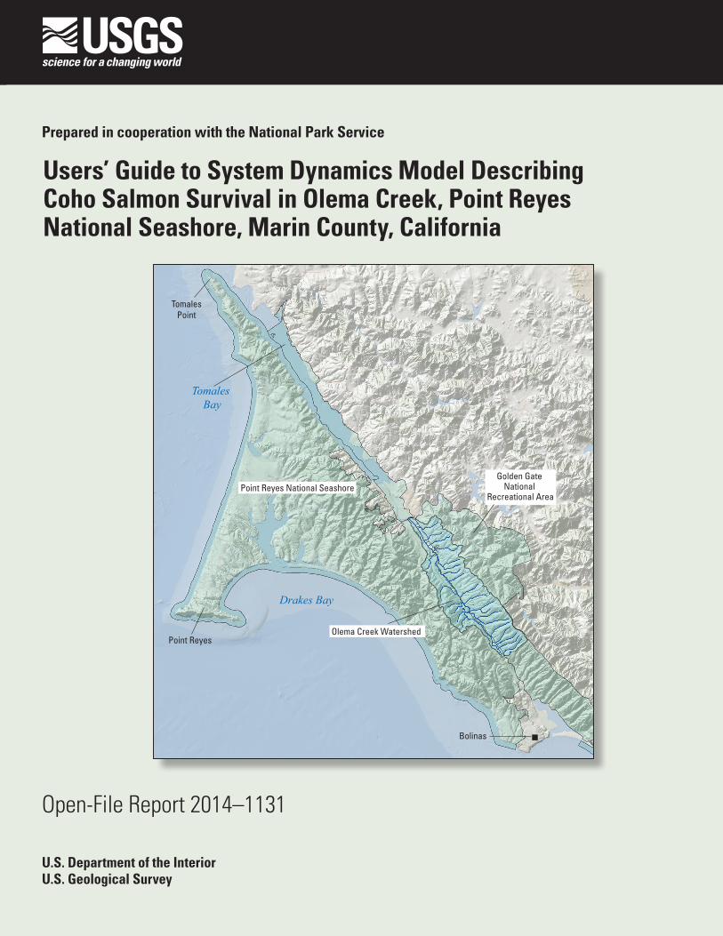
Users’ Guide to System Dynamics Model Describing Coho Salmon Survival in Olema Creek, Point Reyes National Seashore, Marin County, California

U.S. Department of the InteriorU.S. Geological Survey

Open-File Report 2014–1131

Users’ Guide to System Dynamics Model Describing Coho Salmon Survival in Olema Creek, Point Reyes National Seashore, Marin County, California

By Andrea Woodward, Alicia Torregrosa, Mary Ann Madej, Michael Reichmuth, and Darren Fong

Prepared in cooperation with the National Park Service

Open-File Report 2014–1131

U.S. Department of the Interior U.S. Geological Survey

U.S. Department of the Interior SALLY JEWELL, Secretary

U.S. Geological Survey Suzette M. Kimball, Acting Director

U.S. Geological Survey, Reston, Virginia: 2014

For more information on the USGS—the Federal source for science about the Earth, its natural and living resources, natural hazards, and the environment—visit http://www.usgs.gov or call 1–888–ASK–USGS

For an overview of USGS information products, including maps, imagery, and publications, visit http://www.usgs.gov/pubprod

To order this and other USGS information products, visit http://store.usgs.gov

Suggested citation: Woodward, Andrea, Torregrosa, Alicia, Madej, Mary Ann, Reichmuth, Michael, and Fong, Darren, 2014, Users’ guide to system dynamics model describing Coho salmon survival in Olema Creek, Point Reyes National Seashore, Marin County, California: U.S. Geological Survey Open-File Report 2014-1131, 58 p., http://dx.doi.org/10.3133/ofr20141131. ISSN 2331-1258 (online)

Any use of trade, firm, or product names is for descriptive purposes only and does not imply endorsement by the U.S. Government.

Although this information product, for the most part, is in the public domain, it also may contain copyrighted materials as noted in the text. Permission to reproduce copyrighted items must be secured from the copyright owner.

iii

Contents Background ................................................................................................................................................................... 1 Model Overview ............................................................................................................................................................. 3

Coho Life Cycle .......................................................................................................................................................... 3 Model Software and Requirements ............................................................................................................................ 6 Data Sources ............................................................................................................................................................. 6 Model Summary ......................................................................................................................................................... 7

Parameters and Relationships in Model .......................................................................................................................11 Eggs to Juveniles in Early Summer (Model Weeks 1-25) .........................................................................................11

Introduction (Spring: December through May) .......................................................................................................11 Model Stocks (Spring: December through May) ....................................................................................................13 Model Flows (Spring: December through May) .....................................................................................................14 Model Converters (Spring: December through May) .............................................................................................15

Juveniles from Early Summer to Late Summer (Model Weeks 26-45) ......................................................................18 Introduction (Summer: June to mid-October) ........................................................................................................18 Model Stocks (Summer: June to mid-October) ......................................................................................................19 Model Flows (Summer: June to mid-October) .......................................................................................................20 Model Converters (Summer: June through mid-October) ......................................................................................21

Juveniles in Late Summer to Smolts (Model Weeks 46–75) .....................................................................................30 Introduction (Winter-Spring2: mid-October through April)......................................................................................30 Model Stocks (Winter-Spring2: mid-October through April) ...................................................................................32 Model Flows (Winter-Spring2: mid-October through April) ....................................................................................32 Model Converters (Winter-Spring2: mid-October through April) ............................................................................33

Results—Comparison of Model Output with Data.........................................................................................................37 Potential Uses of Model ................................................................................................................................................39 Model Limitations ..........................................................................................................................................................40 Acknowledgments ........................................................................................................................................................40 References Cited ..........................................................................................................................................................41 Appendix A. Input Spreadsheet Format ........................................................................................................................45 Appendix B. Acquiring and Running Model ..................................................................................................................47 Appendix C. Model Equations ......................................................................................................................................57

Figures Figure 1. Diagram showing coho salmon lifecycle ........................................................................................................ 3 Figure 2. Schematic showing system dynamics model indicating stocks, primary flows, and main factors affecting flows ................................................................................................................................................................ 7 Figure 3. Diagram showing section of model describing survival of fish from the egg stage to juveniles in early summer (JuvenilesES) from December through May as it appears in Stella®. ........................................................... 12 Figure 4. Graph showing regression of additional mortality greater than baseline value against number of fry stress-flow events for spawning years 2002–03 through 2006–07. ........................................................................ 17 Figure 5. Diagram showing section of model describing survival of juveniles over summer from June through mid-October as it appears in Stella® ............................................................................................................... 18 Figure 6. Graph showing regression of juveniles late in summer against juveniles early in summer for years when juvenile surveys occurred at the end of summer ..................................................................................... 21

iv

Figure 7. Graph showing relationship between flow and dissolved oxygen concentration as measured on Olema Creek at John West Fork above the Highway 1 culvert, an area observed by authors to have good coho rearing habitat ..................................................................................................................................................... 23 Figure 8. Graph showing regression of weekly average water temperature during summer against weekly average air temperature for June through mid-October, 2003–10 ................................................................... 24 Figure 9. Graph showing fraction of maximum fish capacity realized as a function of the number of summer weekly low flows below 0.2 cubic feet per second (ft3/s) each year. .............................................................. 26 Figure 10. Graph showing comparisons among observed smolt counts and predicted smolts using Ricker and Beverton-Holt equations (Guy and Brown, 2007). ....................................................................................................... 27 Figure 11. Graph showing evidence of density dependence of fish ............................................................................ 29 Figure 12. Diagram showing section of model describing survival of juveniles over second winter and spring until they become smolts from mid-October through April as it appears in Stella® ............................................ 31 Figure 13. Graph showing effect of winter habitat on winter survival of salmon .......................................................... 36 Figure 14. Graph showing comparison of modeled juvenile numbers with actual juvenile data .................................. 37 Figure 15. Graph showing comparison of modeled smolt numbers with actual data, 2002–2010 ............................... 38

Tables Table 1. Life history stage determined from National Park Service (2010) monitoring data .......................................... 4 Table 2. Model elements, definitions, sources, and confidence .................................................................................... 9 Table 3. Mortality due to scouring flow events ............................................................................................................ 15

Conversion Factors Inch/Pound to SI

Multiply By To obtain

Flow rate foot per second 30.48 centimeter per second (cm/s)

foot per second 0.3048 meter per second (m/s)

cubic foot per second (ft3/s) 0.02832 cubic meter per second (m3/s) SI to Inch/Pound

Multiply By To obtain

Length

centimeter (cm) 0.3937 inch (in.)

meter (m) 3.281 foot (ft)

kilometer (km) 0.6214 mile (mi)

Area

square meter (m2) 0.0002471 acre

square kilometer (km2) 247.1 acre

square kilometer (km2) 0.3861 square mile (mi2) Temperature in degrees Celsius (°C) may be converted to degrees Fahrenheit (°F) as follows:

ºF=(1.8×°C)+32.

1

Users’ Guide to System Dynamics Model Describing Coho Salmon Survival in Olema Creek, Point Reyes National Seashore, Marin County, California

By Andrea Woodward1, Alicia Torregrosa1, Mary Ann Madej1, Michael Reichmuth2, and Darren Fong2

Background The system dynamics model described in this report is the result of a collaboration

between U.S. Geological Survey (USGS) scientists and National Park Service (NPS) San Francisco Bay Area Network (SFAN) staff, whose goal was to develop a methodology to integrate inventory and monitoring data to better understand ecosystem dynamics and trends using salmon in Olema Creek, Marin County, California, as an example case. The SFAN began monitoring multiple life stages of coho salmon (Oncorhynchus kisutch) in Olema Creek during 2003 (Carlisle and others, 2013), building on previous monitoring of spawning fish and redds. They initiated water-quality and habitat monitoring, and had access to flow and weather data from other sources.

This system dynamics model of the freshwater portion of the coho salmon life cycle in Olema Creek integrated 8 years of existing monitoring data, literature values, and expert opinion to investigate potential factors limiting survival and production, identify data gaps, and improve monitoring and restoration prescriptions. A system dynamics model is particularly effective when (1) data are insufficient in time series length and/or measured parameters for a statistical or mechanistic model, and (2) the model must be easily accessible by users who are not modelers. These characteristics helped us meet the following overarching goals for this model:

• Summarize and synthesize NPS monitoring data with data and information from other sources to describe factors and processes affecting freshwater survival of coho salmon in Olema Creek.

• Provide a model that can be easily manipulated to experiment with alternative values of model parameters and novel scenarios of environmental drivers.

1 U.S. Geological Survey. 2 National Park Service.

2

Although the model describes the ecological dynamics of Olema Creek, these dynamics are structurally similar to numerous other coastal streams along the California coast that also contain anadromous fish populations. The model developed for Olema can be used, at least as a starting point, for other watersheds. This report describes each of the model elements with sufficient detail to guide the primary target audience, the NPS resource specialist, to run the model, interpret the results, change the input data to explore hypotheses, and ultimately modify and improve the model. Running the model and interpreting the results does not require modeling expertise on the part of the user. Additional companion publications will highlight other aspects of the model, such as its development, the rationale behind the methodological approach, scenario testing, and discussions of its use.

System dynamics models consist of three basic elements: stocks, flows, and converters. Stocks are measurable quantities that can change over time, such as animal populations. Flows are any processes or conditions that change the quantity in a stock over time (Ford, 1999), are expressed in the model as a rate of change, and are diagrammed as arrows to or from stocks. Converters are processes or conditions that change the rate of flows. A converter is connected to a flow with an arrow indicating that it alters the rate of change. Anything that influences the rate of change (such as different environmental conditions, other external factors, or feedbacks from other stocks or flows) is modeled as a converter. For example, the number of fish in a population is appropriately modeled as a stock. Mortality is modeled as a flow because it is a rate of change over time used to determine the number of fish in the population. The density-dependent effect on mortality is modeled as a converter because it influences the rate of morality. Together, the flow and converter change the number, or stock, of juvenile coho. The instructions embedded in the stocks, flows, converters, and the sequence in which they are linked are processed by the simulation software with each completed sequence composing a model run. At each modeled time step within the model run, the stock counts will go up, down, or stay the same based on the modeled flows and the influence of converters on those flows.

The model includes a user-friendly interface to change model parameters, which allows park staff and others to conduct sensitivity analyses, incorporate future knowledge, and implement scenarios for various future conditions. The model structure incorporates place holders for relationships that we hypothesize are significant but data are currently lacking. Future climate scenarios project stream temperatures higher than any that have ever been recorded at Olema Creek. Exploring climate change impacts on coho survival is a high priority for park staff, therefore the model provides the user with the option to experiment with hypothesized effects and to incorporate effects based on future observations.

3

Model Overview Coho Life Cycle

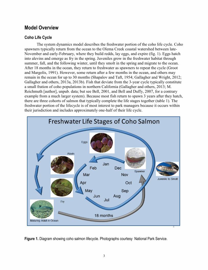
The system dynamics model describes the freshwater portion of the coho life cycle. Coho spawners typically return from the ocean to the Olema Creek coastal watershed between late-November and early-February, where they build redds, lay eggs, and expire (fig. 1). Eggs hatch into alevins and emerge as fry in the spring. Juveniles grow in the freshwater habitat through summer, fall, and the following winter, until they smolt in the spring and migrate to the ocean. After 18 months in the ocean, they return to freshwater as spawners to repeat the cycle (Groot and Margolis, 1991). However, some return after a few months in the ocean, and others may remain in the ocean for up to 30 months (Shapalov and Taft, 1954; Gallagher and Wright, 2012; Gallagher and others, 2013a, 2013b). Fish that deviate from the 3-year cycle typically constitute a small fration of coho populations in northern California (Gallagher and others, 2013; M. Reichmuth [author], unpub. data; but see Bell, 2001, and Bell and Duffy, 2007, for a contrary example from a much larger system). Because most fish return to spawn 3 years after they hatch, there are three cohorts of salmon that typically complete the life stages together (table 1). The freshwater portion of the lifecycle is of most interest to park managers because it occurs within their jurisdiction and includes approximately one-half of their life cycle.

Figure 1. Diagram showing coho salmon lifecycle. Photographs courtesy National Park Service.

4

Table 1. Life history stage determined from National Park Service (2010) monitoring data. [Shading color indicates cohorts]

Spaw

ning

Yea

r

Redd

s (wa

ters

hed

redd

tota

l)g

Aver

age f

emale

fork

leng

th (c

m)b

Estim

ated

num

ber o

f egg

sc

Basin

wide

juve

nile

estim

ate

Estim

ated

surv

ival r

ate e

gg to

ju

veni

le (%

)

Mont

h of

juve

nile

surv

ey

Wat

ersh

ed sm

olt p

rodu

ctio

n es

timat

e

Mean

smol

t len

gth

(mm

)

Mean

smol

t weig

ht (g

)

Estim

ated

surv

ival r

ate j

uven

ile to

sm

olt (

%)

Estim

ated

surv

ival r

ate e

gg to

sm

olt (

%)

Estim

ated

surv

ival r

ate s

mol

t to

adul

t (%

)e

Estim

ated

surv

ival r

ate j

uven

ile to

ad

ult (

%)e

2002-2003 22a 64.0 51,876h 11,926±3,244 23.0 6 831±167d 114 15.1 7.0h 1.6 2.4 0.2 2003-2004 107 66.3 279,904 25,857±1499 9.2 6 362±145m 116 16.0 1.4m 0.1m 52.5n,m 0.7 2003-2004 corrected 1,629 6.3 0.6 8.4 2004-2005 136 65.7 346,382 29,887±9,974 8.6 6 3,793±784 99l 10.3 12.7 1.1 1.4 0.2 2005-2006 10a 58.7 18,288p 1,793±869i 9.8q 6 1,485±206 116 14.7 82.8n 8.1 0 0 2005-2006 corrected 2,200 67.5 2006-2007 95 65.3 237,652 32,298±4,018 13.6 7 2,885±336 111 12.4 8.9 1.2 1.0 0.1 2007-2008 26 64.0 61,308 3,328±696o 5.4o 10 4,088±1,041 113 12.9 122.3o 6.7 1.0 1.3 2007-2008 corrected 5,088 8.3 80.0 2008-2009 0k 64.0 0 0 0 8-10 10f 136 24.1 N/A N/A SY2011-12 SY2011-12 2009-2010 14 57.2 23,726 1,736±659 7.3 8-9 1435±463 82.7 6.0 SY2012-13 SY1012-13 aDue to poor observer efficiency, the peak live plus cumulative dead index (PLD) (Beidler and Nickelson, 1980; Johnston and others, 1987) was used to estimate the Olema Creek mainstem redd count based on two spawners per redd. b Average female fork length based on female carcass lengths on Olema Creek for spawning years 2003–04 through 2007–2008. c Estimated number of eggs using Shapovalov and Taft (1954) formula based on average female fork length. d Tagging procedures for smolt counts and derivation of final smolt count were not well documented; therefore, this estimate cannot be verified or recalculated (M. Reichmuth, author). However, smolt production was estimated to be low this year in Lagunitas Creek (Stillwater Sciences, 2008). e Estimated smolt to adult calculated by dividing number of adult spawners (estimated based on two times the total watershed redd count) divided by the estimated number of outmigrating smolts for previous cohort. f Raw count. gIncludes John West Fork red count. hNumber is suspect (M. Reichmuth, author).

5

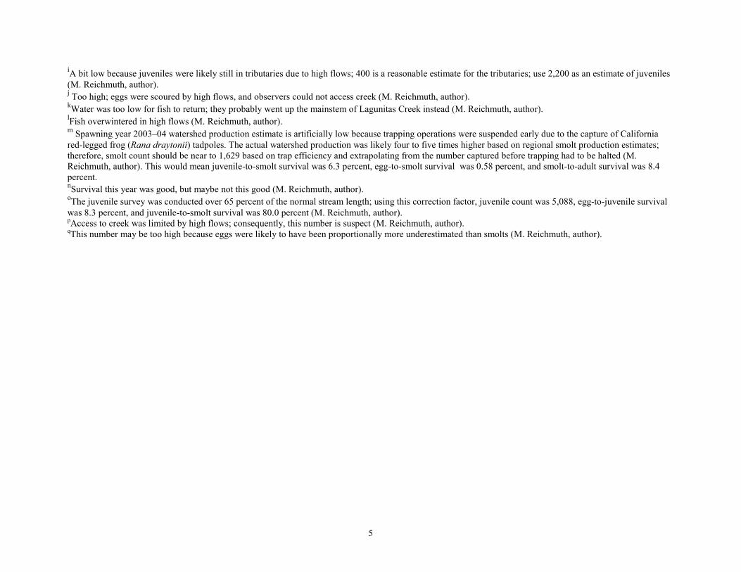
iA bit low because juveniles were likely still in tributaries due to high flows; 400 is a reasonable estimate for the tributaries; use 2,200 as an estimate of juveniles (M. Reichmuth, author). j Too high; eggs were scoured by high flows, and observers could not access creek (M. Reichmuth, author). kWater was too low for fish to return; they probably went up the mainstem of Lagunitas Creek instead (M. Reichmuth, author). lFish overwintered in high flows (M. Reichmuth, author). m Spawning year 2003–04 watershed production estimate is artificially low because trapping operations were suspended early due to the capture of California red-legged frog (Rana draytonii) tadpoles. The actual watershed production was likely four to five times higher based on regional smolt production estimates; therefore, smolt count should be near to 1,629 based on trap efficiency and extrapolating from the number captured before trapping had to be halted (M. Reichmuth, author). This would mean juvenile-to-smolt survival was 6.3 percent, egg-to-smolt survival was 0.58 percent, and smolt-to-adult survival was 8.4 percent. nSurvival this year was good, but maybe not this good (M. Reichmuth, author). oThe juvenile survey was conducted over 65 percent of the normal stream length; using this correction factor, juvenile count was 5,088, egg-to-juvenile survival was 8.3 percent, and juvenile-to-smolt survival was 80.0 percent (M. Reichmuth, author). pAccess to creek was limited by high flows; consequently, this number is suspect (M. Reichmuth, author). qThis number may be too high because eggs were likely to have been proportionally more underestimated than smolts (M. Reichmuth, author).

6

Model Software and Requirements The freshwater life cycle of coho salmon in Olema Creek was modeled using the Stella

10.0.3® system dynamics simulation software (http://www.iseesystems.com). Several other commercial and open-source software packages are available, including MapleSim®, PowerSim®, Simulink®, Vensim®, and many others. The following description of our use of Stella® software and all references to non-USGS products and services are provided for information only and do not constitute endorsement or warranty, express or implied, by the USGS, U.S. Department of the Interior, or any other body of the U.S. Federal Government.

Basic components required to build the model include: • Population estimates for key life stages or stocks. • Information on habitat and physical drivers contributing to survival or mortality. • Sources of quantitative relationships among mortality and population stressors derived

from literature review and expert opinion. • Local experts to provide and adjust parameters and mortality levels when locally

collected data are not available. Olema Creek is the largest undammed watershed in coastal Marin County, California,

flowing for 15.9 km northwest through the Olema Valley, the landward expression of the San Andreas Fault Zone. Currently protected from development, the 37.6 km2 watershed is primarily contained within the boundaries of Point Reyes National Seashore and Golden Gate National Park North District (Carlisle and others, 2013). Impacts to the watershed due to historical land use include logging, channelization, and agricultural operations; presently, the primary human impacts include on-going agricultural operations and management of Highway 1. Geologic activity along the San Andreas Fault and local weather patterns also affect the creek.

Data Sources Every year, the NPS conducts a census of coho redds in winter, samples the size of coho

females, estimates eggs from winter redd surveys and female size, counts juveniles using snorkel surveys at the beginning and end of summer, and counts smolts with smolt traps in spring. The estimates are published in NPS annual reports (http://www.sfnps.org/coho/reports/); however, these estimates are challenging to use because they cannot be cited as published data (table 1). The record begins in 2002, but there was a lack of confidence in some of the earlier estimates. More recent records with unexpectedly high or low estimates are attributable to variations in survey methods and specific areas surveyed. Specific variations include changes to the protocol over years, loss of access to normally sampled areas due to weather and flow conditions, equipment failure due to weather, and inability of spawners to return due to low flow. After careful assessment of each number in the table, authors involved in data collection were able to make corrections to account for adverse sampling events. Data labeled as ‘corrected’ in table 1 were used in the model.

In addition to fish population data, NPS monitors beginning and end of fish spawning period, habitat descriptors, and water-quality parameters, of which we used dissolved oxygen (DO) data. NPS operates the USGS streamgage on Olema Creek at the Bear Valley Road bridge (USGS 11460610) and has unpublished data used to estimate flow volume from flow rate. NPS also operates the Olema Valley Remote Automated Weather Stations (RAWS) station (ID 3287D6FE) located approximately 520 m from the Olema streamgage, which was the source of air temperature data.

7

Other data sources include include the Lagunitas Creek limiting factors study (Stillwater Sciences, 2008) for fish population data. Flow data from a streamgage on San Geronimo Creek operated by Balance Hydrologics for Marin County were used to estimate Olema flow during periods of instrument failure at the Olema streamgage.

Model Summary The model consists of four stocks representing four stages in the coho life cycle: eggs,

juveniles in early summer, juveniles in late summer, and smolts (fig. 2). These stages were selected to model because some data exist for each during the 8-year period of record (table 1). Early in the record, juvenile data were collected early in the summer but later, they were collected in August and September. This inconsistency enabled us to evaluate summer mortality effects. Summer mortality is important because summer is a potentially stressful time for fish in Olema Creek if flows are low (dry years), a condition that is anticipated to become increasingly common due to climate change (Madej, 2012).

Figure 2. Schematic showing system dynamics model indicating stocks, primary flows, and main factors affecting flows.

8

Fish move from one stock to the next through the flow of ‘survival,’ which is calculated as the number of fish remaining after losses due to mortality have been subtracted from the stock (fig. 2). Once fish have left the system or died, they are represented in the model as having disappeared into a ‘cloud’ icon and are no longer accounted for. Factors affecting each transition include several characteristics of streamflow, water temperature, and habitat availability, plus a baseline mortality to reflect effects not specifically modeled. ‘Fry-stress streamflows’ are flow levels that threaten to wash the fish downstream unless they put their energy into swimming rather than feeding.

The model simulates an individual year and runs on a weekly time step to reflect the resolution of fish surveys. Time intervals for each section of the model were provided by NPS staff. Inputs to the model include the initial number of eggs for each year, a habitat index, and weekly streamflow and air temperature values. These inputs are imported into the model from an Excel® spreadsheet according to the format in appendix A. Because the marine environment is outside of NPS jurisdiction and oceanic factors affecting salmon are largely unmonitored or unknown, the model does not include returning adults.

An interactive interface provides slider bars to adjust select mortality factors. This is intended to give the user the option of adjusting the values at various fish life cycle phases to simulate historical or novel environmental conditions and to conduct sensitivity analyses. Instructions for acquiring and running the model, making changes, and conducting several simple analyses are provided in appendix B.

The following section describes in detail the parameters and relationships driving each section of the model and their derivation from NPS monitoring and other data sources. Documentation of parameter formulation also is in the model itself. An abbreviated reference guide to model elements is provided in table 2. Model elements, as named in the model, are included in the text using distinct font, and titles of stocks are capitalized. For example, JuvenilesES is the model element describing the number of juveniles in early summer. All model equations are given in appendix C.

9

Table 2. Model elements, definitions, sources, and confidence. [Type: C, converter; F, flow; S, stock; Conf., confidence in data or relationship; Expert, expert opinion; Med, medium. Source: NPS, data from National Park Service; Hypoth, hypothesized relationship; Lit, values from literature; Other, data from sources other than NPS] [Note: Names of stocks are capitalized throughout the document.]

Model element Type Definition Source Conf.

annual summer juv max C Fraction of potential carrying capacity realized in a particular year NPS Low base mortality spring C Mortality not attributable to factors explicitly included in model, December

through May NPS Med

base mortality summer C Mortality not attributable to factors explicitly included in model, June to mid-October

NPS Med

base mortality wint spr2 C Mortality not attributable to factors not explicitly included in model, mid-October through April

NPS Med

beg of spawn C Week when spawning begins NPS High Critical min summer flow count

S Number of weeks with critically low flows from June through mid-October Other High

density threshold wint spr2 C Carrying capacity of Olema Creek for juvenile coho, mid-October through April NPS Low DO threshold C Dissolved oxygen (DO) level below which fish are harmed Lit Med Eggs S Estimate of annual egg count NPS High end of spawn C Week when spawning ends NPS High Fry event count S Number of events when high streamflow forces fish to swim against the current

rather than feed Other High

fry mort event C Criteria determining whether amount and timing of weekly flow constitute an event that causes stress to fry

Expert Med

fry flow threshold C Weekly maximum of daily flow values that constitutes a fry stress event Expert Med habitat index C Index describing habitat quality, mid-October through April NPS Low habitat threshold C Threshold of habitat index below which fish mortality increases Hypoth Low initial eggs C Mechanism for inputting annual egg estimate NPS High JuvenilesES S Number of juvenile fish in early summer NPS High JuvenilesLS S Number of juvenile fish in mid-October NPS High juvenile summer max C Maximum summer carrying capacity for fish under ideal conditions NPS Med mort density wint spr2 C Density-dependent mortality of juvenile fish, mid-October through April NPS Low mort DO C Apply fish mortality due to low dissolved oxygen (DO) if weekly minimum flow

indicates DO below threshold Lit Low

mort DO factor C Mortality attributed to fish due to flows below the DO threshold NPS Low mort fry events C Mortality attributed to fry stress-flow events NPS Med mort habitat C Apply habitat-related mortality when habitat index is below the threshold Hypoth Low

10

Model element Type Definition Source Conf. mort habitat factor C Increase in fish mortality due to poor habitat quality Hypoth Low mort hfe wint spr2 C Mortality due to high-flow events, mid-October through April Hypoth Low mort pred C Apply fish mortality due to predation if streamflow is below predation threshold Hypoth Low mort pred factor C Fish mortality due to weekly minimum flows below the predation threshold Hypoth Low mort scour events C Rate of mortality due to scouring flow events NPS Med mort stream temp C Apply fish mortality due to stream temperature exceeding temperature threshold Hypoth Low pred threshold C Weekly minimum of daily streamflow below which mortality due to predation

increases Hypoth Low

Scour event count S Number of scouring flow events Other High scour event C Criteria determining whether amount and timing of flow constitute a scouring flow

event Expert Med

scour threshold C Streamflow value above which redds are likely to be scoured from streambed Expert Med Smolts S Number of smolts at end of April NPS High spring high flow C Weekly maximum of average daily stream flow, December through May Other High spring mortality F Mortality of fish from eggs to juveniles, December through May NPS Med spring survival F Survival of fish from eggs to juveniles, December through May NPS Med stream temp mort factor C Fish mortality due to weekly stream temperature exceeding the threshold Hypoth Low stream temp threshold C Stream temperature above which fish show increased mortality Lit Med summer average air temp C Weekly average of daily average air temperature Other High summer critical flow C Model flow that determines whether the weekly minimum of daily streamflow

value constitutes a critical flow NPS Med

summer critical flow threshold Streamflow threshold below which juvenile mortality increases NPS Low summer min flow C Weekly minimum of average daily streamflow, June to mid-October Other High summer mortality F Mortality of juvenile fish, June to mid-October NPS Low summer survival F Survival of juvenile fish, June to mid-October NPS Low wint spr2 hfe F Adds to count if weekly high flow constitutes a high-flow event Other High winter spr2 hfe count S Number of high-flow events that increase fish mortality, mid-October through

April Other High

wint spr2 hfe mort factor C Increased fish mortality due to high-flow event, mid-October through April Hypoth Low wint spr2 high flow C Weekly maximum high streamflow, mid-October through April Other High wint spr2 high flow threshold C High streamflow threshold at which fish mortality increases Expert Med wint spr2 mortality F Mortality of fish from juveniles to smolts, mid-October through April NPS Med wint spr2 survival F Survival of fish from juveniles to smolts, mid-October through April NPS Med

11

Parameters and Relationships in Model Eggs to Juveniles in Early Summer (Model Weeks 1-25)

Introduction (Spring: December through May) The first section of the model simulates factors affecting survival of fish from the egg

stage to juveniles in early summer (JuvenilesES). The schematic representation as a Stella® diagram is shown in figure 3. Model terms, their definitions, sources and confidence and relationship to one another are given in table 2. This section of the model includes the 25 weeks from December through May (model weeks 1–25) when eggs are expected to be deposited and have adequate time to mature to the juvenile stage but before they are subject to summer low-flow conditions. The primary stocks are labeled Eggs (number of eggs deposited by adult coho females) and JuvenilesES (population of remaining young-of-year juvenile coho). Model flows are labeled spring mortality, which depletes eggs, and spring survival, which is determined as the remaining eggs at the end of the time period. Deceased eggs and fish flow into a ‘cloud’ where they are no longer tracked in the model.

Factors affecting mortality are represented as converters in the model (fig. 3). Factors include baseline mortality due to drivers not explicitly modeled, scouring flow events that destroy redds, and flows high enough to force fish to swim rather than feed (fry events). Evidence of non-density-dependent mortality of eggs and fry in spring is described in a limiting factors analysis of the Lagunitas Creek watershed (Stillwater Sciences, 2008) and in coho monitoring data collected by the Marin County Water District (Ettlinger and others, 2006). Although the limiting factor analysis found no evidence that scouring or entombment of eggs and alevins are occurring, it did find indirect evidence that fry displacement could be having an effect (Stillwater Sciences, 2008). Nevertheless, the limiting factor analysis did consider that flows at twice bankfull could be considered scouring flows. We modeled both scour and fry events as flow exceeding appropriate thresholds (see details and rationale in “Model Converters” section below). Effects are modeled as functions of the number of these events.

12

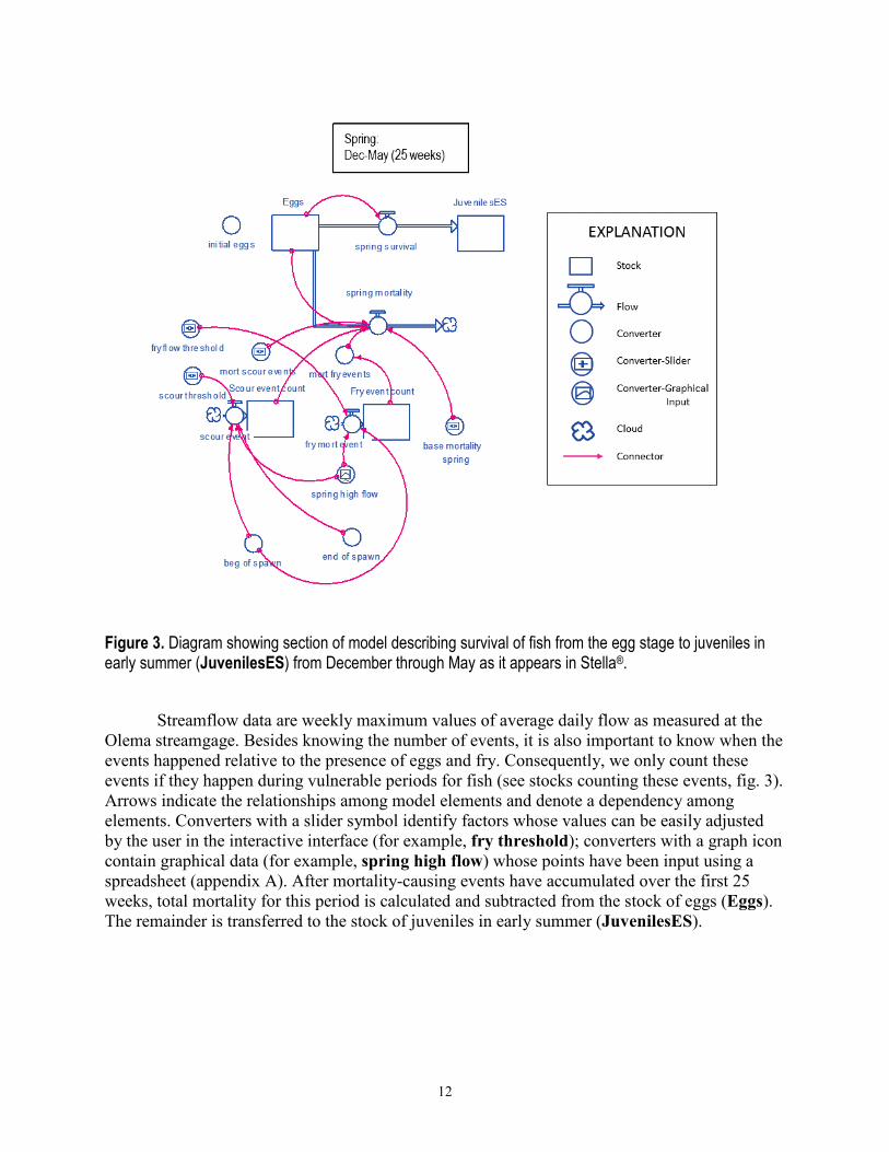
Figure 3. Diagram showing section of model describing survival of fish from the egg stage to juveniles in early summer (JuvenilesES) from December through May as it appears in Stella®.

Streamflow data are weekly maximum values of average daily flow as measured at the

Olema streamgage. Besides knowing the number of events, it is also important to know when the events happened relative to the presence of eggs and fry. Consequently, we only count these events if they happen during vulnerable periods for fish (see stocks counting these events, fig. 3). Arrows indicate the relationships among model elements and denote a dependency among elements. Converters with a slider symbol identify factors whose values can be easily adjusted by the user in the interactive interface (for example, fry threshold); converters with a graph icon contain graphical data (for example, spring high flow) whose points have been input using a spreadsheet (appendix A). After mortality-causing events have accumulated over the first 25 weeks, total mortality for this period is calculated and subtracted from the stock of eggs (Eggs). The remainder is transferred to the stock of juveniles in early summer (JuvenilesES).

13

Model Stocks (Spring: December through May) [Stocks are measurable quantities that can change over time.] Eggs (the annual egg estimate for each spawning year): Annual egg counts are estimated based

on redd surveys and average female fork length from recovered carcasses using the equation of Shapovalov and Taft (1954) for estimating the number of eggs per female. Number of eggs is input into the model from a spreadsheet (appendix A).

Juveniles ES (number of juvenile fish in early summer): Juveniles in early summer represent those fish surviving from egg through the alevin and fry stages to become juveniles. Juveniles were counted in early summer during only 5 years (table 1), but these data are sufficient to provide some basis for separating spring effects from summer effects. This is one example of a relationship that can be validated as future data are collected and incorporated into the model.

Scour event count (high-flow conditions that destroy redds): Scour events are rare (Montgomery and others, 1996), but devastating, and may increase in frequency due to climate change (Dettinger, 2011). The value is set using the scour threshold converter (see section “Scour Event Count”).

Fry event count (periods when high flow forces fry to maintain their position in the creek channel rather than actively foraging for food): Small fish are especially vulnerable to these conditions (Quinn, 2005).

14

Model Flows (Spring: December through May) [Flows are rates of change in stocks per unit of time.] spring mortality (mortality of fish occurring from egg to juvenile during December through

May): Spring mortality is calculated at week 26 and is determined to be 97 percent (mort scour events) if there has been a scouring flow event. Otherwise, mortality is determined as baseline mortality plus mortality due to fry stress flow events. The number of eggs lost is the initial number of eggs multiplied by mortality. The model equation reads ‘if time = 26 then eggs * (if scour_events > 0 then mort_scour_events else (base_mortality_fraction + mort_fry_events)) else 0.’

spring survival (survival of fish from egg to juvenile during December through May): Spring survival is simply the initial egg count minus the number of eggs lost due to mortality. This number is transferred to the stock of juveniles in early summer (JuvenilesES).

scour event (criteria determining whether the amount and timing of weekly flows constitute a scouring event that will affect eggs and should be added to the scour event stock): Scour events are counted if they occur after the beginning of spawning and before 11 weeks after spawning ends. After this period, it is expected that most eggs will have hatched and escaped the spawning gravel as fry (Shapovalov and Taft, 1954; Groot and Margolis, 1991). Although these fish are still vulnerable to scouring floods, they have greater mobility to find shelter at stream edges. By this time of year, they are more susceptible to fry stress flow events than scour events under the current hydrograph. However, the hydrograph may change due to climate change, and consequently data may become available to redefine this relationship. The model equation reads ‘if (spring_high_flow > scour_threshold) and time > end_of_spawn and time < (beg_of_spawn +11) then 1 else 0.’

fry mort event (criteria determining whether amount and timing of weekly flow constitutes an event that causes stress to fry and should be added to the fry stress event stock): Fry stress flow events, which increase mortality, are counted after the beginning of spawning plus 7 weeks and before week 23 (week of May 1) because seven weeks is the minimum time for fry to emerge from redds (Shapovalov and Berrian, 1940; Shapovalov and Taft, 1954). Also, experts felt that these types of events are very unlikely to occur after May 1, and it was safe to simplify the relationship by not tying the end of the counting period to spawning observations. The model equation reads ‘if (beg_of_spawn ) < time and time < 23 and spring_high_flow > fry_threshold) then 1 else 0.’

15

Model Converters (Spring: December through May) In this section, converters are factors that affect rates of the model flow spring mortality, either

directly or by affecting other converters or stocks. Converters that affect other converters or stocks are indented on the page under the affected stock or converter.

initial eggs (annual estimate of eggs based on monitoring data): A converter containing the annual egg

count is simply the mechanism in Stella® for introducing the annual value entered from the input spreadsheet (appendix A) into the model. The lack of an arrow connecting this converter to anything means that it is only used once to initiate the model.

base mortality spring (mortality from egg to juvenile during spring that is not attributable to factors explicitly included in the model): Baseline mortality spring is estimated to be 77 percent based on survival for spawning year 2002–03, which was the highest value for years when juveniles were counted at the beginning of the summer (table 1).

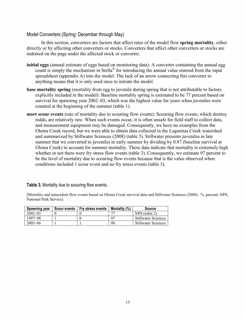
mort scour events (rate of mortality due to scouring flow events): Scouring flow events, which destroy redds, are relatively rare. When such events occur, it is often unsafe for field staff to collect data, and measurement equipment may be damaged. Consequently, we have no examples from the Olema Creek record, but we were able to obtain data collected in the Lagunitas Creek watershed and summarized by Stillwater Sciences (2008) (table 3). Stillwater presents juveniles in late summer that we converted to juveniles in early summer by dividing by 0.87 (baseline survival at Olema Creek) to account for summer mortality. These data indicate that mortality is extremely high whether or not there were fry stress flow events (table 3). Consequently, we estimate 97 percent to be the level of mortality due to scouring flow events because that is the value observed when conditions included 1 scour event and no fry stress events (table 3).

Table 3. Mortality due to scouring flow events. [Mortality and antecedent flow events based on Olema Creek survival data and Stillwater Sciences (2008). %, percent; NPS, National Park Service] Spawning year Scour events Fry stress events Mortality (%) Source 2002–03 0 0 77 NPS (table 2) 1997–98 1 0 97 Stillwater Sciences 2005–06 1 1 98 Stillwater Sciences

16

Scour event count (stock that counts scour events, see section, “Stocks”)

spring high flow (weekly maximum of average daily streamflow): These values are measured at the Olema Creek streamgage. These values are input into the model using a spreadsheet (appendix A).

beg of spawn (week when spawning begins): Beginning of spawn is the week when redds were first counted from the first week of December. Count data are input into the model using a spreadsheet (appendix A).

end of spawn (last week of spawning): End of spawn is the week counted from the first week of December when the last redds were observed to be constructed. Count data are input into the model using a spreadsheet (appendix A).

scour threshold (flow value above which redds are likely to be scoured from the streambed): Although mobilization of coarse streambed material has been observed to begin at bankfull discharge (Andrews, 1983), the Lagunitas Limiting Factors report (Stillwater Sciences, 2008) concluded that a bankfull flow event (end of 2005) did not cause redd-destroying scour on Lagunitas Creek. However, Stillwater Sciences (2008) does consider twice bankfull flow to be an appropriate threshold for scour. The event at the end of 2005 was likely a twice bankfull event on Olema Creek, and was the highest flow observed during the period with salmon data. The streamgage at Olema Creek failed during this event, but flow at nearby San Geronimo Creek was 1,090 ft3/s. Olema and San Geronimo Creeks do not have a completely consistent correlation, but for flows where at least one of the sites had flow greater than 500 ft3/s—San Geronimo Creek averaged 498 ft3/s, and Olema Creek averaged 563 ft3/s—so for high flows, we can approximate Olema Creek flow with data from San Geronimo Creek. Flow of 1,090 ft3/s is approximately twice bankfull on Olema Creek, where 500 ft3/s is considered bankfull flow (based on Dunne and Leopold, 1978). Stillwater Sciences (2008) observed one redd to be scoured on Olema Creek during this event and NPS staff consider this event to constitute scouring flow. Consequently, we use 1,090 ft3/s as the threshold for redd scour.

17

mort fry events (mortality attributed to fry stress-flow events): Mortality due to fry stress-flow events was calculated as 4.46 × ln(fry events) + 10.93 based on the regression of additional mortality above baseline against number of fry events for spawning years 2002–03 through 2006–07 (fig. 4). These are years when juveniles were counted at the beginning of summer. Our results contradict those of Gallagher and others (2012), who found no relationship between streamflow and egg to juvenile survival in another small northern California stream.

Fry event count (stock that counts the number of fry events): See section, “Model Stocks”. spring high flow (weekly maximum of average daily streamflow): These values are

measured at the Olema Creek streamgage. beg of spawn (week when spawning begins). fry threshold (weekly maximum of daily flow values that constitutes a fry stress event):

Fry are vulnerable to displacement downstream by streamflows that exceed their swimming strength (Ottawya and Clark, 1981; Harvey, 1987; Heggenes and Traaen, 1988; Quinn, 2005). Fry are especially vulnerable in streams having few refuges due to reduced channel complexity. NPS authors also thought that fry may be stressed by flows high enough to require activity to resist, thereby reducing feeding time. Literature values indicate that fry prefer flow velocity less than 15 cm/s (Bugert and others, 1991), 0.3–0.7 ft/s (Sheppard and Johnson, 1985), 0.8 ft/s (Chamberlain and others, 2007), and 0.6 ft/s (Bovee, 1978). It is difficult to relate this to gaged flow on Olema Creek because the streamgage describes only one location in the system. Expert opinion of NPS staff familiar with Olema Creek, and their unpublished data from the streamgage site, indicate that gaged flows greater than 200 ft3/s indicate conditions that limit feeding opportunities for fry throughout the watershed.

Figure 4. Graph showing regression of additional mortality greater than baseline value against number of fry stress-flow events for spawning years 2002–03 through 2006–07.

18

Juveniles from Early Summer to Late Summer (Model Weeks 26-45)

Introduction (Summer: June to mid-October) The second section of the model describes factors affecting survival of juveniles during summer;

a representation of this section of the model as it appears in Stella® is shown in figure 5. Models terms, their definitions, sources and confidence, and relationship to one another are given in table 2. This section includes the 20 weeks from June through mid-October (model weeks 26–45) when juveniles are expected to be subject to low-flow stream conditions. Factors affecting mortality include baseline mortality due to factors not explicitly modeled, effects of low flow (that is, low DO, higher predation), high stream temperature, and density. Inputs are streamflow data, which are weekly minimum values of average daily flow as measured at the Olema Creek streamgage.

Figure 5. Diagram showing section of model describing survival of juveniles over summer from June through mid-October as it appears in Stella®.

19

The effects of DO and predation are modeled as threshold responses to streamflow. Streamflows associated with limiting DO were determined from NPS monitoring data; the predation threshold is undetermined. The effect of high stream temperature also was modeled as a threshold effect. We did not have sufficient data to parameterize some of these relationships, but they are important and are included so model users can experiment with hypothesized effects.

Data presented in this section indicate density-dependent mortality during this phase of the life cycle. We model this with a maximum-potential carrying capacity (juvenile summer max), which is modified each year depending on the annual flow regime (annual juv max), so that annual carrying capacity is lower when flows are low. In this part of the model, baseline mortality is subtracted at each time step rather than being applied at the end of the period so that the effects of low flow can depend on fish density.

Model Stocks (Summer: June to mid-October) [Stocks are measurable quantities that can change over time.] JuvenileES (number of juvenile fish at the beginning of June): Juveniles in early summer are the fish

that remain after mortality from December to May is removed.

JuvenilesLS (number of juvenile fish at the middle of October): Juveniles at the end of summer are the fish remaining after mortality from June to mid-October is removed.

Critical min summer flow count (the number of weeks with critically low flows): This value is calculated by summing the number of weeks when minimum flow was less than summer critical flow threshold, which describes when low flow is associated with increased juvenile mortality.

20

Model Flows (Summer: June to mid-October) [Flows are rates of change in stocks per unit time.] summer mortality (fish mortality occurring from June through mid-October): Summer mortality is

defined as the sum of four main converters—baseline mortality, mortality due to low DO, mortality due to predation, and mortality due to high stream temperatures. The equation in the model is ‘JuvenilesES * (base_mortality__summer + mort_DO + mort_pred + mort_stream_temp).’

summer survival (survival of fish from June through mid-October): Summer survival is calculated using the minimum of the number of fish remaining in the JuvenilesES stock and the flow-adjusted maximum carrying capacity, which is modified by the density-dependent effects, if any as determined by comparison with the limit in annual juv max converter. The carrying capacity limit is only invoked when the limit is exceeded in any year. The equation in the model reads ‘if time = 46 then MIN(JuvenilesES, annual_juv_max) else 0.’

summer critical flow (model flow that determines whether the weekly minimum of daily streamflow values constitutes a critical flow event): This model flow simply adds 1 to the ‘sum critical min summer flow’ stock for each week when the low-flow value is less than 0.2 ft3/s. The accumulated value is used to adjust stream carrying capacity for habitat loss due to low flow.

Critical min summer flow count (the number of weeks with critically low flows): This value is calculated by summing the number of weeks when minimum flow was less than summer critical flow threshold, which describes when low flow is associated with increased juvenile mortality.

21

Model Converters (Summer: June through mid-October) These converters affect the rate of the model flow summer mortality, either directly or by

affecting other converters or stocks. Converters that affect other converters or stocks are indented on the page under the affected stock or converter.

base mortality summer (fish mortality from June to mid-October due to factors not explicitly

accounted for in the model): Baseline mortality during summer was estimated using the slope of the linear regression of JuvenilesLS against JuvenilesES for years when juvenile surveys occurred at the end of summer (2008–10; fig. 6). This value is 0.87, or mortality is 13 percent (compounded over 20 time steps at 0.007 per time step). However, this regression is justified extremely weakly because it consists of three data points, one of which is 0,0. Moreover, data from 2007 to 2008 had to be corrected for reach length surveyed (see table 1). Consequently, more data are needed to verify this relationship. Baseline mortalities used in this model for spring and summer indicate 20 percent survival from eggs to juveniles at the end of summer. This value can be compared with the best survival observed at two other northern California creeks (Gallagher and others, 2012)—Caspar Creek (highest survival of 24 percent, 2001–10) and Pudding Creek (highest survival of 33 percent, 2007–10).

Figure 6. Graph showing regression of juveniles late in summer against juveniles early in summer for years when juvenile surveys occurred at the end of summer.

22

mort DO (apply mortality due to low DO if weekly minimum flow is less than DO threshold): This converter determines whether weekly minimum flow is less than the threshold indicating low DO (fig. 7) and applies the DO mortality effect accordingly. The equation in the model reads ‘if (1.54 * LN(summer_min_flow)+6.62) < (DO_threshold) then mort_DO_effect else 0.’

summer min flow (weekly minimum of average daily flow): This value is based on streamflow measured at the Olema Creek streamgage. Data are input using a spreadsheet (appendix A).

DO threshold (DO threshold below which fish are harmed): The DO threshold was selected to be 4.5 mg/L based on literature values. This is the level at which growth becomes negative or ceases (Herrmann and others, 1962; Brett and Blackburn, 1981; McMahon, 1983). Acute, 96-hr LD50 is documented to occur at 2 ppm and 10–12 oC water temperature (Davison and others, 1959); acute lethality is documented at less than 3 mg/L (Raleigh and others, 1984). These data are from laboratory experiments and do not reflect the spatial variability found in natural systems. Nevertheless, they provide a basis for determining conditions that may be stressful for fish. The DO threshold can be manipulated with a slider to experiment with other values.

mort DO factor (the effect on fish mortality if flow is less than the DO threshold): Low DO is one of the main stressors of concern for fish during low-flow conditions (Hicks and others, 1991). Determining mortality due to low DO concentrations required first developing a relationship between flow (long-term record) and DO concentration, which was measured weekly during June and monthly during July to October since 2007 at several sites by NPS. Data indicate that DO can be predicted from flow using: DO=1.542 × ln(min weekly flow)+6.617 with r2=0.530 (fig. 7) using flow data from the Olema streamgage and DO data collected at John West Fork upstream of the Highway 1 culvert, an area observed by authors to have good coho habitat (fig. 7). Using 4.5 mg/L as the criterion for increased mortality (see DO threshold), the critical flow is 0.25 ft3/s. Using 0.25 ft3/s as the critical value, only 2007–08 and 2009–10 have juvenile counts taken after the potential for DO stress events (7 weeks with low DO in 2007–08; 0 weeks in 2009–10). Survival of fish from eggs to juveniles late in summer was higher in 2007–08 than in 2009–10, indicating no effect of DO. Perhaps fish densities in these years are too low for low DO to be a problem because fish have room to escape to better areas. Because we have no evidence of mortality due to low DO in the record, we set this value to be 0.01 as a placeholder. It can be manipulated with a slider on the interface to experiment with potential effects.

23

Figure 7. Graph showing relationship between flow at Olema Creek streamgage and dissolved oxygen concentration measured on Olema Creek at John West Fork above the Highway 1 culvert, an area observed by authors to have good coho rearing habitat.

mort pred (apply mortality due to predation if streamflow is below predation threshold): This converter determines whether weekly minimum flow is less than a threshold determined to indicate increased predation on fish and applies the effect of predation on mortality if appropriate. The equation reads ‘if summer_min_flow < pred_threshold then mort_pred_effect else 0.’

mort pred factor (effect on fish mortality if weekly minimum flows is below the predation threshold): The effects of low flow on fish mortality probably include other factors in addition to low DO. Likely effects include increased predation (Shirvell, 1990; Bjornn and Reiser, 1991) by otters and herons, fish density effects (Burns, 1971; Bjornn and Reiser, 1991) and stream disconnection. Additional data collected using passive integrated transponder (PIT) tags at pools would help parameterize the effect of low flow on predation. Without relevant data, the factor is set at 0.01 and a slider is provided on the interface to enable experimentation with this value. The mortality due to predation and other effects of low flow (besides DO) could eventually be an equation expressing mortality as a function of flow.

pred threshold (weekly minimum of daily streamflow values below which mortality due to predation increases): Eventually, data may indicate a flow threshold below which predation of fish increases. This threshold may be different than the flow threshold at which DO is limiting. At present, the level is set at 0.01 ft3/s as a placeholder.

summer min flow (weekly minimum of average daily flow): This value is based on streamflow measured at the Olema Creek streamgage. Data are input using a spreadsheet (appendix A).

24

mort stream temp (apply mortality due to stream temperature if stream temperature exceeds the threshold): Mortality due to high stream temperature is calculated as the stream temperature mortality factor if average stream temperature (estimated from average air temperature) exceeds the stream temperature threshold. Because stream temperatures at Olema Creek rarely exceed the temperature threshold, we have no data to estimate mortality due to stream temperature. Therefore, this expression is a placeholder at present.

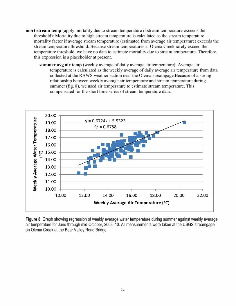
summer avg air temp (weekly average of daily average air temperature): Average air temperature is calculated as the weekly average of daily average air temperature from data collected at the RAWS weather station near the Olema streamgage.Because of a strong relationship between weekly average air temperature and stream temperature during summer (fig. 8), we used air temperature to estimate stream temperature. This compensated for the short time series of stream temperature data.

Figure 8. Graph showing regression of weekly average water temperature during summer against weekly average air temperature for June through mid-October, 2003–10. All measurements were taken at the USGS streamgage on Olema Creek at the Bear Valley Road Bridge.

25

stream temp threshold (stream temperature above which fish mortality increases): Literature values exist describing the effects of high stream temperature on coho physiology: • Lethal temperature=25.1 oC (Reiser and Bjornn, 1979, as cited in Brett, 1952). • Growth occurs 5–17 oC (Brungs and Jones, 1977). • Growth slowed considerably near 18 oC (Stein and others, 1972). • Growth ceases >20.3 oC (Bell, 1973). • Temperatures in the warmest tributaries containing juvenile coho were <18 oC

calculated from maximum weekly maximum temperatures or <16.7 oC calculated from maximum weekly average temperatures (Welch and others, 2001).

• Juvenile coho were most abundant in areas with temperatures 18–20 oC (Ebersole and others, 2009).

We use average weekly stream temperatures of >18 oC as the criterion for increased mortality. This happened only once during the period of record for this project (week 34, ending 07-26-2006). This year had good survival from early summer to smolting so any impact of high stream temperature was negligible. Consequently, we will model a small effect until more data documenting high effects of high stream temperatures become available.

stream temp mort factor (effect on fish mortality if weekly stream temperature exceeds the threshold): Because there is insufficient data to estimate the effect of temperature on coho mortality in Olema Creek, we included the value 0.01 as a placeholder in the model.

26

annual juv max (fraction of potential carrying capacity for fish realized in any particular year based on that year’s flow regime): This converter expresses the maximum carrying capacity during summer for each year as a function of flow. Higher summer flow is expected to increase habitat availability, which translates into higher capacity for fish (Burns, 1971; Bjornn and Reiser, 1991). It is expressed as the fraction of maximum fish capacity realized as a function of the number of weeks with minimum flow less than 0.2 ft3/s (fig. 9). Notably, this relationship was determined during the short period of record, which is a period of especially low flow since flow records began in 1895. Because we expressed the effect of low-flow conditions as a fraction of carrying capacity, the model can easily reflect a change in maximum carrying capacity that might result from restoration activities.

Figure 9. Graph showing fraction of maximum fish capacity realized as a function of the number of summer weekly low flows below 0.2 cubic feet per second (ft3/s) each year.

27

juvenile summer max (maximum potential summer carrying capacity for fish under ideal conditions): The maximum number of juveniles that can survive the summer in Olema Creek expresses the carrying capacity of the creek and density dependence of the fish population. We determined carrying capacity of Olema Creek by fitting Ricker and Beverton-Holt (B-H) recruitment curves (Guy and Brown, 2007) to redd (representing spawners) and smolt data (fig. 10). The Ricker curve was fit using the linear form of the Ricker equation (Guy and Brown, 2007):

ln(smolts/redds) = a – b(redds)

where a describes density-independent recruitment and b is the density-dependent coefficient. Next, we fit the B-H equation (Moussalli and Hilborn, 1986):

smolts = p(redds)/(1 + p/c(redds)) where p describes density-independent recruitment and c is the capacity parameter such that carrying capacity is p divided by c. We fit the B-H equation based on density-independent recruitment from the Ricker curve and finding c to minimize the summed deviation of observations from predicted values as recommended by Guy and Brown (2007). The best-fit B-H curve described carrying capacity as 4,673 fish (c=0.026) performed better than the Ricker curve based on sum of deviations (B-H=47; Ricker=1,326). The regression of predicted against observed using the B-H curve has r2 of 0.42. This analysis requires at least 20 data points to be reliable (Guy and Brown, 2007); therefore, we consider this to be a first approximation.

Figure 10. Graph showing comparisons among observed smolt counts and predicted smolts using Ricker and Beverton-Holt equations (Guy and Brown, 2007).

28

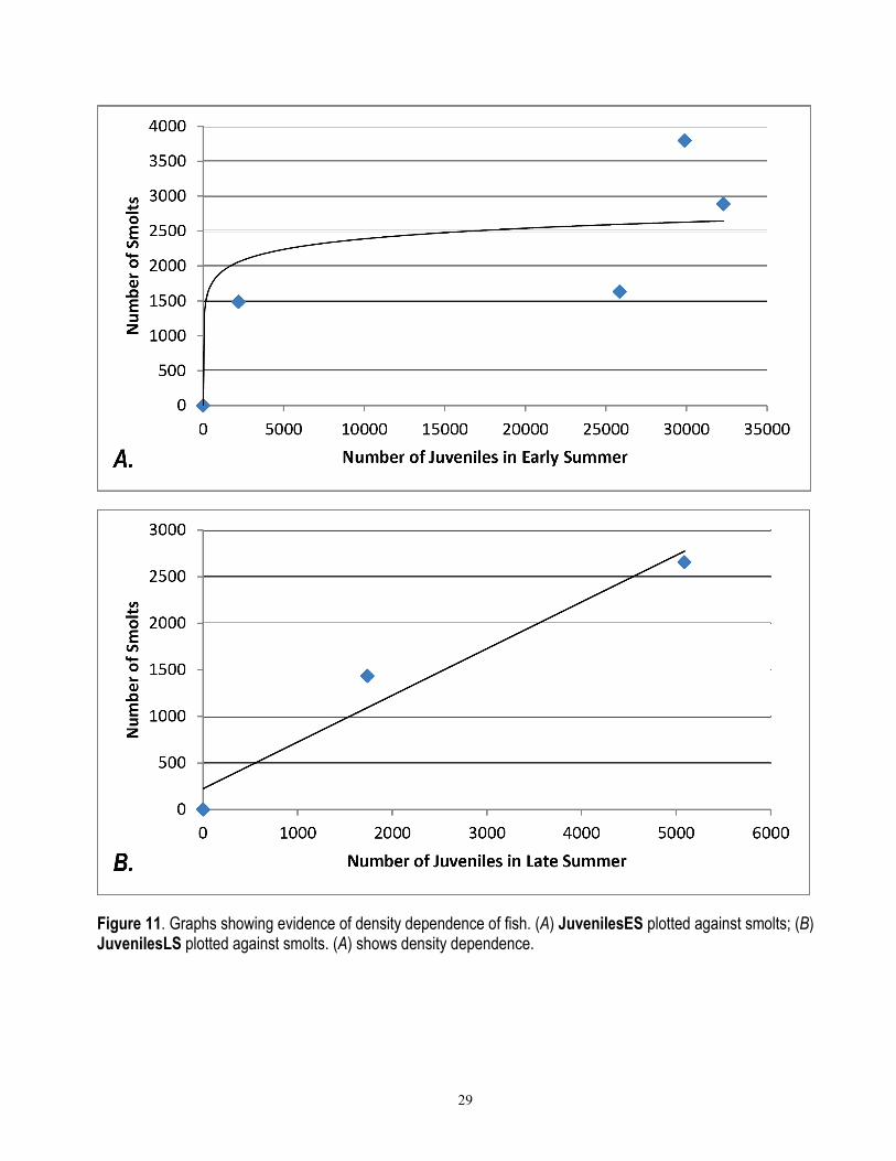
The carrying capacity determined from the B-H equation represents carrying capacity through the smolt stage. To calculate carrying capacity for juveniles, we divided 4,673 by 0.8 to account for 20 percent baseline mortality from juvenile to smolt (see base mortality wint spr2). The resulting capacity of 5,841 is higher than the highest corrected juvenile count of 5,088 for 2007–08 (table 1). The limited data from Olema Creek show the strongest evidence of density dependence during summer (fig. 11A) rather than during the second winter and spring (fig. 11B). However, these relationships are extremely weak, because a linear relationship has an equivalent r2 to the logarithmic relationship (0.68) in figure 11 A; and figure 11B has only 3 points, of which one is 0.0. Evidence of summer density dependence contradicts the Lagunitas Limiting Factors study (Stillwater Sciences, 2008), which concluded that there is no habitat carrying capacity effect in summer, but there is in winter. Perhaps this difference reflects the difference in flow regime between a dammed system (Lagunitas) with a mandated release of 6–8 ft3/s of water throughout the summer, and an unregulated system (Olema) that often becomes disconnected by the end of summer (Reichmuth and others, 2006). Moreover, density dependence of coho during summer has been observed by others, although the spatial scale at which it manifests varies with the ability of fish to move among habitat units (Ebersole and others, 2009). The default value for maximum number of juveniles used in the model is 4,673. This number can be interactively increased in the model to reflect improvements to habitat using the slider (see annual juv max).

Critical min summer flow count (stock that counts number of low-flow events) summer min flow (weekly minimum of average daily flow): This value is based on

streamflow measured at the Olema Creek streamgage. Data are input using a spreadsheet (appendix A).

summer critical flow threshold (stream flow below which juvenile mortality increases): The value is 0.2 ft3/s as measured at the Olema Creek streamgage. This value was chosen by comparing juvenile survival with the number of weeks below a range of low-flow values from 0.1 to 0.5 ft3/s. The value 0.2 ft3/s best explained years with low juvenile survival. Increased mortality may be due to reduction in habitat.

29

Figure 11. Graphs showing evidence of density dependence of fish. (A) JuvenilesES plotted against smolts; (B) JuvenilesLS plotted against smolts. (A) shows density dependence.

30

Juveniles in Late Summer to Smolts (Model Weeks 46–75)

Introduction (Winter-Spring2: mid-October through April) The third section of the model describes factors affecting survival of juveniles through fall and

winter until they become smolts and migrate to the ocean (fig. 12). Model terms, definitions, sources, confidence, and relationship to one another are given in table 2. This section includes the 29 weeks between mid-October and the end of April of the following year (abbreviated in model as “wint spr2” for second winter and spring; model weeks 46-74). During this stage, main threats to juvenile coho include displacement by high-flow events (Tschaplinski and Hartman, 1983; McMahon and Hartman, 1989; Nickelson and others, 1992; Giannico and Healey, 1998; Gallagher and others, 2012), and secondarily, predation (Mason, 1966; Hartman and others, 1982). Modeled factors affecting mortality include baseline mortality due to factors not explicitly modeled, density effects, high-flow events, and habitat factors that might help fish survive high flows. Inputs are weekly maximum values of average daily streamflow measured at the Olema Creek streamgage.

Mortality for the entire period is calculated in one step at the end. We include baseline mortality due to factors not modeled, density dependent mortality if fish numbers exceed a threshold representing carrying capacity as well as flow and habitat factors. As with other effects of streamflow, we have modeled the effects of high flow in winter as a function of the number of effects over a threshold. Mortality due to poor habitat is separated from density effects because habitat data are collected, and could eventually be used to define a relationship between habitat and mortality. At present, habitat data are collected during summer and are not particularly informative regarding winter conditions, but the monitoring protocol could change. The relationship between habitat and mortality is modeled as a threshold separating ‘good’ years from ‘bad;’ mortality is reduced if habitat is above the threshold, representing ‘good’ conditions. Because there is no evidence of effects other than baseline mortality in the data, other morality effects are included because they are hypothesized to be important and so the model user can experiment with them.

31

Figure 12. Diagram showing section of model describing survival of juveniles over second winter and spring until they become smolts from mid-October through April as it appears in Stella®.

32

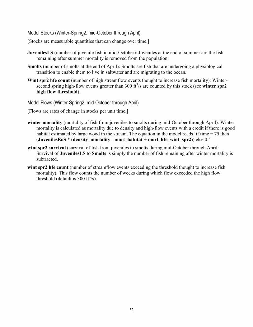
Model Stocks (Winter-Spring2: mid-October through April) [Stocks are measurable quantities that can change over time.]

JuvenilesLS (number of juvenile fish in mid-October): Juveniles at the end of summer are the fish

remaining after summer mortality is removed from the population.

Smolts (number of smolts at the end of April): Smolts are fish that are undergoing a physiological transition to enable them to live in saltwater and are migrating to the ocean.

Wint spr2 hfe count (number of high streamflow events thought to increase fish mortality): Winter-second spring high-flow events greater than 300 ft3/s are counted by this stock (see winter spr2 high flow threshold).

Model Flows (Winter-Spring2: mid-October through April) [Flows are rates of change in stocks per unit time.] winter mortality (mortality of fish from juveniles to smolts during mid-October through April): Winter

mortality is calculated as mortality due to density and high-flow events with a credit if there is good habitat estimated by large wood in the stream. The equation in the model reads ‘if time = 75 then (JuvenilesEoS * (density_mortality - mort_habitat + mort_hfe_wint_spr2)) else 0.’

wint spr2 survival (survival of fish from juveniles to smolts during mid-October through April: Survival of JuvenilesLS to Smolts is simply the number of fish remaining after winter mortality is subtracted.

wint spr2 hfe count (number of streamflow events exceeding the threshold thought to increase fish mortality): This flow counts the number of weeks during which flow exceeded the high flow threshold (default is 300 ft3/s).

33

Model Converters (Winter-Spring2: mid-October through April) These converters affect the rate of the model flow winter mortality, directly or by affecting

other converters or stocks. Converters that affect other converters or stocks are indented under the affected stock or converter.

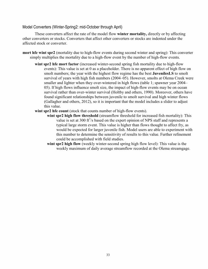
mort hfe wint spr2 (mortality due to high-flow events during second winter and spring): This converter

simply multiplies the mortality due to a high-flow event by the number of high-flow events.

wint spr2 hfe mort factor (increased winter-second spring fish mortality due to high-flow events): This value is set at 0 as a placeholder. There is no apparent effect of high flow on smolt numbers; the year with the highest flow regime has the best JuvenilesLS to smolt survival of years with high fish numbers (2004–05). However, smolts at Olema Creek were smaller and lighter when they over-wintered in high flows (table 1; spawner year 2004–05). If high flows influence smolt size, the impact of high-flow events may be on ocean survival rather than over-winter survival (Holtby and others, 1990). Moreover, others have found significant relationships between juvenile to smolt survival and high winter flows (Gallagher and others, 2012), so it is important that the model includes a slider to adjust this value.

wint spr2 hfe count (stock that counts number of high-flow events). wint spr2 high flow threshold (streamflow threshold for increased fish mortality): This

value is set at 300 ft3/s based on the expert opinion of NPS staff and represents a typical large storm event. This value is higher than flows thought to affect fry, as would be expected for larger juvenile fish. Model users are able to experiment with this number to determine the sensitivity of results to this value. Further refinement could be accomplished with field studies.

wint spr2 high flow (weekly winter-second spring high flow level): This value is the weekly maximum of daily average streamflow recorded at the Olema streamgage.

34

density mortality – (density-dependent mortality of juvenile fish during mid-October through April). Although there are no density effects on juveniles evident during winter in this dataset, density dependence has been indicated by data from Lagunitas Creek (Stillwater Sciences, 2008) and in Caspar and Pudding Creeks in Mendicino County (Gallagher and others, 2012). Density dependence is thought to exist more generally due to the need for habitat that provides protection from high-flow events (Tschaplinski and Hartman, 1983; McMahon and Hartman, 1989; Nickelson and others, 1992). To incorporate the potential for density-dependent mortality into the model, mortality is expressed as baseline mortality if juvenile number is less than the density threshold. Data show that at high numbers of juveniles, the regression slope of smolts against juveniles is nearly 0 (fig. 11A); therefore, mortality is calculated as the proportion of juveniles that are above the density threshold. The equation in the model reads ‘if JuvenilesEoS < density_threshold then base_mortality__wint_spr2 else ((JuvenilesEoS - density_threshold)/JuvenilesEoS).’

base mortality wint spr2 (mortality of fish from juveniles to smolts during mid-October through April due to factors not explicitly included in the model): Baseline mortality of over-wintering juveniles was set at 20 percent based on 80 percent survival seen in 2007–08 data (table 1) when juveniles were counted at the end of the summer, recruitment was below carrying capacity (B-H analysis), and there were no high-flow events. Additional data are needed to validate this relationship.

density threshold (carrying capacity of Olema Creek for juvenile coho): The carrying capacity of Olema Creek was estimated to be 4,673 using a B-H recruitment curve (see juv summer max).

35

mort habitat (applies increased fish mortality if the habitat index is below the threshold thought to increase fish mortality): Mortality due to habitat quality is modeled as a threshold effect. The threshold is set at the average habitat index value in the dataset and serves as a placeholder. The model equation reads ‘if habitat < habitat_threshold then mort_habitat_factor else 0.’

habitat index (index describing habitat quality during mid-October though April): The Olema dataset does not include a wide range of habitat values and data are collected during summer and only for reaches with water, an approach that may not accurately describe winter conditions. Data for length of pieces of large woody debris (LWD) in several size categories were recorded for selected reaches along the Olema Creek. We used the annual sum of lengths of largest LWD categories (rootwads, >50 cm, >20 cm, LWD jams) for all reaches as a creek-wide index of habitat quality. Because data were collected over different extents of the river in different years, the index is based on those reaches that were sampled every year. The index value is entered into the model using a spreadsheet (appendix A). Despite the weaknesses of the Olema Creek data, habitat quality has been shown to significantly affect winter survival (Bell, 2001), especially over a wide range of habitat change created by substantial stream manipulation (Solazzi and others, 2000; fig. 13).

mort habitat factor (effect on fish mortality if habitat quality is poor): The range of values for habitat in the available dataset is too small to see an effect. Consequently, this number is set at 0 and is a placeholder until more data are collected for Olema Creek.

habitat threshold (threshold of the habitat index below which fish mortality is thought to increase): The Olema Creek dataset does not include a wide range of habitat values. This value (400) is the average of the annual sums of length of LWD in the largest categories (rootwads, pieces >50 cm diameter, pieces >20 cm diameter, LWD jams) during the period of record.

36

Figure 13. Graph showing effect of winter habitat on winter survival of salmon. Data from Solazzi and others (2000).

37

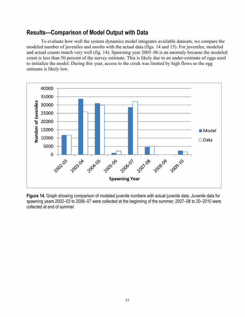
Results—Comparison of Model Output with Data To evaluate how well the system dynamics model integrates available datasets, we compare the

modeled number of juveniles and smolts with the actual data (figs. 14 and 15). For juveniles, modeled and actual counts match very well (fig. 14). Spawning year 2005–06 is an anomaly because the modeled count is less than 50 percent of the survey estimate. This is likely due to an under-estimate of eggs used to initialize the model. During this year, access to the creek was limited by high flows so the egg estimate is likely low.

Figure 14. Graph showing comparison of modeled juvenile numbers with actual juvenile data. Juvenile data for spawning years 2002–03 to 2006–07 were collected at the beginning of the summer; 2007–08 to 20–2010 were collected at end of summer.

38

The number of smolts produced is more uniform across years than is true of juveniles (fig. 15). For most years, the results match well, with modeled numbers higher in some years and actual data higher in others. Model results for spawning year 2005–06 are low, likely because of the difficulty in counting eggs as previously described. The estimate of smolts for spawning year 2006–07 was higher than the modeled number even though there were four high-flow events that were not accounted for in the model.

Overall, the model effectively describes available coho data from Olema Creek. Paired t-tests comparing modeled smolts and juveniles with data show no significant difference (p=0.452, smolts; p=0.548, juveniles). This is not a validation of the model, but merely indicates that the model explains the fish data using processes and factors thought to be important in determining fish survival.

Figure 15. Graph showing comparison of modeled smolt numbers with actual data, 2002–2010.

39

Potential Uses of Model This system dynamics model of Olema Creek is a synthesis of available data based on current

hypotheses regarding interactions between salmon and their environment. It is built to be easy to manipulate by park staff and others, and could be used for the following purposes:

• Validate model with future data: As monitoring data continue to accumulate, they will represent a wider range of environmental conditions, including new combinations of average events as well as more extreme events. By comparing modeled survival with monitored survival, the veracity of the model can be tested.

• Test sensitivity of results to parameter values: Parameters in the model are based on relationships developed from relatively short time series of data, literature values, or expert opinion. By changing parameters and re-running the model, the user can determine the sensitivity of model outcomes. Eventually, a formal sensitivity analysis could be conducted to determine which parameters have the greatest influence on fish survival.

• Public outreach: The model could be used as a teaching tool with a variety of audiences to explain how various factors interact to affect fish survival.

• Improve monitoring program and restoration activities: Outcomes from model validation and tests of sensitivity to parameters will likely suggest additional data needs, data that may not need to be collected, or more effective ways to collect data. Ultimately, the model could be used to redirect monitoring and restoration experimentation and be used as a tool to test potential scenarios for improving growth, survival, and production of juvenile salmon. Effectively monitoring habitat and understanding the potential for habitat availability to mitigate adverse flow conditions is an obvious need.

40

Model Limitations All models necessarily simplify reality. Users of this model should be aware of its limitations

and consider them when evaluating model outcomes. • Limits of conceptual model: The model reflects current thinking of NPS resource managers

regarding factors limiting coho production in the freshwater environment. While this conceptual model is based on direct experience and scientific evidence, the system is not perfectly understood and the model may change as more information accumulates.

• Short time series. The model is based on data collected over a very short period of time, which did not include the full range and combination of possible environmental conditions. Consequently, many relationships (for example mortality due to low DO or high temperature) could not be described because limiting conditions did not occur during the sampled time period. These factors were included in the model with placeholder values so model users can experiment with potential values. In addition, the short time series constrains even parameterized relationships to be based on few observations.

• Not all important factors were measured: Datasets were not available to describe the condition of environmental factors suspected to be important. Examples include habitat condition during winter and predation. Some of these cases were addressed using literature values (for example, limiting levels of DO).

• Interaction terms were not included: For example, the effects of flow depend on the availability of refugia created by large woody debris. Future versions of the model would benefit from adding this complexity.

• Unforeseen or unpredictable changes: It is likely that unforeseen limiting factors will arise as the environment changes and produces novel combinations of conditions. An example might be shifts in the timing of high or low flows such that they affect different life stages of fish than at present (Stewart and others, 2004). Changes in abundance and distribution of invasive species and exotic diseases are other potential ecosystem stressors. Moreover, present assumptions may not hold in the future. For example, we do not know how fish may alter their life cycle to adapt to future environments. A small fraction of the coho population already do not adhere to the 3-year life cycle.

Acknowledgments We would like to thank the following staff of NPS and USGS who participated in discussions

leading to the structure of the model, provided data, and otherwise supported its completion: Sarah Allen, Monica Bueno, Sarah Carlisle, Marie Denn, Rob Carson, Brannon Ketchum, Michelle O’Herron, Marcus Koenen, and Tamara Williams. We would also like to thank the USGS Status and Trends Program for funding this project.

41

References Cited Andrews, E.D., 1983, Entrainment of gravel from naturally sorted riverbed material: Geological Society

of America Bulletin, v. 94, p. 1,225-1,231. Beidler, W.M., and Nickelson, T.E., 1980, An evaluation of the Oregon Department of Fish and

Wildlife standard spawning fish survey system for coho salmon: Oregon Department of Fish and Wildlife Information Report Series, Fisheries Number 80-9.

Bell, E.A., 2001, Survival, growth, and movement of juvenile coho salmon (Oncorhynchus kisutch) over-wintering in alcoves, backwaters, and main channel pools in Prairie Creek, California: Humboldt State University, Arcata, California, M.S. thesis.

Bell, E.A., and Duffy, W.G., 2007, Previously undocumented two-year freshwater residency of juvenile coho salmon in Prairie Creek, California: Transactions of the American Fisheries Society, v. 136, p. 966–970.

Bell, M.C., 1973, Fisheries handbook of engineering requirements and biological criteria: Portland, Oregon, U.S. Army Corps of Engineers Division, 353 p.

Bjornn, T.C., and Reiser, D.W., 1991, Habitat requirements of salmonids in streams, in Meehan, W.R., ed., Influence of forest and rangeland management of salmonid fishes and their habitat: Bethesda, Md., American Fisheries Society Special Publication 19.

Bovee, K.D., 1978, Probability-of-use criteria for the family Salmonidae: Fort Collins, Colorado., U.S. Fish and Wildlife Service, Instream Flow Information Paper No. 4.

Brett, J.R., 1952, Temperature tolerance in young Pacific salmon, genus Oncorhynchus: Journal of the Fisheries Research Board of Canada, v. 9, p. 265–309.

Brett, J.R., and Blackburn, J.M., 1981, Oxygen requirements for growth of young coho (Oncorhynchus kisutch) and sockeye (O. nerka) salmon at 15 ºC: Canadian Journal of Fisheries and Aquatic Science, v. 38, p. 399–404.

Brungs, W.A., and Jones, B.R., 1977, Temperature criteria for freshwater fish—Protocol and procedures: Duluth, Minnesota, Environmental Protection Agency Environmental Research Laboratory, EPA-600/3-77-061.

Bugert, R.M., Bjornn, T.C., and Meehan, W.R., 1991, Summer habitat use by young salmonids and their responses to cover and predators in a small south east Alaska stream: Transactions of the American Fisheries Society, v. 120, p. 474–485.

Burns, J.W., 1971, The carrying capacity for juvenile salmonids in some northern California streams: California Fish and Game, v. 57, p. 44–57.

Carlisle, S.J., Reichmuth, M., Dedrick, A., and Rodoni, A., 2013, Long-term coho salmon and steelhead trout monitoring in coastal Marin County 2010 annual monitoring progress report: Point Reyes Station, Calif., Point Reyes National Seashore Association, Coho and Steelhead Monitoring Program Report prepared for California Department of Fish and Wildlife.

Chamberlain, C.D., Martin, A.C., and Petros, P.P., 2007, Trinity River biological monitoring of channel rehabilitation sites—A pre-construction baseline habitat evaluation: Arcata, California, U.S. Fish and Wildlife Service, Arcata Fish and Wildlife Office, Arcata Fisheries Technical Report TR 2007-07.

Davison, R.C., Breese, W.P., Warren, C.E., and Doudoroff, P., 1959, Experiments on the dissolved oxygen requirements of cold-water fishes: Sewage and Indutrial Waste, v. 31, p. 950–966.

Dettinger, M., 2011, Climate change, atmospheric rivers, and floods in California–A multimodel analysis of storm frequency and magnitude changes: Journal of the American Water Resources Association, v. 47, p. 514–523.

Dunne, T., and Leopold, L.B., 1978, Water in Environmental Planning: San Francisco, California, W.H. Freeman, 818 p.

42

Ebersole, J.L., Colvin, M.E., Wigington, Jr., P.J., Leibowitz, S.G., Baker, J.P., Church, M.R., Compton, J.E., and Cairns, M.A., 2009, Hierarchical modeling of late-summer weight and summer abundance of juvenile coho salmon across a stream network: Transactions of the American Fisheries Society, v. 138, p. 1,138-1,156.

Ettlinger, E., Kranz, C., Rohr, F., and Andrew, G., 2006, Juvenile salmonid population monitoring report, Lagunitas Creek, Marin County, California, fall 2005: Corte Madera, California, Marin Municipal Water District, accessed September 25, 2013, at http://www.marinwater.org/documents/MMWD_Juv_Report_2005.pdf.

Ford, F.A., 1999, Modeling the environment—An introduction to system dynamics models of environmental systems: Washington, D.C., Island Press.

Gallagher, S.P., Adams, P.B., Wright, D.W., and Collins, B.W., 2010, Performance of spawner survey techniques at low abundance levels: North American Journal of Fisheries Management, v. 30, p. 1,086–1,097.

Gallagher, S.P., Thompson, S., and Wright, D., 2012, Identifying factors limiting coho salmon to inform stream restoration in coastal Northern California: California Fish and Game, v. 98, p. 185–201.

Gallagher, S.P., Thompson, S., and Wright, D.W., 2013a, Coastal Mendocino County salmonid life cycle and regional monitoring—Monitoring status and trends for 2012: Fortuna, California, California State Department of Fish and Wildlife, Coastal Watershed Planning and Assessment Program, 2011–12 Administrative Report, 47 p.

Gallagher, S.P., Thompson, S., and Wright, D.W., 2013b, Coastal Mendocino County salmonid life cycle and regional monitoring—Monitoring status and trends for 2013: Fortuna, California, California State Department of Fish and Wildlife, Coastal Watershed Planning and Assessment Program, 2012–13 Administrative Report, 47 p.

Gallagher, S.P., and Wright, D.W., 2012, Coastal Mendocino County salmonid life cycle and regional monitoring—Monitoring status and trends for 2011: Fortuna, California, California State Department of Fish and Wildlife, Coastal Watershed Planning and Assessment Program.

Giannico, G.R., and Healey, M.C., 1998, Effects of flow and food on winter movements of juvenile coho salmon: Transactions of the American Fisheries Society, v. 127, p. 645–651.

Groot, C., and Margolis, L., 1991, Pacific salmon life histories: Vancouver, University of British Columbia Press.

Guy, C.S., and Brown, M.L., eds., 2007, Analysis and interpretation of freshwater fisheries data: Betheseda, Md., American Fisheries Society.

Harvey, B.C., 1987, Susceptibility of young-of-the-year fishes to downstream displacement by flooding: Transactions of the American Fisheries Society, v. 116, p. 851–855.

Heggenes, J., and Traaen, T., 1988, Downstream migration and critical water velocities in stream channels for fry of four salmonid species: Journal of Fish Biology, v. 32, p. 717–727.

Herrmann, R.C., Warren, C.E., and Doudoroff, P., 1962, Influence of oxygen concentration on the growth of juvenile coho salmon: Transactions American Fishery Society, v. 91, p. 155–167.

Hicks, B.J., Beschta, R.L., and Harr, R.D., 1991, Long-term changes in streamflow following logging in western Oregon and associated fisheries implications: Water Resources Bulletin, v. 27, p. 217–226.

Holtby, L.B., Andersen, B.C., and Kadowski, R.K., 1990, Importance of smolt size and early ocean growth to interannual variability in marine survival of coho salmon (Oncorhynchus kisutch): Canadian Journal of Fisheries and Aquatic Sciences, v. 47, p. 2,181–2,194.

Johnston, N.T., Irvine, J.R., and Perrin, C.J., 1987, Instream indexing of coho salmon (Oncorhynchus kisutch) escapement in French Creek, British Columbia: Vancouver, British Columbia, Fisheries and Oceans, Canadian Technical Report of Fisheries and Aquatic Sciences, no. 1573.

43

Madej, M.A., 2012, Analysis of trends in climate, streamflow, and stream temperature in North Coastal California, in Medley, C.N., Patterson, Glenn, and Parker, M.J., eds., 2011, Observing, studying, and managing for change—Proceedings of the Fourth Interagency Conference on Research in the Watersheds: U.S. Geological Survey Scientific Investigations Report 2011–5169, 202 p., http://pubs.usgs.gov/sir/2011/5169/.

Mason, J.E., 1966, The migrant dipper—A trap for downstream-migrating fish: The Progressive Fish-Culturist, v. 28, p. 96–102.

McMahon, T.E., 1983, Habitat suitability index models—Coho salmon: Washington, D.C., U.S. Fish and Wildlife Service, FWS/OBS-82/10.49.

McMahon, T.E., and Hartman, G.F., 1989, Influence of cover complexity and current velocity on habitat use by juvenile coho salmon (Oncorhynchus kisutch): Canadian Journal of Fisheries and Aquatic Sciences, v. 46, p. 1,551–1,557.

Montgomery, D.R., Buffington, J.M., Peterson, N.P., Schuett-Hames, D., and Quinn, T.P., 1996, Stream-bed scour, egg burial depths, and the influence of salmonid spawning on bed surface mobility and embryo survival: Canadian Journal of Fisheries and Aquatic Sciences, v. 53, p. 1,061—1,070.

Mousalli, E., and Hilborn, R., 1986, Optimal stock size and harvest rate in multistage life history models: Canadian Journal of Fisheries and Aquatic Sciences, v. 43, p. 135-141.

Nickelson, T.E., Rodgers, J.D., Johnson, S.L., and Solazzi, M.F., 1992, Seasonal changes in habitat use by juvenile coho salmon (Oncorhynchus kisutch) in Oregon coastal streams: Canadian Journal of Fisheries and Aquatic Sciences, v. 49, p. 783–789.

Ottaway, E.M., and Clarke, A., 1981, A preliminary investigation into the vulnerability of young trout (Salmo trutta) and Atlantic salmon (Salmo salar) to downstream displacement by high water velocities: Journal of Fish Biology, v. 19, p. 135–145.

Quinn, T.P., 2005, The Behavior and Ecology of Pacific Salmon and Trout: Seattle, Washington, University of Washington Press.

Raleigh, R.F., Hickman, T., Soloman, R.C., and Nelson, P.C., 1984, Habitat suitability information— Rainbow trout (Onchorhynchus mykiss): Washington, D.C., U.S. Fish and Wildlife Service, FWS/OBS-82/10.60.

Reichmuth, M., Ketcham, B.J., Leising, K., and Craig, B., 2006, Olema Creek watershed summary monitoring report, Marin County, California. 1997–2005: Point Reyes, California, National Park Service, PORE/NR/WR/06-02., 90 p. plus appendixes.

Reiser, D.W., and Bjornn., T.C., 1979, Influence of forest and rangeland management of anadromous fish habitat in the western United States and Canada—Habitat requirements of anadromous salmonids: Portland, Oregon, U.S. Department of Agriculture, Pacific Northwest Research Station, Forest Service General Technical Report PNW-96, 54 p.

Shapovalov, L., and Berrian, W., 1940, An experiment in hatching silver salmon (Oncorhynchus kisutch) eggs in gravel: Transactions of the American Fisheries Society, v. 69, p. 135–140.

Shapovalov, L., and Taft, A.C., 1954, The life histories of the steelhead rainbow trout (Salmo gairdneri gairdneri) and silver salmon (Oncorhychus kisutch) with special reference to Waddell Creek, California, and recommendations regarding their management: Sacramento, Calif., State of California Department of Fish and Game, Fish Bulletin no. 98.

Sheppard, J.D., and Johnson, J.H., 1985, Probability–of-use for depth, velocity, and substrate by subyearling coho salmon and steelhead in Lake Ontario tributary streams: North American Journal of Fisheries Management, v. 5, p. 277–282.

44

Shirvell, C.S., 1990, Role of instream rootwads as juvenile coho salmon (Oncorhynchus kisutch) and steelhead trout (O. mykiss) cover habitat under varying streamflows: Canadian Journal of Fisheries and Aquatic Sciences, v. 47, p. 852–861.

Solazzi, M.F., Nickelson, T.E., Johnson, S.L., and Rodgers, J.D., 2000, Effects of increasing winter rearing habitat on abundance of salmonids in two coastal Oregon streams: Canadian Journal of Fishery and Aquatic Science, v. 57, p. 906–914.

Stein, R.A., Reimers, P.E., and Hall, J.D., 1972, Social interaction between juvenile coho (Oncorhynchus kisutch) and fall chinook salmon (O. tshawytscha) in Sixes River, Oregon: Journal of the Fisheries Research Board of Canada, v. 29, p. 1,737–1,748.

Stewart, I.T., Cayan, D.R., and Dettinger, M.D., 2004, Changes in snowmelt runoff timing in western North America under a ‘business as usual’ climate change scenario: Climatic Change, v. 62, p. 217–232.

Stillwater Sciences, 2008, Lagunitas limiting factor analysis, limiting factors for coho salmon and steelhead—Final report: Point Reyes Station, Berkeley, California, Stillwater Sciences for Marin Resource Conservation District, Point Reyes Station.

Tschaplinski, P.J., and Hartman, G.F., 1983, Winter distribution of juvenile coho salmon (Oncoryhnchus kisutch) before and after logging in Carnation Creek, British Columbia, and some implications for overwinter survival: Canadian Journal of Fisheries and Aquatic Sciences, v. 40, p. 452–461.

Welch, H.H., Hodgson, G.R., Harvey, B.C., and Roche, M.E., 2001, Distribution of juvenile coho salmon in relation to water temperature in tributaries of the Mattole River, California: North American Journal of Fisheries Management, v. 21, p. 464–470.

45

Appendix A. Input Spreadsheet Format Input to the system dynamic simulation model of coho salmon in Olema Creek is in the form of

an Excel® workbook, with each year entered on a separate spreadsheet. There are no data for spawning year 2008–09 because adult fish were unable to return due to low flow. Initial eggs, beginning of spawn, end of spawn and the habitat index (Habitat) are used to initialize the model for each year. The habitat index is the annual sum of largest LWD categories (rootwads, >50 cm, >20 cm, LWD jams) for all reaches. Spring high flow (ft3/s), summer minimum flow (ft3/s), summer average air temperature (oC), and winter-second spring high flow (ft3/s) are weekly values, and vary with each time step. The weekly time steps begin during the first week of December and continue through the end of April of the second spring and are counted in the last column of the spreadsheet. Column headings must exactly match the spelling and capitalization of corresponding elements in the model. Tinted cells indicate estimate values.

initial

eggs

beg of

spawn

end of

spawn Habitat

spring

high flow

summer

min flow

summer avg

air temp

wint spr2

high flow

51876 5 12 397 184.32 0 0 0 1

5.35 0 0 0 2

2.28 0 0 0 3

3.43 0 0 0 4

115.7 0 0 0 5

99.99 0 0 0 6

133.79 0 0 0 7

177.29 0 0 0 8

69.49 0 0 0 9

22.28 0 0 0 10

22.16 0 0 0 11

110.29 0 0 0 12

17.02 0 0 0 13

11.25 0 0 0 14

23.15 0 0 0 15

58.41 0 0 0 16

17.42 0 0 0 17

9.24 0 0 0 18

6.15 0 0 0 19

29.13 0 0 0 20

21.41 0 0 0 21

30.45 0 0 0 22

60.02 0 0 0 23

17.42 0 0 0 24

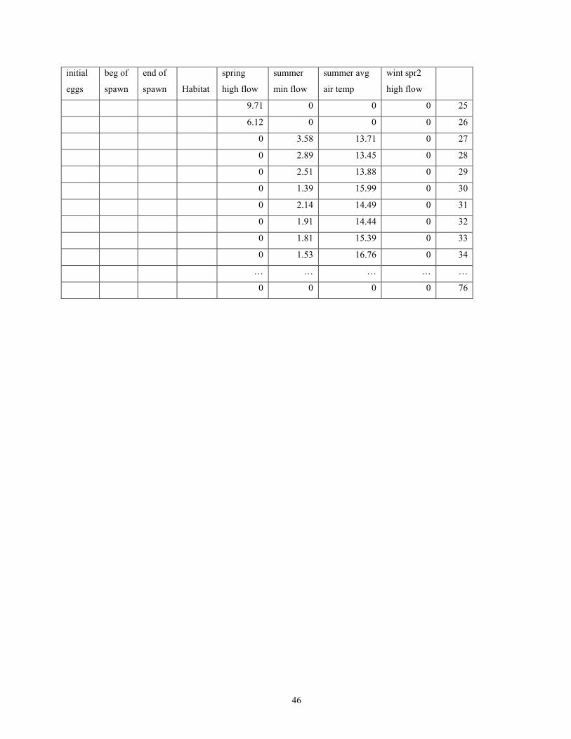
46

initial

eggs

beg of

spawn

end of

spawn

Habitat

spring

high flow

9.71

summer

min flow

0

summer avg

air temp

0

wint spr2

high flow

0

25

6.12 0 0 0 26

0 3.58 13.71 0 27

0 2.89 13.45 0 28

0 2.51 13.88 0 29

0 1.39 15.99 0 30

0 2.14 14.49 0 31

0 1.91 14.44 0 32

0 1.81 15.39 0 33

0 1.53 16.76 0 34

… … … … …

0 0 0 0 76

47

Appendix B. Acquiring and Running Model The Olema Creek system dynamic simulation model and input file can be downloaded from

http://pubs.usgs.gov/ofr/2014/1131. Running the model requires the Stella® software program produced by isee systems™. A free

version of the software, the isee Player™, will allow the user to alter the default values using the slider bars on the interactive interface and enter new data by creating a new input spreadsheet. The isee Player™ can be downloaded from the isee systems website at http://www.iseesystems.com. The free version of the software will not allow the user to modify the model structure.

A video-based tutorial that shows how to run the model is available at http://www.werc.usgs.gov/ProjectSubWebPage.aspx?SubWebPageID=7&ProjectID=229.

Orientation to Stella® Examples in the following section are based on version 10.0, but apply to all versions through

10.0.3. After opening the software and the model file, the user will notice four tabs on the left side of the

application window. The top tab is the Interface view where the user can run the model and also easily experiment with it by changing the parameters between each run. Next is the Map tab, which shows a simplified diagram of the model. Symbols include boxes for stocks, arrows with valves for flows, circles for converters, and clouds for stocks that are no longer counted in the model. This view can be used to sketch the model as part of the model development process. Next is the Model tab, which describes the nuts and bolts of the model using the same symbols as described for the map tab (fig. B1). Finally, under the Equation tab, the user will find all of the equations that implement the model.

Figure B1. Screen capture showing contents of Model tab in Stella® showing stocks, flows, and converters.

48

Double click on any stock, converter, or flow icon in the Model tab to see the default value, equation, and documentation for that element of the model. For example, upon clicking on the fry flow event threshold converter in the Model tab, a “properties window” opens showing the default value of 200. Documentation describing units and source is found by clicking on the tab with the page symbol at the bottom of the pop-up page. In this example, the source is expert knowledge (fig. B2). Mortality due to scour events is an example based on data and mortality due to stream temperature is an example of an equation. In this case, stream temperature is predicted from air temperature because the data record for stream temperature is much shorter than the record for air temperature. Consequently, average weekly stream temperature is this function of average weekly air temperature. On the Interface tab, the default value is displayed on each slider and the documentation can be viewed by clicking on the question mark (fig. B3).

Figure B2. Screen capture showing display of contents and documentation for converters in Model tab.

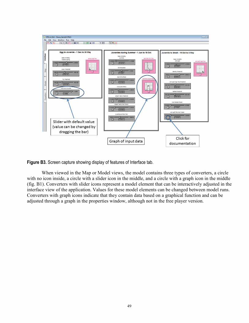
49

Figure B3. Screen capture showing display of features of Interface tab.

When viewed in the Map or Model views, the model contains three types of converters, a circle with no icon inside, a circle with a slider icon in the middle, and a circle with a graph icon in the middle (fig. B1). Converters with slider icons represent a model element that can be interactively adjusted in the interface view of the application. Values for these model elements can be changed between model runs. Converters with graph icons indicate that they contain data based on a graphical function and can be adjusted through a graph in the properties window, although not in the free player version.

50

Model Input File An example input file is presented in appendix A. In this spreadsheet, there is a tab for every

year for which we have data from Olema Creek. Each tab has an initial “eggs” value, the week during which spawning began, the week when the last redd was observed to be built, a habitat index value to describe habitat quality, and environmental variables.

Running the Model The model can be run from several tabs, but the Interface tab is a good place to start. In order to

run the model, the user must import the data from the input file. Steps include: go to the Edit tab; click on Import Data; choose one time rather than establishing persistent links; browse to the input file; open; and then choose the year. Open the drop down menu for Worksheet Name to see all of the years with data and choose one. The data orientation should have headings across the top and values down the columns (fig. B4). Click OK. A dialog box informs the user that the data have been successfully imported. Click OK. Go to the Run tab and click Run. The graph and table should begin filling with results.

Figure B4. Screen capture showing process for importing data into Stella® model.

51

The table begins at the beginning of the time steps and runs through all of the weeks of the model. Total mortality from spring (first section of the model) is applied in one step and the remaining fish are transferred from Eggs to JuvenilesBoS in week (time step) 26. The JuvenileBoS stock declines until the end of summer when the remaining fish are transferred to the next stock and then all of the final mortality is applied at the end of the time steps. Other values can be added to the table by double-clicking on the table, selecting a value from the list and using the double arrows to move it to the selected column (fig. B5). To remove a value, the user does the reverse.

Figure B5. Screen capture showing process for adding variables to the table display.

52

The graph displays the same variables that appear on the table and each variable has its own scale (fig. B6). This is done so the user can actually see the relatively small numbers towards the end of the run. The scale automatically adjusts for each model run. To modify the graph, the user double-clicks on the graph and uses the same steps to add and remove variables as were used on the table.

Figure B6. Screen capture showing graphical output from Stella® model.

53

The user can run through all of the years in the same way or use the interface to alter the values and see how changes in some of the parameters might affect the outcome of the model. One way to do this is to take base mortality factor spring, for example, and increase it to simulate disease in the system. The change can be made by moving the slider by dragging it with the mouse and then re-running the model. The default value can be restored by clicking the U (for ‘undo’) button, which will appear next to the question mark on the slider. Graphical input data also can be modified by double-clicking on the graph and then clicking above or below the original line to change the graph, and then re-running the model (fig. B7).

Figure B7. Screen capture showing process for changing the data in a graphical time series.

54

A sensitivity analysis can be accomplished using the Sensi-Specs feature. Under the Run tab, clicking on Sensi-Specs enables the user to pick a value for which to assess sensitivity of the model (fig. B8). For example, one could choose base mortality wint spr2 and select it, highlight it by clicking on it, then enter the desired number of runs. For example, choose 3 and pick the beginning and ending numbers 0.1 and 0.3, to bracket the default value of 0.2. After clicking on Set, the software will distribute those values evenly (if incremental is selected) over the number of runs requested. Click OK.

Figure B8. Screen capture showing process for setting up the Sensi Specs feature of the model.

55

To set up the graph for Sensi-Specs the user will double click on the graph (fig. B9). In this case, Comparative graph should be the default value. Perhaps the most interesting number is the number of smolts, so select that variable. Because smolts come out at the end of the model run, it is most efficient to only display the last steps. The user should choose page 1 of the graph and click OK.

Figure B9. Screen capture showing process for setting up the graphical display of Sensi Specs results.

56

To set up the table for Sensi-Specs, the user will double click on the table. Again, smolts will likely be added to the table, Comparative table is appropriate, as is page one. Click OK.

To run Sensi-Specs, the user will go to the Run tab. This time there will be an S in front of Run, indicating that Sensi-Specs will be run. After clicking on Run-S, results from 3 runs will appear on the graph and table (fig. B10). These results indicate how sensitive the model is to changes in base mortality wint spr2. The graphs and tables can be cleared by clicking on the dynamite symbol. In the Olema Creek model each year of data has different numbers of eggs and environmental conditions so sensitivity to various factors will vary with year.

Figure B10. Screen capture showing graphical output from Sensi Specs feature of the model.

Stella software has many more features and capabilities than described here, but these instructions should enable the user to run the model and do some rudimentary exploration. Tutorials are also available at the isee systems™ website (http://www.iseesystems.com).

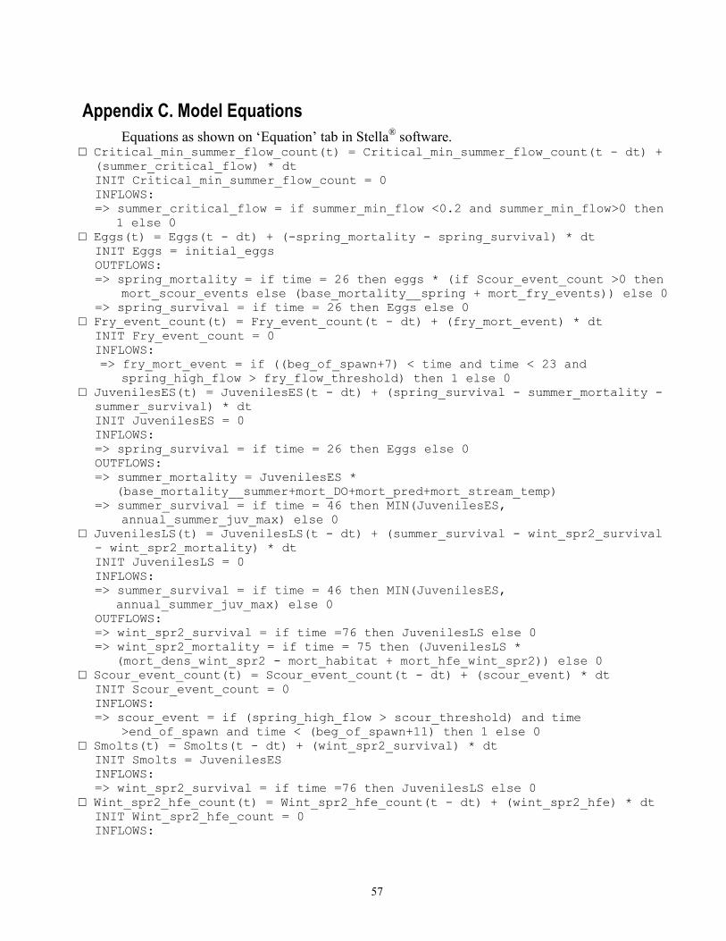
57

Appendix C. Model Equations Equations as shown on ‘Equation’ tab in Stella® software.

□ Critical_min_summer_flow_count(t) = Critical_min_summer_flow_count(t - dt) + (summer_critical_flow) * dt INIT Critical_min_summer_flow_count = 0 INFLOWS: => summer_critical_flow = if summer_min_flow <0.2 and summer_min_flow>0 then

1 else 0 □ Eggs(t) = Eggs(t - dt) + (-spring_mortality - spring_survival) * dt

INIT Eggs = initial_eggs OUTFLOWS: => spring_mortality = if time = 26 then eggs * (if Scour_event_count >0 then

mort_scour_events else (base_mortality__spring + mort_fry_events)) else 0 => spring_survival = if time = 26 then Eggs else 0

□ Fry_event_count(t) = Fry_event_count(t - dt) + (fry_mort_event) * dt INIT Fry_event_count = 0 INFLOWS: => fry_mort_event = if ((beg_of_spawn+7) < time and time < 23 and

spring_high_flow > fry_flow_threshold) then 1 else 0 □ JuvenilesES(t) = JuvenilesES(t - dt) + (spring_survival - summer_mortality -

summer_survival) * dt INIT JuvenilesES = 0 INFLOWS: => spring_survival = if time = 26 then Eggs else 0 OUTFLOWS: => summer_mortality = JuvenilesES *

(base_mortality__summer+mort_DO+mort_pred+mort_stream_temp) => summer_survival = if time = 46 then MIN(JuvenilesES,

annual_summer_juv_max) else 0 □ JuvenilesLS(t) = JuvenilesLS(t - dt) + (summer_survival - wint_spr2_survival

- wint_spr2_mortality) * dt INIT JuvenilesLS = 0 INFLOWS: => summer_survival = if time = 46 then MIN(JuvenilesES,

annual_summer_juv_max) else 0 OUTFLOWS: => wint_spr2_survival = if time =76 then JuvenilesLS else 0 => wint_spr2_mortality = if time = 75 then (JuvenilesLS *

(mort_dens_wint_spr2 - mort_habitat + mort_hfe_wint_spr2)) else 0 □ Scour_event_count(t) = Scour_event_count(t - dt) + (scour_event) * dt

INIT Scour_event_count = 0 INFLOWS: => scour_event = if (spring_high_flow > scour_threshold) and time

>end_of_spawn and time < (beg_of_spawn+11) then 1 else 0 □ Smolts(t) = Smolts(t - dt) + (wint_spr2_survival) * dt

INIT Smolts = JuvenilesES INFLOWS: => wint_spr2_survival = if time =76 then JuvenilesLS else 0

□ Wint_spr2_hfe_count(t) = Wint_spr2_hfe_count(t - dt) + (wint_spr2_hfe) * dt INIT Wint_spr2_hfe_count = 0 INFLOWS:

58

=> wint_spr2_hfe = if(wint_spr2_high_flow > wint_spr2_high_flow_threshold) then 1 else 0

○ annual_summer_juv_max = if Critical_min_summer_flow_count>0 then juvenile_summer_max * (-.129*LN(Critical_min_summer_flow_count)+.5155) else juvenile_summer_max

○ base_mortality__spring = 0.77 ○ base_mortality__summer = 0.007 ○ base_mortality__wint_spr2 = 0.2 ○ beg_of_spawn = 2 ○ density_threshold_wint_spr2 = 4673 ○ DO_threshold = 4.5 ○ end_of_spawn = 9 ○ fry_flow_threshold = 200 ○ habitat = 502 ○ habitat_threshold = 400 ○ initial_eggs = 23726 ○ juvenile_summer_max = 5841 ○ mort_dens_wint_spr2 = if JuvenilesLS < density_threshold_wint_spr2 then ○

base_mortality__wint_spr2 else ((JuvenilesLS - ○ density_threshold_wint_spr2)/JuvenilesLS)

○ mort_DO = if (1.542 * LN(summer_min_flow)+6.617) < (DO_threshold) then ○ mort_DO_factor else 0 ○ mort_DO_factor = 0.01 ○ mort_fry_events = if Fry_event_count > 0 then (4.46 * ln(Fry_event_count) +

10.93)/100 else 0 ○ mort_habitat = if habitat > habitat_threshold then mort_habitat_factor else 0 ○ mort_habitat_factor = 0 ○ mort_hfe_wint_spr2 = Wint_spr2_hfe_count*wint_spr2_hfe_mort_factor ○ mort_pred = if summer_min_flow < pred_threshold then mort_pred_factor else 0 ○ mort_pred_factor = 0.01 ○ mort_scour_events = 0.98 ○ mort_stream_temp = if (0.672 * summer_avg_air_temp + 5.532) >

stream_temp_threshold then stream_temp_mort_factor else 0 ○ pred_threshold = 0.01 ○ scour_threshold = 1090 ○ spring_high_flow = GRAPH(TIME) ○ stream_temp_mort_factor = 0.01 ○ stream_temp_threshold = 18 ○ summer_avg_air_temp = GRAPH(TIME) ○ summer_critical_flow_threshold = 0.2 ○ summer_min_flow = GRAPH(TIME) ○ wint_spr2_hfe_mort_factor = 0 ○ wint_spr2_high_flow = GRAPH(TIME) ○ wint_spr2_high_flow_threshold = 300

Publishing support provided by the U.S. Geological SurveyPublishing Network, Tacoma Publishing Service Center

For more information concerning the research in this report, contact the Director, Forest and Rangeland Ecosystem Science Center

U.S. Geological Survey 777 NW 9th St., Suite 400 Corvallis, Oregon 97330 http://fresc.usgs.gov/

Woodw

ard and others—U

sers’ Guide to System D

ynamics M

odel Describing Coho Salm

on Survival in Olema Creek—

Open-File Report 2014–1131

ISSN 2331-1258 (online)http://dx.doi.org/10.3133/ofr20141131