uses of generalized convexity and generalized monotonicity in economics

Uses of Generalized Convexity and

Generalized Monotonicity in Economics

Reinhard John1

Department of EconomicsUniversity of BonnAdenauerallee 24-42

53113 Bonn, Germanyemail: [email protected]

June 2004

1This paper has been prepared as a chapter for the Handbook of GeneralizedConvexity and Generalized Monotonicity, edited by N. Hadjisavvas, S. Komlosi,and S. Schaible. I am grateful to Luigi Brighi since it has benefited from mycollaboration with him.

CONTENTS 1

Contents

1 Introduction 2

1.1 Georgescu-Roegen’s Local Preferences . . . . . . . . . . . . . . 2

1.2 Wald’s Equilibrium Existence Proof . . . . . . . . . . . . . . . 4

1.3 An Outline of this Chapter . . . . . . . . . . . . . . . . . . . . 6

2 Consumer Theory 7

2.1 Preference and Utility . . . . . . . . . . . . . . . . . . . . . . 7

2.2 Demand and Revealed Preference . . . . . . . . . . . . . . . . 13

2.3 Nontransitive Preference . . . . . . . . . . . . . . . . . . . . . 18

3 General Equilibrium Theory 28

3.1 Variational Inequalities and Economic Equilibrium . . . . . . 28

3.2 Distribution Economies . . . . . . . . . . . . . . . . . . . . . . 31

3.3 Exchange Economies . . . . . . . . . . . . . . . . . . . . . . . 36

References 45

1 INTRODUCTION 2

1 Introduction

Probably the first use of generalized monotonicity in economics was madealmost seventy years ago. Even more remarkable, it occured independentlyand almost at the same time in two seminal articles. The one, by Georgescu-Roegen [13], dealt with the concept of a local preference in consumer theory,the other, by Wald [45], contained the first rigorous proof of the existenceof a competitive general equilibrium. We shall outline their contributions inthis introduction, borrowing some insights from the illuminating papers byShafer [42] and Kuhn [32].

1.1 Georgescu-Roegen’s Local Preferences

Imagine a consumer who considers alternative consumption bundles in aneighborhood of some given vector x ∈ R

l+ that describes the amounts of l

consumption goods initially given. The consumer is able to distinguish thepossible directions in which he can move away from x according to his taste.More precisely, there are three kinds of directions: Preference, nonpreference,and indifference. This idea had been already formalized in [2] by postulatingthe existence of a (row) vector g(x) ∈ R

l such that a direction v ∈ Rl is a

preference (resp. nonpreference, indifference) direction if and only if

g(x)v > 0 (resp. < 0, = 0). (1)

It should be emphasized that these comparisons are supposed to be possibleonly locally. The consumer may not be able to compare x with a bundle ythat is very different from x. In addition, the vector g(x) typically varieswith x (otherwise, one would obtain the special case of a global preferencerepresenting perfect substitutes).

Assume now that x is contained in some given set X ⊆ Rl+ that represents

the consumer’s feasible bundles. Georgescu-Roegen calls x an ”equilibriumposition or a point of saturation” relative to X if no direction away from xto any other alternative y in X is one of preference, i.e. if

g(x)(y − x) ≤ 0 for all y ∈ X. (2)

Thus, x is an equilibrium consumption bundle if, in modern terminology, xis a solution to the Stampacchia variational inequality problem with respectto g on X.2

2Notice the reverse inequality compared to the usual definition. This convention isemployed throughout the chapter.

1 INTRODUCTION 3

By assuming that the consumer always selects such an equilibrium out ofa set of alternatives provided it exists, Georgescu-Roegen’s concept of a localpreference could be a foundation of a demand theory. However, for that heneeded existence of an equilibrium bundle, at least in budget sets determinedby prices and income.

Since he also wanted the equilibrium to be stable, he formulated anotherassumption that he called the ”principle of persisting nonpreference ”:

If the consumer moves away from an arbitrary bundle x to a bundlex+∆x such that ∆x is not a preference direction, then ∆x is a nonpreferencedirection at x + ∆x. Formally stated, this principle says

g(x)∆x ≤ 0 implies g(x + ∆x)∆x < 0, (3)

or, by denoting x + ∆x = y,

g(x)(y − x) ≤ 0 implies g(y)(y − x) < 0. (4)

Clearly, this property is nothing else than strict pseudomonotonicity of g.3

In a sequel contribution, Georgescu-Roegen [14] employed a slightly dif-ferent formulation of his principle of persisting nonpreference:

An indifference or nonpreference direction remains one of indifference ornonpreference if the consumer extends his consumption according to thatdirection, or, formally,

g(x)(y − x) ≤ 0 implies g(y)(y − x) ≤ 0, (5)

i.e. g is pseudomonotone.Georgescu-Roegen has also shown that the set of equilibrium points rela-

tive to a feasible set X is convex. In addition, he observed that these equilib-ria are, in modern terminology, solutions to the Minty variational inequalityproblem with respect to g on X.

More surprisingly, Georgescu-Roegen [14] proved the existence of a con-sumption equilibrium in a simplex. Of course, he assumed continuity of gwhich, as we know, is sufficient for the existence of a solution to the Stam-pacchia variational inequality problem with respect to g. However, he didnot use any advanced argument like Brouwer’s fixed point theorem. Instead,he succeeded by induction on the dimension of the simplex. For that, heused pseudomonotonicity of g. Actually, it is the same idea that Wald em-ployed in [45] in order to prove the existence of a competitive equilibrium ofa production economy.

3In this chapter, all notions of (generalized) monotonicity are defined in the sense ofgeneralizing a nonincreasing real valued function of one real variable.

1 INTRODUCTION 4

1.2 Wald’s Equilibrium Existence Proof

Wald considered a general equilibrium model of a production economy wherethe production sector is characterized by fixed input coefficients. Its origin isthe simplification of Walras’ famous production equations in [7], [8], [46], and[39]. We shall present here a slightly different version of his model that is dueto Kuhn [32]. For a historically closer but nevertheless modern treatment werefer to Hildenbrand [18].

The economic environment is described by m pure factors of productioni = 1, ...,m which are available in fixed positive amounts r = (r1, ..., rm)and which can be used to produce n final commodities j = 1, ..., n. Theproduction of one unit of commodity j requires aij ≥ 0 units of the primaryresource i, i.e. the production sector is characterized by the input coefficientmatrix A = (aij)m×n.

Assume that price vectors p = (p1, ..., pn) ≥ 0 for final commodities andq = (q1, ..., qm) ≥ 0 for factors are given. Then the output vector x =(x1, ..., xn) ≥ 0 maximizes profits if unit costs are greater or equal thanoutput price, equality being implied by a nonzero output quantity, i.e. if

qA ≥ p and (qA − p)x = 0, (6)

where prices are represented by row vectors, quantities by column vectors.All factor markets are in (free disposal) equilibrium if on every market

demand is less than or equal to supply, equality being implied by a positivefactor price, i.e. if

Ax ≤ r and q(Ax − r) = 0. (7)

By the duality theory of linear programming, it is well known that (6) and(7) are equivalent to the statement that x and q solve the dual problems

max px subject to x ≥ 0 and Ax ≤ r (8)

andmin qr subject to q ≥ 0 and qA ≥ p, (9)

or, equivalently, that p, q, and x satisfy the conditions

Ax ≤ r, qA ≥ p, and px = qr. (10)

It remains to close the model by an equilibrium condition for the productmarkets. According to Schlesinger’s modification of Cassel’s equations thisis accomplished by assuming the existence of an inverse demand function f ,i.e. by

p = f(x), (11)

1 INTRODUCTION 5

which means that the vector x of final commodities is demanded if and onlyif their prices are given by f(x).

It was essentially the system of conditions (6), (7), and (11) for whichWald proved the existence of a solution (p∗, q∗, x∗). His proof is based on thefollowing assumptions:

(W1) For every j ∈ {1, ..., n} there exists i ∈ {1, ...,m} such that aij > 0.

(W2) f : Rn+ −→ R

n++ is continuous.

(W3) For every x, x′ ∈ Rn+ such that x 6= x′,

f(x)(x′ − x) ≤ 0 implies f(x′)(x′ − x) < 0.

Assumption (W1) guarantees that the production possibilities are bounded,i.e. X = {x ≥ 0 |Ax ≤ r} is bounded. This implies for any p ≥ 0 theexistence of an element x∗ ∈ X that maximizes px on X, i.e. the primallinear programming problem mentioned above has the optimal solution x∗.

By the duality theorem of linear programming, it follows that the dualproblem can be solved by some q∗. Consequently, (p, q∗, x∗) satisfies (6) and(7) but not necessarily p = f(x∗).

Thus, we have to find a vector x∗ that maximizes f(x∗)x on X, i.e. welook for x∗ ∈ X such that for all x ∈ X

f(x∗)x ≤ f(x∗)x∗, (12)

or, equivalently,f(x∗)(x − x∗) ≤ 0. (13)

In modern terminology, we have to solve a variational inequality problem.Assumption (W2) guarantees the existence of a solution which, as Kuhn[32] has shown, can be proved by applying Kakutani’s fixed point theorem.However, this result was not available to Wald.

On the other hand, we have not used (W3) which states that f is strictlypseudomonotone. Obviously, this assumption is not necessary for an exis-tence proof. What was its use for Wald?

The crucial point is that strict pseudomonotonicity of f ensures a uniquesolution to the variational inequality problem with respect to f on every con-vex subset of X. It is this consequence that enabled Wald to prove existenceby induction on the number n of final commodities.

Remember that Georgescu-Roegen proceeded in the same way. An ele-mentary induction proof that resembles their contributions has been given in[27] for the general case of a pseudomonotone variational inequality problemon a compact and convex subset of a finite dimensional Euclidean space.

1 INTRODUCTION 6

1.3 An Outline of this Chapter

In the sequel, we shall present some uses of generalized concavity and gener-alized monotonicity in the same two fields of research that contain the con-tributions by Georgescu-Roegen and Wald, i.e. consumer theory and generalequilibrium theory. Of course, it is not claimed that there are no applica-tions in other fields as, for example, game theory.4 However, since we wantto focus on generalized monotonicity, we have selected those which seem tobe more relevant to that part of the subject. The reader who is interested inmore applications of generalized concavity is referred to [4].

Part 2 deals with consumer theory. The first section introduces the clas-sical approach which employs the notion of a utility function that representsa transitive preference relation. We stress the role played by quasiconcavityor pseudoconcavity of that function.

Section 2.2 considers the central concept of demand. It is shown thatthe demand relation derived from a transitive preference displays generalizedmonotonicity properties that are, in the economic literature, well known asaxioms of revealed preference theory.

In the final section of this part, we extend the classical approach by study-ing nontransitive preferences (a convenient abbreviation for ”not necessarilytransitive” which would be the correct expression). If these relations are con-vex (resp. semistrictly or strictly convex), various generalized monotonicityproperties of demand arise quite naturally. Like in the case of transitive pref-erences, these are related to well known revealed preference axioms. However,in order to obtain a fully satisfactory revealed preference theory, some openproblems have still to be solved. The section concludes with the first ordercharacterization of pseudomonotone continuously differentiable demand thatwill be used in the two final sections of this chapter.

Part 3 deals with general equilibrium theory. Its first section points outthe relationship to variational inequalities (see e.g.[10]). In particular, therelevance of pseudomonotone excess demand to the stability of an equilib-rium is recognized by its representability as a solution to a Minty variationalinequality problem. The main insight can be easily visualized by a ball in apseudoconvex landscape (see Figure 1 below).

If the ball moves according to the force of gravity, it will move awayfrom any point like A or C towards B. As a rest point with respect to themovement of the ball, B represents an equilibrium of the physical system. Itis unique if the landscape is strictly pseudoconvex. If there is a flat region

4See e.g. the excellent survey by Harker and Pang in [15].

2 CONSUMER THEORY 7

A

B

C

Figure 1

around B, the set of equilibria is at least convex.Notice that these conclusions are not valid if the landscape is only (semi-

strictly) quasiconvex. Indeed, that case allows a vanishing slope at pointslike A or C such that these could be equilibria too (although not stableones if the quasiconvexity is semistrict). On the other hand, observe thata (strictly) convex landscape is not needed for stability. This observationis important since an economic system may satisfy conditions that ensurea pseudomonotone excess demand but fails to fulfill stronger requirementsimplying monotonicity.

The final Sections 3.2 and 3.3 provide two standard examples for a gen-eral equilibrium model. We shall not present the most general versions. Forexample, set-valued excess demand as well as production will not be con-sidered.5 This seems to be acceptable in order to convey the main idea assimply as possible.

While Section 3.1 points out the importance of a pseudomonotone excessdemand function for a well-behaved economic model, Sections 3.2 and 3.3investigate conditions that ensure this property. It will be argued there thatdistributional assumptions are appropriate in order to reach that goal. In thisrespect, the presentation will follow closely the contributions by Hildenbrand[17] and Jerison [25].

2 Consumer Theory

2.1 Preference and Utility

We consider an economy with a finite (typically large) number l of consump-tion goods. A vector x = (xi)

li=1 ∈ R

l+ describing the consumption of xi

units of commodity i for i = 1, ..., l is called a consumption bundle.

5For such an exposition of general equilibrium theory, [36] is highly recommended.

2 CONSUMER THEORY 8

The traditional approach (see e.g.[36]) assumes that a consumer’s tasteis characterized by a binary relation � on the consumption set R

l+ with the

following two basic properties.

Completeness: ∀x, y ∈ Rl+ : x � y ∨ y � x .

Transitivity: ∀x, y, z ∈ Rl+ : x � y ∧ y � z ⇒ x � z .

The relation � is called the consumer’s preference. For x, y ∈ Rl+, x � y is

interpreted as ”x is at least as good as y” or ”x is weakly preferred to y”.While transitivity follows naturally from this interpretation, completenessmeans that the consumer is able to compare any two commodity bundles.Observe that the latter property implies that � is reflexive, i.e. x � x for allx ∈ R

l+.

There are two other relations that can be derived from � .The strict preference � is defined by

x � y : ⇔ x � y ∧ ¬y � x (14)

and interpreted as ”x is better than y”.If x � y but not x � y, x and y are called to be indifferent which is

denoted by x ∼ y. Obviously, x ∼ y if and only if x � y and y � x.Usually, it is also assumed that � is continuous, i.e. � (as a subset of

R2l+) is closed in R

2l+.

Continuous preferences are precisely those relations on Rl+ which can be

represented by a continuous real valued function on Rl+, i.e. we obtain

Proposition 1 A binary relation � is a continuous preference if and onlyif there is a continuous function u : R

l+ → R such that for all x, y ∈ R

l+

x � y ⇔ u(x) ≥ u(y). (15)

Proof It is obvious that a relation � satisfying (15) for a continuous functionu is complete, transitive, and continuous. A proof of the reverse implicationcan be found in [12]. �

A real valued function u that satisfies (15) is called a utility representa-tion (or utility function) of the preference � . Observe that any monotonetransformation of u also represents �, i.e. u is far from being unique. In thesequel, we suppose that u is some fixed continuous utility function represent-ing the continuous preference � .

In many cases it is natural to assume that the consumption of goods aredesirable, at least if they are consumed together. This is made precise by

Definition 1 The preference � (resp. the utility function u) is called

2 CONSUMER THEORY 9

(1) monotone if for all x, y ∈ Rl+, x � y implies x � y (resp. u(x) >

u(y)),

(2) strictly monotone if for all x, y ∈ Rl+, x > y implies x � y (resp.

u(x) > u(y)).6

There is a weaker assumption that allows the presence of some ”bads”.

Definition 2 The preference � (resp. the utility function u) is called locallynonsatiated with respect to X ⊆ R

l+ at x ∈ X if for every neighborhood N

(w.r.t. X) of x there is y ∈ N such that y � x (resp. u(y) > u(x)). � (resp.u) is locally nonsatiated if it is locally nonsatiated with respect to R

l+ at every

x ∈ Rl+.

The ultimate goal of consumer theory is to derive a useful theory ofdemand from the hypothesis that a consumer maximizes utility on (convex)budget sets. For that, the following basic notions of convexity turn out to beimportant.

Definition 3 The preference � is called

(1) convex, if x � y implies λx + (1 − λ)y � y

(2) semistrictly convex, if x � y implies λx + (1 − λ)y � y

(3) strictly convex, if x � y implies λx + (1 − λ)y � y

for all x, y ∈ Rl+ such that x 6= y and all λ ∈]0, 1[.

Obviously, (3) implies (2) and, by continuity of �, (2) implies (1). Thelatter implication is proved in [12] where a somewhat different terminologyis used. The notation employed here seems to be more appropriate becauseof the following straightforward relationship(cf.[4]).

Proposition 2 The preference � is (strictly, semistrictly) convex if and onlyif the utility representation u of � is (strictly, semistrictly) quasiconcave.

The economic rationale for convexity are ”nonincreasing (decreasing)rates of substitution”. This property is easily explained for the case of twocommodities. Consider a monotone and convex preference on R

2+. Convex-

ity means that the set X of all bundles that are weakly preferred to someconsumption bundle x is convex, i.e. it typically looks like X in Figure 2below.

6x � y means xi > yi for i = 1, ...l, and x > y means x ≥ y and x 6= y.

2 CONSUMER THEORY 10

1

2

x

y

X

Figure 2

The boundary of X consists of all bundles that are indifferent to x. Com-pare now the amount of good 2 that would compensate the consumer forconsuming one unit less of good 1 at the two points x and y. By convexity,it cannot be larger at y than at x (it is actually smaller at y if the prefer-ence is strictly convex). The quite intuitive interpretation is that additionalconsumption is less valuable if the quantity already consumed is larger.

What is added to convexity if the preference is semistrictly convex? Ananswer is provided by the following characterization.

Proposition 3 Let the preference � be convex. Then � is semistrictly con-vex if and only if for every convex subset X of R

l+ the preference � is locally

nonsatiated with respect to X at any x ∈ X that is not a global satiationpoint of X, i.e. at any x ∈ X such that there is y ∈ X with y � x.

Proof Let � be semistrictly convex and let X be a convex subset of Rl+.

Assume that x, y ∈ X such that y � x. Since λy +(1−λ)x � x for arbitrarysmall λ > 0 there is z ∈ X with z � x in every neighborhood of x. Thus, �is locally nonsatiated w.r.t. X at x.

In order to prove the converse, assume that � is not semistrictly convex,i.e. there are x, y ∈ R

l+ and µ ∈ ]0, 1[ such that x � y and y � µx+(1−µ)y =

z. It will be shown that y � zλ = λx + (1− λ)y for all λ ∈ [0, µ] (see Fig. 3).

Observe that x � y � z implies that x � zλ since otherwise, by convexityof �, z � x. From x � zλ it follows, again by convexity of �, that z � zλ

and, by transitivity, y � zλ.


µz = z

zλ

y

x

Figure 3

Consequently, � is locally satiated at y with respect to the line segment[y, x] although y is not a global satiation point of that convex set. �

The most important implication of a convex preference is the convexity(or uniqueness in case of strictly convex preferences) of the set of utilitymaximizers on a convex set. This property is crucial for the proof of theexistence of a market equilibrium. Moreover, it characterizes continuous(strictly) convex preferences as shown by

Proposition 4 Let u be a continuous utility function. Then

(1) u is quasiconcave if and only if for every convex subset X of Rl+ the

set X∗ = {x∗ ∈ X | ∀x ∈ X : u(x∗) ≥ u(x)} is convex.

(2) u is strictly quasiconcave if and only if for every convex subset X ofR

l+ there is at most one x∗ ∈ X such that u(x∗) ≥ u(x) for all x ∈ X.

Proof (1) Let u be quasiconcave and let X be an arbitrary convex subsetof R

l+. If x1, x2 ∈ X∗, then u(x1) ≥ u(x2) and, by quasiconcavity of u,

u(λx1 + (1 − λ)x2) ≥ u(x2) ≥ u(x) for all λ ∈ ]0, 1[ and all x ∈ X, i.e.λx1 + (1 − λ)x2 ∈ X∗.

In order to prove the converse, assume that u is not quasiconcave, i.e.there are x1, x2 ∈ R

l+ and µ ∈ ]0, 1[ such that u(x1) ≥ u(x2) and u(µx1 +

(1 − µ)x2) < u(x2). Define λ1, λ2 by

λ1 = max{λ ∈ [0, µ]| u(λx1 + (1 − λ)x2) ≥ u(x2)},

λ2 = min{λ ∈ [µ, 1]| u(λx1 + (1 − λ)x2) ≥ u(x2)}

(see Figure 4 below).By continuity of u, λ1 and λ2 exist. Furthermore, λ1 < µ < λ2. Thus,

for X = {λx1 + (1 − λ)x2 | λ1 ≤ λ ≤ λ2} we obtain X∗ = {λ1x1 + (1 −λ1)x2, λ2x1 + (1 − λ2)x2}. Since X∗ is not convex, (1) is proved.


u(x )1

u(x )2

λ1 λ20 1 λµ

Figure 4

(2) Let u be strictly quasiconcave and let X be an arbitrary convex subsetof R

l+. If x1, x2 ∈ X maximize u on X, then u(x1) = u(x2). It follows that

x1 = x2 since otherwise u( 12x1 + 1

2x2) > u(x2) = u(x1), i.e. x1 and x2 would

not maximize u on X.Now, assume that u is not strictly quasiconcave, i.e. there are x1, x2 ∈ R

l+

and µ ∈ ]0, 1[ such that x1 6= x2, u(x1) ≥ u(x2), and α := u(µx1 + (1 −µ)x2) ≤ u(x2). If there are µ1 ∈ [0, µ[ and µ2 ∈ ]µ, 1] such that u(µ1x1 +(1−µ1)x2), u(µ2x1 +(1−µ2)x2) > α, then u is not quasiconcave and we canapply part (1). Otherwise, either u(λx1 + (1− λ)x2) ≤ α for all λ ∈ [0, µ] oru(λx1+(1−λ)x2) ≤ α for all λ ∈ [µ, 1]. In the first case, x2 and µx1+(1−µ)x2

maximize u on X = {λx1 + (1 − λ)x2 | 0 ≤ λ ≤ µ}. In the second case,µx1 + (1 − µ)x2 and x1 maximize u on X = {λx1 + (1 − λ)x2 | µ ≤ λ ≤ 1}.Since in both cases there are two maximizers, (2) is proved. �

Let us now assume that the utility function u is differentiable. In thatcase it is desirable to determine a utility maximizing consumption bundleby a simple first order condition. In general, however, we only obtain thefollowing separate necessary and sufficient conditions.

Proposition 5 Let u be differentiable and let X be a convex subset of Rl+.

Then, for x∗ ∈ X the condition

(N) ∂u(x∗)(x − x∗) ≤ 0 for all x ∈ X

is necessary, and the condition

(S) ∂u(x)(x∗ − x) ≥ 0 for all x ∈ X

is sufficient for x∗ to maximize u on X.7

7∂u(x) denotes the Jacobian matrix of u at x, i.e. ∂u(x) = ∇u(x)T .


Proof If x∗ maximizes u on X, then for any x ∈ X such that x 6= x∗ andany λ ∈ [0, 1] the inequality u(x∗ + λ(x − x∗)) − u(x∗) ≤ 0 holds. Hence,

∂u(x∗)(x − x∗) = limλ→0

1

λ[ u(x∗ + λ(x − x∗)) − u(x∗) ] ≤ 0, (16)

which proves that (N) is necessary.In order to show that (S) is sufficient, assume that x∗ does not maximize

u on X, i.e. there exists x ∈ X such that u(x) > u(x∗). By the mean valuetheorem there exists α ∈ ]0, 1[ such that

∂u(x + α (x∗ − x))(x∗ − x) = u(x∗) − u(x) < 0.

For x = x + α (x∗ − x) it follows that x∗ − x = (1 − α)(x∗ − x) and,consequently, ∂u(x) 1

1−α(x∗ − x) < 0. Thus, we obtain, ∂u(x)(x∗ − x) < 0

which contradicts (S). �

Condition (N) means that x∗ is a solution to the Stampacchia variationalinequality problem with respect to ∇u on X and condition (S) means that x∗

is a solution to the Minty variational inequality problem with respect to ∇uon X (see [31]). Clearly, (N) is a simpler condition than (S) since it requiresknowledge of the gradient of u only at x∗. Therefore, we would be in a nicesituation if u would have the property that (N) implies (S).

It is known (see [26]) that (N) implies (S) for any convex subset X of Rl+

if and only if the gradient map of u is pseudomonotone, i.e. if

∂u(x)(y − x) ≤ 0 implies ∂u(y)(y − x) ≤ 0 (17)

for all x, y ∈ Rl+.

It is also known that pseudomonotonicity of the gradient map is equivalentto pseudoconcavity of u. Put differently, the pseudoconcave utility functionsare precisely those functions for which (N) characterizes a utility maximizingelement for every convex subset of R

l+.

Fortunately, the difference between pseudo- and quasiconcavity is notlarge. Indeed, as shown in [9], if the gradient of u does not vanish on anopen and convex domain X, then u is pseudoconcave on X if and only if uis quasiconcave on X.

2.2 Demand and Revealed Preference

Let p = (p1, ..., pl) � 0 be a market price vector for the various consumptiongoods and let the consumer’s wealth be given by w > 0. Then his budget setconsists of all bundles x ∈ R

l+ that are not more expensive than w, i.e.

B(p, w) = {x ∈ Rl+ | px ≤ w}, (18)


where the price vector p is always considered as a row vector.The utility maximization hypothesis states that the consumer chooses a

consumption bundle x∗ ∈ B(p, w) such that

u(x∗) ≥ u(x) for all x ∈ B(p, w). (19)

The set of all such x∗ is called the consumer’s demand at the price vectorp and wealth w. Since B(λp, λw) = B(p, w) for all λ > 0, one can representall possible budget sets by restricting the wealth to be equal to one. Putdifferently, p is interpreted as the vector of the price-income ratios. Thus,the demand relation Du ⊆ R

l++ × R

l+ derived from the utility function u is

defined by

(p, x) ∈ Du : ⇔ x ∈ B(p) ∧ ∀y ∈ B(p) : u(x) ≥ u(y) (20)

where B(p) = {x ∈ Rl+ | px ≤ 1}.

Clearly, Du can be equivalently described as a set-valued mapping fromR

l++ into R

l+, i.e. Du(p) = {x ∈ R

l+ | (p, x ) ∈ Du} for each p ∈ R

l++.

What properties of Du can be deduced from u? An answer is providedby

Proposition 6 Let u be continuous. Then the following properties can bederived:

(1) Du is an upper hemicontinuous and compact-valued correspondence, i.e.Du(p) 6= ∅ for all p ∈ R

l++ and for any sequence (pn, xn) ∈ Du such

that pn converges to p there is a subsequence of (xn) which convergesto x ∈ Du(p).

(2) If u is locally nonsatiated, then the budget identity pDu(p) = 1 holdsfor every p, i.e. px = 1 for all x ∈ Du(p).Moreover, Du satisfies the Generalized Axiom of Revealed Preference(GARP), i.e. for any (p1, x1), ..., (pn, xn) ∈ Du the inequalities

pi(xi+1 − xi) ≤ 0 for i = 1, ..., n − 1

imply that pn(x1 − xn) ≥ 0.

(3) If u is quasiconcave, then Du is convex-valued.

(4) If u is strictly quasiconcave, then Du(p) contains only one element, i.e.Du can be identified with a continuous function from R

l++ into R

l+.


Moreover, Du satisfies the Strong Axiom of Revealed Preference (SARP),i.e. for any (p1, x1), ..., (pn, xn) ∈ Du the inequalities

pi(xi+1 − xi) ≤ 0 for i = 1, ..., n − 1

and x1 6= xn imply that pn(x1 − xn) > 0.

Proof (1) Since the budget sets are compact, continuity of u implies thatDu(p) is nonempty and compact for each p. The budget correspondence Bfrom R

l++ into R

l+ is obviously continuous. Hence, by the maximum theorem

(see [5]), Du is upper hemicontinuous.(2) If px < 1 there is a neighborhood N of x such that pN < 1. Local

nonsatiation implies the existence of y ∈ N with u(y) > u(x). Since py ≤ 1,x does not maximize u on B(p).From pi(xi+1 − xi) ≤ 0 it follows that pixi+1 ≤ pixi = 1. Hence, xi+1 ∈B(pi) and thus u(xi) ≥ u(xi+1). By assumption, this inequality holds fori = 1, ..., n − 1. Consequently, u(x1) ≥ u(x2) ≥ ... ≥ u(xn−1) ≥ u(xn). Ifone would have pn(x1 − xn) < 0 or, equivalently, pnx1 < pnxn = 1, then,by local nonsatiation, x1 6∈ Du(pn) contradicting u(x1) ≥ u(xn). Therefore,pn(x1 − xn) ≥ 0.

(3) This follows immediately from Proposition 4 (1).(4) The first part follows immediately from Proposition 4 (2).As in the proof of (2), the inequalities pi(xi+1 −xi) ≤ 0 for i = 1, ..., n−1

imply that u(x1) ≥ ... ≥ u(xn). By strict quasiconcavity of u, x1 6= xn impliesthe existence of λ ∈ ]0, 1[ such that u(λx1 + (1 − λ)xn) > u(xn). Since xn

maximizes u on B(pn), λx1 + (1− λ)xn cannot be a bundle in B(pn). Hence,by convexity of B(pn), x1 6∈ B(pn), i.e. pnx1 > 1. Since pnxn = 1, it followsthat pnx1 > pnxn, i.e. pn(x1 − xn) > 0. �

It is obvious that SARP implies GARP but that the reverse is not true.For example, if p, x1, x2 are chosen such that x1 6= x2 and px1 = px2, thenD = {(p, x1), (p, x2)} satisfies GARP but not SARP.

While SARP was introduced by Houthakker [21], GARP has been for-mulated by Varian [44] as equivalent to the following condition of cyclicalconsistency which is due to Afriat [1]:

For any (p1, x1), ..., (pn, xn) ∈ Du the inequalities

pi(xi+1 − xi) ≤ 0 for i = 1, ..., n (mod n)

imply that pixi+1 = pixi for i = 1, ..., n (mod n).Afriat has also shown that any finite demand relation D = {(pi, xi) ∈

Rl++ × R

l+ | pixi = 1 for i = 1, ..., k} is cyclically consistent if and only if


there exist real numbers λ1, ..., λk > 0 such that

k (mod k)∑

i=1

λipi(xi+1 − xi) ≥ 0. (21)

Put differently, by setting qi = λipi for i = 1, ..., k, the transformeddemand relation D′ = {(qi, xi) | i = 1, ...k} is cyclically monotone. It is easyto see that any demand relation which is transformable (in the sense above)into a cyclically monotone one satisfies GARP. Indeed, pi(xi+1 − xi) ≤ 0 for

i = 1, ...n− 1 impliesn−1∑

i=1

λipi(xi+1 −xi) ≤ 0 ≤n(mod n)

∑

i=1

λipi(xi+1 −xi). Hence,

λnpn(x1 − xn) ≥ 0. Since λn > 0, pn(x1 − xn) ≥ 0.With regard to the above equivalences, it seems to be quite appropriate to

denote the generalized monotonicity property described by GARP as cyclicpseudomonotonicity. Actually, this term was first used by Daniilidis andHadjisavvas [11] for a general set-valued mapping displaying that property.8

Analogously, SARP might be called strict cyclic pseudomonotonicity sinceit generalizes the property that

n(mod n)∑

i=1

pi(xi+1 − xi) > 0 (22)

if xi 6= xi+1 for at least one i = 1, ..., n(mod n).Observe that if the utility function is neither locally nonsatiated nor

strictly quasiconcave, no generalized monotonicity property can be deduced.For example, a constant utility function u is even semistrictly quasiconcavebut puts no restriction on demand since Du(p) = B(p) for all p.

An important question is now whether the properties of Du that werededuced from certain properties of u in Proposition 6 actually characterizedemand relations derived from utility maximization. For example, if D :R

l++ −→ R

l+ is a continuous demand function satisfying the budget identity

and SARP, does there exist a continuous, locally nonsatiated, and strictlyquasiconcave utility function u such that Du = D?

Such questions are typically posed in the theory of revealed preferencethat tries to replace conditions on unobservable characteristics as preferenceand utility by conditions on the (in principle) observable demand relation.The main concepts are introduced by

8To be precise, GARP means that −D−1

u, where D−1

udenotes the set-valued mapping

corresponding to the inverse demand relation, is cyclically pseudomonotone in the senseof Daniilidis and Hadjisavvas.


Definition 4 A demand relation D ⊆ Rl++ × R

l+ is rationalized by a utility

function u (or by the corresponding preference relation) if D ⊆ Du. If actuallyD = Du, we say that u strongly rationalizes D.

While the concept of rationalizability should be interpreted as a consis-tency of the ”demand observations” with an underlying utility that is max-imized, strong rationalizability corresponds to a characterization of demandrelations derived from the utility maximization hypothesis.

Unfortunately, demand functions derived from a continuous and strictlyquasiconcave utility function (even if it is locally nonsatiated) cannot becharacterized by SARP. This can be seen from the following example due toHurwicz and Richter [22] and depicted in Figure 5 below.

x

2

1

Figure 5

For any budget line given by p, x = D(p) is chosen as the point for whichthe budget line is tangent at x to the curve on which x is located. Obviously,D satisfies the budget identity and is continuous. Since it is not difficultto verify that this demand function can be derived from maximizing an up-per semicontinuous utility function it satisfies SARP. However, as shown byHurwicz and Richter [22], it cannot be strongly rationalized by a continuousutility function.

Of course, as Houthakker [21] has already observed, if additional assump-tions (e.g. D is ”income Lipschitzian” and satisfies a boundary condition)are satisfied, then strict rationalizability by a continuous, monotone, andstrictly quasiconcave utility function is possible, see e.g. [34]. On the other


hand, these conditions are not necessary. To summarize, there is no way tocharacterize strong rationalizability of a demand function by a continuous,locally nonsatiated, and strictly quasiconcave utility function.

However, with regard to the weaker requirement of rationalizability, thereis a remarkable result due to Afriat [1] and reformulated by Varian [44].

Proposition 7 For a finite demand relationD = {(p1, x1), ..., (pk, xk)} ⊆ R

l++ × R

l+ the following properties are equiva-

lent:

(i) D can be rationalized by a locally nonsatiated utility function.

(ii) D satisfies the budget identity and GARP.

(iii) D can be rationalized by a continuous, monotone, and concave utilityfunction.

Proof See [44]. �

By the equivalence of (i) and (iii), if a finite demand relation can be ratio-nalized by a nontrivial (i.e. locally nonsatiated) utility function at all, thenit can be rationalized by a very nice one (in the sense of the properties givenin (iii) ). Put differently, continuity, monotonicity, and concavity cannot berevealed by only a finite number of demand observations.

An analogous result characterizing finite demand relations that satisfySARP is proved in [37].

2.3 Nontransitive Preference

It is well known from empirical studies that consumers often do not behave inaccordance with a transitive preference relation. Consequently, one shouldabandon the transitivity axiom. However, is there still a useful theory ofdemand in that case? Or does it lead to no behavioral restrictions at all?

First, suppose that the preference is neither assumed to be locally non-satiated nor strictly convex. Then, as we have seen in the previous section,demand is only restricted by the budget set, even with transitivity, com-pleteness, and continuity. In order to exclude trivial preferences, one hasto maintain at least the condition of local nonsatiation. However, withouttransitivity, demand is only restricted by the budget identity even if com-pleteness, continuity, and monotonicity are assumed. Indeed, an example isgiven by defining x to be strictly preferred to y iff x � y.


The conclusion is that some convexity assumption may be needed toobtain nontrivial implications for demand. On the other hand, what kind ofrestrictions can be expected in that case?

Apart from the budget identity, obvious candidates are generalized mono-tonicity properties that are weaker than GARP or SARP but are similar inspirit. Actually, this was the basic idea of Samuelson [38] who formulatedthe following consistency postulate on a demand relation D which was latercalled the Weak Axiom of Revealed Preference (WARP):

For any two consumption bundles (p, x), (q, y) ∈ D such that x 6= y,

p(y − x) ≤ 0 implies q(y − x) < 0 (23)

Samuelson justified this condition by a simple argument. If p(y − x) ≤ 0and (p, x) ∈ D means that x has been chosen at p while y could have beenchosen and x is not equal to y, then this should be interpreted as ”x is strictlyrevealed preferred to y”. Hence, consistent behaviour should imply that ymust not be strictly revealed preferred to x, i.e. q(x − y) > 0 for (q, y) ∈ D.

The problem of this interpretation is the same as for SARP. It does notallow that two different bundles in a budget set are chosen because they areconsidered to be indifferent.

This objection is taken into account by weakening WARP (which is equiv-alent to strict pseudomonotonicity of inverse demand) to pseudomonotonicityof inverse demand. We call a demand relation D pseudomonotone if

p(y − x) ≤ 0 implies q(y − x) ≤ 0 (24)

for any (p, x), (q, y) ∈ D.If (p, x) ∈ D and p(y−x) ≤ 0 is now interpreted as ”x is weakly revealed

preferred to y” but as ”strictly revealed preferred” if the strict inequalityholds, then this property means that y must not be strictly revealed preferredto x if x is weakly revealed preferred to y. Although this kind of consistencyseems to be quite sensible, there is obviously a slightly weaker requirement.The postulate that x and y cannot be both strictly revealed preferred to eachother is formalized by

p(y − x) < 0 implies q(y − x) ≤ 0 (25)

for all (p, x), (q, y) ∈ D.Of course, this is equivalent to quasimonotonicity of the inverse demand

relation.In the sequel, the relationship between convexity assumptions on the

preference relation and generalized monotonicity properties of demand willbe studied in detail.


A preference is now defined as a complete binary relation R on Rl+, i.e.

we simply drop the transitivity axiom. Like in the transitive case, xRy isinterpreted as ”x is at least as good as y”. The relation ”better than” isdenoted by P and, as in (14), defined by

xP y :⇐⇒ xR y ∧ ¬y R x. (26)

Of course, completeness of R implies that xPy iff ¬yRx. Moreover, we defineR(x) := {y ∈ R

l+ | yRx} and P (x) := {y ∈ R

l+ | yPx}.

Additional possible properties of R are collected in

Definition 5 A preference R is called

(1) upper continuous, if R(x) is closed for every x ∈ Rl+

(2) continuous, if R is closed in Rl+ × R

l+.

(3) locally nonsatiated, if for every x ∈ Rl+ and every neighborhood N of

x, there is y ∈ N such that y P x.

(4) (strictly) monotone, if ∀x, y ∈ Rl+ : x � y(x > y) ⇒ xP y

(5) convex, if R(x) is convex for every x ∈ Rl+.

If, in addition, for all x ∈ Rl+ and for all y, z ∈ R(x),

y P x ∨ z P x =⇒ ∀λ ∈ ]0, 1[ : λy + (1 − λ)z P x,

then R is called semistrictly convex.

(6) strictly convex, if y, z ∈ R(x) and y 6= z imply that λy + (1 − λ)z P xfor all λ ∈ ]0, 1[ .

It is easy to show that the convexity conditions (5) and (6) are equivalentto those in Definition 3 if R is transitive.

The demand relation induced by R is defined analogously to the transitivecase.

Definition 6 Let R be a preference. Then the demand relation DR derivedfrom R is given by

(p, x) ∈ DR :⇔ x ∈ B(p) ∧ ∀y ∈ B(p) : xR y

and equivalently considered as the set-valued mapping

DR : Rl++ −→ R

l+,

defined by DR(p) = {x ∈ Rl+ | (p, x) ∈ DR}.


In contrast to the transitive case, upper continuity alone is not sufficientfor DR being a correspondence from R

l++ into R

l+, i.e. DR(p) 6= ∅ for all

p. However, a weak convexity condition on the sets P (x) allows the appli-cation of the KKM-Lemma to obtain that property of DR. In the economicliterature, this observation is due to Sonnenschein [43] and presented in thefollowing

Lemma 1 Let R be an upper continuous preference. If R has the KKM-property, i.e.

(i) the convex hull co{x1, ..., xn} of finitely many elements in Rl+ is always

contained inn⋃

i=1

R(xi)

or, equivalently,

(ii) x 6∈ coP (x) for all x ∈ Rl+,

then DR(p) 6= ∅ for all p ∈ Rl++.

Proof The equivalence of (i) and (ii) is obvious. By definition, x∗ ∈ DR(p)iff x∗ ∈

⋂

x∈B(p)

R(x)∩B(p). Since B(p) is compact and the sets R(x) are closed,

the intersection is nonempty if all finite intersections are nonempty. Clearly,the latter property is guaranteed by the KKM-Lemma. �

There is no doubt that an operational definition of a ”nontransitive con-sumer” should at least imply nonempty sets DR(p). Observe, however, thatthe example mentioned above (xR y iff ¬y � x) satisfies the conditions ofLemma 1 but does only predict px = 1 for (p, x) ∈ DR.

It will turn out that convex preferences put further restrictions on de-mand. Moreover, they also ensure that DR is a correspondence as shownfirst by

Lemma 2 If the preference R is upper continuous, locally nonsatiated, andconvex, then R has the KKM-property.

Proof Assume that the claim is not true, i.e. there are x1, ..., xn ∈ Rl+ and

λ1, ..., λn ≥ 0 withn∑

i=1

λi = 1 such that xi P x for x =n∑

i=1

λixi and i = 1, ..., n.

By upper continuity of R, the sets P−1(xi) = {y ∈ Rl+ |xi P y} = R

l+ \

R(xi) are open and, consequently, their intersection W =n⋂

i=1

P−1(xi) is also

open.


From x ∈ W it follows that there is a neighborhood N of x such thaty ∈ W for all y ∈ N. Since, by completeness of R, y ∈ W implies xi ∈ R(y)

for i = 1, ..., n, we obtain x =n∑

i=1

λixi ∈ R(y) by convexity of R. Hence, R

cannot be locally nonsatiated. �

Corollary 1 Let R be an upper continuous, locally nonsatiated, and convexpreference. Then DR is a compact- and convex-valued correspondence fromR

l++ into R

l+.

Moreover, DR is upper hemicontinuous if R is continuous.

Proof The first part follows immediately from Lemma 1 and Lemma 2since, by upper continuity and convexity of R, DR(p) =

⋂

x∈B(p)

R(x) ∩ B(p) is

compact and convex.The second part is implied by the maximum theorem of Berge [5] which

is easily adapted to maxima of binary relations. �

Proposition 8 Let R be a locally nonsatiated preference. If, in addition, Ris

(1) convex, then DR is properly quasimonotone, i.e. for arbitrary

(p1, x1), ..., (pn, xn) ∈ DR and λ1, ..., λn > 0 withn∑

i=1

λi = 1 there exists

j ∈ {1, ..., n} such that for x =n∑

i=1

λixi :

pj(x − xj) ≥ 0. (27)

In particular, DR is quasimonotone.

(2) semistrictly convex, then DR is properly pseudomonotone, i.e. for ar-

bitrary (p1, x1), ..., (pn, xn) ∈ DR and λ1, ..., λn > 0 withn∑

i=1

λi = 1 the

following implication holds for x =n∑

i=1

λixi :

∃i : pi(x − xi) < 0 ⇒ ∃j : pj(x − xj) > 0. (28)

In particular, DR is pseudomonotone.


(3) strictly convex, then DR is properly strictly pseudomonotone, i.e. for

arbitrary (p1, x1), ..., (pn, xn) ∈ DR and λ1, ..., λn > 0 withn∑

i=1

λi = 1

the following implication holds for x =n∑

i=1

λixi :

(∀i : pi(x − xi) ≤ 0) ⇒ x1 = · · · = xn . (29)

In particular, DR satisfies WARP.

Proof (1) If DR is not properly quasimonotone, there exist

(p1, x1), ..., (pn, xn) ∈ DR such that for x =n∑

i=1

λixi with λ1, ..., λn > 0 and

n∑

i=1

λi = 1 the inequality pi(x − xi) < 0 holds for i = 1, ..., n. Hence, there is

a neighborhood N of x with pi(y − xi) < 0 for all y ∈ N and every i. Thisimplies xi R y for all y ∈ N and every i. From convexity of R, it follows thatxR y for all y ∈ N , contradicting that R is locally nonsatiated.

DR is quasimonotone: Assume that (p, x), (q, y) ∈ DR. If p(y − x) < 0,then p ((1

2x+ 1

2y)−x) < 0. By proper quasimonotonicity, q(( 1

2x+ 1

2y)−y) ≥ 0

which implies q(x − y) ≥ 0. Hence, q(y − x) ≤ 0.(2) If DR is not properly pseudomonotone, there exist

(p1, x1), ..., (pn, xn) ∈ DR such that for x =n∑

i=1

λixi with λ1, ..., λn > 0

andn∑

i=1

λi = 1 the inequalities pj(x − xj) ≤ 0 hold for j = 1, ..., n and

pi(x − xi) < 0 for some i ∈ {1, ..., n}.Assume that pi(x − xi) < 0 implies xi P x (this will be shown below).

Since pj(x−xj) ≤ 0 implies xj R x, we can conclude, by semistrict convexity

of R and induction, that x =n∑

j=1

λjxj P x which contradicts reflexivity of R.

It remains to show that (p, x) ∈ DR and p(y − x) < 0 implies xP y.Assume that xP y does not hold. Since xR y, we obtain, by definition

of P , that y R x. Local nonsatiation of R implies the existence of z suchthat z P x. Since R is semistrictly convex, λy +(1−λ)z P x for all λ ∈ ]0, 1[ .For λ close to 1, p(y′ − x) < 0, where y′ = λy + (1 − λ)z. However, y′ P xcontradicts (p, x) ∈ DR.

DR is pseudomonotone: Assume that (p, x), (q, y) ∈ DR. If q(x−y) < 0,then q ((1

2x+ 1

2y)−y) < 0. By proper pseudomonotonicity, p( 1

2x+ 1

2y)−x) > 0

which implies p(y − x) > 0, or equivalently, p(x − y) < 0.(3) Assume that (p1, x1), ..., (pn, xn) ∈ DR and that for λ1, ..., λn > 0 with

n∑

i=1

λi = 1 and x =n∑

i=1

λixi the inequality pi(x− xi) ≤ 0 holds for i = 1, ..., n.


By strict convexity of R and induction, it follows thatn∑

i=1

λixi P x if not all

xi are equal. This contradicts reflexivity of R.DR satisfies WARP: Assume that (p, x), (q, y) ∈ DR. Then p(y − x) ≤ 0

and q(x − y) ≤ 0 imply p( 12x + 1

2y) − x) ≤ 0 and q(1

2x + 1

2y) − y) ≤ 0. By

proper strict pseudomonotonicity of DR, x = y. �

The notions of proper quasimonotonicity and proper pseudomonotonicityhave been introduced by Daniilidis and Hadjisavvas [11]. They also haveshown that pseudomonotonicity on a convex domain is equivalent to properpseudomonotonicity and, in addition, that such an equivalence does not holdfor quasimonotonicity.

In general, all three pairwise generalized monotonicity notions are weakerthan the corresponding proper ones. This is shown by the following

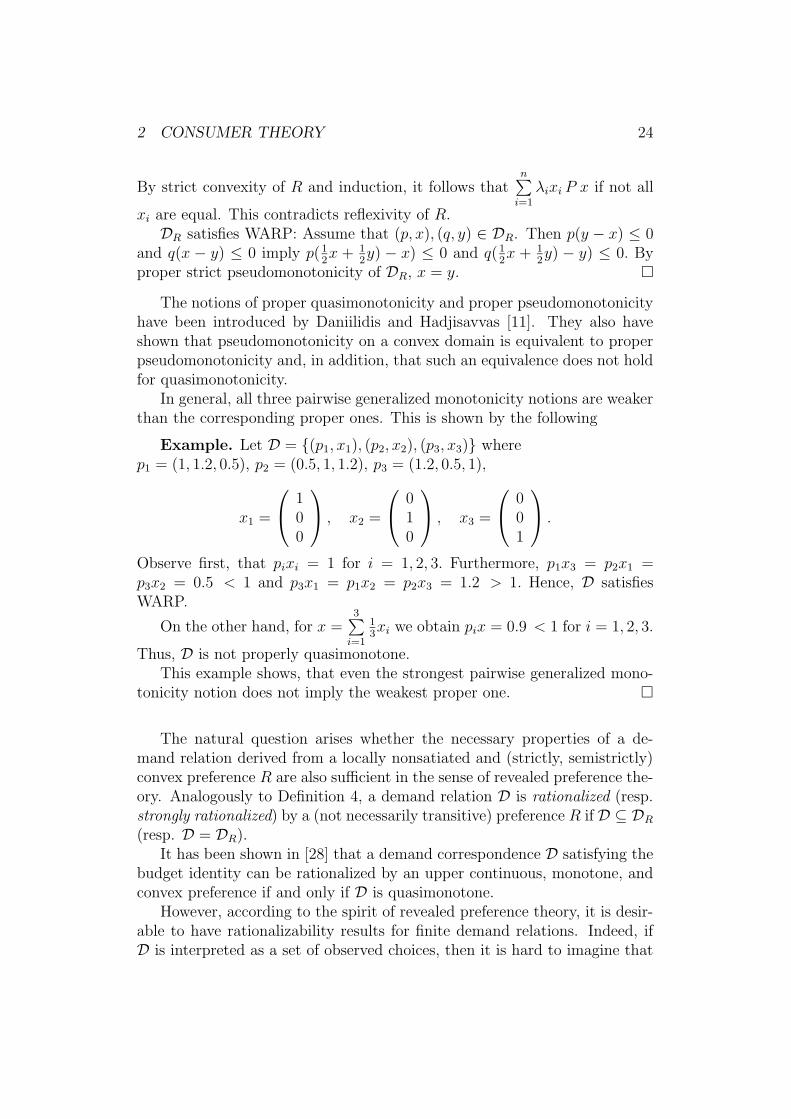
Example. Let D = {(p1, x1), (p2, x2), (p3, x3)} wherep1 = (1, 1.2, 0.5), p2 = (0.5, 1, 1.2), p3 = (1.2, 0.5, 1),

x1 =

100

, x2 =

010

, x3 =

001

.

Observe first, that pixi = 1 for i = 1, 2, 3. Furthermore, p1x3 = p2x1 =p3x2 = 0.5 < 1 and p3x1 = p1x2 = p2x3 = 1.2 > 1. Hence, D satisfiesWARP.

On the other hand, for x =3

∑

i=1

13xi we obtain pix = 0.9 < 1 for i = 1, 2, 3.

Thus, D is not properly quasimonotone.This example shows, that even the strongest pairwise generalized mono-

tonicity notion does not imply the weakest proper one. �

The natural question arises whether the necessary properties of a de-mand relation derived from a locally nonsatiated and (strictly, semistrictly)convex preference R are also sufficient in the sense of revealed preference the-ory. Analogously to Definition 4, a demand relation D is rationalized (resp.strongly rationalized) by a (not necessarily transitive) preference R if D ⊆ DR

(resp. D = DR).It has been shown in [28] that a demand correspondence D satisfying the

budget identity can be rationalized by an upper continuous, monotone, andconvex preference if and only if D is quasimonotone.

However, according to the spirit of revealed preference theory, it is desir-able to have rationalizability results for finite demand relations. Indeed, ifD is interpreted as a set of observed choices, then it is hard to imagine that


D is a demand correspondence which would require demand observations forall price vectors.

From this viewpoint, there is a result in [28] stating that an arbitrary (inparticular finite) demand relation satisfying the budget identity is properlyquasimonotone if and only if it is rationalized by a reflexive, upper continu-ous, monotone, and convex relation R.

Unfortunately, this result is not satisfactory. It does not ensure the exis-tence of rationalizing preference since R is not complete.

Put differently, it is desirable to solve the following open

Problem: Let D = {(p1, x1), ..., (pn, xn)} be a finite demand relationsuch that pixi = 1 for all i = 1, ..., n. Does there exist a locally nonsatiated,upper continuous, and convex (resp. semistrictly convex, strictly convex)preference that rationalizes D if and only if D is properly quasimonotone(resp. pseudomonotone, strictly pseudomonotone)?

At least, there is a result analogous to Proposition 7. In order to presentit, we have to introduce the generalization of the utility representation to thenontransitive case which is due to Shafer [40].

Definition 7 A real-valued function r defined on Rl+ × R

l+ is called a (nu-

merical) representation of the preference R if for all x, y ∈ Rl+ the following

conditions are satisfied:

(1) xR y ⇔ r(x, y) ≥ 0(2) r(x, y) = −r(y, x).

Notice that a utility representation u of a transitive preference � yieldsa representation in this sense by defining ru(x, y) = u(x) − u(y). It is alsoobvious that any preference R can be represented. Defining the indifferencerelation I by x I y iff xR y and y R x, completeness of R implies R

l+ × R

l+ =

P ∪ I ∪ P−1. Since R = P ∪ I, R is represented by the function r that takesthe values 1 on P , 0 on I, and −1 on P−1.

On the other hand, it is clear that any skew-symmetric function r :R

l+ × R

l+ −→ R

l+ induces a complete preference Rr which is represented

by r (define xRr y ⇔ r(x, y) ≥ 0). If R is continuous then Rr is also contin-uous. Conversely, it has been shown in [40] that every continuous preferencehas a continuous representation. Put differently, describing a ”nontransitiveconsumer” by a continuous preference is equivalent to a description by acontinuous and skew-symmetric real-valued bifunction on R

l+. Of course, the

relationship is not one-to-one since any sign-preserving transformation of arepresentation of R also represents R.


Corresponding to the possible properties of a preference R, we say thatthe representation r is nonsatiated, if for every x ∈ R

l+ there exists y ∈ R

l+

such that r(y, x) > 0 (observe that this is weaker than local nonsatiation).Since strict monotonicity means r(x, y) > 0 if x > y, we call the stronger

condition∀x, y, z ∈ R

l+ : x > y ⇒ r(x, z) > r(y, z) (30)

strong monotonicity of r.Finally, a concave utility representation is generalized by a concave-convex

representation, i.e. for every x ∈ Rl+ the function r(·, x) : R

l+ −→ R is

concave (resp. r(x, ·) is convex).Saying that r rationalizes D if Rr rationalizes D, we can state

Proposition 9 For a finite demand relationD = {(p1, x1), ..., (pn, xn)} the following conditions are equivalent:

(i) There exists a nonsatiated, concave-convex representation that ratio-nalizes D.

(ii) D is monotone transformable, i.e. there exist real numbersπi > 0 (i = 1, ..., n) such that

(πipi − πjpj)(xi − xj) ≤ 0 (31)

for all i, j ∈ {1, ..., n}.

(iii) There exists a continuous, strongly monotone, concave-convex repre-sentation that rationalizes D.

Proof See [29]. �

Notice that monotone transformability by the numbers πi means thatthe relation D = {(πipi, xi) | i = 1, ..., n} is monotone. Thus, this propertyis completely analogous to the transformability into a cyclically monotonerelation which has been observed as equivalent to GARP.

As shown in [29], monotone transformability is a generalized monotonic-ity property that is weaker than cyclic pseudomonotonicity but strongerthan proper pseudomonotonicity. Corresponding to the open problem above,proper pseudomonotone (resp. quasimonotone, strictly pseudomonotone) de-mand relations might be those which are rationalized by semistrictly quasi-concave-quasiconvex (resp. quasiconcave-quasiconvex, strictly quasiconcave-quasiconvex) representations.


We turn now to the case of continuously differentiable demand functions.Their foundation on properties of the underlying preference will not be con-sidered here. For that, we refer to [35] or, with regard to the nontransitivecase, to [3]. Instead, we shall derive some first order implications of pseu-domonotonicity that will be used in Section 3.

Let the demand relation D be represented by the continuous differentiablefunction h : R

l++ −→ R

l+, i.e.(p, x) ∈ D iff h(p) = x. As before, we assume

the budget identity ph(p) = 1 for all p.Remember that we have normalized the representation of the budget sets

by choosing wealth equal to one. Consequently, demand f(p, w) at the pricevector p and arbitrary wealth w can be derived from h by f(p, w) = h( p

w). By

definition, f is homogeneous of degree 0 in p and w and satisfies the budgetidentity pf(p, w) = w for all p and w.

Now assume that D is pseudomonotone as defined above. We claim thatthis is equivalent to the ”weak WARP ” (WWA)9 for the demand functionf , i.e.

pf(p′, w′) ≤ w implies p′f(p, w) ≥ w′ (32)

for all (p, w), (p′, w′) ∈ Rl+1++.

Indeed, by setting q = p

wand q′ = p′

w′, it follows that pf(p′, w′) ≤ w is

equivalent to q(h(q′) − h(q)) ≤ 0 and that q′(h(q′) − h(q)) ≤ 0 is equivalentto p′f(p, w) ≥ w′.

In a straightforward way, WWA implies that, for fixed wealth w, thefunction f(·, w) is pseudomonotone. By homogeneity of f , it is easy to seethat the reverse implication also holds, i.e. if f(·, w) is pseudomonotone forsome w then f satisfies WWA.

Since f(p, w) does not vanish, pseudomonotonicity of f(·, w) is equivalentto the following first order condition (see [9]):

For all p ∈ Rl++, the Jacobian matrix ∂pf(p, w) is negative semidefinite

on f(p, w)⊥, i.e. for all v ∈ Rl,

vT f(p, w) = 0 implies vT ∂pf(p, w)v ≤ 0. (33)

There is a similar first order condition that involves the Slutsky matrix off at (p, w) which is defined by

Sf(p, w) := ∂pf(p, w) + ∂wf(p, w)f(p, w)T . (34)

This matrix is derived from the income compensated demand function gat (p, w) that is defined by

g(q) = f(q, qf(p, w)). (35)

9In the economic literature, the abbreviation WWA has come into use since it wasintroduced in [30].

3 GENERAL EQUILIBRIUM THEORY 28

Indeed, by the chain rule of differentiation, it is easy to check thatSf(p, w) is equal to the Jacobian ∂g(q) evaluated at p.

The Slutsky matrix can be interpreted as a measure of substitutabilityof the commodities if prices change in such a way that real income (givenby the initially demanded bundle) stays the same. For example, if incomecompensated demand does not change there is no substitution at all, i.e. theSlutsky matrix is zero.

The first order characterizations of WWA can now be summarized in

Proposition 10 If f is continuously differentiable then the following condi-tions are equivalent:

(i) f satisfies WWA.

(ii) For some (resp. all) w > 0, the Jacobian matrices ∂pf(p, w) of thefunction f(·, w) are negative semidefinite on f(p, w)⊥.

(iii) For all p and w, the Slutsky matrix Sf(p, w) is negative semidefinite,i.e.

vT Sf(p, w)v ≤ 0 for all v ∈ Rl. (36)

Proof The equivalence of (i) and (ii) has been already mentioned beforeand was first proved by Hildenbrand and Jerison [19].

In order to prove that (ii) implies (iii), observe that any v ∈ Rl can be

written as v = u + λpT , where λ = vT f(p, w)/w such that u ⊥ f(p, w). It isnot difficult to check that the budget identity implies pSf(p, w) = 0 and thathomogeneity of f implies Sf(p, w)pT = 0. By definition of Sf(p, w), it followsthat vT Sf(p, w)v = uT Sf(p, w)u = uT ∂pf(p, w)u ≤ 0 since u ⊥ f(p, w).

Assume now (iii) and consider the Slutsky equation ∂pf(p, w) =Sf(p, w) − ∂wf(p, w)f(p, w)T . Thus, if v ⊥ f(p, w) then vT ∂pf(p, w)v =vT Sf(p, w)v ≤ 0. �

The first order characterization of WWA by the negative semidefinitenessof the Slutsky matrices is due to Kihlstrom, Mas-Colell, and Sonnenschein[30] and probably the first one obtained for a generalized monotonicity prop-erty.

3 General Equilibrium Theory

3.1 Variational Inequalities and Economic Equilibrium

Consider below the graphical illustration of a competitive equilibrium ona market for a certain commodity that is well known from all elementarytextbooks (Figure 6).


x

p

S(p)

D(p)

*p

Figure 6

It is assumed that for any given market price p there are quantities D(p)and S(p) of that commodity which describe demand and supply for the com-modity at p. An equilibrium on this market is a price p∗ for which demandequals supply, i.e. p∗ such that D(p∗) = S(p∗).

The situation depicted in Figure 6 is a nice one. There is a unique equi-librium price that is stable with respect to a price adjustment according tothe sign of excess demand: If the price increases in the case that demand ex-ceeds supply and decreases in the opposite case, then the price always adjuststowards p∗. Denoting the excess demand by

E(p) = D(p) − S(p), (37)

we obtain for every p 6= p∗ the inequality

E(p)(p∗ − p) > 0, (38)

i.e. p∗ is a solution to the Minty variational inequality problem with respectto the excess demand function E.

Of course, this is a very simple example in which a certain market isconsidered separately. In reality, there are markets for a large number ofcommodities and demand and supply on each market may depend in generalon all prices.

In order to model such an environment, we consider a comprehensivecollection of l commodities i = 1, ..., l and an excess demand function

E : P −→ Rl


defined on a convex set P of price vectors p = (p1, ..., pl) ∈ Rl. Of course,

Ei(p) is interpreted as the excess demand for commodity i at the marketprices p1, ..., pl. At the moment, we are not concerned about a derivation ofthese functions from a model of individual behaviour, i.e. they are simplytaken as given.

With regard to the domain P , it is often assumed that P ⊆ Rl+, i.e.

negative prices are excluded. However, in general this is too restrictive (seee.g. [41]).

If P = Rl++, an equilibrium is given by a price vector p∗ ∈ P such that

E(p∗) = 0, i.e. demand equals supply on each market . In the case that Eis defined on P = R

l+, the appropriate concept is a free-disposal equilibrium,

i.e. p∗ ∈ Rl+ such that E(p∗) ≤ 0 and p∗E(p∗) = 0. Such a p∗ is also known

as a solution to the nonlinear complementary problem with respect to E andallows a negative excess demand Ei(p

∗) for commodity i if the price p∗i is

equal to zero.In general, an equilibrium for the excess demand function E : P −→ R

l

is a solution to the Stampacchia variational inequality problem for E, i.e. aprice vector p∗ ∈ P such that for all p ∈ P

(p − p∗)E(p∗) ≤ 0. (39)

We remark that this definition is easily extended to the case of an excessdemand correspondence by using the same solution concept for multi-valuedmappings.

The relevance of generalized monotonicity to the theory of general eco-nomic equilibrium is demonstrated by the following results.

The first one is of course well known from the theory of variational in-equalities (see e.g. [26]).

Proposition 11 Let E : P −→ Rl be continuous.

(1) If E is pseudomonotone then p∗ ∈ P is an equilibrium for E if andonly if p∗ solves the Minty variational inequality problem with respectto E, i.e. for all p ∈ P

(p∗ − p)E(p) ≥ 0. (40)

In particular, the set of equilibria is convex.

(2) If E is strictly pseudomonotone then p∗ ∈ P is an equilibrium for Eif and only if p∗ solves the strict Minty variational inequality problemwith respect to E, i.e. for all p ∈ P such that p 6= p∗

(p∗ − p)E(p) > 0. (41)

In particular, there is at most one equilibrium .


It should be noticed that pseudomonotonicity (resp. strict pseudomono-tonicity) of E is also necessary if the set of equilibria are required to beconvex (resp. to contain at most one element) for any restriction of E to a(one-dimensional) convex subset of P (see [26]).

Proposition 11 implies the next result that was suggested in [26] andproved in [31].

Proposition 12 Let E : P −→ Rl be continuously differentiable on the open

convex domain P. If E is (strictly) pseudomonotone and p∗ is an equilibriumfor E, then

p(t) = p∗ (42)

is a (globally asymptotically) stable solution of the autonomous dynamicalsystem

p = E(p) (43)

on P.

Proof Define V (p) := (p∗ − p)2. Since V is obviously positive definite and

V (p) = ∂V (p)E(p) = −2(p∗ − p)E(p), (44)

Proposition 11 implies V (p) ≤ 0 (resp. V (p) < 0) if E is pseudomonotone(resp. strictly pseudomonotone). Thus, V is a (strict) Liapunov function forp∗ on P which proves the claim (see Theorem 1 in Chapter 9, §3 in [20]). �

The differential equation p = E(p) in Proposition 12 has a straightfor-ward economic interpretation. If p is not an equilibrium price vector thenprices adjust according to the sign of excess demand, i.e. a certain commod-ity price increases in case of excess demand and decreases in case of excesssupply for that commodity. This price adjustment is known as the Walrasiantatonnement process.

In the following sections we investigate two examples for an excess de-mand function. They will be derived from specific economic models suchthat one can ask for conditions that imply excess demand to be (strictly)pseudomonotone. For convenience, production activities are not considered.These are taken into account in a survey by Brighi and John [6].

3.2 Distribution Economies

A simple economic model that nevertheless allows to develop a nontrivialgeneral equilibrium theory had been already suggested by Cassel [7], [8] andwas later explicitly formulated by Malinvaud [33] who called it a distributioneconomy.


Its simplicity is due to the assumption that there is an exogenously givenvector y ∈ R

l++ which represents a fixed supply of l consumption goods.

These goods are demanded by a finite set H of consumers (or households)who are described by their wealth wh > 0 and by their demand function fh.

We assume that for each h ∈ H the demand function f h : Rl++×R++ −→

Rl+ is continuous and satisfies the budget identity

pfh(p, w) = w (45)

for all p and w.Given the individual characteristics (f h, wh)h∈H , the aggregate (or market)

demand function F : Rl++ −→ R

l+, defined by

F (p) =∑

h∈H

fh(p, wh) (46)

is continuous and satisfies the aggregate budget identity

pF (p) = W (47)

where W =∑

h∈H

wh denotes aggregate wealth.

The aggregate (or market) excess demand function E : Rl++ −→ R

l isthen given by E(p) = F (p) − y.

As a basic requirement, we have to ensure the existence of an equilibrium.

Proposition 13 Assume that the consumption sector (f h, wh)h∈H

satisfies the following boundary condition:For each sequence (pn)n∈N of price vectors in R

l++ that converges to some

p ∈ Rl+ \ R

l++, the sequence (fh(pn, wh))n∈N is unbounded for at least one

consumer h.Then, for any y ∈ R

l++, there exists an equilibrium of the distribution

economy E = ((fh, wh)h∈H , y).

Proof For each n ∈ N, define Sn = {p ∈ Rl++ | py = W , pi ≥

1n· W

lyi

for

i = 1, ..., l}. Since p =(

Wly1

, ..., Wlyl

)

∈ Sn, Sn is a nonempty, convex and

compact subset of Rn++.

By the fundamental existence theorem of Hartman and Stampacchia [16], foreach n ∈ N there is pn ∈ Sn such that (p − pn)E(pn) ≤ 0 for all p ∈ Sn. Inparticular,

(p − pn)E(pn) = pE(pn) = pF (pn) − W ≤ 0. (48)

This implies that the sequence (F (pn))n∈N and, consequently, all sequences(fh(pn, wh))n∈N are bounded.


Since (pn)n∈N is a sequence in the bounded set S = {p ∈ Rl++ | py =

W}, there is a subsequence (pk)k∈N converging to some p ∈ S = {p ∈R

l+ | py = W}. By the boundary condition, p 6∈ R

l+ \ R

l++, i.e. p ∈ S.

Consider an arbitrary p ∈ S. Then there is some k0 such that p ∈ Sk

for k ≥ k0. Hence, (p − pk)E(pk) ≤ 0 for k ≥ k0 and, by continuity of E,(p − p)E(p) = pE(p) ≤ 0. It follows that pE(p) ≤ 0 for all p ∈ S.Defining pi by pi

i = Wyi

and pij = 0 for i 6= j, we obtain piy = pi

iyi = W , i.e.

pi ∈ S. Thus piE(p) = Wyi

Ei(p) ≤ 0 and, consequently, Ei(p) ≤ 0. Since this

inequality holds for all i = 1, ..., l, E(p) ≤ 0. From p ∈ Rl++ and pE(p) = 0,

it follows that E(p) = 0. �

Obviously, the boundary condition in Proposition 13 that ensures theexistence of an equilibrium means that each commodity is desirable for atleast one consumer. From an economic viewpoint, such an assumption is notstrong.

We have seen that an equilibrium p∗ ∈ Rl++ is necessarily an equilibrium

with respect to the restricted excess demand function E ′ : S −→ Rl, where

S = {p ∈ Rl++ | py = W }. It turns out that E ′ is (strictly) pseudomonotone

if the corresponding property holds for the aggregate demand function F .Applying Proposition 11 yields

Proposition 14 If the aggregate demand function F is pseudomonotone,then the set of all equilibria is nonempty, compact and convex. There is aunique equilibrium if F is strictly pseudomonotone.

Proof The equilibrium set is compact as a closed subset of a bounded set.The convexity (resp. uniqueness) property follows from Proposition 11 ifwe show that (strict) pseudomonotonicity of F implies (strict) pseudomono-tonicity of E ′.

In order to prove this, consider p, q ∈ S such that p 6= q and (p−q)E(q) =(p − q)(F (q) − y) ≤ 0. Since (p − q)y = 0, it follows that (p − q)F (p) ≤ 0.If F is pseudomonotone, (p − q)F (p) ≤ 0 and, thus, (p − q)(F (p) − y) =(p − q)E(p) ≤ 0. Analogously, strict pseudomonotonicity implies that theinequalities are strict. �

What conditions ensure that aggregate demand is pseudomonotone? Ifthere were only one consumer, then this property would be implied by theWeak Axiom of Revealed Preference. However, pseudomonotonicity is notadditive. Of course, assuming monotone individual demand functions iseven sufficient for monotone aggregate demand. Since this assumption istoo strong, one has to look for another solution to the problem.


A promising approach, convincingly presented by Hildenbrand [17], is totake the distribution of the individual characteristics into account. In hisbook, he has derived various (generalized) monotonicity properties of aggre-gate demand by postulating different kinds of heterogeneous consumptionsectors.

One of these is the hypothesis of increasing dispersion of households’ de-mands. It was already studied by Jerison [23], [24] and implies that marketdemand is (strictly) pseudomonotone.

We choose to present another hypothesis in this section which even impliesmonotonicity of market demand. The reason is that pseudomonotonicityof market demand, although sufficient for a well-behaved excess demandfunction on the restricted domain S, does not yield such nice properties onR

l++.

In particular, we obtain the following negative result.

Proposition 15 Assume that F : Rl++ −→ R

l+ is not monotone at some p

with strictly positive demand F (p), i.e. (p − q)(F (p) − F (q)) > 0 for someother q. Then there is a supply vector y such that the distribution economygiven by F and y has an equilibrium which is not a solution to the Mintyvariational inequality problem with respect to the excess demand E on R

l++.

Proof If y is chosen equal to F (p) then F (p) = y, i.e. p is an equilibrium.On the other hand, (p− q)E(q) = (p− q)(F (q)− y) = −(p− q)(y −F (q)) =−(p − q)(F (p) − F (q)) < 0. �

In order to exclude the case described in the proposition above, we needa condition that guarantees monotonicity of market demand. Since we donot want to impose this property on individual demand, from which it wouldfollow trivially for aggregate demand, such a condition also provides an ex-ample that aggregation may create properties that are not satisfied at theindividual level.

In the sequel, we assume that all demand functions f h are continuouslydifferentiable. Consequently, the market demand function F is also continu-ously differentiable.

It is known that F is monotone if the Jacobian matrix ∂F (p) is negativesemidefinite for every p ∈ R

l++. Moreover, if all these matrices are negative

definite, then F is strictly monotone.By definition of aggregate demand,

∂F (p) =∑

h∈H

∂pfh(p, wh), (49)


which, by the Slutsky decomposition (see (34))

∂pfh(p, wh) = Sfh(p, wh) − ∂wfh(p, wh) fh(p, wh)

T , (50)

implies that∂F (p) = S(p) − A(p), (51)

where S(p) =∑

h∈H

Sfh(p, wh) and A(p) =∑

h∈H

∂wfh(p, wh) fh(p, wh)T .

Assuming that all consumers satisfy WWA, the individual Slutsky ma-trices Sfh(p, wh) are negative semidefinite and, thus, S(p) is also negativesemidefinite.

In order to establish the negative semidefiniteness of ∂F (p), it remains toshow that A(p) is positive semidefinite.

The matrix A(p) is positive semidefinite if and only if its symmetrizedmatrix

M(p) := A(p) + A(p)T (52)

is positive semidefinite.By the product rule of differentiation, we obtain

∂wfhi (p, wh) fh

j (p, wh) + ∂wfhj (p, wh) fh

i (p, wh) = ∂w[fhi (p, wh) fh

j (p, wh)]

or, in matrix notation,

M(p) =∑

h∈H

∂w[fh(p, wh) fh(p, wh)T ]. (53)

Let v 6= 0 be an arbitrary vector in Rl. Then

vT M(p)v =∑

h∈H

∂w[vT fh(p, wh) fh(p, wh)T v]

= ∂w

∑

h∈H

[vT fh(p, wh)]2.

Now observe that

∑

h∈H

[vT fh(p, wh)]2 = |H| · m2{vT fh(p, wh) | h ∈ H }, (54)

where m2 denotes the second moment of a set of numbers.Imagine the hypothetical situation that the wealth wh of each consumer

increases by a small amount ∆ > 0. This will lead to the demand vectors


fh(p, wh+∆), h ∈ H. Consider the set of numbers {vT fh(p, wh+∆) | h ∈ H}and define

s(p, v) := lim∆→0

1

∆[m2{vT fh(p, wh +∆) | h ∈ H}−m2{vT fh(p, wh) | h ∈ H}].

By definition, it follows immediately that

|H| · s(p, v) = ∂w

∑

h∈H

[vT fh(p, wh)]2. (55)

Consequently, s(p, v) ≥ 0 implies vT M(p)v ≥ 0 and M(p) is positive semidef-inite if s(p, v) ≥ 0 for all v.

What is the interpretation of the latter condition? The numbersvT fh(p, wh + ∆), h ∈ H, represent the orthogonal projections of the de-mand vectors fh(p, wh +∆), h ∈ H, onto the straight line through the originwith direction v. The second moment can be interpreted as a measure ofspread around zero of this set of numbers. If, for small ∆ > 0,

m2{vT fh(p, wh + ∆) | h ∈ H} ≥ m2{vT fh(p, wh) | h ∈ H}, (56)

the spread of the demand vectors fh(p, wh) is increasing in the direction v.It implies that s(p, v) ≥ 0.

Now, we say that the demand sector satisfies the hypothesis of (strictly)increasing spread around the origin, if s(p, v) ≥ 0 (resp. > 0) for everyp ∈ R

l++ and every v 6= 0, i.e. if the spread of the demand vectors f h(p, wh)

is (strictly) increasing in every direction. Thus we have proved

Proposition 16 The aggregate demand function of the consumption sectorgiven by (fh, wh)h∈H is (strictly) monotone provided that the hypothesis of(strictly) increasing spread holds.

For a detailed discussion and justification of the hypothesis of increasingspread we refer to [17].

3.3 Exchange Economies

In contrast to the concept of a distribution economy, an exchange economyis characterized by private ownership of the commodities supplied and bywealth that is dependent on prices. More precisely, the economy is given bya set H of households (or consumers) who are, for each h ∈ H, described bya demand function fh and an initial endowment eh ∈ R

l+.


For any price vector p ∈ P = Rl++, the wealth wh of consumer h is

determined by the value of his endowments at that price, i.e. wh = peh.Thus, the demand of h ∈ H at p ∈ P is given by

dh(p) := fh(p, peh). (57)

Assuming that fh is homogeneous of degree 0 in p and w, i.e. fh(λp, λw) =fh(p, w) for λ > 0, and satisfies the budget identity pf h(p, w) = w, we canconclude that dh is homogeneous of degree 0 in p, i.e. dh(λp) = dh(p) forλ > 0, and that

pdh(p) = peh. (58)

Aggregate demand is then defined by

D(p) =∑

h∈H

dh(p). (59)

Clearly, D is homogeneous of degree 0 and satisfies Walras’ Law, i.e.pD(p) = pe, where e =

∑

h∈H eh is the vector of total endowments.An equilibrium of the exchange economy is a price vector p∗ ∈ R

l++ such

thatD(p∗) = e. (60)

Equivalently, p∗ is a zero of the aggregate excess demand function Z :R

l++ −→ R

l+, defined by

Z(p) = D(p) − e. (61)

Again, Z is homogeneous of degree 0 and satisfies Walras’ Law, i.e.pZ(p) = 0 for all p.

Observe that Z can be also written as the sum of the individual excessdemand functions, i.e.

Z(p) =∑

h∈H

zh(p), (62)

where zh(p) = dh(p) − eh.By homogeneity of Z, if p∗ is an equilibrium then λp∗ is also an equi-

librium for every λ > 0. If we say that there is a unique equilibrium, itmeans uniqueness up to positive scalar multiples. Put differently, only rel-ative prices can be uniquely determined by an equilibrium of an exchangeeconomy.

In order to prove the existence of an equilibrium, prices can be nor-malized by restricting the domain P to the open unit simplex S = {p ∈R

l++ |

∑l

i=1 pi = 1}. Using this restriction, the proof of the next result isessentially analogous to the proof of Proposition 13.


Proposition 17 Assume that the individual demand functions f h are con-tinuous and satisfy the following boundary condition:

For every sequence (pn)n∈N of price vectors in Rl++ that converges to some

p ∈ Rl+ \ R

l++ and every wealth sequence (wn)n∈N that converges to some

w > 0, the sequence (fh(pn, wn))n∈N is unbounded.Then there exists an equilibrium of the exchange economy E = (f h, eh)h∈H

provided that the aggregate endowment vector is strictly positive.

Proof For each n ∈ N, define a subset Sn of S by Sn := {p ∈ S | pi ≥1nl

for i = 1, ..., l}. Since p = ( 1l, ..., 1

l) ∈ Sn for all n ∈ N, each Sn is nonempty,

convex, and compact. By continuity of Z, the existence result by Hartmanand Stampacchia [16] implies that there is, for each n ∈ N, pn ∈ Sn such that(p − pn)Z(pn) ≤ 0 for every p ∈ Sn. In particular,

(p − pn)Z(pn) = pZ(pn) =1

l

l∑

i=1

Zi(pn) ≤ 0. (63)

It follows thatl

∑

i=1

Di(pn) ≤

l∑

i=1

ei, i.e. the sequence D(pn) is bounded.

Consequently, all sequences dh(pn) = fh(pn, pneh) are bounded.The sequence (pn)n∈N in S has a subsequence (pk)k∈N that converges to

some p∗ ∈ S = cl S. Hence, for every h ∈ H, pkeh converges to p∗eh. However,p∗eh > 0 for some h ∈ H since otherwise

∑

h∈H

p∗eh = p∗∑

h∈H

eh = p∗e = 0,

contradicting e � 0.By the boundary condition, p∗ 6∈ R

l+\R

l++, i.e. p∗ ∈ S. From the definition

of the sets Sn it follows that an arbitrary p ∈ S is an element of Sk for all kgreater or equal than some k0. Hence, (p − pk)Z(pk) ≤ 0 for k ≥ k0 and, bycontinuity of Z, (p − p∗)Z(p∗) = pZ(p∗) ≤ 0.

This implies qZ(p∗) ≤ 0 for all q ∈ S = cl S, in particular for qi definedby qi

i = 1 and qij = 0 for i 6= j. Thus, Zi(p

∗) = qiZ(p∗) ≤ 0 for i = 1, ..., l.Since p∗ ∈ R

l++ and p∗Z(p∗) = 0, it follows that Z(p∗) = 0. �

Of course, existence is only a minimal requirement. It is desirable thatthere is a unique equilibrium in S which, in addition, should display somestability property, for example, to be a Minty equilibrium point with respectto Z.

Here, the situation is more difficult than in the case of a distributioneconomy. Even if one is willing to accept that all consumers have strictlymonotone demand functions (which implies a strictly monotone market de-mand), the problem is that wealth is dependent on prices and endowments.


It turns out that the distribution of endowments matters a lot.10

Consequently, one has to rely on distributional assumptions in order toobtain a uniqueness result. Such an assumption has been introduced byJerison [25] and will be presented below.

We suppose that all demand functions fh are continuously differentiableand satisfy WWA (see Section 2.3). From the Slutsky equation

∂pfh(p, w) = S fh(p, w) − ∂wfh(p, w)fh(p, w)T (64)

we obtain by the chain rule of differentiation a similar decomposition of theJacobian of individual excess demand,

∂zh(p) = ∂dh(p) = ∂pfh(p, peh)

= S fh(p, peh) − ∂wfh(p, peh)zh(p)T . (65)

Now imagine that, hypothetically, the nominal wealth peh increases by∆ ≥ 0 for each h ∈ H and denote by

zh(p, ∆) = fh(p, peh + ∆) − eh (66)

the excess demand of consumer h after this increase. The mean excess de-mand of the wealthier population is then given by

Z(p, ∆) =1

|H|

∑

h∈H

zh(p, ∆). (67)

Let v 6= 0 be an arbitrary vector in Rl. The dispersion of excess demand

at (p, ∆) in the direction v is defined as the variance of the real variablevT zh(p, ∆), i.e.

σ2v(p, ∆) =

1

|H|

∑

h∈H

[vT zh(p, ∆) − vT Z(p, ∆)]2. (68)

Clearly, for ∆ = 0, σ2v(p, 0) denotes the dispersion of excess demand for the

actual situation.

Definition 8 The exchange economy satisfies the hypothesis of increasingdispersion of excess demands (IDED), if for all p ∈ R

l++ and all v 6= 0 such

that pv = vT Z(p) = 0, ∂∆σ2v(p, 0) > 0.

10The standard example where uniqueness is likely to fail is an economy with two com-modities and two consumers such that each consumer owns only one of these commoditiesand has also a relatively high propensity to consume the same commodity.


Notice that IDED does not imply particular restrictions on the distribu-tion of the demand functions fh or the distribution of endowments eh. It isa hypothesis on the joint distribution of individual characteristics (f h, eh).Let us illustrate this point by a simple example with two goods and twoconsumers.

Example. The utility functions of the agents a and b are respectivelyua(x, y) = min{x, 2y} and ub(x, y) = min{2x, y}. Accordingly, their de-mands are given by

fa(p, w) =

(

2w

2p1 + p2

,w

2p1 + p2

)

, f b(p, w) =

(

w

p1 + 2p2

,2w

p1 + 2p2

)

.

(1) We shall consider first the case where the vectors of initial endowmentsare ea = (10, 0) and eb = (0, 10). If Z(p) 6= 0 the hypothesis is triviallysatisfied in the two goods case. Therefore, let us focus on the price vectorsat which Z vanishes, i.e. p = (1, 1) in the present example. This case isdepicted in Fig. 7a where the dashed line represents the budget line of eachagent after a generalized increase in income by the amount ∆ > 0. Ea andEb are the Engel curves of the two agents.

aE

bE

∆d (p, )b

d (p)b

d (p)a ∆d (p, )

a

ea

eb

p

v

Figure 7a

Fig. 7b translates the above example in terms of excess demand andclearly shows that IDED is violated.


z (p)

z (p, )∆

z (p) p

∆z (p, )

a

a

b

b

Figure 7b

(2) Now consider the case where the vectors of initial endowments are re-versed, i.e. ea = (0, 10) and eb = (10, 0). The marginal distributions of e andf are the same as before, but the joint distribution is different. This case isshown in Fig. 8a.

aE

bE

∆d (p, )b

d (p)a ∆d (p, )

a

d (p)b

eb

ea

p

v

Figure 8a

Fig. 8b shows that the dispersion of excess demand is increasing so thatIDED holds. We notice that the individual characteristics are the same asin (1), except for their joint distribution. (1) and (2) thus show that IDEDdoes not depend on the particular shape of the Engel curves.


z (p)

z (p, )∆

z (p)

z (p, )∆

p

a

a

b

b

Figure 8b

The following result which is due to Jerison [25] shows that IDED impliesa well-behaved aggregate demand of an exchange economy.

Proposition 18 Assume that the exchange economy given by(fh, eh)h∈H satisfies, in addition to assumptions which ensure existence ofan equilibrium, the hypothesis IDED.

Then, there is (up to positive scalar multiples) a unique equilibrium p∗.Moreover, the aggregate excess demand function satisfies Wald’s Axiom, i.e.for all p, q ∈ R

l++ such that Z(p) 6= Z(q),

qZ(p) ≤ 0 implies pZ(q) > 0, (69)

in particular, p∗Z(q) > 0 for every price vector q which is not an equilibrium.

Proof Our first aim is to prove that ∂Z(p) is negative definite on thesubspace of R

l that is orthogonal to p and Z(p), i.e. vT ∂Z(p)v < 0 for allv 6= 0 such that pv = vT Z(p) = 0.

From the Slutsky decomposition of the individual excess demands (65) itfollows that

∂Z(p) =∑

h∈H

Sfh(p, peh) −∑

h∈H

mh(p)zh(p)T , (70)

where we have used the abbreviation mh(p) = ∂wfh(p, peh).Since we have assumed that the individual demand functions satisfy

WWA, the sum of negative semidefinite matrices Sf h(p, peh) is negative


semidefinite. It remains to show that the matrix

A(p) =∑

h∈H

mh(p)zh(p)T (71)

is positive definite on p⊥ ∩ Z(p)⊥ or, equivalently, that A(p) = 1|H|

A(p) hasthis property.

In order to prove this, observe first that

σ2v(p, ∆) =

1

|H|

∑

h∈H

(vT [zh(p, ∆ − Z(p, ∆)])2

=1

|H|

∑

h∈H

vT [zh(p, ∆) − Z(p, ∆)] [zh(p, ∆) − Z(p, ∆)]T v

= vT

{

1

|H|

∑

h∈H

[zh(p, ∆) − Z(p, ∆)] [zh(p, ∆) − Z(p, ∆)]T

}

v

= vT cov zh(p, ∆)v,

where cov zh(p, ∆) denotes the covariance matrix of the individual excessdemands zh(p, ∆). This implies

∂∆σ2v(p, 0) = vT [∂∆ cov zh(p, 0)]v

= vT ∂∆

{

1

|H|

∑

h∈H

[zh(p, 0) − Z(p, 0)] [zh(p, 0) − Z(p, 0)]T

}

v

= vT

{

∂∆

[

1

|H|

∑

h∈H

zh(p, 0)zh(p, 0)T

]

− ∂∆[Z(p, 0)Z(p, 0)T ]

}

v

= vT

{

1

|H|

∑

h∈H

mh(p)zh(p)T +1

|H|

∑

h∈H

zh(p)mh(p)T − M(p)Z(p)T

− Z(p)M(p)T

}

v,

where M(p) = 1|H|

∑

h∈H

mh(p).

Since the last term is equal to

2vT

[

1

|H|

∑

h∈H

mh(p)zh(p)T

]

v − 2vT Z(p)M(p)T v, (72)

it follows from the assumption vT Z(p) = 0 that

∂∆σ2v(p, 0) = 2vT A(p)v. (73)


By IDED, ∂∆σ2v(p, 0) > 0. Hence, A(p) is positive definite on p⊥ ∩ Z(p)⊥

and thus we have proved that ∂Z(p) is negative definite on p⊥ ∩ Z(p)⊥.It was shown by Kihlstrom, Mas-Colell, and Sonnenschein [30] (Theorem

4) that this implies Wald’s Axiom for Z, i.e. Z(p) 6= Z(q) and qZ(p) ≤ 0implies pZ(q) > 0.

In particular, it follows by Walras’ Law that Z is pseudomonotone, i.e.

(q − p)Z(p) ≤ 0 implies (q − p)Z(q) ≤ 0 (74)

for all p, q ∈ Rl++.

Hence, the set of equilibrium prices is convex by Proposition 11. It re-mains to prove uniqueness.

Assume that p and q are two different equilibria. Setting v = q − p, weobtain Z(p + λv) = 0 for all λ ∈ [0, 1] since the equilibrium set is convex.This implies

∂λZ(p + λv) |λ=0 = ∂Z(p)v = 0. (75)

For Z(p) = 0, ∂Z(p) is negative definite on p⊥, i.e. rank ∂Z(p) = l − 1.By homogeneity of Z, ∂Z(p)pT = 0. Thus, p is collinear with v, resp. p iscollinear with q. �

Observe that the conclusions of Proposition 18 only need that ∂Z(p) isnegative definite on p⊥ ∩ Z(p)⊥. This has been shown by using the decom-position

∂Z(p) = S(p) − A(p) (76)

and by proving that IDED implies the positive definiteness of A(p) on thatsubspace (knowing that S(p) is negative semidefinite).

Alternatively, one can assume that S(p) is even negative definite on p⊥

(it cannot be negative definite on the whole space since, by homogeneity,S(p)p> = 0) and weaken IDED by the hypothesis of nondecreasing dispersionof excess demands (NDED) (see [25]), i.e. ∂∆σ2

v(p, 0) ≥ 0 for all p and v suchthat pv = vT Z(p) = 0.

The stronger assumption on S(p) can be easily justified. It means thatthere is always substitution between two commodities in case of a relativeprice change. Although it may be restrictive condition for an individual, itis an acceptable assumption for aggregate demand.

REFERENCES 45

References

[1] Afriat, S.N., The construction of utility functions from expenditure data,Int. Economic Rev. 8, 1967, 67-77.

[2] Allen, R.G.D., The foundations of a mathematical theory of exchange,Economica 12, 1932, 197-226.

[3] Al-Najjar, N., Non-transitive smooth preferences, Journal of EconomicTheory 60, 1993, 14-41.

[4] Avriel, M., Diewert, W. E., Schaible, S. and I. Zang, Generalized Con-cavity, Plenum Press, New York 1988.

[5] Berge, C., Topological spaces, Dover Publications, New York 1997.

[6] Brighi, L. and R. John, Characterizations of pseudomonotone maps andeconomic equilibrium, J. Statistics and Management Systems 5, 2002,253-273.

[7] Cassel, G., Grundriss einer elementaren Preislehre, Zeitschrift f. d. ges,Staatswissenschaft 55, 1899, 395-458.

[8] Cassel, G., Theoretische Sozialokonomie, Winter, Leipzig 1918.

[9] Crouzeix, J. P., Characterizations of generalized convexity and gener-alized monotonicity, a survey, in Generalized Convexity, GeneralizedMonotonicity, J.-P. Crouzeix, J.-E. Martinez-Legaz and M. Volle, eds.,Kluwer Academic Publishers, Dordrecht 1998, 237-256.

[10] Dafermos, S., Exchange price equilibria and variational inequalities,Math. Program. 46, 1990, 391-402.

[11] Daniilidis, A. and N. Hadjisavvas, On the subdifferentials of quasicon-vex and pseudoconvex functions and cyclic monotonicity, J. of Math.Analysis and Appl. 237, 1999, 30-42.

[12] Debreu, G., Theory of value, Wiley, New York 1959.

[13] Georgescu-Roegen, N., The pure theory of consumer’s behavior, Quar-terly J. of Economics 50, 1936, 545-593.

[14] Georgescu-Roegen, N., Choice and revealed preference, Southern Eco-nomic Journal 21, 1954, 119-130.

REFERENCES 46

[15] Harker, P.T. and J.-S. Pang, Finite-dimensional variational inequalityand nonlinear complementary problems: A survey of theory, algorithmsand applications, Math. Program. 48, 1990, 161-220.

[16] Hartman, P. and G. Stampacchia, On some nonlinear elliptic differentialfunctional equations, Acta Mathematica 115, 1966, 153-188.

[17] Hildenbrand, W., Market demand: Theory and empirical evidence,Princeton University Press, Princeton 1994.

[18] Hildenbrand, W., An exposition of Wald’s existence proof, in KarlMenger: Ergebnisse eines mathematischen Kolloquiums, E. Dierker andK. Sigmund, eds., Springer-Verlag, Wien 1998.

[19] Hildenbrand, W. and M. Jerison, The demand theory of the weak axiomsof revealed preference, Economics Letters 29, 1989, 209-213.

[20] Hirsch, M. W. and S. Smale, Differential Equations, Dynamical Systems,and Linear Algebra, Academic Press, New York 1974.

[21] Houthakker, H. S., Revealed preference and the utility function, Eco-nomica 17, 1950, 159-174.

[22] Hurwicz, L. and M. K. Richter, Revealed preference without demand con-tinuity assumptions, in Preferences, Utility, and Demand, J. S. Chipman,L. Hurwicz, M. K. Richter and H. F. Sonnenschein, eds., Harcourt BraceJovanovich, New York 1971.

[23] Jerison, M. The representative consumer and the weak axiom when thedistribution of income is fixed, Report DP 150, SUNY, Albany 1982.

[24] Jerison, M., Aggregation and pairwise aggregation of demand when thedistribution of income is fixed., J. Economic Theory 33, 1984, 1-31.

[25] Jerison, M., Dispersed excess demands, the weak axiom and uniquenessof equilibrium, J. Math. Economics 31, 1999, 15-48.

[26] John, R., Variational inequalities and pseudomonotone functions: Somecharacterizations, in Generalized Convexity, Generalized Monotonicity,J.-P. Crouzeix, J.-E. Martinez-Legaz and M. Volle, eds., Kluwer Aca-demic Publishers, Dordrecht 1998, 291-301.

[27] John, R., Abraham Wald’s equilibrium existence proof reconsidered, Eco-nomic Theory 13, 1999, 417-428.

REFERENCES 47

[28] John, R., Quasimonotone individual demand, Optimization 47, 2000,201-209.

[29] John, R., The concave nontransitive consumer, J. Global Optimization20, 2001, 297-308.

[30] Kihlstrom, R., Mas-Colell, A. and H. Sonnenschein, The demand theoryof the weak axiom of revealed preference, Econometrica 44, 1976, 971-978.

[31] Komlosi, S., On the Stampacchia and Minty variational inequalities, inGeneralized Convexity and Optimization for Economic and FinancialDecisions, G. Giorgi and F. A. Rossi, eds. Pitagora Editrice, Bologna1999.

[32] Kuhn, H. W., On a theorem of Wald, in Linear inequalities and relatedsystems, H. W. Kuhn and A. W. Tucker, eds., Annals of MathematicalStudies No. 38, Princeton University Press, Princeton 1956.

[33] Malinvaud, E. Lectures on microeconomic theory, North-Holland, Ams-terdam 1972.

[34] Mas-Colell, A., On revealed preference analysis, Rev. Economic Studies45, 1978, 121-131.

[35] Mas-Colell, A., The theory of general economic equilibrium: A differen-tiable approach, Cambridge University Press, Cambridge 1985.

[36] Mas-Colell, A., Whinston, M. D. and J. R. Green, Microeconomic theory,Oxford University Press, New York 1995.

[37] Matzkin, R. L. and M. K. Richter, Testing strictly concave rationality,J. Economic Theory 53, 1991, 287-303.

[38] Samuelson, P. A., A note on the pure theory of consumer behaviour,Economica 5, 1938, 61-72.

[39] Schlesinger, K., Uber die Produktionsgleichungen der okonomischenWertlehre, Ergebnisse eines mathematischen Kolloquiums 6, 1935, 10-11.

[40] Shafer, W. J., The nontransitive consumer, Econometrica 42, 1974, 913-919.

REFERENCES 48

[41] Shafer, W. J., Equilibrium in economies without ordered preferences orfree disposal, J. Math. Economics 3, 1976, 135-137.

[42] Shafer, W. J., Transitivity, in The New Palgrave: A Dictionary of Eco-nomics, J. Eatwell, M. Milgate and P. Newman, eds. Macmillan Press,London 1987.

[43] Sonnenschein, H. F., Demand theory without transitive preferences, withapplications to the theory of competitive equilibrium, in Preferences, Util-ity, and Demand, J. S. Chipman, L. Hurwicz, M. K. Richter and H. F.Sonnenschein, eds., Harcourt Brace Jovanovich, New York 1971.

[44] Varian, H. R., The nonparametric approach to demand analysis, Econo-metrica 50, 1982, 945-973.

[45] Wald, A., Uber die Produktionsgleichungen der okonomischen Wertlehre,Ergebnisse eines mathematischen Kolloquiums 7, 1936, 1-6.

[46] Zeuthen, F., Das Prinzip der Knappheit, technische Kombination undokonomische Qualitat, Zeitschrift f. Nationalokonomie 4, 1933, 1-24.

uses of generalized convexity and generalized monotonicity in economics

Documents