1

Using a Data Grid to Automate Data Preparation Pipelines 1

Required for Regional-Scale Hydrologic Modeling 2

Mirza M. Billah1, Jonathan L. Goodall2, 3, *, Ujjwal Narayan4, Bakinam T. Essawy2, 3

Venkat Lakshmi5, Arcot Rajasekar6, Reagan W. Moore6

4

5

1 Department of Biological Systems Engineering, Virginia Tech, Blacksburg, Virginia 6

2 Department of Civil and Environmental Engineering, University of Virginia, 7

Charlottesville, Virginia 8

3 Department of Civil and Environmental Engineering, University of South Carolina, 9

Columbia, SC 10

4 CMNS-Earth System Science Interdisciplinary Center, University of Maryland, College 11

Park, MD 12

5 Department of Earth and Ocean Sciences, University of South Carolina, Columbia, SC 13

6 School of Information and Library Science, University of North Carolina, Chapel Hill, 14

NC 15

* To whom correspondence should be addressed (E-mail: goodall@virginia.edu; 16

Address: University of Virginia, Department of Civil and Environmental Engineering, 17

PO Box 400742, Charlottesville, Virginia 22904; Tel: (434) 243-5019) 18

2

Abstract 1

Modeling a regional-scale hydrologic system introduces major data challenges 2

related to the access and transformation of heterogeneous datasets into the information 3

needed to execute a hydrologic model. These data preparation activities are difficult to 4

automate, making the reproducibility and extensibility of model simulations conducted 5

by others difficult or even impossible. This study addresses this challenge by 6

demonstrating how the integrated Rule Oriented Data Management System (iRODS) can 7

be used to support data processing pipelines needed when using data-intensive models to 8

simulate regional-scale hydrologic systems. Focusing on the Variable Infiltration 9

Capacity (VIC) model as a case study, data preparation steps are sequenced using rules 10

within iRODS. VIC and iRODS are applied to study hydrologic conditions in the 11

Carolinas, USA during the period 1998-2007 to better understand impacts of drought 12

within the region. The application demonstrates how iRODS can support hydrologic 13

modelers to create more reproducible and extensible model-based analyses. 14

15

Keywords: data management; workflows; hydrologic modeling, iRODS 16

17

Software availability: The software is provided open source and freely available on 18

GitHub. Visit https://github.com/uva-hydroinformatics-lab/VIC_Pre-Processing_Rules 19

for additional details. 20

3

INTRODUCTION 1

Motivation 2

Application of regional-scale hydrologic models presents a number of challenges 3

associated with handling and processing large datasets. These models are data intensive 4

and require a significant amount of time, effort, and resources in order to transform 5

available datasets into the form required by the model (Leonard and Duffy, 2013). The 6

information required by models is contained within multiple datasets maintained by 7

various data providers with each dataset having unique data access protocols, file 8

formats, and semantics (Horsburgh et al., 2014). The result is that the input datasets for a 9

hydrologic model require specific transformations before they can be used to setup, 10

calibrate, and validate the model (Leonard and Duffy, 2014). 11

Due to the level of heterogeneity across data sources and the inconsistent input 12

file formats required by various models, these data transformation steps are difficult to 13

automate. With the exception of a few models with robust data preparation tools, data 14

transformation steps associated with hydrologic model data preparation often require 15

significant manual intervention. Even for models with data preparation tools available, 16

these tools are often tightly coupled to pre-specified data sources that may not be the best 17

available information for a specific region or modeling objective. The end result is that 18

modelers (i) consume significant time on tasks that could be automated, (ii) lack the 19

ability to easily reproduce and extend past work completed by others, and (iii) are unable 20

to take full advantage of the most recently available information when creating models. 21

Within the information and computer science communities, there has been work 22

to create advanced data management and scientific workflow software (Foster, 2011; Gil 23

4

et al., 2007; Ludäscher et al., 2006; Moore and Rajasekar, 2014; Oinn et al., 2006). These 1

tools have been applied within many scientific communities including hydrology (Fitch 2

et al., 2011; Guru et al., 2009; Perraud et al., 2010; Piasecki and Lu, 2010). Scientific 3

workflow environments offer many benefits for implementing data preparation tasks. For 4

example, workflow environments coordinate and automate processing steps, as well as 5

track the provenance of the datasets generated through the processing steps. This is 6

important especially for reproducibility, transparency, and reuse of computational 7

analyses. 8

There remain challenges, however, in applying workflow tools for hydrologic 9

modeling support. One challenge is the lack of a common data model within hydrology 10

(Perraud et al., 2010). It is typical for hydrologic models to require gridded data in 11

NetCDF or GRIB formats, times series in CSV or WaterML format, and GIS layers in 12

shapefile, geodatabase, or raster formats. These data come from NASA, NOAA, USGS, 13

and others, with each agency adopting its own semantics and structure. Another challenge 14

is the large number of models used in the hydrology community, each with its own data 15

formats, structures, and semantics. There is significant heterogeneity across these 16

hydrologic models with some models adopting a gridded data structure and others 17

adopting a feature-oriented (e.g., watersheds and stream networks) data structure. In 18

short, there is very little commonality between input file structures and semantics across 19

hydrologic data and models. 20

For these reasons, we argue that data preparation for regional-scale hydrologic 21

modeling is a data-centric rather than process-centric task. That is to say, due to the lack 22

of a common data model in hydrology, the primary goal is to create data processing 23

5

pipelines that define the logic for integrating and transforming the information contained 1

within multiple datasets into a new product required by the hydrologic model as input. 2

While others have argued for a centralized and standardized data model for hydrology 3

(Goodall and Maidment, 2009; Leonard and Duffy, 2014; Maidment, 2002), we argue 4

here that the current level of heterogeneity in source data and model input requirements 5

makes this level of standardization, while an important long-term goal, difficult to obtain 6

in the short-term. Rather, data can remain decentralized and under the control of data 7

providers, but there should be a means for applying server-side data transformation 8

pipelines to reference datasets. These pipelines, which could be written and maintained 9

by model developers and users, will allow for on-demand access to derived data products 10

required by specific hydrologic models. In the spirit of Relational Database Management 11

Systems (RDMS), these pipelines can be thought of as views of the underlying data, 12

tailored for a specific model. 13

In this paper, we present a method for creating server-side data pre-processing 14

pipelines using the DataNet Federation Consortium (DFC) data grid, which is powered 15

by the Integrated Rule-Oriented Data System (iRODS). We illustrate the methodology 16

using the Variable Infiltration Capacity (VIC) regional-scale hydrologic model. These 17

systems are briefly introduced in the following background section. Then, in the design 18

and implementation section, the approach for automating VIC data preparation pipelines 19

using iRODS is presented. Finally, the pipelines are demonstrated for an example of 20

modeling drought in the Carolinas region of the United States. 21

6

Background 1

The DFC grid (http://www.datafed.org) was built as part of an NSF-funded 2

research project to provide storage and compute resources that allow for long-term access 3

to the stored datasets. DFC is enabled by iRODS, an open source, policy-based 4

cyberinfrastructure developed by the Data Intensive Cyber Environments (DICE) group 5

for distributed data management (Rajasekar et al., 2010b) (http://www.irods.org). It is 6

used by a wide variety of end users including various scientific communities (Chiang et 7

al., 2011; Goff et al., 2011; NASA, 2015). Data management tasks and policies are 8

implemented within iRODS as rules. Rules specify a sequence of lower-level micro-9

services that operate on datasets within the data grid. Users can specify sequences of data 10

collection, transformation, curation, preservation, and processing steps within one or 11

more rules. iRODS includes a Rule Engine (RE) that allows for remote execution of rules 12

on iRODS resource servers, which is especially beneficial for large-datasets. iRODS, 13

therefore, provides a means for uploading processing routines to data resource servers, 14

whereas the typical approach used now in hydrology is to download data for local 15

processing. 16

The Variable Infiltration Capacity (VIC) model is a large-scale hydrologic model 17

that applies water and energy balances to simulate terrestrial hydrology at a regional 18

spatial scale (Liang et al., 1996a). The scientific background of the model is summarized 19

in the case study section, while here the model is presented from a data management 20

perspective. The model requires several input datasets, and these datasets must be 21

generated through a sequence of data processing steps. Figure 1 shows the data 22

processing pipeline that is typically done manually to create the meteorological and land 23

7

surface variable inputs for a VIC model simulation. The figure illustrates the difficulties 1

in performing this workflow, which include the fact that different datasets are required, 2

each with a different data model, and processing steps are written in different languages 3

and sometimes require legacy compilers due to the time that they were developed. 4

Executing these data processing scripts currently requires significant effort, especially for 5

new users that must learn the steps and configure often complicated legacy software to 6

correctly execute the sequence of steps. While Figure 1 depicts the process as an 7

integrated workflow, in practice it is instead a sequence of steps often performed 8

independently with software developed at different times by different scientists. While 9

this description is for VIC, we believe it describes a general problem faced by other data 10

intensive models. 11

12

8

1

Figure 1: Data pre-processing steps for VIC model depicted as a flow chart of legacy 2

processing scripts written in different languages, operating on different input datasets, 3

and creating different output datasets. 4

9

Study Objective and Scope 1

Given these data challenges in running data-intensive hydrologic models, and 2

given the potential advantages of advanced data management systems such as iRODS, 3

the objective of this study is to apply iRODS to support hydrologic modeling. More 4

specifically, the focus of this research is on the data preparation pipeline used to create 5

the input files required for running VIC. The goal is to automate these steps as iRODS 6

rules. The rules provide a means for server-side execution of data processing pipelines, 7

moving closer to the long-term goal of reproducible end-to-end model simulations. The 8

study is built on prior work where the VIC model was used for simulating a period of 9

drought in South Carolina, USA (Billah and Goodall, 2011; Billah et al., 2015). VIC is a 10

widely used model for investigating regional-scale hydrologic systems (Abdulla et al., 11

1996; Lakshmi et al., 2004; Lohmann et al., 1998; Sheffield and Wood, 2007; Sheffield 12

et al., 2004), and the software resulting from the prototyping work can be used by this 13

community. More generally, the outcome of this work is a methodology for creating 14

server-side data processing pipelines that could be applied for other data-intensive 15

hydrologic, environmental, and Earth system models. 16

SYSTEM DESIGN AND IMPLEMENTATION 17

The DFC-Hydrology Grid 18

The server-side data processing software shown in Figure 1 is deployed on an 19

iRODS resource server that is part of the DFC-hydrology grid. The DFC-hydrology grid 20

is part of the larger DFC grid (Figure 2), which is funded by the National Science 21

Foundation (NSF) to support data collection, analysis, preservation, sharing, and 22

10

publication of scientific data and models (http://www.datafed.org). The DFC-hydrology 1

grid consists of an iRODS resource server that communicates with an iRODS metadata 2

catalog (iCAT) server located in the DFC grid. The iCAT server is administered by 3

RENCI (Renaissance Computing Institute) in Chapel Hill, North Carolina. iRODS also 4

includes a Rule Engine (RE) that interprets rules executed on the server, but initiated 5

from a client program. The RE connects to the catalog server in the DFC grid and updates 6

the iCAT database if new files are generated through the execution of a rule. 7

An iRODS client application is used to initiate data management tasks including 8

rules within the federated grid. A commonly used iRODS client application is the i-9

commands utility that consists of several command-line utilities for managing datasets 10

and executing data processing commands (Rajasekar et al., 2010a). These i-commands 11

can be used to put and get data into/from the DFC grids, as well as execute a set of other 12

commands for data management, analysis, and sharing. A user has the opportunity to 13

create and execute rules to chain commands for tasks such as gaining access to 14

heterogeneous data sources and processing datasets into the formats required by models 15

or scientific communities. 16

The hydrology related data collected from various external sources are stored and 17

preserved in the DFC-hydrology grid in their native formats. This data gathering process 18

can be automated using iRODS functionality and different servers within the grid. For 19

instance, the precipitation data collection can be obtained from remote servers by one 20

iRODS resource server and data transformations could be performed by a second iRODS 21

resource server in the DFC-hydrology grid. Because these servers are part of the same 22

data grid, the distributed data stored across the servers appears to client applications as 23

11

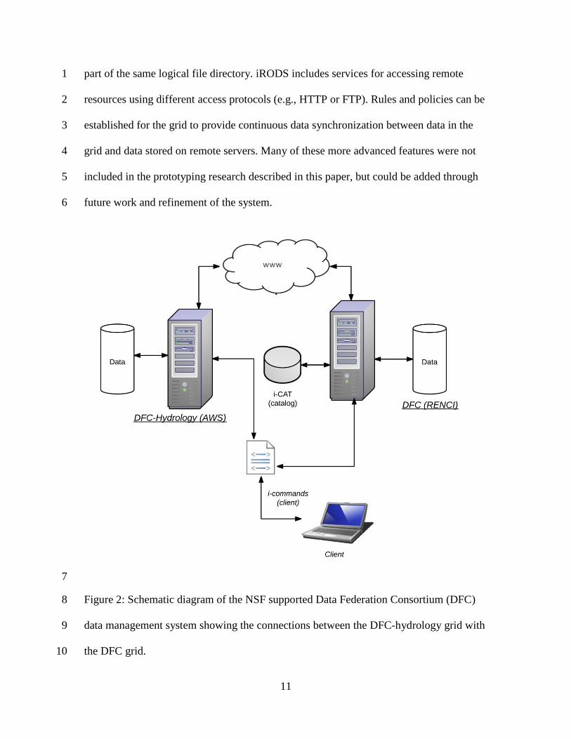
part of the same logical file directory. iRODS includes services for accessing remote 1

resources using different access protocols (e.g., HTTP or FTP). Rules and policies can be 2

established for the grid to provide continuous data synchronization between data in the 3

grid and data stored on remote servers. Many of these more advanced features were not 4

included in the prototyping research described in this paper, but could be added through 5

future work and refinement of the system. 6

7

Figure 2: Schematic diagram of the NSF supported Data Federation Consortium (DFC) 8

data management system showing the connections between the DFC-hydrology grid with 9

the DFC grid. 10

12

Micro-Services 1

Micro-services are the building blocks for implementing policy-based data 2

management within the DFC grid (Rajasekar et al., 2010a). A micro-service is a well-3

defined function that performs a specific task as part of a distributed workflow system. A 4

number of micro-services are available to automate data collection, processing, and 5

storage in the DFC federated resource servers. These micro-services are primarily 6

developed by system or application programmers, but could also be written by scientists. 7

The micro-services that are applied for this study are listed in Table 1. These micro-8

services are included in the latest iRODS release and can be chained together using rules. 9

Although the flexibility to chain a number of micro-services provides multiple ways to 10

complete a series of tasks, iRODS applies priorities and validation conditions to select the 11

best micro-service to complete a given task. 12

Table 1: Micro-services applied for VIC model application using iRODS. 13

No. Micro-service Purpose

1 msiExecCmd Execute commands

2 msiCollCreate Make data collection

3 msiDataObjCreate Create data object

4 msiDataObjWrite Write data object

5 msiDataObjClose Close data object

6 msiAddSelectFieldToGenQuery Make query for data using field

7 msiAddConditionToGenQuery Make query for data using condition

8 msiExecGenQuery Execute Query

9 msiGetValByKey Extract value from query result

10 msiSplitPath Get directory path

11 msiDataObjUnlink Delete temporary file

12 msiRmColl Remove data collection

13 msiGetSystemTime Get time stamp

14

13

Rules 1

The rule is a critical and fundamental component for iRODS. It provides a 2

flexible mechanism to integrate external systems for specialized processing and metadata 3

management (Hedges et al., 2009, 2007). In this system, we use rules to implement data 4

processing pipelines on the DFC grid. Data pre-processing rules involve collecting and 5

transforming datasets from heterogeneous sources into the inputs required by VIC. For 6

our purposes, data were collected from the United States Geological Survey (USGS), 7

National Climatic Data Center (NCDC), National Center For Atmospheric Research 8

(NCAR), National Centers for Environmental Prediction (NCEP), and Land Data 9

Assimilation System (LDAS). The DFC catalog is updated automatically when data are 10

put into the grid. This catalog functions as an information center and enables the 11

discovery of distributed data stored within the grid. 12

Data processing workflows can be implemented as rules that transform the 13

collected datasets from the external sources into model readable inputs (Figure 3). These 14

rules are a combination of multiple step-based routines, each of which performs a 15

particular task. The steps are shown in Figure 3 and include tasks such as retrieving data, 16

preparing data for gridding, adjusting observation times, and transforming gridded and 17

rescaled datasets. For our study, the routines for executing these steps are installed on a 18

resource server that is part of the DFC-hydrology grid and integrated into data-specific 19

rules used to complete a series of tasks from collection and transformation of the datasets 20

into model inputs. Separate rules were created to perform the data transformation tasks 21

grouped into logical divisions as shown in Table 2. 22

14

1

Figure 3: Model pre-processing workflows showing the major steps for transforming 2

datasets to set up the VIC model for a specific study area. Rules are initiated from a client 3

but executed on a server using micro-services. 4

15

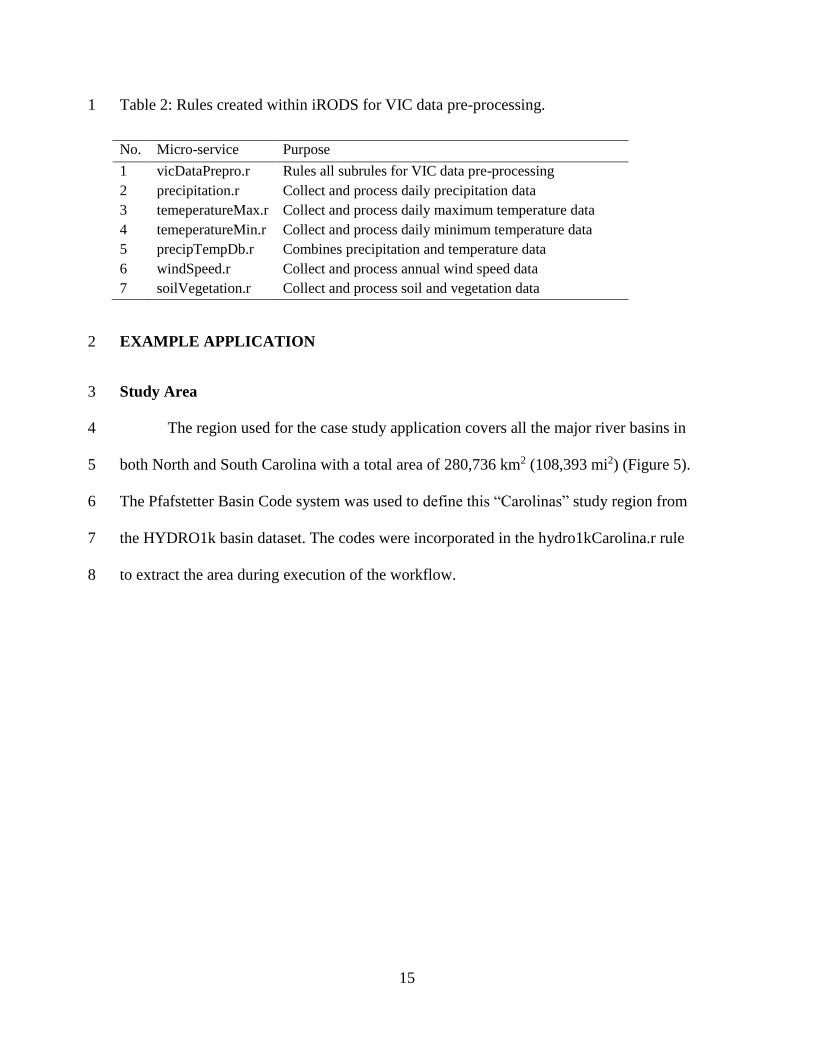
Table 2: Rules created within iRODS for VIC data pre-processing. 1

No. Micro-service Purpose

1 vicDataPrepro.r Rules all subrules for VIC data pre-processing

2 precipitation.r Collect and process daily precipitation data

3 temeperatureMax.r Collect and process daily maximum temperature data

4 temeperatureMin.r Collect and process daily minimum temperature data

5 precipTempDb.r Combines precipitation and temperature data

6 windSpeed.r Collect and process annual wind speed data

7 soilVegetation.r Collect and process soil and vegetation data

EXAMPLE APPLICATION 2

Study Area 3

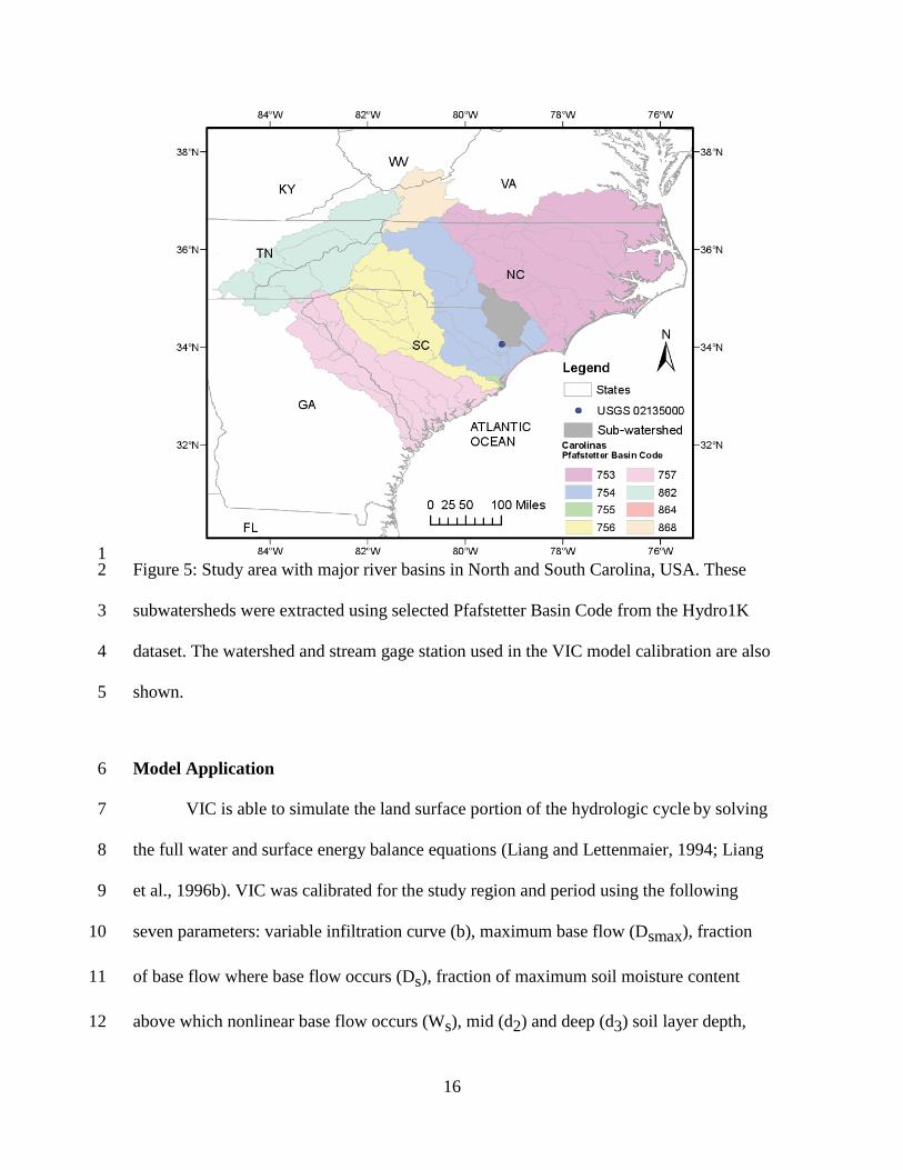
The region used for the case study application covers all the major river basins in 4

both North and South Carolina with a total area of 280,736 km2 (108,393 mi2) (Figure 5). 5

The Pfafstetter Basin Code system was used to define this “Carolinas” study region from 6

the HYDRO1k basin dataset. The codes were incorporated in the hydro1kCarolina.r rule 7

to extract the area during execution of the workflow. 8

16

1 Figure 5: Study area with major river basins in North and South Carolina, USA. These 2

subwatersheds were extracted using selected Pfafstetter Basin Code from the Hydro1K 3

dataset. The watershed and stream gage station used in the VIC model calibration are also 4

shown. 5

Model Application 6

VIC is able to simulate the land surface portion of the hydrologic cycle by solving 7

the full water and surface energy balance equations (Liang and Lettenmaier, 1994; Liang 8

et al., 1996b). VIC was calibrated for the study region and period using the following 9

seven parameters: variable infiltration curve (b), maximum base flow (Dsmax), fraction 10

of base flow where base flow occurs (Ds), fraction of maximum soil moisture content 11

above which nonlinear base flow occurs (Ws), mid (d2) and deep (d3) soil layer depth, 12

17

and minimum stomatal resistance (r0) (Abdulla and Lettenmaier, 1997a, 1997b; Crow, 1

2003; Troy et al., 2008). The range investigated and the final values of the parameters 2

applied in this study are described in more detail in Billah e al. (2015). 3

A comparison of the monthly average streamflow predicted by the calibrated VIC 4

model and streamflow observations are provided in Figure 6. The streamflow 5

observations are for the Little Pee Dee River at Galivants Ferry station that is part of the 6

USGS National Water Information System (NWIS) network (USGS 02135000; Figure 5) 7

for the period of 1998 to 2007. This streamflow station has a drainage area of 7,257 km2 8

and includes portions of both North and South Carolina. This station was selected based 9

on its available time series record and because it is on an unmanaged portion of a river 10

network. The Nash-Sutcliffe Efficiency (NSE) index of the final calibration is 0.6 at this 11

and other stations used for calibration and validation of the model but not shown here. 12

This NSE value is considered to be a satisfactory calibration by watershed-scale 13

hydrologic modelers (Moriasi et al., 2007). Further details on the model calibration and 14

validation are provided in Billah et al. (2015). 15

16

Figure 6: Streamflow comparison between the VIC model predictions and USGS 17

observations. The comparison is performed at the USGS station Little Pee Dee River at 18

Galivants Ferry, SC (Station Number 02135000). 19

18

Data Pre-Processing Pipeline 1

When executing the data pre-processing rules for a specific area of 2

interest, the first step is to retrieve climate data (precipitation, maximum and minimum 3

temperature data) from the DFC federated grid by initiating the hydro1kCarolinas.r rule. 4

This rule uses a series of micro-service calls initiated on the DFC federated grid to extract 5

and register data for the area of interst from natinoal-scale datasets (Figure 4). We use the 6

Pfafstetter basin numbering system as described in Furans and Olivera (2001) for 7

defining study area from HYDRO1k basin and DEM datasets. The climate datasets for 8

the defined study area were downloaded via FTP from the NCDC Global Historical 9

Climatology Network (GHCND) database. While downloading the climate data, a buffer 10

of 0.25◦ was considered around the defined study area to collect sufficient climate data. 11

The climate data contained precipitation, maximum and minimum temperature, and wind 12

speed datasets. 13

The precipitation data is then processed using the precipitation.r rule, which uses 14

the GHCND data and convertes the station specific datasets into gridded datasets with a 15

spatial resolution of 1/8◦. Similarly, temperatureMax.r and temperatureMin.r rules 16

convert station specific temperature values into gridded datasets with 1/8◦ spatial 17

resolution. Rules are also used to process wind speed, soil, and vegetation data from their 18

respective sources. The annual wind data were collected from NCAR/NCEP and 19

processed to generate gridded datasets of 1/8◦ resolution for the study area using 20

windSpeed.r. The soilVegetation.r rule was applied to transform the LDAS soil and 21

vegetation information into information required for the model. The result is a collection 22

19

of VIC input files derived from national-scale reference datasets using iRODS rules that 1

largely wrap legacy data processing routines. 2

3

Figure 4: Data flow in the hydro1kCarolinas.r rule that extracts climate data from NCDC 4

GHCND using HYDRO1K basin/DEM datasets to define a study region. 5

Model Results 6

VIC model runs generate a number of grid-based hydrologic flux and state 7

variable outputs. One of these outputs is soil moisture estimated for each grid cell in the 8

simulation domain and for each soil layer within the model. Soil moisture is an important 9

indicator of drought, so it is used as an example model output. It is possible to create data 10

post-processing rules similar to what was done for data pre-processing to extract model 11

results from the various output files generated by the model. For example, a rule could be 12

created to summarize the soil moisture over the study region for each soil layer and to 13

20

display this information as a time-series plot of monthly soil moisture within the three 1

VIC soil layers (Figure 7). The plot of soil moisture provides a way of depicting the 2

impact of the drought on soil moisture in 2003 and its recovery in 2005, particularly the 3

deep soil layer which is more sensitive to long term trends in water availability compared 4

to the middle and upper soil layers. 5

6

Figure 7: Comparison of monthly averaged soil moisture in the three soil layers predicted 7

by the VIC model in the Carolinas for the periods of 1998 to 2007. 8

Benchmarking 9

We performed a benchmarking experiment to quantify the time required to 10

execute the data pre-processing pipeline and the overhead introduced through remote 11

execution using iRODS. The experiment was conducted using virtual machines (VMs) in 12

the Amazon Web Service (AWS) cloud. VMs were created using the AWS Elastic 13

Compute Cloud (EC-2) service. We used a m3.medium instance type, which at the time 14

of this research had a high frequency Intel Xeon E5-2670 v2 (Ivy Bridge) 64-bit 15

processor, a Solid State Drive (SDD), and 3.75 GB of RAM for the iRODS resource 16

server. For the iRODS client machine we used a t2.micro instance type, which at the time 17

of this research had a high frequency Intel Xeon processer with turbo and up to 3.3 GHz 18

and 1 GB of RAM. 19

21

We ran each rule on the resource server and initiated execution of the rule from 1

the client machine. We also ran the shell scripts that the rules wrap directly on the 2

m3.medium instance in order to measure the time lag introduced by iRODS and the Rule 3

Engine. We ran the processing script for the Carolinas study region for the period 1997-4

2008 at a 1/8-degree resolution. We tracked the wall time required to complete each of 5

the processing steps and executed each process three times to measure variability in the 6

execution time. The data processing pipeline makes use of data from five different federal 7

data providers, it touches 35 different files and file directories, and it generates a 1.6GB 8

file directory that represents the input files for VIC for the study region and time period 9

of interest. 10

Results of this benchmarking experiment show that the overall rule takes 11

approximately 10 minutes to run for the area and period of interest (Table 3). This 12

assumes reference data have already been gathered and loaded into the data grid. The vast 13

majority of the processing time is spent on meteorological data transformations compared 14

to the soil and vegetation data transformations. This is because the rule processes 15

precipitation, minimum and maximum air temperature, and wind speed directly from data 16

providers (NCDC and NCAR). For soil and vegetation data, the rule makes use of pre-17

processed data created specifically for VIC models provided through the North American 18

Land Data Assimilation System (NLDAS). 19

The iRODS Rule Engine (RE) does appear to introduce some overhead compared 20

to directly calling the process using shell scripts on the server. Considering the overall 21

rule processing times and averaging across the three runs for each case, the RE case was 22

11 seconds (2%) slower. Given that the RE allows for remote execution of the data 23

22

processing pipeline, we feel this is a fairly minimal cost to pay for the added benefit. 1

Because the focus of this research was on creating the data processing pipeline rather 2

than optimizing its execution time, there are likely opportunities to reduce these 3

execution times through modifications to the rule structure and underlying source code. 4

Table 3: Wall time to complete for each data processing step when the logic internal to 5

the rule is initiated directly on the server using a shell script and when the rule is initiated 6

from a client machine and executed on the server using the iRODS Rule Engine (RE). 7

For each case, the rule was executed three runs to capture the execution time variability. 8

Execution Time (sec)

On Server/ Shell Script From Client / Rule Engine

Rule Run 1 Run 2 Run 3 Run 1 Run 2 Run 3

precipitation.r 82 75 76 71 71 69

temeperatureMax.r 162 162 162 161 162 162

temeperatureMin.r 161 161 156 161 160 159

precipTempDb.r 39 38 38 38 39 38

windSpeed.r 115 122 116 144 132 125

soilVegetation.r 27 20 27 27 27 27

vicDataPrepro.r (parent rule) 586 578 575 602 591 580

9

SUMMARY, DISCUSSION, AND CONCLUSIONS 10

The hydrologic modeling process involves many steps from data access and 11

transformation, to model setup, calibration, and validation, to analysis and visualization 12

of model outputs. This entire “end-to-end’’ process involves some steps that are easily 13

automated and others that require intervention by expert modelers. The goal in this and 14

related work is to automate those steps that are straightforward but tedious, while still 15

allowing experts to guide the process and intervene when needed. Currently too many 16

steps that can be automated are not. As a result, modelers are unable to focus on the 17

important tasks that require their expertise and insights because time must be spent on 18

23

more basic data gathering and transformation steps. Furthermore, the steps that could be 1

automated are typically not thoroughly documented and, even if they are thoroughly 2

documented, are time consuming to repeat. This makes independent reproducibility of 3

model results, a requirement for scientific progress and water resource management 4

objectives, difficult or even impossible. 5

It is important to note the specific data challenges required for a hydrologic model 6

application. First, VIC requires a large amount of data when applied to a region the size 7

of the Carolinas, and of course even more data would be required for Continental scale 8

model executions, which are not uncommon when applying VIC. The data used in the 9

VIC model pre-processing steps included meteorological datasets at point stations and on 10

grids, topography datasets available as grids, and soil and vegetation datasets also 11

available as grids. Transformation of these raw input data resulted in intermediate 12

datasets with different spatial projections, filled gaps, and other modifications required 13

before initiating the model simulation. Over the years, researchers have created scripts for 14

completing many of these data pre-processing steps, but less effort has been devoted to 15

schemes for integrating these scripts into reproducible workflows. As data volumes 16

continue to increase, more sophisticated ways of handling these data are needed. 17

This work addresses these challenges by leveraging the iRODS technology and 18

the DataNet Federation Consortium (DFC) cyberinfrastructure to create data processing 19

pipelines that automate pre-processing steps for VIC. The workflows developed for VIC 20

include sufficient information to allow others to independently reproduce the model 21

results from well-known reference data products. The workflows, therefore, act as a 22

means for forced documentation of the steps used to create model input files including 23

24

the provenance of data as it is transformed from the form provided by federal and 1

academic data repositories into the form required by models. 2

In the case of VIC, and likely in the case of other hydrology applications as this 3

work is extended to include other hydrologic models, the workflows were created by 4

leveraging existing scripts written to complete specific data pre-processing tasks. The 5

approach used provides a means for placing these scripts in larger data processing 6

pipelines and removes the need to access and understand the details of the original scripts 7

to reproduce model results or to reuse the tools for a new study. In the latter case, 8

modification of the rules is only required when selecting a new area of interest. The 9

Pfafstetter Basin codes are replaced in the hydro1kCarolinas.r rule. However, all other 10

workflows are used without modification to automate the remaining data processing 11

steps, which effectively build the input files required for a VIC model. 12

A primary focus of this work is demonstrating a methodological approach to 13

assist in data-intensive hydrologic modeling. Using iRODS has advantages that include 14

workflow automation, access control, data transfers, and data synchronization. iRODS is 15

flexible and robust; it was possible to extend the software by developing rules specific for 16

the data processing pipelines associated with running the VIC model. Because of the data 17

grid concept used by iRODS, it was possible to design workflows in such a way that 18

distributed computers could be leveraged to perform the data gathering and preparation 19

steps. It was also possible to make use of legacy and new software tools for server-side 20

processing of reference datasets. For instance, we applied ecohydroworkflow (Miles, B., 21

Band, 2013), a shareable workflow for data management for hydrologic models, to 22

25

collect and register GHCND and HYDRO1k datasets from NCDC and USGS, 1

respectively, in the DFC grid. 2

The rules created within iRODS to enable data pre-processing steps are a key step 3

to achieving reproducible hydrologic model runs. It was possible to chain the data pre-4

processing routines by creating a rule named vicDataPreprocessing.r in iRODS. This 5

overall rule was designed to call a series of sub-rules, with each sub-rule performing a 6

series of steps required to transform the reference datasets into the specific form required 7

by the model. Doing so provided a level of granularity so that the subrules could later be 8

re-used within other applications in the DFC grid. Having this capability will reduce 9

human errors introduced by manual data transforms. It will also free researchers to devote 10

more time to enhancing, calibrating, and validating models, rather than on tedious steps 11

required to set-up first iterations of the model. 12

A longer-term goal is to allow researchers a means for publishing post-processing 13

workflows that can be used to recreate publication figures using reference datasets stored 14

in a data grid. Creating data post-processing workflows would supplement this work by 15

providing reproducible ways of visualizing large collections of model results. Post-16

processing rules could result in publication-ready figures that could be reproduced by 17

other researchers. Various stakeholder groups have unique needs, so creating general 18

visualization tools will not always be possible. Creating rules that leverage lower-level 19

micro-services to visualize model results in customized ways could provide a powerful 20

tool provided through iRODS and the DFC cyberinfrastructure. 21

While our approach was to use nested subrules when creating the overall data pre-22

processing rule to foster reuse, questions remain as to the level of reuse that will be 23

26

practical across hydrologic simulation models. Hydrologic models can be grouped into 1

classes based on the use cases considered when developing the model. VIC falls into the 2

“macro-scale” class of hydrologic models, meaning it is typically applied to regional, 3

continental, or even global scale hydrologic systems. Other hydrologic models focus on 4

more local scale systems such as a single catchment. We know that different classes of 5

hydrologic models will require different schemes for pre-processing tasks such as 6

discretizing the landscape, and will make use of different reference datasets to set up and 7

parameterize the model. A key challenge moving forward, however, will be to determine 8

the correct level of granularity of rules for data pre-processing that will provide a flexible 9

environment able to support the wide variety of reference datasets and models used by 10

the hydrologic community. 11

ACKNOWLEDGMENTS 12

The authors wish to acknowledge support from the National Science Foundation 13

(NSF) under the project DataNet Full Proposal: DataNet Federation Consortium (Award 14

Number:094084 and from Amazon through an Amazon Web Services (AWS) in 15

Education Research grant.16

27

REFERENCES 1

Abdulla, F. a., Lettenmaier, D.P., 1997a. Application of regional parameter estimation schemes to simulate 2

the water balance of a large continental river. J. Hydrol. 197, 258–285. doi:10.1016/S0022-3

1694(96)03263-5 4

Abdulla, F. a., Lettenmaier, D.P., 1997b. Development of regional parameter estimation equations for a 5

macroscale hydrologic model. J. Hydrol. 197, 230–257. doi:10.1016/S0022-1694(96)03262-3 6

Abdulla, F. a., Lettenmaier, D.P., Wood, E.F., Smith, J. a., 1996. Application of a macroscale hydrologic 7

model to estimate the water balance of the Arkansas-Red River Basin. J. Geophys. Res. 101, 7449. 8

doi:10.1029/95JD02416 9

Billah, M.M., Goodall, J.L., 2011. Annual and interannual variations in terrestrial water storage during and 10

following a period of drought in South Carolina, USA. J. Hydrol. 409, 472–482. 11

doi:10.1016/j.jhydrol.2011.08.045 12

Billah, M.M., Goodall, J.L., Narayan, U., Reager, J.T., Lakshmi, V., Famiglietti, J.S., 2015. A methodology 13

for evaluating evapotranspiration estimates at the watershed-scale using GRACE. J. Hydrol. 523, 14

574–586. doi:10.1016/j.jhydrol.2015.01.066 15

Chiang, G.-T., Clapham, P., Qi, G., Sale, K., Coates, G., 2011. Implementing a genomic data management 16

system using iRODS in the Wellcome Trust Sanger Institute. BMC Bioinformatics 12, 361. 17

doi:10.1186/1471-2105-12-361 18

Crow, W.T., 2003. Multiobjective calibration of land surface model evapotranspiration predictions using 19

streamflow observations and spaceborne surface radiometric temperature retrievals. J. Geophys. Res. 20

doi:10.1029/2002JD003292 21

Fitch, P., Perraud, J.-M., Cuddy, S., Seaton, S., Bai, Q., Hehir, D., Sims, J., Merrin, L., Ackland, R., 22

Herron, N., 2011. The Hydrologists Workbench: more than a scientific workflow tool, in: 23

Proceedings, Water Information Research and Development Alliance Science Symposium. 24

Foster, I., 2011. Globus Online: Accelerating and Democratizing Science through Cloud-Based Services. 25

IEEE Comput. Soc. 15, 70–73. doi:doi:10.1109/MIC.2011.64 26

Furnans, J., Olivera, F., 2001. Watershed Topology - The Pfafstetter System. Esri User Conf. Vol. 21. 27

Gil, Y., Deelman, E., Ellisman, M., Fahringer, T., Fox, G., Gannon, D., Goble, C., Livny, M., Moreau, L., 28

Myers, J., 2007. Examining the Challenges of Scientific Workflows. Computer (Long. Beach. Calif). 29

40, 24–32. doi:10.1109/MC.2007.421 30

Goff, S.A., Vaughn, M., McKay, S., Lyons, E., Stapleton, A.E., Gessler, D., Matasci, N., Wang, L., 31

Hanlon, M., Lenards, A., Muir, A., Merchant, N., Lowry, S., Mock, S., Helmke, M., Kubach, A., 32

Narro, M., Hopkins, N., Micklos, D., Hilgert, U., Gonzales, M., Jordan, C., Skidmore, E., Dooley, R., 33

Cazes, J., McLay, R., Lu, Z., Pasternak, S., Koesterke, L., Piel, W.H., Grene, R., Noutsos, C., 34

Gendler, K., Feng, X., Tang, C., Lent, M., Kim, S.-J., Kvilekval, K., Manjunath, B.S., Tannen, V., 35

Stamatakis, A., Sanderson, M., Welch, S.M., Cranston, K.A., Soltis, P., Soltis, D., O’Meara, B., Ane, 36

C., Brutnell, T., Kleibenstein, D.J., White, J.W., Leebens-Mack, J., Donoghue, M.J., Spalding, E.P., 37

Vision, T.J., Myers, C.R., Lowenthal, D., Enquist, B.J., Boyle, B., Akoglu, A., Andrews, G., Ram, S., 38

28

Ware, D., Stein, L., Stanzione, D., 2011. The iPlant Collaborative: Cyberinfrastructure for Plant 1

Biology. Front. Plant Sci. 2, 34. doi:10.3389/fpls.2011.00034 2

Goodall, J.L., Maidment, D.R., 2009. A spatiotemporal data model for river basin‐ scale hydrologic 3

systems. Int. J. Geogr. Inf. Sci. 23, 233–247. doi:10.1080/13658810802032193 4

Guru, S.M., Kearney, M., Fitch, P., Peters, C., 2009. Challenges in using scientific workflow tools in the 5

hydrology domain, in: 18th World IMACS Congress and MODSIM09 International Congress on 6

Modelling and Simulation. Cairns, Qld., pp. 3514–3520. 7

Hedges, M., Blanke, T., Hasan, A., 2009. Rule-based curation and preservation of data: A data grid 8

approach using iRODS. Futur. Gener. Comput. Syst. 25, 446–452. doi:10.1016/j.future.2008.10.003 9

Hedges, M., Hasan, A., Blanke, T., 2007. Management and preservation of research data with iRODS. 10

Proc. ACM first Work. CyberInfrastructure Inf. Manag. eScience CIMS 07 17–22. 11

doi:10.1145/1317353.1317358 12

Horsburgh, J.S., Tarboton, D.G., Hooper, R.P., Zaslavsky, I., 2014. Managing a community shared 13

vocabulary for hydrologic observations. Environ. Model. Softw. 52, 62–73. 14

doi:10.1016/j.envsoft.2013.10.012 15

Lakshmi, V., Piechota, T., Narayan, U., Tang, C., 2004. Soil moisture as an indicator of weather extremes. 16

Geophys. Res. Lett. 31, 2–5. doi:10.1029/2004GL019930 17

Leonard, L., Duffy, C.J., 2013. Essential Terrestrial Variable data workflows for distributed water 18

resources modeling. Environ. Model. Softw. 50, 85–96. doi:10.1016/j.envsoft.2013.09.003 19

Leonard, L., Duffy, C.J., 2014. Automating data-model workflows at a level 12 HUC scale: Watershed 20

modeling in a distributed computing environment. Environ. Model. Softw. 61, 174–190. 21

doi:10.1016/j.envsoft.2014.07.015 22

Liang, X., Lettenmaier, D.P., 1994. A simple hydrologically based model of land surface water and energy 23

fluxes for general circulation models. J. Geophys. Res. 99, 14,415–14,428. doi:10.1029/94JD00483 24

Liang, X., Lettenmaier, D.P., Wood, E.F., 1996a. One-dimensional statistical dynamic representation of 25

subgrid spatial variability of precipitation in the two-layer variable infiltration capacity model. J. 26

Geophys. Res. 101, 21403. doi:10.1029/96JD01448 27

Liang, X., Wood, E.F., Lettenmaier, D.P., 1996b. Surface soil moisture parameterization of the VIC-2L 28

model: Evaluation and modification. Glob. Planet. Change 13, 195–206. doi:10.1016/0921-29

8181(95)00046-1 30

Lohmann, D., Raschke, E., Nijssen, B., Lettenmaier, D.P., 1998. Regional scale hydrology: I. Formulation 31

of the VIC-2L model coupled to a routing model. Hydrol. Sci. J. 43, 131–141. 32

doi:10.1080/02626669809492107 33

Ludäscher, B., Altintas, I., Berkley, C., Higgins, D., Jaeger, E., Jones, M., Lee, E.A., Tao, J., Zhao, Y., 34

2006. Scientific workflow management and the Kepler system. Concurr. Comput. Pract. Exp. 18, 35

1039–1065. doi:10.1002/cpe.994 36

Maidment, D.R., 2002. Arc Hydro: GIS for Water Resources. ESRI Press. 37

Miles, B., Band, L., 2013. EcohydroWorkflowLib. <http://pythonhosted. 38

org/ecohydroworkflowlib/index.html> (verified 05.29.2013). 39

29

Moore, R., Rajasekar, A., 2014. Reproducible Research within the DataNet Federation Consortium, in: 1

International Environmental Modelling and Software Society 7th International Congress on 2

Environmental Modelling and Software. San Diego, CA. 3

Moriasi, D.N., Arnold, J.G., Liew, M.W. Van, Bingner, R.L., Harmel, R.D., Veith, T.L., 2007. M e g s q a 4

w s 50, 885–900. 5

NASA, 2015. NASA Climate Data Service (NCDS) [WWW Document]. URL http://cds.nccs.nasa.gov 6

(accessed 10.16.15). 7

Oinn, T., Greenwood, M., Addis, M., Alpdemir, M.N., Ferris, J., Glover, K., Goble, C., Goderis, A., Hull, 8

D., Marvin, D., Li, P., Lord, P., Pocock, M.R., Senger, M., Stevens, R., Wipat, A., Wroe, C., 2006. 9

Taverna: lessons in creating a workflow environment for the life sciences. Concurr. Comput. Pract. 10

Exp. 18, 1067–1100. doi:10.1002/cpe.993 11

Perraud, J., Fitch, P.G., Bai, Q., 2010. Challenges and Solutions in Implementing Hydrological Models 12

within Scientific Workflow Software. AGU Fall Meet. Abstr. -1, 06. 13

Piasecki, M., Lu, B., 2010. Development of a Hydrologic Modeling Platform Using a Workflow Engine, in: 14

AGU Fall Meeting Abstracts. p. 1239. 15

Rajasekar, A., Moore, R., Hou, C.-Y., Lee, C. a., Marciano, R., de Torcy, A., Wan, M., Schroeder, W., 16

Chen, S.-Y., Gilbert, L., Tooby, P., Zhu, B., 2010a. iRODS Primer: Integrated Rule-Oriented Data 17

System, Synthesis Lectures on Information Concepts, Retrieval, and Services. 18

doi:10.2200/S00233ED1V01Y200912ICR012 19

Rajasekar, A., Moore, R., Wan, M., Schroeder, W., 2010b. Policy-based Distributed Data Management 20

Systems. JODI J. Digit. Inf. 11, 1–16. 21

Sheffield, J., Goteti, G., Wen, F., Wood, E.F., 2004. A simulated soil moisture based drought analysis for 22

the United States. J. Geophys. Res. D Atmos. 109, 1–19. doi:10.1029/2004JD005182 23

Sheffield, J., Wood, E.F., 2007. Characteristics of global and regional drought, 1950-2000: Analysis of soil 24

moisture data from off-line simulation of the terrestrial hydrologic cycle. J. Geophys. Res. Atmos. 25

112, 1–21. doi:10.1029/2006JD008288 26

Troy, T.J., Wood, E.F., Sheffield, J., 2008. An efficient calibration method for continental-scale land 27

surface modeling. Water Resour. Res. 44, 1–13. doi:10.1029/2007WR006513 28

29