using a geographical information system approach to assess sea
TRANSCRIPT

University of Tennessee, KnoxvilleTrace: Tennessee Research and CreativeExchange
Masters Theses Graduate School
8-2002
Using a Geographical Information SystemApproach to Assess Sea Ice Impacts on aProductive Benthic System in the Northern BeringSeaJaclyn Leigh ClementUniversity of Tennessee - Knoxville
This Thesis is brought to you for free and open access by the Graduate School at Trace: Tennessee Research and Creative Exchange. It has beenaccepted for inclusion in Masters Theses by an authorized administrator of Trace: Tennessee Research and Creative Exchange. For more information,please contact [email protected].
Recommended CitationClement, Jaclyn Leigh, "Using a Geographical Information System Approach to Assess Sea Ice Impacts on a Productive BenthicSystem in the Northern Bering Sea. " Master's Thesis, University of Tennessee, 2002.https://trace.tennessee.edu/utk_gradthes/2043

To the Graduate Council:
I am submitting herewith a thesis written by Jaclyn Leigh Clement entitled "Using a GeographicalInformation System Approach to Assess Sea Ice Impacts on a Productive Benthic System in the NorthernBering Sea." I have examined the final electronic copy of this thesis for form and content and recommendthat it be accepted in partial fulfillment of the requirements for the degree of Master of Science, with amajor in Ecology and Evolutionary Biology.
Dr. Jacqueline Grebmeier, Major Professor
We have read this thesis and recommend its acceptance:
Dr. Lee Cooper, Dr. James Drake, Dr. Shih-Lung Shaw
Accepted for the Council:Dixie L. Thompson
Vice Provost and Dean of the Graduate School
(Original signatures are on file with official student records.)

To the Graduate Council:
I am submitting herewith a thesis written by Jaclyn Leigh Clement entitled �Using a geographical information system approach to assess sea ice impacts on a productive benthic system in the northern Bering Sea.� I have examined the final electronic copy of this thesis for form and content and recommend that it be accepted in partial fulfillment of the requirements for the degree of Master of Science, with a major in Ecology and Evolutionary Biology.
Dr. Jacqueline Grebmeier___________ Major Professor
We have read this thesis and recommend its acceptance: Dr. Lee Cooper___________ Dr. James Drake__________ Dr. Shih-Lung Shaw_______
Acceptance for the Council:
Dr. Anne Mayhew__________________ Vice Provost and Dean of
Graduate Studies
(Original signatures are on file with official student records.)

USING A GEOGRAPHICAL INFORMATION SYSTEM APPROACH TO ASSESS SEA ICE IMPACTS ON A PRODUCTIVE BENTHIC SYSTEM
IN THE NORTHERN BERING SEA
A Thesis Presented for the Master of Science
Degree The University of Tennessee, Knoxville
Jaclyn Leigh Clement August 2002

ii
Acknowledgements I would like to thank Dr. Jacqueline Grebmeier for her endless expertise,
enthusiasm, and encouragement. I would also like to thank Dr. Lee Cooper for guidance
in a number of different aspects of this work from the ship to print. Dr. Grebmeier and
Dr. Cooper provided the opportunity for this research as well as a significant amount of
their previously collected data. Dr. Shih-Lung Shaw provided GIS expertise and
direction. For insightful and thought-provoking comments, I would like to thank Dr.
James Drake. A significant amount of laboratory assistance and emotional support was
provided by Becky Brown, Arianne Balsom, Rebecca Levy, Kim Harmon, Jim Bartlett,
Holly Kelly, and Kathie Stevens. I would also like to thank the Captain and crew of the
USCGC Polar Star, USCGC Polar Sea, and RV Alpha Helix. Finally, a most special
thanks to my parents, Randy and Lana Clement, for providing me with love and
encouragement.

iii
Abstract
Physical, hydrochemical, and biological data were collected during three research
cruises from winter through spring in the northern Bering Sea. In addition, seasonal ice
cover data were used to evaluate the relationship between ice and specific biological
processes. Ice-water-biotic interactions were investigated and possible relationships
defined. Data collected during late winter indicate low levels of water column production
and benthic respiration. However, spring measurements made during and just after ice-
melt indicate a time of high water column production and benthic respiration.
Interannual variation in the spatial and temporal distribution of sea ice affects the timing
of seasonal processes, particularly the onset of spring production. In this study,
seasonally light ice coverage was followed by temporally accelerated water column
production events. Variation in ice cover also seems to be important in influencing sea
surface temperature, with an early increase following a season of reduced ice cover.
These changes in seasonal processes could have potentially far-reaching effects on the
northern Bering Sea ecosystem.
A carbon flux model was created for describing the annual carbon production and
benthic carbon consumption cycle in an area south of St. Lawrence Island in the Bering
Sea. Model output gives an annual carbon productivity of 390 g C m-2 yr-1 and an annual
benthic consumption of 45.73 g C m-2 yr-1. These values are consistent with previous
work in nearby regions of the Bering and Chukchi Seas.

iv
Table of Contents
Page I. Introduction.................................................................................................................. ..1
II. Winter ice conditions: A comparison between 1999 and 2001................................. ..7
A. Introduction .................................................................................................... ..7
B. Methods .......................................................................................................... 10
C. Results ............................................................................................................ 15
D. Discussion and conclusions............................................................................ 34
III. Sea ice influence on water column and benthic processes: The transition from winter
to spring................................................................................................................ 39
A. Introduction .................................................................................................... 39
B. Methods .......................................................................................................... 41
C. Results ............................................................................................................ 43
D. Discussion and conclusions............................................................................ 52
IV. Carbon flux model ..................................................................................................... 57
A. Introduction .................................................................................................... 57
B. Methods.......................................................................................................... 57
C. Results ............................................................................................................ 59
D. Discussion and conclusions............................................................................ 62
V. Conclusions and summary.......................................................................................... 66
List of References............................................................................................................. 69
Appendix .......................................................................................................................... 80 Vita ................................................................................................................................... 89

v
List of Tables
Table Page
1. Data sources used in ice map preparation during 1999 and 2001.......................... 13
2. Wilcoxon signed rank test results for differences in various parameters measured
at 30 reoccupied stations in 1999 and 2001 .................................................. 28
3. Spearman�s rho correlations between benthic macrofauna organic carbon biomass
and environmental parameters during all three cruises................................. 53
4. Spearman�s rho correlations between sediment oxygen respiration and
environmental parameters during all three cruises........................................ 54
5. Carbon flux model seasonal assumptions and cruise data used to derive seasonal
averages......................................................................................................... 58
6. Daily, seasonal, and seasonal percent of annual estimated carbon production...... 63
7. Daily, seasonal, and seasonal percent of annual estimated benthic carbon
consumption .................................................................................................. 64

vi
List of Figures
Figure Page
1. Stations locations for three cruises........................................................................ ..6
2. Sea ice formation during 1999 and 2001 .............................................................. 16
3. Sea ice-melt during 1999 and 2001....................................................................... 17
4. Wind direction during February 2001 recorded at 57.08°N, 177.78°W by a
NOAA data collection buoy......................................................................... 19
5. Wind direction during February 2001 recorded at Nome, AK ............................. 20
6. Winter ice thickness during 1999 and 2001.......................................................... 22
7. Spring ice thickness during 1999 and 2001 .......................................................... 23
8. Bottom water salinity in April 1999...................................................................... 25
9. Bottom water salinity in March-April 2001.......................................................... 26
10. Bottom water salinity comparison between 1999 and 2001 ................................. 29
11. Station locations during April 1999 and March-April 2001 ................................. 30
12. Bottom water temperature in March-April 2001 .................................................. 31
13. T/S plot during March-April 2001 ........................................................................ 32
14. Integrated water column chlorophyll-a for three cruises ...................................... 33
15. Organic carbon benthic macrofaunal biomass for three cruises ........................... 35
16. Ice concentration on May 11, 1994....................................................................... 44
17. Ice concentration on May 25, 1994 and integrated chlorophyll-a for stations
sampled May 22-28...................................................................................... 45
18. Ice concentration on June 1, 1994 and integrated chlorophyll-a for stations
sampled May 29 � June 4............................................................................. 46

vii
Figure Page
19. Ice concentration on June 8, 1994 and integrated chlorophyll-a for stations
sampled June 5-8.......................................................................................... 47
20. Sea surface temperature along 62ºN latitude, spanning 170ºW - 180º longitude
during early-June 1999 and 2001................................................................. 49
21. SeaWIFS satellite images of surface phytoplankton pigment concentration during
spring 1999 and 2001 ................................................................................... 51
22. Schematic diagram of stocks, flow, and converters .............................................. 60
23. Carbon flux model output ..................................................................................... 61

1
I. Introduction
Previous work in the Bering Sea has identified an area of high benthic biomass
south of St. Lawrence Island (Grebmeier et al. 1995). Marine mammals such as the
Pacific walrus (Odobenus rosmarus; Fay et al. 1977) and the California gray whale
(Eschrichtius robustus; Highsmith & Coyle 1992) are known to feed in this area. In
addition, this region has recently been found to be an important winter feeding-ground for
a threatened species of diving seaduck, the Spectacled Eider (Somateria fischeri; Stehn et
al. 1993, Peterson et al. 1998, Peterson et al. 1999). Anadyr Water, Bering Shelf Water,
and Alaska Coastal Water are three primary water masses flowing over the northern
Bering Sea shelf. The Anadyr Current to the west provides the highest nutrient input into
the system, while the Alaska Coastal Current to the east tends to be the most nutrient-
poor (Walsh et al. 1989, Grebmeier & Cooper 1995). In addition, there is a �cold pool�
of subsurface water with temperatures less than 2°C (Wyllie-Echeverria & Wooster
1998). This cold pool is variable in extent, but usually extends from Russia to Bristol
Bay, AK between the 50 and 100m isobaths. The extent of winter sea ice is likely the
major influence on the bottom water temperature and position of this water mass. The
cold pool is important in determining the range of temperature-sensitive fish species,
such as Arctic cod and walleye Pollock (Wyllie-Echeverria & Wooster 1998).
The dynamic Bering Sea ecosystem is characterized by strong seasonal cycles
(Muench & Ahlnäs 1976) and a high degree of interannual variability in climate patterns
(Walsh & Johnson 1979, Niebauer 1981). The seasonal cycle of sea ice begins with its
formation in October or November, with ice-melt occurring from April through June
(Pease 1980, Overland & Pease 1982). An important feature in this cycle is the presence

2
of winter polynyas, or relatively ice-free areas surrounded by ice, which occur to the
leeward side of all major islands and peninsulas in the Bering Sea (Muench & Ahlnäs
1976). In particular, the St. Lawrence Island polynya (SLIP) is an important site for sea
ice production (Muench & Ahlnäs 1976, Stringer & Groves 1991). After considering the
seasonal sea ice extent of the Northern Hemisphere for the years 1953-77, Walsh and
Johnson (1979) found that the Bering Sea has the greatest standard deviation for
departures from the monthly mean sea ice extent when compared with other high latitude
seas (e.g. Barents, Kara, Laptev, and East Greenland Seas). In other words, monthly ice
extent was more variable in the Bering Sea than any other high latitude sea. Many
factors including atmospheric circulation, storm activity, sea surface temperature (SST),
and air temperature contribute to the spatial and temporal distribution of ice (Pease 1980,
Niebauer 1981, Overland & Pease 1982).
In addition to interannual variability, climatologists have recognized large-scale,
low frequency shifts in climate patterns. Regime shifts are changes in the North Pacific
climate system that occur rapidly and concomitantly with biological changes in
community composition, species abundance and trophic structure (McGowan et al. 1998,
Hare et al. 2000). These dramatic shifts happen abruptly, but last for long time periods,
usually 10-20 years (Hare et al. 2000). Regime shifts in the Bering Sea have been
associated with changes in the state of large-scale climate patterns including the Arctic
Oscillation (AO), the Pacific Decadal Oscillation (PDO), and the Aleutian Low
(Trenberth & Hurrell 1994, Stabeno and Overland 2001). These climate patterns control
parameters such as sea surface temperature, air temperature, storm activity, and winds,

3
which all influence the spatial and temporal distribution of sea ice (Niebauer 1981,
Overland & Pease 1982).
The presence of sea ice affects the physical properties of the underlying water
column by reducing light penetration, decreasing heat and gas exchange, and reducing
mechanical mixing (Alexander 1981). At the same time that ice functions as a barrier
between air and water, it is also a substrate for many organisms from sea ice algae to
apex predators (Alexander 1981). Several species of birds and mammals use the ice as a
substrate upon which they live, feed, and reproduce (e.g. ringed, bearded, spotted, and
ribbon seals require ice for giving birth; Fay 1974, Alexander 1981). Moving sea ice is
also used by the Pacific walrus and some seal species as transportation to feeding grounds
in the Bering Sea in winter and north again through Bering Strait to the Chukchi Sea
during spring (Fay 1974). While the relationship between sea ice and marine mammal
distribution and biology has been well investigated, the effect of ice on the benthos is less
clear. It is known that benthic organisms depend on the overlying shallow water column
for food and that physical processes have a strong influence on benthic communities
(Stoker 1981, Grebmeier 1987). Therefore, it is reasonable to expect changes in physical
processes to be reflected in the benthos on shallow shelves.
A warming trend has been observed in the Arctic throughout the 1980�s and
1990�s (Grotefendt et al. 1998, Rothrock et al. 1999, Stabeno & Overland 2001).
Whether this warming is due to a natural oscillation or anthropogenic global warming is
still undecided. However, it is generally agreed upon that both Arctic sea ice extent and
sea ice thickness have been reduced over the past 20 years (Grotefendt et al. 1998,
Rothrock et al. 1999).

4
Recent global warming model predictions show that the greatest effects will be
seen in high latitude regions, especially the Arctic and Antarctic regions during the winter
period (Izrael et al. 1992, Banks & Wood 2002, Nelson et al. 2002). The Hadley Centre
Model (Bershire, United Kingdom), the Parallel Climate Model (developed by the Los
Alamos National Laboratory, the Naval Postgraduate School, the US Army Corps of
Engineers� Cold Regions Research and Engineering Lab, and the National Center for
Atmospheric Research), and a model developed by the Geophysical Fluid Dynamics
Laboratory (Princeton, New Jersey) all agree that the Arctic will be highly impacted
(Banks & Wood 2002, Washington et al. 2000, Weatherly & Bitz 2001, Vinnikov et al.
1999). A global warming model prediction developed by Duffy et al. (2001) shows a
decrease in the vertical salinity gradient in the Southern Ocean after hundreds of years of
simulation and the loss of freshwater forcing due to sea ice-melt. A warming at the poles
would decrease the temperature gradient toward the equator and might potentially lead to
a decrease in wind and current circulation (Voss & Mikolajewicz 2002). Decreased
circulation would likely lead to reduced upwelling in the World Ocean (Izrael et al.
1992). Predictions of future primary production under global warming indicate an
increase due to more conducive conditions (e.g. less ice and warmer temperatures) (Izrael
et al. 1992, Rysgaard et al. 1999). In addition, a rise in sea temperature might lead to
earlier spring phytoplankton blooms and a lengthening of the entire production cycle
(Stabeno & Overland 2001, Hunt et al. unpubl. data).
The influence of global warming on the ecosystem is complex because several
predicted simultaneous changes, including a reduction in current circulation and
upwelling, could adversely affect primary production. In any event, changes in primary

5
production would most certainly be reflected up through the food web to zooplankton
grazers, benthic communities, fish populations, and apex predators. Predicted global
warming enhances the importance of examining the relationship between sea ice and
biological communities (Grotefendt et al. 1998).
This study provides a detailed examination of the spatial and temporal distribution
of sea ice for the years of 1994, 1998-1999, and 2000-2001. In an attempt to quantify the
relationship between sea ice and benthic biomass, these data will be compared to
hydrological, biological, and sediment measurements taken during three research cruises
from late winter through spring in the northern Bering Sea (Fig.1). The study region,
located in the area of the St. Lawrence Island polynya, will be hereafter referred to as
SLIP.
The fact that ice and benthic macroinvertebrates operate on different time scales
complicates their relationship (e.g. ice is on a yearly cycle and benthic organisms are
slow-growing, long-lived animals (Stoker 1978, Clarke 1980). However, patterns in
relatively short-lived parameters, such as chlorophyll-a, can give an indication of the
food source available to the benthos. The following questions were addressed in this
study:
1. Does variation in winter ice cover characteristics affect water column and
sediment parameters during winter and/or spring?
2. Does the timing of ice-melt affect water column and sediment parameters?

6
HX177 SLIPP99 SLIPP01 HX177 & SLIPP99 HX177 & SLIPP01 SLIPP99 & SLIPP01 HX177, SLIPP99, & SLIPP01
Figure 1. Stations sampled in the Bering Sea during three cruises: HX177 (May/June 1994), SLIPP99 (Apr. 1999), and SLIPP01 (Mar.-Apr. 2001). Some stations were reoccupied among cruises (see legend at left).
Nunivak Island
St. Lawrence Island Russia
Alaska
St. Matthew Island
60ºN
180º 175ºW 170ºW
165ºW

7
II. Winter ice conditions: A comparison between 1999 and 2001
A. Introduction
The Bering Sea shows a strong seasonal pattern of ice cover with ice typically
present from December to June (Pease 1980, Overland & Pease 1982). A small
percentage of pack ice moves from the Arctic Ocean south through Bering Strait, while
the majority freezes within the Bering Sea (Pease 1980, Overland & Pease 1982). Ice
formation begins along the coasts of the northern Bering Sea in October and November
(Overland & Pease 1982). As winter progresses, prevailing northerly winds force the ice
southward (Fay 1974, Muench & Ahlnäs 1976, Overland & Pease 1982). An important
feature in this process are polynyas, or relatively open areas of water in ice-covered seas,
which form typically to the south of all major peninsulas and islands in the Bering Sea
including St. Lawrence Island (Overland & Pease 1982, Grebmeier & Cooper 1995).
New ice is formed within these polynyas and subsequently moved south by northerly
winds (Muench & Ahlnäs 1976, McNutt 1981), setting up what has been described as a
conveyor belt of ice movement (Pease 1980). As ice moves southward it encounters
warmer surface water and, upon reaching its thermodynamic limit, melts. This cools the
surface water and allows the next southward bound ice movement to advance further.
Maximum ice extent usually occurs about 1,000 km south of Bering Strait at the
shelf break near the 200m isobath (Muench & Ahlnäs 1976, Alexander 1981, Niebauer
1981). However, there is a high degree of interannual variability in the location of the ice
edge. I defined a heavy ice year as one in which the ice edge reaches St. Paul Island
(57.3ºN, 170.3ºW) or beyond. A light ice year might have a maximum extent only to St.
Matthew Island (60.7ºN, 172.7ºW) or Nunivak Island (60.4ºN, 166.5ºW; Overland &

8
Pease 1982). Ice-melt usually begins in April (Pease 1980) and by late-June the sea is
ice-free following melt and ice transport northward through Bering Strait (McRoy &
Goering 1974, Overland & Pease 1982)
Many factors including atmospheric circulation, storm activity, sea surface
temperature (SST), and air temperature contribute to the spatial and temporal distribution
of sea ice (Niebauer 1981, Overland & Pease 1982). Atmospheric circulation is
influenced by the Arctic Oscillation (AO), which has its strongest impact during winter
(Stabeno & Overland 2001). The AO influences surface winds over the Northern
Hemisphere due to the orientation of low and high pressure systems (Thompson &
Wallace 2001). Atmospheric pressure system changes can be positive (usually associated
with warmer weather) or negative (usually associated with colder weather). During the
1980�s and 1990�s, the AO was in a mostly positive state causing warmer temperatures in
the sub-Arctic and an unusually weak Aleutian Low (Thompson and Wallace 2001). The
Aleutian Low is a low pressure system usually located near the Aleutian Island chain
(Overland 1981). Winter storms (centers of low pressure) are slightly more frequent and
much more intense than summer storms over the southern Bering Sea (Overland 1981).
These strong winter storms can inhibit the advance of sea ice (Overland & Pease 1982).
Mantua et al. (1997) defined the Pacific Decadal Oscillation (PDO) as a suite of changes
in Pacific climate occurring on an interdecadal scale. The PDO has its greatest impact on
sea surface temperature in the North Pacific and southern Bering Sea.
Regime shifts in the Bering Sea have been associated with changes in the state of
the AO, PDO, and Aleutian Low (Trenberth & Hurrell 1994, Stabeno and Overland
2001). The early- and mid-1970�s were characterized by cold sea surface and air

9
temperatures. Ice coverage was extensive over the Bering Sea shelf during these �cold
years� (Stabeno and Overland 2001). In 1977, however, the AO and PDO both changed
state, ushering in a new warm regime (Stabeno and Overland 2001). SST warmed after
1977 in the Bering Sea (Hare & Mantua 2000) and sea ice extent was reduced (Walsh et
al. 1989, Stabeno and Overland 2001). Winter sea level pressure (SLP) data indicate an
intensified Aleutian Low (Hare & Mantua 2000). Biological changes were characterized
by large increases in Gulf of Alaska yields of important fish species such as sockeye and
pink salmon, while crustacean yields declined. Changes in physical mechanisms
regulating primary production depth and rate of vertical mixing are the likely causes of
these fishery changes (Hare & Mantua 2000, McGowan et al. 1998).
There is strong biological evidence to support another regime shift in 1989 for
some parts of the North Pacific (Hare & Mantua 2000). Biologically there were declines
in Bering Sea groundfish recruitment, and Western Alaska chinook, chum, and pink
salmon catch (Hare & Mantua 2000). In contrast, there was a marked increase in Bering
Sea jellyfish biomass (Brodeur 1999, Hare & Mantua 2000). Hunt et al. (1999) noted
anomalous conditions during 1997 and 1998 such as major changes in the zooplankton
community, a sharp decline in short-tailed shearwaters (Puffinus tenuirostris), and cross-
shelf advection of larval fish species. In addition, large-scale blooms of the
coccolithophorid phytoplankton, Emiliania huxleyi, were reported during these unusually
warm years (Vance et al. 1998, Hunt et al. 1999). Climatic conditions during 1989-98
did not revert to the �cold years� prior to 1976; however, there was a slight decrease in
winter SST (0.2ºC-0.6ºC) and a minimal increase in ice cover (Hare & Mantua 2000,
Stabeno and Overland 2001). In addition, lower winter mean sea level pressure (SLP)
10
and higher summer SLP were noticed for the Arctic (Hare & Mantua 2000). A weakened
winter Aleutian Low along with an intensified winter and summer Arctic vortex were
characteristic of this time period (Hare & Mantua 2000).
Bering Sea climate conditions during 1999 have been described as being similar
to the �cold years� prior to 1976 (e.g. negative SST and air temperature anomalies and
extensive ice coverage; Radchenko 2001). While it is too soon to have a complete
description of climatic conditions during 2001, this study shows that ice coverage was
greatly reduced. In this chapter, I examine ice characteristics during 1999 and 2001 in
relation to water column, sediment, and biological measurements made during April 1999
and March-April 2001.
B. Methods
In this study, I undertook a retrospective analysis of sea ice conditions in the
Bering Sea using data available from the U.S. National Ice Center, Washington D.C. In
addition, physical, hydrochemical, and biological oceanographic data were analyzed from
collections made in 1994, 1999 and 2001 as part of a multi-year, interdisciplinary study
under the direction of Drs. JM Grebmeier and LW Cooper (Cooper et al. 2002,
Grebmeier and Dunton 2000, Grebmeier and Cooper 1995, Grebmeier et al. 1990, and
unpublished data). Appendices A, B, and C show station information for cruises
SLIPP01, SLIPP99, and HX177 respectively. In this chapter, I compare ice and field
data between 1999 and 2001. In the following chapter, I will utilize ice and field data
from 1994, 1999, and 2001 in order to examine the transition from winter to spring.

11
1. Ice data for 1998-2001
Ice maps were downloaded from the National Ice Center website
(www.natice.noaa.gov) in interchange file format (.e00). ArcExplorer 1.1 Import Utility
(ESRI , Inc., Redlands, CA) was used to convert each map from interchange file format
to the ESRI ArcInfo coverage format. All ice-related maps are in Polar Stereographic
projection with 60°N as the latitude of true scale. Polar Stereographic is a conformal
projection, which preserves shape, thus distance measurements may be distorted.
A specific ice coverage code field was attached to attributes within these files.
The resultant polygon coverage was associated with an attribute table containing a field
entitled �Ice Code�. The Ice Code field contained codes for ice concentration, ice
thickness, and stage of development (e.g. new, brash ice, etc). A new field was created in
the attribute table and an ice concentration value for each polygon was taken from the Ice
Code field and entered into a new field entitled �Ice Concentration�. A new field for ice
thickness was created from the Ice Code field using a similar process. Each ice map was
checked against the original �Egg Code� map from which it was digitized. (Egg Code
maps are representations of sea ice coverage, condition, and state of development using
numerical codes that are placed within oval symbols on National Ice Center sea ice
coverage maps.) All discrepancies between the values of the Ice Code field in the
digitized maps and the values in the Egg Code maps were changed to match the original
Egg Code values, so all explicit and implicit errors present in the original Egg Code
values remain in the analyses I accomplished. Each Egg Code map was created from one
or more sources of information with various spatial resolutions. The sources include
Radarsat (Radar Satellite), OLS (Operational Linescan System), AVHRR (Advanced

12
Very High Resolution Radiometer), and estimation from a combination of climatology
and meteorology. Metadata was available for each map including the percentage of each
source that was used in map production. The percentage of each source used in map
preparation was recorded for each map used in this study. Average percentages were
calculated from these recordings. The breakdown of the percentage of each data source
used in map preparation is shown in Table 1 with the majority of data coming from
satellite information.
2. Field data
Physical, hydrochemical, and biological data were collected on all cruises being
evaluated in this study and the methods for these collections are outlined below (see
Cooper et al. 2002 for further description of methodology).
a. Bottom water salinity, bottom water sigma-t, surface water temperature, bottom water
temperature, and depth:
Hydrographic measurements were made using a conductivity-temperature-depth
(CTD) profiler with an attached rosette of water collection bottles.
b. Water column chlorophyll-a:
Seawater samples (250 mL subsamples) were collected from Niskin bottles
attached to a CTD/Rosette at several representative depths over the entire water column.
Samples were filtered using Whatman GF/C filters and extracted in 10 mL of 90%
acetone. After a 24-hour refrigerated extraction period, the chlorophyll-a (chl-a)
concentration was measured using a Turner Designs AU-10 fluorometer. At all times,
water samples, filters, and acetone extract were kept in the dark as much as possible so as

13
Table 1. The percentage of each data source used in map preparation averaged over maps used during 1998-1999, maps used during 2000-2001, and maps used during 1998-2001 (all maps combined).
Data Source 1998-1999 2000-2001 All maps combined
Radarsat 37.4% 70.6% 51.1% OLS 14.7% 13.5% 14.2% AVHRR 27.3% 2.1% 16.9% Estimated 20.5% 13.8% 17.8%

14
not to affect chl-a concentrations. Bottom water chl-a is the concentration at the deepest
bottle depth, in most cases, within 5-10 m of the bottom. Integrated chl-a was calculated
by averaging the concentration at adjacent depths and multiplying by the depth difference
in each pair of adjacent depths. Finally, all values are summed to give total integrated
water column chl-a mg m-2.
c. Sediment chlorophyll-a:
One cm3 of surface sediment was collected from the van Veen grab prior to its
opening using a modified syringe. The sediment was placed in a centrifuge tube along
with 10mL of 90% acetone. To ensure extraction of all chl-a, tubes were refrigerated for
12 hours in the dark and the mass of chl-a associated with that 1 cm3 of surface sediment
was measured with the Turner Designs AU-10 fluorometer. Two sediment chl-a samples
were taken at each station and the mean of the two is reported here in units of chl-a mg
m-2 of surface sediments.
d. Benthic biomass:
Four replicate benthic samples were obtained at each station with a 0.1m2 van
Veen grab weighing 88.7 kg including 32 kg lead weight. Each sample was placed on a
screen with mesh size of 1-mm and washed with seawater to remove sediment. Samples
were preserved in a 10% seawater formalin solution for later laboratory analysis. In the
laboratory, organisms were keyed to family level, except for dominant bivalves, which
were keyed to genus or species for another part of the main study, which will not be
reported here. To obtain wet weight measurements, organisms were blotted dry and then
weighed on a calibrated scale. Previously verified carbon conversion values were used to
convert wet-weight values to organic carbon biomass (Stoker 1978, Grebmeier 1987).

15
The use of organic carbon values removes the influence of calcium carbonate in mollusks
and echinoids (Grebmeier & Cooper 1995).
e. Statistics:
The Wilcoxon Signed Rank Test, a nonparametric, paired comparison test, was
applied to data recorded at the 30 reoccupied stations between the two cruises. The
purpose of this test was to identify differences in the means of various parameters
measured during cruises in 1999 and 2001. I chose a nonparametric test for all data
analysis because the data was not normally distributed and sample sizes were low.
C. Results
Ice concentration and ice thickness were evaluated on a weekly basis from
December through June 1998-1999 and 2000-20001. Field data collection included 36
stations in April 1999 and 42 stations in March-April 2001. Thirty stations were
reoccupied between the years and were used in paired comparisons.
1. Sea ice advance and retreat
The time periods of 1998-99 and 2000-01 were very different in terms of ice
extent, coverage, and thickness over both temporal and spatial scales. During early
winter of 1998, ice formed quickly and advanced southward reaching St. Lawrence Island
by mid-December. Ice concentration was 90-100% for the period of mid-January to
early-May 1999 for most of the region south of Bering Strait to St. Matthew Island (Figs.
2, 3). The maximum winter ice extent occurred during late-April near the Pribilof
Islands, or 920 km south of Bering Strait. Ice break-up began in late-May and by mid-
June most of the SLIP region was ice-free.

16
100% 50% 95% 40% 90% 30% 80% 20% 70% 10%
60% 0%
Ice Concentration
Figure 2. Bering Sea ice concentration during ice formation.

17
100% 50% 95% 40% 90% 30% 80% 20% 70% 10% 60% 0%
Ice Concentration
Figure 3. Bering Sea ice concentration during ice-melt.

18
Ice formed much more slowly in the Bering Sea during winter of 2000-01 (Fig.
2). In addition, a major ice edge retreat occurred during January and February 2001 for
the central Bering Sea. In mid-January, the ice edge moved from 181 km south of St.
Lawrence Island to 4 km south of the island with a low concentration north of the island
to Bering Strait. This retreat was likely caused by a shift in wind direction. A southward
ice edge progression resumed during early-March and reached 200 km south of St.
Lawrence Island during mid-March (Fig. 2). Maximum extent reached just south of St.
Matthew Island (730 km south of Bering Strait) and occurred during early-April. The ice
edge quickly retreated after only a few days at this southern limit. Ice break-up began in
early-May, with most of the central Bering Sea ice-free by mid-May (Fig. 3). The
western and eastern portions were ice-free by the first of June.
2. Wind
Wind data were collected at two different sites for analysis of wind speed and
wind direction during February 2001. Data measured by a buoy at 57°N, 177°W shows
that winds were generally out of the north on February 1 and 2. On February 3, the wind
direction shifted to the east. For the next 5 days, wind was stronger and generally from
the south (Fig. 4). Data measured at Nome, AK shows a generally eastern wind direction
for the first five days of February. From February 6 to 14, wind is largely out of the
south with some strong wind speeds up to 25 knots. Around February 15, wind direction
becomes more variable, but is primarily out of the west and north until the end of
February (Fig. 5). This wind forcing likely led to the reduced ice conditions in SLIP
during February 2001 (Fig. 2).

19
Figure 4. Hourly wind direction during February 2001 as measured at 57.08°N, 177.78°W by a NOAA data collection buoy. Data was obtained from the National Data Buoy Center website (www.ndbc.noaa.gov). Wind direction is presented as the direction the wind is coming from in degrees clockwise from North (e.g. North =0,360; East=90; South=180; West=270).

20
Figure 5. Wind direction during February 2001 as measured at Nome, AK (64.50°N, 165.28°W). Data was obtained from the U.S. National Weather Service (www.nws.noaa.gov). Wind direction and speed are 3-hour averages. Wind direction is presented as the direction the wind is coming from in degrees clockwise from North (e.g. North =0,360; East=90; South=180; West=270).

21
3. Ice thickness
In 1999, the SLIP region was predominately covered in young ice (10-30cm)
from December through February (Fig. 6). In March the ice was mainly thin first year ice
(30-70cm) becoming medium first year ice (70-120cm) in April, except for a polynya
south of St. Lawrence Island, which was characterized by ice less than 10 cm thick (Fig.
7).
In 2001, SLIP was predominately covered by young ice (10-30cm) for the entire
ice season (Figs. 6, 7). The only exception was during April, when the predominant stage
of ice was thin, first-year ice (30-70cm) in the west (Fig. 7). It is noteworthy that unlike
freshwater ice, sea ice is not stable, smooth, or uniform in thickness or concentration.
Instead, it may be described as an incomplete cover, which is highly variable in form and
structure (Fay 1974, Comiso 1995). These measures of ice thickness, therefore, should
not be interpreted as absolute, but as estimates of the predominant stage of ice
development.
4. Polynyas south of St. Lawrence Island
A polynya formed south of St. Lawrence Island in mid-January 1999. It extended
25 km south from the southern shore of the island. Except for a brief disappearance in
early-March, the polynya was relatively constant over the winter and grew in size in
early-April just prior to the beginning of ice-melt. The polynya in 2001 formed in mid-
January as well. However, during February most of the central Bering was ice-free due
to ice edge retreat up to the shore of St. Lawrence Island (SLI). By mid-March a polynya
formed again south of the island and extended about 20 km south. While maps of ice
concentration show the polynya to only extend 20-25 km south of SLI, maps of ice

22
Figure 6. Winter ice thickness comparison between 1999 and 2001.
<10cm (New Ice) 10 � 30cm (Young Ice) 30 � 70cm (Thin First Year Ice) 70 � 120cm (Medium First Year Ice) >120cm (Thick First Year Ice) Open water Land

23
<10cm (New Ice) 10 � 30cm (Young Ice) 30 � 70cm (Thin First Year Ice) 70 � 120cm (Medium First Year Ice) >120cm (Thick First Year Ice) Open water Land
Figure 7. Spring ice thickness comparison between 1999 and 2001.
24
thickness give additional information by revealing a larger area of thin ice (Figs. 6, 7).
This area is highly variable over time, but thin ice is often found to extend for 20-200 km
south of the island with a width of approximately the length of the island (~100 km). It
seems reasonable to assume that this area of thin ice an important ice production zone
and associated with the polynya.
5. Hydrographics
Seventy-nine stations were occupied in the northern Bering Sea, south of St.
Lawrence Island during the 1999 and 2001 cruises (Fig. 1). Thirty-seven stations were
occupied in April 1999 and forty-two stations were occupied in March-April 2001, with
30 stations reoccupied in between years. All field data maps are in Lambert Equal-Area
projection with latitude of origin equal to 60°N and central meridian equal to 180°. This
projection preserves area, however distances may be distorted.
Depths ranged from 43 to 80 m in 1999 and from 39 to 82 m in 2001. In 1999,
bottom water salinities ranged from 31.6� in the east to 33.1� in nearshore areas in the
west (Fig. 8). Bottom water salinities were significantly higher in March 2001
(p<0.0001) with a range of 32.1 � 33.0� (Fig. 9). Bottom water sigma-t (a measure of
the density of seawater derived from temperature and salinity) ranged from 25.46 to
26.26 in 1999. Sigma-t g cm-3 is defined by the following equation: σt = [ρ(T, S, 0) � 1]
X 1000, where the potential density can be taken as ρ(T, S, 0) where T and S are the in
situ temperature and salinity and the zero denotes the condition of atmospheric pressure
(Pickard 1975). The effect of pressure is ignored in this measurement because pressure
has a very small effect on density at relatively shallow depths (Pickard 1975). Similar to

25
Figure 8. Bottom water salinity in April 1999.
Bottom Water Salinity psu
31.6 � 31.8 �
31.8 � 32.5 �
32.5 � 33.0 �

26
Figure 9. Bottom water salinity in March-April 2001.
Bottom Water Salinity psu
31.6 � 31.8 �
31.8 � 32.5 �
32.5 � 33.0 �

27
bottom salinity, the lowest sigma-t values were found in the east and the highest in the
west and nearshore. In 2001, sigma-t ranged from 25.81 to 26.50 g cm-3, with lower
values found in the central and eastern stations and higher values in the west. The
Wilcoxon Signed Rank Test indicated a significant difference in bottom water salinity
(p<0.0001) and bottom water sigma-t (p<0.0001) between years (Table 2). The
difference in salinity seems to be rather constant over the entire study region as illustrated
in Figure 10. The greatest differences in salinity between years are in the central and
eastern part of SLIP, namely stations such as POP4, SEC3, SEC4, NEC3, NEC4, and
NEC5 (Fig. 11). No other environmental parameters were significantly different from
one another at an alpha of 0.05.
Water temperatures were cold in both years and the water column was almost
completely isothermal at most stations. In 1999, the range of bottom water temperature
was �1.80 to �1.67°C. A larger range (�1.80 to �1.19°C) occurred in March 2001 due to
higher temperatures in six southerly stations (Figs. 12, 13). While there was no
significant difference between years, it is important to note the warm bottom water at the
six stations in 2001. Most stations in SLIP were covered by ice at least by the first of
March, however these six stations were not covered until the end of March.
6. Biological measurements and tracers
In 1999, bottom water chl-a ranged from <0.01 mg m-3 in the southeast to 1.16
mg m-3 nearshore SLI. Values ranged from 0.04 mg m-3 in the west to 0.85 mg m-3 in the
center of SLIP in 2001. Integrated water column chl-a ranged from 9.43 mg m-3 to 78.20
mg m-3 in 1999 and from 3.11 mg m-3 to 54.22 mg m-3 in 2001 (Fig. 14). Sediment chl-a
ranged from 4.15 to 13.41 mg m-2 in 1999 and 0.12 to 17.05 mg m-2.

28
Table 2. Wilcoxon signed rank test results for differences in various parameters measured at 30 reoccupied stations in 1999 and 2001.
Parameter p-value Surface water temperature 0.1338 Bottom water temperature 0.4528 Bottom water salinity <0.0001 Bottom water sigma-t <0.0001 Bottom water chl-a 0.0672 Integrated water column chl-a 0.1359 Sediment chl-a 0.9425

29
Bottom Water Salinity Comparison
31.40
31.60
31.80
32.00
32.20
32.40
32.60
32.80
33.00
DLN
4VN
G1
NW
C4
SWC
5N
WC
4AD
LN3
NW
C3
VNG
3D
LN2
SWC
4SI
L5VN
G3.
5N
WC
2.5
SWC
4AVN
G4
NW
C2
SWC
3VN
G5
SIL4
SEC
5SW
C3A
POP4
SIL3
POP3
ASW
C2
SEC
4N
EC5
SEC
3N
EC4
NEC
3
Station name
Bot
tom
wat
er s
alin
ity (p
su)
Bottom Water Salinity 1999Bottom Water Salinity 2001
Figure 10. Bottom water salinity comparison between 1999 and 2001. Stations are arranged by longitude with western stations on the left and eastern stations on the right. Station locations are indicated in the following figure.

30
Figure 11. Station locations and station names during SLIPP99 and SLIPP01.
175W 170W
60N

31
Figure 12. Bottom water temperature in March-April 2001.
Bottom water temperature (ºC) -1.8 to -1.6
-1.6 to -1.4
-1.4 to -1.2
-1.2 to -1.0

32
-2.00
-1.90
-1.80
-1.70
-1.60
-1.50
-1.40
-1.30
-1.20
-1.10
-1.00
32.00 32.10 32.20 32.30 32.40 32.50 32.60 32.70 32.80 32.90 33.00
Salinity (‰)
Tem
pera
ture
(°C
)
Figure 13. SLIPP01 T/S plot.

33
SLIPP01
SLIPP99
HX177
0 - 25
25 - 100
100 - 500
500 - 1000
1000 - 2600
Integrated water column chl-a mg m-2
Figure 14. Inverse distance weighted (IDW) interpolated grids (power = 4) depicting integrated water column chl-a. Stations are represented by black dots. Grids were generated using ArcInfo 8 with Spatial Analyst extension (ESRI , Inc. Redlands, CA). The IDW method with a power of 4 was used because it better represents the data and gives more local influence to each station data point. Modified from Cooper et al. 2002.

34
Abundance of benthic organisms was 968 to 5,993 individuals m-2 in 1999 and 993 to
10,005 individuals m-2 in 2001. Lower abundances were found in the west and southwest
and higher values in the east and center of SLIP in both years. Wet weight benthic
macrofaunal biomass in 1999 ranged from 57 to 1326 g m-2 and from 54 to 1373 g m-2 in
2001. Lower wet weight benthic macrofaunal biomass values were found in the east and
center, while higher values were found in the west and southwest during both years.
Organic carbon benthic macrofaunal biomass ranged from 2.45 to 42.53 g C m-2 in 1999
and from 2.41 to 42.64 g C m-2 in 2001 (Fig. 15). Lower values were again found in the
east and higher values in the west.
D. Discussion and conclusions
The winter of 1998-1999 was characterized by early ice formation (most of the
study region was covered in 90% ice by early-December 1999), extensive coverage (the
entire Bering Sea, south to St. Matthew Island was covered in 90% ice from January to
April, except for the polynya south of St. Lawrence Island), and typical melt timing (Figs.
2, 3). By contrast, the winter of 2000-2001 was characterized by late ice formation (SLIP
not covered until March), thin ice (the predominant stage of development was young ice),
and an early melt (the central Bering was ice-free by mid-May) (Figs. 2, 3, 6, 7).
Muench & Ahlnäs (1976) found that the region south of St. Lawrence Island had the
highest ice shear in a southerly direction in the Bering Sea from March to June 1974.
They also commented on the common presence of new ice and lower ice concentration in
this region. This study also found that ice concentration was generally lower from the
coastline of St. Lawrence Island to about 20-25 km offshore from January through April
in both years. In 2001, a much larger area of reduced ice thickness was apparent

35
0 � 10
10 � 20
20 � 30
30 � 40
40 � 50
Organic Carbon Biomass g C m-2
SLIPP01
SLIPP99
HX177
Figure 15. Inverse distance weighted (IDW) interpolated grids (power = 4) depicting organic carbon biomass. Stations are represented by black dots. Grids were generated using ArcInfo 8 with Spatial Analyst extension (ESRI , Inc. Redlands, CA). The IDW method with a power of 4 was used because it better represents the data and gives more local influence to each station data point.

36
throughout the year, also indicative of polynya action (Figs. 6, 7). Bottom water
temperature and salinity profiles can be used to define 3 summer water masses in the
northern Bering Sea: Anadyr Water (S > 32.5�, T = -1.0°C to 1.5°C), Bering Shelf
Water (S = 31.8 to 32.5�, T = 0 to 1.5°C), and Alaska Coastal Water (S < 31.8�, T = >
4°C) (Schumacher et al. 1983, Grebmeier et al. 1988, Walsh et al. 1989, Grebmeier &
Cooper 1995). However, bottom water temperatures in winter are colder for each water
mass.
Paired comparison tests between data collected during March 2001 and April
1999 revealed significant differences in salinity and sigma-t. The high salinity and
sigma-t in March 2001 is likely due to brine injection within the St. Lawrence Island
polynya just prior to sampling. After the wind direction shift in early-February, this
polynya formed and ice formation resumed in late-February. As this new ice was
produced, brine was likely rejected and high saline water sank to the seafloor, raising
salinity and increasing bottom water density. SLIP was covered in young ice (10-30 cm)
during early-April, while surrounding areas were characterized by thicker sea ice (Fig. 7).
Therefore, it is likely that SLIP was an important ice production zone at this time.
In contrast, salinities and densities in April 1999 were significantly lower than
those made in March 2001 (p<0.0001). While bottom water temperature was almost
constant across the region in April 1999 (�1.80 to �1.67°C), salinity values were similar
in range and distribution to summertime values measured by Grebmeier & Cooper
(1995). These �normal salinities� in April 1999 show at least a temporary, if not
permanent, end to large-scale ice production and an influx of new water advected onto
the shelf.

37
Ice data seems to indicate much earlier polynya action in 1999 as compared to
2001. Ice thickness maps show a polynya in early-February 1999, while the polynya did
not form until March during 2001, due to a relatively late ice edge progression (Fig. 2).
These temporal differences may be why high salinities were detected in 2001 and not in
1999. Pease (1980) found little in situ ice formation south of 62°N latitude, indicating
that most ice forms in the northern Bering Sea and is pushed south by winds. This work
also predicted that northern ice production zones would show an increase in salinity from
1.25-7.5� over the winter season. My data show a smaller, but significant difference in
salinity of 0.34� between April 1999 and March-April 2001.
Statistically there was no significant difference in bottom water temperature
between years for all 30 stations combined. However, an area in the southern part of
SLIP was noticeably divergent. In 2001, the bottom water was 0.2 - 0.5°C warmer than
in 1999 at six southern stations (Fig. 12). This region was also the last part of SLIP to be
covered by ice in 2001.
In spite of the extreme differences in ice coverage, measurements of chl-a, both in
water and sediment, were not significantly different between 1999 and 2001. This
finding can be attributed to low light levels during late-winter/early-spring and a mixed
water column. Upon finding similar results in the southeast Bering in winter during the
late 1960�s and early 1970�s, McRoy & Goering (1974) attributed low chl-a values to
low light intensities caused by the winter sun, ice cover, and strong vertical mixing. It is
likely that the same wind events which impeded ice edge migration during February 2001
caused the water column to be vertically mixed.

38
The distribution of benthic biomass follows the path of overlying water masses.
The high-nutrient Anadyr Water in the western part of SLIP promotes high water column
production and, therefore, supports a high benthic standing stock (Grebmeier & Cooper
1995). The low-nutrient, less productive Alaska Coastal Water restricts the growth of the
benthos in the eastern portion of the region (Grebmeier et al. 1988, Grebmeier et al.
1995). Benthic biomass did not change significantly over the 2-year period for all 30
stations combined. This is not surprising in light of the fact that benthic invertebrates in
this area are slow growing, long-lived animals (Clarke 1980, Feder & Jewett 1981).
Benthic macroinvertebrates in the Bering Sea have been viewed as long-term integrators
of overlying water column processes, both physical and biological (Grebmeier et al.
1988, Grebmeier & Dunton 2000). Changes in the dynamics of biological communities
will be helpful in determining large-scale, low-frequency changes in climate and physical
processes (Hare & Mantua 2000, Hare et al. 2000).

39
III. Sea ice influence on water column and benthic processes: The
transition from winter to spring
A. Introduction
Sea ice is an important feature of the Arctic ecosystem for a number of reasons.
Examples include providing a habitat for sea ice organisms (Alexander & Chapman
1981), acting as a platform for marine mammals (Fay 1974), and creating a stratified
water column during ice-melt (Alexander 1981). In the Arctic and surrounding seas, ice
algae live on the underside of ice near the ice-water interface (Alexander & Chapman
1981). Work in the Antarctic has revealed algal communities present in and on the
surface of ice flows as well as in the bottom ice layer (Cota & Sullivan 1990, Legendre et
al. 1992, Arrigo et al. 1998). These algal communities, commonly dominated by pennate
diatoms, appear in late-winter and increase until ice-melt (approximately 2 months), at
which time they are released into the water column (McRoy & Goering 1974, Cota &
Horne 1989, Thomas et al. 1998). Solar radiation, strongly influenced by snow depth and
ice thickness, and nutrient availability seem to be the most important factors influencing
sea ice algal growth (Cota et al. 1987, Perovich et al. 1993). Over a 50-day period, Smith
et al. (1988) estimated sea ice algal production to be 5 to 23 g C m-2, in Resolute Passage
in the Canadian Arctic. Cota and Sullivan (1990) estimated ice algal production in
McMurdo Sound, Antarctica to be 6.6 to 13.2 g C m-2 over 41 days in spring.
The polar bear uses the ice as an extension of land upon which to hunt prey,
mainly seals (Burns 1981). Protection from predation by killer whales may be a benefit
to ice-inhabiting whale populations, although no direct benefit of ice on whales has been
quantified (Burns 1981). Seals and walruses use the ice as a substrate upon which they

40
feed, mate, bear young, and rest. Ice is also used as transportation to feeding grounds in
the northern Bering Sea, which might be otherwise inaccessible due to long travel
distances (Fay 1974).
Ice-edge regions have sharp horizontal gradients in salinity and, therefore, may be
thought of as frontal zones (Alexander 1981). The difference between an ice-melt bloom
and an open water bloom is the type of stratification. Ice-melt blooms are stratified by
salinity gradients due to melt water and open water blooms are stratified by temperature
gradients due to surface water heating (Niebauer et al. 1990, Niebauer et al. 1995).
During ice-melt, a surface layer with low salinity, forms and stabilizes the water column
(McRoy & Goering 1974, Alexander 1981, Niebauer et al. 1981). This stability is
thought to be a key component, along with high nutrient availability and high light levels
that triggers a spring ice-melt phytoplankton bloom (McRoy & Goering 1974, Alexander
1981, Niebauer et al. 1981). Stabeno et al. (1998) found that this stabilization and
stratification allows phytoplankton growth to exceed respiration loss at the ice edge of the
southeast Bering Sea. Niebauer et al. (1995) found a high degree of interannual
variability in the intensity and timing of the Bering Sea ice edge bloom. This variability
was linked with local weather patterns, requiring calm, sunny weather for bloom
initiation. The length of time during which the bloom continues depends largely on the
continual availability of nutrients. A highly stratified water column, influenced by
salinity gradients, may prevent the influx of nutrients and truncate the phytoplankton
bloom (Alexander 1981). Other work in the southeast Bering Sea during ice-melt shows
that the ice-melt bloom sinks to the seafloor relatively ungrazed due to cold water
temperatures and lack of zooplankton (Niebauer et al. 1990).

41
B. Methods
In this chapter, I utilize ice and field data from 1994, 1999, and 2001 and examine
the transition from winter to spring. Specifically, this chapter contains sea ice
concentration data from January through June 1994 and field data including 61 stations in
May-June 1994. In addition, sea surface temperature and phytoplankton pigment
concentration were evaluated during spring 1999 and 2001.
1. Retrieval of Bering Sea ice maps for 1994
Ice maps for the year of 1994 were obtained from a CD-ROM distributed by the
National Snow and Ice Data Center entitled �Environmental Working Group Joint U.S.
Russian Sea Ice Atlas for the Arctic Ocean.� The maps were produced by the National
Ice Center on the Wednesday of each week in ArcInfo (ESRI , Inc. 2000) grid format
with each grid cell representing 12.5 km. The projection of all ice maps was Polar
Stereographic with the central meridian at 180° and the latitude of true scale at 60°N.
Data was obtained for the period from the first week in January through the end of June.
The maps were derived from a number of sources, meaning the accuracy of the spatial
resolution is uneven.
2. Hydrographic, biological, and sediment data collection in 1994
Depth, bottom water salinity, bottom water sigma-t, and bottom water
temperature, were collected using a conductivity-temperature-depth profiler. Water
column chl-a, sediment chl-a, and benthic biomass samples were collected and processed
in the same manner as previously described (also see Cooper et al. 2002 for further
description of methodology).

42
3. Sea Surface Temperature
Sea surface temperature (SST) data was collected from the Satellite Active
Archive website administered by the National Oceanic and Atmospheric Administration
(http://www.saa.noaa.gov). SST was measured by the Polar-Observing Environment
Satellite (POES) using two types of sensors: Advanced Very High Resolution
Radiometer (AVHRR) and High resolution Infrared Radiation Sounder (HIRS). Data
from June 8, 1999 and June 9, 2001 were used in a comparison of SST after ice-melt.
The region of interest was along 62°N from 170°W to 180° longitude with measurements
made every 0.5° of latitude and longitude. The Wilcoxon Signed Rank test, a
nonparametric, paired comparison test, was applied to SST data in order to test the
hypothesis that there was a difference in SST between years. This nonparametric test
was used because of a small sample size (n= 21).
4. Phytoplankton pigment concentration in May and June 1999 and 2001
Phytoplankton pigment concentration data was obtained from the Goddard
Distributed Active Archive Center (DAAC). The DAAC maintains a website
(http://daac.fsfc.nasa.gov/data/dataset/SEAWIFS/index.html) from which Sea-viewing
Wide Field-of-view Sensor (SeaWIFS) data were accessed and downloaded as Graphical
Interface files (.gif). Daily phytoplankton pigment concentration was examined for the
Bering Sea throughout May and June 1999 and 2001. It is important to note that
SeaWIFS data only provides the surface water pigment concentration with no regard to
subsurface fluorescence.

43
5. Statistics
A correlation matrix was created for each cruise dataset using the statistical
software package Statview 4.5© (Abacus Concepts 1995). The nonparametric correlation
coefficient, Spearman�s rho, and the p-value are reported for each correlation.
C. Results
Sea ice concentration was evaluated on a weekly basis from January through June
1994. Field data collection included 61 stations in May-June 1994. Sea surface
temperature and phytoplankton pigment concentration were evaluated during spring 1999
and 2001.
1. Ice characteristics during 1994
Ice formation, extent, and melt-time can be considered average for the year 1994.
By the first of January, SLIP was covered in 90% ice, which was present until the end of
April. However, at certain times during April some areas in and near SLIP were
characterized by lower concentrations (70-80%) indicating the onset of ice-breakup.
While SLIP was showing signs of ice-melt in late April, the southern Bering Sea, near
and along the shelf-break, was still under heavy ice. This scenario of ice-melt beginning
in SLIP and a persistent, outer, southern ice rim is typical of ice descriptions for the
1970�s (McNutt 1981). In early-May, an area in western SLIP broke open (~10% ice
concentration) just prior to sampling (Fig. 16). As spring progressed, this area grew in
size and by early June most of SLIP was ice-free (Figs. 17, 18, 19).
2. Hydrographic, biological, and sediment characteristics during spring 1994
Sixty-one stations were occupied in late-May/early-June 1994 over a larger
sampling region than in 1999 and 2001 (Fig. 1). Depth ranged from 15-185 m, with

44
Figure 16. Ice concentration on May 11, 1994.
100% 95% 90% 80% 70% 60% 50% 40% 30% 20% 10% 0%
Ice Concentration

45
Figure 17. Ice concentration on May 25, 1994 and integrated chl-a for stations sampled May 22-28.
0 � 100
100 � 500
500 � 1000
1000 � 2600
Integrated Chl-a mg m-2
100% 95% 90% 80% 70% 60% 50% 40% 30% 20% 10% 0%
Ice Concentration

46
Figure 18. Ice concentration on June 1, 1994 and integrated chl-a for stations sampled May 29 � June 4.
0 � 100
100 � 500
500 � 1000
1000 � 2600
Integrated Chl-a mg m-2
100% 95% 90% 80% 70% 60% 50% 40% 30% 20% 10% 0%
Ice Concentration

47
Figure 19. Ice concentration on June 8, 1994 and integrated chl-a for stations sampled June 5-8.
0 � 100
100 � 500
500 � 1000
1000 � 2600
Integrated Chl-a mg m-2
100% 95% 90% 80% 70% 60% 50% 40% 30% 20% 10% 0%
Ice Concentration

48
shallow stations in Anadyr Strait and deep stations south of St. Matthew Island. Bottom
water temperatures ranged from 2.35°C in southern stations to -1.75°C in northern
stations. Bottom water salinities ranged from 32.16 to 33.55�, with higher values
nearshore and to the west. Bottom water sigma-t showed a large range from 23.32 to
26.99 g cm-3, with higher values nearshore and in the southwest. Integrated chl-a was
much higher than winter values and ranged from 38 mg m-2 under ice to 2521 mg m-2 in
recently ice-free waters in the west and southwest (Fig. 14). Sediment chl-a values were
also much higher (49 � 723 mg m-2) than winter values (up to 17 mg m-2). Faunal
abundances ranged from 97 to 6745 individuals m-2. Wet weight biomass ranged from 6
to 1182 (g m-2) and organic carbon biomass ranged from 0.4 to 39.8 g C m-2 (Fig. 15).
Sediment oxygen respiration rates ranged from 1.6 to 24.0 mmol O2 m-2 d-1.
3. Ice-melt phytoplankton bloom
Ice-melt began in the western part of SLIP, just prior to sampling, during early-
May 1994 (Fig. 16). Figures depicting ice concentration and integrated chl-a
measurements reveal low chl-a under ice and high chl-a in recently ice-free waters (Figs.
17, 18, 19). Over time, the bloom seems to decrease, most likely due to depletion of
nutrients in surface waters. This is seen in the decrease in chl-a concentrations shown on
Figs. 18 and 19 versus those in Fig. 17.
4. Sea Surface Temperature
SST after ice-melt was significantly higher along 62°N latitude from 170°W to
180° longitude in 2001 than in 1999 (p=0.0001) (Fig. 20). This difference in SST was

49
Figure 20. Sea surface temperature along 62ºN latitude, spanning 170ºW - 180º longitude during early-June 1999 and 2001.
SST along 62ºN latitude during June 1999 and 2001
-2-10123456
180 179 178 177 176 175 174 173 172 171 170
Longitude (ºW)
SST(ºC)
08-Jun-9909-Jun-01

50
also significant for the entire study region from 61°N to 64°N latitude, 170°W to 180°
longitude (p<0.0001).
5. Phytoplankton pigment concentration in May and June 1999 and 2001
SeaWIFS data were examined beginning in May of each year to find the first date
showing a surface water phytoplankton bloom. A bloom was considered present, when at
least one-half of the SLIP region showed at least 1.2 mg m-3 chl-a in surface water. The
value of 1.2 mg m-3 was used because it is twice the average surface chl-a measured
during April 1999. An examination of SeaWIFS data shows a lack of any significant
phytoplankton pigment concentration in SLIP until June 14, 1999, when moderate
amounts of pigment were detected in the east. Another possible bloom occurred on June
21 in the west (Fig. 21). While neither of these blooms in 1999 met the bloom criteria of
at least 1.2 mg m-3 over at least one-half of SLIP, these dates were the closest to meeting
the criteria. In 2001, phytoplankton pigment concentration was high much earlier in the
year (May 15-17) in the central Bering Sea (Fig. 21). Another large-scale bloom
occurred over most of the northern Bering Sea from June 5-7. It is important to note that
a portion of the pigment concentration detected by the SeaWIFS satellite may be due to
sea ice algae, sediment, and reflectance. Thus, it is likely that at least some of the
detected water column pigment is not the result of an open water phytoplankton bloom.
6. Correlations between benthic biomass and environmental parameters
Correlation matrices are reported in Appendices D, E, and F for SLIPP01,
SLIPP99, and HX177 data respectively. Benthic biomass g C m-2 was negatively
correlated with bottom water chl-a, and not significantly correlated with either integrated

51
21 Jun 99
5 Jun 01
14 Jun 99
15 May 01
Figure 21. SeaWIFS satellite images of surface phytoplankton pigment concentration.

52
or sediment chl-a in March 2001 (Table 3). In April 1999, benthic biomass g C m-2 was
once again negatively correlated with bottom water chl-a, not significantly correlated
with integrated chl-a, and positively correlated with sediment chl-a (Table 3). In
May/June 1994, benthic biomass was positively correlated with bottom water chl-a
(p=0.0006), integrated chl-a (p<0.0001), and sediment chl-a (p<0.0001) (Table 3).
7. Correlations between sediment oxygen respiration and environmental parameters
Sediment oxygen respiration mmol m-2 d-1 was not significantly correlated with
chl-a, either in water or sediment, in 1999 or 2001 (Table 4). However, in 1994 sediment
oxygen respiration was significantly correlated with both bottom water chl-a and
sediment chl-a (Table 4). The correlation with integrated chl-a was not significant in
1994.
D. Discussion and conclusions
Chl-a values during late-winter/early-spring were relatively low and most likely
due to sea ice algae. However, during or just after ice-melt in May/June 1994, there was
higher water column production and a tight coupling between the water column and the
benthos with significant correlations between benthic biomass and bottom water chl-a,
integrated water column chl-a, and sediment chl-a (Table 3).
The time period of ice-melt is important for the stabilization and stratification of
the water column (Alexander 1981, Niebauer et al. 1981). These conditions are
conducive to high levels of primary production (Niebauer et al. 1995, Stabeno et al.
1998). Work in the southeastern Bering Sea shows that the spring ice-edge bloom
accounts for a significant proportion of the annual primary production (Niebauer et al.

53
Table 3. Spearman�s rho correlations between benthic macrofauna organic carbon biomass and environmental parameters. (+ = significant positive correlation at alpha = 0.05, - = significant negative correlation at alpha = 0.05, NS = not significant at alpha = 0.05)
Cruise Depth Bottom Salinity
Bottom Temper-ature
Bottom Sigma-t
Bot-tom
Chl-a
Inte-grated Chl-a
Sedi-ment Chl-a
Sedi-ment
Respi-ration
SLIPP01 + + NS + - NS NS NS SLIPP99 + NS NS NS - NS + NS HX177 NS + - + + + + NS

54
Table 4. Spearman�s rho correlations between sediment oxygen respiration and environmental parameters. (+ = significant positive correlation at alpha = 0.05, - = significant negative correlation at alpha = 0.05, NS = not significant at alpha = 0.05)
Cruise Depth Bottom Salinity
Bottom Temper-
ature
Bottom Sigma-t
Bot-tom
Chl-a
Inte-grated Chl-a
Sedi-ment Chl-a
Sedi-ment
Respi-ration
SLIPP01 NS NS NS NS NS NS NS NS SLIPP99 + + - + NS NS NS NS HX177 + NS NS NS + NS + NS

55
1981, Stockwell et al. 2001). It is likely that this production exceeds secondary
production demands for organic material in the water column and that a large portion
sinks, ungrazed to the benthos (Niebauer et al. 1981, Niebauer et al. 1990). A recent
study in the SLIP region (Cooper et al. 2002) shows that chl-a, both in the water column
and sediment, are highest at this time over an annual cycle from April through
September.
Lewis et al. (1999) and Itakura et al. (1997) have documented the ability of
marine planktonic diatoms and dinoflagellates to survive in sediment for long periods of
time (e.g. several months to years). In laboratory experiments, survival was highest at
the coldest temperature level (5°C). The large, spring phytoplankton fall-out and long-
term survival of cells may provide the food bank necessary to sustain benthic
invertebrates throughout times of low production (e.g. late autumn and winter).
Therefore, the production generated during this time may be important to ecosystem
function throughout the year.
During the transition from winter to spring, the sea surface temperatures rise due
to increased day length, higher air temperatures and the disappearance of sea ice.
Changes in the timing of the SST rise may affect ecosystem function. Satellite data
indicates an early warming of SST following a light ice year. The higher SST in 2001
was likely due to the timing of ice-melt (e.g. ice melted in mid-May 2001 compared to
late-May/early-June 1999). The early disintegration of ice allowed solar insolation to
heat the surface water earlier in 2001. In addition, it seems reasonable to assume than the
relatively thinner ice and reduced ice extent also contributed to an early SST warming.
The early SST warming associated with a light ice year could have far-reaching impacts

56
on the northern Bering Sea ecosystem, especially if climate patterns stay in the present
warm phase. Organisms with metabolic rates proportional to water temperature, such as
zooplankton, will be affected by this change. If zooplankton metabolic and grazing rates
rise due to unusually high SST, it is possible that less fresh organic matter will settle to
the seafloor following the spring ice-melt bloom.
Chlorophyll data reveal a temporally accelerated open water phytoplankton bloom
on May 15, 2001 for SLIP and much of the central Bering Sea (Fig. 21). This bloom
region corresponds with the ice concentration and ice thickness maps (Figs. 3, 7), which
show a significant ice-melt during the first of May for the same region. Large-scale
surface water phytoplankton pigments were not detected until June 14 in the eastern part
of SLIP and June 21 in the western part of SLIP for 1999 (Fig. 21). This also
corresponds to the timing and pattern of ice-melt with melt beginning first in the east and
progressing westward (Fig. 3). The results of the satellite imagery will not be directly
compared with shipboard measurements, as direct comparison of satellite data to cruise
measurements is out of the scope of this work. Instead, these data are simply used to give
an indication of the onset of spring production in surface waters.

57
IV. Carbon flux model
A. Introduction
In this model, I quantify primary production and carbon deposition to the benthos
for the SLIP region over an annual cycle. Integrated chl-a data from a number of
different cruises were used to define the average annual cycle of water column chl-a.
Using a previously published equation (Springer & McRoy 1993), integrated chl-a was
converted to an estimate of primary production. Sediment oxygen respiration data was
used to estimate the carbon mineralization rate within the sediment (Grebmeier 1987).
B. Methods
Integrated water column chl-a and sediment oxygen respiration data from five
cruises (March 2001, April 1999, May/June 1994, June 1993, September 1999) were
utilized. Twelve stations in SLIP were selected for use in the model because they were
resampled among as many cruises as possible. The model cycle began in spring. The
seasonal assumptions and cruises used to define each season are shown in Table 5.
Seasonal assumptions were based on biological tracer measurements (e.g. water column
chl-a) from several cruises over several years. For example, the spring season was
estimated to last 21 days because production during May/June 1994 was at an annual
high for 21 days during and just after ice-melt. After this 3-week period the water
column chl-a was much lower and approximated summer time values.
Springer and McRoy (1993) defined an empirical equation for estimating daily
carbon productivity from integrated water column chl-a applicable to the northern Bering
Sea. This equation is given by: y = -4.55 + 3.92 log x, where y = carbon productivity g
m-2 d-1 and x = chlorophyll mg m-2. Integrated chl-a values were averaged for each

58
Table 5. Seasonal assumptions and cruise(s) data used to derive seasonal averages.
Season Cruise(s) Time period Number of days Spring May/June 1994 mid-May � early-Jun 21 Summer Jun 1993 early-Jun � mid-Aug 72 Fall Sept 1999 mid-Aug - Sept 46 Winter Mar 2001, Apr 1999 Oct � mid-May 226

59
season and placed into the equation to obtain carbon productivity g C m-2 d-1. Because
the equation used by Springer and McRoy (1993) was based on summer chl-a and
primary productivity values, I estimated that autumn carbon productivity was 50% of
summer productivity because of decreased light levels during this season. Winter
productivity was estimated to be zero in this model because sea ice algal production
contributes considerably less to annual production relative to water column production
(Springer & McRoy 1993). A phytoplankton sinking velocity of 10 m d-1 was used
following the methods of Walsh et al. (1989) and an average bottom depth of 50 m was
used in the model.
Benthic carbon consumption was derived from total sediment oxygen uptake
using a respiratory quotient (RQ) = 1. This RQ value was used to convert oxygen uptake
to carbon consumption (Grebmeier 1987). Benthic carbon consumption values were
averaged for each season using the same seasonal definitions as were used in estimated
carbon production. The following formula was used to convert benthic carbon
mineralization mmol C m-2 d-1 to benthic carbon consumption g C m-2 season-1: seasonal
benthic carbon consumption = mean daily benthic carbon mineralization mmol C m-2 d-1
X number of days in season X 0.012 g C/mmol C. All data were input into a software
modeling program, STELLA II® version 3.0.6 (High Performance Systems, Hanover,
New Hampshire). A schematic diagram of stocks, flows, and converters is illustrated in
Figure 22.
C. Results
Model output over an annual cycle assuming no export of carbon from the system
shows an excess of carbon production over benthic consumption (Fig. 23). Annual

60
Water column organic C
Sediment organic C
~New production
Benthic C consumption
Graph 1
Phytoplankton sinking
Table 1
Figure 22. Schematic diagram of stocks, flows, and converters for carbon flux model.

61
Figure 23. Model output for 3 parameters: 1. New production g C m-2 d-1, 2. Water column standing stock production g C m-2, 3. Benthic carbon consumption g C m-2 d-1, 4. Sediment standing stock production g C m-2.
9:25 PM 4/2/2002
1.00 92.00 183.00 274.00 365.00
Days
1:
1:
1:
2:
2:
2:
3:
3:
3:
4:
4:
4:
0.00
3.42
6.83
0.00
16.92
33.84
0.00
0.11
0.22
0.00
182.83
365.66
1: New production 2: Water column 3: Benthic C consumption 4: Sediment
Graph 1

62
estimated carbon production for SLIP is 390 g C m-2 yr-1 using a 139-day growing season
(Table 6). Annual benthic carbon consumption is 45.73 g C m-2 yr-1 or 11.7% of the
estimated annual carbon production (Table 7). The highest estimated carbon production
occurs during summer (47.3%) and spring (36.8%) while carbon production is assumed
to be zero in winter (Table 6). However, the long winter season contributes the highest
percentage of annual carbon consumption (49.4%) while the short spring season
contributes the smallest percentage (6.9%) (Table 7).
D. Discussion and conclusions
The calculated annual carbon production for SLIP (390 g C m-2 yr-1) is similar to
the value of 324 (g C m-2 yr-1) for Anadyr water calculated by Sambrotto et al. (1984).
Sambrotto et al. (1984) sampled just north of St. Lawrence and in Bering Strait, assumed
a growing season from June through September, and used an estimated primary
production of 2.7 g C m-2 d-1. Walsh et al. (1989) reported an annual primary production
of 300 g C m-2 d-1 for Anadyr and Bering Strait waters using a 150-day growing season
and a daily primary production of 2.0 g C m-2 d-1. My study has a higher annual carbon
production estimate, which may be due to the incorporation of the spring ice-melt bloom.
The spring season contributed 36.8% of the annual carbon production in only 21 days.
However, it is important to note that at least some of the water column chl-a detected in
spring is likely due to sea ice algae. Species composition was not preformed during these
cruises, therefore a summary of open water species and sea ice algal species is not
possible. Limitations of the equation used and interannual variability also introduce
some uncertainty into this evaluation. Springer & McRoy (1993) calculated 470, 480,

63
Table 6. Daily, seasonal, and seasonal percent of annual estimated carbon production.
Season Estimated carbon production g C m-2 d-1
Estimated carbon production
g C m-2 season-1
Seasonal carbon production
% of annual Spring 6.83 143.43 36.8% Summer 2.56 184.32 47.3% Fall 1.36 62.56 16.0% Winter 0.00 0.00 0.0% Total -- 390.31 100.0%

64
Table 7. Daily, seasonal, and seasonal percent of annual estimated benthic carbon consumption.
Season Benthic carbon consumption
g C m-2 d-1
Benthic carbon consumption
g C m-2 season-1
Seasonal benthic carbon consumption
% of annual Spring 0.15 3.15 6.9% Summer 0.22 15.84 34.6% Fall 0.09 4.14 9.1% Winter 0.10 22.60 49.4% Total -- 45.73 100.0%

65
and 456 g C m-2 yr-1 for the Chukchi Sea, Chirikov Basin, and Gulf of Anadyr
respectively. Growing seasons were 100, 120, and 120 days with average productivities
of 4.7, 4.0, and 3.8 g C m-2 d-1. While it is possible that my study overestimated annual
carbon production, these data are similar to the calculated yearly carbon production in
SLIP.
The calculated annual benthic carbon consumption for SLIP (45.73 g C m-2 yr-1)
is similar to the values of 67.8 g C m-2 yr-1 (Bering Shelf/Anadyr water) and 27.8 g C m-2
yr-1 (Alaska Coastal water) calculated by Grebmeier (1987). My model shows that
11.7% of the estimated annual carbon production is consumed by macrofauna,
meiofauna, microfauna, and microbes living within the sediment. Assuming no
consumption by zooplankton, this leaves 344.27 g C m-2 yr-1 for export or burial within
the sediment.
Because ice-melt in SLIP typically occurs before ice-melt in the Chirikov Basin
and Bering Strait, it is probable that spring production begins in SLIP first. Due to the
prevalent northward current flow, it is likely that a significant amount of SLIP
production, especially during spring, reaches the Chirikov Basin and Bering Strait. It is
possible that this production is important for seeding the water column prior to or during
ice-melt.

66
V. Conclusions and summary
1. Does variation in winter ice cover characteristics affect water column and sediment
parameters during winter and/or spring?
Late-winter/early-spring 1999 measurements of water column and sediment chl-a
revealed low concentrations of pigment ranging from 9.4–78.2 mg m-2 in water and 4.2-
13.4 mg m-2 in sediment. Late-winter measurements in 2001 of water column and
sediment chl-a were similar in range to 1999. Water column chl-a ranged from 3.1 to
52.3 mg m-3 and sediment chl-a ranged from 0.12-17.05 mg m-2. The Wilcoxon Signed
Rank Test shows that measurements of integrated water column and sediment chl-a were
not significantly different in March 2001 and April 1999, in spite of the fact that winter
ice cover was greatly reduced in 2001 and unusually heavy in 1999. Low light levels and
a mixed water column limit production in the winter. Production is possible in the late-
winter and early-spring as light returns to the system and ice-melt supports water column
stability, thus initiating primary production.
In spring, however, satellite images of phytoplankton pigment concentration
reveal a temporal acceleration of surface water production in spring 2001. A large-scale
bloom was detected on May 15 for the area corresponding to the origin of ice-breakup,
which occurred around May 5. Surface florescence was not detected until June 14 for the
eastern and June 21 for the western part of SLIP following the heavy ice of 1999.
2. Does the timing of ice-melt affect water column and sediment parameters?
During late-winter/early-spring sampling, relatively low chl-a concentrations
were detected, even under the reduced ice conditions during March 2001. The same

67
storm events that impeded ice production likely created a mixed water column that was
unable to support production. However, water column and sediment chl-a values
obtained in May/June 1994 during and just after ice-melt were much higher. This and
other studies show that these chl-a concentrations are at a maximum over an annual cycle
from March to September (Grebmeier & Cooper 1995, Cooper et al. 2002). The model
predicts that the spring ice-melt bloom contributes a significant amount (36.8%) of the
annual carbon production. Work in the southeastern Bering along the ice edge in April,
May, and June 1975-1977, corroborated the importance of the ice-melt bloom over an
annual cycle (Niebauer et al. 1981).
Many authors have described the pattern of ice-melt and a subsequent
phytoplankton bloom in spring as the ice edge retreats in the Bering Sea (McRoy &
Goering 1974, Alexander 1981, Niebauer et al. 1981, Niebauer et al. 1990). Factors
influencing the bloom include light availability and water column stratification and
stability. The large bloom detected in spring 1994 likely provided a large supply of
carbon to the benthos because pelagic zooplankton grazers did not have adequate time to
take advantage of the intense burst of food. Also, previous studies show that cold water
temperatures inhibit many zooplankton grazers during spring ice-melt in the northern
Bering Sea (Cooney 1977, Cooney 1981). This scenario is supported by high sediment
chl-a measurements observed during the cruise in 1994 (Cooper et al. 2002).
Stabeno and Overland (2001) show a trend of reduced ice in the Bering Sea in the
last two decades. While there was a slight increase in ice extent from 1989-98, the
overall trend has been a decline since 1976. This study also notes that under reduced ice
coverage, the timing of the winter-spring transition is earlier during the year. In my

68
study, 1999 can be used as an example of pre-1976 conditions and 2001 as post-1976.
Using this scenario, during 2001, late ice formation, thin ice, and early melt contribute to
a shortening of the winter season and an earlier spring transition. Results show a
temporal acceleration of primary production and an early warming of SST. Benthic
organisms are accustomed to an annual cycle of food availability, temperature, and
salinity. If the transition between winter and spring continues to be earlier in the year,
then the metabolic cycles of benthic organisms may become disrupted. If much of the
annual food supply, largely resulting from the spring phytoplankton bloom, is deposited
earlier in the year, then these organisms may not be able to process the food because of
metabolic reasons. When physical oceanic processes change, marine organisms must be
able to adapt. While benthic organisms may be able to adapt to changes in physical
processes by relocating to suitable habitat, they cannot change the timing and amount of
food that settles out from the overlying water column.

69
List of References

70
List of References
Abacus Concepts, Inc.© 1995. Statview 4.5 for Macintosh.TM Berkeley, CA
Alexander V (1981) Ice-biota interactions: an overview. In: Hood DW, Calder JA (eds.)
The eastern Bering Sea shelf: oceanography and resources, Vol 2. University of
Washington Press, Seattle, p. 757-762
Alexander V, Chapman T (1981) The role of epontic algal communities in Bering sea ice.
In: Hood DW, Calder JA (eds.) The eastern Bering Sea shelf: oceanography and
resources, Vol 2. University of Washington Press, Seattle, p.773-780
Arrigo K, Worthen DL, Dixon P, Lizotte MP (1998) Primary production of near surface
communities within Antarctic pack ice. In: Lizotte MP, Arrigo KR (eds.)
Antarctic sea ice biological processes, interactions, and variability. Antarctic
Research Series Vol. 73, American Geophysical Union, Washington, DC. p. 23-
43
Banks H, Wood R (2002) Where to look for anthropogenic climate change in the ocean.
Journal of Climate 15:879-891
Brodeur RD, Mills CE, Overland JE, Walters GE, Schumacher JD (1999) Evidence for a
substantial increase in gelatinous zooplankton in the Bering Sea, with possible
links to climate change. Fisheries Oceanography 8:296-306
Burns JJ, Shapiro LH, Fay FH (1981) Ice as a marine mammal habitat in the Bering Sea.
In: Hood DW, Calder JA (eds.) The eastern Bering Sea shelf: oceanography and
resources, Vol 2. University of Washington Press, Seattle, p. 781-798
Clarke A (1980) A reappraisal of the concept of metabolic cold adaptation in polar
marine invertebrates. Biological Journal of the Linnean Society 14:77-92

71
Comiso JC (1995) Satellite remote sensing of the Arctic Ocean and adjacent seas. In:
Smith WO, Grebmeier JM (eds.) Arctic oceanography: marginal ice zones and
continental shelves. American Geophysical Union. p. 1-50. Washington DC
Cooney RT (1977) Zooplankton and micronekton studies in the Bering-Chukchi/Beaufort
Seas. In: Environmental assessment of the Alaskan continental shelf.
NOAA/Outer Continental Shelf Assessment Program (OCSEAP), Annual Report
10:275-363
Cooney RT (1981) Bering sea zooplankton and micronekton communities with emphasis
on annual production. In: Hood DW, Calder JA (eds.) The eastern Bering Sea
shelf: oceanography and resources, Vol 2. University of Washington Press,
Seattle, p. 947-974
Cooper LW, Grebmeier JM, Larsen IL, Egorov VG, Theodorakis C, Kelly HP, Lovvorn
JR (2002) Seasonal variation in water column processes and sedimentation of
organic materials in the St. Lawrence Island polynya region, Bering Sea. Marine
Ecology Progress Series 226:13-26
Cota GF, Horne EPW (1989) Physical control of arctic ice algal production. Marine
Ecology Progress Series 52:111-121
Cota GF, Prinsenberg SJ, Bennett EB, Loder JW, Lewis MR, Anning JL, Watson NHF,
Harris, LR (1987) Nutrient fluxes during extended blooms of Arctic ice algae.
Journal of Geophysical Research 92:1951-1962
Cota GF, Sullivan CW (1990) Photoadaptation, growth, and production of bottom ice
algae in the Antarctic. Journal of Phycology 26:399-411
Duffy PB, Eby M, Weaver AJ (2001) Climate model simulations of effects of increased

72
atmospheric CO2 and loss of sea ice on ocean salinity and tracer uptake. Journal
of Climate 14:520-532
Environmental Working Group Joint U.S. Russian Sea Ice Atlas (2000) Distributed by
the National Snow and Ice Data Center, Boulder, CO, USA
ESRI® (2000) ArcInfo 8.0 Redlands, CA (http://www.esri.com)
Fay FH (1974) The role of ice in the ecology of marine mammals of the Bering Sea. In:
Hood DW, Kelley EJ (eds.) Oceanography of the Bering Sea with emphasis on
renewable resources. Institute of Marine Sciences, University of Alaska,
Fairbanks, p. 383-399
Fay FH, Feder HM, Stoker SW (1977) An estimation of the impact of the Pacific walrus
population on its food resources in the Bering Sea. Marine Mammal
Commission, Washington, DC, 1977
Feder HM, Jewett SC (1981) Feeding interactions in the eastern Bering Sea with
emphasis on the benthos. In: Hood DW, Calder JA (eds.) The eastern Bering Sea
shelf: oceanography and resources, Vol 2. University of Washington Press,
Seattle, p 1229 � 1261
Goddard Distributed Active Archive Center (DAAC) � SeaWIFS, Greenbelt MD
(http://daac.fsfc.nasa.gov/data/dataset/SEAWIFS/index.html)
Grebmeier JM (1987) The ecology of benthic carbon cycling in the northern Bering and
Chukchi Seas, Ph.D. thesis, 185 pp., Univ. of Alaska, Fairbanks
Grebmeier JM, Cooper LW (1995) Influence of the St. Lawrence Island Polynya upon
the Bering Sea benthos. Journal of Geophysical Research 100:4439-4460
Grebmeier JM, Dunton KH (2000) Benthic processes in the northern Bering/Chukchi

73
Seas: Status and global change. In: Huntington HP (ed.) Impacts of changes in
sea ice and other environmental parameters in the Arctic. Report of the Marine
Mammal Commission Workshop, 15-17 February 2000, Girdwood, Alaska
Grebmeier JM, McRoy CP, Feder, HM (1988) Pelagic-benthic coupling on the shelf of
the northern Bering and Chukchi Seas. I. Food supply source and benthic
biomass. Marine Ecology Progress Series 48: 57-67
Grebmeier JM, Smith WO, Conover RJ (1995) Biological processes on Arctic continental
shelves: ice-ocean-biotic interactions. In: Smith WO and Grebmeier JM (eds.)
Arctic oceanography: marginal ice zones and continental shelves. American
Geophysical Union, Washington DC, p. 231-261
Grotefendt K, Logemann K, Quadfasel D, Ronski S (1998) Is the Arctic Ocean warming?
Journal of Geophysical Research 103:27,679-27,687
Hare SR, Mantua NJ (2000) Empirical evidence for North Pacific regime shifts in 1977
and 1989. Progress in Oceanography 47:103-145
Hare SR, Minobe S, Wooster WS, McKinnell S (2000) An introduction to the PICES
symposium on the nature and impacts of North Pacific climate regime shifts.
Progress in Oceanography 47:99-102
High Performance Systems, Inc. 1994. STELLA II® v. 3.0.6. Hanover, NH
(http://www.hps-inc.com/)
Highsmith RC, Coyle KO (1992) Productivity of arctic amphipods relative to gray whale
energy requirements. Marine Ecology Progress Series 83:141-150
Hunt GL, Baduini CL, Brodeur RD, Coyle KO, Kachel NB, Napp JM, Salo SA,
Schumacher JD, Stabeno PJ, Stockwell DA, Whitledge TE, Zeeman SI (1999)

74
The Bering Sea in 1998: the second consecutive year of extreme weather-forced
anomalies. Eos, Transactions, American Geophysical Union 80:561-566
Itakura S, Imai I, Itoh K (1997) �Seed bank� of coastal planktonic diatoms in bottom
sediments of Hiroshima Bay, Seto Inland Sea, Japan. Marine Biology 128:497-
508
Izrael YA, Tsyban AV, Whitledge TE, McRoy CP, Shigaev VV (1992) Polar Marine
Ecosystems and Climate. In: Nagel PA (ed.) Results of the Third Joint
US-USSR Bering & Chukchi Seas Expedition (BERPAC), Summer 1988. US
Fish and Wildlife Service, Washington, DC. p. 7-11
Legendre L, Ackley SF, Dieckmann GS, Bullicksen B, Horner R, Hoshiai T, Melnikov
IA, Reeburgh WS, Spindler M, Sullivan CW (1992) Ecology of sea ice biota: 2.
global significance. Polar Biology 12:429-444
Lewis J, Harris ASD, Jones KJ, Edmonds RL (1999) Long-term survival of marine
planktonic diatoms and dinoflagellates in stored sediment samples. Journal of
Plankton Research 21:343-354
McGowan JA, Cayan DR, Dorman LM (1998) Climate-ocean variability and ecosystem
response in the Northeast Pacific. Science 281:210-217
McNutt SL (1981) Ice conditions in the eastern Bering Sea from NOAA and LANDSAT
imagery: winter conditions 1974, 1976, 1977, 1979. NOAA Tech. Memo. ERL
PMEL-24, 179 pp. [NTIS PB81-220188]
McRoy CP, Goering JJ (1974) The influence of ice on the primary productivity of the
Bering Sea. In: Hood DW, Kelley EJ (eds.) Oceanography of the Bering Sea with
emphasis on renewable resources. Institute of Marine Sciences, University of

75
Alaska, Fairbanks, p. 403-421
Muench RD, Ahlnäs K (1976) Ice movement and distribution in the Bering Sea from
March to June 1974. Journal of Geophysical Research 81:4467-4476
Nelson FE, Anisimov OA, Shiklomanov NI (2002) Climate change and hazard zonation
in the circum-Arctic permafrost region. Natural Hazards 26:203-225
Niebauer HJ (1981) Recent fluctuations in sea ice distribution in the eastern Bering Sea.
In: Hood DW, Calder JA (eds.) The eastern Bering Sea shelf: oceanography and
resources, Vol 1. University of Washington Press, Seattle, p. 133-140
Niebauer HJ, Alexander V, Cooney RT (1981) Primary production at the eastern Bering
Sea ice edge: the physical and biological regimes. In: Hood DW, Calder JA (eds.)
The eastern Bering Sea shelf: oceanography and resources, Vol 2. University of
Washington Press, Seattle, p. 763-772
Overland JE (1981) Marine climatology of the Bering Sea. In: Hood DW, Calder JA
(eds.) The eastern Bering Sea shelf: oceanography and resources, Vol 1.
University of Washington Press, Seattle, p. 15-22
Overland JE, Pease CH (1982) Cyclone climatology of the Bering Sea and its relation to
sea ice extent. Monthly Weather Review 110:5-13
Pease CH (1980) Eastern Bering Sea ice processes. Monthly Weather Review 108:2015-
2023
Perovich DK, Cota GF, Maykut GA, Grenfell TC (1993) Bio-optical observations of
first-year arctic sea ice. Geophysical Research Letters 20:1059-1062
Peterson MR, Larned WW, Douglas DC (1999) At-sea distribution of Spectacled Eiders:
A 120-year-old mystery resolved. The Auk 116:1009-1020

76
Peterson MR, Piatt JF, Trust KA (1998) Foods of spectabled eiders (Somateria fischeri)
in the Bering Sea, Alaska. Wildfowl 49:124-128
Pickard GL (1975) Descriptive physical oceanography. Pergamon Press, Elmsford, New
York, pp. 214
Radchenko VI, Khen GV, Slabinsky AM (2001) Cooling in the western Bering Sea in
1999: Quick propagation of the La Niña signal or compensatory processes effect?
Progress in Oceanography 49:407-422
Rothrock DA, Yu Y, Maykut GA (1999) Thinning of the Arctic Sea-Ice Cover.
Geophysical Research Letters 26:3469-3472
Rysgaard S, Nielson TG, Hansen BW (1999) Seasonal variation in nutrients, pelagic
primary production and grazing in a high-Arctic coastal marine ecosystem, Young
Sound, Northeast Greenland. Marine Ecology Progress Series 179:13-25
Satellite Active Archive website administered by the National Oceanic and Atmospheric
Administration (NOAA), Washington DC (http://www.saa.noaa.gov)
Schumacher JD, Aagaard K, Pease CH, Tripp RB (1983) Effects of a shelf polynya on
flow and water properties in the northern Bering Sea. Journal of Geophysical
Research 88: 2723-2732
Springer AM, McRoy CP (1993) The paradox of pelagic food webs in the northern Being
Sea. III. Patterns of primary production. Continental Shelf Research 13:575-599
Smith REH, Anning J, Clement P, Cota G (1988) Abundance and production of ice algae
in Resolute Passage, Canadian Arctic. Marine Ecology Progress Series 48:251-
263
Stabeno PJ, Overland JE (2001) Bering Sea shifts toward an earlier spring transition.

77
EOS, Transactions, American Geophysical Union 82:317-321
Stehn RA, Dau CP, Conant B, Butler WI Jr. (1993) Decline of spectacled eiders nesting
in western Alaska. Arctic 46:264-277
Stringer WJ, Groves JE (1991) Location and areal extent of polynyas in the Bering and
Chukchi Seas. Arctic 44, 164-171
Stoker SW (1978) Benthic invertebrate macrofauna of the eastern continental shelf of the
Bering/Chukchi Seas, Ph.D. thesis 253 pp., Univ. of Alaska, Fairbanks, 1978
Stoker SW (1981) Benthic invertebrate macrofauna of the eastern Bering/Chukchi
continental shelf. In: Hood DW, Calder JA (eds.) The eastern Bering Sea shelf:
oceanography and resources, Vol 2. University of Washington Press, Seattle, p.
1069-1090
Stockwell DA, Whitledge TE, Zeeman SI, Coyle KO, Napp JM, Brodeur RD, Pinchuk
AI, Hunt GL (2001) Anomalous conditions in the south-eastern Bering Sea, 1997:
nutrients, phytoplankton and zooplankton. Fisheries Oceanography 10:99-116
Thomas DN, Lara RJ, Haas C, Schnack-Schiel SB, Dieckmann GS, Kattner G, Nöthig
EM, Mizdalski E (1998) Biological soup within decaying summer sea ice in the
Amundsen Sea, Antarctica. In: Lizotte MP, Arrigo KR (eds.) Antarctic sea ice
biological processes, interactions, and variability. Antarctic Research Series Vol.
73, American Geophysical Union, Washington DC, p. 161-171
Thompson DW, Wallace JM (2000) Annular modes in the extratropical circulation, Part
I, month-to-month variability. Journal of Climate 13:1000-1016
Trenberth KE, Hurrell JW (1994) Decadal atmosphere-ocean variations in the Pacific.
Climate Dynamics 9:303-319

78
U.S. National Ice Center, Washington DC (www.natice.noaa.gov)
U.S. National Weather Service (www.nws.noaa.gov)
Vance TC, Schumacher JD, Stabeno PJ, Baier CT, Wyllie-Echeverria T, Tynan CT,
Brodeur RD, Napp JM, Coyle KO, Becker MB, Hunt GL, Stockwell D,
Whitledge TE, Jump M, Zeeman S (1998) Aquamarine waters recorded for first
time in eastern Bering Sea. Eos, Transactions, American Geophysical Union
79:121-126
Vinnikov KY, Robock A, Stouffer RJ, Walsh JE, Parkinson CL, Cavalieri DJ, Mitchell
JFB, Garrett D, Zakharov VF (1999) Global warming and Northern Hemisphere
sea ice extent. Science 286:1934-1937
Voss R, Mikolajewicz U (2002) Long-term climate changes due to increased CO2
concentration in the coupled atmosphere-ocean general circulation model
ECHAM3/LSG. Climate Dynamics 17:45-60
Walsh JE, Johnson CM (1979) An analysis of arctic sea ice fluctuations, 1953-77.
Journal of Physical Oceanography 9:580-591
Walsh JJ, McRoy CP, Coachman LK, Goering JJ, Nihoul JJ, Whitledge TE, Blackburn
TH, Parker PL, Wirick CD, Shuert PG, Grebmeier JM, Springer AM, Tripp RD,
Hansell DA, Djenidi S, Deleersnijder E, Henriksen K, Lund BA, Andersen P,
Müller-Karger FE, Dean K (1989) Carbon and nitrogen cycling within the
Bering/Chukchi Seas: source regions for organic matter effecting AOU demands
of the Arctic Ocean. Progress in Oceanography 22:277-359
Washington WM, Weatherly JW, Meehl GA, Semtner AJ, Bettge TW, Craig AP, Strand
WG, Arblaster J, Wayland VB, James R, Zhang Y (2000) Parallel climate model

79
(PCM) control and transient simulations. Climate Dynamics 16:755-774
Weatherly JW, Bitz C (2001) Natural and Anthropogenic Climate Change in the Arctic.
12th Symposium on Global Change and Climate Variations, 15-18 Jan. 2001,
Albuquerque, American Meterological Society, Boston
Wyllie-Echeverria T, Wooster TS (1998) Year-to-year variations is Bering Sea ice cover
and some consequences for fish distributions. Fisheries Oceanography 7:159-170

80
Appendices

81
Appendix A. HX177 Station information
Station Number Station Name Date Latitude Longitude45 NEC9 05/24/94 59.868 -174.85146 SEC9 05/24/94 60.033 -175.76647 SEC8 05/24/94 60.417 -175.00148 SIL8 05/25/94 60.551 -175.88549 SWC7 05/25/94 61.167 -175.83350 NWC7 05/25/94 61.267 -176.75151 NWC8 05/26/94 60.784 -177.61752 DLN8 05/26/94 60.906 -178.41653 DLN7 05/26/94 61.401 -177.48354 DLN6 05/26/94 61.771 -176.79955 DLN5 05/26/94 62.166 -176.01656 DLN4 05/27/94 62.516 -175.30157 DLN3 05/27/94 62.902 -174.58358 DLN2 05/27/94 63.267 -173.78359 DLN1 05/27/94 63.584 -173.05360 NWC2 05/27/94 63.117 -173.08561 NWC3 05/28/94 62.765 -173.83062 NWC4 05/28/94 62.399 -174.58263 NWC5 05/28/94 62.036 -175.25064 NWC6 05/28/94 61.666 -175.99965 SWC6 05/29/94 61.516 -175.13366 SIL6 05/29/94 61.366 -174.33267 SWC5 05/29/94 61.881 -174.39968 SWC4 05/29/94 62.250 -173.76369 SWC3 05/29/94 62.599 -173.08570 SWC2 05/30/94 62.950 -172.333
71/72 SIL2 05/30/94 62.767 -171.66473 SIL3 05/30/94 62.433 -172.33374 SEC3 05/30/94 62.269 -171.58475 SEC4 05/30/94 61.934 -172.20176 SIL4 05/31/94 62.080 -172.93677 SIL5 05/31/94 61.716 -173.67178 SEC6 05/31/94 61.216 -173.48379 SEC7 05/31/94 60.881 -174.087

82
Appendix A. Continued.
Station Number Station Name Date Latitude Longitude80 SIL7 06/01/94 61.017 -175.00081 SWC8 06/01/94 60.682 -176.75082 SWC9 06/01/94 60.267 -177.58383 NWC9 06/02/94 60.399 -178.41784 SIL4 05/31/94 61.367 -174.33485 SEC5 06/03/94 61.550 -172.90086 SWC5 05/29/94 61.882 -174.40087 NWC5 05/28/94 62.035 -175.24888 DLN5 06/03/94 62.165 -176.01889 DLN4 05/27/94 62.515 -175.29990 NWC3 06/04/94 62.765 -173.83191 NWC1 06/04/94 63.482 -172.38292 SIL1 06/04/94 63.166 -170.91693 SWC1 06/05/94 63.282 -171.682
101 SEC1 06/06/94 62.999 -170.249102 SECX 06/06/94 62.851 -169.596103 SEC2 06/06/94 62.617 -170.947104 SIL5 06/06/94 61.714 -173.669105 SIL7 06/07/94 61.016 -175.000106 SIL9 06/07/94 60.133 -176.618
107/108 SWC10 06/07/94 59.685 -178.502

83
Appendix B. SLIPP99 Station Information Station Number Station Name Date Latitude Longitude
1 VNG1 04/13/99 62.013 -175.0562 NWC5 04/13/99 62.051 -175.2073 DLN4 04/14/99 62.512 -175.2944 DLN3 04/15/99 62.893 -174.5895 DLN2 04/16/99 63.286 -173.7836 NWC2 04/16/99 63.289 -173.7907 NWC2.5 04/17/99 63.025 -173.4578 NWC3 04/17/99 62.778 -173.8619 NWC4A 04/17/99 62.563 -174.195
10 VNG3 04/18/99 62.558 -173.83111 SWC4A 04/18/99 62.421 -173.41712 SWC3 04/18/99 62.584 -173.07813 POP4 04/18/99 62.403 -172.68714 POP3A 04/19/99 62.566 -172.30115 SWC3A 04/19/99 62.759 -172.70416 VNG4 04/19/99 62.757 -173.41317 VNG5 04/20/99 62.977 -173.00518 SWC2 04/20/99 62.932 -172.30120 VNG3.5 04/21/99 62.563 -173.55622 ROM1 04/21/99 63.087 -171.47523 H1 04/22/99 63.119 -172.18725 NWC4 04/23/99 62.394 -174.57026 NWC4A 04/23/99 62.324 -174.18327 SWC4 04/24/99 62.248 -173.75428 SWC5 04/24/99 61.881 -174.38229 SIL5 04/24/99 61.715 -173.60630 SIL4 04/25/99 62.079 -172.93731 SIL3 04/25/99 62.440 -172.30932 SEC3 04/25/99 62.280 -171.57333 NEC3 04/26/99 62.299 -170.63134 NEC4 04/26/99 61.776 -171.31635 SEC4 04/26/99 61.928 -172.21236 SEC5 04/27/99 61.562 -172.91837 NEC5 04/27/99 61.380 -171.946

84
Appendix C. SLIPP01 Station Information
Station Number Station Name Date Latitude Longitude9 VNG1 03/17/01 62.016 -175.059
10 NWC 5 03/18/01 62.056 -175.20111 DLN4 03/18/01 62.511 -175.29312 DLN3 03/18/01 62.892 -174.08913 DLN2 03/19/01 63.275 -173.75414 NWC2 03/19/01 63.108 -173.12215 NWC2.5 03/20/01 63.026 -173.47416 NWC3 03/20/01 62.782 -173.87117 NWC4A 03/20/01 62.566 -174.18118 NWC4 03/20/01 62.400 -174.57819 VNG3 03/20/01 62.560 -173.83920 VNG4 03/22/01 62.758 -173.42621 VNG5 03/22/01 62.971 -172.99922 SWC2 03/22/01 62.929 -172.28923 SWC3A 03/22/01 62.756 -172.71424 SWC3 03/22/01 62.582 -173.06925 SWC4A 03/23/01 62.417 -173.43426 NWC4A1 03/23/01 62.325 -174.18427 SWC4 03/23/01 62.251 -173.73628 SWC5 03/23/01 61.886 -174.37629 SIL5 03/24/01 61.718 -173.60830 SIL4 03/24/01 62.086 -172.94831 POP4 03/24/01 62.406 -172.69132 SIL3 03/24/01 62.436 -172.31033 POP3A 03/24/01 62.568 -172.30334 SIL2 03/26/01 62.762 -171.66135 SEC2 03/27/01 62.615 -170.94836 SEC3 03/27/01 62.285 -171.57137 SEC4 03/27/01 61.936 -172.21038 SEC5 03/28/01 61.563 -172.90639 NEC5 03/28/01 61.384 -171.95140 NEC4 03/28/01 61.780 -171.31041 NEC3 03/29/01 62.067 -170.62542 NEC2 03/29/01 62.431 -170.07443 NEC2.5 03/30/01 62.467 -170.93944 SEC2.5 03/30/01 62.494 -171.84445 VNG3.5 03/31/01 62.575 -173.566

85
Appendix C. Continued. Station Number Station Name Date Latitude Longitude
46 CD1 03/31/01 62.681 -173.37547 NWC1.5 04/01/01 63.338 -172.91748 NWC1.7 04/01/01 63.428 -173.12949 DLN1.5 04/01/01 63.483 -173.23350 NWC 1.6 04/01/01 63.381 -173.003

86
Appendix D. Correlation matrix for SLIPP01 (see example cell below). Numbers is bold are significant at alpha=0.05. A table below explains abbreviations used in this and all other correlation matrices.
Abbreviation Parameter
Depth Depth m Bot Sal Bottom water salinity � Bot T Bottom water temperature ºC Bot Sig Bottom water sigma-t g cm-3 Bot Chl Bottom water chl-a mg m-3 Int Chl Integrated water column chl-a mg m-2 Sed Chl Sediment chl-a mg m-2 Abund Faunal abundance individuals m-2 Wet Wt Faunal wet weight g m-2 Org C Faunal organic carbon biomass g C m-2 Oxy Res Sediment oxygen respiration mmol O m-2 d-1
Spearman�s rho
p-value
0.670<.0001
Depth Bot Sal Bot T Bot Sig Bot Chl Int Chl Sed Chl Abund Wet Wt Org C Oxy Res
0.670<.0001
0.162 -0.1010.2831 0.5008
0.593 0.893 -0.370<.0001 <.0001 0.0142
-0.276 -0.187 0.409 -0.3010.0587 0.2160 0.0066 0.0461
0.336 0.117 0.574 -0.062 0.3070.0212 0.4382 0.0001 0.6832 0.0356
0.145 0.213 0.076 0.210 -0.313 0.3120.4039 0.2272 0.6657 0.2353 0.0718 0.0732
-0.596 -0.329 0.280 -0.350 0.144 0.039 -0.0270.0003 0.0483 0.0933 0.0359 0.3820 0.8111 0.8790
0.583 0.487 -0.218 0.511 -0.370 0.247 0.125 -0.2690.0004 0.0034 0.1910 0.0022 0.0243 0.1337 0.4741 0.1020
0.569 0.462 -0.169 0.489 -0.406 0.190 0.142 -0.171 0.9580.0005 0.0056 0.3103 0.0034 0.0135 0.2482 0.4134 0.2988 <.0001
0.382 0.333 -0.400 0.333 -0.142 0.147 0.018 -0.149 0.328 0.3190.0803 0.1359 0.0739 0.1359 0.5144 0.5003 0.9386 0.4937 0.1331 0.1441 *
*
* *
* *
** * *
** * * *
*
* **
* * * * **
* * *
*
*
* * * * * * *
*
*
* * * * * * *
* *
*
* * * * * * *
* ** * * ** * * *Depth
Bot Sal
Bot T
Bot Sig
Bot Chl
Int Chl
Sed Chl
Abund
Oxy Res
Wet Wt
Org C
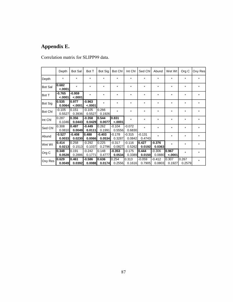
87
Appendix E. Correlation matrix for SLIPP99 data.
Depth Bot Sal Bot T Bot Sig Bot Chl Int Chl Sed Chl Abund Wet Wt Org C Oxy Res
0.682<.0001
-0.765 -0.959<.0001 <.0001
0.535 0.977 -0.9630.0064 <.0001 <.0001
-0.105 0.151 -0.105 0.2660.5527 0.3936 0.5527 0.1926
0.287 0.356 -0.358 0.544 0.8310.1046 0.0443 0.0429 0.0077 <.0001
0.308 0.497 -0.449 0.262 -0.104 -0.0720.0810 0.0049 0.0111 0.1991 0.5556 0.6830
-0.527 -0.408 0.488 -0.403 -0.178 -0.315 -0.1310.0033 0.0230 0.0066 0.0534 0.3287 0.0842 0.4743
0.414 0.258 -0.292 0.225 -0.317 -0.116 0.427 -0.3760.0213 0.1513 0.1037 0.2796 0.0827 0.5262 0.0192 0.0363
0.348 0.191 -0.242 0.148 -0.353 -0.175 0.444 -0.306 0.9670.0528 0.2886 0.1771 0.4777 0.0534 0.3389 0.0150 0.0880 <.0001
0.629 0.461 -0.586 0.636 0.254 0.313 -0.059 -0.412 0.307 0.2670.0049 0.0392 0.0088 0.0174 0.2556 0.1616 0.7905 0.0803 0.1927 0.2579Oxy Res
Wet Wt
Org C
Bot Chl
Int Chl
Sed Chl
Abund
Depth
Bot Sal
Bot T
Bot Sig
* * * * * * * * * * *
* * * * * * * * * *
* * * * * * * * *
* * * * * * * *
* * * * * * *
* * * * * *
* * * * *
* * * *
* * *
* *
*

88
Appendix F. Correlation matrix for HX177 data.
Depth Bot Sal Bot T Bot Sig Bot Chl Int Chl Sed Chl Abund Wet Wt Org C Oxy Res
0.3900.0001
0.327 0.3070.0013 0.0025
0.290 0.953 0.1360.0044 <.0001 0.1806
-0.408 0.114 -0.719 0.249<.0001 0.2672 <.0001 0.0159
0.308 0.102 -0.470 0.129 0.4390.0028 0.3206 <.0001 0.2104 <.0001
-0.029 0.510 -0.501 0.569 0.736 0.3960.8062 <.0001 <.0001 <.0001 <.0001 0.0008
-0.571 -0.316 0.041 -0.232 -0.027 -0.460 -0.243<.0001 0.0154 0.7554 0.0752 0.8356 0.0005 0.0642
0.167 0.257 -0.493 0.376 0.445 0.544 0.514 -0.1300.2005 0.0483 0.0002 0.0039 0.0006 <.0001 <.0001 0.3092
0.142 0.255 -0.461 0.368 0.446 0.511 0.575 -0.130 0.9530.2757 0.0502 0.0004 0.0047 0.0006 <.0001 <.0001 0.3113 <.0001
-0.566 0.213 -0.328 0.002 0.533 0.048 0.556 0.321 0.430 0.393<.0001 0.1137 0.1159 0.9942 <.0001 0.7236 0.0003 0.1732 0.0682 0.0955Oxy Res
Wet Wt
Org C
Bot Chl
Int Chl
Sed Chl
Abund
Depth
Bot Sal
Bot T
Bot Sig
* * * * * * * *
* * *
*
* * * * * *
**
*
*
* * * * * * *
*
*
* * * * * * *
* * * * *
* * * * *
* *
*
* * * * *
* * * *
* *
* *
*
*

89
Vita Jaclyn Leigh Clement was born in Jackson, TN on January 19, 1978. She was
raised in Huntingdon, TN and attended Huntingdon Grade School and Huntingdon Junior
High School. In 1996, she graduated from Huntingdon High School and went on to the
University of Tennessee, Knoxville to obtain a B.S. in Biology in 2000 and a M.S. in
Ecology and Evolutionary Biology with a concentration in Oceanography in August
2002.