USING A LIENARD-WIECHERT SOLVER TO STUDY COHERENTSYNCHROTRON RADIATION EFFECTS

R.D. Ryne∗, C.E. Mitchell, J. Qiang, Lawrence Berkeley National Laboratory, Berkeley, CA, USAB. Carlsten, N. Yampolsky, Los Alamos National Laboratory, Los Alamos, NM, USA

AbstractWe report on coherent synchrotron radiation (CSR)

modeling using a massively parallel, first-principles 3DLienard-Wiechert solver. The solver is able to perform sim-ulations with hundreds of millions to billions of simulationparticles, the same as the real-world number of electronsper bunch typically present in modern accelerators. Wehave recently extended this tool to model a variety of beamtransport systems including undulators. In this paper weprovide an overview of the tool and present several exam-ples. We also describe the concept of a Lienard-Wiechertparticle-mesh (LWPM) code, and how such a code mightmake it possible to perform parallel, self-consistent model-ing using a Lienard-Wiechert approach.

INTRODUCTIONParticle accelerators are among the versatile and impor-

tant tools of scientific discovery and technology advance-ment. They are responsible for a wealth of advances in ma-terials science, chemistry, bioscience, high-energy physics,and nuclear physics. They also have important applicationsto the environment, energy, national security, and medicine.Given the enormous benefit of particle accelerators andtheir extreme complexity, high performance computing us-ing parallel computers has become an essential tool fortheir design and optimization to reduce cost and risk, max-imize performance, and explore advanced concepts.

Early examples of parallel simulation in the U.S. ac-celerator community date from the late 1980’s and early1990’s [1]. By the mid-1990’s parallel beam dynamicscodes had been developed to run on the Thinking Ma-chines CM-5 computer at LANL’s Advanced ComputingLaboratory [2, 3]. In 1997 the U.S. Department of Energy(DOE) approved a “Grand Challenge” project in Compu-tational Accelerator Physics [4]. This later evolved into aDOE Scientific Discovery through Advanced Computing(SciDAC) project [5, 6]. This, as well as other R&D ef-forts in parallel accelerator simulation worldwide, led tothe parallelization of existing beam dynamics codes andthe development of new codes. Examples include ASTRA[7], BeamBeam3D [8], CSRtrack [9], elegant/SDDS [10],GENESIS [11], G4Beamline [12], ICOOL [13], IMPACT[14, 15], MaryLie/IMPACT [16], OPAL [17], SPUR [18],Synergia [19], TRACK [20],TREDI [21], and WARP [22],to name a few.

From the mid-1990’s to the present, significant attentionwas devoted to parallel 3D space-charge modeling, multi-

∗RDRyne@lbl.gov

physics modeling, and increasingly large-scale simulation.In regard to 3D space-charge modeling, many parallel Pois-son solvers were developed to treat a variety of boundaryconditions, e.g., [23, 24, 25]. Integrated Green functions(IGFs) were introduced to increase solver performance andaddress grid aspect ratio issues [26, 27, 28], and are nowused in several codes worldwide [7, 8, 14, 16, 17]. IGFshave also been applied to model 1D CSR [29, 30]. In regardto multi-physics modeling, split-operator methods were in-troduced as a means to combine high-order optics effectswith parallel 3D space-charge and other effects [31], andare used in several codes [14, 16, 17, 19]. In general, paral-lel beam dynamics codes now contain, and are routinelyused to model, a variety of phenomena including high-order optics, space-charge effects, wakefield effects, 1-DCSR effects, electron-cloud effects, and beam-material in-teractions. Regarding the trend toward increasingly large-scale simulation, a start-to-end 2-billion-particle simula-tion of a future light source, based on the single parallelexecutable containing IMPACT-T, IMPACT-Z, and GENE-SIS, requires 10 hours on 2048 cores [32].

Despite these major advances in parallel multi-physicsmodeling, the simulation of 3D CSR effects has remaineda major challenge. A first-principles classical treatmentusually involves the Lienard-Wiechert (L-W) formalism.Since this involves quantities when the radiation was emit-ted (i.e. at retarded times and locations), it requires storinga history of each particle’s trajectory. Also, CSR phenom-ena can exhibit large fluctuations which are physical, notnumerical, hence it is often necessary to use a large numberof simulation particles if those fluctuations are to be mod-eled correctly. Storing a large number of particles over alengthy time history imposes a huge memory requirement.Furthermore the calculation of retarded quantities is itera-tive and extremely time consuming. Consider that the cal-culation of an electric field component on a grid in an elec-trostatic code, e.g., x/|r|3, requires only a small numberof floating point operations at each grid point; by contrastthe calculation of the L-W field at just a single grid pointrequires a small simulation code itself to implement the it-eration to find the retarded quantities, and furthermore theiteration involves numerical integration of trajectories. Insummary a L-W solver involves large memory and manyfloating point operations, and obviously requires parallelcomputing. In addition, to embed such a capability in aself-consistent beam dynamics code would greatly com-pound the computational requirements.

Despite these computational challenges, in the followingwe will present results that point to the possibility of a mas-

Proceedings of FEL2013, New York, NY, USA MOOCNO04

Beam Physics for FEL

ISBN 978-3-95450-126-7

17 Cop

yrig

htc ○

2013

CC

-BY-

3.0

and

byth

ere

spec

tive

auth

ors

sively parallel L-W-based beam dynamics code. First, wewill provide an overview of our parallel L-W solver. Nextwe will provide some example applications to illustrate theusefulness of this approach. Lastly, we will provide an out-line of how standard particle-mesh (PM) techniques used inparallel electrostatic or quasi-electrostatic particle-in-cellcodes can be modified to produce a self-consistent Lienard-Wiechert particle-mesh (LWPM) code.

LIENARD-WIECHERT SOLVERWe begin with the Lienard-Wiechert fields in free space:

~E =

[q

γ2κ3R2

(n̂− ~β

)+

q

κ3Rcn̂×

{(n̂− ~β

)× ∂~β

∂t

}]~B = n̂× ~E (1)

where square brackets denote that the quantity inside is tobe evaluated at the retarded time. In the above, ~β denotesa particle’s velocity vector divided by the speed of light,~R is a vector pointing from a radiating particle’s positionat the retarded time to the observation point at time t, n̂is the unit vector n̂ = ~R/ |R|, and κ = 1 − n̂ · ~β. Fora given observation point (x, y, z) and observation time t,the retarded quantities satisfy,

(x−xr)2 +(y− yr)2 +(z− zr)2− c2(t− tr)2 = 0, (2)

where (xr, yr, zr) denotes a particle’s position at the re-tarded time tr. Note that other boundary conditions can betreated if the underlying Green function is known. For ex-ample, conducting plate boundary conditions can be treatedusing the fields associated with Eq. 4.2 of [33].

In a previous note we reported on calculations based onan electron bunch in a uniform magnetic field [34]. Herewe describe a methodology to treat arbitrary beamlines.Suppose each particle’s evolution is described by a six-vector ζ as a function of some independent variable, τ .Suppose also that each particle’s history has been storedat a number of locations, i.e., suppose that for each particlewe know a sequence, ζk, for k values of the independentvariable τ .

In our Lienard-Wiechert solver, for a given observationpoint, we loop over particles and for each particle we firstfind adjacent quantities k, k+1 that bracket tr. This is doneusing a bisection search to locate a change of sign in Eq. (2)at the stored values. We then use Brent’s method (routinezbrent from [35]) to iteratively find the root of Eq. (2).We have found this approach to be more robust to round-off than a simple Newton search. During the iteration weneed to perform numerical integration of the equations ofmotion between two stored history values. For this purposewe use a Dormand-Prince 8-5-3 algorithm with automaticstep size adjustment [36]. After the iteration has convergedto the retarded quantities we evaluate Eq. (1) to obtain theL-W fields due to each particle. In the following tr is cal-culated to a relative accuracy of 10−10. For some problemswe have found it useful to use extended precision to ensurethat roundoff is not noticeable. For this purpose we use

DDFUN90 package for double-double arithmetic [37]. Oursolver is an MPI code that uses particle decomposition. As-suming the observation points are replicated on the proces-sors, the total L-W fields are found by an MPI reductionthat adds the contributions from all MPI processes. Laterwe will discuss an alternative approach that uses domaindecomposition.

APPLICATIONSAs mentioned previously, in [34] we focused on steady-

state CSR in dipoles. We used a L-W solver to explorelimits of the 1D model, the strength of fluctuations dueto shot noise, and the enhancement of dipole CSR whena bunch has a microbunched structure. In the following wewill present new examples involving dipole CSR, and ex-amples involving undulator radiation. Except where noted,the field plots that follow present just the L-W radiationcomponent. Also, the retarded quantities are computed byintegrating trajectories through just the external fields, notincluding the self-fields.

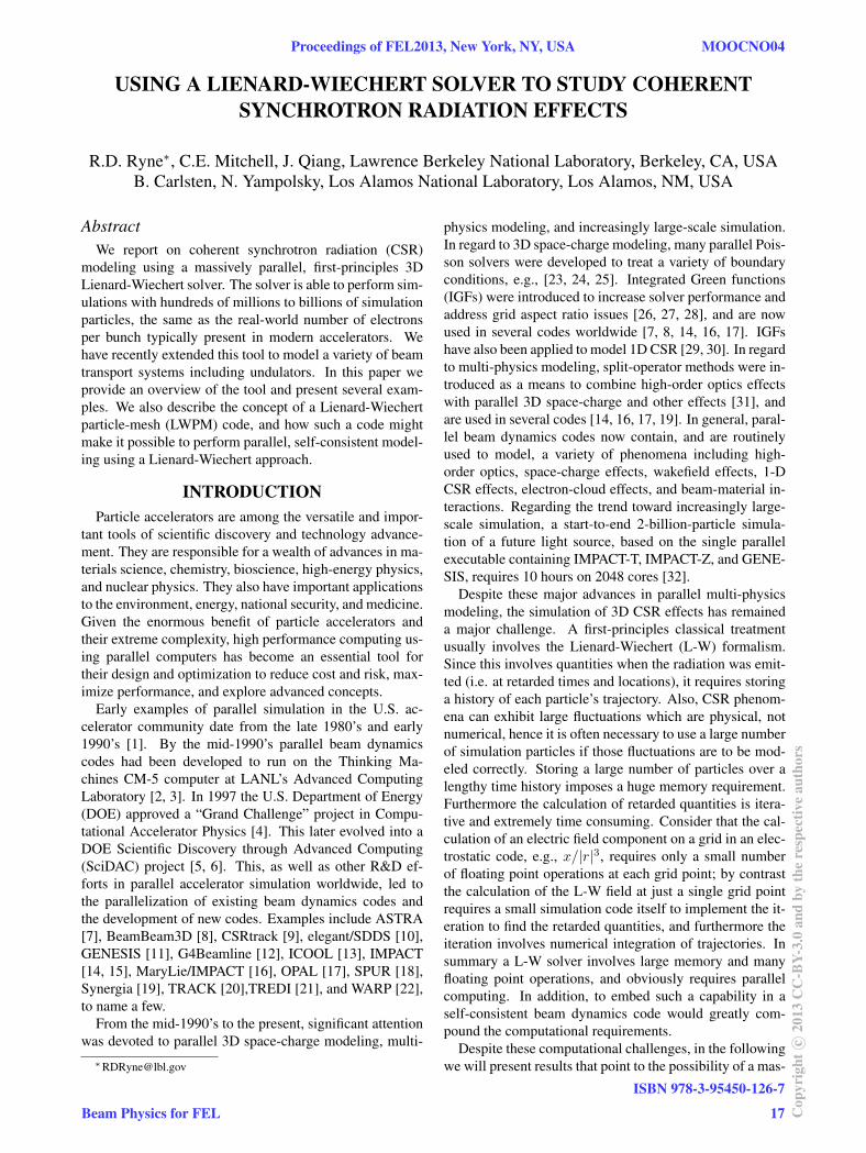
CSR in DipolesFigure 1 shows the results from 6 simulations, each

with 6.24 billion particles (corresponding to 1 nC), ofa zero emittance, 1 GeV bunch in a dipole with ρ =1 m. Starting from a 1x1x10 micron Gaussian bunch,we multiplied the longitudinal distribution by a functiona + b sin(2πz/λmod), where λmod denotes a modulationwavelength, and with a and b chosen so that the amplitudevaried from 0.1 to 1. We randomly sampled the distributionusing a rejection method. Figure 1 shows the longitudinalradiation electric field, Ez,rad for λmod = 5, 10, 50, 100,500 nm. The curve labeled DC has no modulation, i.e., thelongitudinal profile is a Gaussian. Since no adequate theorycan predict the wavelength dependence of CSR enhance-ment, except in some regimes, large-scale L-W simulationprovides a useful means to explore this phenomenon.

Figure 1: Longitudinal radiation electric field, Ez,rad fora 1 GeV bunch with an imposed longitudinal density mod-ulation, simulated with 6.24 billion electrons, for differentvalues of the modulation wavelength.

MOOCNO04 Proceedings of FEL2013, New York, NY, USA

ISBN 978-3-95450-126-7

18Cop

yrig

htc ○

2013

CC

-BY-

3.0

and

byth

ere

spec

tive

auth

ors

Beam Physics for FEL

In [34] we also showed that the 1D model of CSR wasremarkably robust, that only when a Gaussian bunch be-comes extremely flattened (“plate-like”) does the 1D modelbreak down. However, it is worth pointing out that thereare 3D effects that cannot be captured by the 1D model.An example is shown in Fig. 2. In this figure, the bunchis microbunched at λmod = 100 nm. The bunch rms di-mensions in x-y-z (without microbunching) are shown for4 cases: 10x10x10 micron, 10x1x10 micron, 1x10x10 mi-cron, and 1x1x10 micron. As is clear from the figure,the microbunching enhancement is sensitive to the verti-cal bunch size but not to the horizontal bunch size. Suchstudies could not be carried out with a 1D CSR model.

Figure 2: Microbunching field enhancement for differenttransverse bunch sizes. The microbunching enhancementis seen to be sensitive to the vertical bunch size but not tothe horizontal bunch size.

Before leaving the topic of dipole CSR we will presentone more example. Consider the evolution of a test parti-cle moving in the CSR field. Figure 3 shows the tangentialelectric field that would be experienced by a test particleat the center of a 1 GeV, 624M electron, 10x10x10 micronGaussian bunch as it travels through 3 degrees of transportin a magnet with ρ = 1m. As can be seen in the inset, theshot noise fluctuations are very well resolved. Using thisdata we computed its autocorrelation function and exam-ined its dependence on energy. Figure 4 shows the energychange as a function of propagation distance in the dipolethat would be experienced by a test particle at the centerof the bunch. The bunch is a zero emittance, 1 GeV, 1nCGaussian with rms sizes σx = σy = σz = 10micron. The4 curves correspond to 4 different realizations of the distri-bution, each modeled with 6.24 billion particles. The timehistories corresponding to different realizations of the shotnoise seem independent from each other and can be rea-sonably approximated by a random walk model. The reddashed lines show the boundaries that the energy changeshould satisfy if the process is diffusive. The diffusion co-efficient was calculated based on the autocorrelation func-tion of the energy time history.

Figure 3: Tangential electric field at the center of a 1 GeV,624M electron, 10x10x10 micron Gaussian bunch as ittravels through 3 degrees of transport in a magnet withρ = 1 m. The narrow blue rectangle shows the domainof the inset, indicating that the fluctuations are very wellresolved.

0 0.5 1 1.5 2 2.5 3−800

−600

−400

−200

0

200

400

600

800

1000

e [deg]

6E

[eV]

Figure 4: Energy change of a particle at the bunch centervs. propagation distance in a dipole, computed using thetangential electric field produced by the L-W solver. The4 curves correspond to 4 different realizations of the distri-bution, each modeled with 6.24 billion particles. The reddashed lines show the boundaries that the energy changeshould satisfy if the process satisfies a diffusion equation.

Undulator RadiationThe following results are based on an undulator field that

is given by,By = B0 sin(kwz), (3)

where B0 is the peak magnetic field in the y-direction,and where kw = 2π/λw is the undulator wave number.The particles travel along the z-direction and wiggle in thex − z plane. This undulator model has no entrance or exitfields. However, since our simulation finds retarded quan-tities though high-order numerical integration [36], and not

Proceedings of FEL2013, New York, NY, USA MOOCNO04

Beam Physics for FEL

ISBN 978-3-95450-126-7

19 Cop

yrig

htc ○

2013

CC

-BY-

3.0

and

byth

ere

spec

tive

auth

ors

by simple analytic approximations of trajectories in the un-dulator, this approach could equally well be applied to anyundulator model whose fields are known analytically or areaccessible by some numerical procedure.

Before presenting multi-particle simulation results, firstconsider the single-particle wakefields. Figure 5 showsthe radiation component of Ex for a 125 MeV electronin an undulator with B0 = .025 T and λw = 3 cm.For these parameters the undulator K-value is 0.07. Notethat the wavelength of the oscillation in Fig. 5 is approx-imately 0.25 micron, consistent with the expected valueλu/(2γ

2)(1 + K2/2) = 0.249 micron. Figure 6 showsthe same quantities for a 14 GeV electron in an undulatorwith B0 = 1.3 T and kw = 3 cm. For these parameters theundulator K-value is comparable to LCLS, K = 3.64. Asseen in Fig. 6, the oscillation wavelength is approximately1.53 Angstrom, consistent with the expected value 1.525Angstrom. The wake for this case contains a lot of highharmonics unlike the previous case with K�1. The peakat the origin has a value 1.9e10 V/m, while the peak is only263 V/m in the preceding figure. In both these figures itis understood that the fields are plotted at t = 0 when theelectron is at x = y = z = 0 (and dx/dt chosen to pro-duce a periodic orbit). The time-dependent wakefield is ofcourse oscillatory with a frequency equal to the electrontravel time over an undulator period.

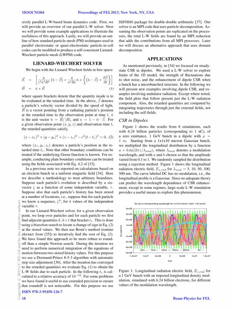
Returning to the 125 MeV case, next consider a Gaussianbunch of electrons with rms sizes σx = σy = σz = 10 µmpropagating along the undulator. The simulations that fol-low used only 24 million electrons. Figure 7 shows theradiation component of Ex produced by this bunch. It isinteresting to note that the shot noise fluctuations are small,much smaller than those presented in [34] for the steady-state dipole CSR case. This is understood to be due tothe fact that all the particles in the undulator radiate in-side a cone that is smaller than the wiggle amplitude, incontrast to the dipole case for which the particles radiatealong an extended path whose opening angle is much largerthan the radiation cone angle. Though the fluctuations aresmall, they are still present, as seen in Fig. 8 which showsa zoomed-in view. Another observation in Fig. 7 is that theradiation pattern follows the bunch profile, i.e., there is noradiation produced ahead the bunch itself. Next, supposethat the Gaussian bunch is microbunched at a modulationwavelength λmod = 0.249 micron. Figure 9 shows the sim-ulation results. Now it is clear that there is a strong radia-tion field ahead of the bunch. The oscillation is evident inthe inset of the figure.

CONVOLUTION-BASED SOLVERThe preceding results were all based on computing the

exact L-W fields at an observation point by summing thecontributions from N particles. In an N-body code thiswould scale as N2 which is huge considering that N is oforder 109. Now we will consider an alternative method tocomputing the L-W fields from a distribution of particles.Instead of summing N Green functions at a point (i.e. the

Figure 5: x-component of the single-particle radiation elec-tric field, Ex,rad, for a 125MeV electron inside an undu-lator with B0 = 0.025 T and λw = 3 cm, correspondingto an undulator K value of 0.07 .

Figure 6: x-component of the single-particle radiation elec-tric field,Ex,rad, for a 14GeV electron inside an undulatorwith B0 = 1.3 T and λw = 3 cm, corresponding to an un-dulator K value of 3.64 .

L-W fields of N point-particles), we use just one Greenfunction, and convolve it with the charge density at the ob-servation time. This method has the advantage that just oneGreen function needs to be calculated (rather than of order109). Furthermore, by zero-passing the charge density (see,e.g., the appendix in [38]), the convolution can be perform-ing using an FFT-based method, which scales as M logM ,where M is the number of grid points. Also, the FFT canbe performed using a parallel FFT routine. This approachis analogous to the method in widely used electrostatic orquasi-electrostatic PIC codes: in that approach, a Lorentz-transformation is used to transform to the bunch frame, theelectrostatic fields are computed based on a single Greenfunction, and the fields are transformed back to the lab-oratory frame. Such an approach is not always valid, aswith some photoinjector simulations where the bunch en-ergy spread is so large that there is no frame of reference

MOOCNO04 Proceedings of FEL2013, New York, NY, USA

ISBN 978-3-95450-126-7

20Cop

yrig

htc ○

2013

CC

-BY-

3.0

and

byth

ere

spec

tive

auth

ors

Beam Physics for FEL

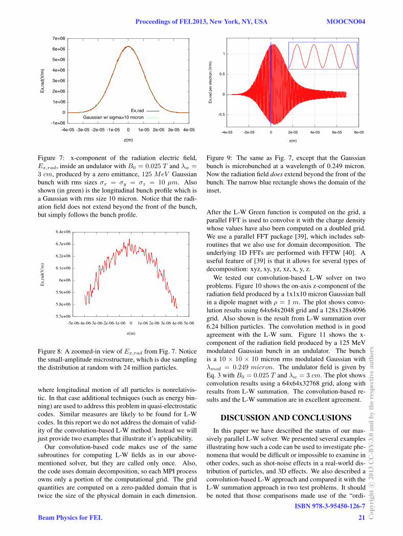
Figure 7: x-component of the radiation electric field,Ex,rad, inside an undulator with B0 = 0.025 T and λw =3 cm, produced by a zero emittance, 125 MeV Gaussianbunch with rms sizes σx = σy = σz = 10 µm. Alsoshown (in green) is the longitudinal bunch profile which isa Gaussian with rms size 10 micron. Notice that the radi-ation field does not extend beyond the front of the bunch,but simply follows the bunch profile.

Figure 8: A zoomed-in view of Ex,rad from Fig. 7. Noticethe small-amplitude microstructure, which is due samplingthe distribution at random with 24 million particles.

where longitudinal motion of all particles is nonrelativis-tic. In that case additional techniques (such as energy bin-ning) are used to address this problem in quasi-electrostaticcodes. Similar measures are likely to be found for L-Wcodes. In this report we do not address the domain of valid-ity of the convolution-based L-W method. Instead we willjust provide two examples that illustrate it’s applicability.

Our convolution-based code makes use of the samesubroutines for computing L-W fields as in our above-mentioned solver, but they are called only once. Also,the code uses domain decomposition, so each MPI processowns only a portion of the computational grid. The gridquantities are computed on a zero-padded domain that istwice the size of the physical domain in each dimension.

Figure 9: The same as Fig. 7, except that the Gaussianbunch is microbunched at a wavelength of 0.249 micron.Now the radiation field does extend beyond the front of thebunch. The narrow blue rectangle shows the domain of theinset.

After the L-W Green function is computed on the grid, aparallel FFT is used to convolve it with the charge densitywhose values have also been computed on a doubled grid.We use a parallel FFT package [39], which includes sub-routines that we also use for domain decomposition. Theunderlying 1D FFTs are performed with FFTW [40]. Auseful feature of [39] is that it allows for several types ofdecomposition: xyz, xy, yz, xz, x, y, z.

We tested our convolution-based L-W solver on twoproblems. Figure 10 shows the on-axis z-component of theradiation field produced by a 1x1x10 micron Gaussian ballin a dipole magnet with ρ = 1 m. The plot shows convo-lution results using 64x64x2048 grid and a 128x128x4096grid. Also shown is the result from L-W summation over6.24 billion particles. The convolution method is in goodagreement with the L-W sum. Figure 11 shows the x-component of the radiation field produced by a 125 MeVmodulated Gaussian bunch in an undulator. The bunchis a 10 × 10 × 10 micron rms modulated Gaussian withλmod = 0.249 micron. The undulator field is given byEq. 3 with B0 = 0.025 T and λw = 3 cm. The plot showsconvolution results using a 64x64x32768 grid, along withresults from L-W summation. The convolution-based re-sults and the L-W summation are in excellent agreement.

DISCUSSION AND CONCLUSIONSIn this paper we have described the status of our mas-

sively parallel L-W solver. We presented several examplesillustrating how such a code can be used to investigate phe-nomena that would be difficult or impossible to examine inother codes, such as shot-noise effects in a real-world dis-tribution of particles, and 3D effects. We also described aconvolution-based L-W approach and compared it with theL-W summation approach in two test problems. It shouldbe noted that those comparisons made use of the “ordi-

Proceedings of FEL2013, New York, NY, USA MOOCNO04

Beam Physics for FEL

ISBN 978-3-95450-126-7

21 Cop

yrig

htc ○

2013

CC

-BY-

3.0

and

byth

ere

spec

tive

auth

ors

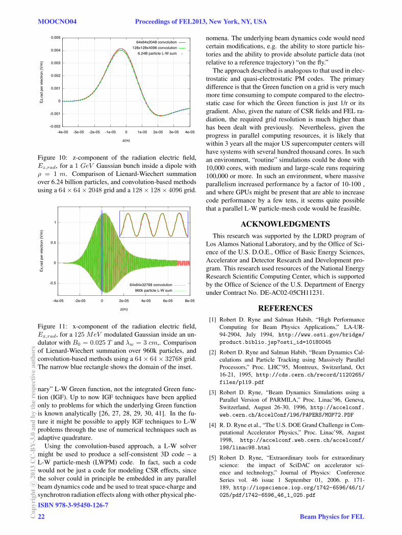
Figure 10: z-component of the radiation electric field,Ez,rad, for a 1 GeV Gaussian bunch inside a dipole withρ = 1 m. Comparison of Lienard-Wiechert summationover 6.24 billion particles, and convolution-based methodsusing a 64× 64× 2048 grid and a 128× 128× 4096 grid.

Figure 11: x-component of the radiation electric field,Ex,rad, for a 125MeV modulated Gaussian inside an un-dulator with B0 = 0.025 T and λw = 3 cm,. Comparisonof Lienard-Wiechert summation over 960k particles, andconvolution-based methods using a 64× 64× 32768 grid.The narrow blue rectangle shows the domain of the inset.

nary” L-W Green function, not the integrated Green func-tion (IGF). Up to now IGF techniques have been appliedonly to problems for which the underlying Green functionis known analytically [26, 27, 28, 29, 30, 41]. In the fu-ture it might be possible to apply IGF techniques to L-Wproblems through the use of numerical techniques such asadaptive quadrature.

Using the convolution-based approach, a L-W solvermight be used to produce a self-consistent 3D code – aL-W particle-mesh (LWPM) code. In fact, such a codewould not be just a code for modeling CSR effects, sincethe solver could in principle be embedded in any parallelbeam dynamics code and be used to treat space-charge andsynchrotron radiation effects along with other physical phe-

nomena. The underlying beam dynamics code would needcertain modifications, e.g. the ability to store particle his-tories and the ability to provide absolute particle data (notrelative to a reference trajectory) “on the fly.”

The approach described is analogous to that used in elec-trostatic and quasi-electrostatic PM codes. The primarydifference is that the Green function on a grid is very muchmore time consuming to compute compared to the electro-static case for which the Green function is just 1/r or itsgradient. Also, given the nature of CSR fields and FEL ra-diation, the required grid resolution is much higher thanhas been dealt with previously. Nevertheless, given theprogress in parallel computing resources, it is likely thatwithin 3 years all the major US supercomputer centers willhave systems with several hundred thousand cores. In suchan environment, “routine” simulations could be done with10,000 cores, with medium and large-scale runs requiring100,000 or more. In such an environment, where massiveparallelism increased performance by a factor of 10-100 ,and where GPUs might be present that are able to increasecode performance by a few tens, it seems quite possiblethat a parallel L-W particle-mesh code would be feasible.

ACKNOWLEDGMENTSThis research was supported by the LDRD program of

Los Alamos National Laboratory, and by the Office of Sci-ence of the U.S. D.O.E., Office of Basic Energy Sciences,Accelerator and Detector Research and Development pro-gram. This research used resources of the National EnergyResearch Scientific Computing Center, which is supportedby the Office of Science of the U.S. Department of Energyunder Contract No. DE-AC02-05CH11231.

REFERENCES[1] Robert D. Ryne and Salman Habib, “High Performance

Computing for Beam Physics Applications,” LA-UR-94-2904, July 1994, http://www.osti.gov/bridge/

product.biblio.jsp?osti_id=10180045

[2] Robert D. Ryne and Salman Habib, “Beam Dynamics Cal-culations and Particle Tracking using Massively ParallelProcessors,” Proc. LHC’95, Montreux, Switzerland, Oct16-21, 1995, http://cds.cern.ch/record/1120265/

files/p119.pdf

[3] Robert D. Ryne, “Beam Dynamics Simulations using aParallel Version of PARMILA,” Proc. Linac’96, Geneva,Switzerland, August 26-30, 1996, http://accelconf.

web.cern.ch/AccelConf/l96/PAPERS/MOP72.PDF

[4] R. D. Ryne et al., “The U.S. DOE Grand Challenge in Com-putational Accelerator Physics,” Proc. Linac’98, August1998, http://accelconf.web.cern.ch/accelconf/

l98/linac98.html

[5] Robert D. Ryne, “Extraordinary tools for extraordinaryscience: the impact of SciDAC on accelerator sci-ence and technology,” Journal of Physics: ConferenceSeries vol. 46 issue 1 September 01, 2006. p. 171-189, http://iopscience.iop.org/1742-6596/46/1/

025/pdf/1742-6596_46_1_025.pdf

MOOCNO04 Proceedings of FEL2013, New York, NY, USA

ISBN 978-3-95450-126-7

22Cop

yrig

htc ○

2013

CC

-BY-

3.0

and

byth

ere

spec

tive

auth

ors

Beam Physics for FEL

[6] Ji Qiang et al., “SciDAC Advances in Beam Dynam-ics Simulation: From Light Sources to Colliders,”Journal of Physics: Conference Series vol. 125, Sci-DAC 2008, 13-17 July 2008, Seattle, WA, USA,http://iopscience.iop.org/1742-6596/125/1/

012004/pdf/1742-6596_125_1_012004.pdf

[7] http://tesla.desy.de/~meykopff/

[8] http://amac.lbl.gov/~jiqiang/BeamBeam3D/

[9] http://www.desy.de/xfel-beam/csrtrack/

[10] http://aps.anl.gov/elegant.html

[11] http://genesis.web.psi.ch

[12] http://www.muonsinternal.com/muons3/

G4beamline

[13] http://www.cap.bnl.gov/ICOOL/

[14] http://amac.lbl.gov/~jiqiang/IMPACT/

[15] http://amac.lbl.gov/~jiqiang/IMPACT-T/

[16] R. D. Ryne et al., “Recent Progress on theMaryLie/IMPACT Beam Dynamics Code,” Proceedings ofICAP 2006, Chamonix, France, http://accelconf.web.cern.ch/accelconf/ICAP06/PAPERS/TUAPMP03.PDF

[17] A. Adelmann et al., “The Object Oriented Parallel Acceler-ator Library (OPAL), Design, Implementation and Applica-tion,” Proc. ICAP09, San Francisco, CA, USA

[18] N. C. Ryder, D. J. Scott, and S. Reiche, “SPUR: A NewCode for the Calculation of Synchrotron Radiation fromVery Long Undulator Systems,” Proc. EPAC08, Genoa, Italy

[19] J. Amundson et al., “Synergia: A 3D Accelerator Mod-elling Tool with 3D Space Charge. Journal of ComputationalPhysics,” Volume 211, Issue 1 , 1 January 2006, Pages 229-248.

[20] P. Ostroumov at al., “TRACK, The Beam Dynamics Code”,Proc. PAC2005

[21] L. Giannessi and M. Quattromini, “TREDI Simulationsfor High-brilliance Photoinjectors and Magnetic Chicanes,”Phys.Rev. ST-AB 6 120101 (2003)

[22] D.P. Grote, A. Friedman, I. Haber, Methods used inWARP3d, a Three-Dimensional PIC/Accelerator Code,Proc. of the 1996 Comp. Accel. Physics Conf., AIP Con-ference Proceedings 391, p . 51 (1996).

[23] Ji Qiang and Robert D. Ryne, “Parallel 3D Poisson solverfor a charged beam in a conducting pipe,” Comp. Phys.Comm. 138, pp 18-28, 2001.

[24] G. Poplau, U. van Rienen, K. Flottmann, “The Performanceof 3D Space Charge Models for High Brightness ElectronBunches,” TUPP103, Proc. EPAC08, Genoa, Italy

[25] A. Adelmann, P. Arbenz, and Y. Ineichen, “A Fast ParallelPoisson Solver on Irregular Domains Applied to Beam Dy-namic Simulations,” arXiv:0907.4863, February 2010

[26] Robert D. Ryne, “A new technique for solving Poissonsequation with high accuracy on domains of any aspect ratio,ICFA Beam Dynamics Workshop on Space-Charge Simula-tion, Oxford, April 2-4, 2003.

[27] J. Qiang, M. A. Furman, R. D. Ryne, W. Fischer, K. Ohmi,“Recent advances of strong-strong beam-beam simulation,”Nuclear Instruments & Methods in Physics Research A558,351, (2006).

[28] D.T. Abell et al.,“Three-Dimensional Integrated GreenFunctions for the Poisson Equation,” Proc. PAC2007, 3546-3548.

[29] R. D. Ryne, B. Carlsten, J. Qiang, and N. Yampolsky, “Amodel for one-dimensional coherent synchrotron radiationincluding short-range effects,” http://arxiv.org/abs/

1202.2409

[30] C. Mitchell, J. Qiang, and R. Ryne, “A Fast Method forComputing 1-D Wakefields due to Cohereent SynchrotronRadiation,” Nucl. Instrum. Methods Phys. Res., Sect. A 715,119 (2013)

[31] Robert D. Ryne, Ji Qiang, and Salman Habib, “Compu-tational Challenges in High Intensity Ion Beam Physics,”Proc. 2nd ICFA Advanced Accelerator Workshop on thePhysics of High Brightness Beams, World Scientific, JamesRosenzweig & Luca Serafini, Eds., Nov. 9-12, 1999, LosAngeles, CA, USA

[32] J. Qiang, “Start-to-End Simulation of a Next GenerationLight Source Using the Real Number of Electrons,” this pro-ceedings

[33] J. B. Murphy, S. Krinsky, and R. L. Gluckstern, Longitudi-nal Wakefield for an Electron Moving on a Circular Orbit,Particle Accelerators, Vol 57, pp. 9-64, 1997.

[34] R. D. Ryne et al., “Large-Scale Simulation of SynchrotronRadiation using a Lienard-Wiechert Approach,” Proc. IPAC2012, New Orleans, LA, USA, May 2012

[35] William H. Press, Saul A. Teukolsky, William T. Vetterling,Brian P. Flannery, “Numerical Recipes in Fortran 77: TheArt of Scientific Computing,” Cambridge University Press

[36] http://www.unige.ch/~hairer/prog/nonstiff/

dop853.f

[37] http://crd-legacy.lbl.gov/~dhbailey/mpdist/

[38] Robert D. Ryne, “On FFT-based convolutions and correla-tions, with application to solving Poisson’s equation in anopen rectangular pipe,” arxiv.org/pdf/1111.4971

[39] http://www.sandia.gov/~sjplimp/docs/fft/

README.html

[40] http://http://www.fftw.org

[41] Robert D. Ryne, “An Integrated Green Function PoissonSolver for Rectangular Waveguides,” Proc. IPAC 2012, NewOrleans, LA, USA, May 2012

Proceedings of FEL2013, New York, NY, USA MOOCNO04

Beam Physics for FEL

ISBN 978-3-95450-126-7

23 Cop

yrig

htc ○

2013

CC

-BY-

3.0

and

byth

ere

spec

tive

auth

ors