using a non-linear multilayer feedforward neural network

Using a Non-linear MultilayerFeedforward Neural Network for

Ballhandling Control withinRoboCup Middle Size League

Eindhoven University of Technology

Supervisor: Prof. Valeri MladenovCourse 5P060

Robin Soetens (0631301)

January 31, 2012

Abstract

Soccer playing robots of team Tech United Eindhoven have active ballhandling controlin place for four years now. Two drawbacks of the current method are identified: (i) Smallchanges in hardware or environment cause the need to regularly re-tune the system and(ii) ballhandling dynamics are non-linear, complicating modeling and control design. In thisreport first steps are made to investigate whether a neural network can do better than this. Anon-linear multilayer feedforward neural network was trained to imitate the original, model-based, controller. By implementing the network with trained weights on the robot itself,performance was validated. In the final section of this report suggestions are made on howto use neural networks within different frameworks for self-learning.

Keywords: Non-linear Neural Network, Neural Control, Backpropagation, Ballhandling,RoboCup Middle Size, Neural Fitted Q-iteration

The title page depicts an autonomous soccer playing robot of team Tech United, notethere is a list of symbols attached in the back of this report. All code and logged dataused for experiments is available via http://goo.gl/pf9i0. Questions can be directed [email protected]

http://goo.gl/pf9i0

Contents

1 Introduction 2

2 Problem Statement 5

3 Method 73.1 Multilayer non-linear feedforward network . . . . . . . . . . . . . . . . . . . . 93.2 Pseudocode . . . . . . . . . . . . . . . . . . . . . . . . . . . . . . . . . . . . . 113.3 Convergence . . . . . . . . . . . . . . . . . . . . . . . . . . . . . . . . . . . . . 12

4 Results 144.1 Stationary Robot . . . . . . . . . . . . . . . . . . . . . . . . . . . . . . . . . . 144.2 Robot moving around . . . . . . . . . . . . . . . . . . . . . . . . . . . . . . . 20

4.2.1 Linear Network . . . . . . . . . . . . . . . . . . . . . . . . . . . . . . . 214.2.2 Non-linear Network . . . . . . . . . . . . . . . . . . . . . . . . . . . . 23

4.3 Real-time implementation . . . . . . . . . . . . . . . . . . . . . . . . . . . . . 25

5 Future work 275.1 Neural system identification . . . . . . . . . . . . . . . . . . . . . . . . . . . . 285.2 Neural Fitted Q-Iteration . . . . . . . . . . . . . . . . . . . . . . . . . . . . . 28

6 Conclusion 30

A List of symbols used in text 34

B Logging data 35B.1 Robot at standstill . . . . . . . . . . . . . . . . . . . . . . . . . . . . . . . . . 36B.2 Moving robot . . . . . . . . . . . . . . . . . . . . . . . . . . . . . . . . . . . . 36

C Neural network code, three different implementations 38C.1 Simulink S-function . . . . . . . . . . . . . . . . . . . . . . . . . . . . . . . . . 38C.2 Standalone executable . . . . . . . . . . . . . . . . . . . . . . . . . . . . . . . 45C.3 M-file implementation . . . . . . . . . . . . . . . . . . . . . . . . . . . . . . . 53

D Neural network code (real-time implementation) 58

1

Chapter 1

Introduction

RoboCup is an international federation of academics promoting development of autonomousrobotics via competition in different leagues.1 Most of them involve robotic soccer playing.Tech United is a TU/e team participating in the RoboCup middle size league competition.Its autonomous soccer playing robots rank among the top teams worldwide [4].

Of all RoboCup soccer competitions, the middle size league is as close as it gets to actualsoccer. The rulebook of this competition is a slightly adapted version of the official FIFArulebook, which makes middle size league matches dynamic and exiting to watch for a broadaudience. During a match, four autonomous field players and a goalkeeper have to cooperatethrough a wifi connection in order to beat the opponent.

Each team is allowed to design its own robot but within certain boundaries with respectto weight and size. Tech United uses an omnivision unit to distinguish the ball, opponentsand the lines of the field. Furthermore a triangular setup of omniwheels is designed such thatthe robot is able to move around freely. In order to kick the ball, a large solenoid actuates ashooting lever (Fig. 1.1). Powerful actuators can make the 35 kg robot drive with up to fourmeters per second velocity and shooting speeds of ten meters per second are reached.

An essential part of the design is the mechanism that controls the ball. Rules prescribethat the robot is not allowed to touch or enclose more than a third of the balls surface andthat it is not allowed to ’grasp’ the ball while moving around. In other words: Opponentplayers should always have the possibility to steal the ball from another robot and the ballshould roll naturally in front of the robot controlling it.

Having a good ballhandling mechanism is not only important in reaching the opponentsgoal. During scrum situations, a lot of robots try to gain possession of the ball. The one whois able to control the ball best, will eventually obtain possession. Also when intercepting aloose ball, it is essential to be able to immediately control the ball.

Tech Uniteds soccer robot has active ballhandling in place for four years now.2 Controlfor this ballhandling is designed model based. For reasons stated in the next chapter, it isinteresting to investigate whether a neural network can do better than this.

Historically, the topic of neural networks regularly becomes ’trending’. With promisingdevelopment of perceptron learning, Hebbs rule and the McCulloch-Pitts neuron in the 1950sand 1960s, this period is described as ’The Golden Age of Neural Networks’ [6]. Hereafter aquit period passed but because of increased mathematical understanding of backpropagation

1RoboCup federation official website http://www.robocup.org2Videos of the current ballhandling in action at http://www.techunited.nl

2

http://www.robocup.org

http://www.techunited.nl

Figure 1.1: Picture of the soccer robot without covers, the watermelon is placed where therobot normally controls the ball.

3

algorithms in the 1980s, interest was reborn.During the first golden age of neural networks, statistical learning theory was developed

that thirty years later would form the base for a new class of methods called ’support vec-tor machines’ [17]. This method could be interpreted being a non-linear extension of theperceptron learning developed in the first golden age. Advances like SVM, but also the in-creased public interest in robotics and artificial intelligence research [7], have boosted neuralnetworks research in the past twenty years. We might be experiencing the next golden ageof neural networks right now! Recent breakthroughs in the field are for example within thefield of reservoir computing [3]. In most cases this type of computing is used to solve patternrecognition problems like, for example, speech recognition. The neural networks applicationinvestigated in this assignment is a different one though.

In this report, the neural network is used as a controller for a motion system. Thereforethe use of the net is entirely different. Instead of mapping a continuous input to a set of cases(pattern recognition), the net maps a continuous input to a continuous output/control signal.The ability to represent non-linear functions and the possibility to automatically adapt thecontrol policy over time are two reasons to study neural networks for control.

During the assignment we chose not to use an of the shelve API for neural networks.3 Inorder to fully understand the algorithm we hand coded every step of the code. Also a detailedmathematical description of the update rule has been incorporated in this report.

3’Cortex ANN Software’ can be used as a C++ API for backpropagation neural networks http://cortex.

snowcron.com/cortex.htm. Also there exists a Matlab toolbox for neural networks

4

http://cortex.snowcron.com/cortex.htm

http://cortex.snowcron.com/cortex.htm

Chapter 2

Problem Statement

As mentioned in the introduction, the ballhandling mechanism is essential to success withinthe RoboCup middle size league. Tech United’s soccer robots are provided with two movablelevers to manipulate the ball while dribbling (Fig. 2.1). Using both feedforward and a feed-back loop, the velocity of a wheel on each lever is controlled such that the ball rolls naturallywhile the robot is moving around. The feedforward loop uses the velocity of the robot itselfas an input, while the feedback loop uses the error between a predefined reference positionfor the ballhandling levers and the actual ball position [2]. A more accurate explanation ofthe current ballhandling control software is given in chapter 4.

Two drawbacks of the controller that is currently implemented are: (i) Over the courseof time and in different situations, the ballhandling hardware changes, requiring additionaltuning, e.g., changes in friction between wheels and ball, or between the ball and carpet, anddeterioration of the lever positions as a result of wear and collisions. (ii) The dynamics of theballhandling system are non-linear, complicating modeling and control design. Consequently,additional non-model-based and non-linear control effort is used in specific situations, e.g., ascrum situation or during sharp turns of the robot around its vertical axis.

As a result, tuning of the controller parameters is time consuming, requiring much effortand insight in the system characteristics. Neural network algorithms theoretically can solveabove mentioned problems. By learning a set of weights that map a number of inputs to anoptimal ballhandling velocity, a neural net could take care of tuning ’on-line’. The seconddrawback of the current controller could be solved by neural networks because they are able tomap both linear and non-linear functions. Furthermore by rewarding the learning algorithmfor ’not losing the ball’ instead of ’staying close to the reference position’, it would theoreticallybe possible to discover new control policies without much knowledge of system characteristicsneeded. The knowledge of the system slowly gets incorporated in the neural network.

Many applications of neural networks involve supervised learning, meaning the outcome ofthe net can be compared to some target vector in order to obtain an error value (more aboutthis in chapter 3). In our application, the target vector will be the outcome of the currentballhandling, while logging the robots own velocity and angle of the ballhandling levers asinputs. The weights that are obtained this way will result in a neural ballhandling controllerthat provides exactly the same output as the model-based controller does now.

To meet the first goal of creating ballhandling software that tunes automatically, theseweights will be used as an initial value. At a higher level, a loop should be designed thatbackpropagates an error value continuously adjusting the weights. This updating of weights

5

Figure 2.1: Close up of ballhandling mechanism, directly behind the motor is a tacho thatmeasures velocity.

should happen in real-time, but in a subtle way. Phenomena like the formation of play orfriction coefficients getting affected by wear, occur at time scales that are at least measured inhours (instead of minutes). To meet the second goal, experiments have to be performed withlarger learning rates, training situations for which the ball is lost with the current ballhandlingcontroller.

6

Chapter 3

Method

Neural networks can be classified either by their active phase or by their learning phase.Learning refers to the way the weights in the neural net are updated, which can be donebased on either a supervised or an unsupervised learning algorithm. The active phase refersto the way a network constructs a certain output from the input signal. First we discuss thelearning phase.

Supervised learning is learning from examples. During training, every input vector has acorresponding vector that represents the desired output (the target vector). At first, it seemsto be stupid to start learning something we apparently already know. But imagine a networkbeing trained to recognize black and white images of all letters in the alphabet (Fig. 3.1).The input would then be a long binary vector with each entry corresponding to a pixel (1for a black pixel, 0 for a white one). We choose the output vector to contain 26 entries, witheach entry corresponding to a character we are trying to recognize. After the character isshown, the net should indicate which character it saw by putting a 1 in the correspondingentry of the output vector and leaving all other entries at zero. During training, the weights inthe network are adjusted until the network recognizes all characters. The value of supervisedlearning becomes visible once we provide the net with a noisy input (grey pixels in the bottompart of the figure). The network still is able to recognize the characters! Making use of thetraining examples that were provided, we created a net that is able to also recognize inputsthat are slightly adjusted. It generalizes from the examples it had during the training phase.

A second classification of neural networks is based on the active phase, which can involvefeedforward but also feedback. Neural networks only with feedforward connections are staticmappings, without an internal state. Networks also having feedback loops implemented arecalled ’recursive neural networks’. Output of these networks is not only dependent on thecurrent input but also on its internal state, which is a function of past inputs. Recurrentnetworks are dynamic networks [1], they introduce derivatives.

In order to choose a type of neural network out of many types of networks existing, weshould look at the task the network has to perform. The network should comprehend anon-linear mapping from continuous input signals to continuous output signals. This task isdifferent from the pattern recognition example shown in figure 3.1, where the net is used toseparate input space in a number of different regions. Many types of networks are especiallyintended for these pattern recognition tasks, they don’t result in a continuous output functionand therefore they are not suited. Traditional networks using for example McCulloch-Pittsneurons are not designed for continuous input or output either. In the next section we will

7

Figure 3.1: After supervised learning, the net is able to recognize characters even when pixelsare missing or perceived at the wrong position, also when the network did not see thesespecific disturbances during supervised training.

8

explain how how multiple layers of non-linear nodes can be linked to obtain what beingreferred to ’a multilayer perceptron network’.

3.1 Multilayer non-linear feedforward network

Figure 3.2 depicts a network consisting of three layers with neural nodes. The first layer iscalled the input layer and consist of a bias, the position of the left and right ballhandlinglever (φll and φrl) and the velocity of the robot itself (xrobot, yrobot and θrobot). The layer inthe middle is called ’hidden layer’ and consists of a number of non-linear nodes. At the rightside two non-linear output nodes are shown (φlb and φrb).

Before we start deriving backpropagation rules for this network1, it is useful to introducesome extra notation. The vector containing all six input values is called x, the vector ofhidden layer node outputs is named z and the output layer vector is indicated with y. Weightvij denotes the weight between input node i and hidden node j and wjk represents the weightbetween hidden node j and output node k. The matrix of weights between the input andhidden layer is indicated with V and W is the matrix of weights between the hidden layerand the output layer.

Zooming in at a specific non-linear node (could be any node within the hidden layer oroutput layer), we see the calculation is twofold. First all inputs are summed (Eq. 3.1), thanthis value is put into the so called ’activation function’. Any continuous, bounded, functioncan be chosen as activation function as long as it is a uniform one. Which means that byscaling and translating a large numbers of these functions, any arbitrary continuous non-linearfunction can be covered. Here we chose the hyperbolic tangent (Eq. 3.2), because it is easyto differentiate (which is useful during backpropagation).

zinj =

6∑i=1

(xi · vij) (3.1)

zj = tanh(zinj ) (3.2)

The procedure for the entire network follows from this single node example directly. Firstall hidden layer inputs zin are calculated by a matrix multiplication 3.3.

zin = V · x (3.3)

Hereafter the activation function is applied to each hidden layer element to obtain z andthe yin values are determined by equation 3.4.

yin = W · z (3.4)

After applying the activation function once again, y is obtained. It consists of the twodesired velocities for the ballhandling wheels.

Now that the activation phase is explained, let us have a look at the learning phase. Sincethere is a target vector (t) available, consisting of the output of the current, model-based,ballhandling controller, we can make use of error backpropagation. First we have to definethe error, which we do as in equation 3.5 such that it is possible to differentiate it twice

1Theory in this section based on sheets of course 5P060 ’Nonlinear systems and Neural Networks’, PartII-1, taught by Prof. V. Mladenov in 2011

9

Figure 3.2: Multilayer feedforward non-linear neural network for ballhandling control, thedotted box shows what is happening inside a non-linear node. Values in the input layer arestored in vector x, values of the middle (hidden) layer are stored in z and values in the outputlayer in y. Later on (section 4.1) we would find out also the rotational velocity measured bythe ballhandling tachos should be provided to the network. Furthermore we decided to omitthe activation function at the output layer to provide the network with more freedom.

10

with respect to a specific weight. The quadratic term also makes the error sign independent,judging performance we don’t care whether the value is too high or too low.

E =1

2

2∑k=1

(tk − yk)2 (3.5)

The cornerstone of gradient-decent backpropagation is to always update the weights inthe opposite direction of the partial derivative with respect to this specific weight (Eq. 3.6).Doing so for all weights in a specific layer will result in updating the network in the directionof steepest descent on the error surface. Even though the error definition we use is signindependent, the derivative with respects to a particular weight becomes sign dependentagain, therefore weights still can be updated in the right direction.

∆wjk = − ∂E

∂wjk(3.6)

For weights between the hidden layer and the output layer this derivative is pretty straight-forward. Using the chain rule twice we obtain equation 3.7, where we added α being avalue between 0 and 1 called the ’learning rate’. Also we have implemented [tanh(yink )]′ =1 − tanh2(yink ) being the derivative of a hyperbolic tangent function.

∆wjk = α(tk − yk)(1 − tanh2(yink )zj (3.7)

Some interesting observations can be made regarding the above update rule. The mag-nitude of the update depends on the learning rate and the size of the error at the output,but also on the absolute size of the input (zj). Apparently we are always performing updatesrelative to the magnitude of the input. There is a sort of automatic normalization going onwhere the update is automatically scaled towards the size of the corresponding input. Fur-thermore we observe the importance of the error definition and the activation function beingdifferentiable. If either the hyperbolic tangent or the error definition was not differentiablewe could not obtain equation 3.7 and thereby gradient-decent would become impossible.

After updating the weights in W , we proceed with the weights between the input layer andthe hidden layer. Again each weight vij should be updated opposite to the partial derivative ofthe error with respect to this weight (Eq. 3.8) but this time it gets a little more complicated.Each weight in V depends on all of the terms contributing to the error, requiring a summationover all output nodes (Eq. 3.9).

∆vij = − ∂E

∂vij(3.8)

∆vij = α

2∑k=1

(tk − yk)(1 − tanh2(yink ))wjk(1 − tanh2(zinj ))xi (3.9)

3.2 Pseudocode

Altogether the gradient-decent learning of a multilayer feedforward neural network involvesthe steps shown below in pseudocode. Initialization of the weights can be done at any value

11

but most often people choose to do this randomly. Recalculating the network for different,randomly chosen, initial conditions can unveil certain optima being local instead of global.

Initialize weights

While( rms error > tolerance )

For all training pairs do

Calculate hidden layer values

Calculate output layer values

Observe error

Update hidden layer weights

Update output layer weights

end

Evaluate rms error

end

3.3 Convergence

Whether the network converged can be checked by evaluating the root mean square (rms)error over an entire epoch consisting of n training sets (Eq. 3.10). Using the rms error of thenetwork applied to the same dataset that was also used in training is a bad idea. It couldlead to the problem of overfitting, which means the network perfectly matches the trainingdata but behaves unpredictable at other points in the input space. Usually the rms error ofthe network applied to a dataset that has not been used during training is used as a stoppingcriterion (cross-validation).

Erms =

√1

n(E2

1 + E22 ... E

2n ) (3.10)

Backpropagation neural networks with enough hidden layer elements are capable of map-ping any function that is square integrable (for which integration of its square over the entireinterval leads to a finite value). That does not mean we are actually capable of findingthis mapping using backpropagation techniques. For gradient-decent backpropagation with aproper choice of α, convergence is guaranteed (section 8.2 of [16]). What is not being guar-anteed is how fast this convergence occurs or whether the algorithm converges to a local or aglobal minimum. These properties strongly depend on parameters like the learning rate andthe number of hidden layer elements. Some rules of thumb are provided. Equation 3.11 givesan idea of how many hidden layer elements to choose (with T being the size of the trainingset, M the number of outputs, N the number of inputs and H the number of hidden layerelements). Equation 3.12 gives a similar rule of thumb for the learning rate.

H =T

5(N +M)(3.11)

0.1 ≤ Nα ≤ 1.0 (3.12)

12

Convergence of the network does not automatically mean all of the weights in the networkare converging towards a fixed value. The solution the network converged to may be non-unique, meaning that multiple configurations of the weights in the network lead to the sameoutput values. In case a certain weight in the network keeps growing, network paralysis couldoccur. Network branches are said to be paralyzed when the input value zinj grew so large

that tanh2(zinj ) ≈ 1. Equation 3.9 involves a multiplication with zero in such a case so thecorresponding weight to the input layer will not be updated anymore.

13

Chapter 4

Results

Since creating a neural based controller for ballhandling is a complex task, some subtasks arecreated. As a first step, the robot should be able to keep the ball at a reference position whilestanding still. Later on the robot will be moving around while controlling the ball. These firstsubtasks both are carried out by logging data while the robot manipulates the ball using thecurrent ballhandling controller, then learning a network based on this data off-line. Hereafterattempts are made to make the ballhandling neural network learn in real-time.

Software for Tech Uniteds soccer robots is largely written in C language. All real-timeoperations are carried out by blocks of plain C code, each of them implemented in a level-2Simulink S-Function.1 Because eventually the ballhandling neural network should be imple-mented within this C code environment, we decided to do this assignment in C language aswell. Code for the first subtask (robot not moving) has been implemented within a SimulinkS-Function.

While scaling the network towards more inputs and adding non-linear activation functions,training started to take much longer and Simulink was crashing frequently. At first a separateexecutable was written in C but in order to be able to plot data efficiently also a separatem-file has been created to train the non-linear network. Appendix B contains instructions fordata logging, appendix C shows code we used for off-line learning of the neural network andappendix D contains code for real-time learning on the robot itself.

During the process, we will also gradually increase our understanding of how the currentballhandling works. In the sections ahead, performance for different types of networks iscompared but also some common pitfalls we encountered during the process of training aneural network will be described.

4.1 Stationary Robot

In this first subtask, inputs initially consisted only of node 1, 2 and 3 of figure 3.2. Becausethe robot does not move, only the feedback loop of the current ballhandling is active. Sincethis loop involves nothing but proportional gains, mapping it should be quite straightforward.

Still, we were unable to make the network converge towards a reasonable solution. It didnot get unstable but the solutions the network provided clearly were sub-optimal. Instead ofcopying the behavior of the current ballhandling controller, it came up with a straight line,

1Product Documentation at the Mathworks provides excellent examples showing how to create S-Functionshttp://goo.gl/6pHCe

14

http://goo.gl/6pHCe

Figure 4.1: Input data shows non-unique output for each input vector.

more or less averaging its target vectors over time. Different learning rates and biases weretested but none of them resulted in a functioning neural network! Multiple rounds of tryingto find bugs in the code, re-logging the data and verifying the derivation of update rules didnot help. Puzzled by the low performance of our network, we decided to plot the input data(Fig. 4.1). There we found something interesting: Input vectors, containing the measuredposition of the ballhandling levers, did not correspond to a unique output!

Apparently the feedback controller in the ballhandling mechanism was using additionalinput information. The controller calculates a reference velocity for its ballhandling wheels,and compares this reference to the actual velocity measured by the tachos. Therefore also themeasured velocity of the ballhandling wheels should be provided as an input to the neuralnetwork. Data was logged a second time but again we saw something surprising. Still theinput vector did not seem to contain all data necessary to make it correspond to a uniqueoutput (Fig. 4.2).

We were not able to explain this discovery in a straightforward way, therefore we decidedto take a closer look at the current ballhandling controller. A scheme was drawn to visualizewhat exactly is going on in the current ballhandling controller (Fig. 4.3). Apparently thecontroller is not as static as we are assuming. Even though it contains only proportionalaction, some dynamics were introduced within the controller software. Within the feedbackloop two lowpass filters were discovered, one to get rid of measurement noise and anotherone, probably to smoothen additional efforts that were added to the ballhandling controllermanually. These filters make the controller output slightly dynamic, as opposed to static.Therefore a different approach was chosen: Instead of using direct measurements as input tothe neural network, we took the values directly after filtering (indicated as ’reference velocityfrom feedback’ in the scheme).

15

Figure 4.2: The dots in this graph form a cloud instead of a surface, which means output foreach input vector is non-unique. In other words: The mapping is not static.

Plotting the input data again showed something interesting (Fig. 4.4). This time largepart of the input space corresponds to a unique output vector, except for one spike of data.A closer inspection showed these training pairs actually corresponded to the first couple ofseconds of the logged data.

One part of the software we omitted in our scheme is the auto-calibration of the potmeters,measuring the ballhandling levers position. During the first 1000 samples, the ballhandlingsoftware determines the potmeter voltage corresponding to not having the ball. Output of theballhandling during the auto-calibration phase does not make much sense, since it is basedon measurements of a sensor that is not even calibrated. Unnecessary providing the neuralnetwork with false training examples would not be smart, even though the network wouldprobably still be able to resist the additional disturbance.

Without the startup sequence, input data looks like figure 4.5. It might be hard tosee this plot really shows a surface instead of a cloud but rotating the graph in Matlabclearly shows we are looking at a flat surface. The slopes of this surface in each directionis determined by different tunable gains in the current ballhandling software. Presentingthe neural network with this new batch of training pairs, not passing dynamic elementslike lowpass filters anymore, results in a stable system that eventually imitates the currentballhandling controller.

In case all inputs to the neural network are zero (which means the wheels rotate at zerovelocity and the levers are at their reference position) the output is supposed to be zero aswell. Therefore no bias node is needed in the neural network. A bias node is incorporatedin the code though, but its value is set to zero. Also the possibility to use batch updatingis incorporated in the software, it did not lead to better results so the batch size was set to

16

Figure 4.3: Schematic view of ballhandling software currently implemented in robot. Thered contour contains the part of the controller that could be covered by a linear feedforwardnetwork, the green one indicates which part could be covered by a non-linear network. Onlystatic mappings can be learned by feedforward neural networks so they are not able to imitatelowpass filters. Recurrent neural networks could be used to learn non-static mappings.

17

Figure 4.4: Using input values after lowpass filters, large part of the set of input vectors iscoupled to a unique output vector (the dots now form a surface instead of a cloud). Still thereis a spike of input-output pairs that seem to be unrelated to the others. This part of data isidentified being the startup sequence of the robot.

Figure 4.5: Using input values after lowpass filters, the entire set of input vectors is coupledto a unique output vector (the dots form a surface instead of a cloud).

18

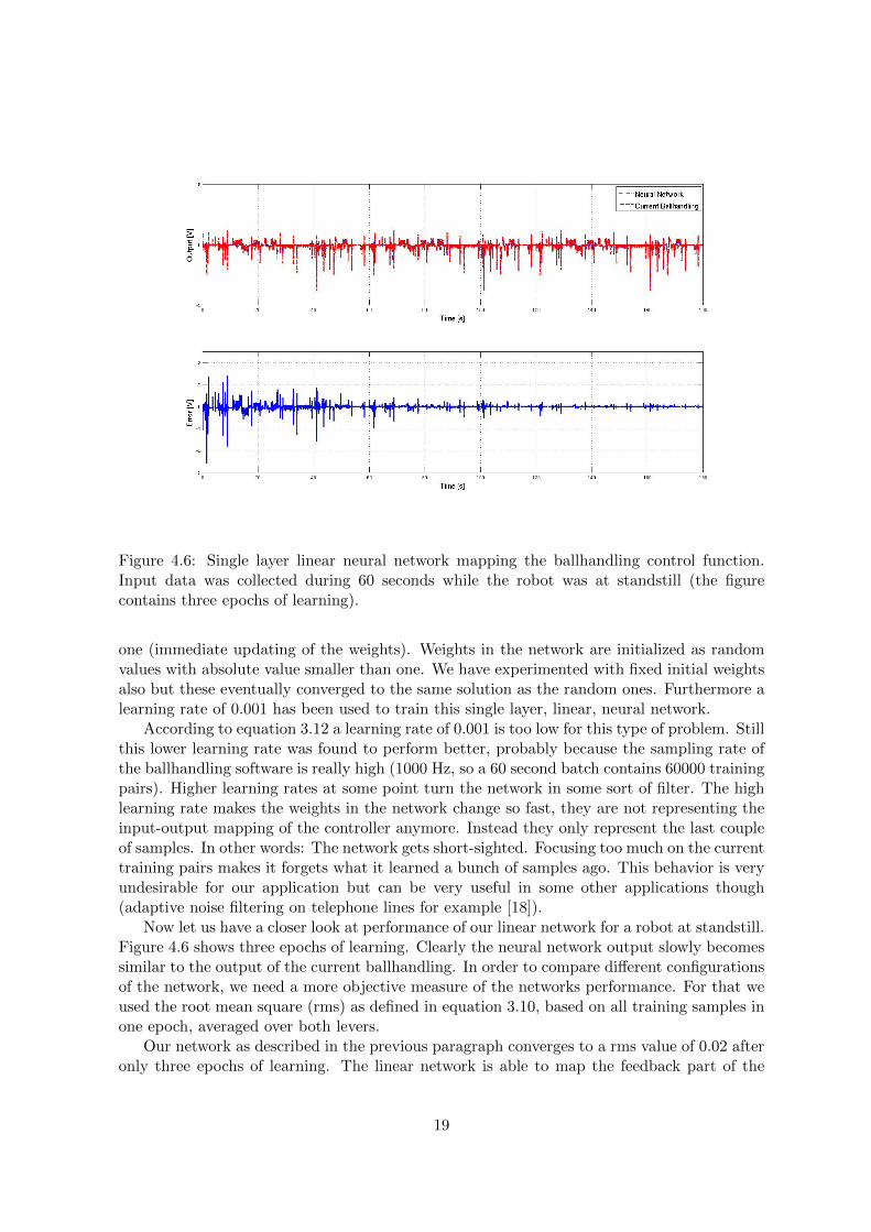
Figure 4.6: Single layer linear neural network mapping the ballhandling control function.Input data was collected during 60 seconds while the robot was at standstill (the figurecontains three epochs of learning).

one (immediate updating of the weights). Weights in the network are initialized as randomvalues with absolute value smaller than one. We have experimented with fixed initial weightsalso but these eventually converged to the same solution as the random ones. Furthermore alearning rate of 0.001 has been used to train this single layer, linear, neural network.

According to equation 3.12 a learning rate of 0.001 is too low for this type of problem. Stillthis lower learning rate was found to perform better, probably because the sampling rate ofthe ballhandling software is really high (1000 Hz, so a 60 second batch contains 60000 trainingpairs). Higher learning rates at some point turn the network in some sort of filter. The highlearning rate makes the weights in the network change so fast, they are not representing theinput-output mapping of the controller anymore. Instead they only represent the last coupleof samples. In other words: The network gets short-sighted. Focusing too much on the currenttraining pairs makes it forgets what it learned a bunch of samples ago. This behavior is veryundesirable for our application but can be very useful in some other applications though(adaptive noise filtering on telephone lines for example [18]).

Now let us have a closer look at performance of our linear network for a robot at standstill.Figure 4.6 shows three epochs of learning. Clearly the neural network output slowly becomessimilar to the output of the current ballhandling. In order to compare different configurationsof the network, we need a more objective measure of the networks performance. For that weused the root mean square (rms) as defined in equation 3.10, based on all training samples inone epoch, averaged over both levers.

Our network as described in the previous paragraph converges to a rms value of 0.02 afteronly three epochs of learning. The linear network is able to map the feedback part of the

19

Figure 4.7: Weights during three epochs of training data. The robot was not moving and wewere using a single layer, linear, neural network.

current ballhandling controller almost perfectly, which is not that surprising since this partof the controller involves only linear operations.

Figure 4.7 shows all eight weights present within the network, during the same timeinterval we discussed above. Because of the random initialization the beginning of the graphlooks messy but even though solutions to these mapping problems do not necessarily have tobe unique, all weights for the left and right lever converge to the same value.

For comparison we also conducted experiments providing the network with the filteredballhandling lever angles instead of the reference velocity from feedback (Fig. 4.3). Clearlythis led to a less perfect mapping. After three epochs of learning the network converged toa rms value of 0.12. The ballhandling control signal ranges between -1.5 and 1, which meansthe network on average still is about 5 percent off for each individual lever after being trainedwith this raw data. Providing the raw, unfiltered, data as input to the neural network wouldprobably lead to mappings that are even worse.

4.2 Robot moving around

Making the robot drive around while controlling the ball makes the mapping problem a lotmore challenging for our neural network. We will need more inputs but also the networkneeds to cover the non-linear transformations that are executed in the feedforward part ofthe current ballhandling controller (Fig. 4.3).

Logging data for a soccer robot that is moving around is not as straightforward comparedto logging data for a robot at standstill. It is better not to use a joystick to force the robotto drive in a certain direction because the feedforward input during manual control mode is

20

different from the input while the robot is moving autonomously. In joystick mode the robotuses the derivative of the encoder values measured at the omniwheels. During autonomousmode the robot uses the desired velocity that is calculated in the path planning part of thesoftware as input to the feedforward part of the controller.

We want disturbances and movement to resemble actual in-game situations as much aspossible. But putting a soccer robot in attacker mode would disturb the dataset with a lotof shooting interruptions. The dataset we are going to use within this section was gatheredby slightly adjusting the role of attacker main.2 Instead of searching for a good position toaim for a shot, the robot was instructed to drive randomly to any of the four corners of thefield (appendix B contains code to make the robot do so). Some noise was added to the exactposition of each of the corners such that different disturbances, caused by the field surface forexample, are applied.

4.2.1 Linear Network

Using a linear, single layer neural network with the same system parameters we used for therobot at standstill (zero bias value, learning rate of 0.001, random initial values) seemed towork perfectly. After only three epochs of learning the rms value reached 0.02. But inspectionof the error values showed the error only was decreasing during the first twenty percent ofthe first epoch.

By putting the learning rate to zero after the third epoch we discovered we were actuallylooking at the same short-sighted behavior described halfway section 4.1. This time loweringthe learning rate did not yield its desired effect. Lowering the learning rate as far as 10−7

the network was not short-sighted anymore, but since the root mean square for the convergednetwork equals 1.4 we can hardly speak of a mapping that makes sense. The linear networkcould be stuck in some local optimum but probably this type of network simply does not haveenough representational freedom to map the function we are looking for.

So the single layer linear network is not suited to imitate behavior of the current ballhan-dling controller. What about a multilayer linear neural network? Adding layers increases therepresentational power of a neural network so it probably is worthwhile to do some tests witha multilayer network.

Starting off with 1200 hidden layer elements (as advised by 3.11), random initial valuesas in the previous cases and α = 0.001 the network turned out to be unstable. Lowering thelearning rate made the network stable again but we could not get rid of the short sightedbehavior encountered before. Lowering the learning rate to 0.0000001 finally led to a rms of0.68. It took the network 37 epochs of learning to converge but when the learning rate wasput to zero after these 37 epochs, the rms immediately popped to 2.8. Again the network wasshort sighted, it only memorized the part of the function it saw most recent. Increasing thenumber of hidden layer elements did not help. Using 2500 hidden layer elements the networkended up with rms value equal to 0.91 after 35 epochs of learning but again the short-sightedbehavior occurred.

The short-sighted behavior we encountered so often now got us worried, especially becausethe amount of hidden layer elements (and thereby the representational power of the network)did not influence whether the phenomenon occurred or not. Are we asking the network to

2Tech Uniteds wiki page www.techunited.nl/wiki, together with recent Team Discription Papers http:

//www.techunited.nl/en/TDPs_MSL provide more info on how different roles are implemented to make therobots play soccer as a team.

21

www.techunited.nl/wiki

http://www.techunited.nl/en/TDPs_MSL

http://www.techunited.nl/en/TDPs_MSL

Figure 4.8: Multilayer linear neural network. Circles represent rms value after one epoch,blue line shows decreasing learning rate according to equation 4.1.

map a function it cannot represent, or are we asking the network to do the wrong thing inthe first place?

For the multilayer linear network, we considered the network to be converged once twosubsequent epochs’ rms value does not differ more than 0.05. Each update of the networkcauses the error to decrease, so a decrease of the root mean squared error over the entireepoch should imply we are looking at a better mapping of the function. But that is not truefor the ’short-sighted’ network configurations. Somehow they seem to be able to find a way tominimize rms without forcing the weights of the network to represent the function it is oughtto map. Instead of creating a set of weights that represents the function we are looking for,they learn how to optimally make use of the networks own learning abilities, the ability toadjust weights while moving through the epoch gets incorporated in the values of the weight.To overcome this behavior we should slowly decrease the learning rate during learning, forcingthe network to take a stance for the entire epoch.

After some initial tests, we decided to use annealing (Eq. 4.1), with t representing thediscretized learning time (over the entire trial, not just for the current epoch) and τ beinga constant value that fixes how fast the learning rate is decreasing. Manual tuning of thelearning rate led us to α = 0.000005 and τ = 18000. Figure 4.8 depicts the decreasinglearning rate together with rms values averaged over a single epoch. The net converges torms approximately equal to 3.5, which of course is not a proper mapping of the ballhandlingfunction but at least the network stores information, it is not short-sighted anymore.

α =α0

1 + tτ

(4.1)

22

4.2.2 Non-linear Network

Learning weights for a non-linear neural network took a lot more epochs compared to thelinear ones we have seen. After over a hundred epochs learning still was far from over so usingthe Simulink S-function structure we did in the previous subsection got a little inconvenient.Instead we used the m-file shown in appendix C.3. In order to decrease training time alsoa fixed number of training pairs was skipped after each step. Data was logged at 1000 Hzinitially, we decided to use only one out of 100 data points (which corresponds to one trainingpair per 0.1 seconds real-time).

First observation we made while training the non-linear network was that activation func-tions in the output layer were not necessary. In fact they were slowing down the learningprocess. Because we are using the tanh activation function, which has a maximum value ofone, non-linear nodes in the output layer cause the need to rescale the output. Omittingthe tanh here does not disturb learning, the loss in representational power can be coveredby adding a couple of hidden layer element. Without the non-linearity in output nodes theupdate rule both for weights between hidden layer and output layer 3.7 and for weights be-tween the input layer and hidden layer 3.9, needs to be slightly adapted. In both equations1 − tanh2(yink ) can be removed.

The second observation we made had to do with network settings. Decreasing the ’resolu-tion’ of training pairs from 1000 per second of logged data to 10 per second, largely influencedthe network settings that were found to be optimal. Optimal settings for α and the amount ofhidden layer units got really close to equations 3.12 and 3.11. Manually tuning resulted in thefollowing settings: Zero bias, 100 hidden layer elements with non-linear activation function,annealing learning rate as in Eq. 4.1 with α0 = 0.001 but t being the current epoch andτ = 500.

As said before, compared to the linear case, learning took a lot longer but results werealso much better. Convergence was defined as having two subsequent learning epochs whoserms values do not differ more than 10−5. Using this definition it took the network 1585epochs to converge. The root mean square over this final epoch was 0.099 (Fig. 4.9). Sinceannealing was used, the learning rate applied to this last epoch was decreased to 0.00024,approximately one third of the learning rate for the first epoch. As expected, the non-linearnetwork performs much better compared to the multilayer linear one.

Decreasing the resolution of training samples and longer learning increases the risk ofovertraining the network. In order to rule out this possibility the converged network has beentested on a couple of validation datasets. Depending on which part of the logged data wewere using, the rms for this validation set ranged between 0.1 and 0.98.

Violating the validation test for some of the sets was not caused by the network beingovertrained. Probably this latter set (with rms 0.98) covered part of the input space thatwas not part of the training batch. Figure 4.10 depicts the velocities in x, y and θ of therobot during the sixty seconds for which the logged data was used to train our network. Itinvolves sharp turns in many directions but it is not hard to imagine there can be certainmoves (input vectors) that are not incorporated in the data. Training the network on abigger dataset, containing all input vectors that occur during normal game-play might leadto a mapping that does well on all validation sets.

So the network is not overtrained. Inspecting the time domain plot of the learned network(Fig. 4.11) actually shows the opposite! The control signal by the neural network functionis more smooth than the original. Whether this indeed leads to better control of the ball is

23

Figure 4.9: Root mean square decreasing while mapping the ballhandling control function ofa moving robot with a non-linear neural net with 100 hidden layer elements.

Figure 4.10: Robot velocity during 60 seconds in forward, sideways and rotational direction(while logging data that was used to train the non-linear network with 100 hidden layerelements).

24

Figure 4.11: Control signal of the current ballhandling (blue) compared to the control signalprovided by the converged non-linear neural network (red), during 60 seconds.

investigated in the next section.

4.3 Real-time implementation

Three different executables are build and copied to the robot in order to make it play soccer:Vision, Worldmodel and Motion. This latter one takes care of control tasks but also containsstrategy and path planning software. Ballhandling is a low level control task so the neuralnetwork software will be implemented in the control scheme. Appendix D describes how todo so. In the remainder of this section results are discussed briefly.

As a first step the linear single layer network for a non-moving robot was implemented.Training the network off-line (section 4.1), we were able to make it converge to a reasonablerms value within three epochs of 60000 training pairs. In real time this would correspond tothree minutes of learning, which is acceptable. During tests this expectation was validated.Within a couple of minutes the robot was able to keep the ball at its reference position, despitedisturbances. When pushing the robot around the ball was eventually lost though. Feedbackalone clearly is not enough to make the robot properly control the ball, implementing thefeedforward loop is essential.

Off-line it took well over 1500 epochs to make the non-linear network imitate both thefeedforward and the feedback loop of the current ballhandling controller. Each epoch corre-sponded to sixty seconds of data logging so in real time it would take the network about 25hours to achieve the same degree of performance. During these hours the robot should haveto make exactly the same move over and over again. In practice it does not make sense toask someone to stay with the robot for this many hours. Hardware would suffer and most

25

people consider replacing batteries four times an hour a tedious job. But as explained inour problem statement, we would like to use the weights that were learned off-line as initialvalues for real-time learning. So let us have a look at real-time performance of the weightswe obtained in subsection 4.2.2.

After exporting the weights from Matlab workspace to C code, again the robot was putin ’four corners mode’. At first it seemed to do an awful job. The robot did not lose the ballbut while driving straight forward its ballhandling wheels were not spinning, it was simplypushing the ball around. Looking more closely we discovered that, even though drivingstraight forward was terrible, some of the other moves were executed perfectly. Turningaround its left axis, at a fixed position, or while slightly driving backwards, worked perfectly.Probably these were the moves that were incorporated in the dataset we were using to trainthe network.

Inspecting figure 4.10 tells us the robot was driving straight forward after approximatelyten seconds in the data set, but we cannot be sure anymore whether it was moving with orwithout ball. Therefore we conclude that at least some of the moves made by the robot duringlogging were successfully incorporated in the neural net. In the next chapter we elaborate,among others, on ways to incorporate all possible moves in the neural net.

26

Chapter 5

Future work

Now that we have validated the non-linear network is able to copy at least part of the ballhan-dling control function, we can think of ways to incorporate the entire input-output mappingof the ballhandling controller. One possible method would be to isolate the current controllerfrom the rest of the software. For each input an interval could be determined such that wecan generate random input vectors, observe their corresponding target vector and use themto obtain an infinitely long dataset of training pairs. A drawback of this method is that themapping will be equally good for every possible input vector. Forcing the network to performequally well within regions of input space that are rarely visited, could come at the cost ofnetwork performance within more important parts of input space.

Trying to improve learning speed for the non-linear network could be another interestingtopic for future research. The use of momentum methods and also the effect of additionalhidden layers could be studied. It would also be interesting to see whether a recurrent net isindeed able to map the entire ballhandling function, lowpass filters included (Fig. 4.3).

The topics suggested above assume the neural network should be implemented being thecontroller itself. This assumption implies, in order to meet our two goals stated in chapter 2,we need to find a way to replace the target vector with some other measured value representingnetwork performance. Doing so at every discretized step in time is very difficult. At the endof the day, performance of the network should be judged by whether or not the robot is ableto move around with the ball without ’pushing’ it. But once the robot loses possession ofthe ball, probably that is not because of a wrong signal exactly at the instant of time wherethe ball is lost. The output signal that needs to be updated might be generated hundredsof samples back in time. In machine learning literature this phenomenon is referred to as’delayed-reward’ (or punishment in this case, which is nothing but a negative reward).

Section 5.2 discusses Neural Fitted Q-iteration (NFQ), which is able to deal with theproblem of delayed-reward. Within a NFQ framework the neural network is used as a toolwithin a larger framework. It probably is more interesting for future work to study these typeof algorithms, instead of the ones where the neural net is implemented being the controlleritself. In order to meet control requirements, the neural control algorithm should be fastenough to operate in real-time, but moreover stability of the network should always be guar-anteed. Compared to most other control methods, stability properties for neural networksare ill-defined. It is hard to find comprehensive math that predicts exactly when the networkbecomes unstable, given its settings.

What is really impressive though, is the ability neural networks possess to map almost

27

any function imaginable. In the next section suggestions are made to use this enormousrepresentational power for system identification.

5.1 Neural system identification

Instead of trying to generate a mapping of a control function, neural networks can also be usedto automatically create a model of the plant. One of the methods to do so, is implementinga NARMAX network [10]. It involves a recurrent neural network, running in parallel to aplant and its controller. Inputs of this network at each step in time are the control inputs,the control signal corresponding to this input, but also previous control signals. Based onthat information the network tries to predict the state of the system at the next discrete stepin time. In fact, system identification is turned into supervisory learning.

In order to obtain a comprehensive neural predictor, we could choose to add noise to thecontrol output (comparable to the way control engineers inject white noise to measure thetransfer function of a plant). The learned predictor could be used to implement predictivecontrol techniques, but it could also be used to learn a controller function off-line. Since aproper representation of the system is available, large numbers of learning iterations are notproblematic anymore.

In the early nineties, the well-known ’truck backer-upper problem’ was solved using moreor less the same approach (chapter 12 in [11]). At first a neural network was trained to predictwhat short-term results of certain steering actions were (called the ’emulator’), hereafter thisemulator was used as a basis to learn a neural controller. For our ballhandling system asimilar approach could be interesting.

5.2 Neural Fitted Q-Iteration

Q-iteration is a widely used form of reinforcement learning. The concept has been usedto learn high level team strategies within the RoboCup soccer simulation league ([15], [9]and [14]), but also for low-level motor control within the middle size league [8]. In 2008the Brainstormers Tribots team revealed their robot was able to real-time learn reasonabledribbling behavior within minutes [5].

An extensive introduction to reinforcement learning is given by [16], below some thoughtson the possible role of a neural network within reinforcement learning for ballhandling willbe shared. Three basic building blocks form a base for any reinforcement learning algorithm:Rewards, States and Actions.

In Q-learning a value is stored for each unique state-action pair (s, a). By allowing theagent to interact with its environment, eventually these Q-values represent the amount offuture reward the agent is expected to receive after taking action a out of state s.

In order to apply this framework to our ballhandling task, we have to make choices onhow to evaluate reward at each state. We should keep in mind the reward signal is only meantto tell the learning agent what its goal should be, not how to reach it. Therefore a suitablechoice could be to distribute a large negative reward every time the robot loses the ball (butnot during a shot or while passing the ball to a teammate).

State and action space in ballhandling are continuous, so we should somehow discretizethese signals in order to be able to store a Q-value for each state-action pair experienced bythe robot. For action space we can simply choose to use five possible output voltages. In case

28

the robot does not have enough freedom choosing out of these five actions, the number can beincreased but we should try to keep it low as possible though. The total amount of Q-valueswill be equal to all possible states multiplied by the number of possible actions. Learningtime is largely determined by the amount of Q-values to be learned, so we should keep thisamount low as possible.

Discretization of state space is a little more complicated, compared to action space. Usu-ally people choose to simply cut the range of each entry in the state vector in, for example, tenpieces. One such piece is called a ’feature’. For each continuous state input, we can determinethe features that are present. The discretized state than consists of a vector containing foreach state entry the identifier of the feature that is currently present there. This method iscalled linear tile coding.

For ballhandling we used seven inputs, suppose we indeed discretize these using ten fea-tures for each state, and suppose we indeed use an action space containing five possibleactions, the amount of Q-values to be learned would then be equal to 5 · 107 = 50000000. Itwould take way too long to learn an amount of Q-values this big. This phenomenon is called’the curse of dimensionality’ and it is here that the neural network could step in.

Instead of chopping state inputs into features, we could simply use the continuous statesignal and provide it to a neural network similar to the one we used to map our ballhandlingcontroller. The output of this neural network will be our Q-value. Using the update rulefor Q-values, we can obtain the error that can be used to train the neural network, forcingit to converge to a Q-value that properly represents the amount of future reward for thecorresponding state-action pair. The mapping from continuous state input to Q-value cantake any arbitrary form and will be highly non-linear. As said before, neural networks arevery well suited to find these mappings.

Generalization between different state variables is the reason both tile coding and neuralnetworks can cope with the curse of dimensionality. A learned experienced will change thevalue of the corresponding Q-value, but it will also change the Q-value in regions of state spacethat are only partly coinciding with the current state. Generalization speeds up learning, butat some point it could also destroy knowledge we have of one particular part in state spaceso far (with updates resulting from another region).

In [12] a NFQ method is presented that uses batch updating. By logging the entirebatch of state-action transitions, the neural network can be fitted off-line, using the entireepoch of learning experiences. This batch updating method prevents the erase of properQ-values learned earlier, because the network is always fitted through the entire batch. TheBrainstormers Tribots team has used batch updated NFQ to automatically create a ball-pushing strategy (without active control of ballhandling wheels) [13]. Incorporating our activeballhandling mechanism within their work would by an extremely interesting topic for futureresearch.

29

Chapter 6

Conclusion

Our initial goal of creating a learning algorithm that outperforms the current ballhandlingturned out to be a little too ambitious for this assignment. One reason we were not yet able tocreate a self-learning ballhandling controller, was the large amount of time spent on practicalissues (writing code to make the robots drive around in a random pattern, learning how tolog data, how to write Matlab S-Functions etc). In the appendices of this report these topicsare carefully documented, which hopefully saves future students studying the ballhandlingsoftware a lot of time.

Another cause of delay was the large amount of time spend on manually tuning thelearning parameters of the neural networks we investigated. Math that exactly prescribeswhich settings (number of hidden layer elements, learning rate) are optimal was not foundso these settings had to be tuned by hand. One of the reasons to study neural networks forballhandling control, was the reduced need to regularly tune the system. It is questionablewhether a neural net indeed would save us time here. We might be ’filling one hole withanother’, which is a Dutch expression people use for someone who lends money to pay debt.Instead of tuning the parameters of the previous controller, we are now tuning parameters ofthe neural network.

Our other reason to study this topic was the ability of neural nets to map highly non-linearfunctions. These capabilities indeed were promising but in order to use them in a controllerthat performs better than the current one, a bigger framework is needed. The chapter onfuture work briefly describes two ways to get to a unsupervised learning framework. Eitherthe neural network could be used for system identification, which provides us with a modelof the system that could be used to learn a controller off-line, or the neural network could beused within a neural fitted Q-iteration environment, which allows the robot to learn real-time.This latter method has proven to work for ball pushing strategies at other teams.

Even though we did not reach our final goal of self-learning ballhandling control, thisassignment has been really useful. Implementing the network directly on a real life experi-mental setup requires a much deeper understanding of the learning algorithm (compared tosimulated experiments). Closely inspecting the input data led to a better understanding offunctions feedforward neural networks can or cannot map. Multilayer feedforward networksare often used in a lot of different environments. Knowledge gained during this assignmenttherefore is useful in a wide range of applications.

In his book chapter ’Connectionist Learning for Control’, published in 1991, Andrew G.Barto discusses the interface between traditional, math based, control science and the more

30

AI based heuristic approach (page nine of [11]). He saw this field of science as if ’scientistsfrom different but similar planets suddenly found themselves able to communicate’, which ledto ’a sudden flow of information as concepts on each side are recast within the other sidesframeworks’. In the past twenty years bridging the gap described by Barto resulted in manyimpressive examples of learning control. Our ballhandling mechanism will follow soon.

31

Bibliography

[1] Bram Bakker. The State of Mind - Reinforcement Learning with Recurrent Neural Net-works. 2004.

[2] J.J.T.H. de Best, M.J.G. van de Molengraft, and M. Steinbuch. A novel ball handlingmechanism for the robocup middle size league. IFAC Mechatronics, 2010. http://goo.gl/a82oo.

[3] L. Appeltant et. al. Information processing using a single dynamical node as complexsystem. Nat. Commun. 2:468, 2011.

[4] F.M.W. Kanters et.al. Tech united eindhoven team description 2011. Team descriptionpaper RoboCup middle size league, 2011. http://goo.gl/ySXTF.

[5] Roland Hafner et.al. Brianstormers tribots team description. 2008.

[6] L. Fausett. Fundamentals of Neural Networks - Architectures, Algorithms and Applica-tions. 1994.

[7] Bill Gates. A robot in every home - the leader of the pc revolution predicts that the nexthot field will be robotics. Scientific American, INC, 2006.

[8] Roland Hafner and Martin Riedmiller. Neural reinforcement learning controllers for areal robot application. year unknown.

[9] Shivaram Kalyanakrishnan, Yaxin Liu, and Peter Stone. Half field offense in robocupsoccer: A multiagent reinforcement learning case study. 2006.

[10] Mircea Lazar and Octavian Pastravanu. A neural predictive controller for non-linearsystems. Elsevier, Mathematics and Computers in Simulation, 2002.

[11] Thomas Miller, Richard Sutton, and Paul Werbos. Neural Networks for Control. 1991.

[12] Martin Riedmiller. Neural fitted q iteration - first experiences with a data efficient neuralreinforcement learning method. Springer-Verlag Berlin Heidelberg, 2005.

[13] Martin Riedmiller, Thomas Gabel, Roland Hafner, and Sascha Lange. Reinforcementlearning for robot soccer. Auton Robot, 2009.

[14] Robin Soetens. Reinforcement learning applied to keepaway, a robocup soccer subtask,2010. Bachelor Final Project http://goo.gl/oL7dJ.

32

http://goo.gl/a82oo

http://goo.gl/a82oo

http://goo.gl/ySXTF

http://goo.gl/oL7dJ

[15] Peter Stone, Richard Sutton, and Gregory Kuhlman. Reinforcement learning for robocupsoccer keepaway. 2005.

[16] Richard S. Sutton and Andrew G. Barto. Reinforcement Learning, an Introduction. 1998.

[17] V.N. Vapnik. An overview of statistical learning theory. IEEE Transactions on NeuralNetworks, VOL. 10, NO. 5, 1999.

[18] Bernard Widrow and Rodney Winter. Neural nets for adaptive filtering and adaptivepattern recognition. IEEE, 1988.

33

Appendix A

List of symbols used in text

Symbol Unit Explanation

xrobot m/s velocity x direction robot (straight forward)yrobot m/s velocity y direction robot (sideways)

θrobot rad/s angular velocity robot (vertical axis)φlever rad position ballhandling lever (either left or right)φll rad position left ballhandling leverφrl rad position right ballhandling lever

φball rad/s angular velocity ballhandling wheel (either left or right)

φlb rad/s angular velocity left ballhandling wheel

φrb rad/s angular velocity right ballhandling wheelx - vector containing input values neural network (including bias)z - vector containing values at hidden layer neural networkzinj - value at hidden node j after summation but before activation function

y - vector containing output values neural networkvij - weight between input node i and hidden node jwjk - weight between hidden node j and output node kV - matrix of weights between input layer and hidden layerW - matrix of weights between hidden layer and the output layerα - learning rate 0 < α < 1T - size of training set (number of training vectors)H - number of nodes in hidden layerM - number of outputsN - number of inputsα0 - initial learning rate during annealingt - discretized time during learning (counts number of training pairs passed)τ - fixes decay of learning rate during annealings - state, within a reinforcement learning frameworka - action, within a reinforcement learning framework

34

Appendix B

Logging data

Methods to log data presented in this appendix are tested for Tech United MSL SVN version4277. Code was build using Matlab version R2007b with Ubuntu 8.10. A compressed folderwith all code, logged data and figures used in this report, can be obtained here: goo.gl/pf9i0

The folder ’data logging’ contains a file ’ballhandling.c’, replace the file that is currentlyin ../Motion/src with this one, than make and build the software in order to log data. Thematfile you will obtain1 is logged at 1000 Hz where each row consists of one ’logvector’:

logvector[0] = uBH[0];

logvector[1] = uBH[1];

logvector[2] = psfgd->tachoFilt[0];

logvector[3] = psfgd->tachoFilt[1];

logvector[4] = psfgd->rBHPosFilt[0];

logvector[5] = psfgd->rBHPosFilt[1];

logvector[6] = pmotionbus->velLocalRef_dxdydo[0];



logvector[9] = *CPBrobot;

logvector[10] = psfgd->BHAngleFilt[0];

logvector[11] = psfgd->BHAngleFilt[1];

logvector[12] = addEffBH[0];

logvector[13] = addEffBH[1];

logvector[14] = *retractBall;

The script ’reshape BH data.m’ can be used to convert the matfile to a format thatis accepted either by the s-function neural network of appendix C.1 or the m-file shown inappendix C.3. In order to use use the logged data within the separate C executable (AppendixC.2), a Simulink model called ’convertmatfile2logfile’ can be used.

1A script called ’copysimoutdatafromturtle turtlex’ can be used to download data from the robot via a wificonnection. http://goo.gl/ipPYg

35

goo.gl/pf9i0

http://goo.gl/ipPYg

B.1 Robot at standstill

BH standstill turtle4.mat contains over one minute of logged ballhandling data, during log-ging the robot did not move but disturbances to the ballhandling were supplied manually(pulling the ball out, pushing it left and right etc).

B.2 Moving robot

BH moving turtle4.mat contains about one and a half minute of data that was logged whilethe robot was put in a ’four corners pattern’, driving randomly from corner to corner whilecontrolling the ball. In order to make the robot do so, either follow instructions bellow orreplace the files in ../Motion/src with the ones provided with this report.Replace function ’Advanced Attack’ in ’role attacker main.c’ with:

/* Orientation: orientation of the robot during the attack,

* 0: forward attack

* M_PI: backward attack */

/* global data */

psfun_global_data psfgd;

pdyn_pass_data pdpd;

get_pointers_to_global_data2(&psfgd, &pdpd, S);

int i;

int n_targets;

n_targets = 2; /* only x,y (no rotation) */

int four_corners;

int reached_position;

double distance_togo;

double Turtle_Target[n_targets];

reached_position = 1;

/* shorter writing */

double FW = FIELDWIDTH;

double FL = FIELDLENGTH;

/* choose between four noisy corners pattern and fully random */

four_corners = 0;

for( i = 0 ; i < n_targets ; ++i ){

distance_togo = abs(pS_in->cur_xyo[i]-psfgd->prev_Turtle_Target[i]);

if( distance_togo > 1 ){

reached_position = 0;

}

36

}

if( reached_position ){

if( four_corners ){

int corner = rand() % 4;

double corners_x[4] = { 0.4*FW, -0.4*FW, 0.4*FW, -0.4*FW };

double corners_y[4] = { 0.4*FL, -0.4*FL, -0.4*FL, 0.4*FL };

Turtle_Target[0] = corners_x[corner]+(rand()%20)/10.0-0.95;

Turtle_Target[1] = corners_y[corner]+(rand()%20)/10.0-0.95;

}

else {

Turtle_Target[0] = (rand()%200-99.5)/100.0*0.5*(FW-0.5);

Turtle_Target[1] = (rand()%200-99.5)/100.0*0.5*(FL-0.5);

}


psfgd->prev_Turtle_Target[i] = Turtle_Target[i];

}

}

else {


Turtle_Target[i] = psfgd->prev_Turtle_Target[i];

}

}

DoAction(Action_DribbleToTarget, pS_AHP, Turtle_Target);

Append to global data in rolehandler.h:

/* for random driving (logging data for NN) */

double prev_Turtle_Target[2];

Add to mdlInitializeConditions of rolehandler.c:

/* for random driving (logging data for NN) */

for( i = 0 ; i < 2 ; ++i ) {

psfgd->prev_Turtle_Target[i] = 0.0;

}

37

Appendix C

Neural network code, threedifferent implementations

The code below (except for the separate C executable) have been tested using Ubuntu 8.10as an operating system and Matlab version R2007b. The Standalone executable presented insection C.2 was compiled using Gnu C Compiler (gcc) version 4.6.1 with operating systemUbuntu 11.10

A compressed folder with all code, logged data and figures used in this report, can bedownloaded here: http://goo.gl/pf9i0

C.1 Simulink S-function

BH NN LIN.h

/* Ballhandling using Neural Network */

/* Gerrit Naus and Robin Soetens */

/* January 2012 */

#ifndef _LIN_NN_

#define _LIN_NN_

#define INPUTS_NN 5

#define OUTPUTS_NN 2

/* define global data struct */

typedef struct tag_sfun_global_data {

/* weights linear single layer neural network */

double NN_Weights[OUTPUTS_NN][INPUTS_NN];

/* cummulative weight updates, for batch updating */

double NN_Weights_update[OUTPUTS_NN][INPUTS_NN];

/* counts number of evaluated training pairs */

int stepcount;

38

http://goo.gl/pf9i0

/* cummulative error for current epoch */

double total_err;

} sfun_global_data, *psfun_global_data;

#endif

BH NN LIN.c

/* Ballhandling using Neural Network */

/* Gerrit Naus and Robin Soetens */

/* January 2012 */

#define S_FUNCTION_NAME BH_NN_LIN

#define S_FUNCTION_LEVEL 2

/* include h-files */

#include <time.h>

#include <stdio.h>

#include <stdlib.h>

#include <math.h>

#include "simstruc.h"

#include "BH_NN_LIN.h"

/*******************************

* Input Ports definitions *

*******************************/

#define NINPUTS 6 /* number of input ports (0...)*/

#define NINPUTS0 1 /* velocity reference left lever */

#define NINPUTS1 1 /* velocity reference right lever */

#define NINPUTS2 1 /* tacho measured velocity left wheel */

#define NINPUTS3 1 /* tacho measured velocity right wheel */

#define NINPUTS4 1 /* target JdB controller left wheel */

#define NINPUTS5 1 /* target JdB controller right wheel */

#define NPARAMS 0

int INPUT_DEF[ NINPUTS ] = { NINPUTS0, NINPUTS1, NINPUTS2, NINPUTS3, . . .

NINPUTS4, NINPUTS5 };

/********************************

* Output Ports definitions *

********************************/

#define NOUTPUTS 6 /* number of output ports (0...) */

#define NOUTPUTS0 1 /* velocity left wheel NN */

#define NOUTPUTS1 1 /* velocity right wheel NN */

39

#define NOUTPUTS2 2 /* error, left and right */

#define NOUTPUTS3 1 /* rms of error, sum of both levers */

#define NOUTPUTS4 5 /* weights providing output left wheel */

#define NOUTPUTS5 5 /* weights providing output right wheel */

int OUTPUT_DEF[ NOUTPUTS ] = { NOUTPUTS0, NOUTPUTS1, NOUTPUTS2, . . .

NOUTPUTS3, NOUTPUTS4, NOUTPUTS5 };

/*************************************************************************/

static void mdlInitializeSizes(SimStruct *S)

{

int_T Rworksize;

ssSetNumSFcnParams(S, NPARAMS);

if (ssGetNumSFcnParams(S) != ssGetSFcnParamsCount(S)) {

return;

}

/***************************

* Input Ports definitions *

***************************/

if (!ssSetNumInputPorts(S,NINPUTS)) return;

int i;

for(i=0;i<NINPUTS;++i){

ssSetInputPortWidth(S,i,INPUT_DEF[i]);

ssSetInputPortDataType(S,i,SS_DOUBLE);

ssSetInputPortDirectFeedThrough(S,i,1);

ssSetInputPortRequiredContiguous(S,i,1);

}

/****************************

* Output Ports definitions *

****************************/

if (!ssSetNumOutputPorts(S,NOUTPUTS)) return;

for(i=0;i<NOUTPUTS;++i){

ssSetOutputPortWidth(S,i,OUTPUT_DEF[i]);

ssSetOutputPortDataType(S,i,SS_DOUBLE);

}

/***********************

* Definition of States *

************************/

ssSetNumContStates(S, 0);

ssSetNumDiscStates(S, 0);

40

/**********************

* Default Definitions *

**********************/

ssSetNumSampleTimes(S, 1);

/* compute necessary amount of real_T workspace */

Rworksize = ( sizeof(sfun_global_data)/sizeof(real_T) + 1 );

ssSetNumRWork(S, Rworksize);

ssSetNumIWork(S, 0);

ssSetNumPWork(S, 0);

ssSetNumModes(S, 0);

}

/*************************************************************************/

static void mdlInitializeSampleTimes(SimStruct *S)

{

ssSetSampleTime(S, 0, INHERITED_SAMPLE_TIME);

ssSetOffsetTime(S, 0, 0.0);

}

/*************************************************************************/

#define MDL_INITIALIZE_CONDITIONS

#if defined(MDL_INITIALIZE_CONDITIONS)

static void mdlInitializeConditions(SimStruct *S)

{

/* get pointers to global data */

real_T* ptrRwrk = ssGetRWork(S);


psfgd = (psfun_global_data) ptrRwrk;

/* init weights (global) */

int i,j;

for(i=0;i<OUTPUTS_NN;++i){

for(j=0;j<INPUTS_NN;++j){

psfgd->NN_Weights[i][j] = rand() % 101 / 100.0;

psfgd->NN_Weights_update[i][j] = 0.0;

}

}

psfgd->stepcount = 0;

}

#endif

41

/*************************************************************************/

static void mdlOutputs(SimStruct *S, int_T tid)

{

/* get pointers to global data */


real_T* pRwrk = ssGetRWork(S);

psfgd = (psfun_global_data) pRwrk;

/* parameters */

double lr = 0.001; /* learning rate */

double bias = 0.0; /* bias input NN */

int stop_learning_at = -1; /* training sample at which learning rate

is put to zero (submit -1 for never) */

int batch_length = 1; /* number of training pairs before update

(submit 1 for online learning) */

int epoch_size = 60000; /* number of training pairs in one epoch */

int i,j; /* counters */

/* stop learning after number of samples */

if ( psfgd->stepcount > stop_learning_at && stop_learning_at != -1 ){

lr = 0.0;

}

/* pointers to input ports */

double* arm_left = ( double *)ssGetInputPortSignal(S,0);

double* arm_right = ( double *)ssGetInputPortSignal(S,1);

double* tacho_left = ( double *)ssGetInputPortSignal(S,2);

double* tacho_right = ( double *)ssGetInputPortSignal(S,3);

double* ball_left = ( double *)ssGetInputPortSignal(S,4);

double* ball_right = ( double *)ssGetInputPortSignal(S,5);

/* pointers to output ports */

double* NN_ball_left = (double *)ssGetOutputPortSignal(S,0);

double* NN_ball_right = (double *)ssGetOutputPortSignal(S,1);

double* error_inscope = (double *)ssGetOutputPortSignal(S,2);

double* rms_out = (double*)ssGetOutputPortSignal(S,3);

double* weights_out_1 = (double*)ssGetOutputPortSignal(S,4);

double* weights_out_2 = (double*)ssGetOutputPortSignal(S,5);

double input[INPUTS_NN];

input[0] = bias;

input[1] = *arm_left;

input[2] = *arm_right;

input[3] = *tacho_left;

input[4] = *tacho_right;

42

double output[OUTPUTS_NN] = { 0.0 , 0.0 };

/* calculate output NN */



output[i] += psfgd->NN_Weights[i][j]*input[j];

}

}

*NN_ball_left = output[0];

*NN_ball_right = output[1];

double ball[2];

ball[0] = *ball_left;

ball[1] = *ball_right;

double error[2] = { ball[0]-output[0] , ball[1]-output[1] };

memcpy( error_inscope , &error , sizeof(error) );

/* update weights */



psfgd->NN_Weights_update[i][j]+=lr*(ball[i]-output[i])*input[j];

}

}

if( psfgd->stepcount % batch_length == 0 ){


for(j=0;j<INPUTS_NN;++j)

{

psfgd->NN_Weights[i][j] += psfgd->NN_Weights_update[i][j]/batch_length;


}

}

}

/* root mean squared for current epoch (average of both levers) */

double rms = 0.0;

if( (psfgd->stepcount % epoch_size ) == 0){

psfgd->total_err = 0.0;

}

psfgd->total_err += 0.5 * ( pow( error[0], 2) + pow( error[1], 2) );

rms = sqrt( psfgd->total_err / ( psfgd->stepcount % epoch_size + 1 ) );

43

*rms_out = rms;

/* show weights in scope */

double weights_out1[INPUTS_NN];

double weights_out2[INPUTS_NN];


weights_out1[j] = psfgd->NN_Weights[0][j];

weights_out2[j] = psfgd->NN_Weights[1][j];

}

memcpy( weights_out_1 , &weights_out1 , sizeof(weights_out1) );

memcpy( weights_out_2 , &weights_out2 , sizeof(weights_out2) );

psfgd->stepcount += 1;

}

/*************************************************************************/

static void mdlTerminate(SimStruct *S)

{

}

#ifdef MATLAB_MEX_FILE /* Is this file being compiled as a MEX-file? */

#include "simulink.c" /* MEX-file interface mechanism */

#else

#include "cg_sfun.h" /* Code generation registration function */

#endif

44

C.2 Standalone executable

BH NN NL FF.h

/* Robin Soetens, Ballhandling using Neural Network */

/* November 2011 */

#ifndef NN_BALHANDLING_

#define NN_BALHANDLING_

/* size of neural network */

#define InputsNN 6

#define HLE 100

#define OutputsNN 2

/* size of training set */

#define N_COLUMNS_LOGFILE 8

#define N_LINES_LOGFILE 70000

/* file management */

FILE* logfile_p;

char* data_str_p;

char dataline[ 40 * N_COLUMNS_LOGFILE ];

char logfile_dir[] = "SUBMIT DIR TO FILE!";

/* learning parameters */

double lr = 0.15;

double bias = 1.0;

double error_threshold = 0.001;

int skip_samples = 100;

/* weights matrix */

double BHNNW_V[HLE-1][InputsNN];

double BHNNW_W[OutputsNN][HLE];

/* input, output vectors */

double input[N_LINES_LOGFILE][InputsNN];

double y_out[N_LINES_LOGFILE][OutputsNN];

double y_in[OutputsNN];

double z_in[HLE-1];

double z_out[HLE];

double target[N_LINES_LOGFILE][OutputsNN];

double error[N_LINES_LOGFILE][OutputsNN];

int CPB[N_LINES_LOGFILE];

45

/* general parameters */

int stop;

/* functions */

void PrintParameters();

void InitializeWeights();

void InitializeTrainingSet();

void ResetParametersNN ( int n_iteration );

void OutputHiddenLayer( int n_iteration );

void OutputNN( int n_iteration );

void ErrorNN( int n_iteration );

void UpdateWeights( int n_iteration );

void EvaluateCurrentEpoch();

#endif

BH NN NL FF.c


/* November 2011 */

#include <time.h>

#include <stdio.h>

#include <stdlib.h>

#include <math.h>

#include "BH_NN_NL_FF.h"

#include "BH_NN_NL_FF_Functions.h"

int main ()

{

PrintParameters();

int n_iteration;

int n_epoch = 0;

/* initialization */

InitializeWeights();

InitializeTrainingSet();

stop = 0;

46

while(!stop)

{

n_iteration = 0;

printf("Epoch number %d starts\n", n_epoch );

for(n_iteration=0;n_iteration<N_LINES_LOGFILE;n_iteration+=skip_samples)

{

/* reset NN parameters */

ResetParametersNN( n_iteration );

/* calculate output hidden layer NN */

OutputHiddenLayer( n_iteration );


OutputNN( n_iteration );

/* obtain temporal error */

ErrorNN( n_iteration );


UpdateWeights( n_iteration );

/* store output NN */

if( n_iteration%10000 == 0 )

{

printf(".");

}

}

/* check stopping condition */

EvaluateCurrentEpoch();

++n_epoch;

}

return 0;

}

47

BH NN NL FF Functions.h


/* November 2011 */

#ifndef NN_BALHANDLING_FUNCTIONS_

#define NN_BALHANDLING_FUNCTIONS_

void PrintParameters()

{

printf("\n================================================ . . .

=============================================================== \ n");

printf("\n You’re about to witness a non-linear multilayer . . .

feedforward neural network in action \ n");

printf("\n Robin Soetens - November 2011 \n");

printf("\n Learning rate = %1.10f", lr);

printf("\n Rms error threshold = %1.10f", error_threshold);

printf("\n Number of hidden layer elements = %d \n", HLE);

printf("\n Using training set from: %-3.200s \n", logfile_dir );

printf("\n================================================ . . .

=============================================================== \ n \ n");

}

void InitializeWeights()

{

int i,j,k;


for( i = 0 ; i < InputsNN ; ++i ){

for( j = 0 ; j < HLE-1 ; ++j )

{

/* top layer */

BHNNW_V[j][i] = 1.0; rand() % 101 / 10.0 - 5.0;

}

}


for( k = 0 ; k < OutputsNN ; ++k ){

for( j = 0 ; j < HLE ; ++j )

{

/* hidden layer */

BHNNW_W[k][j] = 1.0; rand() % 101 / 100.0 - 5.0;

}

}

48

}

void InitializeTrainingSet()

{

double tempvect[ N_COLUMNS_LOGFILE ];

int i,j,k;

/* Look for initial values file */

logfile_p = fopen( logfile_dir , "r" );

if( logfile_p == NULL )

{

printf("Error: could not open logfile with training set!\n");

stop = 1;

}

for( i = 0 ; i < N_LINES_LOGFILE ; ++i )

{

/* Read line from logfile */

fgets( dataline, 35 * N_COLUMNS_LOGFILE , logfile_p );

j = 0;

data_str_p = strtok( dataline , "\t\t" );

while( data_str_p != NULL )

{

tempvect[j] = atof( data_str_p );

data_str_p = strtok( NULL , "\t" );

++j;

}

input[i][0] = bias;

input[i][1] = tempvect[0]; /* arm_left */

input[i][2] = tempvect[1]; /* arm_right */

input[i][3] = tempvect[4]; /* robot_x */

input[i][4] = tempvect[5]; /* robot_y */

input[i][5] = tempvect[6]; /* robot_spin */

target[i][0] = tempvect[2]; /* ball_left */

target[i][1] = tempvect[3]; /* ball_right */

CPB[i] = tempvect[7]; /* check possession ball */

}

fclose( logfile_p );

49

}

void ResetParametersNN (int n_iteration)

{

int i,j,k;

for( i = 0 ; i < OutputsNN ; ++i )

{

y_out[n_iteration][i] = 0.0;

y_in[i] = 0.0;

}

for( i = 0 ; i < HLE-1 ; ++i )

{

z_in[i] = 0.0;

z_out[i+1] = 0.0;

}

z_out[0] = bias;

}

void OutputHiddenLayer( int n_iteration )

{

int i,j,k;

for( j = 0 ; j < HLE-1 ; ++j )

{

for( i = 0 ; i < InputsNN ; ++i )

{

z_in[j] += BHNNW_V[j][i]*input[n_iteration][i];

z_out[j+1] += tanh ( z_in[j] );

}

}

}

void OutputNN( int n_iteration )

{

int i,j,k;

for( k = 0; k < OutputsNN; ++k )

{

for( j = 0 ; j < HLE ; ++j )

{

y_in[k] += BHNNW_W[k][j]*z_out[j];

y_out[n_iteration][k] += tanh( y_in[k] );

}

50

}

}

void ErrorNN( int n_iteration )

{

int i,j,k;


{

error[n_iteration][i] = target[n_iteration][i]-y_out[n_iteration][i];

}

}

void UpdateWeights( int n_iteration )

{

int i,j,k;

for( k = 0 ; k < OutputsNN ; ++k )

{

for( j = 0 ; j < HLE ; ++j )

{

BHNNW_W[k][j] += lr * error[n_iteration][k] * . . .

(1.0 - pow( tanh( y_in[k] ), 2 ) ) * z_out[j];

}

}

for( j = 0 ; j < HLE-1 ; ++j )

{

for( i = 0 ; i < InputsNN ; ++i )

{

for( k = 0 ; k < OutputsNN ; ++k )

{

BHNNW_V[j][i] += lr * error[n_iteration][k] * . . .

(1.0 - pow( tanh( y_in[k] ) , 2 ) ) * BHNNW_W[k][j] * . . .

(1.0 - pow( tanh( z_in[j] ) , 2 ) ) * input[n_iteration][i];

}

}

}

}

void EvaluateCurrentEpoch()

{

int i,j,k;

double rms_error = 0.0;


51

{

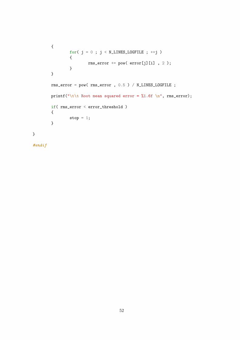
for( j = 0 ; j < N_LINES_LOGFILE ; ++j )

{

rms_error += pow( error[j][i] , 2 );

}

}

rms_error = pow( rms_error , 0.5 ) / N_LINES_LOGFILE ;

printf("\t\t Root mean squared error = %1.6f \n", rms_error);

if( rms_error < error_threshold )

{

stop = 1;

}

}

#endif

52

C.3 M-file implementation

%% Feedforward Neural Network mapping ballhandling control function

%

% Robin Soetens - January 2012

% Course on ’Non-linear systems and neural networks - 5P060’

%

clear all

close all

clc

nonlin = 1; % submit 1 for nonlinear tanh() activation function

n_hle = 100; % number of hidden layer elements, include bias, -1 for no hl

lr0 = 1e-3; % learning rate at first epoch

decr = 500; % increase to make lr decr slower, -1 for const, 0 for lin decay

bias = 0.0; % bias input

tol_conv = 0.00001; % convergence check

dec = 100; % skip amount of samples, submit 1 to not skip anny

it = 1; % indicates current training pair

stop = 0; % equal to 1 once net is converged, 2 for unstable net

epoch =1; % indicates current epoch

%% start loop over training epochs

while stop ~= 1 && stop ~= 2

%% load training pairs

load inputs.mat

load targets.mat

[ dummy1 , n_inputs ] = size( inputs );

[ dummy2 , n_outputs ] = size( targets );

n_inputs = n_inputs + 1;

if dummy1 ~= dummy2

error(’Number of input vectors does not correspond to . . .

number of target vectors!’)

else

total_size = dummy1;

clear dummy1 dummy2

end

if epoch == 1

disp(sprintf(’Training pairs loaded, . . .

53

total size = %d\n’,total_size))

end

% skip samples

epoch_size = total_size / dec;

if dec ==1

tr_inputs = inputs;

tr_targets = targets;

else

tr_inputs = zeros(epoch_size,n_inputs-1);

tr_targets = zeros(epoch_size,n_outputs);

j = 1;

for i = 1:dec:total_size

tr_inputs(j,:) = inputs(i,:);

tr_targets(j,:) = targets(i,:);

j = j + 1;

end

end

%% initialize weights

if epoch == 1;

if n_hle == -1

weights = rand(n_outputs, n_inputs);

else

weights_in = rand(n_hle, n_inputs);

weights_out = rand(n_outputs, n_hle);

end

disp(sprintf(’Weights initialized\n’))

end

error_nn = zeros(epoch_size,n_outputs);

output_nn = zeros(epoch_size,n_outputs);

%% start loop current epoch

for it = 1:epoch_size

% forward phase, calculate output neural network

input_nn = [ bias; tr_inputs(it,:)’ ];

if n_hle == -1

output_nn(it,:) = weights * input_nn;

else

output_hl_in = weights_in * input_nn;

if nonlin == 1

output_hl = tanh(output_hl_in);

else

output_hl = output_hl_in;

end

54

output_hl(1) = bias;

output_nn(it,:) = ( weights_out * output_hl )’;

end

% observe error, store to determine rms

error_nn(it,:) = tr_targets(it,:) - output_nn(it,:);

% backward phase, update weights

if decr == -1

lr = lr0;

elseif decr == 0

lr = lr0 / epoch;

else

lr = lr0 / ( 1.0 + epoch / decr );

end

if n_hle == -1

weights = weights + lr * error_nn(it,:)’ * input_nn’;

else

if nonlin == 1

weights_in = weights_in + lr * ((1.0-tanh(output_hl_in).^2)

.* ( weights_out’ * error_nn(it,:)’ )) * input_nn’ ;

else

weights_in = weights_in + lr * weights_out’ . . .

* error_nn(it,:)’ * input_nn’;

end

weights_out = weights_out + lr * error_nn(it,:)’ * output_hl’;

end

end

disp(sprintf(’learning rate = %1.10f’,lr))

% determine rms error for current epoch

tot_err = 0.0;

for i = 1:n_outputs

tot_err = tot_err + sum(error_nn(:,i).^2) / n_outputs;

end

rms(epoch) = sqrt( tot_err / epoch_size );

disp(sprintf(’Root mean square epoch %d = %1.3f’,epoch,rms(epoch)))

if epoch > 3 && abs( rms(epoch) - rms(epoch-1) ) < tol_conv

stop = 1;

disp(’network converged’)

end

if isnan( rms(epoch) ) == 1

stop = 2;

55

disp(’network unstable’)

end

epoch = epoch + 1;

end

%% plot results for trained epoch

time1 = 0:1e-3*dec:total_size/1000-1e-3*dec;

time2 = 0:1e-3:total_size/1000-1e-3;

figure

plot(time2,targets(:,1),’LineWidth’,2)

hold on

plot(time1,output_nn(:,1),’r’,’LineWidth’,2)

legend(’target’,’neural net’)

xlabel(’time [s]’,’FontSize’,15)

ylabel(’control signal [V]’,’FontSize’,15)

grid on

time3 = 1:epoch-1;

figure

plot(time3,rms,’LineWidth’,2)

xlabel(’epoch [-]’,’FontSize’,15)

ylabel(’root mean square’,’FontSize’,15)

ylim([0 1.5])

grid on

%% validate at different dataset

load valinputs.mat

load valtargets.mat

[ val_size , dummy ] = size( valinputs );

valerror = zeros(val_size,n_outputs);

output_nn_val = zeros(val_size,n_outputs);

for it = 1:val_size

% forward phase, calculate output neural network

input_nn = [ bias; valinputs(it,:)’ ];

if n_hle == -1

output_nn_val(it,:) = weights * input_nn;

else

output_hl_in = weights_in * input_nn;

56

if nonlin == 1

output_hl = tanh(output_hl_in);

else

output_hl = output_hl_in;

end

output_hl(1) = bias;

output_nn_val(it,:) = ( weights_out * output_hl )’;

end

% observe and store error

valerror(it,:) = valtargets(it,:) - output_nn_val(it,:);

end

% determine rms error for validation epoch

tot_err = 0.0;

for i = 1:n_outputs

tot_err = tot_err + sum(valerror(:,i).^2) / n_outputs;

end

valrms = sqrt( tot_err / val_size );

disp(sprintf(’Root mean square validation = %1.3f’,valrms))

%% save weights and store corresponding settings

if n_hle == -1

save weights weights

else

save weights_in weights_in

save weights_out weights_out

end

s = sprintf(’\nnonlin = %d \nn_hle = %d \nlr0 = %1.8f \ndecr = %d . . .

\nbias = %d \ntol_conv = %f \ndec = %d \n\n’,nonlin,n_hle, . . .

lr0,decr,bias,tol_conv,dec);

disp(s)

settingsfile = fopen(’settings’,’w’);

fprintf(settingsfile,’\nCourse on Non-linear systems and . . .

neural networks - 5P060\n\n’);

fprintf(settingsfile,’Robin Soetens - January 2012\n’);

fprintf(settingsfile,s);

fprintf(settingsfile,’converged after %d epochs \nrms = %1.8f . . .

\n’,epoch,rms(epoch-1));

fclose(settingsfile);

57

Appendix D

Neural network code (real-timeimplementation)

Code presented in this appendix is tested for Tech United MSL SVN version 4277, it wasbuild using Matlab version R2007b with Ubuntu 8.10. The neural network should only beactive once the robot has the ball, this can be ensured by using the CPB (check possessionball) parameter that is present in the software. A compressed folder with all code, loggeddata and figures used in this report, can be downloaded here: http://goo.gl/pf9i0

Stationary Robot (on-line learning)

Either replace ballhandling files in ../Motion/src with ’ballhandling NN STANDSTILL.h’ and’ballhandling NN STANDSTILL.c’ or follow instructions below:

Append to mdlInitializeConditions in ballhandling.c:


int i,j;

for(i=0;i<2;++i){

for( j = 0 ; j < 5 ; ++j){

psfgd->NN_Weights[i][j] = rand() % 101 / 100.0;


}

}

psfgd->stepcount = 1;

psfgd->total_err = 0.0;

Append to bottom of mdlOutputs in ballhandling.c:

if(CPBrobot){

double bias = 0.0;

double lr = 0.001;

int batch_length = 1;

double JdB_ball[2] = { uBH[0], uBH[1] };

double output[2] = { 0.0 , 0.0 } ;

58

http://goo.gl/pf9i0

int i,j;

double error_NN[OUTPUTS_NN];


input[0] = bias;

input[1] = psfgd->rBHPosFilt[0];


input[3] = psfgd->tachoFilt[0];




for( j = 0 ; j < INPUTS_NN ; ++j){

output[i] += psfgd->NN_Weights[i][j]*input[j];

}

}

/* observe error */

for(i=0; i<OUTPUTS_NN; ++i){

error_NN[i] = JdB_ball[i]-output[i];

}


for(i=0; i<OUTPUTS_NN; ++i){

for(j=0; j<INPUTS_NN; ++j){

psfgd->NN_Weights_update[i][j] += lr * (error_NN[i]) * input[j];

}

}

if( psfgd->stepcount % batch_length == 0 ){


for( j=0; j<INPUTS_NN ; ++j){

psfgd->NN_Weights[i][j] += psfgd->NN_Weights_update[i][j] / batch_length;


}

}

}

psfgd->stepcount += 1;

/* clip output for safety*/

for( i=0; i<OUTPUTS_NN; ++i ){

if( output[i] > 2.5 ){

output[i] = 2.5;

}

else if( output[i] < 2.5 ){

output[i] = -2.5;

}

59

uBH[i]=output[i];

}

}

Append to allocation of simulink global data in ballhandling.h:

int stepcount;

double total_err;

double NN_Weights[OUTPUTS_NN][INPUTS_NN];

double NN_Weights_update[OUTPUTS_NN][INPUTS_NN];

/* delta weight (made global for batch updating) */

60

Moving Robot

First use matlab script ’convert weights to c code.m’ to rewrite weights from the m-file neuralnetwork implementation to text that can be copy-pasted to mdlInitializeConditions in ’ball-handling.c’. Than either replace ballhandling files in ../Motion/src with ’ballhandling NN MOVING.h’and ’ballhandling NN MOVING.c’ or follow instructions below:

Append to bottom of mdlOutputs in ballhandling.c:

double bias = 0.0;

double output[2] = { 0.0 , 0.0 } ;

int i,j,k;


input[0] = bias;





input[5] = pmotionbus->velLocalRef_dxdydo[0];



double output_hl[HLE_NN];

for(j=0;j<HLE_NN;++j){

output_hl[j] = 0.0;

}


for(i=0;i<INPUTS_NN;++i){

for( j = 0 ; j < HLE_NN ; ++j){

output_hl[j] += psfgd->weights_in[j][i]*input[i];

}

}


output_hl[j] = tanh(output_hl[j]);

}

output_hl[0] = 1.0;


for(k=0;k<OUTPUTS_NN;++k){

output[k] += psfgd->weights_out[k][j]*output_hl[j];

}

}

for( i=0; i<OUTPUTS_NN; ++i ){

/* clip output for safety */

if( output[i] > 6 ){

61

output[i] = 6;

}

else if( output[i] < 6 ){

output[i] = -6;

}

uBH[i]=output[i];

}

Append to define statements in ballhandling.h:

#define OUTPUTS_NN 2

#define INPUTS_NN 8

#define HLE_NN 100

Append to allocation of s-function global data:

double weights_in[HLE_NN][INPUTS_NN];

double weights_out[OUTPUTS_NN][HLE_NN];

62

using a non-linear multilayer feedforward neural network

Documents