Distributed Computing

Using Deep Learning to AnnotateKaraoke Songs

Semester Thesis

Juliette Faille

faillej@student.ethz.ch

Distributed Computing Group

Computer Engineering and Networks Laboratory

ETH Zurich

Supervisors:

Gino Brunner, Yuyi Wang

Prof. Dr. Roger Wattenhofer

January 7, 2018

Acknowledgements

I would like to thank Gino Brunner and Yuyi Wang for their support and helpfuladvice. I am very grateful for the many ideas and feedbacks they gave me duringweekly meetings.

i

Abstract

Karaoke is a game in which players sing over pre-recorded instrumental backingtracks. To help the singer, lyrics are usually displayed on a video screen. Thesynchronization between the lyrics display and the song record, often done man-ually, is a tedious and time-consuming task. Automation of the annotation ofkaraoke songs can help save time and effort.

In this thesis we use the representation of songs as spectrograms to detectsinging times. This timing information can be used later to align the lyricsdisplay with a sound track. Convolutional neural networks are trained to detectat any moment in a song whether the artist is singing or not.

ii

Contents

Acknowledgements i

Abstract ii

1 Introduction 1

1.1 Motivation and Previous Master Thesis . . . . . . . . . . . . . . 1

1.2 The dataset . . . . . . . . . . . . . . . . . . . . . . . . . . . . . . 1

1.3 Steps of the project . . . . . . . . . . . . . . . . . . . . . . . . . . 2

2 Spectrogram and Ideal Binary Mask 4

2.1 Spectrogram . . . . . . . . . . . . . . . . . . . . . . . . . . . . . 4

2.1.1 Definition . . . . . . . . . . . . . . . . . . . . . . . . . . . 4

2.1.2 Creation . . . . . . . . . . . . . . . . . . . . . . . . . . . . 4

2.2 Ideal Binary Mask . . . . . . . . . . . . . . . . . . . . . . . . . . 5

3 Method 7

3.1 First approach: Voice Extraction . . . . . . . . . . . . . . . . . . 7

3.2 Second approach: Voice Detection . . . . . . . . . . . . . . . . . 8

4 Preprocessing 9

4.1 MP3 files . . . . . . . . . . . . . . . . . . . . . . . . . . . . . . . 9

4.2 Text files . . . . . . . . . . . . . . . . . . . . . . . . . . . . . . . 9

4.3 Smoothing . . . . . . . . . . . . . . . . . . . . . . . . . . . . . . . 11

5 Results 13

5.1 Speech to Text recognition . . . . . . . . . . . . . . . . . . . . . . 13

5.2 Neural Network Training . . . . . . . . . . . . . . . . . . . . . . . 13

5.2.1 Motivation . . . . . . . . . . . . . . . . . . . . . . . . . . 13

5.2.2 Inputs . . . . . . . . . . . . . . . . . . . . . . . . . . . . . 14

iii

Contents iv

5.2.3 Labels . . . . . . . . . . . . . . . . . . . . . . . . . . . . . 14

5.2.4 Training . . . . . . . . . . . . . . . . . . . . . . . . . . . . 14

5.2.5 Loss and Optimizer . . . . . . . . . . . . . . . . . . . . . 14

5.2.6 Size of the convolutional filters . . . . . . . . . . . . . . . 15

5.2.7 Number of training samples . . . . . . . . . . . . . . . . . 15

5.2.8 Evaluation of the results . . . . . . . . . . . . . . . . . . . 15

5.2.9 Results . . . . . . . . . . . . . . . . . . . . . . . . . . . . 16

6 Conclusion 19

Bibliography 20

A Appendix Chapter A-1

A.1 Example of an IBMrSpeech to Text API’s test . . . . . . . . . . A-1

A.2 Example of 2 predictions and labels in the test set . . . . . . . . A-5

Chapter 1

Introduction

1.1 Motivation and Previous Master Thesis

Annotating karaoke songs means associating the lyrics of a song to the audiofile with timing information. Collecting the lyrics of songs is quite easy, how-ever gathering the timing annotation is much more tedious as it is often donemanually.

In this semester project, I used the database resulting from the master the-sis ”Karaoke Song Generator” written by Vanessa Hunziker at the DistributedComputing Group of Computer Engineering and Networks Laboratory at ETHZurich in 2016 [1]. This master thesis aimed at annotating song lyrics automat-ically by using two different techniques. The first was based on the alignmentof two signals: the song itself and the text-to-speech signal created using thewritten lyrics. The second approach used crowdsourcing to annotate the data.To this end, a game for Android was developed and players had to select thelyrics they heard at the correct time.

The goal of this semester project is to investigate a new method for theannotation of karaoke songs.

We want to use a deep learning-based approach to annotate songs with theirlyrics. The idea is to train a deep neural network on a annotated dataset. Themodel will then be able to predict the timing annotation for any other song.

1.2 The dataset

[1] resulted in the creation of a database containing for each song its mp3 fileand its txt file with the lyrics.

The txt file is structured like lyrics files used in open source karaoke gameslike UltraStar [2]. The file starts with tags indicating for example the title,the artist, the language, the genre, the year of release... More relevant for theprocessing of the data in this project, the lyrics file also contains the gap, i.e. the

1

1. Introduction 2

amount of time in milliseconds before the lyrics start and the bpm or beats perminute, i.e. the rate at which the text should display. After the tags, the lyricsand the notes are written. This information is divided into 5 columns separatedwith spaces. Each row of the file corresponds to a different syllable. The firstcolumn contains one of the following symbols: ’:’, ’*’, ’F’, or ’-’. ’-’ describes aline break and does not correspond to any lyrics. The other symbols indicatedifferent scores for the player if he or she manages to find the correct timingfor a particular syllable. This information is not used in this work. The secondcolumn indicates at what time the syllable is sung. That time is given in quartersof beats. The third column gives the number of beats during which the syllablelasts. The fourth column gives the number code of the syllable’s pitch. The fifthcolumn contains the syllable itself. An illustration is given in the figure 1.1.

1.3 Steps of the project

The project is divided into the 3 following steps.

• The mp3 and txt files from the dataset (see 1.2) will be preprocessed asexplained in 4.

• Speech to Text Recognition is performed with IBMrSpeech to Text API(see 5.1) to get the content of the lyrics.

• A neural network is trained to detect when the artist is singing. Thedetected voice times provide the timing information needed to align thelyrics found and the song record.

The chapter 2 defines the spectrograms and the ideal binary masks. Thechapter 3 describes the two general approaches that have been studied to solvethe problem of lyrics annotation. Chapter 4 explains the different preprocessingsteps that were applied to the data. The chapter 5 analyses the results obtainedwith the IBMrSpeech to Text API and with the neural network. Finally, chapter6 concludes and gives ideas for improvement.

1. Introduction 3

Figure 1.1: First lines of the file ”Simon and Garfunkel - The Sound of Si-lence.txt”

Chapter 2

Spectrogram and Ideal BinaryMask

2.1 Spectrogram

2.1.1 Definition

A spectrogram is a representation of the spectrum of frequencies of the songrecord as they vary with time. The horizontal axis represents time and thevertical axis is frequency. The amplitude of a particular frequency at a particulartime is represented by the colour of each point in the image.

2.1.2 Creation

One spectrogram was created for each song of the dataset. They were createdusing the STFT (Short-Time Fourier Transform). To compute the STFT, thelong time signal (the waveform of the song) is divided into short segments, andthen the FFT (Fast Fourier Transform) is computed on each segment. The FFTis an algorithm allowing to compute a Discrete Fourier Transform. The STFTcan be seen as the correlation of the signal with a function w depending on timesuch that the function w is real, symmetric and normalized.

The STFT of a function f is a function of 2 variables given by :

X(n, k) = STFT {x[n]} =∞∑

m=−∞x[n]w[n−m]e−jωm

It can be interpreted as the multiplication of x by the window w which iscentred on the time n, followed by a Fourier Transform.

For the application we used the Python function: scipy.signal.stft(signal,window=’hann’, nperseg=2048, noverlap=512). The computation was done witha Hann window w of size 2048 samples. The chunks resulting of successive

4

2. Spectrogram and Ideal Binary Mask 5

windowing of the signal overlap on 512 samples. These parameters were chosenaccording to [3]. The Hann window which was also chosen in [3] provides agood compromise between time and frequency resolution. The Hann window isdefined as:

w(n) =1

2

(1− cos

(2πn

N − 1

))with N=2048

Example:

The song Dancing Queen by ABBA has a record of length approximately 3min and 52 sec (232 sec). The audio record has a sampling frequency of 44100Hz. Thus, the entire song contains 10231200 samples (44100×232).

The STFT is computed with windows of size 2048 (in this song it representsabout 46 ms) which overlap with 512 samples. Therefore, to compute the STFTof the whole song, 10231200

(2048−512) = 6660 chunks are needed. Each chunk of the origi-nal signal is represented by a vertical line in the final spectrogram. Consequently,the spectrogram should be of size 6660 on the time axis. In fact the spectrogramhas a width of 6665. This is due to the fact that the song does not last precisely232 seconds but in fact its duration is closer to 232.09 seconds.

The audio signal is real, thus its Fourier transform is even. This explainswhy the resulting spectrograms are of height 1025 (instead of 2048) because inthe signal, only half of the frequencies are needed to fully describe the Fouriertransform. If the signal was complex, the height of the spectrogram would havebeen 2048. As the sampling frequency of the record is 44 100 Hz, the frequencyresolution of the spectrogram is 44100

2×1025 = 21.5 Hz. The maximum frequency

represented is 441002 = 22050 Hz. Frequencies from 20 to 20 000 Hz are audible

but human speech frequencies lie between 500 and 8000 Hz. Above 8000 Hzthere are mostly ringing sounds, this explains why the amplitude values withfrequency larger than 8000 Hz in the spectrogram are close to zero.

The figure 2.1 shows the entire spectrogram for the example as well as azoomed-in picture.

2.2 Ideal Binary Mask

In order to analyse the songs, [3] uses Ideal Binary Masks (IBMs) of the songs.The IBMs are spectrograms, classically they are defined as:

IBM(t, f) =

{1 if SNR(f) > θ0 otherwise

typically, θ = 0dB

Each element of the mask is found by computing the Signal-to-Noise Ratio(SNR). If the ratio of the signal power to the noise power is bigger than a defined

2. Spectrogram and Ideal Binary Mask 6

(a) (b)

Figure 2.1: Entire Spectrogram (a) and Spectrogram between 2 min 37 sec and3 min 29 sec and between frequencies 0 and 6884 (= frac320× 441002× 1025Hz (b) of the song ’Dancing Queen’ by ABBA

threshold, the element takes the value 1, otherwise it takes the value 0. In ourcase, the signal corresponds to the voice signal and the noise to the instrumentalpart of the music.

Once the IBM has been computed it can be applied to the spectrogram ofthe song (by multiplying the spectrogram and its corresponding IBM elementby element). This representation has the advantage of reducing the problem offinding when the artist sings to a binary classification problem.

Chapter 3

Method

3.1 First approach: Voice Extraction

The first idea I considered is inspired by [3]. In order to annotate the songs, asolution could be to extract the singing voice (or voices) from the record, i.e.to remove the instrumental part. Then, speech recognition methods could beused to recognize the lyrics from the extracted vocal part. This approach wouldprovide both the lyrics and their timing information. The spectrograms of thesongs are computed. The IBM of each song of the training and test sets is alsodefined and computed such that:

IBM(t, f) =

{1 if SNR(f) > θ0 otherwise

typically, θ = 0dB

Where the vocal part is considered to be the signal and the instrumental partis considered to be the noise.

A neural network will be used to predict the IBM for any song. To train theneural network, the set of the spectrograms of the songs is used as input data.The labels are the IBMs.

Once an IBM is predicted, it can be applied on the spectrogram of the song.The filtered spectrogram is then inverted to get the record of the voice alone,without the instruments.

By defining the mask in this way, some singing parts are possibly filteredif they are sung while the instruments are loud (so loud that the SNR < θ).However, we assume that this case occurs rarely. Otherwise, it would be difficultto understand the lyrics, even for human ear.

The great disadvantage of this approach that the SNR in our case is notknown. The dataset does not provide any information concerning the respectivepowers of the vocal part and of the instrumental part. Unlike in [3] the databaseI use contains only the records of the songs and not the records of the singingvoice and records of instruments alone. Therefore, we should first solve a simpler

7

3. Method 8

problem: ”voice detection” instead of ”voice extraction”.

3.2 Second approach: Voice Detection

Instead of wanting to extract the singing voice, it could be enough just to detectwhen the singing occurs in the song. Each time the person starts singing, hisor her voice is detected, which provides the timing information needed for thekaraoke annotation.

Concerning the content of the lyrics, a possibility, as a first step, is to use analready existing API for speech recognition (IBM’s API Watson for example) andapply the speech recognition directly on the songs. Then, thanks to the detectedsinging times, the lyrics found with the API can be align with the sound track.

Chapter 4

Preprocessing

4.1 MP3 files

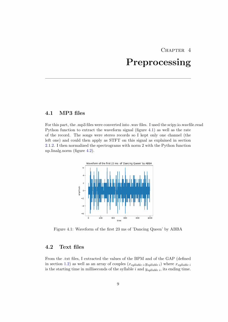
For this part, the .mp3 files were converted into .wav files. I used the scipy.io.wavfile.readPython function to extract the waveform signal (figure 4.1) as well as the rateof the record. The songs were stereo records so I kept only one channel (theleft one) and could then apply as STFT on this signal as explained in section2.1.2. I then normalized the spectrograms with norm 2 with the Python functionnp.linalg.norm (figure 4.2).

Figure 4.1: Waveform of the first 23 ms of ’Dancing Queen’ by ABBA

4.2 Text files

From the .txt files, I extracted the values of the BPM and of the GAP (definedin section 1.2) as well as an array of couples (xsyllable i,ysyllable i) where xsyllable i

is the starting time in milliseconds of the syllable i and ysyllable i, its ending time.

9

4. Preprocessing 10

(a) (b)

Figure 4.2: Spectrogram (a) and Normalized Spectrogram (b) of ’Dancing Queen’by ABBA

That array thus contains the starting and ending times of all the syllables in thesong.

xsyllable i = GAP +60000

BPM× starting time of syllable i in quarter of beats

4

ysyllable i = xsyllable i +60000

BPM× ending time of syllable i in quarter of beats

4

Note: It can be seen that the created array can be assimilated to an IBM asdescribed in section 2.2.

IBM(t, f) =

{1 if the artist is singing0 otherwise

It is clear that this representation (example on figure 4.3) is redundant andonly one row is enough to describe it. This mask can then be applied on thesong spectrogram in order to remove from it all the parts of the song when onlythe instruments are playing.

An important observation to make is that the annotation of the starting andending times in the dataset .txt files have been made during the master thesis[1] for a karaoke application and not a voice detection application. In fact, theiraccuracy is perfectly valid for lyrics display in a karaoke. However, they maynot be accurate enough for a voice detection application. Indeed, some parts ofthe singing voice are deleted and some purely instrumental parts remain. Thelabels do not match exactly with the moments when the artist is singing, whichcan make it difficult for a neural network to detect these moments.

4. Preprocessing 11

Figure 4.3: ’Ideal Binary Mask’ for Voice Detection for the song ’Sound of Silence’by Simon and Garfunkel

4.3 Smoothing

The realism of this representation can be improve by a smoother separation be-tween the times when the artist is singing and when he or she is not singing.Indeed, the voice does not often stop suddenly but its volume decreases gradu-ally. What is more, it usually does not make sense to detect a separation betweensyllables of the same words or even words of the same sentence. We can con-sider that blanks with duration of less than 50 milliseconds usually correspondto breathing and should not be detected as instrumental parts. Similarly, anisolated vocal part lasting less than a second does not in fact correspond to aword. Therefore, it seems meaningless to have ”blocks” of zeros or ones witha size smaller than 30 samples (which correspond to approximately 1 second).The binary arrays created can be smoothed by an eroding and dilatation method(figure 4.4).

The original label (the binary array which indicates whether the artist issinging) is first dilated by 7 samples so that groups of zeros or ones with lessthan 15 samples are merged. Then, an erosion of 7 samples is applied to removethe ones or the zeros that have been added on edges. At this point, there areno more groups of zeros of size less than 30 samples in-between ones. This partallows to group the syllables of same words or phrases.

A second erosion of 15 samples is applied to eliminate groups of ones of sizesmaller than 30 samples. A second dilation is done to add the ones at the edgesof groups of ones that have been deleted during the second erosion. This parthelps eliminate very short and isolated vocal parts)

4. Preprocessing 12

(a)

(b) (c)

(d) (e)

(f)

Figure 4.4: Initial label (a), label after first dilation (b), label after first erosion(c), label after second erosion (d), label after second dilation (e)

Chapter 5

Results

5.1 Speech to Text recognition

As explained in section 3.2, I used a Speech-to-Text API to retrieve the content ofthe lyrics. Surprisingly, the IBMrSpeech to Text API [6] gives very poor resultsconcerning the speech recognition on songs. I analysed the first 233 songs ofthe dataset with this tool and the mean number of words detected per song was12.7 words, the median number words detected was 5. There are obviously notenough words to allow the use the IBMrSpeech to Text API’s song transcriptionfor a Karaoke application.

Usually the best recognized songs have a very clear and close to speech singingpart and a very quiet instrumental background. However even though somewords or sentences are well detected, the resulting lyrics are not accurate enoughto use them in Karaoke. An example of one of the better recognized songs isgiven in annexe (for the song ”Don’t Worry Be Happy” by Bobby McFerrin).

These tests using the IBMrSpeech to Text API show that lyrics recognitionin songs is a more difficult problem than speech recognition in spoken language.It would take more time to adapt the methods ( for example neural networks)used in speech recognition to the lyrics recognition problem. Besides, collectingthe lyrics of songs is not the most difficult task in annotating the songs for akaraoke application. Indeed, some databases like the Music Lyrics Database [4]contain lyrics of hundreds of thousands of songs and can easily be downloaded.Therefore, I chose to focus on the collection of timing information rather on therecognition of the lyrics’ content.

5.2 Neural Network Training

5.2.1 Motivation

The goal of this semester project is to investigate how to use deep learning toannotate songs. The use of spectrograms allows to represent the song as an

13

5. Results 14

image. As Convolutional Neural Networks (CNN) are particularly effective forimage recognition [5] , the choice of this kind of network seemed natural.

5.2.2 Inputs

The song spectrograms are divided in spectrograms of size 200*1025. To makesure that the class 0 (no voice) is not over represented, the spectrograms contain-ing only zeros (which often occurs at the beginning or at the end of the song) arenot used. The size 200 corresponds to approximately 7s. 23835 inputs remain.

5.2.3 Labels

The binary arrays created as explained in section 4.2 are the labels. They are alsodivided in array of size 200 corresponding to the remaining spectrograms. Theneural network has to predict a binary array corresponding to a spectrogram,i.e. predict for every time if there is a voice in the record or not. The problemof voice detection is a binary classification problem for each time step.

5.2.4 Training

The training set is composed of 19668 examples and the test set contains 4167examples. I made sure that two examples build from the same song cannot beone in the training and the other in the test. Otherwise very similar patternscould be both in the training and test sets and create biased results.

5.2.5 Loss and Optimizer

We define the binary crossentropy loss as :

L(w) = − 1

N

N∑n=1

[yn log yn + (1− yn) log(1− yn)

], (5.1)

where w is the vector of weights and N the number of samples. yn is the groundtruth for the sample n (the label) and yn the CNN’s prediction for the samplen.

The binary crossentropy is often used in machine learning for classificationproblems involving two possible classes. When the prediction y is very close to(resp. far from) the label y, the term y log y+ (1− y) log(1− y) is very close to 0(resp. very close to 1). In order to minimize the loss L(w), the predictions haveto get closer to the labels.

The optimizer I used is AdaGrad (adaptive gradient algorithm). This is astochastic gradient descent with an adaptive learning rate which is often used

5. Results 15

in image recognition. Changes in the learning rate (in a range of 0.0001 to 0.1)made no real differences on the results.

5.2.6 Size of the convolutional filters

The filters shape makes the training focus on particular features. As explainedin [6], applying filters of size m× n with m and n bigger than 1 allows to learntime and frequency features at the same time. Filters with m = 1 helps to learntemporal features such as rythmic or tempo whereas filters with n = 1 are betterto learn frequency features such as timbre. For the purpose of voice detection,as the main difference between singing voice and instruments are the frequencydistributions and ranges. Therefore, it seems appropriate to choose a filter withlarge n. On the first layer, I chose to set the size of the filters such that n isequal to 1025 (the height of the spectrograms) and m takes much smaller values(between 3 and 19 samples).

5.2.7 Number of training samples

The first tests were made on smaller set of examples (with only 200 songs). Theresults got better when the training was done on the entire dataset.

5.2.8 Evaluation of the results

During the training the binary crossentropy losses on the training set and onthe test set were saved after each epoch in order to plot the training and testloss curves. This curves help to choose after how many epochs the model issupposed to perform the best in the classification on the test set. As long as thetest loss keeps decreasing, it makes sense to keep training the model. If the testloss increases on average for a certain number of epochs, the training has to bestopped.

The predicted array has elements which take real values between zeros andones. To evaluate a prediction, its elements are rounded to 0 or 1 (if an elementis smaller than 0.5 then it is set to 0, otherwise, it is set to 1).

The accuracy is defined as Accuracy = tp+tntp+tn+fp+fn .

• tp is the number of true positives, i.e. the number of elements in thepredicted array that are equal to one with corresponding element in labelarray also equal to one.

• tn is the number of true negatives, i.e. the number of elements in thepredicted array that are equal to zero with corresponding element in labelarray also equal to zero.

5. Results 16

• fp is the number of false positives, i.e. the number of elements in thepredicted array that are equal to one whereas corresponding element inlabel array is equal to zero.

• fn is the number of false negatives, i.e. the number of elements in thepredicted array that are equal to zero whereas corresponding element inlabel array is equal to one.

5.2.9 Results

MLP

The first tests are carried with MLPs (Multi Layer Perceptron) with only fullyconnected layers. With one hidden layer, I obtained a clearly overfitting modelwith an accuracy of 99% on the training set and a maximum of 52% on the testset. When using dropout, I could reach an accuracy of 56% on the test set.

CNN

With the a convolutional architecture, the parameters that were tuned in thedifferent simulations were:

• the number of layers from 3 to 6 layers

• the different sizes of the filters (1,7),(1,5), (1,3)

• different numbers of filters on each layer

The best accuraccy that could be obtained was of 60% in test (with 80% intraining ) with a 4 layers network with filter sizes (1025, 11) on the first layerand (1,5) on the next layers and 10 filters on each layer.

Adding a dropout layer did not change the results.

Smoothed Labels

These tests were all carried before smoothing the labels. Smoothing the la-bel brought the biggest difference I could observe in all the different trainings.As shown in figure 5.2, the test loss decreases much more when the labels aresmoothed. The confusion matrices 5.1 and 5.3 are drawn at the end of thetraining and the confusion matrices 5.2 and 5.4 after the epochs at which thetest loss reaches its lowest point. Smoothing the labels helps the test accuracyto increase from 60% to 65%.

This shows that imroving the labels is a condition to have better results.

5. Results 17

Table 5.1: Confusion matrix in training without smoothed labels

`````````````PredictionGroundtruth

0 1

0 38% 17%

1 14% 31%

Accuracy 69%

The CNN is represented in the figure 5.1.

Figure 5.1: CNN

(a) (b)

Figure 5.2: Training and Test Losses with Non Smoothed (a) and Smoothed (b)Labels

An illustration of satisfying and not satisfying predictions is given in .

5. Results 18

Table 5.2: Confusion matrix in test without smoothed labels

`````````````PredictionGroundtruth

0 1

0 35% 22%

1 18% 25%

Accuracy 60%

Table 5.3: Confusion matrix in training with smoothed labels

`````````````PredictionGroundtruth

0 1

0 22% 10%

1 19% 49%

Accuracy 71%

Table 5.4: Confusion matrix in test with smoothed labels

`````````````PredictionGroundtruth

0 1

0 18% 11%

1 23% 48%

Accuracy 66%

Chapter 6

Conclusion

The goal of this project was to annotate songs using deep learning for a karaokeapplication. The songs representation as spectrograms, their preprocessing aswell as the preprocessing of the labels are important steps.

In order to detect the singing times, different types of neural networks wereused. The results obtained with CNNs improve on the ones with MLPs. Smooth-ing the labels also refined the results.

However, the detected time information is not sufficiently accurate to prop-erly synchronize the lyrics with the song record.

Other types of neural networks could be used such as LSTM (Long short-term memory) networks, which are recurrent networks that are used in manyspeech recognition problems.

The preprocessing of the songs can be improved by using the Constant-Qtransform instead of Fourier transform (this kind of transform is preferred insome music applications) and by using the Mel-frequency cepstral coefficients(MFCCs).

One of the problems identified in this project was the lack of accuracy forvoice detection of the timing information given in the dataset described in section1.2 . The division of the lyrics in syllables is maybe not the most appropriate forvoice detection. It would maybe make more sense to use a division of the lyricsin entire words or sentences.

In order to use the first approach described in section 3.1, another datasetincluding records of songs as well as separate records of the instruments and ofthe voice could be used (for example the MedleyDb [7]).

19

Bibliography

[1] Hunziker, V.: Karaoke song generator (2016)

[2] : UltraStar. http://www.ultraguide.net [Online; accessed 05-January-2018].

[3] Simpson, A.J.R., Roma, G., Plumbley, M.D.: Deep karaoke: Extractingvocals from musical mixtures using a convolutional deep neural network.CoRR abs/1504.04658 (2015)

[4] : MLDb, The Music Lyrics Database. http://www.mldb.org/ [Online;accessed 05-January-2018].

[5] Goodfellow, I., Bengio, Y., Courville, A.: Deep Learning. MIT Press (2016)http://www.deeplearningbook.org.

[6] : CNN filter shapes discussion for music spectrograms. http:

//www.jordipons.me/cnn-filter-shapes-discussion/ [Online; accessed05-January-2018].

[7] Bittner, R.M., Salamon, J., Tierney, M., Mauch, M., Cannam, C., Bello,J.P.: Medleydb: A multitrack dataset for annotation-intensive mir research.In: ISMIR. Volume 14. (2014) 155–160

20

Appendix A

Appendix Chapter

A.1 Example of an IBMrSpeech to Text API’s test

The following lyrics give the example of the song ”Don’t Worry Be Happy” byBobby McFerrin.

In bold type are the lyrics that have been recognized.

Lyrics from [4]

Here’s a little song I wroteYou might want to sing it note for note,Don’t worry, be happyIn every life we have some trouble,When you worry you make it doubleDon’t worry, be happy

Ooh, ooh ooh ooh oo-ooh ooh oo-ooh ooh ooh oo-ooh(Don’t worry)Ooh oo-ooh ooh ooh oo-ooh(Be happy)Ooh oo-ooh oo-ooh(Don’t worry, be happy)Ooh, ooh ooh ooh oo-ooh ooh oo-ooh ooh ooh oo-ooh(Don’t worry)Ooh oo-ooh ooh ooh oo-ooh(Be happy)Ooh oo-ooh oo-ooh(Don’t worry, be happy)

Ain’t got no place to lay your head,Somebody came and took your bed,Don’t worry, be happy

A-1

Appendix Chapter A-2

The land lord say your rent is late,He may have to litigateDon’t worry, be happy(Look at me I’m happy)

Ooh, ooh ooh ooh oo-ooh ooh oo-ooh ooh ooh oo-ooh(Don’t worry)Ooh oo-ooh ooh ooh oo-ooh(Be Happy)Ooh oo-ooh oo-oohHere I give you my phone numberWhen you worry call me, I make you happyOoh, ooh ooh ooh oo-ooh ooh oo-ooh ooh ooh oo-ooh(Don’t worry)Ooh oo-ooh ooh ooh oo-ooh(Be happy)Ooh oo-ooh oo-ooh

Ooh, ooh ooh ooh oo-ooh ooh oo-ooh ooh ooh oo-ooh(Don’t worry)Ooh oo-ooh ooh ooh oo-ooh(Be Happy)Ooh oo-ooh oo-oohHere I give you my phone number,When you worry call me, I make you happyOoh, ooh ooh ooh oo-ooh ooh oo-ooh ooh ooh oo-ooh(Don’t worry)Ooh oo-ooh ooh ooh oo-ooh(Be happy)Ooh oo-ooh oo-ooh

Ain’t got no cash, ain’t got no styleAin’t got no gal to make you smileBut don’t worry, be happy’Cause when you worry your facewill frownAnd that will bring everybody down,So don’t worry, be happyDon’t worry, be happy now

Ooh, ooh ooh ooh oo-ooh ooh oo-ooh ooh ooh oo-ooh(Don’t worry)Ooh oo-ooh ooh ooh oo-ooh(Be happy)Ooh oo-ooh oo-ooh

Appendix Chapter A-3

Don’t worry, be happyOoh, ooh ooh ooh oo-ooh ooh oo-ooh ooh ooh oo-ooh(Don’t worry)Ooh oo-ooh ooh ooh oo-ooh(Be happy)Ooh oo-ooh oo-oohDon’t worry, be happy

Now there, is this song I wrote,I hope you learned it note for noteLike good little children,Don’t worry, be happyListen to what I sayIn your life expect some troubleWhen you worry you make it doubleDon’t worry, be happy, be happy now

Ooh, ooh ooh ooh oo-ooh ooh oo-ooh ooh ooh oo-ooh(Don’t worry)Ooh oo-ooh ooh ooh oo-ooh(Be happy)Ooh oo-ooh oo-oohDon’t worry, be happyOoh, ooh ooh ooh oo-ooh ooh oo-ooh ooh ooh oo-ooh(Don’t worry)Ooh oo-ooh ooh ooh oo-ooh(Be happy)Ooh oo-ooh oo-oohDon’t worry, be happy

Ooh, ooh ooh ooh oo-ooh ooh oo-ooh ooh ooh oo-ooh(Don’t worry)Ooh oo-ooh ooh ooh oo-ooh(Don’t worry, don’t worry, don’t do it, be happy)Ooh oo-ooh oo-ooh(Put a smile on your face, don’t bring everybody down)Ooh, ooh ooh ooh oo-ooh ooh oo-ooh ooh ooh oo-ooh(Don’t worry)Ooh oo-ooh ooh ooh oo-ooh(It will soon pass, whatever it is)Ooh oo-ooh oo-oohDon’t worry, be happyOoh oo-ooh oo-oohI’m not worried, I’m happy

Appendix Chapter A-4

Result from the Speech to Text API

here’s a little song Iyou might want to sing it note for note gonewe havedo you have a life and we have some trouble when you worry you may getdial tonemay have been all the way we havewhereit happenedwhere havewe haddon’tand god will blessthey are aheadsomebody came in your bed gongwe hadthey ran late and he may haveletdonand then we have ayou haveI give you my phone number when you worry aboutwhereand Capital cascade god knows thatand god will gatherandbecause whenfaced with fromthat will bring everybody downso it’s allwe have a dog where they have been thatso wherehappyand thewhereDorgan wellthis song I wroteI hope you learned itchildren don’t worrythe a happeningthey let it all out

Appendix Chapter A-5

in your life back frombut when you add atop ofdawnI havego all the waythe happydon’t worry bewearingelaborate may have awe havedon’t bring everybodygoing to wearthe sun passed with thethey have

A.2 Example of 2 predictions and labels in the testset

(a) (b)

Figure A.1: Example of a satisfying (a) and not satisfying (b) predictions