using mpifhegedus/00 - numerics/b2015 using... · using mpi : portable parallel programming with...
TRANSCRIPT


Using MPI

Scientific and Engineering ComputationWilliam Gropp and Ewing Lusk, editors; Janusz Kowalik, founding editor
A complete list of books published in the Scientific and Engineering Computationseries appears at the back of this book.
Using MPIPortable Parallel Programming with theMessage-Passing Interface
Third Edition
William GroppEwing LuskAnthony Skjellum
The MIT PressCambridge, MassachusettsLondon, England
c© 2014 Massachusetts Institute of Technology
All rights reserved. No part of this book may be reproduced in any form by any electronic ormechanical means (including photocopying, recording, or information storage and retrieval)without permission in writing from the publisher.
This book was set in LATEX by the authors and was printed and bound in the United States ofAmerica.
Library of Congress Cataloging-in-Publication Data
Gropp, William.Using MPI : portable parallel programming with the Message-Passing Interface / WilliamGropp, Ewing Lusk, and Anthony Skjellum. — Third edition.
p. cm. — (Scientific and engineering computation)Includes bibliographical references and index.ISBN 978-0-262-52739-2 (pbk. : alk. paper)1. Parallel programming (Computer science) 2. Parallel computers—Programming. 3. Computerinterfaces. I. Lusk, Ewing. II. Skjellum, Anthony. III. Title. IV. Title: Using Message-PassingInterface.QA76.642.G76 2014005.2’75—dc23
2014033587
10 9 8 7 6 5 4 3 2 1

To Patty, Brigid, and Jennifer
Contents
Series Foreword xiii
Preface to the Third Edition xv
Preface to the Second Edition xix
Preface to the First Edition xxi
1 Background 1
1.1 Why Parallel Computing? 1
1.2 Obstacles to Progress 2
1.3 Why Message Passing? 3
1.3.1 Parallel Computational Models 3
1.3.2 Advantages of the Message-Passing Model 9
1.4 Evolution of Message-Passing Systems 10
1.5 The MPI Forum 11
2 Introduction to MPI 13
2.1 Goal 13
2.2 What Is MPI? 13
2.3 Basic MPI Concepts 14
2.4 Other Interesting Features of MPI 18
2.5 Is MPI Large or Small? 20
2.6 Decisions Left to the Implementor 21
3 Using MPI in Simple Programs 23
3.1 A First MPI Program 23
3.2 Running Your First MPI Program 28
3.3 A First MPI Program in C 29
3.4 Using MPI from Other Languages 29
3.5 Timing MPI Programs 31
3.6 A Self-Scheduling Example: Matrix-Vector Multiplication 32
3.7 Studying Parallel Performance 38
3.7.1 Elementary Scalability Calculations 39

viii Contents
3.7.2 Gathering Data on Program Execution 41
3.7.3 Instrumenting a Parallel Program with MPELogging
42
3.7.4 Events and States 43
3.7.5 Instrumenting the Matrix-Matrix Multiply Program 43
3.7.6 Notes on Implementation of Logging 47
3.7.7 Graphical Display of Logfiles 48
3.8 Using Communicators 49
3.9 Another Way of Forming New Communicators 55
3.10 A Handy Graphics Library for Parallel Programs 57
3.11 Common Errors and Misunderstandings 60
3.12 Summary of a Simple Subset of MPI 62
3.13 Application: Computational Fluid Dynamics 62
3.13.1 Parallel Formulation 63
3.13.2 Parallel Implementation 65
4 Intermediate MPI 69
4.1 The Poisson Problem 70
4.2 Topologies 73
4.3 A Code for the Poisson Problem 81
4.4 Using Nonblocking Communications 91
4.5 Synchronous Sends and “Safe” Programs 94
4.6 More on Scalability 95
4.7 Jacobi with a 2-D Decomposition 98
4.8 An MPI Derived Datatype 100
4.9 Overlapping Communication and Computation 101
4.10 More on Timing Programs 105
4.11 Three Dimensions 106
4.12 Common Errors and Misunderstandings 107
4.13 Application: Nek5000/NekCEM 108
5 Fun with Datatypes 113
Contents ix
5.1 MPI Datatypes 113
5.1.1 Basic Datatypes and Concepts 113
5.1.2 Derived Datatypes 116
5.1.3 Understanding Extents 118
5.2 The N-Body Problem 119
5.2.1 Gather 120
5.2.2 Nonblocking Pipeline 124
5.2.3 Moving Particles between Processes 127
5.2.4 Sending Dynamically Allocated Data 132
5.2.5 User-Controlled Data Packing 134
5.3 Visualizing the Mandelbrot Set 136
5.3.1 Sending Arrays of Structures 144
5.4 Gaps in Datatypes 146
5.5 More on Datatypes for Structures 148
5.6 Deprecated and Removed Functions 149
5.7 Common Errors and Misunderstandings 150
5.8 Application: Cosmological Large-Scale Structure Formation 152
6 Parallel Libraries 155
6.1 Motivation 155
6.1.1 The Need for Parallel Libraries 155
6.1.2 Common Deficiencies of Early Message-PassingSystems
156
6.1.3 Review of MPI Features That Support Libraries 158
6.2 A First MPI Library 161
6.3 Linear Algebra on Grids 170
6.3.1 Mappings and Logical Grids 170
6.3.2 Vectors and Matrices 175
6.3.3 Components of a Parallel Library 177
6.4 The LINPACK Benchmark in MPI 179
6.5 Strategies for Library Building 183
6.6 Examples of Libraries 184
6.7 Application: Nuclear Green’s Function Monte Carlo 185
x Contents
7 Other Features of MPI 189
7.1 Working with Global Data 189
7.1.1 Shared Memory, Global Data, and DistributedMemory
189
7.1.2 A Counter Example 190
7.1.3 The Shared Counter Using Polling Instead of anExtra Process
193
7.1.4 Fairness in Message Passing 196
7.1.5 Exploiting Request-Response Message Patterns 198
7.2 Advanced Collective Operations 201
7.2.1 Data Movement 201
7.2.2 Collective Computation 201
7.2.3 Common Errors and Misunderstandings 206
7.3 Intercommunicators 208
7.4 Heterogeneous Computing 216
7.5 Hybrid Programming with MPI and OpenMP 217
7.6 The MPI Profiling Interface 218
7.6.1 Finding Buffering Problems 221
7.6.2 Finding Load Imbalances 223
7.6.3 Mechanics of Using the Profiling Interface 223
7.7 Error Handling 226
7.7.1 Error Handlers 226
7.7.2 Example of Error Handling 229
7.7.3 User-Defined Error Handlers 229
7.7.4 Terminating MPI Programs 232
7.7.5 Common Errors and Misunderstandings 232
7.8 The MPI Environment 234
7.8.1 Processor Name 236
7.8.2 Is MPI Initialized? 236
7.9 Determining the Version of MPI 237
7.10 Other Functions in MPI 239
7.11 Application: No-Core Configuration InteractionCalculations in Nuclear Physics
240

Contents xi
8 Understanding How MPI ImplementationsWork
245
8.1 Introduction 245
8.1.1 Sending Data 245
8.1.2 Receiving Data 246
8.1.3 Rendezvous Protocol 246
8.1.4 Matching Protocols to MPI’s Send Modes 247
8.1.5 Performance Implications 248
8.1.6 Alternative MPI Implementation Strategies 249
8.1.7 Tuning MPI Implementations 249
8.2 How Difficult Is MPI to Implement? 249
8.3 Device Capabilities and the MPI Library Definition 250
8.4 Reliability of Data Transfer 251
9 Comparing MPI with Sockets 253
9.1 Process Startup and Shutdown 255
9.2 Handling Faults 257
10 Wait! There’s More! 259
10.1 Beyond MPI-1 259
10.2 Using Advanced MPI 260
10.3 Will There Be an MPI-4? 261
10.4 Beyond Message Passing Altogether 261
10.5 Final Words 262
Glossary of Selected Terms 263
A The MPE Multiprocessing Environment 273
A.1 MPE Logging 273
A.2 MPE Graphics 275
A.3 MPE Helpers 276
B MPI Resources Online 279
xii Contents
C Language Details 281
C.1 Arrays in C and Fortran 281
C.1.1 Column and Row Major Ordering 281
C.1.2 Meshes vs. Matrices 281
C.1.3 Higher Dimensional Arrays 282
C.2 Aliasing 285
References 287
Subject Index 301
Function and Term Index 305
Series Foreword
The Scientific and Engineering Series from MIT Press presents accessible accounts
of computing research areas normally presented in research papers and specialized
conferences. Elements of modern computing that have appeared thus far in the
series include parallelism, language design and implementation, system software,
and numerical libraries. The scope of the series continues to expand with the
spread of ideas from computing into new aspects of science.
This book in the series is the first of two books describing how to use the Message-
Passing Interface (MPI), a communication library for both parallel computers and
workstation networks. MPI has been developed as a standard for message passing
and related operations. Its adoption by both users and implementors is providing
the parallel programming community with the portability and features needed to
develop application programs and parallel libraries that tap the power of today’s
(and tomorrow’s) high-performance computers.
William Gropp and Ewing Lusk, Editors

Preface to the Third Edition
In the fifteen years since the second edition of Using MPI was published, in 1999,
high-performance computing (HPC) has undergone many changes. Some aspects of
HPC have been disruptive and revolutionary; but others, no less significant, have
been gradual and evolutionary. This edition of Using MPI updates the second
edition to bring our presentation of the Message-Passing Interface (MPI) standard
into line with these changes.
The most dramatic change has been in parallel computing hardware. The speed
(cycle rate) of individual processing units has leveled off because of power and heat-
dissipation constraints, causing parallelism to become mainstream and, for HPC,
putting increased pressure on the scale of parallelism. Computer vendors have re-
sponded. The preface to the second edition refers to “the very largest computers
in the world, with thousands of processors.” Today, applications run on comput-
ers with millions of processors. The processors referred to at that time have also
undergone substantial change. Multiple processors sharing memory, multicore pro-
cessors, with multiple hardware threads per core, perhaps with attached graphical
processing units (GPUs), are now common in HPC machines and indeed in all
computers.
In the programming languages area, change has been less dramatic. HPC appli-
cations still rely on Fortran, C, and C++ for the compute-intensive parts of their
algorithms (except for GPUs), although these standard languages have themselves
evolved. C now means C11, and (for our purposes here) Fortran means Fortran
2008. OpenMP has emerged as the most widely used approach in computational
science to the shared-memory programming appropriate for multiprocessor nodes
and multicore processors. GPU programming can be said to be where message
passing was in the early 1990s, with competing application programming interfaces
(APIs) and a search for a standard that will provide portability among competing
hardware devices without sacrificing performance.
Applications have changed even less, although the increased scale of the largest
machines has stimulated the search for more scalable algorithms and the use of
libraries that provide new levels of scalability. Adoption of radically new pro-
gramming models and languages has been conservative: most large applications
are written in Fortran, C, or C++, with parallelism provided by MPI (or libraries
written on top of it), OpenMP, and (increasingly) vendor-specific GPU-executed
subsections. Reliance on MPI has remained central to application development
and/or execution.
MPI itself has changed in some ways but not others. Basic functions have not
changed: the first example code from the first edition of this book is still valid. The
xvi Preface to the Third Edition
basic point-to-point and collective communication functions are unaltered. The
largest changes to the MPI standard are those made by the MPI-3 Forum. After
a “rest period” of some fifteen years, the MPI Forum reconstituted itself in 2008,
with both veteran and new members, to bring the MPI standard up to date with
respect to the new developments in hardware capabilities, core language evolution,
the needs of applications, and the experience gained over the years by computer
vendors, MPI implementors, and users. The changes included substantial additions
to the API, especially in the area of remote memory operations, but also removal or
replacement of some functions and a few changes that affect even simple programs.
The most substantive changes are described in a companion volume to this one,
Using Advanced MPI, but all the changes by the MPI-3 Forum that affect the
material described here are incorporated in this volume.
About the Third Edition
This third edition of Using MPI contains many updates to the second edition.
• All example code has been brought up to date with respect to modern C and
Fortran.
• MPI-3 changes that are relevant to our discussions and examples are fully
reflected in both the example code and the text. All deprecated functions
have been removed, and where new, better ways of doing things have been
made available, they are used.
• The C++ bindings, which were removed in MPI-3, have vanished, leaving
only a brief discussion of how to use MPI in C++ programs.
• Applications have been updated or replaced with those more typical of current
practice.
• The references have been updated to reflect the substantial attention MPI
has received in academic and other literature.
Our order of presentation again is guided by the level of complexity in the al-
gorithms we study. This tutorial approach differs substantially from that given in
more formal presentations of the MPI standard such as [112]. The overall structure
of this edition is little changed from that of the previous edition; however, each
individual chapter does include substantial updates. Among other changes, the ap-
plications sections, which have been contributed by active computational scientists

Preface to the Third Edition xvii
using MPI, have as their primary audience those who are interested in how MPI
has been used in a specific scientific domain. These sections may easily be skipped
by the general reader. We include them to demonstrate that MPI has been used in
quite advanced application programs.
We begin in Chapter 1 with a brief overview of the current situation in parallel
computing environments, the message-passing model, and the process that pro-
duced MPI. This chapter has been updated to describe in more detail the changes
in HPC environments that have occurred since the previous edition, as discussed
briefly above. We have also updated the account of MPI Forum activities to describe
the recent work of the MP-3 Forum.
Chapter 2 introduces the basic concepts that arise from the message-passing
model itself and how MPI augments these basic concepts to create a full-featured,
high-performance-capable interface. Parts of this chapter have been completely
rewritten.
In Chapter 3 we set the pattern for the remaining chapters. We present several
examples and the small number of MPI functions that are required to express them.
We describe how to execute the examples using one widely used MPI implementa-
tion and how to investigate the performance of these programs using a graphical
performance-analysis tool. The previous edition’s application in this chapter has
been moved to the libraries chapter, written using only the MPI functions intro-
duced in this chapter, together with a new library described there.
Chapter 4 rounds out the basic features of MPI by focusing on a particular appli-
cation prototypical of a large family: solution of the Poisson problem. We introduce
MPI’s facilities for application-oriented process structures called virtual topologies.
Using performance analysis tools, we illustrate how to improve performance using
slightly more advanced MPI message-passing functions. The discussion of non-
blocking operations here has been expanded. We conclude with a discussion of a
production code currently being used to investigate a number of problems in fluid
mechanics.
Some of the more advanced features for message passing provided by MPI are
covered in Chapter 5. We use the N-body problem as a setting for much of the
discussion. We complete our discussion of derived datatypes with a focus on features
that have been added in MPI-3. Our application is a cosmology simulation that
uses advanced approaches to N-body problems.
We believe that the majority of programmers of parallel computers will, in the
long run, access parallelism through libraries. Indeed, enabling the construction of
robust libraries is one of the primary motives behind the MPI effort, and perhaps
its single most distinguishing feature when compared with other parallel program-

xviii Preface to the Third Edition
ming environments. In Chapter 6 we address this issue with a series of examples.
We introduce a new library (the Asynchronous Dynamic Load Balancing (ADLB)
library) and describe its use in simplifying a nuclear structure application while
increasing its scalability.
MPI contains a variety of advanced features that will only have been touched on
or presented in their simplest form at this point in the book. These features include
elaborate collective data-distribution and data-collection schemes, error handling,
and facilities for implementing client-server applications. In Chapter 7 we fill out
the description of these features using further examples taken from applications.
Our application in this chapter is a sophisticated hybrid calculation for nuclear
theory.
In Chapter 8 we discuss what one finds “under the hood” in implementations of
MPI. Understanding the choices available to MPI implementors can provide insight
into the behavior of MPI programs in various computing environments. Changes in
communication hardware and ubiquity of multithreading motivate updates to the
previous edition’s treatment.
Chapter 9 presents a comparison of MPI with sockets, a standard interface for
sending messages between processes on different machines for both Unix and Mi-
crosoft systems. Examining the similarities and differences helps one understand
the assumptions that MPI makes about underlying system services.
Chapter 10 contains a brief summary of the material in the companion volume
to this book, which includes topics from both MPI-2 and MPI-3. We conclude with
a few thoughts on the future of MPI.
We include a glossary of terms used in this book. The appendices include material
that would have been out of place in the main text. Appendix A describes the MPE
library that we use in several of our examples and gives its Fortran and C bindings.
Appendix B provides pointers to supplementary material for this book, including
complete source code for the examples, and related MPI materials that are available
on the net. Appendix C discusses some issues of C and Fortran that are relevant
to MPI and may be unfamiliar to some readers. It has been updated to reflect new
developments in Fortran and particular issues related to MPI-3.
Acknowledgments for the Third Edition
We gratefully acknowledge the careful and thoughtful work of our copy editor, Gail
Pieper. We are also grateful to those who contributed application examples: Steve
Pieper, James Vary and Pieter Maris, Salman Habib and Hal Finkel, and Paul
Fischer.
Preface to the Second Edition
When Using MPI was first published in 1994, the future of MPI was unknown.
The MPI Forum had just concluded its work on the Standard, and it was not yet
clear whether vendors would provide optimized implementations or whether users
would select MPI for writing new parallel programs or would port existing codes
to MPI.
Now the suspense is over. MPI is available everywhere and widely used, in en-
vironments ranging from small workstation networks to the very largest computers
in the world, with thousands of processors. Every parallel computer vendor offers
an MPI implementation, and multiple implementations are freely available as well,
running on a wide variety of architectures. Applications large and small have been
ported to MPI or written as MPI programs from the beginning, and MPI is taught
in parallel programming courses worldwide.
In 1995, the MPI Forum began meeting again. It revised in a compatible way
and significantly extended the MPI specification, releasing version 1.2 (covering the
topics included in the original, 1.0 specification) and version 2.0 (covering entirely
new topics) in the summer of 1997. In this book, we update the original Using
MPI to reflect these later decisions of the MPI Forum. Roughly speaking, this
book covers the use of MPI 1.2, while Using MPI 2 (published by MIT Press as a
companion volume to this book) covers extensions in MPI 2.0. New topics in MPI-
2 include parallel I/O, one-sided operations, and dynamic process management.
However, many topics relevant to the original MPI functions were modified as well,
and these are discussed here. Thus this book can be viewed as the up-to-date
version of the topics covered in the original edition.
About the Second Edition
This second edition of Using MPI: Portable Programming with the Message-Passing
Interface contains many changes from and additions to the first edition.
• We have added many new examples and have added additional explanations
to the examples from the first edition.
• A section on common errors and misunderstandings has been added to several
chapters.
• We have added new material on the performance impact of choices among
alternative MPI usages.
xx Preface to the Second Edition
• A chapter on implementation issues has been added to increase understanding
of how and why various MPI implementations may differ, particularly with
regard to performance.
• Since “Fortran” now means Fortran 90 (or Fortran 95 [17]), all Fortran ex-
amples have been updated to Fortran 90 syntax. We do, however, explain the
small modifications necessary to run the examples in Fortran 77.
• We have added the new functions from the MPI 1.2 specification, and also
those from MPI 2.0 whose exposition seems to belong with functions from
MPI 1.2.
• We describe new tools in the MPE toolkit, reflecting their evolution since the
publication of the first edition.
• The chapter on converting to MPI from earlier message-passing systems has
been greatly revised, now that many of those systems have been completely
supplanted by MPI. We include a comparison of MPI syntax and semantics
with PVM, since conversion of programs from PVM to MPI is still going on.
We also compare MPI with the use of Unix sockets.
• Some functions in MPI 1.0 are now deprecated, since better definitions have
now been made. These are identified and their replacements described.
• Errors, particularly those in the example programs, have been corrected.
[To preclude possible confusion on the part of the reader, the outline of the second
edition that occurred here has been omitted.]
Acknowledgments for the Second Edition
We thank Peter Lyster of NASA’s Goddard Space Flight Center for sharing his
marked-up copy of the first edition of Using MPI with us. We thank Puri Banga-
lore, Nicholas Carriero, Robert van de Geijn, Peter Junglas, David Levine, Bryan
Putnam, Bill Saphir, David J. Schneider, Barry Smith, and Stacey Smith for send-
ing in errata for the first edition (and anyone that we’ve forgotten), and Anand Pillai
for correcting some of the examples in Chapter 6. The reviewers of the prospectus
for this book offered many helpful suggestions for topics. We thank Gail Pieper for
her careful and knowledgeable editing.
Preface to the First Edition
About This Book
During 1993, a broadly based group of parallel computer vendors, software writers,
and application scientists collaborated on the development of a standard portable
message-passing library definition called MPI, for Message-Passing Interface. MPI
is a specification for a library of routines to be called from C and Fortran programs.
As of mid-1994, a number of implementations are in progress, and applications are
already being ported.
Using MPI: Portable Parallel Programming with the Message-Passing Interface
is designed to accelerate the development of parallel application programs and li-
braries by demonstrating how to use the new standard. It fills the gap among
introductory texts on parallel computing, advanced texts on parallel algorithms for
scientific computing, and user manuals of various parallel programming languages
and systems. Each topic begins with simple examples and concludes with real appli-
cations running on today’s most powerful parallel computers. We use both Fortran
(Fortran 77) and C. We discuss timing and performance evaluation from the outset,
using a library of useful tools developed specifically for this presentation. Thus this
book is not only a tutorial on the use of MPI as a language for expressing parallel
algorithms, but also a handbook for those seeking to understand and improve the
performance of large-scale applications and libraries.
Without a standard such as MPI, getting specific about parallel programming has
necessarily limited one’s audience to users of some specific system that might not
be available or appropriate for other users’ computing environments. MPI provides
the portability necessary for a concrete discussion of parallel programming to have
wide applicability. At the same time, MPI is a powerful and complete specification,
and using this power means that the expression of many parallel algorithms can
now be done more easily and more naturally than ever before, without giving up
efficiency.
Of course, parallel programming takes place in an environment that extends be-
yond MPI. We therefore introduce here a small suite of tools that computational
scientists will find useful in measuring, understanding, and improving the perfor-
mance of their parallel programs. These tools include timing routines, a library to
produce an event log for post-mortem program visualization, and a simple real-time
graphics library for run-time visualization. Also included are a number of utilities
that enhance the usefulness of the MPI routines themselves. We call the union of
these libraries MPE, for MultiProcessing Environment. All the example programs

xxii Preface to the First Edition
and tools are freely available, as is a model portable implementation of MPI itself
developed by researchers at Argonne National Laboratory and Mississippi State
University [59].
Our order of presentation is guided by the level of complexity in the parallel
algorithms we study; thus it differs substantially from the order in more formal
presentations of the standard.
[To preclude possible confusion on the part of the reader, the outline of the first
edition that occurred here has been omitted.]
In addition to the normal subject index, there is an index for the definitions and
usage examples for the MPI functions used in this book. A glossary of terms used
in this book may be found before the appendices.
We try to be impartial in the use of Fortran and C for the book’s examples;
many examples are given in each language. The MPI standard has tried to keep
the syntax of its calls similar in Fortran and C; for the most part they differ only
in case (all capitals in Fortran, although most compilers will accept all lower case
as well, while in C only the “MPI” and the next letter are capitalized), and in the
handling of the return code (the last argument in Fortran and the returned value
in C). When we need to refer to an MPI function name without specifying whether
it is Fortran or C, we will use the C version, just because it is a little easier to read
in running text.
This book is not a reference manual, in which MPI routines would be grouped
according to functionality and completely defined. Instead we present MPI routines
informally, in the context of example programs. Precise definitions are given in [93].
Nonetheless, to increase the usefulness of this book to someone working with MPI,
we have provided for each MPI routine that we discuss a reminder of its calling
sequence, in both Fortran and C. These listings can be found set off in boxes
scattered throughout the book, located near the introduction of the routines they
contain. In the boxes for C, we use ANSI C style declarations. Arguments that can
be of several types (typically message buffers) are typed as void*. In the Fortran
boxes the types of such arguments are marked as being of type <type>. This
means that one of the appropriate Fortran data types should be used. To find the
“binding box” for a given MPI routine, one should use the appropriate bold-face
reference in the Function Index (f90 for Fortran, C for C).
Acknowledgments
Our primary acknowledgment is to the Message Passing Interface Forum (MPIF),
whose members devoted their best efforts over the course of a year and a half to
Preface to the First Edition xxiii
producing MPI itself. The appearance of such a standard has enabled us to collect
and coherently express our thoughts on how the process of developing application
programs and libraries for parallel computing environments might be carried out.
The aim of our book is to show how this process can now be undertaken with more
ease, understanding, and probability of success than has been possible before the
appearance of MPI.
The MPIF is producing both a final statement of the standard itself and an
annotated reference manual to flesh out the standard with the discussion necessary
for understanding the full flexibility and power of MPI. At the risk of duplicating
acknowledgments to be found in those volumes, we thank here the following MPIF
participants, with whom we collaborated on the MPI project. Special effort was
exerted by those who served in various positions of responsibility: Lyndon Clarke,
James Cownie, Jack Dongarra, Al Geist, Rolf Hempel, Steven Huss-Lederman,
Bob Knighten, Richard Littlefield, Steve Otto, Mark Sears, Marc Snir, and David
Walker. Other participants included Ed Anderson, Joe Baron, Eric Barszcz, Scott
Berryman, Rob Bjornson, Anne Elster, Jim Feeney, Vince Fernando, Sam Fineberg,
Jon Flower, Daniel Frye, Ian Glendinning, Adam Greenberg, Robert Harrison,
Leslie Hart, Tom Haupt, Don Heller, Tom Henderson, Alex Ho, C.T. Howard Ho,
John Kapenga, Bob Leary, Arthur Maccabe, Peter Madams, Alan Mainwaring,
Oliver McBryan, Phil McKinley, Charles Mosher, Dan Nessett, Peter Pacheco,
Howard Palmer, Paul Pierce, Sanjay Ranka, Peter Rigsbee, Arch Robison, Erich
Schikuta, Ambuj Singh, Alan Sussman, Robert Tomlinson, Robert G. Voigt, Dennis
Weeks, Stephen Wheat, and Steven Zenith.
While everyone listed here made positive contributions, and many made major
contributions, MPI would be far less important if it had not had the benefit of the
particular energy and articulate intelligence of James Cownie of Meiko, Paul Pierce
of Intel, and Marc Snir of IBM.
Support for the MPI meetings came in part from ARPA and NSF under grant
ASC-9310330, NSF Science and Technology Center Cooperative Agreement No.
CCR-8809615, and the Commission of the European Community through Esprit
Project P6643. The University of Tennessee kept MPIF running financially while
the organizers searched for steady funding.
The authors specifically thank their employers, Argonne National Laboratory
and Mississippi State University, for the time and resources to explore the field of
parallel computing and participate in the MPI process. The first two authors were
supported by the U.S. Department of Energy under contract W-31-109-Eng-38.
The third author was supported in part by the NSF Engineering Research Center
for Computational Field Simulation at Mississippi State University.
xxiv Preface to the First Edition
The MPI Language Specification is copyrighted by the University of Tennessee
and will appear as a special issue of International Journal of Supercomputer Appli-
cations, published by MIT Press. Both organizations have dedicated the language
definition to the public domain.
We also thank Nathan Doss of Mississippi State University and Hubertus Franke
of the IBM Corporation, who participated in the early implementation project that
has allowed us to run all of the examples in this book. We thank Ed Karrels, a
student visitor at Argonne, who did most of the work on the MPE library and the
profiling interface examples. He was also completely responsible for the new version
of the upshot program for examining logfiles.
We thank James Cownie of Meiko and Brian Grant of the University of Wash-
ington for reading the manuscript and making many clarifying suggestions. Gail
Pieper vastly improved the prose. We also thank those who have allowed us to
use their research projects as examples: Robert Harrison, Dave Levine, and Steven
Pieper.
Finally we thank several Mississippi State University graduate students whose
joint research with us (and each other) have contributed to several large-scale ex-
amples in the book. The members of the Parallel Scientific Computing class in the
Department of Computer Science at MSU, spring 1994, helped debug and improve
the model implementation and provided several projects included as examples in
this book. We specifically thank Purushotham V. Bangalore, Ramesh Pankajak-
shan, Kishore Viswanathan, and John E. West for the examples (from the class and
research) that they have provided for us to use in the text.

Using MPI
1 Background
In this chapter we survey the setting in which the MPI standard has evolved, from
the current situation in parallel computing and the status of the message-passing
model for parallel computation to the actual process by which MPI was developed.
1.1 Why Parallel Computing?
Fast computers have stimulated the rapid growth of a new way of doing science.
The two broad classical branches of theoretical science and experimental science
have been joined by computational science. Computational scientists simulate on
supercomputers phenomena too complex to be reliably predicted by theory and too
dangerous or expensive to be reproduced in the laboratory. Successes in compu-
tational science have caused demand for supercomputing resources to rise sharply
over the past twenty years.
During this time parallel computers have evolved from experimental contraptions
in laboratories to become the everyday tools of computational scientists who need
the ultimate in computer resources in order to solve their problems.
Several factors have stimulated this evolution. It is not only that the speed of
light and the effectiveness of heat dissipation impose physical limits on the speed
of a single computer. (To pull a bigger wagon, it is easier to add more oxen than
to grow a gigantic ox.) It is also that the cost of advanced single-processor com-
puters increases more rapidly than their power. (Large oxen are expensive.) And
price/performance ratios become really favorable if the required computational re-
sources can be found instead of purchased. This factor caused many sites to exploit
existing workstation networks, originally purchased to do modest computational
chores, as SCANs (SuperComputers At Night) by utilizing the workstation network
as a parallel computer. And as personal computer (PC) performance increased and
prices fell steeply, both for the PCs themselves and the network hardware neces-
sary to connect them, dedicated clusters of PC workstations provided significant
computing power on a budget. The largest of these clusters, assembled out of com-
mercial off-the-shelf (COTS) parts, competed with offerings from traditional super-
computer vendors. One particular flavor of this approach, involving open source
system software and dedicated networks, acquired the name “Beowulf” [113]. Fur-
ther, the growth in performance and capacity of wide-area networks (WANs) has
made it possible to write applications that span the globe. Many researchers are
exploring the concept of a “grid” [50] of computational resources and connections
that is in some ways analogous to the electric power grid.
2 Chapter 1
Thus, considerations of both peak performance and price/performance are push-
ing large-scale computing in the direction of parallelism. So why hasn’t parallel
computing taken over? Why isn’t every program a parallel one?
1.2 Obstacles to Progress
Barriers to the widespread use of parallelism are in all three of the usual large
subdivisions of computing: hardware, algorithms, and software.
In the hardware arena, we are still trying to build intercommunication networks
(often called switches) that keep up with speeds of advanced single processors.
Although not needed for every application (many successful parallel programs use
Ethernet for their communication environment and some even use electronic mail),
in general, faster computers require faster switches to enable most applications to
take advantage of them. Over the past ten years much progress has been made
in this area, and today’s parallel supercomputers have a better balance between
computation and communication than ever before.
Algorithmic research has contributed as much to the speed of modern parallel
programs as has hardware engineering research. Parallelism in algorithms can be
thought of as arising in three ways: from the physics (independence of physical pro-
cesses), from the mathematics (independence of sets of mathematical operations),
and from the programmer’s imagination (independence of computational tasks). A
bottleneck occurs, however, when these various forms of parallelism in algorithms
must be expressed in a real program to be run on a real parallel computer. At this
point, the problem becomes one of software.
The biggest obstacle to the spread of parallel computing and its benefits in econ-
omy and power is inadequate software. The author of a parallel algorithm for
an important computational science problem may find the current software envi-
ronment obstructing rather than smoothing the path to use of the very capable,
cost-effective hardware available.
Part of the obstruction consists of what is not there. Compilers that automat-
ically parallelize sequential algorithms remain limited in their applicability. Al-
though much research has been done and parallelizing compilers work well on some
programs, the best performance is still obtained when the programmer supplies the
parallel algorithm. If parallelism cannot be provided automatically by compilers,
what about libraries? Here some progress has occurred, but the barriers to writing
libraries that work in multiple environments have been great. The requirements of
libraries and how these requirements are addressed by MPI are the subject matter
of Chapter 6.
Background 3
Other parts of the obstruction consist of what is there. The ideal mechanism for
communicating a parallel algorithm to a parallel computer should be expressive,
efficient, and portable. Before MPI, various mechanisms all represented compro-
mises among these three goals. Some vendor-specific libraries were efficient but
not portable, and in most cases minimal with regard to expressiveness. High-level
languages emphasize portability over efficiency. And programmers are never satis-
fied with the expressivity of their programming language. (Turing completeness is
necessary, but not sufficient.)
MPI is a compromise too, of course, but its design has been guided by a vivid
awareness of these goals in the context of the next generation of parallel systems.
It is portable. It is designed to impose no semantic restrictions on efficiency; that
is, nothing in the design (as opposed to a particular implementation) forces a loss
of efficiency. Moreover, the deep involvement of vendors in MPI’s definition has en-
sured that vendor-supplied MPI implementations can be efficient. As for expressiv-
ity, MPI is designed to be a convenient, complete definition of the message-passing
model, the justification for which we discuss in the next section.
1.3 Why Message Passing?
To put our discussion of message passing in perspective, we briefly review informally
the principal parallel computational models. We focus then on the advantages of
the message-passing model.
1.3.1 Parallel Computational Models
A computational model is a conceptual view of the types of operations available
to a program. It does not include the specific syntax of a particular programming
language or library, and it is (almost) independent of the underlying hardware
that supports it. That is, any of the models we discuss can be implemented on
any modern parallel computer, given a little help from the operating system. The
effectiveness of such an implementation, however, depends on the gap between the
model and the machine.
Parallel computational models form a complicated structure. They can be differ-
entiated along multiple axes: whether memory is physically shared or distributed,
how much communication is in hardware or software, exactly what the unit of ex-
ecution is, and so forth. The picture is made confusing by the fact that software
can provide an implementation of any computational model on any hardware. This
section is thus not a taxonomy; rather, we wish to define our terms in order to
4 Chapter 1
delimit clearly our discussion of the message-passing model, which is the focus of
MPI.
Data parallelism. Although parallelism occurs in many places and at many lev-
els in a modern computer, one of the first places it was made available to the
programmer was in vector processors. Indeed, the vector machine began the cur-
rent age of supercomputing. The vector machine’s notion of operating on an array
of similar data items in parallel during a single operation was extended to include
the operation of whole programs on collections of data structures, as in SIMD
(single-instruction, multiple-data) machines such as the ICL DAP and the Think-
ing Machines CM-2. The parallelism need not necessarily proceed instruction by
instruction in lock step for it to be classified as data parallel. Data parallelism
is now more a programming style than a computer architecture, and the CM-2 is
extinct.
At whatever level, the model remains the same: the parallelism comes entirely
from the data and the program itself looks much like a sequential program. The
partitioning of data that underlies this model may be done by a compiler. High
Performance Fortran (HPF) [79] defined extensions to Fortran that allowed the
programmer to specify a partitioning and that the compiler would translate into
code, including any communication between processes. While HPF is rarely used
anymore, some of these ideas have been incorporated into languages such as Chapel
or X10.
Compiler directives such as those defined by OpenMP [97] allow the program-
mer a way to provide hints to the compiler on where to find data parallelism in
sequentially coded loops.
Data parallelism has made a dramatic comeback in the form of graphical process-
ing units, or GPUs. Originally developed as attached processors to support video
games, they are now being incorporated into general-purpose computers as well.
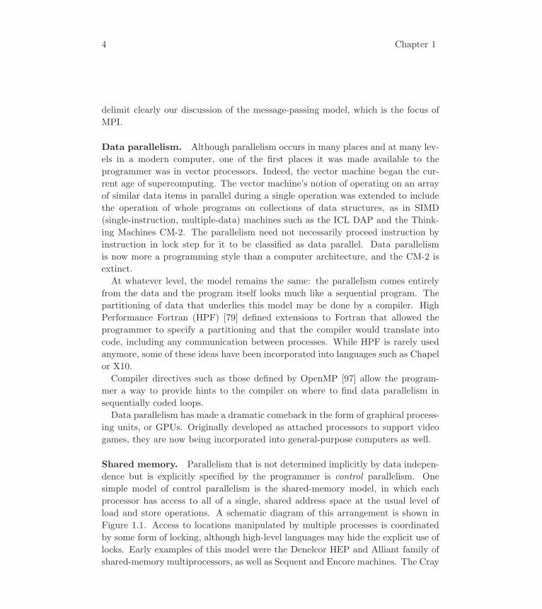
Shared memory. Parallelism that is not determined implicitly by data indepen-
dence but is explicitly specified by the programmer is control parallelism. One
simple model of control parallelism is the shared-memory model, in which each
processor has access to all of a single, shared address space at the usual level of
load and store operations. A schematic diagram of this arrangement is shown in
Figure 1.1. Access to locations manipulated by multiple processes is coordinated
by some form of locking, although high-level languages may hide the explicit use of
locks. Early examples of this model were the Denelcor HEP and Alliant family of
shared-memory multiprocessors, as well as Sequent and Encore machines. The Cray

Background 5
Processes
Address space
Figure 1.1: The shared-memory model
parallel vector machines, as well as the SGI Power Challenge series, were also of
this same model. Now there are many small-scale shared-memory machines, often
called “symmetric multiprocessors” (SMPs). Over the years, “small” has evolved
from two or four (now common on laptops) to as many as sixty-four processors
sharing one memory system.
Making “true” shared-memory machines with more than a few tens of proces-
sors is difficult (and expensive). To achieve the shared-memory model with large
numbers of processors, one must allow some memory references to take longer than
others. The most common shared-memory systems today are single-chip multicore
processors or nodes consisting of a few multicore processors. Such nodes can be
assembled into very large distributed-memory machines. A variation on the shared-
memory model occurs when processes have a local memory (accessible by only one
process) and also share a portion of memory (accessible by some or all of the other
processes). The Linda programming model [37] is of this type.
Message passing. The message-passing model posits a set of processes that have
only local memory but are able to communicate with other processes by sending
and receiving messages. It is a defining feature of the message-passing model that
data transfer from the local memory of one process to the local memory of another
requires operations to be performed by both processes. Since MPI is a specific re-
alization of the message-passing model, we discuss message passing in detail below.
In Figure 1.2 we don’t show a specific communication network because it is not
part of the computational model. The IBM Blue Gene/P had a three-dimensional
mesh, and the BG/Q has a five-dimensional mesh (although the fifth dimension
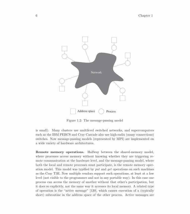
6 Chapter 1
Address space Process
Network
Figure 1.2: The message-passing model
is small). Many clusters use multilevel switched networks, and supercomputers
such as the IBM PERCS and Cray Cascade also use high-radix (many connections)
switches. Now message-passing models (represented by MPI) are implemented on
a wide variety of hardware architectures.
Remote memory operations. Halfway between the shared-memory model,
where processes access memory without knowing whether they are triggering re-
mote communication at the hardware level, and the message-passing model, where
both the local and remote processes must participate, is the remote memory oper-
ation model. This model was typified by put and get operations on such machines
as the Cray T3E. Now multiple vendors support such operations, at least at a low
level (not visible to the programmer and not in any portable way). In this case one
process can access the memory of another without that other’s participation, but
it does so explicitly, not the same way it accesses its local memory. A related type
of operation is the “active message” [120], which causes execution of a (typically
short) subroutine in the address space of the other process. Active messages are

Background 7
often used to facilitate remote memory copying, which can be thought of as part
of the active-message model. Such remote memory copy operations are exactly the
“one-sided” sends and receives unavailable in the classic message-passing model.
The first commercial machine to popularize this model was the TMC CM-5, which
used active messages both directly and as an implementation layer for the TMC
message-passing library.
MPI-style remote memory operations were introduced in the MPI-2 Standard and
further developed in the MPI-3 standard, described in Using Advanced MPI [55].
Hardware support for one-sided operations, even on “commodity” networks, is now
standard. In addition to proprietary interfaces such as IBM’s LAPI [107], there
are industry standards such as InfiniBand [6], which have the potential to bring
good support for remote memory access operations even to inexpensive parallel
computers.
Threads. Early forms of the shared-memory model provided processes with sep-
arate address spaces, which could obtain shared memory through explicit memory
operations, such as special forms of the C malloc operation. The more common
version of the shared-memory model now specifies that all memory be shared. This
allows the model to be applied to multithreaded systems, in which a single pro-
cess (address space) has associated with it several program counters and execution
stacks. Since the model allows fast switching from one thread to another and re-
quires no explicit memory operations, it can be used portably in Fortran programs.
The difficulty imposed by the thread model is that any “state” of the program
defined by the value of program variables is shared by all threads simultaneously,
although in most thread systems it is possible to allocate thread-local memory. One
widely used thread model is specified by the POSIX Standard [76]. A higher-level
approach to programming with threads is also offered by OpenMP [97, 38].
Hybrid models. Combinations of the above models are also possible, in which
some clusters of processes share memory with one another but communicate with
other clusters via message passing (Figure 1.3), or in which single processes may
be multithreaded (separate threads share memory) yet not share memory with one
another. In any case, attached GPUs may contribute vector-style parallelism as
well.
All of the world’s largest parallel machines provide a combined (or hybrid) model
at the hardware level, even though they are currently being programmed largely
with MPI. MPI implementations can take advantage of such hybrid hardware by

8 Chapter 1
Figure 1.3: The hybrid model
utilizing the shared memory to accelerate message-passing operations between pro-
cesses that share memory.
These combined models lead to software complexity, in which a shared-memory
approach (like OpenMP) is combined with a message-passing approach (like MPI),
along with code to manage an attached GPU (like CUDA). A significant number of
applications have been ported to (or originally written for) such complex execution
environments, but at a considerable cost in programming complexity and (in some
cases) loss of portability.
The description of parallel computing models we have given here has focused on
what they look like to the programmer. The underlying hardware for supporting
these and future models continues to evolve. Among these directions is support for
multithreading at the hardware level. One approach has been to add support for
large numbers of threads per processor core; this approach helps hide the relatively
high latency of memory access. The YarcData Urika [16] is the most recent ver-
sion of this approach; previous systems include the Tera MTA and the Denelcor
HEP. Another approach, now used on most commodity processors, is simultaneous
multithreading (sometimes called hyperthreading), where several hardware threads
share the same resources in a compute core. Simultaneous multithreading is usually
transparent to the programmer.

Background 9
1.3.2 Advantages of the Message-Passing Model
In this book we focus on the message-passing model of parallel computation, and
in particular the MPI instantiation of that model. While we do not claim that the
message-passing model is uniformly superior to the other models, we can say here
why it has become widely used and why we can expect it to be around for a long
time.
Universality. The message-passing model fits well on separate processors con-
nected by a (fast or slow) communication network. Thus, it matches the highest
level of the hardware of most of today’s parallel supercomputers, as well as work-
station networks and dedicated PC clusters. Where the machine supplies extra
hardware to support a shared-memory model, the message-passing model can take
advantage of this hardware to speed data transfer. Use of a GPU can be orthogonal
to the use of MPI.
Expressivity. Message passing has been found to be a useful and complete model
in which to express parallel algorithms. It provides the control missing from the
data-parallel and compiler-based models in dealing with data locality. Some find its
anthropomorphic flavor useful in formulating a parallel algorithm. It is well suited
to adaptive, self-scheduling algorithms and to programs that can be made tolerant
of the imbalance in process speeds found on shared networks.
Ease of debugging. Debugging of parallel programs remains a challenging re-
search area. While debuggers for parallel programs are perhaps easier to write for
the shared-memory model, it is arguable that the debugging process itself is eas-
ier in the message-passing paradigm. The reason is that one of the most common
causes of error is unexpected overwriting of memory. The message-passing model,
by controlling memory references more explicitly than any of the other models
(only one process at a time has direct access to any memory location except during
a well-defined, short time period), makes it easier to locate erroneous memory reads
and writes. Some parallel debuggers even can display message queues, which are
normally invisible to the programmer.
Performance. The most compelling reason that message passing will remain a
permanent part of the parallel computing environment is performance. As modern
CPUs have become faster, management of their caches and the memory hierarchy
in general has become the key to getting the most out of these machines. Message
10 Chapter 1
passing provides a way for the programmer to explicitly associate specific data
with processes and thus allow the compiler and cache-management hardware to
function fully. Indeed, one advantage distributed-memory computers have over even
the largest single-processor machines is that they typically provide more memory
and more cache. Memory-bound applications can exhibit superlinear speedups
when ported to such machines. And even on shared-memory computers, use of the
message-passing model can improve performance by providing more programmer
control of data locality in the memory hierarchy.
This analysis explains why message passing has emerged as one of the more widely
used paradigms for expressing parallel algorithms. Although it has shortcomings,
message passing remains closer than any other paradigm to being a standard ap-
proach for the implementation of parallel applications.
1.4 Evolution of Message-Passing Systems
Message passing has only recently, however, become a standard for portability, in
both syntax and semantics. Before MPI, there were many competing variations on
the message-passing theme, and programs could only be ported from one system
to another with difficulty. Several factors contributed to the situation.
Vendors of parallel computing systems, while embracing standard sequential lan-
guages, offered different, proprietary message-passing libraries. There were two
(good) reasons for this situation:
• No standard emerged, and—until MPI—no coherent effort was made to create
one. This situation reflected the fact that parallel computing is a new science,
and experimentation has been needed to identify the most useful concepts.
• Without a standard, vendors quite rightly treated the excellence of their pro-
prietary libraries as a competitive advantage and focused on making their
advantages unique (thus nonportable).
To deal with the portability problem, the research community contributed a
number of libraries to the collection of alternatives. The better known of these
are PICL [52], PVM [27] , PARMACS [29], p4 [31, 35, 36], Chameleon [67], Zip-
code [111], and TCGMSG [68]; these libraries were publicly available but none of
them are still widely used, having been supplanted by MPI. Many other experimen-
tal systems, of varying degrees of portability, have been developed at universities.
In addition, commercial portable message-passing libraries were developed, such
as Express [39], with considerable added functionality. These portability libraries,
Background 11
from the user’s point of view, also competed with one another, and some users were
driven to then write their own metaportable libraries to hide the differences among
them. Unfortunately, the more portable the code thus produced, the less func-
tionality in the libraries the code could exploit, because it must be a least common
denominator of the underlying systems. Thus, to achieve portable syntax, one must
restrict oneself to deficient semantics, and many of the performance advantages of
the nonportable systems are lost.
Sockets, both the Berkeley (Unix) variety and Winsock (Microsoft) variety, also
offer a portable message-passing interface, although with minimal functionality.
We analyze the difference between the socket interface and the MPI interface in
Chapter 9.
1.5 The MPI Forum
The plethora of solutions being offered to the user by both commercial software
makers and researchers eager to give away their advanced ideas for free necessitated
unwelcome choices for the user among portability, performance, and features.
The user community, which definitely includes the software suppliers themselves,
determined to address this problem. In April 1992, the Center for Research in
Parallel Computation sponsored a one-day workshop on Standards for Message
Passing in a Distributed-Memory Environment [121]. The result of that workshop,
which featured presentations of many systems, was a realization both that a great
diversity of good ideas existed among message-passing systems and that people
were eager to cooperate on the definition of a standard.
At the Supercomputing ’92 conference in November, a committee was formed to
define a message-passing standard. At the time of creation, few knew what the
outcome might look like, but the effort was begun with the following goals:
• to define a portable standard for message passing, which would not be an
official, ANSI-like standard but would attract both implementors and users;
• to operate in a completely open way, allowing anyone to join the discussions,
either by attending meetings in person or by monitoring e-mail discussions;
and
• to be finished in one year.
The MPI effort was a lively one, as a result of the tensions among these three
goals. The MPI Forum decided to follow the format used by the High Performance
12 Chapter 1
Fortran Forum, which had been well received by its community. (It even decided
to meet in the same hotel in Dallas.)
The MPI standardization effort has been successful in attracting a wide class
of vendors and users because the MPI Forum itself was so broadly based. At the
original (MPI-1) forum, the parallel computer vendors were represented by Convex,
Cray, IBM, Intel, Meiko, nCUBE, NEC, and Thinking Machines. Members of the
groups associated with the portable software libraries were also present: PVM, p4,
Zipcode, Chameleon, PARMACS, TCGMSG, and Express were all represented.
Moreover, a number of parallel application specialists were on hand. In addition to
meetings every six weeks for more than a year, there were continuous discussions
via electronic mail, in which many persons from the worldwide parallel computing
community participated. Equally important, an early commitment to producing
a model implementation [65] helped demonstrate that an implementation of MPI
was feasible.
The first version of the MPI standard [93] was completed in May 1994. During
the 1993–1995 meetings of the MPI Forum, several issues were postponed in order
to reach early agreement on a core of message-passing functionality. The forum
reconvened during 1995–1997 to extend MPI to include remote memory operations,
parallel I/O, dynamic process management, and a number of features designed to
increase the convenience and robustness of MPI. Although some of the results of
this effort are described in this book, most of them are covered formally in [56] and
described in a more tutorial approach in [60]. We refer to this as MPI-2.
The MPI-2 version remained the definition of MPI for nearly fifteen years. Then,
in response to developments in hardware and software and the needs of applications,
a third instantiation of the forum was constituted, again consisting of vendors, com-
puter scientists, and computational scientists (the application developers). During
2008–2009, the forum updated the MPI-2 functions to reflect recent developments,
culminating in the release of MPI-2.2 in September 2009. The forum continued to
meet, substantially extending MPI with new operations, releasing the MPI-3 stan-
dard in September of 2012. Since then, the forum has continued to meet to further
enhance MPI, for example, considering how MPI should behave in an environment
where hardware is somewhat unreliable.
This book primarily covers the functionality introduced in MPI-1, revised and
updated to reflect the (few) changes that the MPI-2 and MPI-3 forums introduced
into this functionality. It is a companion to the standard itself, showing how MPI
is used and how its features are exploited in a wide range of situations. The more
substantive additions to the MPI-1 standard are covered in the standard itself, of
course, and in Using Advanced MPI [55].

2 Introduction to MPI
In this chapter we introduce the basic concepts of MPI, showing how they arise
naturally out of the message-passing model.
2.1 Goal
The primary goal of the MPI specification is to demonstrate that users need not
compromise among efficiency, portability, and functionality. Specifically, users can
write portable programs that still take advantage of the specialized hardware and
software offered by individual vendors. At the same time, advanced features, such
as application-oriented process structures and dynamically managed process groups
with an extensive set of collective operations, can be expected in every MPI imple-
mentation and can be used in every parallel application program where they might
be useful. One of the most critical families of users is the parallel library writers, for
whom efficient, portable, and highly functional code is extremely important. MPI
is the first specification that allows these users to write truly portable libraries. The
goal of MPI is ambitious; but because the collective effort of collaborative design
and competitive implementation has been successful, it has removed the need for
an alternative to MPI as a means of specifying message-passing algorithms to be
executed on any computer platform that implements the message-passing model.
This tripartite goal—portability, efficiency, functionality—has forced many of the
design decisions that make up the MPI specification. We describe in the following
sections just how these decisions have affected both the fundamental send and
receive operations of the message-passing model and the set of advanced message-
passing operations included in MPI.
2.2 What Is MPI?
MPI is not a revolutionary new way of programming parallel computers. Rather, it
is an attempt to collect the best features of many message-passing systems that have
been developed over the years, improve them where appropriate, and standardize
them. Hence, we begin by summarizing the fundamentals of MPI.
• MPI is a library, not a language. It specifies the names, calling sequences, and
results of subroutines to be called from Fortran programs and the functions
to be called from C programs. The programs that users write in Fortran and
C are compiled with ordinary compilers and linked with the MPI library.

14 Chapter 2
• MPI is a specification, not a particular implementation. As of this writing, all
parallel computer vendors offer an MPI implementation for their machines and
free, publicly available implementations can be downloaded over the Internet.
A correct MPI program should be able to run on all MPI implementations
without change.
• MPI addresses the message-passing model. Although it is far more than a
minimal system, its features do not extend beyond the fundamental compu-
tational model described in Chapter 1. A computation remains a collection
of processes communicating with messages. Functions defined in MPI-2 and
MPI-3 extend the basic message-passing model considerably, but still focus
on the movement of data among separate address spaces.
The structure of MPI makes it straightforward to port existing codes and to write
new ones without learning a new set of fundamental concepts. Nevertheless, the
attempts to remove the shortcomings of prior systems have made even the basic
operations a little different. We explain these differences in the next section.
2.3 Basic MPI Concepts
Perhaps the best way to introduce the basic concepts in MPI is first to derive a
minimal message-passing interface from the message-passing model itself and then
to describe how MPI extends such a minimal interface to make it more useful to
application programmers and library writers.
In the message-passing model of parallel computation, the processes executing
in parallel have separate address spaces. Communication occurs when a portion
of one process’s address space is copied into another process’s address space. This
operation is cooperative and occurs only when the first process executes a send
operations and the second process executes a receive operation. What are the
minimal arguments for the send and receive functions?
For the sender, the obvious arguments that must be specified are the data to be
communicated and the destination process to which the data is to be sent. The
minimal way to describe data is to specify a starting address and a length (in bytes).
Any sort of data item might be used to identify the destination; typically it has
been an integer.
On the receiver’s side, the minimum arguments are the address and length of an
area in local memory where the received variable is to be placed, together with a
variable to be filled in with the identity of the sender, so that the receiving process
can know which process sent it the message.
Introduction to MPI 15
Although an implementation of this minimum interface might be adequate for
some applications, more features usually are needed. One key notion is that of
matching : a process must be able to control which messages it receives, by screening
them by means of another integer, called the type or tag of the message. Since we
are soon going to use “type” for something else altogether, we will use the word
“tag” for this argument to be used for matching. A message-passing system is
expected to supply queuing capabilities so that a receive operation specifying a tag
will complete successfully only when a message sent with a matching tag arrives.
This consideration adds the tag as an argument for both sender and receiver. It is
also convenient if the source can be specified on a receive operation as an additional
screening parameter.
Moreover, it is useful for the receive to specify a maximum message size (for
messages with a given tag) but allow for shorter messages to arrive. In this case
the actual length of the message received needs to be returned in some way.
Now our minimal message interface has become
send(address, length, destination, tag)
and
receive(address, length, source, tag, actlen)
where the source and tag in the receive can be either input arguments used to
screen messages or special values used as “wild cards” to indicate that messages
will be matched from any source or with any tag, in which case they could be
filled in with the actual tag and destination of the message received. The argument
actlen is the length of the message received. Typically it is considered an error
if a matching message is received that is too long, but not if it is too short.
Many systems with variations on this type of interface were in use when the
MPI effort began. Several of them were mentioned in the preceding chapter. Such
message-passing systems proved extremely useful, but they imposed restrictions
considered undesirable by a large user community. The MPI Forum sought to lift
these restrictions by providing more flexible versions of each of these parameters,
while retaining the familiar underlying meanings of the basic send and receive
operations. Let us examine these parameters one by one, in each case discussing
first the original restrictions and then the MPI version.
Describing message buffers. The (address, length) specification of the
message to be sent was a good match for early hardware but is not really adequate
for two different reasons:
16 Chapter 2
• Often, the message to be sent is not contiguous. In the simplest case, it may
be a row of a matrix that is stored columnwise. More generally, it may consist
of an irregularly dispersed collection of structures of different sizes. In the
past, programmers (or libraries) have had to provide code to pack this data
into contiguous buffers before sending it and to unpack it at the receiving
end. However, as communications processors began to appear that could
deal directly with strided or even more generally distributed data, it became
more critical for performance that the packing be done “on the fly” by the
communication processor in order to avoid the extra data movement. This
cannot be done unless the data is described in its original (distributed) form
to the communication library.
• The information content of a message (its integer values, floating-point values,
etc.) is really independent of how these values are represented in a particular
computer as strings of bits. If we describe our messages at a higher level, then
it will be possible to send messages between machines that represent such
values in different ways, such as with different byte orderings or different
floating-point number representations. This will also allow the use of MPI
communication between computation-specialized machines and visualization-
specialized machines, for example, or among workstations of different types
on a network. The communication library can do the necessary conversion if
it is told precisely what is being transmitted.
The MPI solution, for both of these problems, is to specify messages at a higher
level and in a more flexible way than (address, length) in order to reflect the
fact that a message contains much more structure than just a string of bits. Instead,
an MPI message buffer is defined by a triple (address, count, datatype),describing count occurrences of the data type datatype starting at address.The power of this mechanism comes from the flexibility in the values of datatype.To begin with, datatype can take on the values of elementary data types in
the host language. Thus (A, 300, MPI_REAL) describes a vector A of 300 real
numbers in Fortran, regardless of the length or format of a floating-point number.
An MPI implementation for heterogeneous networks guarantees that the same 300
reals will be received, even if the receiving machine has a very different floating-point
format.
The full power of data types, however, comes from the fact that users can con-
struct their own data types using MPI routines and that these data types can
describe noncontiguous data. Details of how to construct these “derived” data
types are given in Chapter 5.
Introduction to MPI 17
Separating families of messages. Nearly all message-passing systems have pro-
vided a tag argument for the send and receive operations. This argument allows
the programmer to deal with the arrival of messages in an orderly way, even if the
arrival of messages is not in the order anticipated. The message-passing system
queues messages that arrive “of the wrong tag” until the program(mer) is ready for
them. Usually a facility exists for specifying wild-card tags that match any tag.
This mechanism has proven necessary but insufficient, because the arbitrariness
of the tag choices means that the entire program must use tags in a predefined,
coherent way. Particular difficulties arise in the case of libraries, written far from the
application programmer in time and space, whose messages must not be accidentally
received by the application program.
MPI’s solution is to extend the notion of tag with a new concept: the context.
Contexts are allocated at run time by the system in response to user (and library)
requests and are used for matching messages. They differ from tags in that they are
allocated by the system instead of the user and no wild-card matching is permitted.
The usual notion of message tag, with wild-card matching, is retained in MPI.
Naming processes. Processes belong to groups. If a group contains n processes,
then its processes are identified within the group by ranks, which are integers from
0 to n − 1. All processes in an MPI implementation belong to an initial group.
Within this group, processes are numbered similarly to the way in which they are
numbered in many previous message-passing systems, from 0 up to 1 less than the
total number of processes.
Communicators. The notions of context and group are combined in a single
object called a communicator, which becomes an argument to most point-to-point
and collective operations. Thus the destination or source specified in a send
or receive operation always refers to the rank of the process in the group identified
with the given communicator.
That is, in MPI the basic (blocking) send operation has become
MPI_Send(address, count, datatype, destination, tag, comm)
where
• (address, count, datatype) describes count occurrences of items of
the form datatype starting at address,
• destination is the rank of the destination in the group associated with the
communicator comm,

18 Chapter 2
• tag is an integer used for message matching, and
• comm identifies a group of processes and a communication context.
The receive has become
MPI_Recv(address, maxcount, datatype, source, tag, comm, status)
Here, the arguments are as follows:
• (address, maxcount, datatype) describe the receive buffer as they do
in the case of MPI_Send. It is allowable for less than maxcount occurrences
of datatype to be received. The arguments tag and comm are as in MPI_-Send, with the addition that a wildcard, matching any tag, is allowed.
• source is the rank of the source of the message in the group associated with
the communicator comm, or a wildcard matching any source,
• status holds information about the actual message size, source, and tag,
useful when wild cards have been used.
The source, tag, and count of the message actually received can be retrieved from
status.Several early message-passing systems returned the “status” parameters by sep-
arate calls that implicitly referenced the most recent message received. MPI’s
method is one aspect of its effort to be reliable in the situation where multiple
threads are receiving messages on behalf of a process.
2.4 Other Interesting Features of MPI
Our focus so far has been on the basic send and receive operations, since one may
well regard as the most fundamental new feature in MPI the small but important
way in which each of the arguments of the “traditional” send/receive was modified
from the minimal message-passing interface we described at the beginning of this
section. Nevertheless, MPI is a large specification and offers many other advanced
features, including the following:
Collective communications. A proven concept from early message-passing li-
braries is the notion of collective operation, performed by all the processes in a
computation. Collective operations are of two kinds:
Introduction to MPI 19
• Data movement operations are used to rearrange data among the processes.
The simplest of these is a broadcast, but many elaborate scattering and gath-
ering operations can be defined (and are supported in MPI).
• Collective computation operations (minimum, maximum, sum, logical OR,
etc., as well as user-defined operations).
In both cases, a message-passing library can take advantage of its knowledge of the
structure of the machine in order to optimize and increase the parallelism in these
operations.
MPI has an extremely flexible mechanism for describing data movement rou-
tines. These are particularly powerful when used in conjunction with the derived
datatypes.
MPI also has a large set of collective computation operations and a mechanism
by which users can provide their own. In addition, MPI provides operations for
creating and managing groups in a scalable way. Such groups can be used to
control the scope of collective operations.
Virtual topologies. One can conceptualize processes in an application-oriented
topology, for convenience in programming. Both general graphs and grids of pro-
cesses are supported in MPI. Topologies provide a high-level method for managing
process groups without dealing with them directly. Since topologies are a standard
part of MPI, we do not treat them as an exotic, advanced feature. We use them
early in the book (Chapter 4) and freely from then on.
Debugging and profiling. Rather than specifying any particular interface, MPI
requires the availability of “hooks” that allow users to intercept MPI calls and thus
define their own debugging and profiling mechanisms. In Chapter 7 we give an
example of how to write such hooks for analyzing program behavior.
Communication modes. MPI has both the blocking send and receive opera-
tions described above and nonblocking versions whose completion can be tested
for and waited for explicitly. It is possible to test and wait on multiple operations
simultaneously. MPI also has multiple communication modes. The standard mode
corresponds to current common practice in message-passing systems. The syn-
chronous mode requires sends to block until the corresponding receive has occurred
(as opposed to the standard mode blocking send, which blocks only until the buffer
can be reused). The ready mode (for sends) is a way for the programmer to notify
20 Chapter 2
the system that the receive has been posted, so that the underlying system can
use a faster protocol if it is available. The buffered mode provides user-controllable
buffering for send operations.
Support for libraries. The structuring of all communication through communi-
cators provides to library writers for the first time the capabilities they need to write
parallel libraries that are completely independent of user code and inter-operable
with other libraries. Libraries can maintain arbitrary data, called attributes, as-
sociated with the communicators they allocate, and can specify their own error
handlers. The tools for creating MPI parallel libraries that take advantage of these
features are described in Chapters 6 and 7.
Support for heterogeneous networks. MPI programs can run on networks of
machines that have different lengths and formats for various fundamental datatypes,
since each communication operation specifies a (possibly very simple) structure and
all the component datatypes, so that the implementation always has enough infor-
mation to do data format conversions if they are necessary. MPI does not specify
how these conversions are done, however, thus allowing a variety of optimizations.
We discuss heterogeneity specifically in Chapter 7.
Processes and processors. The MPI standard talks about processes. A process
is a software concept that represents an address space and one or more threads (each
thread has a separate program counter and call stack). In contrast, a processor
is a piece of hardware containing a central processing unit capable of executing
a program. Some MPI implementations will limit an MPI program to one MPI
process per processor; others will allow multiple MPI processes on each processor.
An MPI process is usually the same as a process in the operating system, but
that isn’t required by the MPI standard. See [41, 78] for examples of one Unix
process containing multiple MPI processes.
2.5 Is MPI Large or Small?
Perhaps the most fundamental decision for the MPI Forum was whether MPI would
be “small and exclusive,” incorporating the minimal intersection of existing li-
braries, or “large and inclusive,” incorporating the union of the functionality of
existing systems.
In the end, although some ideas were left out, an attempt was made to include a
relatively large number of features that had proven useful in various libraries and

Introduction to MPI 21
MPI_Init Initialize MPIMPI_Comm_size Find out how many processes there areMPI_Comm_rank Find out which process I amMPI_Send Send a messageMPI_Recv Receive a messageMPI_Finalize Terminate MPI
Table 2.1: The six-function version of MPI
applications. At the same time the number of ideas in MPI is small; the number
of functions in MPI comes from combining a small set of orthogonal concepts.
To demonstrate just how little one needs to learn to write MPI programs, we
present here a list of the indispensable functions, the ones that the programmer
really cannot do without. There are six. With only these functions a vast number
of useful and efficient programs can be written. The other functions add flexibil-
ity (datatypes), robustness (nonblocking send/receive), efficiency (“ready” mode),
modularity (groups, communicators), or convenience (collective operations, topolo-
gies). Nonetheless, one can forego all of these concepts and use only the six routines
from MPI shown in Table 2.1 to write complete message-passing programs.
The designers of MPI attempted to make the features of MPI consistent and
orthogonal. Hence users can incrementally add sets of functions to their repertoire
as needed, without learning everything at once. For example, for collective com-
munication, one can accomplish a lot with just MPI_Bcast and MPI_Reduce, aswe show in Chapter 3. The next addition to one’s repertoire is likely to be the non-
blocking operations, which we discuss in Chapter 4, followed by derived datatypes,
introduced in Chapter 4 and explored in more depth in Chapter 5. The unfolding
of topics in this book will be driven by examples that motivate the introduction of
MPI routines a little at a time.
2.6 Decisions Left to the Implementor
The MPI standard does not specify every aspect of a parallel program. Some
aspects of parallel programming that are left to the specific implementation are as
follows:
• Process startup is left to the implementation. This strategy allows consider-
able flexibility in how an MPI program is executed, at some cost in portability
of the parallel programming environment.
22 Chapter 2
• Although MPI specifies a number of error codes, the implementation is al-
lowed to return a richer set of error codes than is specified in the standard.
• The amount of system buffering provided for messages is implementation
dependent, although users can exert some control if they choose. In Chapter 4
we describe what we mean by buffering and techniques for dealing with the
buffering problem . Chapter 8 contains a look at buffering issues from the
implementor’s point of view.
• Further issues, including some impacting performance, that come up when
one looks more deeply into implementation issues are covered in Chapter 8.
The implementation used in preparing examples for this book is MPICH [59], a
freely available, portable implementation of MPI. Instructions for obtaining MPICH
and the source code for the examples used here are given in Appendix B.
3 Using MPI in Simple Programs
In this chapter we introduce the most basic MPI calls and use them to write some
simple parallel programs. Simplicity of a parallel algorithm does not limit its use-
fulness, however: even a small number of basic routines are enough to implement a
major application. We also demonstrate in this chapter a few of the tools that we
use throughout this book to study the behavior of parallel programs.
3.1 A First MPI Program
For our first parallel program, we choose a “perfect” parallel program: it can be
expressed with a minimum of communication, load balancing is automatic, and
we can verify the answer. Specifically, we compute the value of π by numerical
integration. Since
∫ 1
0
1
1 + x2dx = arctan(x)|10 = arctan(1)− arctan(0) = arctan(1) =
π
4,
we will integrate the function f(x) = 4/(1+x2). To do this integration numerically,
we divide the interval from 0 to 1 into some number n of subintervals and add up
the areas of the rectangles as shown in Figure 3.1 for n = 5. Larger values of the
parameter n will give us more accurate approximations of π. This is not, in fact, a
very good way to compute π, but it makes a good example.
To see the relationship between n and the error in the approximation, we write
an interactive program in which the user supplies n and the program first computes
an approximation (the parallel part of the program) and then compares it with a
known, highly accurate approximation to π.
The parallel part of the algorithm occurs as each process computes and adds up
the areas for a different subset of the rectangles. At the end of the computation,
all of the local sums are combined into a global sum representing the value of π.
Communication requirements are consequently simple. One of the processes (we’ll
call it the manager) is responsible for communication with the user. It obtains a
value for n from the user and broadcasts it to all of the other processes. Each
process is able to compute which rectangles it is responsible for from n, the total
number of processes, and its own rank. After reporting a value for π and the error
in the approximation, the manager asks the user for a new value for n.
The complete program is shown in Figure 3.2. In most of this book we will show
only the “interesting” parts of programs and refer the reader to other sources for
the complete, runnable version of the code. For our first few programs, however,
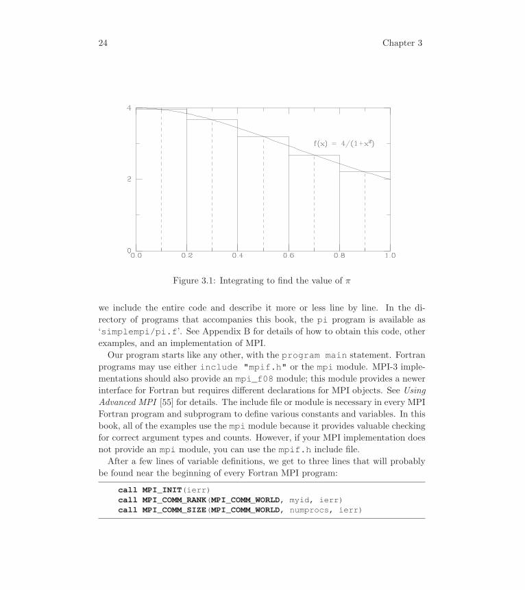
24 Chapter 3
Figure 3.1: Integrating to find the value of π
we include the entire code and describe it more or less line by line. In the di-
rectory of programs that accompanies this book, the pi program is available as
‘simplempi/pi.f’. See Appendix B for details of how to obtain this code, other
examples, and an implementation of MPI.
Our program starts like any other, with the program main statement. Fortran
programs may use either include "mpif.h" or the mpi module. MPI-3 imple-
mentations should also provide an mpi_f08 module; this module provides a newer
interface for Fortran but requires different declarations for MPI objects. See Using
Advanced MPI [55] for details. The include file or module is necessary in every MPI
Fortran program and subprogram to define various constants and variables. In this
book, all of the examples use the mpi module because it provides valuable checking
for correct argument types and counts. However, if your MPI implementation does
not provide an mpi module, you can use the mpif.h include file.
After a few lines of variable definitions, we get to three lines that will probably
be found near the beginning of every Fortran MPI program:
call MPI_INIT(ierr)call MPI_COMM_RANK(MPI_COMM_WORLD, myid, ierr)call MPI_COMM_SIZE(MPI_COMM_WORLD, numprocs, ierr)

Using MPI in Simple Programs 25
program mainuse mpidouble precision PI25DTparameter (PI25DT = 3.141592653589793238462643d0)double precision mypi, pi, h, sum, x, f, ainteger n, myid, numprocs, i, ierr
! function to integratef(a) = 4.d0 / (1.d0 + a*a)
call MPI_INIT(ierr)call MPI_COMM_RANK(MPI_COMM_WORLD, myid, ierr)call MPI_COMM_SIZE(MPI_COMM_WORLD, numprocs, ierr)
doif (myid .eq. 0) then
print *, ’Enter the number of intervals: (0 quits) ’read(*,*) n
endif! broadcast n
call MPI_BCAST(n, 1, MPI_INTEGER, 0, MPI_COMM_WORLD, ierr)! check for quit signal
if (n .le. 0) exit! calculate the interval size
h = 1.0d0/nsum = 0.0d0do i = myid+1, n, numprocs
x = h * (dble(i) - 0.5d0)sum = sum + f(x)
enddomypi = h * sum
! collect all the partial sumscall MPI_REDUCE(mypi, pi, 1, MPI_DOUBLE_PRECISION, &
MPI_SUM, 0, MPI_COMM_WORLD, ierr)! node 0 prints the answer.
if (myid .eq. 0) thenprint *, ’pi is ’, pi, ’ Error is’, abs(pi - PI25DT)
endifenddocall MPI_FINALIZE(ierr)end
Figure 3.2: Fortran program (fpi) for calculating π

26 Chapter 3
The call to MPI_INIT is required in every MPI program and must be the first MPI
call.1 It establishes the MPI “environment.” Only one invocation of MPI_INITcan occur in each program execution. Its only argument is an error code. Every
Fortran MPI subroutine returns an error code in its last argument, which is either
MPI_SUCCESS or an implementation-defined error code. In this example (and in
many of our examples) we will be sloppy and not test the return codes from our
MPI routines, assuming that they will always be MPI_SUCCESS. This approach
will improve readability of the code at the expense of possible debugging time. We
will discuss later (in Section 7.7) how to check, handle, and report errors.
As described in Chapter 2, all MPI communication is associated with a com-
municator that describes the communication context and an associated group of
processes. In this program we will be using only the default communicator, prede-
fined and named MPI_COMM_WORLD, which defines one context and the set of all
processes. MPI_COMM_WORLD is one of the items defined in the mpi module and
in ‘mpif.h’.The call MPI_COMM_SIZE returns (in numprocs) the number of processes that
the user has started for this program. Precisely how the user caused these processes
to be started depends on the implementation, but any program can find out the
number with this call. The value numprocs is actually the size of the group of
processes associated with the default communicator MPI_COMM_WORLD. We think
of the processes in any group as being numbered with consecutive integers beginning
with 0, called ranks. By calling MPI_COMM_RANK, each process finds out its rank
in the group associated with a communicator. Thus, although each process in this
program will get the same number in numprocs, each will have a different number
for myid.Next, the manager process (which can identify itself by using myid) gets a value
for n, the number of rectangles, from the user. The line
call MPI_BCAST(n, 1, MPI_INTEGER, 0, MPI_COMM_WORLD, ierr)
sends the value of n to all other processes. Note that all processes call MPI_BCAST,both the process sending the data (with rank zero) and all of the other processes
in MPI_COMM_WORLD.2 The call to MPI_BCAST results in every process (in the
1There are a few exceptions, including the MPI_Initialized routine, which a library can callto determine whether MPI_Init has been called. See Section 7.8.2.
2In some message-passing systems, messages sent with a broadcast can be received with areceive, just like a message sent with a send. In MPI, communication involving more than twoprocesses is collective, and all participating processes call the same routine. MPI_BCAST is anexample of a collective communication routine.

Using MPI in Simple Programs 27
group associated with the communicator given in the fifth argument) ending up
with a copy of n. The data to be communicated is described by the address (n),the datatype (MPI_INTEGER), and the number of items (1). The process with
the original copy is specified by the fourth argument (0 in this case, the manager
process, which just reads it from the user). (MPI assigns a type to every data item.
MPI datatypes are described in full in Section 5.1.)
Thus, after the call to MPI_BCAST, all processes have n and their own identifiers,
which is enough information for each one to compute its contribution, mypi. Eachprocess computes the area of every numprocs’th rectangle, starting with myid+1.Next, all of the values of mypi held by the individual processes need to be added up.
MPI provides a rich set of such operations, using the MPI_REDUCE routine, with
an argument specifying which arithmetic or logical operation is being requested. In
our case the call is
call MPI_REDUCE(mypi, pi, 1, MPI_DOUBLE_PRECISION, MPI_SUM, 0, &MPI_COMM_WORLD, ierr)
The first two arguments identify the source and result addresses, respectively. The
data being collected consists of 1 (third argument) item of type MPI_DOUBLE_-PRECISION (fourth argument). The operation is addition (MPI_SUM, the next
argument), and the result of the operation is to be placed in pi on the process
with rank 0 (fifth argument). The last two arguments are the communicator and
error return code, as usual. The first two arguments of MPI_REDUCE must not
overlap (i.e., must be different variables or sections of an array). A full list of
such operations is presented in Section 7.2.2, where user-defined operations are
also discussed.
All processes then return to the top of the loop (the manager prints the answer
first). The MPI_BCAST causes all the processes except the manager to wait for the
next value of n.When the user types a zero in response to the request for a number of rectangles,
the loop terminates and all processes execute
call MPI_FINALIZE(ierr)
This call must be made by every process in an MPI computation; it terminates the
MPI “environment.” With few exceptions, no MPI calls may be made by a process
after its call to MPI_FINALIZE. In particular, MPI_INIT cannot be called again.
The Fortran bindings for the MPI routines used in this section are summarized
in Table 3.1. In the tables of Fortran bindings, the expression <type> stands for
any Fortran datatype, such as INTEGER or DOUBLE PRECISION.

28 Chapter 3
MPI INIT(ierror)integer ierror
MPI COMM SIZE(comm, size, ierror)integer comm, size, ierror
MPI COMM RANK(comm, rank, ierror)integer comm, rank, ierror
MPI BCAST(buffer, count, datatype, root, comm, ierror)
<type> buffer(*)integer count, datatype, root, comm, ierror
MPI REDUCE(sendbuf, recvbuf, count, datatype, op, root, comm, ierror)
<type> sendbuf(*), recvbuf(*)integer count, datatype, op, root, comm, ierror
MPI FINALIZE(ierror)integer ierror
Table 3.1: Fortran bindings for routines used in the fpi program
3.2 Running Your First MPI Program
The way in which MPI programs are “launched” on a particular machine or network
is not itself part of the MPI standard. Therefore it may vary from one machine to
another. Several existing MPI implementations have used a syntax like
mpirun -np 4 fpi
The MPI Forum settled on a standard that recommended, but did not require, the
syntax
mpiexec -n 4 fpi
instead. See Using Advanced MPI [55] for a complete discussion of the options for
mpiexec.Some MPI implementations may require different commands to start MPI pro-
grams; often man mpi will give tell you how to run programs. The MPI standard
strongly encourages implementors to provide an mpiexec command that provides
a uniform interface to starting MPI programs.

Using MPI in Simple Programs 29
int MPI Init(int *argc, char ***argv)
int MPI Comm size(MPI Comm comm, int *size)
int MPI Comm rank(MPI Comm comm, int *rank)
int MPI Bcast(void *buf, int count, MPI Datatype datatype, int root,MPI Comm comm)
int MPI Reduce(const void *sendbuf, void *recvbuf, int count,MPI Datatype datatype, MPI Op op, int root, MPI Comm comm)
int MPI Finalize()
Table 3.2: C bindings for routines used in the pi program
3.3 A First MPI Program in C
In this section we repeat the program for computing the value of π, but this time
in C rather than Fortran. In general, every effort was made in MPI to keep the
Fortran and C bindings similar. The primary difference is that error codes are
returned as the value of C functions instead of in a separate argument. In addition,
the arguments to most functions are more strongly typed than they are in Fortran
(with the mpi module), having specific C types such as MPI_Comm and MPI_-Datatype where Fortran has integers (the mpi_f08 Fortran module provides
similarly strong typing). The included file is, of course, different: instead of the mpimodule, we #include the file ‘mpi.h’. Moreover, the arguments to MPI_Init are
different, so that a C program can take advantage of command-line arguments. An
MPI implementation is expected to remove from the argv array any command-line
arguments that should be processed by the implementation before returning control
to the user program and to decrement argc accordingly. Note that the arguments
to MPI_Init in C are the addresses of the usual main arguments argc and argv.One is allowed to pass NULL for both of these addresses.
The program is shown in Figure 3.3, and definitions of the C versions of the MPI
routines used in this program are given in Table 3.2.
3.4 Using MPI from Other Languages
The current MPI standard (version 3.0 at the time of this writing) defines language
bindings for Fortran and C. At one point explicit C++ bindings were defined as

30 Chapter 3
#include "mpi.h"#include <math.h>int main(int argc, char *argv[]){
int n, myid, numprocs, i;double PI25DT = 3.141592653589793238462643;double mypi, pi, h, sum, x;MPI_Init(&argc,&argv);MPI_Comm_size(MPI_COMM_WORLD, &numprocs);MPI_Comm_rank(MPI_COMM_WORLD, &myid);while (1) {
if (myid == 0) {printf("Enter the number of intervals: (0 quits) ");scanf("%d",&n);
}MPI_Bcast(&n, 1, MPI_INT, 0, MPI_COMM_WORLD);if (n == 0)
break;else {
h = 1.0 / (double) n;sum = 0.0;for (i = myid + 1; i <= n; i += numprocs) {
x = h * ((double)i - 0.5);sum += (4.0 / (1.0 + x*x));
}mypi = h * sum;MPI_Reduce(&mypi, &pi, 1, MPI_DOUBLE, MPI_SUM, 0,
MPI_COMM_WORLD);if (myid == 0)
printf("pi is approximately %.16f, Error is %.16f\n",pi, fabs(pi - PI25DT));
}}MPI_Finalize();return 0;
}
Figure 3.3: C program for calculating π
Using MPI in Simple Programs 31
well (see the second edition of this book); but they did not prove useful in the long
run and so have been removed from the standard. C++ users should be able to
freely use the C bindings by including into their program the file ‘mpi.h’, whichdefines them. Individual computer scientists have produced bindings for other
languages, although they are not officially blessed by the MPI Forum and may not
be complete. A web search will turn up at least experimental bindings for languages
such as Python, Ruby, Java, Julia, and D.
3.5 Timing MPI Programs
Sequential algorithms are tested for correctness by seeing whether they give the
right answer. For parallel programs, the right answer is not enough: one wishes
to decrease the execution time. Therefore, measuring speed of execution is part of
testing the program to see whether it performs as intended.
Many operating systems and libraries provide timing mechanisms, but so far all
of those that both are portable and provide access to high resolution clocks are
cumbersome to use. Therefore MPI provides a simple routine that can be used to
time programs or sections of programs.
MPI_Wtime() returns a double-precision floating-point number that is the time
in seconds since some arbitrary point of time in the past. The point is guaran-
teed not to change during the lifetime of a process. Thus, a time interval can be
measured by calling this routine at the beginning and end of a program segment
and subtracting the values returned. Making this a floating-point value allows the
use of high-resolution timers if they are supported by the underlying hardware,
although no particular resolution is specified. MPI provides a function to find out
what the resolution is. This function, called MPI_Wtick, has no arguments. It
returns a floating-point number that is the time in seconds between successive ticks
of the clock. The bindings are shown in Tables 3.3 and 3.4. The values returned
by MPI_Wtime are not synchronized with other processes. That is, you cannot
compare a value from MPI_Wtime from process 8 with a value from process 2.
Only the difference in values of MPI_Wtime, taken on the same process, has any
meaning.3
Suppose we wished to measure the speedup obtained by our program for com-
puting π. Since this program is written as an interactive program, we wish to time
only the section that does internal communications and computation. We don’t
3If in fact the values of MPI_Wtime are synchronized among the processes, the MPI implemen-tation sets an attribute to indicate this. This will be discussed in Section 7.8.
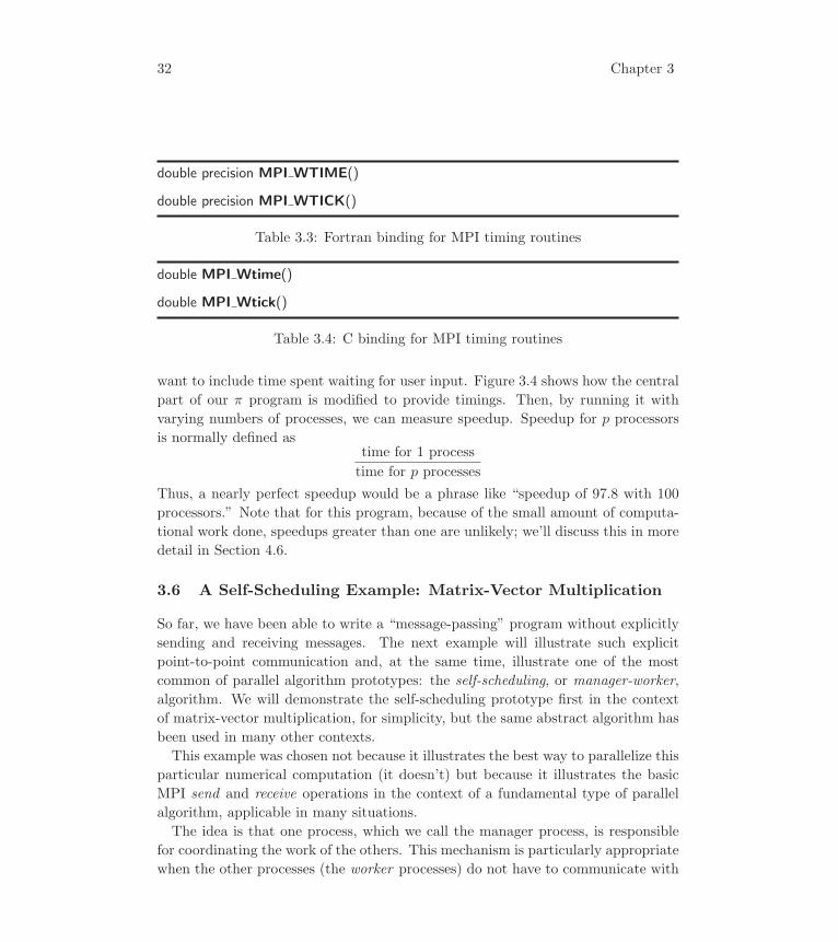
32 Chapter 3
double precision MPI WTIME()
double precision MPI WTICK()
Table 3.3: Fortran binding for MPI timing routines
double MPI Wtime()
double MPI Wtick()
Table 3.4: C binding for MPI timing routines
want to include time spent waiting for user input. Figure 3.4 shows how the central
part of our π program is modified to provide timings. Then, by running it with
varying numbers of processes, we can measure speedup. Speedup for p processors
is normally defined astime for 1 process
time for p processes
Thus, a nearly perfect speedup would be a phrase like “speedup of 97.8 with 100
processors.” Note that for this program, because of the small amount of computa-
tional work done, speedups greater than one are unlikely; we’ll discuss this in more
detail in Section 4.6.
3.6 A Self-Scheduling Example: Matrix-Vector Multiplication
So far, we have been able to write a “message-passing” program without explicitly
sending and receiving messages. The next example will illustrate such explicit
point-to-point communication and, at the same time, illustrate one of the most
common of parallel algorithm prototypes: the self-scheduling, or manager-worker,
algorithm. We will demonstrate the self-scheduling prototype first in the context
of matrix-vector multiplication, for simplicity, but the same abstract algorithm has
been used in many other contexts.
This example was chosen not because it illustrates the best way to parallelize this
particular numerical computation (it doesn’t) but because it illustrates the basic
MPI send and receive operations in the context of a fundamental type of parallel
algorithm, applicable in many situations.
The idea is that one process, which we call the manager process, is responsible
for coordinating the work of the others. This mechanism is particularly appropriate
when the other processes (the worker processes) do not have to communicate with

Using MPI in Simple Programs 33
double precision starttime, endtime...do
! ... read n on process zerostarttime = MPI_WTIME()
! broadcast ncall MPI_BCAST(n, 1, MPI_INTEGER, 0, MPI_COMM_WORLD, ierr)
! check for quit signalif ( n .le. 0 ) exit
! calculate the interval sizeh = 1.0d0/nsum = 0.0d0do i = myid+1, n, numprocs
x = h * (dble(i) - 0.5d0)sum = sum + f(x)
enddomypi = h * sum
! collect all the partial sumscall MPI_REDUCE(mypi, pi, 1, MPI_DOUBLE_PRECISION, &
MPI_SUM, 0, MPI_COMM_WORLD, ierr)! node 0 prints the answer.
endtime = MPI_WTIME()if (myid .eq. 0) then
print *, ’pi is ’, pi, ’Error is ’, abs(pi - PI25DT)print *, ’time is ’, endtime-starttime, ’ seconds’
endifenddo
Figure 3.4: Timing the program for calculating π
one another and when the amount of work that each worker must perform is difficult
to predict. In the case of matrix-vector multiplication, the first criterion holds but
not the second. We can, of course, take the view that we might be computing on a
network of workstations with varying loads and so, even if equal amounts of work
were assigned, the time it takes for each worker to complete its task might vary
widely. In any event, the point of this example is the use of the MPI send and
receive routines to express the manager-worker parallel algorithm, rather than the
matrix-vector multiplication itself.
In our example of multiplying a matrix by a vector, a unit of work to be given
out will consist of the dot product of one row of the matrix A with the (column)
vector b. The manager begins by broadcasting b to each worker. It then sends
34 Chapter 3
one row of the matrix A to each worker. At this point the manager begins a loop,
terminated when it has received all of the entries in the product. The body of the
loop consists of receiving one entry in the product vector from whichever worker
sends one, then sending the next task to that worker. In other words, completion
of one task by a worker is considered to be a request for the next task. Once all
tasks have been handed out, termination messages are sent instead.
Each worker, after receiving the broadcast value of b, also enters a loop, ter-
minated by the receipt of the termination message from the manager. The body
of the loop consists of receiving a row of A, forming the dot product with b, and
sending the answer back to the manager.
Although the manager and workers execute distinct algorithms, and in some
environments they can be compiled into separate executable files, the more portable
and convenient alternative is to combine them into a single program, with a test
near the beginning to separate the manager code from the worker code.
We present the code here in three chunks: the code executed by all processes, the
code executed only by the manager, and the code executed only by the workers.
The code that is executed by all processes is shown in Figure 3.5. It does not
contain any MPI calls that we have not already seen.
Now we fill in the sections carried out by the manager and workers. The way in
which the manager obtains the matrix A and the vector b is irrelevant, so we don’t
show their initialization here. We have arbitrarily made A of size 100 × 100, just
to be specific. The code for the manager is shown in Figure 3.6 on page 37. The
new MPI call is the send operation, which the manager uses to send a row of A
to a worker. In this first version we pack the data into a contiguous buffer before
sending it. (In Section 5.2, we will show how MPI can do this for us.) Then the
message is sent to process i with
tag = idest = icall MPI_SEND(buffer, cols, MPI_DOUBLE_PRECISION, dest, &
tag, MPI_COMM_WORLD, ierr)
The first three arguments, buffer, cols, and MPI_DOUBLE_PRECISION, de-scribe the message in the usual MPI way: address, count, and datatype. The next
argument, i, is the destination, an integer specifying the rank of the destination
process in the group associated with the communicator given by the argument
MPI_COMM_WORLD. Next comes an integer message type, or tag, in MPI terminol-
ogy. We use the tag in this case to send a little extra information along with the
row, namely, the row number. The worker will send this number back with the

Using MPI in Simple Programs 35
program mainuse mpiinteger MAX_ROWS, MAX_COLS, rows, colsparameter (MAX_ROWS = 1000, MAX_COLS = 1000)double precision a(MAX_ROWS,MAX_COLS), b(MAX_COLS)double precision c(MAX_ROWS), buffer(MAX_COLS), ans
integer myid, manager, numprocs, ierr, status(MPI_STATUS_SIZE)integer i, j, numsent, senderinteger anstype, row
call MPI_INIT(ierr)call MPI_COMM_RANK(MPI_COMM_WORLD, myid, ierr)call MPI_COMM_SIZE(MPI_COMM_WORLD, numprocs, ierr)manager = 0rows = 100cols = 100
if (myid .eq. manager) then! manager initializes and then dispatches
...else
! workers receive b, then compute dot products until they! receive a done message
...endif
call MPI_FINALIZE(ierr)end
Figure 3.5: Fortran program for matrix-vector multiplication: common part

36 Chapter 3
dot product it computes, so the manager will know where to store the answer in
the vector c. Of course, we are assuming that there are enough tag values to keep
track of the rows of A. MPI guarantees that at least the values from 0 to 32767
are valid, which will suffice for small tests of this program. (More tag values might
be available; see Section 7.8 for how to find out. We reserve tag value 0 for the
termination message. Then a communicator is specified (in this case the “default”
communicator MPI_COMM_WORLD, whose group includes all processes), and a place
(ierr) in which to return an error code. (We will consider error codes in more
detail in Section 7.7.)
The responses from the workers are received by the line
call MPI_RECV(ans, 1, MPI_DOUBLE_PRECISION, MPI_ANY_SOURCE, &MPI_ANY_TAG, MPI_COMM_WORLD, status, ierr)
This is a blocking receive; that is, control is not returned to the user program until
the message has been received. The first three arguments specify a place to put
the message. Here it is a single double-precision number, the dot product of one
row of A with b. The manager process can also specify that it wishes to wait for a
message from a specific process. Here it does not wish to be so selective, so it uses
the predefined value MPI_ANY_SOURCE to indicate that it will accept messages
from any process associated with the MPI_COMM_WORLD communicator. The use
of MPI ANY TAG indicates that any row is acceptable.
The argument status is an output argument that provides information about
the message that is received (including the source, tag, and length). In Fortran,
it is an array of integers of size MPI_STATUS_SIZE. It is declared in the user’s
program. Here we have called it status. The entry status(MPI_SOURCE) is
filled in with the rank of the process that sent the message. It is important here
because we will send the next unit of work (the next row) to that worker. We also
need to know the value of status(MPI_TAG) in order to know where to store
the answer in the vector c. In C, status is a structure of type MPI_Status; theelement status.MPI_SOURCE is the source, and the element status.MPI_TAGis the tag value. In C programs, the status is usually passed by reference (that is,
&status). In Fortran and C, other entries in status are used to determine the
number of items that were actually received with the routine MPI_Get_count,which we will discuss in Section 7.1.3.
After all rows have been sent, the manager sends a message with tag zero to the
workers to tell them they are finished. The content of this message is irrelevant; all
the information is carried by the tag. In fact, since the content of the message is
irrelevant, we send a message of zero length by setting the count field to zero.

Using MPI in Simple Programs 37
! manager initializes and then dispatches! initialize a and b (arbitrary)
do j = 1,colsb(j) = 1do i = 1,rows
a(i,j) = ienddo
enddonumsent = 0
! send b to each worker processcall MPI_BCAST(b, cols, MPI_DOUBLE_PRECISION, manager, &
MPI_COMM_WORLD, ierr)! send a row to each worker process; tag with row number
do i = 1,min(numprocs-1,rows)do j = 1,cols
buffer(j) = a(i,j)enddocall MPI_SEND(buffer, cols, MPI_DOUBLE_PRECISION, i, &
i, MPI_COMM_WORLD, ierr)numsent = numsent+1
enddodo i = 1,rows
call MPI_RECV(ans, 1, MPI_DOUBLE_PRECISION, &MPI_ANY_SOURCE, MPI_ANY_TAG, &MPI_COMM_WORLD, status, ierr)
sender = status(MPI_SOURCE)anstype = status(MPI_TAG) ! row is tag valuec(anstype) = ansif (numsent .lt. rows) then ! send another row
do j = 1,colsbuffer(j) = a(numsent+1,j)
enddocall MPI_SEND(buffer, cols, MPI_DOUBLE_PRECISION, &
sender, numsent+1, MPI_COMM_WORLD, ierr)numsent = numsent+1
else ! Tell sender that there is no more workcall MPI_SEND(MPI_BOTTOM, 0, MPI_DOUBLE_PRECISION, &
sender, 0, MPI_COMM_WORLD, ierr)endif
enddo
Figure 3.6: Fortran program for matrix-vector multiplication: manager part
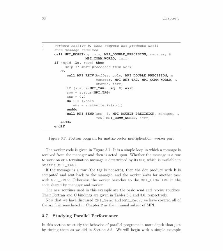
38 Chapter 3
! workers receive b, then compute dot products until! done message received
call MPI_BCAST(b, cols, MPI_DOUBLE_PRECISION, manager, &MPI_COMM_WORLD, ierr)
if (myid .le. rows) then! skip if more processes than workdo
call MPI_RECV(buffer, cols, MPI_DOUBLE_PRECISION, &manager, MPI_ANY_TAG, MPI_COMM_WORLD, &status, ierr)
if (status(MPI_TAG) .eq. 0) exitrow = status(MPI_TAG)ans = 0.0do i = 1,cols
ans = ans+buffer(i)*b(i)enddocall MPI_SEND(ans, 1, MPI_DOUBLE_PRECISION, manager, &
row, MPI_COMM_WORLD, ierr)enddo
endif
Figure 3.7: Fortran program for matrix-vector multiplication: worker part
The worker code is given in Figure 3.7. It is a simple loop in which a message is
received from the manager and then is acted upon. Whether the message is a row
to work on or a termination message is determined by its tag, which is available in
status(MPI_TAG).If the message is a row (the tag is nonzero), then the dot product with b is
computed and sent back to the manager, and the worker waits for another task
with MPI_RECV. Otherwise the worker branches to the MPI_FINALIZE in the
code shared by manager and worker.
The new routines used in this example are the basic send and receive routines.
Their Fortran and C bindings are given in Tables 3.5 and 3.6, respectively.
Now that we have discussed MPI_Send and MPI_Recv, we have covered all of
the six functions listed in Chapter 2 as the minimal subset of MPI.
3.7 Studying Parallel Performance
In this section we study the behavior of parallel programs in more depth than just
by timing them as we did in Section 3.5. We will begin with a simple example

Using MPI in Simple Programs 39
MPI SEND(buf, count, datatype, dest, tag, comm, ierror)
<type> buf(*)integer count, datatype, dest, tag, comm, ierror
MPI RECV(buf, count, datatype, source, tag, comm, status, ierror)
<type> buf(*)integer count, datatype, source, tag, comm,
status(MPI STATUS SIZE), ierror
Table 3.5: Fortran bindings for send and receive routines
int MPI Send(const void *buf, int count, MPI Datatype datatype, int dest, int tag,MPI Comm comm)
int MPI Recv(void *buf, int count, MPI Datatype datatype, int source, int tag,
MPI Comm comm, MPI Status *status)
Table 3.6: C bindings for send and receive routines
of scalability analysis, applied to matrix-vector and matrix-matrix multiplication.
This is an interesting and deep topic in its own right (see, for example, [49] or [80]).
We can convey the flavor of an analysis by looking at the program we have just
written. We will then switch from an analytical approach to an experimental one
and show how to instrument a program so that it produces a log that we can study
with graphical tools.
3.7.1 Elementary Scalability Calculations
Scalability analysis is the estimation of the computation and communication re-
quirements of a particular problem and the mathematical study of how these re-
quirements change as the problem size and/or the number of processes changes. As
an elementary example, let us look at the matrix-vector multiplication algorithm
that we have just presented. The amount of computation is easy to estimate. Let
us suppose, for simplicity, that the matrix A is square, of size n×n. Then for each
element of the product c of A and b, we have to perform n multiplications and
n − 1 additions. There are n elements of c, so the total number of floating-point
operations is
n× (n+ (n− 1)) = 2n2 − n.
40 Chapter 3
For simplicity, we assume that additions and multiplications take the same amount
of time, which we call Tcalc. We assume further that the total computation time is
dominated by the floating-point operations. Thus our rough estimate for compu-
tation time is (2n2 − n)× Tcalc.
Now let us estimate the communication costs. Let us not count the cost of
sending b to each worker process, assuming that it arrived there some other way
(perhaps it is computed there). Then the number of floating-point numbers that
have to be communicated is n (to send a row of A), + 1 (to send the answer back)
for each element of c, for a grand total of
n× (n+ 1) = n2 + n.
If we assume that the time it takes to communicate a floating-point number is
Tcomm, the total communication time is roughly (n2 + n)× Tcomm.
Therefore the ratio of communication to computation is
(n2 + n
2n2 − n
)×
(Tcomm
Tcalc
).
Since the cost of a single floating-point operation is usually much less than the cost
of communicating one floating-point number, we hope to make this ratio as small
as possible. Often by making a problem larger, one can reduce to insignificance
the communication overhead. Here the bad news is that it doesn’t happen in this
case. The ratio Tcomm/Tcalc is roughly independent of n. (For the purposes of this
analysis, we will ignore the effects of message sizes on communication costs; more
detail is presented in Section 4.6.) As n gets larger, the ratio n2+n2n2−n just gets closer
to 12 . This means that communications overhead will always be a problem in this
simplistic algorithm for matrix-vector multiply. (In Chapter 4, we will discuss the
effect of message size on the communication cost.)
Better news is provided by a similar analysis of matrix-matrix multiplication.
We can easily modify our matrix-vector algorithm to multiply two matrices instead.
The vector b becomes a matrix B, we still distribute a copy of B to all the worker
processes, and we collect back a whole row of the product matrix C from each
process. The worker code is shown in Figure 3.8, and the manager code is modified
accordingly. (We save listing of the whole program until later, when we show the
instrumented version.)
Now let us do the scalability analysis for this (still not so very good) algorithm
for matrix multiplication. For simplicity, let us again suppose that A is square and
that B is square as well. Then the number of operations for each element of C is

Using MPI in Simple Programs 41
! workers receive B, then compute rows of C until done messagedo i = 1,bcols
call MPI_BCAST(b(1,i), brows, MPI_DOUBLE_PRECISION, &manager, MPI_COMM_WORLD, ierr)
enddodo
call MPI_RECV(buffer, acols, MPI_DOUBLE_PRECISION, manager,&MPI_ANY_TAG, MPI_COMM_WORLD, status, ierr)
if (status(MPI_TAG) .eq. 0) exitrow = status(MPI_TAG)do i = 1,bcols
ans(i) = 0.0do j = 1,acols
ans(i) = ans(i) + buffer(j)*b(j,i)enddo
enddocall MPI_SEND(ans, bcols, MPI_DOUBLE_PRECISION, manager, &
row, MPI_COMM_WORLD, ierr)enddo
Figure 3.8: Matrix-matrix multiplication: worker part
(as before) n multiplications and n−1 adds, but now there are n2 elements of C to
be computed, as opposed to n. Therefore, the number of floating-point operations
is
n2 × (2n− 1) = 2n3 − n2.
The number of floating-point numbers communicated for each row is n (to send the
row of A, plus n to send the row of C back), and there are n rows, so
n× 2n
is the answer. Now the ratio of communication to computation is(2n2
2n3 − n2
)×
(Tcomm
Tcalc
),
which approaches 1/n as n becomes large. Therefore for this problem we should
expect communication overhead to play a smaller role than in large problems.
3.7.2 Gathering Data on Program Execution
Timing results provide some insight into the performance of our program, and our
programs so far have not been difficult to understand. But suppose that we need
42 Chapter 3
to see in detail just what the sequence of events was, just what amounts of time
were spent on each phase of the computation, and just how long each individual
communication operation took. The easiest way to understand this data at a glance
would be through a graphical tool of some kind.
Several projects have been developed to create files of events with associated
time stamps and then examine them in postmortem fashion by interpreting them
graphically on a workstation. Such files are called logfiles.
In this book we will use some simple tools for creating logfiles and viewing them.
We treat the library for creation of logfiles as separate from the message-passing
library. Viewing the logfile is independent of its creation, and multiple tools can
be used. The tools we describe in this chapter are the ones we used to prepare
the illustrative screenshots shown here. They are part of the MPE (MultiPro-
cessing Environment) described more fully in AppendixA. Since MPE was initially
developed, other tools, similar in intent, have been developed and made widely
available. See, for example, [10, 99, 108]. Although these systems have different
interfaces and capabilities, they are used in similar ways, so our discussion of MPE
remains a useful guide to using them for performance analysis.
In the next few sections we describe routines in the MPE library for explicit log-
ging of programmer-chosen events under program control, and we use the matrix-
matrix multiplication program as an example. These routines will be used in Chap-
ter 7 to build a completely automatic logging mechanism based on the standard
MPI profiling interface.
The logfile viewing program we demonstrate here is called upshot; it is a sim-
ple graphical display of parallel time lines and state durations, based on an ear-
lier program of the same name [70]. Further description of upshot is given in
Appendix A.4 Upshot itself has evolved into a newer graphical display system,
written in Java in Chicago during the era of Michael Jordan and therefore called
Jumpshot [129]. The logging systems cited above all use a form of it for displaying
logfiles.
3.7.3 Instrumenting a Parallel Program with MPE Logging
Although there are advantages to having logfile creation and logfile examination
be parts of a single integrated system, we separate them so that they can undergo
separate development. We present in this section the MPE library for logfile cre-
4The strange name “upshot” arose historically. Once there was a program called “gist” thatwas written at BBN for the Butterfly software environment. It inspired a program written atArgonne, and the thesaurus suggested “upshot” as related to “gist.”
Using MPI in Simple Programs 43
ation. It is designed to coexist with any MPI implementation. It is also used in
the automatic instrumentation techniques for MPI programs discussed in Chap-
ter 7. Reference bindings for MPE are given in Appendix A. Here we describe
the routines needed to instrument a program with explicit, programmer-controlled
events. In Chapter 7 we show how automatic logging can be done, with a decrease
in programmer involvement but a corresponding decrease in flexibility.
Generally speaking, we need to call the MPE_Log_event routine only when
we wish to record a log. The time-stamp and process identifier are collected au-
tomatically; the user specifies an event type and optionally can also supply one
integer data item and one (short) character string. In addition, each process must
call MPE_Init_log to prepare for logging and MPE_Finish_log to merge the
files being stored locally at each process into a single logfile, which is written out.
MPE_Stop_log can be used to suspend logging, although the timer continues to
run. MPE_Start_log causes logging to resume.
3.7.4 Events and States
The programmer chooses whatever non-negative integers are desired for event types;
the system attaches no particular meaning to event types. Events are consid-
ered to have no duration. For measuring the duration of program states, pairs of
events are specified as the beginnings and endings of states. A state is defined by
the MPE_Describe_state routine, which specifies the starting and ending event
types. For the benefit of a logfile display program, whatever it might be, MPE_-Describe_state also adds a state name and a color (and a bitmap pattern for
use by monochrome displays) for the state. The corresponding MPE_Describe_-event provides an event description for an event type. Note that this differs from
the approach taken in [125], for example, where every “event” has duration. We
treat events as atomic, and we define states, whether long or short, in terms of
events.
3.7.5 Instrumenting the Matrix-Matrix Multiply Program
Now let us instrument the matrix-matrix multiply program using these routines.
The first decision to make is which events to log. In this example it is easier first to
decide on the states to be visualized and then to provide starting and ending events
for each state. We could get a reasonably complete picture of the matrix-matrix
multiply by measuring in the manager program
• broadcast of B,
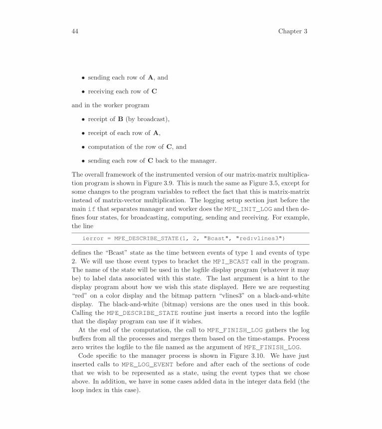
44 Chapter 3
• sending each row of A, and
• receiving each row of C
and in the worker program
• receipt of B (by broadcast),
• receipt of each row of A,
• computation of the row of C, and
• sending each row of C back to the manager.
The overall framework of the instrumented version of our matrix-matrix multiplica-
tion program is shown in Figure 3.9. This is much the same as Figure 3.5, except for
some changes to the program variables to reflect the fact that this is matrix-matrix
instead of matrix-vector multiplication. The logging setup section just before the
main if that separates manager and worker does the MPE_INIT_LOG and then de-
fines four states, for broadcasting, computing, sending and receiving. For example,
the line
ierror = MPE_DESCRIBE_STATE(1, 2, "Bcast", "red:vlines3")
defines the “Bcast” state as the time between events of type 1 and events of type
2. We will use those event types to bracket the MPI_BCAST call in the program.
The name of the state will be used in the logfile display program (whatever it may
be) to label data associated with this state. The last argument is a hint to the
display program about how we wish this state displayed. Here we are requesting
“red” on a color display and the bitmap pattern “vlines3” on a black-and-white
display. The black-and-white (bitmap) versions are the ones used in this book.
Calling the MPE_DESCRIBE_STATE routine just inserts a record into the logfile
that the display program can use if it wishes.
At the end of the computation, the call to MPE_FINISH_LOG gathers the log
buffers from all the processes and merges them based on the time-stamps. Process
zero writes the logfile to the file named as the argument of MPE_FINISH_LOG.Code specific to the manager process is shown in Figure 3.10. We have just
inserted calls to MPE_LOG_EVENT before and after each of the sections of code
that we wish to be represented as a state, using the event types that we chose
above. In addition, we have in some cases added data in the integer data field (the
loop index in this case).

Using MPI in Simple Programs 45
! matmat.f - matrix - matrix multiply,! simple self-scheduling version
program mainuse mpiinteger MAX_AROWS, MAX_ACOLS, MAX_BCOLSparameter (MAX_AROWS = 20, MAX_ACOLS = 1000, MAX_BCOLS = 20)double precision a(MAX_AROWS,MAX_ACOLS), b(MAX_ACOLS,MAX_BCOLS)double precision c(MAX_AROWS,MAX_BCOLS)double precision buffer(MAX_ACOLS), ans(MAX_BCOLS)double precision starttime, stoptimeinteger myid, master, numprocs, ierr, status(MPI_STATUS_SIZE)integer i, j, numsent, senderinteger anstype, row, arows, acols, brows, bcols, crows, ccolscall MPI_INIT(ierr)call MPI_COMM_RANK(MPI_COMM_WORLD, myid, ierr)call MPI_COMM_SIZE(MPI_COMM_WORLD, numprocs, ierr)arows = 10acols = 20brows = 20bcols = 10crows = arowsccols = bcolsmaster = 0ierr = MPE_INIT_LOG()if (myid .eq. 0) then
ierr = MPE_DESCRIBE_STATE(1, 2, "Bcast", "red:vlines3")ierr = MPE_DESCRIBE_STATE(3, 4, "Compute","blue:gray3")ierr = MPE_DESCRIBE_STATE(5, 6, "Send", "green:light_gray")ierr = MPE_DESCRIBE_STATE(7, 8, "Recv", "yellow:gray")
endifif (myid .eq. 0) then
! master initializes and then dispatches ...else
! slaves receive b, then compute rows of c ...endifierr = MPE_FINISH_LOG("pmatmat.log")call MPI_FINALIZE(ierr)end
Figure 3.9: Matrix-matrix multiplication with logging: common part
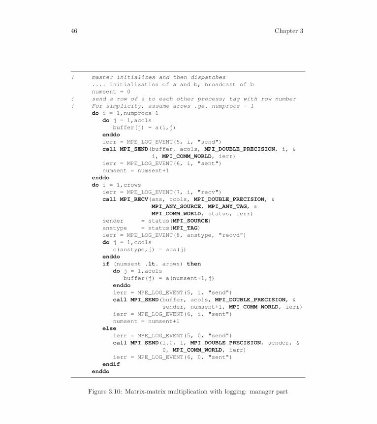
46 Chapter 3
! master initializes and then dispatches.... initialization of a and b, broadcast of bnumsent = 0
! send a row of a to each other process; tag with row number! For simplicity, assume arows .ge. numprocs - 1
do i = 1,numprocs-1do j = 1,acols
buffer(j) = a(i,j)enddoierr = MPE_LOG_EVENT(5, i, "send")call MPI_SEND(buffer, acols, MPI_DOUBLE_PRECISION, i, &
i, MPI_COMM_WORLD, ierr)ierr = MPE_LOG_EVENT(6, i, "sent")numsent = numsent+1
enddodo i = 1,crows
ierr = MPE_LOG_EVENT(7, i, "recv")call MPI_RECV(ans, ccols, MPI_DOUBLE_PRECISION, &
MPI_ANY_SOURCE, MPI_ANY_TAG, &MPI_COMM_WORLD, status, ierr)
sender = status(MPI_SOURCE)anstype = status(MPI_TAG)ierr = MPE_LOG_EVENT(8, anstype, "recvd")do j = 1,ccols
c(anstype,j) = ans(j)enddoif (numsent .lt. arows) then
do j = 1,acolsbuffer(j) = a(numsent+1,j)
enddoierr = MPE_LOG_EVENT(5, i, "send")call MPI_SEND(buffer, acols, MPI_DOUBLE_PRECISION, &
sender, numsent+1, MPI_COMM_WORLD, ierr)ierr = MPE_LOG_EVENT(6, i, "sent")numsent = numsent+1
elseierr = MPE_LOG_EVENT(5, 0, "send")call MPI_SEND(1.0, 1, MPI_DOUBLE_PRECISION, sender, &
0, MPI_COMM_WORLD, ierr)ierr = MPE_LOG_EVENT(6, 0, "sent")
endifenddo
Figure 3.10: Matrix-matrix multiplication with logging: manager part
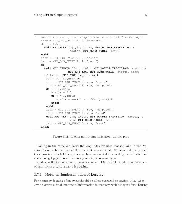
Using MPI in Simple Programs 47
! slaves receive b, then compute rows of c until done messageierr = MPE_LOG_EVENT(1, 0, "bstart")do i = 1,bcols
call MPI_BCAST(b(1,i), brows, MPI_DOUBLE_PRECISION, &master, MPI_COMM_WORLD, ierr)
enddoierr = MPE_LOG_EVENT(2, 0, "bend")ierr = MPE_LOG_EVENT(7, i, "recv")do
call MPI_RECV(buffer, acols, MPI_DOUBLE_PRECISION, master, &MPI_ANY_TAG, MPI_COMM_WORLD, status, ierr)
if (status(MPI_TAG) .eq. 0) exitrow = status(MPI_TAG)ierr = MPE_LOG_EVENT(8, row, "recvd")ierr = MPE_LOG_EVENT(3, row, "compute")do i = 1,bcols
ans(i) = 0.0do j = 1,acols
ans(i) = ans(i) + buffer(j)*b(j,i)enddo
enddoierr = MPE_LOG_EVENT(4, row, "computed")ierr = MPE_LOG_EVENT(5, row, "send")call MPI_SEND(ans, bcols, MPI_DOUBLE_PRECISION, master, &
row, MPI_COMM_WORLD, ierr)ierr = MPE_LOG_EVENT(6, row, "sent")
enddo
Figure 3.11: Matrix-matrix multiplication: worker part
We log in the “receive” event the loop index we have reached, and in the “re-
ceived” event the number of the row that was received. We have not really used
the character data field here, since we have not varied it according to the individual
event being logged; here it is merely echoing the event type.
Code specific to the worker process is shown in Figure 3.11. Again, the placement
of calls to MPE_LOG_EVENT is routine.
3.7.6 Notes on Implementation of Logging
For accuracy, logging of an event should be a low-overhead operation. MPE_Log_-event stores a small amount of information in memory, which is quite fast. During

48 Chapter 3
����� ����� ����� ����� ����� ���� ����
�� �� ������� ���� ����
�
�
�
�
�
Figure 3.12: Upshot output
MPE_Finish_log, these buffers are merged in parallel, and the final buffer, sorted
by time-stamp, is written out by process 0.
One subtle aspect of collecting logs with time-stamps is the necessity of relying
on local clocks. On some parallel computers there are synchronized clocks, but on
others the clocks are only approximately synchronized. On workstation networks,
the situation is much worse, and clocks even drift with respect to each other as
well.
To compensate for this situation, the time-stamps are postprocessed with respect
to synchronizations at MPE_Init_log and MPE_Finish_log. Postprocessing,
which includes aligning and stretching the time axes of each process so that the
MPE_Init_log and MPE_Finish_log take place at the same time, is done as
part of MPE_Finish_log. MPI itself is used to combine the logs, and the com-
bining process is done in parallel, with the logfile itself written out by the process
with rank 0 in MPI_COMM_WORLD.
3.7.7 Graphical Display of Logfiles
After an MPI program instrumented with the MPE logging routines has completed,
the directory where it executed contains a file of events sorted by time, with time
adjusted to correct for offset and drift. We can write many programs to extract
useful data from this file. One that we describe here and use from time to time
in the rest of this book is the graphical display program upshot. A sample of
upshot output is shown in Figure 3.12, which displays a portion of the logfile
collected while running the matrix-matrix multiplication program on six Suns on
an Ethernet. One can tell which one was the Sparc-10; the others were Sparc-2’s.
Upshot displays parallel time lines, with states indicated by colored bars on color
displays and patterns of dots or lines on monochrome displays (like the page of this

Using MPI in Simple Programs 49
book). Time-stamp values, adjusted to start at 0, are shown along the bottom of
the frame. A particular view is shown in Figure 3.12.
Of course, the information in logfiles can be displayed in simple summary form
as well, without graphics. The logfile is easy to parse with other tools as well.
For example, we can add up the time intervals recorded for each state, getting
something like the following.
State: Time:Bcast 0.146799Compute 0.044800Send 0.030711Recv 0.098852-----------------Total: 0.321162
Such summary information is a crude form of profiling; it tells us where the
program is spending its time. Note that since the events and states may be described
by the programmer and are not tied to the message-passing library, the MPE library
can be useful in studying aspects of an algorithm that have nothing to do with
interprocess communication.
3.8 Using Communicators
Up to this point, all our examples have used MPI_COMM_WORLD as an argument to
nearly every MPI call. What is it for, if it is always the same? In this section we
describe communicators, which are perhaps the most pervasive and distinguishing
feature of the MPI library specification. While a more comprehensive discussion
of the purpose and use of communicators occurs in Chapter 6, we give here an
extremely simple example that illustrates some of the MPI functions dealing with
groups and communicators.
The example will illustrate the Monte Carlo method of integration. We will use
it to find (again) the value of π. This will not be a particularly good way to find
the value of π, but it will provide us with a simple example. To make it more
interesting, we will introduce here some of the MPE real-time graphics operations,
so that we can watch our program in action.
In Figure 3.13, if the radius of the circle is 1, then the area is π and the area
of the square around it is 4. Therefore the ratio r of the area of the circle to that
of the square is π/4. We will compute the ratio r by generating random points
(x, y) in the square and counting how many of them turn out to be in the circle (by
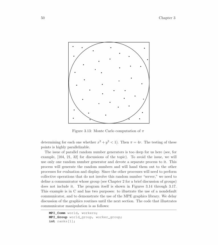
50 Chapter 3
Figure 3.13: Monte Carlo computation of π
determining for each one whether x2 + y2 < 1). Then π = 4r. The testing of these
points is highly parallelizable.
The issue of parallel random number generators is too deep for us here (see, for
example, [104, 21, 32] for discussions of the topic). To avoid the issue, we will
use only one random number generator and devote a separate process to it. This
process will generate the random numbers and will hand them out to the other
processes for evaluation and display. Since the other processes will need to perform
collective operations that do not involve this random number “server,” we need to
define a communicator whose group (see Chapter 2 for a brief discussion of groups)
does not include it. The program itself is shown in Figures 3.14 through 3.17.
This example is in C and has two purposes: to illustrate the use of a nondefault
communicator, and to demonstrate the use of the MPE graphics library. We delay
discussion of the graphics routines until the next section. The code that illustrates
communicator manipulation is as follows:
MPI_Comm world, workers;MPI_Group world_group, worker_group;int ranks[1];

Using MPI in Simple Programs 51
MPI_Init(&argc,&argv);world = MPI_COMM_WORLD;MPI_Comm_size(world, &numprocs);MPI_Comm_rank(world, &myid);server = numprocs-1; /* last process is server */
MPI_Comm_group(world, &world_group);ranks[0] = server;MPI_Group_excl(world_group, 1, ranks, &worker_group);MPI_Comm_create(world, worker_group, &workers);MPI_Group_free(&worker_group);MPI_Group_free(&world_group);
The new feature here is that we have two communicators, world and workers.The communicator workers will contain all the processes except the random num-
ber server. This code illustrates how to build a communicator that has all the
processes except the server process in it. To do this, we deal explicitly with the
group of processes associated with the default communicator MPI_COMM_WORLD.Let us go through this code line by line.
Two communicators, world and workers, are declared, along with two groups
of processes, world_group and worker_group. In C, an MPI group is described
by a MPI_Group type. After the required call to MPI_Init, we assign MPI_-COMM_WORLD to world. We find out how many processes there are with the call
to MPI_Comm_size, and we assign to server the rank of the last process in the
original group. The next few lines of code build the communicator that has as
its group all of the processes except the random number server. First we extract
from the MPI_COMM_WORLD communicator its group, which contains all processes.
This is done with a call to MPI_Comm_Group. It returns in world_group the
group of all processes. Next we build a new group. Groups can be manipulated in
many ways (see Chapter 7), but here the simplest approach is to use MPI_Group_-excl, which takes a given group and forms a new group by excluding certain of the
original group’s members. The members to be excluded are specified with an array
of ranks; here we exclude a single process. Then the call to MPI_Group_exclreturns in worker_group the new group, containing all the processes except the
random number server. We create the new communicator from MPI_COMM_WORLDby calling MPI_Comm_create with the old communicator and the new group,
getting back the new communicator in workers. This is the communicator we
will use for collective operations that do not involve the random number server. At
the end of the program, we release this communicator with a call to MPI_Comm_-
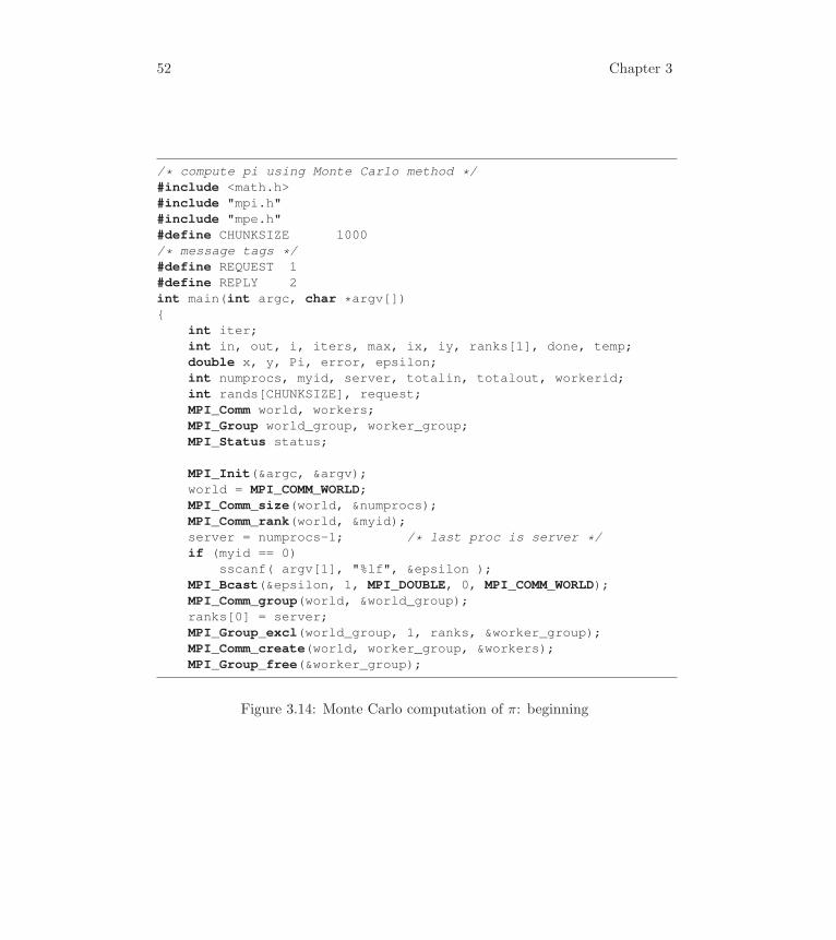
52 Chapter 3
/* compute pi using Monte Carlo method */#include <math.h>#include "mpi.h"#include "mpe.h"#define CHUNKSIZE 1000/* message tags */#define REQUEST 1#define REPLY 2int main(int argc, char *argv[]){
int iter;int in, out, i, iters, max, ix, iy, ranks[1], done, temp;double x, y, Pi, error, epsilon;int numprocs, myid, server, totalin, totalout, workerid;int rands[CHUNKSIZE], request;MPI_Comm world, workers;MPI_Group world_group, worker_group;MPI_Status status;
MPI_Init(&argc, &argv);world = MPI_COMM_WORLD;MPI_Comm_size(world, &numprocs);MPI_Comm_rank(world, &myid);server = numprocs-1; /* last proc is server */if (myid == 0)
sscanf( argv[1], "%lf", &epsilon );MPI_Bcast(&epsilon, 1, MPI_DOUBLE, 0, MPI_COMM_WORLD);MPI_Comm_group(world, &world_group);ranks[0] = server;MPI_Group_excl(world_group, 1, ranks, &worker_group);MPI_Comm_create(world, worker_group, &workers);MPI_Group_free(&worker_group);
Figure 3.14: Monte Carlo computation of π: beginning

Using MPI in Simple Programs 53
if (myid == server) { /* I am the rand server */do {
MPI_Recv(&request, 1, MPI_INT, MPI_ANY_SOURCE, REQUEST,world, &status);
if (request) {for (i = 0; i < CHUNKSIZE; ) {
rands[i] = random();if (rands[i] <= INT_MAX) i++;
}MPI_Send(rands, CHUNKSIZE, MPI_INT,
status.MPI_SOURCE, REPLY, world);}
}while(request > 0);
}
Figure 3.15: Monte Carlo computation of π: server
free. Finally, since we needed only the group worker_group in order to create
the workers communicator, we may now release it by calling MPI_Group_free.The code that “tidies up” by freeing the group and communicator that we created
during the run merits further discussion, because it illustrates an important point:
communicators contain internal references to groups. When we extract the group
explicitly, by a call to MPI_Comm_group, we create another reference to the group.
Later on, when we call MPI_Group_free with this reference, we are freeing the
reference, which becomes invalid, but we are not destroying the group itself, since
there is another reference inside the communicator. For this reason, we may actually
call
MPI_Group_free(&worker_group);
and
MPI_Comm_free(&workers);
in either order; the group does not cease to exist until both references to the group
have been freed. As an aid to safe programming, MPI sets the arguments to a free
call to a special null object; this makes it easier to detect the inadvertent use of an
(now) invalid object. These null objects have names (so that one can test for them);
they are MPI_GROUP_NULL and MPI_COMM_NULL. Others will be introduced as
they are needed.
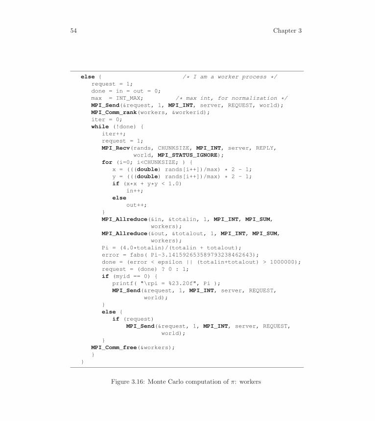
54 Chapter 3
else { /* I am a worker process */request = 1;done = in = out = 0;max = INT_MAX; /* max int, for normalization */MPI_Send(&request, 1, MPI_INT, server, REQUEST, world);MPI_Comm_rank(workers, &workerid);iter = 0;while (!done) {
iter++;request = 1;MPI_Recv(rands, CHUNKSIZE, MPI_INT, server, REPLY,
world, MPI_STATUS_IGNORE);for (i=0; i<CHUNKSIZE; ) {
x = (((double) rands[i++])/max) * 2 - 1;y = (((double) rands[i++])/max) * 2 - 1;if (x*x + y*y < 1.0)
in++;else
out++;}MPI_Allreduce(&in, &totalin, 1, MPI_INT, MPI_SUM,
workers);MPI_Allreduce(&out, &totalout, 1, MPI_INT, MPI_SUM,
workers);Pi = (4.0*totalin)/(totalin + totalout);error = fabs( Pi-3.141592653589793238462643);done = (error < epsilon || (totalin+totalout) > 1000000);request = (done) ? 0 : 1;if (myid == 0) {
printf( "\rpi = %23.20f", Pi );MPI_Send(&request, 1, MPI_INT, server, REQUEST,
world);}else {
if (request)MPI_Send(&request, 1, MPI_INT, server, REQUEST,
world);}
MPI_Comm_free(&workers);}
}
Figure 3.16: Monte Carlo computation of π: workers

Using MPI in Simple Programs 55
if (myid == server) { /* I am the rand server */...
} else { /* I am a worker process */...
}if (myid == 0) {
printf( "\npoints: %d\nin: %d, out: %d, <ret> to exit\n",totalin+totalout, totalin, totalout );
getchar();}MPI_Finalize();
}
Figure 3.17: Monte Carlo computation of π: ending
The code in Figure 3.16 also introduces a new feature. We’ve talked about MPI_-Recv and the status parameter; for Fortran programs, this is an output parame-
ter of type integer status(MPI_STATUS_SIZE). But what if you don’t want
any of the information that the status parameter provides? In that case, in either
C or Fortran, you can pass the special value MPI_STATUS_IGNORE. This does justwhat it says—ignore the status parameter.
The other new MPI library call introduced in this example is MPI_Allreduce.This differs from the MPI_Reduce that we have seen before in that the result of
the reduction operation is available in all processes, not just in the one specified as
root. Depending on implementation, MPI_Allreduce may be more efficient than
the equivalent MPI_Reduce followed by an MPI_Bcast. Here we use it to test
whether it is time to stop. We have provided an error value on the command line,
and each process compares the current value of π with the precalculated value we
have put into the program.
The specific bindings for the functions used in the Monte Carlo example are
shown in Tables 3.7 and 3.8.
3.9 Another Way of Forming New Communicators
The preceding example was useful in introducing the notions of MPI groups and
communicators. However, there is a slightly easier way of creating new communi-
cators containing a subset of the processes in an existing communicator.

56 Chapter 3
int MPI Allreduce(const void *sendbuf, void *recvbuf, int count,MPI Datatype datatype, MPI Op op, MPI Comm comm)
int MPI Comm group(MPI Comm comm, MPI Group *group)
int MPI Group excl(MPI Group group, int n, const int ranks[],
MPI Group *newgroup)
int MPI Group free(MPI Group *group)
int MPI Comm create(MPI Comm comm, MPI Group group,
MPI Comm *newcomm)
int MPI Comm free(MPI Comm *comm)
Table 3.7: C bindings for new routines needed by Monte Carlo example
MPI ALLREDUCE(sendbuf, recvbuf, count, datatype, op, comm, ierror)
<type> sendbuf(*), recvbuf(*)integer count, datatype, op, comm, ierror
MPI COMM GROUP(comm, group, ierror)integer comm, group, ierror
MPI GROUP EXCL(group, n, ranks, newgroup, ierror)
integer group, n, ranks(*), newgroup, ierror
MPI GROUP FREE(group, ierror)integer group, ierror
MPI COMM CREATE(comm, group, newcomm, ierror)integer comm, group, newcomm, ierror
MPI COMM FREE(comm, ierror)integer comm, ierror
Table 3.8: Fortran bindings for new routines needed by Monte Carlo example

Using MPI in Simple Programs 57
int MPI Comm split(MPI Comm oldcomm, int color, int key,
MPI Comm *newcomm)
Table 3.9: C binding for splitting communicators
MPI COMM SPLIT(oldcomm, color, key, newcomm, ierror)integer oldcomm, color, key, newcomm, ierror
Table 3.10: Fortran binding for splitting communicators
MPI_Comm_split is a collective operation taking as input a communicator and
two integers, called the color and the key, returning a new communicator. All
the processes that pass in the same value of color will be placed in the same com-
municator, and that communicator will be the one returned to them. The bindings
for MPI_Comm_split is shown in Table 3.9 and 3.10.
The key argument is used to assign ranks to the processes in the new commu-
nicator. If all processes passing the same value of color also pass the same value
of key, then they are given ranks in the new communicator that are in the same
order as their ranks in the old communicator. If they pass in different values for
key, then these values are used to determine their order in the new communicator.
Note that MPI_Comm_split creates several new communicators (one for each
color value) but that each process is given access only to one of the new communi-
cators, the one whose group the process belongs to.
The alternative way of creating new communicators out of MPI_COMM_WORLDsimplifies our program substantially. Instead of manipulating the groups of the
communicators directly, we create the communicator for the workers by having all
of them pass to MPI_Comm_split the same color value, but one that is different
from that passed in by the server. All the code involving group extraction and the
call to MPI_Comm_create is replaced by
color = (myid == server);MPI_Comm_split(world, color, 0, &workers);
3.10 A Handy Graphics Library for Parallel Programs
A second reason for including this Monte Carlo example is that it allows us to in-
troduce in its simplest possible form the MPE graphics library. In many programs,
parallel or not, it would be convenient to provide some simple graphics output.
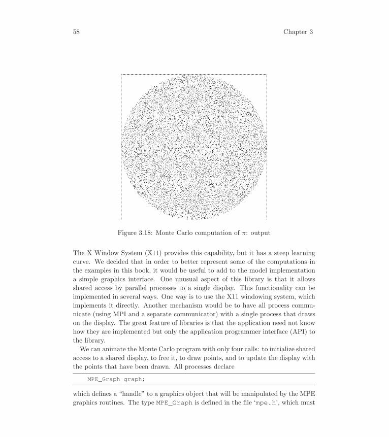
58 Chapter 3
Figure 3.18: Monte Carlo computation of π: output
The X Window System (X11) provides this capability, but it has a steep learning
curve. We decided that in order to better represent some of the computations in
the examples in this book, it would be useful to add to the model implementation
a simple graphics interface. One unusual aspect of this library is that it allows
shared access by parallel processes to a single display. This functionality can be
implemented in several ways. One way is to use the X11 windowing system, which
implements it directly. Another mechanism would be to have all process commu-
nicate (using MPI and a separate communicator) with a single process that draws
on the display. The great feature of libraries is that the application need not know
how they are implemented but only the application programmer interface (API) to
the library.
We can animate the Monte Carlo program with only four calls: to initialize shared
access to a shared display, to free it, to draw points, and to update the display with
the points that have been drawn. All processes declare
MPE_Graph graph;
which defines a “handle” to a graphics object that will be manipulated by the MPE
graphics routines. The type MPE_Graph is defined in the file ‘mpe.h’, which must

Using MPI in Simple Programs 59
be included. At the beginning of the program, all processes might do
MPE_Open_graphics(&graph, MPI_COMM_WORLD, (char *)0, -1, -1,WINDOW_SIZE, WINDOW_SIZE, MPE_GRAPH_INDEPENDENT);
which initializes this handle. The arguments in this case specify that the communi-
cator MPI_COMM_WORLD will be used for communication for this graphics object,
that the default display from the user’s environment should be used as the X dis-
play ((char *)0 as third argument instead of a display name), and that the user
will be asked to place the window that is created. One could specify a location
(x,y) by using non-negative integers instead of (-1, -1). The rest of the arguments
specify that the window will be square with side WINDOW_SIZE and that graphics
operations will not be collective. For details, see Appendix A.
At the end of the program, each process does
MPE_Close_graphics(&graph);
to terminate access to the display. The only drawing command in this program is
used to draw single points on the display. We will draw the points that lie within
the circle of radius 1. Therefore, as more points are generated, we expect to see a
rounder and rounder circle emerge. We can see this happening in Figure 3.18. The
subroutine call
MPE_Draw_point(graph,(int)(WINDOW_SIZE/2 + x*WINDOW_SIZE/2),(int)(WINDOW_SIZE/2 - y*WINDOW_SIZE/2),MPE_BLACK);
draws a point at the two coordinates given by its second and third arguments, in
the color given by its last argument (of type MPE_Color). The line
MPE_Update(graph);
causes all of the drawing actions that may have been buffered up to this point to
be flushed to the display. We can cut down on traffic to the X server by calling
this only after a large number of calls to MPE_Draw_point. In our program (not
shown in this book) MPE_Update is called after each process has finished with one
batch of points.

60 Chapter 3
3.11 Common Errors and Misunderstandings
Experience with helping people learn MPI has helped us identify a set of mistakes
that users often make. In this section we call your attention to some of them in the
hope that we can help you avoid them right from the beginning.
Forgetting ierr in Fortran. Perhaps the most common error made in MPI
programs written in Fortran is to forget the last argument, where the error code is
returned. Some Fortran compilers will catch this at compile time, but others will
not, leading to hard-to-find errors.
Misdeclaring status in Fortran. When an MPI_Recv returns, certain infor-
mation has been stored in the status argument. Status is an array of integers
(of size MPI_STATUS_SIZE), not a single integer. Many compilers will not com-
plain about this, but running the program will definitely lead to an unexpected
memory overwrite and mysterious behavior.
Misdeclaring string variables in Fortran. In Fortran, strings are not the same
as arrays of characters. Although this is not really an MPI issue, MPI does use
string variables, and so this error sometimes happens when someone uses MPI for
the first time. A ten-character string a in Fortran should be declared as something
like
character*10 a
and definitely not
character a(10)
The latter is an array of characters, not a single character string variable.
Expecting argc and argv to be passed to all processes. The arguments to
MPI_Init in C are &argc and &argv. This feature allows the MPI implementa-
tion to fill these in on all processes, but the MPI standard does not require it. Some
implementations propagate argc and argv to all processes; some don’t. The same
is true for the environment (variables whose values are accessible by getenv); some
implementations may start all processes with the environment in existence when
mpirun or mpiexec is run, but others may not. A portable program will not rely
on this feature. Remember that MPI does not assume it is running under Unix,
and some MPI implementations run on Windows or in specialized (e.g., real-time)
Using MPI in Simple Programs 61
environments. MPI-3 provides a way to access some of this information with a
predefined MPI_Info object, MPI_INFO_ENV. MPI_Info is described in Using
Advanced MPI [55].
Doing things before MPI_Init or after MPI_Finalize. The MPI standard
says little about the situation before MPI_Init or after MPI_Finalize, not evenhow many processes are running. Doing anything whatsoever in your program
during either of these periods may yield unexpected and implementation-dependent
results. For example, argc and argv may not make any sense until after MPI_-Init has processed them, and so an MPI application should not access them until
then. One exception is the behavior after MPI_Finalize returns. The MPI
standard guarantees that at least the process with rank zero in MPI_COMM_WORLDwill continue executing after MPI_Finalize returns. This permits an application
to perform any non-MPI cleanup and, in a POSIX environment, provide an exit
code for the program. If you use this feature, make sure to test that the process is
the one with rank zero in MPI_COMM_WORLD—after MPI_Finalize, it’s possiblethat all MPI processes are still running.
Matching MPI_Bcast with MPI_Recv. It is easy to think that MPI_Bcast is
a “multiple send” operation, and that the recipients of the broadcast message should
receive it with MPI_Recv. On the contrary, MPI_Bcast is a collective operation
that must be called on all processes in the group of the specified communicator.
It functions as a multisend on the specified root process and as a receive on the
others. The reason is that it allows for optimal performance. An MPI_Recv does
not have to check whether the message it has just received is part of a broadcast
and hence may have to be forwarded to other processes.
Assuming your MPI implementation is thread-safe. We discussed multi-
threading in Chapter 1. MPI was designed so that it could be implemented in a
thread-safe manner (multiple threads could call MPI routines at the same time) but
the standard does not require it of implementations. If you use multithreading in
your program (or even if your compiler generates multithreaded code for you) and
your MPI implementation is not thread-safe, you may get unpredictable results.
See Using Advanced MPI [55] for a discussion of the MPI-2 features that make
MPI’s interaction with threads more explicit.

62 Chapter 3
3.12 Summary of a Simple Subset of MPI
In this chapter we have introduced basic MPI routines through simple example
programs. In particular, we have defined the six functions that make up the minimal
MPI subset that we discussed in Chapter 2. We have added to those the two most
common collective operations and the basic timing routine, and we have shown how
to work with groups and communicators. We have also introduced a few useful
tools: MPE logging, MPE graphics, and upshot, as representative of a class of
widely available performance analysis tools. We will continue to use these tools as
we look at more example programs in the chapters to come. Additionally, we have
summarized a few of the common problems that MPI beginners sometimes make.
In some ways we have already provided enough of the MPI library to write serious
applications. In other ways we have barely scratched the surface. MPI offers much
more, as we will see in the upcoming chapters.
The following section is the first of our “Application” sections. These appear at
the end of several chapters. You might want to skip these if you are reading the book
sequentially, since in many cases they require considerable study and knowledge of
the particular field in order to understand fully. We include them to demonstrate
the range and complexity of scientific applications that have been enabled by MPI.
3.13 Application: Computational Fluid Dynamics
The following application illustrates the usefulness of user-defined virtual topologies
and collective communication over these virtual topologies, all within a computa-
tional fluid dynamics code. It illustrates the use of operations on communicators to
define topologies not provided directly by MPI. The use of MPI topology definition
routines will be explained in the next chapter. The computation of flow regimes
over complex configurations involves the numerical solution of a system of cou-
pled nonlinear partial differential equations known as the Navier-Stokes equations.
Researchers in the CFD lab at the Mississippi State University NSF Engineering
Research Center for Computational Field Simulation have developed an implicit,
finite-volume code (known as UNCLE) for solving the unsteady three-dimensional
incompressible Euler and Navier-Stokes equations using an artificial compressibility
approach [117, 116, 123]. The flow solver can be used in a variety of applications
ranging from maneuvering underwater vehicles to centrifugal compressors.
This code uses dynamic multiblock grids with relative motion in order to account
for complex moving geometries. Key elements of the solution method include high-
resolution, flux-based, upwind finite-volume approximations in time-varying trans-

Using MPI in Simple Programs 63
formed coordinates and a multiple-pass solution algorithm based on discretized
Newton relaxation [123]. The equations in the fully coupled unsteady form are
solved by using third-order spatial differencing for both steady and unsteady flows
and second-order time differencing for unsteady flows. Relaxation at each time step
is carried out by using a simple symmetric Gauss-Seidel sweeps. Turbulent flows
are simulated by using the Baldwin-Lomax turbulence model.
Large memory requirements and large run times severely restrict the size and
complexity of the problems that can be handled using the sequential version of
the code. Therefore, the need was identified for a scalable portable parallel ver-
sion that could take advantage of existing and emerging parallel platforms. The
message-passing interface required for the parallel implementation had to support
collective operations within user-defined groups as well as provide safe communica-
tion contexts for overlapping sets of collective operations (we will see an example
of overlapping communicators later in this section).
3.13.1 Parallel Formulation
The parallel formulation employs spatial decomposition of the overall grid into
subblocks that are assigned to separate processes [100]. To exploit coarse-grained
parallelism and message passing, the implicit subiteration algorithm was modified at
block interfaces to provide a block-decoupled algorithm. This decoupled algorithm
utilizes Gauss-Seidel relaxation sweeps within each process but is effectively explicit
at block boundaries, allowing parallel solution for all blocks. The solution at points
shared by neighboring processes is updated between each subiteration by means of
a message exchange.
The implementation of the Baldwin-Lomax turbulence model [25] introduces ad-
ditional complexity into the parallel implementation of the flow code. This mainly
affects the set-up phase of the solution process. The model requires the normal
derivative of the tangential velocity at all impermeable surfaces in order to calcu-
late the turbulent viscosity. This derivative is calculated in any block that includes
an impermeable surface. The values of the derivatives then are propagated along
the blocks that lie on any of the computational domain axes that begin with or ter-
minate in an impermeable boundary. The blocks that satisfy the above condition
are grouped together to share the derivative information. The turbulence model
further requires the calculation of the maxima and minima of quantities that are
distributed among the blocks of the above group.
The time-dependent equations in Cartesian coordinates are transformed into gen-
eral curvilinear coordinates while introducing the artificial compressibility terms

64 Chapter 3
Figure 3.19: Multiblock grid of physical domain for CFD problem
into the equations. The coordinate transformation essentially maps the arbitrary
shape of the region of interest to a computational domain that is a rectangular
parallelepiped. The solution procedure consists of two different phases. The first
involves setting up a linear system using appropriate flux formulation and lineariza-
tion techniques. The second phase is the solution of the linear system. The size
of the system is equal to four times the number of grid points in the domain and
could be of order 104–106 unknowns for realistic problems. However, the coefficient
matrix of the linear system is extremely sparse and is generally solved by using
iterative methods. From the parallel processing point of view, the set-up phase is
easily parallelizable, having local data dependencies and being confined to at most
13-point stencils for three-dimensional problems.
Mapping of the physical domain into a single rectangular parallelepiped is of-
ten not possible for complex geometries. This problem is resolved by resorting to
what are known as multiblock grids, where the physical domain is partitioned ap-
propriately before being mapped into a number of rectangular three-dimensional
domains that share common faces. This is shown in Figure 3.19. The linear system
in each block is solved by using symmetric Gauss-Seidel iterations with boundary
information being exchanged at the end of each forward and backward iteration
[116].
Key areas of the parallel implementation include (a) initialization of the flow
field, (b) duplication of stored data for points near block interfaces, (c) exchange of
data during subiterations, for points having duplicated storage, and (d) treatment
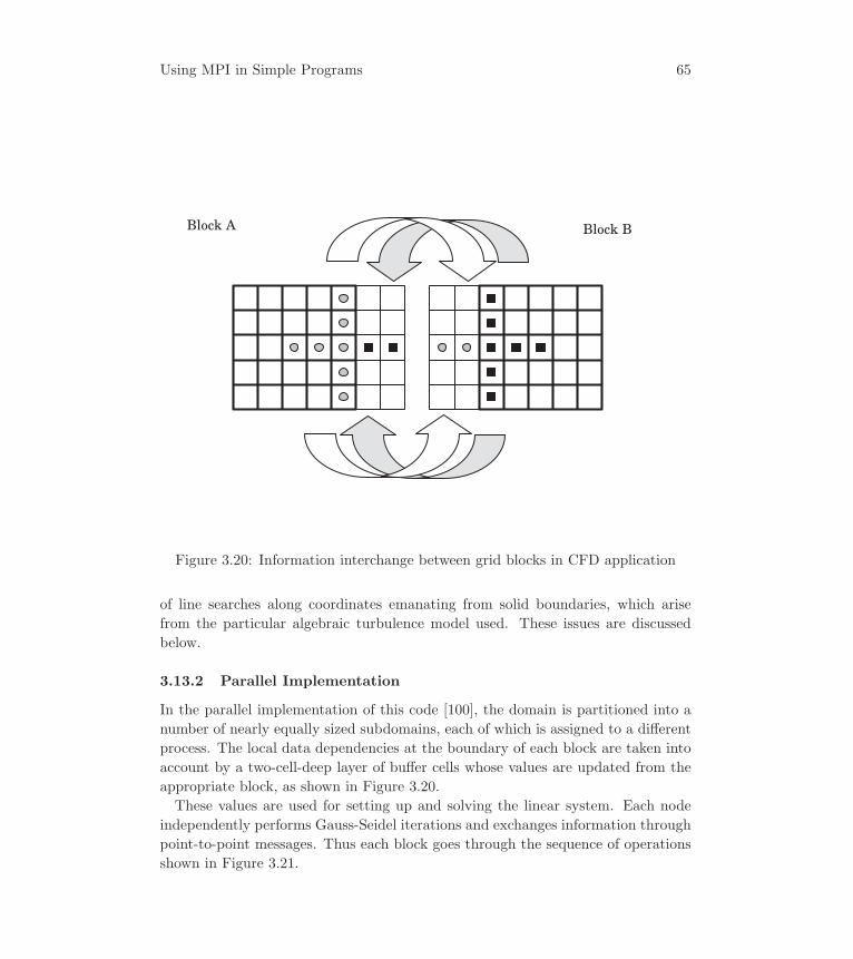
Using MPI in Simple Programs 65
Block A Block B
Figure 3.20: Information interchange between grid blocks in CFD application
of line searches along coordinates emanating from solid boundaries, which arise
from the particular algebraic turbulence model used. These issues are discussed
below.
3.13.2 Parallel Implementation
In the parallel implementation of this code [100], the domain is partitioned into a
number of nearly equally sized subdomains, each of which is assigned to a different
process. The local data dependencies at the boundary of each block are taken into
account by a two-cell-deep layer of buffer cells whose values are updated from the
appropriate block, as shown in Figure 3.20.
These values are used for setting up and solving the linear system. Each node
independently performs Gauss-Seidel iterations and exchanges information through
point-to-point messages. Thus each block goes through the sequence of operations
shown in Figure 3.21.
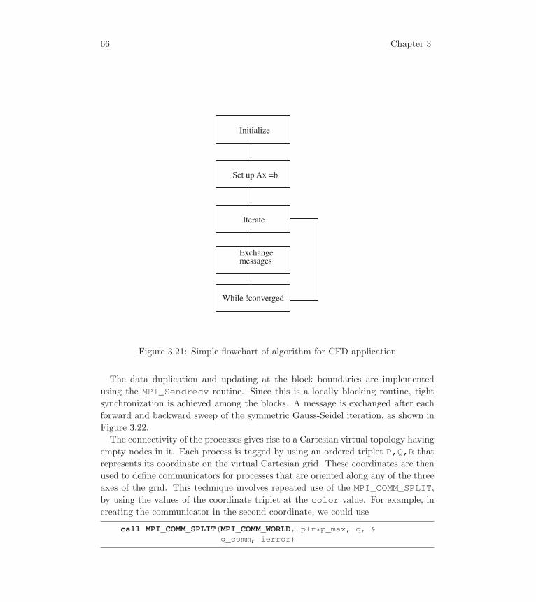
66 Chapter 3
Initialize
Set up Ax =b
Iterate
Exchangemessages
While !converged
Figure 3.21: Simple flowchart of algorithm for CFD application
The data duplication and updating at the block boundaries are implemented
using the MPI_Sendrecv routine. Since this is a locally blocking routine, tight
synchronization is achieved among the blocks. A message is exchanged after each
forward and backward sweep of the symmetric Gauss-Seidel iteration, as shown in
Figure 3.22.
The connectivity of the processes gives rise to a Cartesian virtual topology having
empty nodes in it. Each process is tagged by using an ordered triplet P,Q,R that
represents its coordinate on the virtual Cartesian grid. These coordinates are then
used to define communicators for processes that are oriented along any of the three
axes of the grid. This technique involves repeated use of the MPI_COMM_SPLIT,by using the values of the coordinate triplet at the color value. For example, in
creating the communicator in the second coordinate, we could use
call MPI_COMM_SPLIT(MPI_COMM_WORLD, p+r*p_max, q, &q_comm, ierror)

Using MPI in Simple Programs 67
ÇÇÇÇÇÇÇÇÇÇÇÇÇÇÇÇÇÇÇÇÇÇÇÇÇÇÇÇ
ÇÇÇÇÇÇÇÇÇÇÇÇÇÇÇÇÇÇÇÇÇÇÇÇÇÇÇÇÇÇÇÇÇÇÇÇ
(0,2) (1,2) (2,2)
(1,1)
(1,0)
(2,3)
(2,1)
(2,0)
I
J
ÇÇÇÇÇÇÇÇÇÇÇÇÇÇ
Figure 3.22: Communication pattern for CFD application with turbulence model
The communicators that are defined in this way form the basis for all the collective
operations needed for implementing the turbulence model.
The details of the parallel turbulence model implementation are shown in Fig-
ure 3.22. The blocks with the shaded borders have impermeable boundaries and
therefore calculate the velocity derivatives. The values of the derivative are then
broadcast to the blocks through which the arrows pass. This is done using the
MPI_BCAST routine within an appropriately defined communicator. Thus each
arrow represents a separate process group and its associated communicator. A
global MPI_ALLREDUCE operation using the local minimum and maximum leaves
the global minimum and maximum with each process that participates. The pat-
tern here shows overlapping communicators, as promised above. For each process,
there are two communicators: one for the row that the process is in and one for the
column. The code for the broadcasts in this step looks very roughly like
68 Chapter 3
call MPI_BCAST(deriv, count, MPI_DOUBLE_PRECISION, row_root, &row_comm, ierror)
call MPI_BCAST(deriv, count, MPI_DOUBLE_PRECISION, col_root, &col_comm, ierror)
This application illustrates how MPI can simplify the coding of a complex appli-
cation. The key simplifications that result come from the use of virtual topologies
and collective communication with the virtual topologies. Although the researchers
chose to use their own virtual topologies in this case, the availability of communica-
tors and the ease of building subset communicators with MPI_COMM_SPLIT made
programming easy. This application would be extremely difficult on a system that
was strictly a point-to-point message-passing interface without contexts of message
passing.

4 Intermediate MPI
In the preceding chapter we considered a number of straightforward parallel algo-
rithms. We wrote parallel programs for these algorithms using straightforward MPI
subroutine calls, and we verified with timing and program visualization tools that
our programs behaved as we expected.
In this chapter we introduce several important issues that require more subtlety in
our analysis and more precision in our tools. The mathematical problem we address
here (the Poisson problem) is only a little more complicated than the problems of
the preceding chapter, but the parallel algorithm, particularly the communication
pattern, admits more options.
We introduce several new MPI routines. For example, since our mathematical
problem takes place on a finite-difference computational grid, we introduce the MPI
notion of virtual topology, which makes the allocation of processes to particular parts
of a grid convenient to manage. We also describe many of the variations on the
basic send and receive operations supported by MPI; indeed, the communication
patterns needed here by our parallel algorithm motivated some of the more esoteric
MPI features.
Our first goal in this chapter is thus to show how MPI enables efficient programs
to be written concisely. A secondary goal is to explain some of the issues that arise
in analyzing communication patterns in grid-based problems.
We approach both of these goals by examining a number of programs for the 2-D
and 3-D Poisson problem, a model partial differential equation. Because Fortran
provides a much more convenient syntax for manipulating multidimensional arrays
than does C, the bulk of the examples in this chapter are written in Fortran.
We also use the Poisson problem as a means to introduce the different mechanisms
by which an MPI program can send data from one process to another, particularly
with respect to both how data is buffered in the message passing system and how
nonblocking communications can be used. By examining the different approaches
in the context of a single application, we clarify the distinctions between these
approaches. We begin by presenting the mathematical problem and an approach to
solving it computationally. Then we describe MPI’s virtual topology feature, which
allows us to manage a grid of processes. As we progress, we introduce several new
MPI functions while considering various ways of organizing the communications.
To help in understanding the reasons for the different implementation choices, we
also make another brief foray into scalability analysis.
This chapter may also be viewed as a discussion of the sparse matrix-vector
product, because that is really the fundamental operation at work in these algo-
rithms. While we will not discuss it in this book, the message-passing operations

70 Chapter 4
discussed in this chapter are the same as are used in implementing a parallel sparse
matrix-vector product. The Jacobi method was chosen for its simplicity in the
computational part of the program, allowing us to present a complete application.
4.1 The Poisson Problem
The Poisson problem is a simple partial differential equation (PDE) that is at the
core of many applications. More elaborate problems and algorithms often have the
same communication structure that we will use here to solve this problem. Thus,
by studying how MPI can be used here, we are providing fundamentals on how
communication patterns appear in more complex PDE problems. At the same
time, we can demonstrate a wide variety of message-passing techniques and how
MPI may be used to express them.
We emphasize that while the Poisson problem is a useful example for describing
the features of MPI that can be used in solving partial differential equations and
other problems that involve decomposition across many processes, the numerical
techniques in this section are not the last word in solving PDEs and give poor
performance relative to more recent and sophisticated methods. For information
on more sophisticated, freely available parallel solvers for PDEs that use MPI, see
[24]. For more details about the mathematical terminology used in this chapter,
consult [81], among other sources.
The Poisson problem is expressed by the following equations:
∇2u = f(x, y) in the interior (4.1)
u(x, y) = g(x, y) on the boundary (4.2)
To simplify the discussion, we use the unit square as the domain.
To find an approximate solution to this problem, we define a square mesh (also
called a grid) consisting of the points (xi, yj), given by
xi =i
n+ 1, i = 0, . . . , n+ 1,
yj =j
n+ 1, j = 0, . . . , n+ 1,
where there are n+ 2 points along each edge of the mesh (see Figure 4.1). We will
find an approximation to u(x, y) only at the points (xi, yj). We use the shorthand
ui,j to refer to the approximation to u at (xi, yj). The value 1/(n + 1) is used
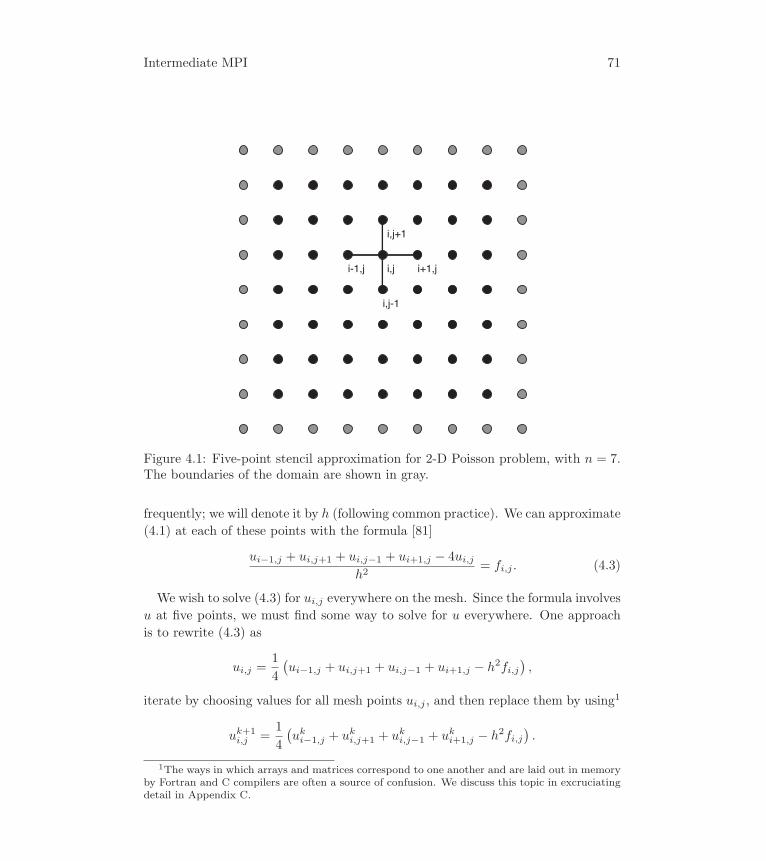
Intermediate MPI 71
i+1,j
i,j-1
i-1,j
i,j+1
i,j
Figure 4.1: Five-point stencil approximation for 2-D Poisson problem, with n = 7.The boundaries of the domain are shown in gray.
frequently; we will denote it by h (following common practice). We can approximate
(4.1) at each of these points with the formula [81]
ui−1,j + ui,j+1 + ui,j−1 + ui+1,j − 4ui,j
h2= fi,j . (4.3)
We wish to solve (4.3) for ui,j everywhere on the mesh. Since the formula involves
u at five points, we must find some way to solve for u everywhere. One approach
is to rewrite (4.3) as
ui,j =1
4
(ui−1,j + ui,j+1 + ui,j−1 + ui+1,j − h2fi,j
),
iterate by choosing values for all mesh points ui,j , and then replace them by using1
uk+1i,j =
1
4
(uki−1,j + uk
i,j+1 + uki,j−1 + uk
i+1,j − h2fi,j).
1The ways in which arrays and matrices correspond to one another and are laid out in memoryby Fortran and C compilers are often a source of confusion. We discuss this topic in excruciatingdetail in Appendix C.
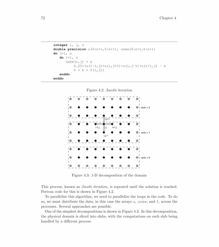
72 Chapter 4
integer i, j, ndouble precision u(0:n+1,0:n+1), unew(0:n+1,0:n+1)do j=1, n
do i=1, nunew(i,j) = &
0.25*(u(i-1,j)+u(i,j+1)+u(i,j-1)+u(i+1,j) - &h * h * f(i,j))
enddoenddo
Figure 4.2: Jacobi iteration
i+1,j
i,j-1
i-1,j
i,j+1
i,j
rank = 2
rank = 0
rank = 1
Figure 4.3: 1-D decomposition of the domain
This process, known as Jacobi iteration, is repeated until the solution is reached.
Fortran code for this is shown in Figure 4.2.
To parallelize this algorithm, we need to parallelize the loops in the code. To do
so, we must distribute the data, in this case the arrays u, unew, and f, across theprocesses. Several approaches are possible.
One of the simplest decompositions is shown in Figure 4.3. In this decomposition,
the physical domain is sliced into slabs, with the computations on each slab being
handled by a different process.
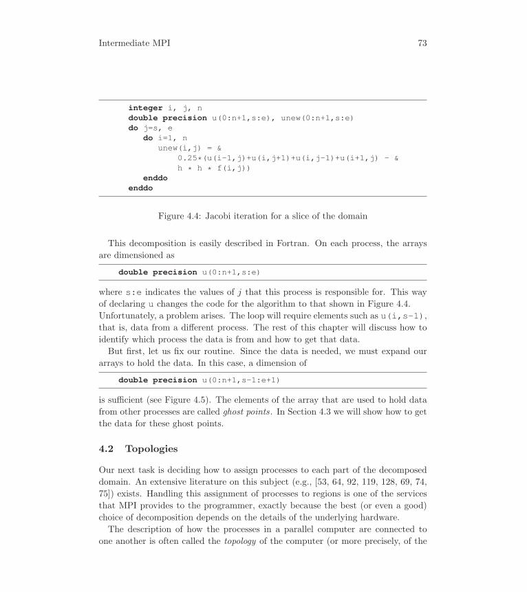
Intermediate MPI 73
integer i, j, ndouble precision u(0:n+1,s:e), unew(0:n+1,s:e)do j=s, e
do i=1, nunew(i,j) = &
0.25*(u(i-1,j)+u(i,j+1)+u(i,j-1)+u(i+1,j) - &h * h * f(i,j))
enddoenddo
Figure 4.4: Jacobi iteration for a slice of the domain
This decomposition is easily described in Fortran. On each process, the arrays
are dimensioned as
double precision u(0:n+1,s:e)
where s:e indicates the values of j that this process is responsible for. This way
of declaring u changes the code for the algorithm to that shown in Figure 4.4.
Unfortunately, a problem arises. The loop will require elements such as u(i,s-1),that is, data from a different process. The rest of this chapter will discuss how to
identify which process the data is from and how to get that data.
But first, let us fix our routine. Since the data is needed, we must expand our
arrays to hold the data. In this case, a dimension of
double precision u(0:n+1,s-1:e+1)
is sufficient (see Figure 4.5). The elements of the array that are used to hold data
from other processes are called ghost points. In Section 4.3 we will show how to get
the data for these ghost points.
4.2 Topologies
Our next task is deciding how to assign processes to each part of the decomposed
domain. An extensive literature on this subject (e.g., [53, 64, 92, 119, 128, 69, 74,
75]) exists. Handling this assignment of processes to regions is one of the services
that MPI provides to the programmer, exactly because the best (or even a good)
choice of decomposition depends on the details of the underlying hardware.
The description of how the processes in a parallel computer are connected to
one another is often called the topology of the computer (or more precisely, of the
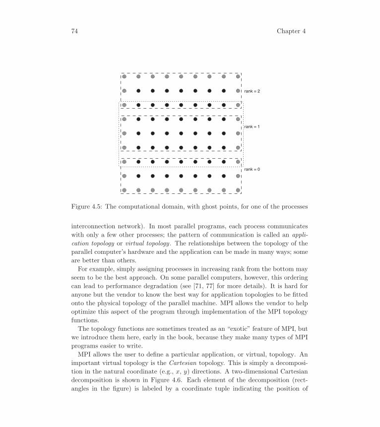
74 Chapter 4
rank = 1
rank = 2
rank = 0
Figure 4.5: The computational domain, with ghost points, for one of the processes
interconnection network). In most parallel programs, each process communicates
with only a few other processes; the pattern of communication is called an appli-
cation topology or virtual topology . The relationships between the topology of the
parallel computer’s hardware and the application can be made in many ways; some
are better than others.
For example, simply assigning processes in increasing rank from the bottom may
seem to be the best approach. On some parallel computers, however, this ordering
can lead to performance degradation (see [71, 77] for more details). It is hard for
anyone but the vendor to know the best way for application topologies to be fitted
onto the physical topology of the parallel machine. MPI allows the vendor to help
optimize this aspect of the program through implementation of the MPI topology
functions.
The topology functions are sometimes treated as an “exotic” feature of MPI, but
we introduce them here, early in the book, because they make many types of MPI
programs easier to write.
MPI allows the user to define a particular application, or virtual, topology. An
important virtual topology is the Cartesian topology. This is simply a decomposi-
tion in the natural coordinate (e.g., x, y) directions. A two-dimensional Cartesian
decomposition is shown in Figure 4.6. Each element of the decomposition (rect-
angles in the figure) is labeled by a coordinate tuple indicating the position of
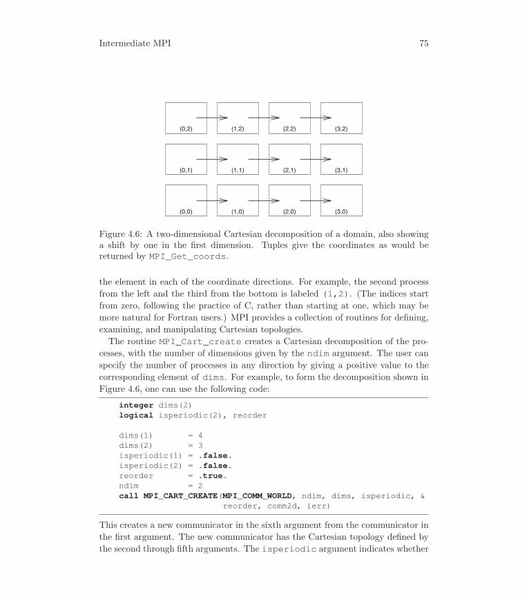
Intermediate MPI 75
(0,0) (1,0) (2,0) (3,0)
(0,1) (1,1) (2,1) (3,1)
(0,2) (1,2) (2,2) (3,2)
Figure 4.6: A two-dimensional Cartesian decomposition of a domain, also showinga shift by one in the first dimension. Tuples give the coordinates as would bereturned by MPI_Get_coords.
the element in each of the coordinate directions. For example, the second process
from the left and the third from the bottom is labeled (1,2). (The indices start
from zero, following the practice of C, rather than starting at one, which may be
more natural for Fortran users.) MPI provides a collection of routines for defining,
examining, and manipulating Cartesian topologies.
The routine MPI_Cart_create creates a Cartesian decomposition of the pro-
cesses, with the number of dimensions given by the ndim argument. The user can
specify the number of processes in any direction by giving a positive value to the
corresponding element of dims. For example, to form the decomposition shown in
Figure 4.6, one can use the following code:
integer dims(2)logical isperiodic(2), reorder
dims(1) = 4dims(2) = 3isperiodic(1) = .false.isperiodic(2) = .false.reorder = .true.ndim = 2call MPI_CART_CREATE(MPI_COMM_WORLD, ndim, dims, isperiodic, &
reorder, comm2d, ierr)
This creates a new communicator in the sixth argument from the communicator in
the first argument. The new communicator has the Cartesian topology defined by
the second through fifth arguments. The isperiodic argument indicates whether

76 Chapter 4
the processes at the “ends” are connected (for example, is the right neighbor of the
process at the right end the leftmost process in that row?). This is useful for
“periodic” domains. For example, in simulating the weather on the Earth within
the temperate latitudes using a three-dimensional grid with the dimensions referring
to east-west, north-south, and up-down, the first of these is periodic and the other
two are not.
Note that we have not specified which process is assigned to each of the ele-
ments of the decomposition. By setting the argument reorder to .true., wehave allowed MPI to find a good way to assign the process to the elements of the
decomposition.
In one dimension, we can simply use the rank in the new communicator, plus or
minus one, to find our neighbors (and not use MPI_Cart_create). Even here,
this may not be the best choice, because neighbors defined in this way may not be
neighbors in the actual hardware. In more than one dimension, however, it is more
difficult to determine the neighboring processes. The reorder argument, when
true, lets MPI know that it may reorder the processes for better performance.
Fortunately, MPI provides a simple way to find the neighbors of a Cartesian mesh.
The most direct way is to use the routine MPI_Cart_get. This routine returns
values of the dims and isperiodic argument used in MPI_Cart_create as
well as an array coords that contains the Cartesian coordinates of the calling
process. For example, the code
call MPI_CART_GET(comm2d, 2, dims, isperiodic, coords, ierr)print *, ’(’, coords(1), ’,’, coords(2), ’)’
will print the coordinates of the calling process in the communicator comm2d.Another way is to use MPI_Cart_coords; this routine, given a rank in a commu-
nicator, returns the coordinates of the process with that rank. For example, to get
the coordinates of the calling process, one can use
call MPI_COMM_RANK(comm2d, myrank, ierr)call MPI_CART_COORDS(comm2d, myrank, 2, coords, ierr)
However, another way exists that is more closely related to what we are trying to
accomplish. Each process needs to send and receive data from its neighbors. In the
1-D decomposition, these are the neighbors above and below. There are many ways
to do this transfer, but a simple one is illustrated in Figure 4.7. This represents a
copy of the top row from one process to the bottom ghost-point row of the process
above it, followed by a copy of the bottom row to the top ghost-point row of the
process below. If we look at the first of these operations, we see that each process
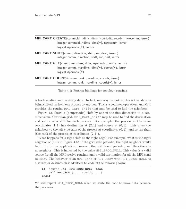
Intermediate MPI 77
MPI CART CREATE(commold, ndims, dims, isperiodic, reorder, newcomm, ierror)
integer commold, ndims, dims(*), newcomm, ierror
logical isperiodic(*),reorder
MPI CART SHIFT(comm, direction, shift, src, dest, ierror )integer comm, direction, shift, src, dest, ierror
MPI CART GET(comm, maxdims, dims, isperiodic, coords, ierror)
integer comm, maxdims, dims(*), coords(*), ierror
logical isperiodic(*)
MPI CART COORDS(comm, rank, maxdims, coords, ierror)
integer comm, rank, maxdims, coords(*), ierror
Table 4.1: Fortran bindings for topology routines
is both sending and receiving data. In fact, one way to look at this is that data is
being shifted up from one process to another. This is a common operation, and MPI
provides the routine MPI_Cart_shift that may be used to find the neighbors.
Figure 4.6 shows a (nonperiodic) shift by one in the first dimension in a two-
dimensional Cartesian grid. MPI_Cart_shiftmay be used to find the destination
and source of a shift for each process. For example, the process at Cartesian
coordinates (1, 1) has destination at (2, 1) and source at (0, 1). This gives the
neighbors to the left (the rank of the process at coordinates (0, 1)) and to the right
(the rank of the process at coordinates (2, 1)).
What happens for a right shift at the right edge? For example, what is the right
neighbor of (3, 0) in Figure 4.6? If the grid were periodic, the right neighbor would
be (0, 0). In our application, however, the grid is not periodic, and thus there is
no neighbor. This is indicated by the value MPI_PROC_NULL. This value is a valid
source for all the MPI receive routines and a valid destination for all the MPI send
routines. The behavior of an MPI_Send or MPI_Recv with MPI_PROC_NULL as
a source or destination is identical to code of the following form:
if (source .ne. MPI_PROC_NULL) thencall MPI_SEND(..., source, ...)
endif
We will exploit MPI_PROC_NULL when we write the code to move data between
the processes.

78 Chapter 4
(a) (b)
Figure 4.7: Two-step process to transfer data. Ghost point areas are shown indashed boxes; data to be moved is shaded. The mesh points are shown as blockcircles; the ghost points in the mesh are shown as unfilled circles.
int MPI Cart create(MPI Comm comm old, int ndims, const int dims[],
const int isperiodic[], int reorder, MPI Comm *new comm)
int MPI Cart shift(MPI Comm comm, int direction, int displ, int *src, int *dest)
int MPI Cart get(MPI Comm comm, int maxdims, int dims[], int isperiodic[],int coords[])
int MPI Cart coords(MPI Comm comm, int rank, int maxdims, int coords[])
Table 4.2: C bindings for topology routines
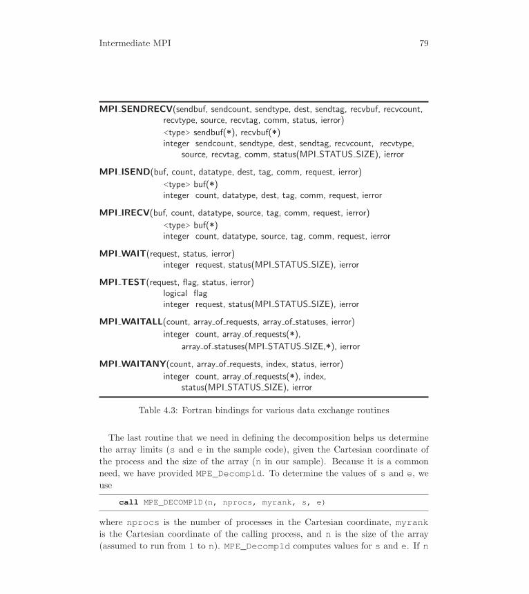
Intermediate MPI 79
MPI SENDRECV(sendbuf, sendcount, sendtype, dest, sendtag, recvbuf, recvcount,recvtype, source, recvtag, comm, status, ierror)
<type> sendbuf(*), recvbuf(*)integer sendcount, sendtype, dest, sendtag, recvcount, recvtype,
source, recvtag, comm, status(MPI STATUS SIZE), ierror
MPI ISEND(buf, count, datatype, dest, tag, comm, request, ierror)
<type> buf(*)integer count, datatype, dest, tag, comm, request, ierror
MPI IRECV(buf, count, datatype, source, tag, comm, request, ierror)
<type> buf(*)integer count, datatype, source, tag, comm, request, ierror
MPI WAIT(request, status, ierror)integer request, status(MPI STATUS SIZE), ierror
MPI TEST(request, flag, status, ierror)logical flaginteger request, status(MPI STATUS SIZE), ierror
MPI WAITALL(count, array of requests, array of statuses, ierror)
integer count, array of requests(*),
array of statuses(MPI STATUS SIZE,*), ierror
MPI WAITANY(count, array of requests, index, status, ierror)
integer count, array of requests(*), index,status(MPI STATUS SIZE), ierror
Table 4.3: Fortran bindings for various data exchange routines
The last routine that we need in defining the decomposition helps us determine
the array limits (s and e in the sample code), given the Cartesian coordinate of
the process and the size of the array (n in our sample). Because it is a common
need, we have provided MPE_Decomp1d. To determine the values of s and e, weuse
call MPE_DECOMP1D(n, nprocs, myrank, s, e)
where nprocs is the number of processes in the Cartesian coordinate, myrankis the Cartesian coordinate of the calling process, and n is the size of the array
(assumed to run from 1 to n). MPE_Decomp1d computes values for s and e. If n
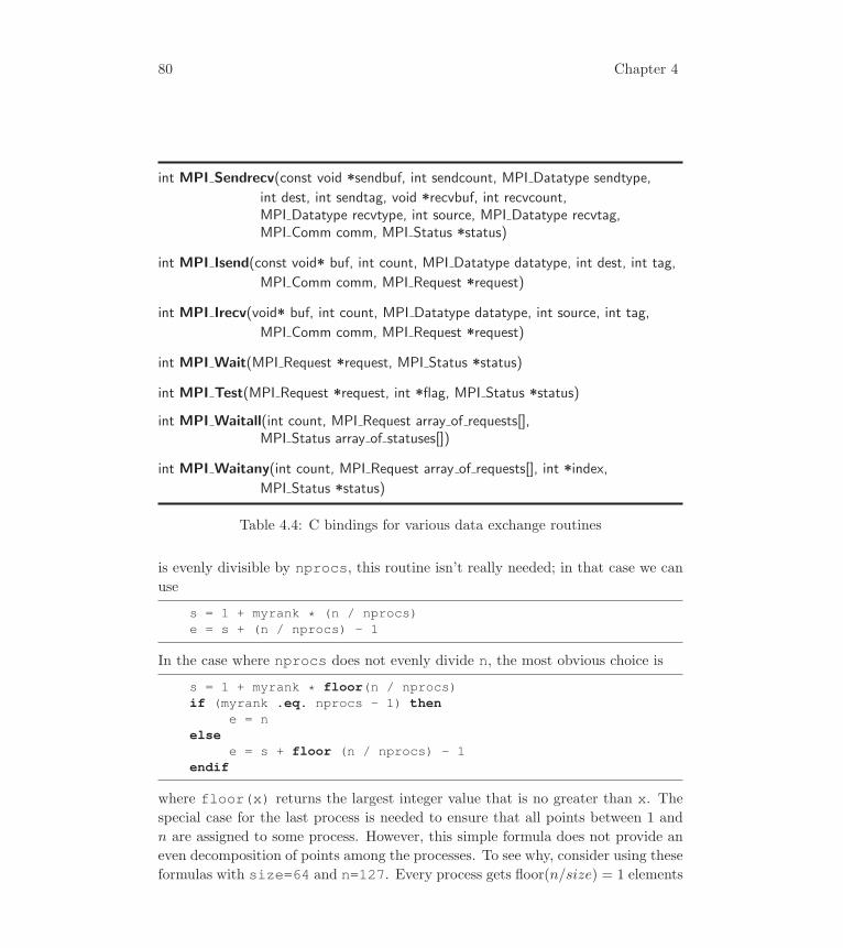
80 Chapter 4
int MPI Sendrecv(const void *sendbuf, int sendcount, MPI Datatype sendtype,
int dest, int sendtag, void *recvbuf, int recvcount,MPI Datatype recvtype, int source, MPI Datatype recvtag,MPI Comm comm, MPI Status *status)
int MPI Isend(const void* buf, int count, MPI Datatype datatype, int dest, int tag,
MPI Comm comm, MPI Request *request)
int MPI Irecv(void* buf, int count, MPI Datatype datatype, int source, int tag,
MPI Comm comm, MPI Request *request)
int MPI Wait(MPI Request *request, MPI Status *status)
int MPI Test(MPI Request *request, int *flag, MPI Status *status)
int MPI Waitall(int count, MPI Request array of requests[],MPI Status array of statuses[])
int MPI Waitany(int count, MPI Request array of requests[], int *index,
MPI Status *status)
Table 4.4: C bindings for various data exchange routines
is evenly divisible by nprocs, this routine isn’t really needed; in that case we can
use
s = 1 + myrank * (n / nprocs)e = s + (n / nprocs) - 1
In the case where nprocs does not evenly divide n, the most obvious choice is
s = 1 + myrank * floor(n / nprocs)if (myrank .eq. nprocs - 1) then
e = nelse
e = s + floor (n / nprocs) - 1endif
where floor(x) returns the largest integer value that is no greater than x. The
special case for the last process is needed to ensure that all points between 1 and
n are assigned to some process. However, this simple formula does not provide an
even decomposition of points among the processes. To see why, consider using these
formulas with size=64 and n=127. Every process gets floor(n/size) = 1 elements
Intermediate MPI 81
except for the last, which gets e − s + 1 = n − 63 ∗ floor(n/size) = 64 elements.
MPE_Decomp1d in this case gives processes 0 through 62 two elements and gives
the last process a single element. By using MPE_Decomp1d, we are ensured that
if nprocs does not evenly divide n, we will still get correct decomposition of the
data, with good load balancing.
Now that we know how the data is decomposed among the processes and how the
processes are ranked in the decomposition, we can write the routine to get the data
that we need. For each process, we must get the ghost-point data for the s-1 row
from the process below and the data for the e+1 row from the process above. Many
methods exist to do even this simple operation, and we will investigate several of
them through the course of this chapter.
4.3 A Code for the Poisson Problem
In this section we will assemble the pieces of the code that we have defined, as
well as the first version of the MPI routines needed to exchange the ghost points
between the processes.
The only piece of this code that we have not yet described is the routine to ex-
change data between the processes. The rest of this chapter will be concerned with
different ways to perform this communication operation, and it will pay particular
attention to some subtle issues that are often ignored in discussions of message
passing. With the warning that we are about to embark on a long journey, we start
with perhaps the simplest approach, shown in Figure 4.8.
In this routine, each process sends data to the process on top and then receives
data from the process below it. The order is then reversed, and data is sent to the
process below and received from the process above. We will see below that, while
this strategy is simple, it is not necessarily the best way to implement the exchange
of ghost points.
We now have all of the pieces needed to put together our first version of the
Poisson solver program. This program uses MPI_Cart_create to create the de-
composition of processes and the routine MPE_Decomp1d to determine the decom-
position of the arrays. The routine onedinit simply initializes the elements of
the arrays a, b, and f. The solution is computed alternately in the array a and
then b; this is why there are two calls to exchng1 and sweep1d in the loop. The
iteration is terminated when the difference between two successive approximations
to the solution is less than 1 × 10⁻⁵. The difference between the local parts of aand b is computed with the routine diff; the routine MPI_Allreduce is used
to ensure that all processes compute the same value for the difference in all of the

82 Chapter 4
subroutine exchng1(a, nx, s, e, comm1d, nbrbottom, nbrtop)use mpiinteger nx, s, e, comm1d, nbrbottom, nbrtopdouble precision a(0:nx+1,s-1:e+1)integer ierr
!call MPI_SEND(a(1,e), nx, MPI_DOUBLE_PRECISION, &
nbrtop, 0, comm1d, ierr)call MPI_RECV(a(1,s-1), nx, MPI_DOUBLE_PRECISION, &
nbrbottom, 0, comm1d, MPI_STATUS_IGNORE, ierr)call MPI_SEND(a(1,s), nx, MPI_DOUBLE_PRECISION, &
nbrbottom, 1, comm1d, ierr)call MPI_RECV(a(1,e+1), nx, MPI_DOUBLE_PRECISION, &
nbrtop, 1, comm1d, MPI_STATUS_IGNORE, ierr)returnend
Figure 4.8: Code to exchange data for ghost points using blocking sends and receives
elements. The program prints both the progress of the iterations and the final iter-
ation count. A do-loop with a maximum iteration count ensures that the program
terminates even if the iteration is not converging. The computational part of the
program is shown in Figure 4.9.
Let’s run this program, using the MPI profiling interface and the graphical tools
in order to understand the behavior. Using the “automatic” profiling method de-
scribed in Chapter 7, we use the MPE profiling files ‘mpe_proff.o’ and ‘mpe_-prof.o’ to generate a logfile of the communication. The ‘Makefile’ in the file
‘intermediate’ contains a target for ‘oned’; this is the first version of our Poisson
solver. To run it, we give the command
mpiexec -n 8 ./oned
Using the MPE logging tools described in Section 3.7.3, we can get a graphical
display of the communication. One output from upshot is shown in Figure 4.10.
Note that the communication is entirely sequential! What went wrong?
Although this is a frequently used communication pattern, it is not a safe one,
particularly for large values of nx (long messages). The reason is that the amount
of parallelism depends in a subtle way on the amount of buffering provided by
the message passing system, which is not explicitly specified by MPI and may be
difficult to determine. Let us suppose that we run this on a system with a small

Intermediate MPI 83
! Get a new communicator for a decomposition of the domain! and my position in it
call MPI_CART_CREATE(MPI_COMM_WORLD, 1, numprocs, .false., &.true., comm1d, ierr)
call MPI_COMM_RANK(comm1d, myid, ierr)call MPI_CART_SHIFT(comm1d, 0, 1, nbrbottom, nbrtop, ierr)
! Compute the actual decompositioncall MPE_DECOMP1D(ny, numprocs, myid, s, e)
! Initialize the right-hand-side (f) and the initial solution! guess (a)
call ONEDINIT(a, b, f, nx, s, e)!! Actually do the computation. Note the use of a collective! operation to check for convergence, and a do-loop to bound the! number of iterations.!
do it=1, maxit! get ghost points
call EXCHNG1(a, nx, s, e, comm1d, nbrbottom, nbrtop)! perform one Jacobi "sweep"
call SWEEP1D(a, f, nx, s, e, b)! repeat to get a solution back into array a
call EXCHNG1(b, nx, s, e, comm1d, nbrbottom, nbrtop)call SWEEP1D(b, f, nx, s, e, a)
! check for convergencediffw = DIFF(a, b, nx, s, e)call MPI_ALLREDUCE(diffw, diffnorm, 1, &
MPI_DOUBLE_PRECISION, &MPI_SUM, comm1d, ierr)
if (diffnorm .lt. 1.0e-5) exitif (myid .eq. 0) print *, 2*it, ’ Difference is ’, diffnorm
enddoif (myid .eq. 0 .and. it .gt. maxit) thenprint *, ’Failed to converge’
endifif (myid .eq. 0) thenprint *, ’Converged after ’, 2*it, ’ Iterations’
endif
Figure 4.9: Implementation of the Jacobi iteration

84 Chapter 4
���� ��� ���� ���� ���� ���� ���
��������� ������ ����� �� �� ���!
���� ����� � �� ���! ������ ����
�������! ����� ���� ��� ������
�����"
�
�
�
�
�
�
Figure 4.10: Communication in a single iteration for send followed by receive
amount of system buffer space or with a large message size. Then we will get the
behavior displayed in Figure 4.10.
Looking at the upshot output gives us a clue to what has happened. The sends
do not complete until the matching receives take place on the destination process.
Since one process (the “top” process) does not send to anyone in the first step, it
can receive from the process below it, thus allowing that process to receive from
below it, and so forth. This produces a staircase pattern of sends and receives. We
illustrate this in Figure 4.11.
Before we go any farther, we need to understand in more detail what happens
when we ask MPI to send a message.
Consider the following code:
if (rank .eq. 0) thencall MPI_Send(sbuffer, ..., 1, ...)
elsecall MPI_Recv(rbuffer, ..., 0, ...)
endif
What happens on the process with rank zero?
The easy answer is that the message in sbuffer is sent to process one. But
what if process one is not ready to receive it? Perhaps process one is still computing
a previous result. What can process zero do? Three possibilities exist: process zero
can stop and wait until process one is ready to receive the message, it can copy
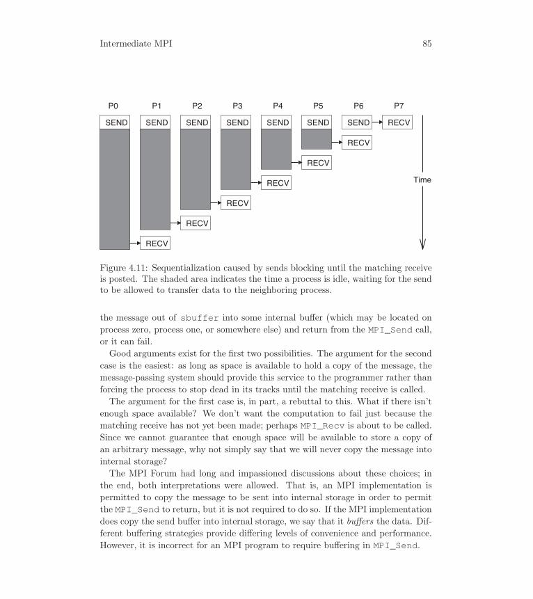
Intermediate MPI 85
SEND SEND SEND SEND SEND SEND SEND RECV
RECV
RECV
RECV
RECV
RECV
RECV
P0 P1 P2 P3 P4 P5 P6 P7
Time
Figure 4.11: Sequentialization caused by sends blocking until the matching receiveis posted. The shaded area indicates the time a process is idle, waiting for the sendto be allowed to transfer data to the neighboring process.
the message out of sbuffer into some internal buffer (which may be located on
process zero, process one, or somewhere else) and return from the MPI_Send call,
or it can fail.
Good arguments exist for the first two possibilities. The argument for the second
case is the easiest: as long as space is available to hold a copy of the message, the
message-passing system should provide this service to the programmer rather than
forcing the process to stop dead in its tracks until the matching receive is called.
The argument for the first case is, in part, a rebuttal to this. What if there isn’t
enough space available? We don’t want the computation to fail just because the
matching receive has not yet been made; perhaps MPI_Recv is about to be called.
Since we cannot guarantee that enough space will be available to store a copy of
an arbitrary message, why not simply say that we will never copy the message into
internal storage?
The MPI Forum had long and impassioned discussions about these choices; in
the end, both interpretations were allowed. That is, an MPI implementation is
permitted to copy the message to be sent into internal storage in order to permit
the MPI_Send to return, but it is not required to do so. If the MPI implementation
does copy the send buffer into internal storage, we say that it buffers the data. Dif-
ferent buffering strategies provide differing levels of convenience and performance.
However, it is incorrect for an MPI program to require buffering in MPI_Send.
86 Chapter 4
The third case is also interesting because it allows for certain performance im-
provements. The use of this kind of send operation is described in Section 7.1.5.
For large applications that are already using a large amount of memory, even
requiring the message-passing system to use all “available” memory may not provide
enough memory to make this code work. For example, consider a value of nx in
the above example that represents more memory space than is free on the process.
There is no place to store this message on the sending process; and, until the
receiver begins the matching receive, there is no place to store the message on the
receiving process. For large applications that are already using large amounts of
memory, the value of nx that triggers this situation may be quite small. Once the
receive is issued, however, we know that there is enough space to receive, since the
receiver supplies the buffer in the call to the receive.
The performance problem shown here is even more dangerous. As we saw, the
code runs (it does not deadlock) but it does not execute in parallel.
All of these issues suggest that programmers should be aware of the pitfalls in
assuming that the system will provide adequate buffering. In the next few sections,
we will describe ways in which the MPI programmer can ensure that the correct
parallel execution of a program does not depend on the amount of buffering, if any,
provided by the message-passing system.
Ordered send and receive. One of the easiest ways to correct for a dependence
on buffering is to order the sends and receives so that they are paired. That is,
the sends and receives are ordered so that if one process is sending to another, the
destination will do a receive that matches that send before doing a send of its own.
The code for this approach is shown in Figure 4.12. In this code, the even processes
(in Cartesian coordinates) send first, and the odd processes receive first.
Figure 4.13 shows the communication pattern in a single iteration of the Jacobi
code when using this approach.
Combined send and receive. Pairing the sends and receives is effective but
can be difficult to implement when the arrangement of processes is complex (for
example, with an irregular grid). An alternative is to use the MPI routine MPI_-Sendrecv. This routine allows you to send and receive data without worrying
about deadlock from a lack of buffering. Each process then sends to the process
below it and receives from the process above it. The code fragment for this sequence
of operations is shown in Figure 4.14. Note that we can use MPI_STATUS_IGNOREin MPI_Sendrecv as well as in MPI_Recv. In fact, MPI_STATUS_IGNORE may
be used anywhere that MPI uses a single status as an output parameter.

Intermediate MPI 87
subroutine exchng1(a, nx, s, e, comm1d, nbrbottom, nbrtop)use mpiinteger nx, s, e, comm1d, nbrbottom, nbrtopdouble precision a(0:nx+1,s-1:e+1)integer rank, coord, ierr
!call MPI_COMM_RANK(comm1d, rank, ierr)call MPI_CART_COORDS(comm1d, rank, 1, coord, ierr)if (mod(coord, 2) .eq. 0) then
call MPI_SEND(a(1,e), nx, MPI_DOUBLE_PRECISION, &nbrtop, 0, comm1d, ierr)
call MPI_RECV(a(1,s-1), nx, MPI_DOUBLE_PRECISION, &nbrbottom, 0, comm1d, MPI_STATUS_IGNORE, ierr)
call MPI_SEND(a(1,s), nx, MPI_DOUBLE_PRECISION, &nbrbottom, 1, comm1d, ierr)
call MPI_RECV(a(1,e+1), nx, MPI_DOUBLE_PRECISION, &nbrtop, 1, comm1d, MPI_STATUS_IGNORE, ierr)
elsecall MPI_RECV(a(1,s-1), nx, MPI_DOUBLE_PRECISION, &
nbrbottom, 0, comm1d, MPI_STATUS_IGNORE, ierr)call MPI_SEND(a(1,e), nx, MPI_DOUBLE_PRECISION, &
nbrtop, 0, comm1d, ierr)call MPI_RECV(a(1,e+1), nx, MPI_DOUBLE_PRECISION, &
nbrtop, 1, comm1d, MPI_STATUS_IGNORE, ierr)call MPI_SEND(a(1,s), nx, MPI_DOUBLE_PRECISION, &
nbrbottom, 1, comm1d, ierr)endifreturnend
Figure 4.12: Exchange routine with paired sends and receives

88 Chapter 4
��� ��� ��� �� ��� ��� ���
������� ���� �� ���� ������ ���#
����� ������ ����� ��# ���� ����
������# ����� ���� �� � �� ����
�� ���$
�
�
�
�
�
�
Figure 4.13: Communication in a single iteration with paired sends and receives
subroutine exchng1(a, nx, s, e, comm1d, nbrbottom, nbrtop)use mpiinteger nx, s, e, comm1d, nbrbottom, nbrtopdouble precision a(0:nx+1,s-1:e+1)integer ierr
!call MPI_SENDRECV( &
a(1,e), nx, MPI_DOUBLE_PRECISION, nbrtop, 0, &a(1,s-1), nx, MPI_DOUBLE_PRECISION, nbrbottom, 0,&comm1d, MPI_STATUS_IGNORE, ierr)
call MPI_SENDRECV( &a(1,s), nx, MPI_DOUBLE_PRECISION, nbrbottom, 1, &a(1,e+1), nx, MPI_DOUBLE_PRECISION, nbrtop, 1, &comm1d, MPI_STATUS_IGNORE, ierr)
returnend
Figure 4.14: Exchange routine with send-receive

Intermediate MPI 89
MPI BSEND(buf, count, datatype, dest, tag, comm, ierror)
<type> buf(*)integer count, datatype, dest, tag, comm, ierror
MPI BUFFER ATTACH(buffer, size, ierror)
<type> buffer(*)integer size, ierror
MPI BUFFER DETACH(buffer, size, ierror)
<type> buffer(*)integer size, ierror
Table 4.5: Fortran bindings for buffer operations
int MPI Bsend(const void* buf, int count, MPI Datatype datatype, int dest, int tag,MPI Comm comm)
int MPI Buffer attach(void* buffer, int size)
int MPI Buffer detach(void* buffer, int* size)
Table 4.6: C bindings for buffering routines. Note that even though the bufferargument in MPI_Buffer_detach is typed as void *, it is really a pointer to apointer and is typed as void * to simplify its use.
Buffered sends. Instead of requiring the programmer to determine a safe order-
ing of the send and receive operations, MPI allows the programmer to provide a
buffer into which data can be placed until it is delivered (or at least left the buffer).
The change to the exchange routine is simple; one just replaces the MPI_Send calls
with MPI_Bsend. The resulting routine is shown in Figure 4.15.
In addition to the change to the exchange routine, MPI requires that the pro-
grammer provide the storage into which the message may be placed with the routine
MPI_Buffer_attach. This buffer should be large enough to hold all of the mes-
sages that must be sent before the matching receives are called. In our case, we
need a buffer of 2*nx double precision values. We can provide this with code like
the following:
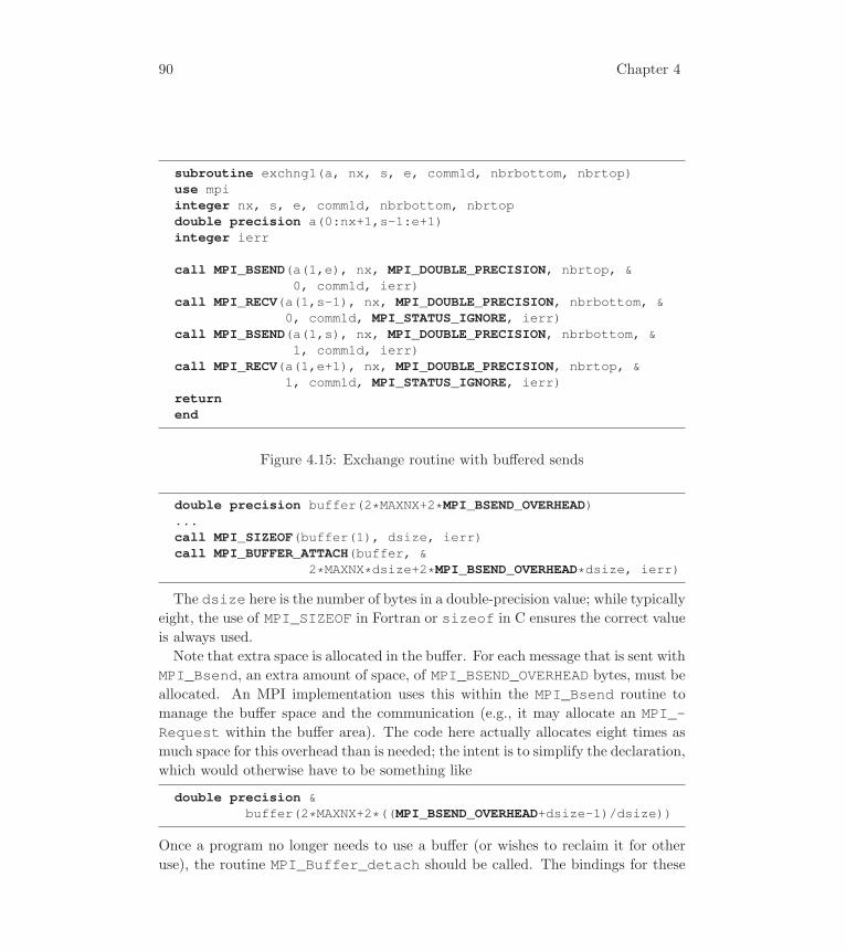
90 Chapter 4
subroutine exchng1(a, nx, s, e, comm1d, nbrbottom, nbrtop)use mpiinteger nx, s, e, comm1d, nbrbottom, nbrtopdouble precision a(0:nx+1,s-1:e+1)integer ierr
call MPI_BSEND(a(1,e), nx, MPI_DOUBLE_PRECISION, nbrtop, &0, comm1d, ierr)
call MPI_RECV(a(1,s-1), nx, MPI_DOUBLE_PRECISION, nbrbottom, &0, comm1d, MPI_STATUS_IGNORE, ierr)
call MPI_BSEND(a(1,s), nx, MPI_DOUBLE_PRECISION, nbrbottom, &1, comm1d, ierr)
call MPI_RECV(a(1,e+1), nx, MPI_DOUBLE_PRECISION, nbrtop, &1, comm1d, MPI_STATUS_IGNORE, ierr)
returnend
Figure 4.15: Exchange routine with buffered sends
double precision buffer(2*MAXNX+2*MPI_BSEND_OVERHEAD)...call MPI_SIZEOF(buffer(1), dsize, ierr)call MPI_BUFFER_ATTACH(buffer, &
2*MAXNX*dsize+2*MPI_BSEND_OVERHEAD*dsize, ierr)
The dsize here is the number of bytes in a double-precision value; while typically
eight, the use of MPI_SIZEOF in Fortran or sizeof in C ensures the correct value
is always used.
Note that extra space is allocated in the buffer. For each message that is sent with
MPI_Bsend, an extra amount of space, of MPI_BSEND_OVERHEAD bytes, must be
allocated. An MPI implementation uses this within the MPI_Bsend routine to
manage the buffer space and the communication (e.g., it may allocate an MPI_-Request within the buffer area). The code here actually allocates eight times as
much space for this overhead than is needed; the intent is to simplify the declaration,
which would otherwise have to be something like
double precision &buffer(2*MAXNX+2*((MPI_BSEND_OVERHEAD+dsize-1)/dsize))
Once a program no longer needs to use a buffer (or wishes to reclaim it for other
use), the routine MPI_Buffer_detach should be called. The bindings for these

Intermediate MPI 91
routines are shown in Tables 4.5 and 4.6. (The reason for the buffer and sizearguments in MPI_Buffer_detach is that C programmers can use these to find
out the location and size of an existing buffer in order to free it.) We emphasize
that buffering may incur a performance penalty (extra effort copying data to and
from the buffer) and may expose the program to failure if the amount of needed
buffering is not calculated correctly.
One final caution when using MPI_Bsend is needed. One might think that a
loop like the following could be used to send 100 bytes at each iteration of the loop:
size = 100 + MPI_BSEND_OVERHEADcall MPI_BUFFER_ATTACH(buf, size, ierr)do i=1, n
call MPI_BSEND(sbuf, 100, MPI_BYTE, 0, dest, &MPI_COMM_WORLD, ierr)
< ... other work>enddocall MPI_BUFFER_DETACH(buf, size, ierr)
The problem with this code is the message sent in the ith step of the loop may not
have been delivered when the next call to MPI_Bsend occurs in the i + 1st step.
To use MPI_Bsend correctly in this case, either the buffer given specified with
MPI_Buffer_attach must be large enough to hold all of the data sent (in this
case, n ∗ (100+MPI_BSEND_OVERHEAD)), or the buffer attach and detach must be
moved inside of the loop (at the cost of extra overhead).
An alternative to using the buffered send involves using communications opera-
tions that do not block but permit the program to continue to execute instead of
waiting for communications to complete. This approach also allows the program to
compute while waiting for the communications to complete. However, the ability
to overlap computation with communication is only one reason to consider the non-
blocking operations in MPI; the ability to prevent one communication operation
from preventing others from finishing is just as important.
4.4 Using Nonblocking Communications
On most parallel computers, moving data from one process to another takes more
time than moving or manipulating data within a single process. For example, on
one modern parallel computer, each processor core can compute over 10 billion
floating-point results per second but can only move roughly two hundred million

92 Chapter 4
words per second between processes.2 To keep a program from being slowed (also
described as “starved for data”), many parallel computers allow users to start
sending (and receiving) several messages and to proceed with other operations.
Programmers who have used “asynchronous I/O” will recognize this approach as a
way of compensating for the relatively slow speed of access to external information
(disks in the case of I/O, another process in the case of message passing). MPI
supports this approach by providing nonblocking sends and receives.
Nonblocking routines also solve the problem of buffering, by providing a way to
defer completion of communication until the user, through an MPI receive opera-
tion, provides a place for a message to be received into. Many MPI concepts have
this property of solving two or more problems.
The routine MPI_Isend begins the nonblocking send operation. The arguments
are the same as for MPI_Send with the addition of a handle as the next to last
argument (the last argument in C). The two routines also behave similarly except
that, for MPI_Isend, the buffer containing the message to be sent must not be
modified until the message has been delivered (more precisely, until the operation
is complete, as indicated by one of the MPI_Wait or MPI_Test routines). In C,
the type of this handle is MPI_Request. In the new Fortran 2008 binding, which
we discuss in Using Advanced MPI [55], the type is similar to C: Type(MPI_-Request). Because the Fortran 2008 types are similar to C, we won’t mention
them in the rest of the discussions; see Chapter 11 of Using Advanced MPI [55] or
the MPI-3 standard [94] for more information.
The handle argument is used to determine whether an operation has completed.
The easiest way to test is with MPI_Test:
call MPI_ISEND(buffer, count, datatype, dest, tag, &comm, request, ierr)
< do other work >flag = .false.do while (.not. flag)
call MPI_TEST(request, flag, status, ierr)enddo
Often, one wishes to wait until the send completes. Rather than writing the loop
in the previous example, one can use MPI_Wait instead:
call MPI_WAIT(request, status, ierr)
2This apparent mismatch of capabilities reflects underlying engineering and physical realitiesand is a major reason that the message-passing approach, which keeps the programmer remindedof the cost of accessing remote data, has been a successful way to program parallel computers.

Intermediate MPI 93
Once a nonblocking operation is complete (e.g., MPI_Wait returns or MPI_Testreturns with flag = .true.), the request is set to MPI_REQUEST_NULL.
The routine MPI_Irecv begins the nonblocking receive operation. It has one
additional argument, the handle, just as MPI_Isend does. It also has one less
argument: the status argument, which is used to return information on the com-
pleted receive, is deleted from the argument list. Just as for MPI_Isend, MPI_-Test may be used to test for the completion of a receive started with MPI_Irecv,and MPI_Wait may be used to wait for the completion of such a receive. The
status arguments of these two routines return the information on the completed
receive in the same form as MPI_Recv does for a blocking receive.
In many cases, one wishes to test or wait for many nonblocking operations. Al-
though one can simply loop through the operations, this approach is inefficient,
since this forces the user’s program to be constantly executing rather than waiting
(possibly without consuming CPU time) for the “next” message. MPI provides a
way to wait for all or any of a collection of nonblocking operations (with MPI_-Waitall and MPI_Waitany) and to test all or any of a collection of nonblocking
operations (with MPI_Testall and MPI_Testany). For example, to start two
nonblocking receives and then wait on them, one can use
call MPI_IRECV(..., requests(1), ierr)call MPI_IRECV(..., requests(2), ierr)...call MPI_WAITALL(2, requests, status, ierr)
Here, status must be an array of two MPI_status objects; it can be declared
with
integer status(MPI_STATUS_SIZE,2)
Alternatively, if the values in the statuses array are not required, one can
use the value MPI_STATUSES_IGNORE instead for the statuses output param-
eters. This special value may be used anywhere an array of statuses is an output
parameter.
With these routines, we can rewrite the exchange routine exchng1 using non-
blocking operations, as shown in Figure 4.16. This approach allows for both sends
and receives to take place at the same time. In principle, this approach can be al-
most twice as fast as the version in Figure 4.12, though not all systems support this
(don’t forget that MPI was designed to support current and future message-passing
systems). In the next section, we try them out and see what happens.

94 Chapter 4
subroutine exchng1(a, nx, s, e, comm1d, nbrbottom, nbrtop)use mpiinteger nx, s, e, comm1d, nbrbottom, nbrtopdouble precision a(0:nx+1,s-1:e+1)integer ierr, req(4)
!call MPI_IRECV(&
a(1,s-1), nx, MPI_DOUBLE_PRECISION, nbrbottom, 0, &comm1d, req(1), ierr)
call MPI_IRECV(&a(1,e+1), nx, MPI_DOUBLE_PRECISION, nbrtop, 1, &comm1d, req(2), ierr)
call MPI_ISEND(&a(1,e), nx, MPI_DOUBLE_PRECISION, nbrtop, 0, &comm1d, req(3), ierr)
call MPI_ISEND(&a(1,s), nx, MPI_DOUBLE_PRECISION, nbrbottom, 1, &comm1d, req(4), ierr)
!call MPI_WAITALL(4, req, MPI_STATUSES_IGNORE, ierr)returnend
Figure 4.16: Row-exchange routine using nonblocking operations
Note that in order to overlap communication and computation, we must make
further changes to our program. In particular, we need to change the sweepprogram to allow us to do some of the work while we wait for data to arrive. We will
come back to nonblocking operations in Section 4.9, where we discuss overlapping
communication with computation.
4.5 Synchronous Sends and “Safe” Programs
What can we do to ensure that a program does not depend on buffering? In general,
this is equivalent to the Turing halting-problem and is hence unanswerable, but in
many special cases it is possible to show that if the program runs successfully with
no buffering, it will run with any amount of buffering. MPI provides a way to
send a message so that the send does not return until the destination begins to
receive the message (in addition, just like MPI_Send, it doesn’t return until the
send buffer is available for reuse by the programmer). The routine is MPI_Ssend.
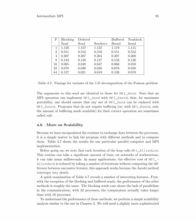
Intermediate MPI 95
P Blocking Ordered Buffered NonblockSend Send Sendrecv Bsend Isend
1 1.120 1.127 1.122 1.119 1.1152 0.551 0.552 0.559 0.551 0.5524 0.307 0.307 0.304 0.307 0.3088 0.133 0.128 0.127 0.133 0.12616 0.065 0.049 0.047 0.066 0.05032 0.078 0.036 0.028 0.078 0.02864 0.127 0.021 0.019 0.126 0.019
Table 4.7: Timings for variants of the 1-D decomposition of the Poisson problem
The arguments to this send are identical to those for MPI_Send. Note that an
MPI operation can implement MPI_Send with MPI_Ssend; thus, for maximum
portability, one should ensure that any use of MPI_Send can be replaced with
MPI_Ssend. Programs that do not require buffering (or, with MPI_Bsend, onlythe amount of buffering made available) for their correct operation are sometimes
called safe.
4.6 More on Scalability
Because we have encapsulated the routines to exchange data between the processes,
it is a simple matter to link the program with different methods and to compare
them. Table 4.7 shows the results for one particular parallel computer and MPI
implementation.
Before going on, we note that each iteration of the loop calls MPI_Allreduce.This routine can take a significant amount of time; on networks of workstations,
it can take many milliseconds. In many applications, the effective cost of MPI_-Allreduce is reduced by taking a number of iterations without computing the dif-
ference between successive iterates; this approach works because the Jacobi method
converges very slowly.
A quick examination of Table 4.7 reveals a number of interesting features. First,
with the exception of the blocking and buffered sends, the performance of the other
methods is roughly the same. The blocking sends case shows the lack of parallelism
in the communication; with 32 processes, the computation actually takes longer
than with 16 processes.
To understand the performance of these methods, we perform a simple scalability
analysis similar to the one in Chapter 3. We will need a slightly more sophisticated

96 Chapter 4
��
�������
������
�������
������
�������
������
�������
��� �� �� ��� ���� ����
� �
�
���������
������
�������
Figure 4.17: Predicted time for a 1-D (solid) and 2-D (dashed) decomposition of the2-D Poisson problem. The cost assuming no communication is also shown (dotted).
model of communication cost here. There, we used Tcomm as the time to send a
word. We will replace Tcomm with s+ rn as the time to send n bytes; for n large,
we have Tcomm ≈ r∗n. The term s is the latency or startup time; it can be thought
of as the time to send a message containing no data beyond the message tag and
source. The term r is the inverse rate; it is the time to send a single byte and is
given by one over the bandwidth. For example, if the bandwidth of a connection
is 1 GB/sec, r = 1/(1GB/sec) = 10−9 sec/byte. Using this formula, we can easily
see that the exchng1d routine in Figure 4.12 takes roughly 2(s+ rn) time, where
n = 8nx (assuming 8-byte double-precision data).
In a two-dimensional decomposition, let there be px processes in the x direction
and py processes in the y direction, with each process having the same number of
mesh points. Then, with the exception of the processes on any edge of the domain,
the amount of communication Tc is
Tc = 2
(s+ r
n
px
)+ 2
(s+ r
n
py
).

Intermediate MPI 97
If px = py =√p, this takes a particularly simple form:
Tc = 4
(s+ r
n√p
).
Figure 4.17 shows the expected performance for both 1-D and 2-D decompositions
of the domain, based on these estimates. The
The situation is even more extreme in 3-D, as shown in Figure 4.18. Care must
be exercised here because our analysis is good in the 3-D case only for p ≥ 27: the
reason is that for p < 27 no process has neighbors on all six sides, since the 3-D
decomposition creates smaller cubes in the domain.
Another way to look at the performance of a program is to compute the speedup
and parallel efficiency . The speedup is defined as
speedup =Time with no parallelism
Time with parallelism,
and the parallel efficiency is defined is speedup/p. For example, for the 1-D decom-
position, we have
speedup =fn2
fn2
p + 2(s+ rn)
efficiency =fn2
p(
fn2
p + 2(s+ rn))
=fn2
fn2 + 2(s+ rn)p
=1
1 + 2(s+rn)pfn2
.
Here, f is the cost of the floating-point computation at each mesh point, and r
is the cost to communicate each word. We can see that the efficiency is always
less than one. It improves as n increases and decreases as p increases. A similar
analysis can be carried out with a 2-D decomposition, which reveals the benefits of
this more complex decomposition for large numbers of processes. This is illustrated
in Figure 4.19, which shows plots of the parallel efficiencies for a range of both
process count p and mesh size n for the 1-D and 2-D decompositions. Note that
the 1-D decomposition has low efficiencies for large numbers of processes, while the
2-D decomposition has reasonable efficiencies for 10, 000 processes on suitable large
meshes.
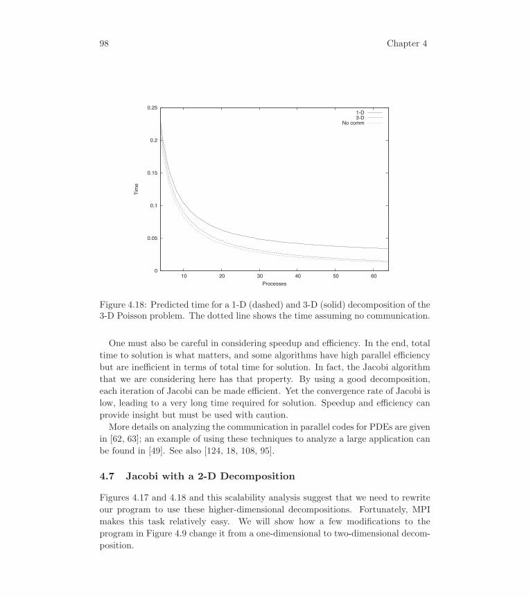
98 Chapter 4
��
�����
����
�����
����
�����
��� ��� ��� �� ��� ��
����
�����
������
������
Figure 4.18: Predicted time for a 1-D (dashed) and 3-D (solid) decomposition of the3-D Poisson problem. The dotted line shows the time assuming no communication.
One must also be careful in considering speedup and efficiency. In the end, total
time to solution is what matters, and some algorithms have high parallel efficiency
but are inefficient in terms of total time for solution. In fact, the Jacobi algorithm
that we are considering here has that property. By using a good decomposition,
each iteration of Jacobi can be made efficient. Yet the convergence rate of Jacobi is
low, leading to a very long time required for solution. Speedup and efficiency can
provide insight but must be used with caution.
More details on analyzing the communication in parallel codes for PDEs are given
in [62, 63]; an example of using these techniques to analyze a large application can
be found in [49]. See also [124, 18, 108, 95].
4.7 Jacobi with a 2-D Decomposition
Figures 4.17 and 4.18 and this scalability analysis suggest that we need to rewrite
our program to use these higher-dimensional decompositions. Fortunately, MPI
makes this task relatively easy. We will show how a few modifications to the
program in Figure 4.9 change it from a one-dimensional to two-dimensional decom-
position.
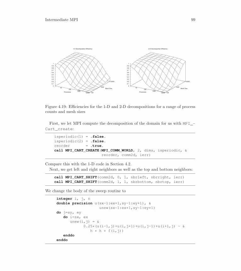
Intermediate MPI 99
����������������������������
�������
������������!������� ����
�����
������
�����"�
��
����
����
����
���
����
���
����
����
���
��
����������������������������
�������
������������!������� ����
�����
������
�����"�
��
����
����
����
���
����
���
����
����
���
��
Figure 4.19: Efficiencies for the 1-D and 2-D decompositions for a range of processcounts and mesh sizes
First, we let MPI compute the decomposition of the domain for us with MPI_-Cart_create:
isperiodic(1) = .false.isperiodic(2) = .false.reorder = .true.call MPI_CART_CREATE(MPI_COMM_WORLD, 2, dims, isperiodic, &
reorder, comm2d, ierr)
Compare this with the 1-D code in Section 4.2.
Next, we get left and right neighbors as well as the top and bottom neighbors:
call MPI_CART_SHIFT(comm2d, 0, 1, nbrleft, nbrright, ierr)call MPI_CART_SHIFT(comm2d, 1, 1, nbrbottom, nbrtop, ierr)
We change the body of the sweep routine to
integer i, j, ndouble precision u(sx-1:ex+1,sy-1:ey+1), &
unew(sx-1:ex+1,sy-1:ey+1)do j=sy, ey
do i=sx, exunew(i,j) = &
0.25*(u(i-1,j)+u(i,j+1)+u(i,j-1)+u(i+1,j) - &h * h * f(i,j))
enddoenddo
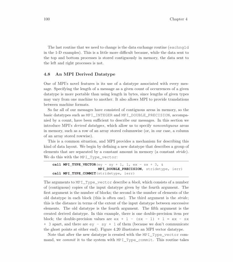
100 Chapter 4
The last routine that we need to change is the data exchange routine (exchng1din the 1-D examples). This is a little more difficult because, while the data sent to
the top and bottom processes is stored contiguously in memory, the data sent to
the left and right processes is not.
4.8 An MPI Derived Datatype
One of MPI’s novel features is its use of a datatype associated with every mes-
sage. Specifying the length of a message as a given count of occurrences of a given
datatype is more portable than using length in bytes, since lengths of given types
may vary from one machine to another. It also allows MPI to provide translations
between machine formats.
So far all of our messages have consisted of contiguous areas in memory, so the
basic datatypes such as MPI_INTEGER and MPI_DOUBLE_PRECISION, accompa-
nied by a count, have been sufficient to describe our messages. In this section we
introduce MPI’s derived datatypes, which allow us to specify noncontiguous areas
in memory, such as a row of an array stored columnwise (or, in our case, a column
of an array stored rowwise).
This is a common situation, and MPI provides a mechanism for describing this
kind of data layout. We begin by defining a new datatype that describes a group of
elements that are separated by a constant amount in memory (a constant stride).
We do this with the MPI_Type_vector:
call MPI_TYPE_VECTOR(ey - sy + 1, 1, ex - sx + 3, &MPI_DOUBLE_PRECISION, stridetype, ierr)
call MPI_TYPE_COMMIT(stridetype, ierr)
The arguments to MPI_Type_vector describe a block, which consists of a number
of (contiguous) copies of the input datatype given by the fourth argument. The
first argument is the number of blocks; the second is the number of elements of the
old datatype in each block (this is often one). The third argument is the stride;
this is the distance in terms of the extent of the input datatype between successive
elements. The old datatype is the fourth argument. The fifth argument is the
created derived datatype. In this example, there is one double-precision item per
block; the double-precision values are ex + 1 - (sx - 1) + 1 = ex - sx+ 3 apart, and there are ey - sy + 1 of them (because we don’t communicate
the ghost points at either end). Figure 4.20 illustrates an MPI vector datatype.
Note that after the new datatype is created with the MPI_Type_vector com-
mand, we commit it to the system with MPI_Type_commit. This routine takes

Intermediate MPI 101
1 2 3 4 5 6 7
8 9 10 11 12 13 14
15 16 17 18 19 20 21
22 23 24 25 26 27 28
29 30 31 32 33 34 35
MPI_TYPE_VECTOR(5, 1, 7, MPI_DOUBLE_PRECISION, newtype,ierr)
Figure 4.20: A strided data item (shaded) and its MPI definition. Numbers indicateconsecutive memory locations.
the newly constructed datatype and gives the system the opportunity to perform
any performance optimizations that it may wish. All user-constructed data types
must be committed before they can be used.
With this new datatype definition, the MPI code for sending a row differs from
the code for sending a column only in the datatype argument. The final version of
exchng2d is shown in Figure 4.21.
When a datatype is no longer needed, it should be freed with MPI_Type_-free. The datatype variable (the first argument) is set to MPI_TYPE_NULL by
MPI_Type_free. Bindings for these routines are shown in Tables 4.8 and 4.9.
An alternative definition of the strided type, described in Section 5.4, allows the
programmer to send any number of elements with the same datatype.
4.9 Overlapping Communication and Computation
Because to moving data from one process to another can be time-consuming, it is
often advantageous to arrange the program so that some work can be done while
the messages are “in transit.” So far, we have used nonblocking operations to avoid
deadlock in the communications. Here we describe some of the details in arranging
a program so that computation and communication can take place simultaneously.
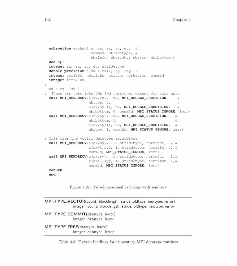
102 Chapter 4
subroutine exchng2(a, sx, ex, sy, ey, &comm2d, stridetype, &nbrleft, nbrright, nbrtop, nbrbottom )
use mpiinteger sx, ex, sy, ey, stridetypedouble precision a(sx-1:ex+1, sy-1:ey+1)integer nbrleft, nbrright, nbrtop, nbrbottom, comm2dinteger ierr, nx
!nx = ex - sx + 1
! These are just like the 1-d versions, except for less datacall MPI_SENDRECV(a(sx,ey), nx, MPI_DOUBLE_PRECISION, &
nbrtop, 0, &a(sx,sy-1), nx, MPI_DOUBLE_PRECISION, &nbrbottom, 0, comm2d, MPI_STATUS_IGNORE, ierr)
call MPI_SENDRECV(a(sx,sy), nx, MPI_DOUBLE_PRECISION, &nbrbottom, 1, &a(sx,ey+1), nx, MPI_DOUBLE_PRECISION, &nbrtop, 1, comm2d, MPI_STATUS_IGNORE, ierr)
!! This uses the vector datatype stridetype
call MPI_SENDRECV(a(ex,sy), 1, stridetype, nbrright, 0, &a(sx-1,sy), 1, stridetype, nbrleft, 0, &comm2d, MPI_STATUS_IGNORE, ierr)
call MPI_SENDRECV(a(sx,sy), 1, stridetype, nbrleft, 1,&a(ex+1,sy), 1, stridetype, nbrright, 1,&comm2d, MPI_STATUS_IGNORE, ierr)
returnend
Figure 4.21: Two-dimensional exchange with sendrecv
MPI TYPE VECTOR(count, blocklength, stride, oldtype, newtype, ierror)integer count, blocklength, stride, oldtype, newtype, ierror
MPI TYPE COMMIT(datatype, ierror)integer datatype, ierror
MPI TYPE FREE(datatype, ierror)integer datatype, ierror
Table 4.8: Fortran bindings for elementary MPI datatype routines
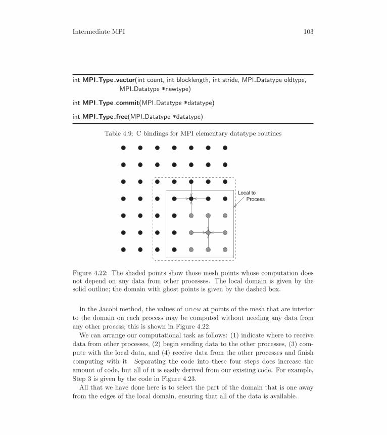
Intermediate MPI 103
int MPI Type vector(int count, int blocklength, int stride, MPI Datatype oldtype,
MPI Datatype *newtype)
int MPI Type commit(MPI Datatype *datatype)
int MPI Type free(MPI Datatype *datatype)
Table 4.9: C bindings for MPI elementary datatype routines
Local toProcess
Figure 4.22: The shaded points show those mesh points whose computation doesnot depend on any data from other processes. The local domain is given by thesolid outline; the domain with ghost points is given by the dashed box.
In the Jacobi method, the values of unew at points of the mesh that are interior
to the domain on each process may be computed without needing any data from
any other process; this is shown in Figure 4.22.
We can arrange our computational task as follows: (1) indicate where to receive
data from other processes, (2) begin sending data to the other processes, (3) com-
pute with the local data, and (4) receive data from the other processes and finish
computing with it. Separating the code into these four steps does increase the
amount of code, but all of it is easily derived from our existing code. For example,
Step 3 is given by the code in Figure 4.23.
All that we have done here is to select the part of the domain that is one away
from the edges of the local domain, ensuring that all of the data is available.

104 Chapter 4
integer i, j, ndouble precision u(sx-1:ex+1,sy-1:ey+1), &
unew(sx-1:ex+1,sy-1:ey+1)do j=sy+1, ey-1
do i=sx+1, ex-1unew(i,j) = &
0.25*(u(i-1,j)+u(i,j+1)+u(i,j-1)+u(i+1,j) - &h * h * f(i,j))
enddoenddo
Figure 4.23: Code to compute a Jacobi iteration with only local data
The communication routines change in similar ways; in addition, the calls are
split into two sections of code, separated by the main computational section. The
first part begins both the nonblocking sends and nonblocking receives:
call MPI_IRECV(..., requests(1), ierr)...call MPI_ISEND(..., requests(5), ierr)
These are followed by
do k=1,8call MPI_WAITANY(8, requests, idx, status, ierr)! Use tag to determine which edgeselect case (status(MPI_TAG))
case(1)do j=sy,ey
unew(si,j) = ...enddocase(2)do j=sy,ey
unew(ei,j) = ...enddocase(3)do i=sx,ex
unew(i,ej) = ...enddocase(100)do i=sx,ex
unew(i,sj) = ...enddo
Intermediate MPI 105
end selectenddo
Here, requests(1) through requests(4) are receive handles; requests(5)through requests(8) are send handles.
4.10 More on Timing Programs
Our simple code can also be used to solve time-dependent PDEs. Many discretiza-
tions for time-dependent PDEs require only the data that our Jacobi iteration needs.
The only difference is that the sweep routines change and there is no longer any
need for MPI_Allreduce to check for convergence. However, this does raise an
issue when timing this program: how do we know that every process is finished
when we call MPI_Wtime? We can use the MPI routine MPI_Barrier to ensure
that every process has completed the computation. A barrier is a special collective
operation that does not let the calling process continue until all processes in the
communicator have called MPI_Barrier.
call MPI_Barrier(MPI_COMM_WORLD, ierr)t1 = MPI_Wtime()<do work>call MPI_Barrier(MPI_COMM_WORLD, ierr)total_time = MPI_Wtime() - t1
The barriers ensure that all processes have reached the same point in the code and
are ready to proceed. Many of the collective operations (e.g., MPI_Allreduce)have the same property; that is, no process can exit the operation until all processes
have entered. Note that this is not true for operations like MPI_Reduce, whereonly the root process must wait for all other processes to enter the MPI_Reducecall. The bindings for MPI_Barrier are shown in Tables 4.10 and 4.11.
This simple timing code is in fact often too simple. A number of factors can
cause this code to produce misleading results. One well-known problem is that of
cache: if the data needed for the work step will fit into cache, the first time this
data is accessed, the time will often be dominated not by the work itself but by
the time to load the data into cache. A less well-known but related problem is
the demand-loading of code: in many systems, the machine instructions are not
loaded from disk into memory until they are first referenced. Because this requires
accessing a disk (or at least a remote file server), this can take a significant amount
of time. Thus, it is better to use a loop such as the following:

106 Chapter 4
MPI BARRIER(comm, ierr)integer comm, ierr
Table 4.10: Fortran bindings for barrier routine
int MPI Barrier(MPI Comm comm)
Table 4.11: C binding for barrier routine
do i=1,2call MPI_Barrier(MPI_COMM_WORLD, ierr)t1 = MPI_Wtime()<do work>call MPI_Barrier(MPI_COMM_WORLD, ierr)total_time = MPI_Wtime() - t1
enddo
This simple code runs the test twice, discarding the result from the first test. More
sophisticated testing methods are discussed in [66]. The chapter on measuring
performance in [24] also contains valuable suggestions for accurately timing tests.
Note that this code is only approximate. There is no guarantee that all processes
will exit the MPI_Barrier at even approximately the same time. The MPI_-Barrier guarantees only that no process exits before all have entered. If you
really need a way to have all processes synchronized in time, a method is described
in [126] that was used for benchmarking collective communications in MPI.
4.11 Three Dimensions
So far, we have restricted ourselves to the 2-D problem. Now, we want to introduce
the 3-D case and also show the problem in a C implementation. Even a relatively
small 3-D problem having 100 grid points on a side involves 106 grid points; it is
common to encounter two or three orders of magnitude more grid points than this
in 3-D simulations. These problems are consequently ideal candidates for parallel
computing. The flexibility of MPI makes generalizing our previous 2-D problem
solutions to 3-D straightforward.
One complication in developing a 3-D code is the decomposition of the domain
among the processes. As we would expect from the scalability analysis in this
chapter, we should use a 3-D virtual topology. MPI provides the routine MPI_-
Intermediate MPI 107
MPI DIMS CREATE(nnodes, ndims, dims, ierr)
integer nnodes, ndims, dims(*), ierr
Table 4.12: Fortran binding for MPI_DIMS_CREATE
int MPI Dims create(int nnodes, int ndims, int dims[])
Table 4.13: C binding for MPI_DIMS_CREATE
Dims_create to aid in generating a Cartesian virtual topology with any number
of dimensions. This routine takes as input the total number of processes and the
number of dimensions, and it returns an array containing the Cartesian dimensions.
These values may be used as the dims argument to MPI_Cart_create. The
bindings are shown in Tables 4.12 and 4.13.
4.12 Common Errors and Misunderstandings
As in the preceding chapter, we list a few common pitfalls associated with the
concepts presented in this one.
Not making programs safe. In Section 4.5 we identified the concept of “safe”
programs; those that would still work if all blocking sends were replaced by syn-
chronous sends. A program of the following form is inherently unsafe:
Process 0 Process 1MPI_Send to process 1 MPI_Send to process 0MPI_Recv from process 1 MPI_Recv from process 0
It is certain to fail for some value of the length of the message, since there will not
be enough system buffering for both messages to be copied out of the send buffers
before being copied into the receive buffers. Many implementations have generous
buffering, which can lull the programmer into a false sense of security. As messages
get bigger, eventually the buffer limit will be reached and the program will fail.
When exchanging messages between processes, it is better to write a safe program
using one of the techniques described in this chapter.
• Interleave sends and receives so that one process is sending while the other is
receiving.
• Use MPI_Sendrecv.

108 Chapter 4
• Allocate one’s own buffers with MPI_Buffer_attach.
• Use the nonblocking operations MPI_Isend and MPI_Irecv.
The most common and general approach is the last one.
Counting on the overlapping of communication and computation. The
nonblocking operations are more important for allowing safe programs than for im-
proving performance by overlapping communication and computation. Although
we described in Section 4.9 how to structure our program to allow for such over-
lapping, many implementations cannot overlap without extra hardware in the form
of a communication coprocessor. Use of the nonblocking operations allows an im-
plementation to obtain extra performance by simultaneously communicating and
computing, but it is not required to; and whether such overlapping is possible
may depend on the hardware environment. If switching to nonblocking operations
doesn’t improve performance, it may not be your fault.
4.13 Application: Nek5000/NekCEM
Nek5000/NekCEM are scalable open-source codes for computational fluid dynam-
ics (Nek5000) and computational electromagnetics (NekCEM) used in a variety
of applications including vascular flow, heat transfer, combustion, ocean model-
ing, fundamentals of turbulence, astrophysics, accelerator physics, and nanopho-
tonics. The codes are based on spectral element methods (SEMs) coupled with
high-order timestepping to solve the governing initial-/boundary-value problems in
two or three space dimensions and time. Nek5000 solves the incompressible Navier-
Stokes equations (or a low-Mach variant) and NekCEM solves the time-dependent
Maxwell’s equations. The principal design goal for Nek5000/NekCEM is to reduce
the number of gridpoints through the use of high-order methods while maintaining
a cost-per-gridpoint comparable to low-order methods. Because of its minimal nu-
merical dispersion, the benefits of the SEM are manifest for problems where long
time-integration is required, which is often the case in high-performance comput-
ing applications that are striving to capture significant scale interactions spanning
several decades.
In the SEM, the computational domain is represented as the union of E nonover-
lapping elements, where the elements are typically curvilinear hexahedra (bricks).
Within each element, the solution and data are represented as Nth-order tensor-
product polynomials.

Intermediate MPI 109
The SEM has much in common with the finite element method (FEM) save
that, through its restricted attention to tensor-product bases, its implementation is
tailored to high performance for much higher order than feasible with the classical
FEM. Polynomial orders of N=7 to 20 are quite common, yielding 500–8000 points
per element. A central idea in the SEM is never to form local elemental matrices,
which would in general have (N + 1)6 nonzeros per element, but to instead use
preconditioned iterative solvers that require only the action of operators applied to
functions.
In addition to the fine-grained parallelism intrinsic to the matrix-matrix based
operator evaluation, the SEM has a natural concurrency that can be realized by
distributing element groups across MPI ranks. Because of the C0 continuity, the
number of surface basis functions that span adjacent elements is minimal and equal
to the number of surface nodes. The associated stencil is deep—fully comprising
N values in each direction—but requires only one value (each way) to be commu-
nicated per surface point, per exchange. In Nek5000/NekCEM domain decomposi-
tion is realized through recursive spectral bisection coupled with partition clean-up
heuristics to ensure connected subdomains [102]. As noted below, recursive bisec-
tion is a central component of one of the two solution strategies used to solve the
coarse-grid problem that arises in the pressure Poisson problem at each timestep.
Temporal discretization for the Navier-Stokes equations is based on third-order
operator splitting involving an explicit advection step, implicit diffusion, and a pres-
sure projection step [87]. The pressure solve captures all of the parallel complexity
in Nek5000 save I/O. Because of its long-range interaction, the pressure solve is the
most compute and communication intensive substep. It relies on three principal
communication kernels: vector reductions, nearest-neighbor exchanges, and a gen-
eralized all-to-all. In addition to these kernels, the coarse-grid solve associated with
the multi-level preconditioner is intrinsically communication intensive and thus dic-
tates much of the data-layout and development strategy in Nek5000. Although it
is built on the other kernels, the coarse-grid solve is technically a communication
step in its own right and we include a discussion of it here. Each of the kernels is
called in an exchange-agnostic format that hides details of the communication in-
terface and that permits changing the communication mechanism without altering
the base code (or compiling without MPI altogether).
The major use for vector reductions in Nek5000 is for iterative solvers (e.g.,
conjugate gradients or GMRES), where the inner products allow one to compute
the projection (best approximation) in the associated Krylov subspaces. Projection-
based methods yield dramatic reductions in iteration count and are thus an essential
component of efficient iterative solvers. With hardware support for MPI_All_-

110 Chapter 4
reduce, the overhead constitutes only one or two percent of the run-time when
strong scaling to a million ranks.
A central component of Nek5000’s parallel implementation is the stand-alone
gather-scatter library, which effects the data exchanges between elements that en-
force continuity of the solution and test spaces. The communication, which consists
of addition and redistribution of shared interface values, is effected through through
Nek5000’s gather-scatter library, gs().From the preceding discussion, it is clear that if adjacent elements are on different
processes, then communication is required to update the residual. Technically, this
amounts to identifying the nearest-neighbor connections and setting up messages
to transfer the data. In the gs() library, this process is streamlined through a
simple user interface. For the gs() call, MPI rank p simply provides a pointer
to the vector that holds the intermediate residuals, along with a pre-assigned gshandle: ierr=gs(handle,u). The input vector is assumed to be contiguously
packed. Typically, gs() will effect the exchange by marching through the input
vector, skipping over singletons that have no shared values, condensing any shared
values within a given rank, and then packing values shared between ranks into
outbound buffers destined for neighboring processes. Nonblocking MPI_Irecv is
used to post the result buffers and the outbound buffers are sent to each of the
target MPI ranks. When the data is received the results are summed and control is
returned to the calling routine. In addition to summation of reals, gs() supports
other commutative/associative operators including product, min, and max, on a
variety of argument types (such as int, int*8, and real*8), and on m-tuples
that can be passed in list or in interleaved form. The support for m-tuples cuts
internode latency by a factor of m and is used extensively in NekCEM, where
there are m = 6 values associated with the unknown E- and H-fields in Maxwell’s
equations.
Graph connectivity for gs() is established through the simple call
handle=gs_setup(global_pointer,nL),
where global_pointer is a list of nL 8-byte integers that is, in effect, the
set of global pointers from uL to u. Any repeated entry in global_pointerimplies a shared connection between two or more corresponding entries in uL
(i.e., the “u” that is passed into gs()). Known singletons, such as nodes that
are interior to the elements, can be indicated by setting global_pointer to
0, implying that these nodes are to be skipped in both the setup and execute
phases. To find repeated indices on separate processes, gs_setup() invokes
the following communication exchange. On each rank p, for i = 1, . . . , nL, set

Intermediate MPI 111
ptarget = mod(global_pointer(i), P ) and then swap pointers to target pro-
cesses in log2 P data exchanges using the crystal router described below. Once on
the target process, the pointers are sorted to identify matched pairs. The originat-
ing process rank and local position (p,i) are carried throughout the exchange-sort
process so that when the data is returned to p via a second crystal-router call, each
entry i has a list of shared addresses (p′, i′). With this list established, the con-
nectivity graph is defined and global_pointer is discarded. We remark that,
because of the distributed memory model, global_pointer is the only int*8array required in Nek5000/NekCEM as it is the only one that indexes in excess of
two billion entries.
The crystal router, cr(), is a scalable all-to-all or all-to-many exchange algo-
rithm that guarantees termination in at most 1 + log2 P messages [51]. It is a
central part of the Nek5000/NekCEM communication library because it allows one
to easily avoid O(P ) communication costs that would be devastating for P � 103.
A simple cr() exchange is illustrated in Figure 4.24, in which each process has a set
of data values with subscript q′ indicating the target process. The values are sorted
by target, which is the first step prior to each send/receive. On the first exchange,
any MPI process with rank p < P/2 sends to its partner q = p + P/2 all data
targeted for q′ ≥ P/2. Processes q reciprocate such that, after the first exchange,
the problem is reduced to a pair of independent complete exchanges that can be
solved by recurring on the preceding sort/exchange step. The process terminates
in log2 P exchanges (or 1 + log2 P , if P is not a power of 2) and sends messages of
size ≈ m/2 for an input vector length m, assuming a reasonable balance in target
process distributions. At each stage, there are P messages sent across the network
(P/2 in each direction) and, for large m, cr() will potentially saturate the bisec-
tion bandwidth of the network such that the communication complexity is greater
than O(logP ). For the latency-dominated small-m scenario, however, the log2 P
bound makes cr() a highly scalable generalized complete exchange.
Nek5000/NekCEM supports two flavors of cr(), a dynamic one, in which a list
with the target processes is supplied along with the data to be exchanged, and a
static one, in which the list is supplied in a preprocessing step and the overall data
path is premapped so that data is moved without pointers. The static version also
supports condensation on the fly, so that if two values are to be summed at the
target they will be summed at the first process where they coincide. This latter
variant is useful in cases where the number of process connections in the gs()is C � log2 P . Instead of invoking C pairwise exchanges with C-fold latency,
one can implement a cr()-based variant of gs() to guarantee a log2 P latency
penalty, plus an increase in bandwidth demands. For each new graph, gs setup()
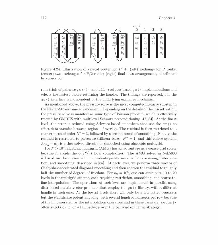
112 Chapter 4
a0a1a3a3
�
�
�
�
�
b0b1b2b3
�
�
�
�
�
c0c1
�
�
�
�
�d1d2d3
�
�
�
�
�a0c0a1c1
�
�
�
�
�
b0b1d1
�
�
�
�
�a3a3
�
�
�
�
�
d2b2d3b3
�
�
�
�
�a0c0b0
0rank
b1d1a1c1
1
d2b2
2
d3b3a3a3
3
Figure 4.24: Illustration of crystal router for P=4: (left) exchange for P ranks;(center) two exchanges for P/2 ranks; (right) final data arrangement, distributedby subscript.
runs trials of pairwise-, cr()-, and all_reduce-based gs() implementations and
selects the fastest before returning the handle. The timings are reported, but the
gs() interface is independent of the underlying exchange mechanism.
As mentioned above, the pressure solve is the most compute-intensive substep in
the Navier-Stokes time advancement. Depending on the details of the discretization,
the pressure solve is manifest as some type of Poisson problem, which is effectively
treated by GMRES with multilevel Schwarz preconditioning [47, 84]. At the finest
level, the error is reduced using Schwarz-based smoothers that use the cr() to
effect data transfer between regions of overlap. The residual is then restricted to a
coarser mesh of order N ′ = 3, followed by a second round of smoothing. Finally, the
residual is restricted to piecewise trilinear bases, N ′′ = 1, and this coarse system,
A0p0 = g0, is either solved directly or smoothed using algebraic multigrid.
For P > 104, algebraic multigrid (AMG) has an advantage as a coarse-grid solver
because it avoids the O(P 2/3) local complexities. The AMG solver in Nek5000
is based on the optimized independent-quality metrics for coarsening, interpola-
tion, and smoothing, described in [85]. At each level, we perform three sweeps of
Chebyshev-accelerated diagonal smoothing and then coarsen the residual to roughly
half the number of degrees of freedom. For n0 = 106, one can anticipate 10 to 20
levels in the multigrid scheme, each requiring restriction, smoothing, and coarse-to-
fine interpolation. The operations at each level are implemented in parallel using
distributed matrix-vector products that employ the gs() library, with a different
handle in each case. At the lowest levels there will only be a few active processes
but the stencils are potentially long, with several hundred nonzeros per row because
of the fill generated by the interpolation operators and in these cases gs_setup()often selects cr() or all_reduce over the pairwise exchange strategy.

5 Fun with Datatypes
This chapter discusses some of the more advanced features from the MPI stan-
dard that have not arisen in the discussion so far, particularly in the area of MPI
datatypes. The chapter also provides a more complete discussion of some features
already introduced briefly. We use the opportunity to introduce several interesting
example programs.
5.1 MPI Datatypes
One of MPI’s unusual features is the introduction of a datatype argument for all
messages sent and received. In the early chapters of this book, we relied primarily
on elementary datatypes that correspond to the base datatypes in the host program-
ming language—integers, floating-point numbers, and so forth, and arrays of these.
In this section we discuss the complete set of datatypes and take the opportunity
to describe the full power of MPI’s derived datatype features.
5.1.1 Basic Datatypes and Concepts
MPI provides a rich set of predefined datatypes. These include all of the basic
datatypes in C (Table 5.1) and Fortran (Table 5.2). Included in both lists are
two datatypes specific to MPI: MPI_BYTE and MPI_PACKED. MPI_BYTE refers to
a byte that is defined as eight binary digits. Many C and Fortran programmers
may wonder why this is needed when they have MPI_CHAR and MPI_CHARACTER,respectively. There are two reasons. First, while many implementations represent
char and character as bytes, this representation is not required. A version of
C for Japanese could choose 16-bit chars, for example. The second reason is that
in a heterogeneous environment, machines may have different character sets. For
example, a system that uses ASCII uses different bits to represent the character Athan does a system that uses EBCDIC. MPI_PACKED is described in Section 5.2.3.
Tables 5.1 and 5.2 do not include the MPI datatypes that correspond to language
datatypes that are not part of the language standard but are common extensions.
Vendor-specific implementations of Fortran, in particular, often have additional
datatypes. In Fortran 77, for example, the most common was DOUBLE COMPLEX,the double precision counterpart to COMPLEX, which is not, in fact, part of Fortran
77. The MPI standard could hardly mandate datatypes not part of the language
standards, and so such datatypes are not a required part of an MPI implemen-
tation. However, many Fortran implementations do support DOUBLE COMPLEX,along with types such as REAL*8 (8-byte reals) and INTEGER*2 (2-byte integers).
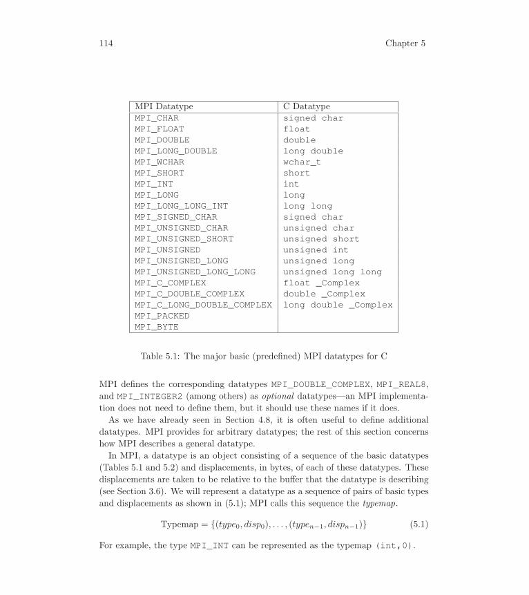
114 Chapter 5
MPI Datatype C DatatypeMPI_CHAR signed charMPI_FLOAT floatMPI_DOUBLE doubleMPI_LONG_DOUBLE long doubleMPI_WCHAR wchar_tMPI_SHORT shortMPI_INT intMPI_LONG longMPI_LONG_LONG_INT long longMPI_SIGNED_CHAR signed charMPI_UNSIGNED_CHAR unsigned charMPI_UNSIGNED_SHORT unsigned shortMPI_UNSIGNED unsigned intMPI_UNSIGNED_LONG unsigned longMPI_UNSIGNED_LONG_LONG unsigned long longMPI_C_COMPLEX float _ComplexMPI_C_DOUBLE_COMPLEX double _ComplexMPI_C_LONG_DOUBLE_COMPLEX long double _ComplexMPI_PACKEDMPI_BYTE
Table 5.1: The major basic (predefined) MPI datatypes for C
MPI defines the corresponding datatypes MPI_DOUBLE_COMPLEX, MPI_REAL8,and MPI_INTEGER2 (among others) as optional datatypes—an MPI implementa-
tion does not need to define them, but it should use these names if it does.
As we have already seen in Section 4.8, it is often useful to define additional
datatypes. MPI provides for arbitrary datatypes; the rest of this section concerns
how MPI describes a general datatype.
In MPI, a datatype is an object consisting of a sequence of the basic datatypes
(Tables 5.1 and 5.2) and displacements, in bytes, of each of these datatypes. These
displacements are taken to be relative to the buffer that the datatype is describing
(see Section 3.6). We will represent a datatype as a sequence of pairs of basic types
and displacements as shown in (5.1); MPI calls this sequence the typemap.
Typemap = {(type0, disp0), . . . , (typen−1, dispn−1)} (5.1)
For example, the type MPI_INT can be represented as the typemap (int,0).
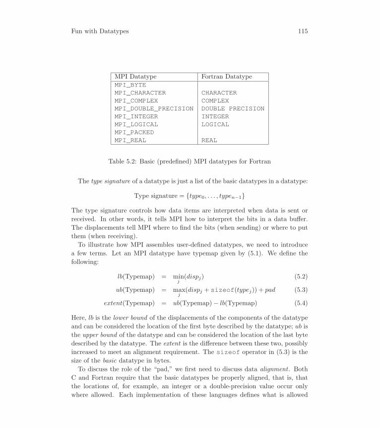
Fun with Datatypes 115
MPI Datatype Fortran DatatypeMPI_BYTEMPI_CHARACTER CHARACTERMPI_COMPLEX COMPLEXMPI_DOUBLE_PRECISION DOUBLE PRECISIONMPI_INTEGER INTEGERMPI_LOGICAL LOGICALMPI_PACKEDMPI_REAL REAL
Table 5.2: Basic (predefined) MPI datatypes for Fortran
The type signature of a datatype is just a list of the basic datatypes in a datatype:
Type signature = {type0, . . . , typen−1}
The type signature controls how data items are interpreted when data is sent or
received. In other words, it tells MPI how to interpret the bits in a data buffer.
The displacements tell MPI where to find the bits (when sending) or where to put
them (when receiving).
To illustrate how MPI assembles user-defined datatypes, we need to introduce
a few terms. Let an MPI datatype have typemap given by (5.1). We define the
following:
lb(Typemap) = minj
(dispj) (5.2)
ub(Typemap) = maxj
(dispj + sizeof(typej)) + pad (5.3)
extent(Typemap) = ub(Typemap)− lb(Typemap) (5.4)
Here, lb is the lower bound of the displacements of the components of the datatype
and can be considered the location of the first byte described by the datatype; ub is
the upper bound of the datatype and can be considered the location of the last byte
described by the datatype. The extent is the difference between these two, possibly
increased to meet an alignment requirement. The sizeof operator in (5.3) is the
size of the basic datatype in bytes.
To discuss the role of the “pad,” we first need to discuss data alignment . Both
C and Fortran require that the basic datatypes be properly aligned, that is, that
the locations of, for example, an integer or a double-precision value occur only
where allowed. Each implementation of these languages defines what is allowed

116 Chapter 5
(with some restrictions, of course). One of the most common requirements made
by an implementation of these languages is that the address of an item in bytes be a
multiple of the length of that item in bytes. For example, if an int takes four bytes,
then the address of an int must be evenly divisible by four. This requirement is
reflected in the definition of the extent of an MPI datatype. Consider the typemap
{(int, 0), (char, 4)} (5.5)
on a computer that requires that int’s be aligned on 4-byte boundaries. This
typemap has lb = min(0, 4) = 0 and ub = max(0 + 4, 4 + 1) = 5. But the next intcan only be placed with displacement eight from the int in the typemap. This
makes the extent of this typemap on the computer we are discussing eight.
To find the extent of a datatype, MPI provides the routine MPI_Type_get_-extent. The first argument is the MPI datatype; the lower bound is returned
in the second argument and the extent is returned in the third argument. In C,
the type of the second and third argument is MPI_Aint; this is an integer type
that can hold an arbitrary address. The corresponding type in Fortran is INTEGER(KIND=MPI_ADDRESS_KIND). The extents of the basic datatypes (those in Ta-
bles 5.1 and 5.2) are the same as the number of bytes in them.
The size of a datatype is the number of bytes that the data takes up. This is given
by MPI_Type_size; the first argument is the datatype, and the size is returned
in the second argument. The difference between the extent and size of a datatype
is illustrated by the typemap in (5.5): the size is five bytes, but the extent (on a
computer that requires ints be aligned on four-byte boundaries) is eight bytes.
Bindings for the datatype routines described here are given in Tables 5.3 and 5.4.
While an int was large enough to hold the size of an MPI datatype when MPI
was defined, many systems now have more than 2 gigabytes of memory, which is
the greatest number of bytes that can be described by a signed 32-bit integer. Since
many systems today use what is sometimes calls the “LP64” model, where longand pointers (e.g., void *) are 64-bit and int are 32-bits, the output value from
MPI_Type_size may not fit in an int or Fortran INTEGER. MPI-3 has added
special routines for the rare cases where an MPI datatype is too large for an int;these are discussed in Using Advanced MPI [55], Chapter 8.
5.1.2 Derived Datatypes
The typemap is a completely general way of describing an arbitrary datatype.
However, it may not be convenient, particularly if the resulting typemap contains
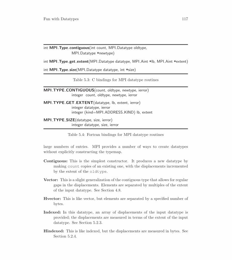
Fun with Datatypes 117
int MPI Type contiguous(int count, MPI Datatype oldtype,
MPI Datatype *newtype)
int MPI Type get extent(MPI Datatype datatype, MPI Aint *lb, MPI Aint *extent)
int MPI Type size(MPI Datatype datatype, int *size)
Table 5.3: C bindings for MPI datatype routines
MPI TYPE CONTIGUOUS(count, oldtype, newtype, ierror)integer count, oldtype, newtype, ierror
MPI TYPE GET EXTENT(datatype, lb, extent, ierror)integer datatype, ierrorinteger (kind=MPI ADDRESS KIND) lb, extent
MPI TYPE SIZE(datatype, size, ierror)integer datatype, size, ierror
Table 5.4: Fortran bindings for MPI datatype routines
large numbers of entries. MPI provides a number of ways to create datatypes
without explicitly constructing the typemap.
Contiguous: This is the simplest constructor. It produces a new datatype by
making count copies of an existing one, with the displacements incremented
by the extent of the oldtype.
Vector: This is a slight generalization of the contiguous type that allows for regular
gaps in the displacements. Elements are separated by multiples of the extent
of the input datatype. See Section 4.8.
Hvector: This is like vector, but elements are separated by a specified number of
bytes.
Indexed: In this datatype, an array of displacements of the input datatype is
provided; the displacements are measured in terms of the extent of the input
datatype. See Section 5.2.3.
Hindexed: This is like indexed, but the displacements are measured in bytes. See
Section 5.2.4.
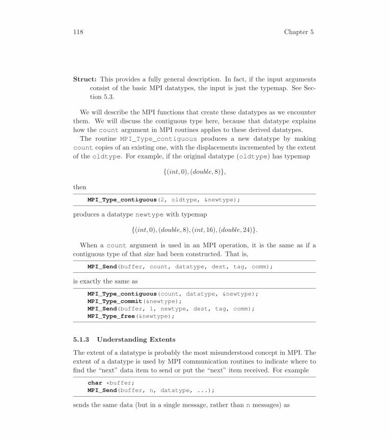
118 Chapter 5
Struct: This provides a fully general description. In fact, if the input arguments
consist of the basic MPI datatypes, the input is just the typemap. See Sec-
tion 5.3.
We will describe the MPI functions that create these datatypes as we encounter
them. We will discuss the contiguous type here, because that datatype explains
how the count argument in MPI routines applies to these derived datatypes.
The routine MPI_Type_contiguous produces a new datatype by making
count copies of an existing one, with the displacements incremented by the extent
of the oldtype. For example, if the original datatype (oldtype) has typemap
{(int, 0), (double, 8)},
then
MPI_Type_contiguous(2, oldtype, &newtype);
produces a datatype newtype with typemap
{(int, 0), (double, 8), (int, 16), (double, 24)}.
When a count argument is used in an MPI operation, it is the same as if a
contiguous type of that size had been constructed. That is,
MPI_Send(buffer, count, datatype, dest, tag, comm);
is exactly the same as
MPI_Type_contiguous(count, datatype, &newtype);MPI_Type_commit(&newtype);MPI_Send(buffer, 1, newtype, dest, tag, comm);MPI_Type_free(&newtype);
5.1.3 Understanding Extents
The extent of a datatype is probably the most misunderstood concept in MPI. The
extent of a datatype is used by MPI communication routines to indicate where to
find the “next” data item to send or put the “next” item received. For example
char *buffer;MPI_Send(buffer, n, datatype, ...);
sends the same data (but in a single message, rather than n messages) as

Fun with Datatypes 119
char *buffer;MPI_Type_get_extent(datatype, &lb, &extent);for (i=0; i<n; i++) {
MPI_Send(buffer + (i * extent), 1, datatype, ...);}
To simplify this example, we have declared buffer as type char and assumed
that sizeof(char) is one byte.
We can see from this that the extent of a datatype is not its size; it is closest
to being the stride of a datatype: the distance (in bytes) to skip (stride) from the
start of one instance of the datatype to the start of another instance of a datatype.
We will come back to this topic in Section 5.4, where we will see how to use the
extent to send data separated by regular gaps.
5.2 The N-Body Problem
Many simulations involve computing the interaction of a large number of particles
or objects. If the force between the particles is completely described by adding the
forces between all pairs of particles and if the force between each pair acts along
the line between them, this is called an N-body central force problem (often just an
N-body problem). Such a problem is a good choice for parallelization because it can
be described with N items (the particles) but requires O(N2) computation (all the
pairs of particles). Thus, we can expect good speedups for large problems because
the communication between processes will be small relative to the computation.1
In this section, we will use the N-body problem to describe a number of MPI
features, including new collective operations, persistent communication requests,
and new derived datatypes.
In implementing an N-body code, we need first to decide how the particles are
distributed among the processes. One simple way is to divide the particles evenly
among the processes. For example, if there are 1000 particles and 10 processes, we
put the first 100 particles on process 0, the second 100 particles on process 1, and
so forth. To compute the forces on the particles, each process must access all the
particles on the other processes. (An important optimization involves exploiting
the fact that the forces are equal and opposite; this can reduce the computation by
a factor of 2. For simplicity, we do not make use of this property.)
1As we’ll note in Section 5.2.3, despite this obvious calculation of the work involved, somealgorithms can approximate the solution to high accuracy with fewer computations.

120 Chapter 5
To begin, we define a particle datatype. Let us assume that a particle is defined
by the structure
typedef struct {double x, y, z;double mass;
} Particle;
and that the particles are stored in an array:
Particle particles[MAX_PARTICLES];
To send this data, we could just send four doubles for each particle, but it makes
more sense in MPI to create a datatype for a particle consisting of four doubles:
MPI_Type_contiguous(4, MPI_DOUBLE, &particletype);MPI_Type_commit(&particletype);
We should use MPI_Type_indexed or more generally MPI_Type_create_-struct to build this structure, but MPI_Type_contiguous will work on almost
any system for this particular case. We will cover the use of MPI_Type_create_-struct in Section 5.3.
5.2.1 Gather
The simplest approach is for all processes to exchange all the particles and then
compute with them. In this approach, all processes will have copies of all of the
particles, computing only the forces on the particles held locally.2 For example,
each process could do
Particle *(particleloc[]);...MPI_Comm_size(MPI_COMM_WORLD, &size);for (i=0; i<size; i++)
MPI_Send(particles, count, particletype, i, 0,MPI_COMM_WORLD);
for (i=0; i<size; i++) {MPI_Recv(particleloc[i], MAX_PARTICLES, particletype, i, 0,
MPI_COMM_WORLD, &status);/* Use status to determine how many particles were sent */MPI_Get_count(&status, particletype, &mycount);
}
2This approach is suitable only for relatively small number of particles; it may be used if theforces are particularly complicated or if long spans of time need to be computed.

Fun with Datatypes 121
(For reasons that will soon be clear, we have deliberately left out the sends and
receives from a process to itself in this code.) This code has many problems: it does
not scale (it takes time proportional to the number of processes), it may deadlock
(because the code requires that MPI_Send provide buffering), and it needs the
locations particleloc[i] computed before the code can be used. We could use
the techniques in Chapter 4 to get around the deadlock (buffering) problem, but the
other problems require more care. Fortunately, MPI provides routines to handle
this common case. We will show how the routines MPI_Allgather and MPI_-Allgatherv can be used to provide efficient ways to communicate data between
processes.
First, let us handle the problem of determining how many particles each process
has. Let each process have count contain the number of particles that it holds.
We wish to fill an array counts such that counts[i] contains the number of
particles on the ith process. One way to do this is to gather all the data to a single
process and then use MPI_Bcast to send the data to all the processes. The routine
that accomplishes this is MPI_Gather.
int count, counts[];...root = 0;MPI_Gather(&count, 1, MPI_INT, counts, 1, MPI_INT, root,
MPI_COMM_WORLD);MPI_Comm_size(MPI_COMM_WORLD, &size);MPI_Bcast(counts, size, MPI_INT, root, MPI_COMM_WORLD);
The gather operation takes the data being sent by the ith process and places
it in the ith location in the receive buffer on the root process. Only the process
designated as the root receives the data.
Tables 5.5 and 5.6 show the bindings for the gather operations. The first three
arguments describe the data to be sent; the fourth through sixth arguments describe
the data to be received. For MPI_Gather, the seventh argument indicates which
process will receive the data. MPI_Gather requires that all processes, including the
root, send the same amount of data and that the type signature of the sendtypematch that of the recvtype. The value of recvcount is the number of data
items sent by any one process; usually, sendtype = recvtype and sendcount= recvcount. Once all the data has been gathered to a single process, the data
can be distributed to all processes with the broadcast routine MPI_Bcast. Note
also that the recvbuf is longer than the sendbuf except for the trivial case where
the sendcount is zero.

122 Chapter 5
P0
P1
P2
P3
A
B
C
D
B C D
Figure 5.1: Data motion for a gather operation with p0 as root
Just as with MPI_Reduce and MPI_Allreduce, it can be more convenient and
efficient to combine the gather and broadcast operations into a single operation.
MPI_Allgather does this; the code for collecting the counts onto all processes is
shown here:
int counts[MAX_PROCESSES];MPI_Allgather(&count, 1, MPI_INT, counts, 1, MPI_INT,
MPI_COMM_WORLD);
Note that the recvcount argument is a scalar; it indicates the number of items
received from each process, not the sum of the number of items received from all
processes.
If all processes had the same number of particles, then we could use MPI_-Allgather to get the particles:
MPI_Allgather(myparticles, count, particletype,allparticles, count, particletype, MPI_COMM_WORLD);
In most cases, however, each process will have different numbers of particles. In this
case, we can use a variant of MPI_Allgather that permits differing sizes of data
to be sent from each process. The routine MPI_Allgatherv takes the lengths of
each item to be received and the displacement relative to the receive buffer (in units
of the extent of the receive datatype) where the item will be stored. That is, on
the ith process, recvcount[i] items are received into the receive buffer starting

Fun with Datatypes 123
int MPI Gather(const void *sendbuf, int sendcount, MPI Datatype sendtype,
void *recvbuf, int recvcount, MPI Datatype recvtype, int root,MPI Comm comm)
int MPI Allgather(const void *sendbuf, int sendcount, MPI Datatype sendtype,
void *recvbuf, int recvcount, MPI Datatype recvtype,MPI Comm comm)
int MPI Allgatherv(const void *sendbuf, int sendcount, MPI Datatype sendtype,
void *recvbuf, const int *recvcounts, const int *displs,MPI Datatype recvtype, MPI Comm comm)
Table 5.5: C bindings for N-body code
MPI GATHER(sendbuf, sendcount, sendtype, recvbuf, recvcount, recvtype, root,comm, ierror)
<type> sendbuf(*), recvbuf(*)integer sendcount, sendtype, recvcount, recvtype, root, comm, ierror
MPI ALLGATHER(sendbuf, sendcount, sendtype, recvbuf, recvcount, recvtype,comm, ierror)
<type> sendbuf(*), recvbuf(*)integer sendcount, sendtype, recvcount, recvtype, comm, ierror
MPI ALLGATHERV(sendbuf, sendcount, sendtype, recvbuf, recvcounts, rdispls,recvtype, comm, ierror)
<type> sendbuf(*), recvbuf(*)
integer sendcount, sendtype,recvcounts(*), displs(*), recvtype,comm, ierror
Table 5.6: Fortran bindings for N-body code

124 Chapter 5
at location recvbuf + displs[i] (the value of displs[i] is relative to the
datatype of the receive buffer). In our case, we wish to receive the particles into
a single array allparticles. The displacement for the ith process is simply the
sum of counts for processes 0 through i− 1. The code to gather all of the particles
is
displacements[0] = 0;for (i=1; i<size; i++)
displacements[i] = counts[i-1] + displacements[i-1];MPI_Allgatherv(myparticles, count, particletype,
allparticles, counts, displacements, particletype,MPI_COMM_WORLD);
In case you are wondering what MPI_Gather and MPI_Allgather have sep-
arate datatype arguments for the send and receive buffers, the reason is that MPI
requires only that the type signatures match. For example, by using a different MPI
datatype for the send and receive types, the data can be transposed “on the fly”.
To do this, the send type could specify a row of a matrix (stored in column-major,
with n columns, and created with MPI_Type_vector) with a sendcount of 1and the receive type could specify contiguous doubles with a receive count of n and
receive type of MPI_DOUBLE.
5.2.2 Nonblocking Pipeline
In this section we present another approach to the communications in the N-body
problem. When using MPI Allgatherv, the computation and communication
phases are distinct and nonoverlapping. A different approach is to use nonblocking
communications, overlapping the communication with the computation. There are
a number of ways to do this. One of the simplest is to create a pipeline where each
process receives some data from the left and sends data to the right. While the
data is arriving, computations on data previously received are carried out. This
approach is shown below:
while (not done) {MPI_Irecv(buf1, ..., source=left, ..., &handles[0]);MPI_Isend(buf2, ..., dest=right, ..., &handles[1]);<compute with buf2>MPI_Waitall(2, handles, statuses);<swap buf1 and buf2>
}

Fun with Datatypes 125
If enough data is being sent and the MPI implementation and computer hardware
can effectively overlap computation and communication, this approach can be faster
than using MPI_Allgatherv.In many simulations, thousands to millions of these steps may be taken. As
written above, each step requires the creation of a send and a receive request, with
the same parameters being used in each cycle. In this situation, it is possible for
a sophisticated MPI implementation to take advantage of the fact that the same
operation is being performed many times. To express this, MPI provides routines
to create “persistent” send and receive objects that can be used to perform the
same operation multiple times. The form of the create call is very similar to a
nonblocking send and receive; the only difference is that no communication takes
place. Just as for the nonblocking operations MPI_Isend and MPI_Irecv, theseroutines return an MPI_Request. In order to begin communication with the
request, the routine MPI_Start must first be called with the request. In order to
complete the communication, one of the wait routines, such as MPI_Wait, must
be called. Once a wait has succeeded with the request, MPI_Start may be called
again. Multiple persistent communications may be initiated with MPI_Startall.The code
MPI_Irecv(..., &request);
is equivalent to
MPI_Recv_init(..., &request);MPI_Start(&request);
An MPI_Wait on an MPI_Irecv request is equivalent to
MPI_Wait(&request, &status);MPI_Request_free(&request);
In the N-body problem, the code is complicated by the fact that, if all processes
do not have the same number of particles, then there must be a different MPI_-Request created for each number of particles (or, for simplicity, for each process).
The code is shown in Figure 5.2.3
Note that we call the communication routines only size-1 times; we do not
need to send the particles back to their original processes. A complete N-body
code using this approach is available in ‘advmsg/nbodypipe.c’. Bindings for
the MPI routines used here are shown in Tables 5.7 and 5.8.
3For Fortran programmers, the C expression a % b is roughly equivalent to the Fortran ex-pression mod(a,b).
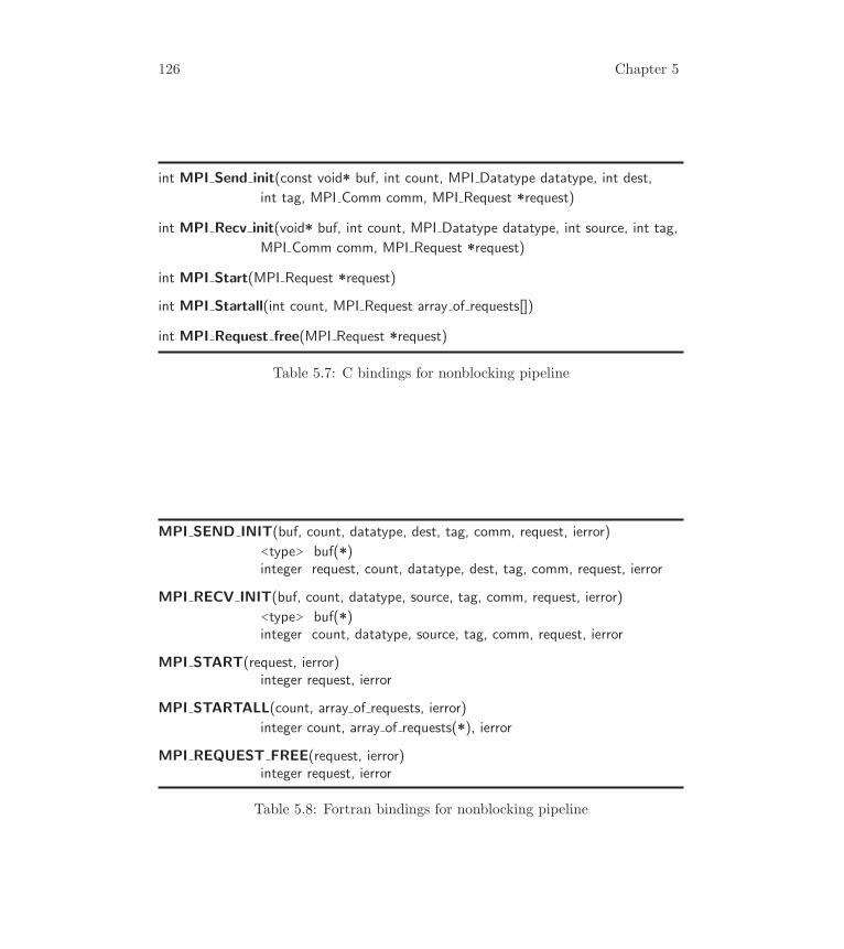
126 Chapter 5
int MPI Send init(const void* buf, int count, MPI Datatype datatype, int dest,
int tag, MPI Comm comm, MPI Request *request)
int MPI Recv init(void* buf, int count, MPI Datatype datatype, int source, int tag,
MPI Comm comm, MPI Request *request)
int MPI Start(MPI Request *request)
int MPI Startall(int count, MPI Request array of requests[])
int MPI Request free(MPI Request *request)
Table 5.7: C bindings for nonblocking pipeline
MPI SEND INIT(buf, count, datatype, dest, tag, comm, request, ierror)
<type> buf(*)integer request, count, datatype, dest, tag, comm, request, ierror
MPI RECV INIT(buf, count, datatype, source, tag, comm, request, ierror)
<type> buf(*)integer count, datatype, source, tag, comm, request, ierror
MPI START(request, ierror)integer request, ierror
MPI STARTALL(count, array of requests, ierror)
integer count, array of requests(*), ierror
MPI REQUEST FREE(request, ierror)integer request, ierror
Table 5.8: Fortran bindings for nonblocking pipeline
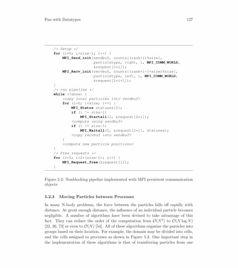
Fun with Datatypes 127
/* Setup */for (i=0; i<size-1; i++) {
MPI_Send_init(sendbuf, counts[(rank+i)%size],particletype, right, i, MPI_COMM_WORLD,&request[2*i]);
MPI_Recv_init(recvbuf, counts[(rank+i-1+size)%size],particletype, left, i, MPI_COMM_WORLD,&request[2*i+1]);
}/* run pipeline */while (!done) {
<copy local particles into sendbuf>for (i=0; i<size; i++) {
MPI_Status statuses[2];if (i != size-1)
MPI_Startall(2, &request[2*i]);<compute using sendbuf>if (i != size-1)
MPI_Waitall(2, &request[2*i], statuses);<copy recvbuf into sendbuf>
}<compute new particle positions>
}/* Free requests */for (i=0; i<2*(size-1); i++) {
MPI_Request_free(&request[i]);}
Figure 5.2: Nonblocking pipeline implemented with MPI persistent communicationobjects
5.2.3 Moving Particles between Processes
In many N-body problems, the force between the particles falls off rapidly with
distance. At great enough distance, the influence of an individual particle becomes
negligible. A number of algorithms have been devised to take advantage of this
fact. They can reduce the order of the computation from O(N2) to O(N logN)
[22, 26, 73] or even to O(N) [54]. All of these algorithms organize the particles into
groups based on their location. For example, the domain may be divided into cells,
and the cells assigned to processes as shown in Figure 5.3. One important step in
the implementation of these algorithms is that of transferring particles from one
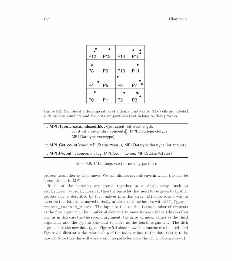
128 Chapter 5
P0 P1 P2 P3
P4 P5 P6 P7
P9 P10 P11
P12 P13 P14 P15
P8
Figure 5.3: Sample of a decomposition of a domain into cells. The cells are labeledwith process numbers and the dots are particles that belong to that process.
int MPI Type create indexed block(int count, int blocklength,const int array of displacements[], MPI Datatype oldtype,
MPI Datatype *newtype)
int MPI Get count(const MPI Status *status, MPI Datatype datatype, int *count)
int MPI Probe(int source, int tag, MPI Comm comm, MPI Status *status)
Table 5.9: C bindings used in moving particles
process to another as they move. We will discuss several ways in which this can be
accomplished in MPI.
If all of the particles are stored together in a single array, such as
Particles myparticles[], then the particles that need to be given to another
process can be described by their indices into this array. MPI provides a way to
describe the data to be moved directly in terms of these indices with MPI_Type_-create_indexed_block. The input to this routine is the number of elements
as the first argument, the number of elements to move for each index (this is often
one, as in this case) as the second argument, the array of index values as the third
argument, and the type of the data to move as the fourth argument. The fifth
argument is the new data type. Figure 5.4 shows how this routine can be used, and
Figure 5.5 illustrates the relationship of the index values to the data that is to be
moved. Note that this will work even if no particles leave the cell (n_to_move=0).

Fun with Datatypes 129
MPI TYPE CREATE INDEXED BLOCK(count, blocklength,array of displacements, oldtype, newtype, ierror)
integer count, blocklength, array of displacement(*), oldtype,newtype, ierror
MPI GET COUNT(status, datatype, count, ierror)
integer status(*), datatype, count, ierror
MPI PROBE(source, tag, comm, status, ierror)integer source, tag, comm, status(MPI STATUS SIZE), ierror
Table 5.10: Fortran bindings used in moving particles
n_to_move = 0;for (i=0; i<count; i++) {
if (...particle exited cell...) {elmoffset[n_to_move] = i;n_to_move++;
}}MPI_Type_create_indexed_block(n_to_move, 1, elmoffset,
particletype, &sendtype);MPI_Type_commit(&sendtype);MPI_Send(myparticles, 1, sendtype, dest, tag, comm);MPI_Type_free(&sendtype);
Figure 5.4: Sketch of code to move particles from one process to another
myparticles
9 27 39 142
9 27 39 142elmoffset
Only these particles need to be sent
0
Figure 5.5: Illustration of the array_of_displacements argument in Figure 5.4
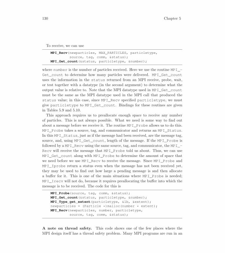
130 Chapter 5
To receive, we can use
MPI_Recv(newparticles, MAX_PARTICLES, particletype,source, tag, comm, &status);
MPI_Get_count(&status, particletype, &number);
where number is the number of particles received. Here we use the routine MPI_-Get_count to determine how many particles were delivered. MPI_Get_countuses the information in the status returned from an MPI receive, probe, wait,
or test together with a datatype (in the second argument) to determine what the
output value is relative to. Note that the MPI datatype used in MPI_Get_countmust be the same as the MPI datatype used in the MPI call that produced the
status value; in this case, since MPI_Recv specified particletype, we must
give particletype to MPI_Get_count. Bindings for these routines are given
in Tables 5.9 and 5.10.
This approach requires us to preallocate enough space to receive any number
of particles. This is not always possible. What we need is some way to find out
about a message before we receive it. The routine MPI_Probe allows us to do this.
MPI_Probe takes a source, tag, and communicator and returns an MPI_Status.In this MPI_Status, just as if the message had been received, are the message tag,
source, and, using MPI_Get_count, length of the message. If the MPI_Probe is
followed by a MPI_Recv using the same source, tag, and communicator, the MPI_-Recv will receive the message that MPI_Probe told us about. Thus, we can use
MPI_Get_count along with MPI_Probe to determine the amount of space that
we need before we use MPI_Recv to receive the message. Since MPI_Probe and
MPI_Iprobe return a status even when the message has not been received yet,
they may be used to find out how large a pending message is and then allocate
a buffer for it. This is one of the main situations where MPI_Probe is needed;
MPI_Irecv will not do, because it requires preallocating the buffer into which the
message is to be received. The code for this is
MPI_Probe(source, tag, comm, &status);MPI_Get_count(&status, particletype, &number);MPI_Type_get_extent(particletype, &lb, &extent);newparticles = (Particle *)malloc(number * extent);MPI_Recv(newparticles, number, particletype,
source, tag, comm, &status);
A note on thread safety. This code shows one of the few places where the
MPI design itself has a thread safety problem. Many MPI programs are run in an
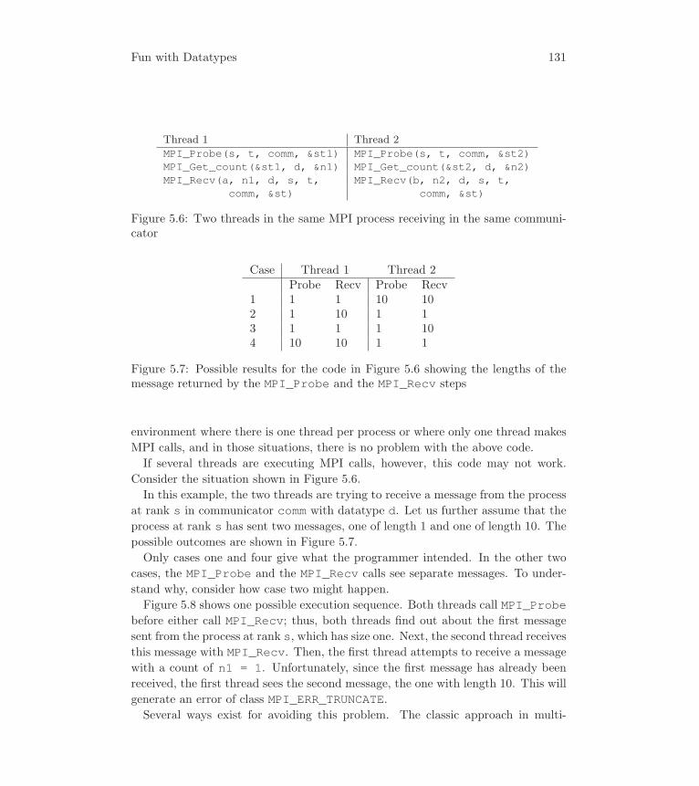
Fun with Datatypes 131
Thread 1 Thread 2
MPI_Probe(s, t, comm, &st1) MPI_Probe(s, t, comm, &st2)MPI_Get_count(&st1, d, &n1) MPI_Get_count(&st2, d, &n2)MPI_Recv(a, n1, d, s, t, MPI_Recv(b, n2, d, s, t,
comm, &st) comm, &st)
Figure 5.6: Two threads in the same MPI process receiving in the same communi-cator
Case Thread 1 Thread 2Probe Recv Probe Recv
1 1 1 10 102 1 10 1 13 1 1 1 104 10 10 1 1
Figure 5.7: Possible results for the code in Figure 5.6 showing the lengths of themessage returned by the MPI_Probe and the MPI_Recv steps
environment where there is one thread per process or where only one thread makes
MPI calls, and in those situations, there is no problem with the above code.
If several threads are executing MPI calls, however, this code may not work.
Consider the situation shown in Figure 5.6.
In this example, the two threads are trying to receive a message from the process
at rank s in communicator comm with datatype d. Let us further assume that the
process at rank s has sent two messages, one of length 1 and one of length 10. The
possible outcomes are shown in Figure 5.7.
Only cases one and four give what the programmer intended. In the other two
cases, the MPI_Probe and the MPI_Recv calls see separate messages. To under-
stand why, consider how case two might happen.
Figure 5.8 shows one possible execution sequence. Both threads call MPI_Probebefore either call MPI_Recv; thus, both threads find out about the first message
sent from the process at rank s, which has size one. Next, the second thread receives
this message with MPI_Recv. Then, the first thread attempts to receive a message
with a count of n1 = 1. Unfortunately, since the first message has already been
received, the first thread sees the second message, the one with length 10. This will
generate an error of class MPI_ERR_TRUNCATE.Several ways exist for avoiding this problem. The classic approach in multi-
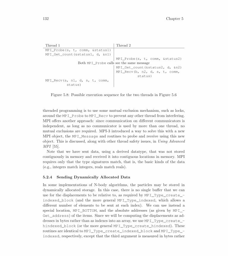
132 Chapter 5
Thread 1 Thread 2
MPI_Probe(s, t, comm, &status1)MPI_Get_count(&status1, d, &n1)
MPI_Probe(s, t, comm, &status2)Both MPI_Probe calls see the same message
MPI_Get_count(&status2, d, &n2)MPI_Recv(b, n2, d, s, t, comm,
status)MPI_Recv(a, n1, d, s, t, comm,
status)
Figure 5.8: Possible execution sequence for the two threads in Figure 5.6
threaded programming is to use some mutual exclusion mechanism, such as locks,
around the MPI_Probe to MPI_Recv to prevent any other thread from interfering.
MPI offers another approach: since communication on different communicators is
independent, as long as no communicator is used by more than one thread, no
mutual exclusions are required. MPI-3 introduced a way to solve this with a new
MPI object, the MPI_Message and routines to probe and receive using this new
object. This is discussed, along with other thread safety issues, in Using Advanced
MPI [55].
Note that we have sent data, using a derived datatype, that was not stored
contiguously in memory and received it into contiguous locations in memory. MPI
requires only that the type signatures match, that is, the basic kinds of the data
(e.g., integers match integers, reals match reals).
5.2.4 Sending Dynamically Allocated Data
In some implementations of N-body algorithms, the particles may be stored in
dynamically allocated storage. In this case, there is no single buffer that we can
use for the displacements to be relative to, as required by MPI_Type_create_-indexed_block (and the more general MPI_Type_indexed, which allows a
different number of elements to be sent at each index). We can use instead a
special location, MPI_BOTTOM, and the absolute addresses (as given by MPI_-Get_address) of the items. Since we will be computing the displacements as ad-
dresses in bytes rather than as indexes into an array, we use MPI_Type_create_-hindexed_block (or the more general MPI_Type_create_hindexed). Theseroutines are identical to MPI_Type_create_indexed_block and MPI_Type_-indexed, respectively, except that the third argument is measured in bytes rather

Fun with Datatypes 133
MPI_Aint elmoffset[MAX_PARTICLES];n_to_move = 0;while (particle) {
if (particle exited cell) {MPI_Get_address(particle, &elmoffset[n_to_move]);n_to_move++;<make sure to unlink particle and de-allocate>
}else {
particle = particle->next;}
}MPI_Type_create_hindexed_block(n_to_move, 1, elmoffset,
particletype, &particlemsg);MPI_Type_commit(&particlemsg);MPI_Send(MPI_BOTTOM, 1, particlemsg, dest, tag, comm);MPI_Type_free(&particlemsg);
Figure 5.9: Sketch of code to move dynamically allocated particles to other pro-cesses
than in elements. For example, if the particles are stored in a linked list whose
elements are dynamically created, we can use the code in Figure 5.9.
The routine MPI_Get_address takes an item as the first argument and returns
its address, with type (in C) of MPI_Aint as the second argument. Fortran pro-
grammers will appreciate this function, but C programmers may be a bit puzzled by
its use, particularly in a C program. The reason is that in many C implementations,
the value of a pointer (as an integer) is implemented as the address in memory of
the item pointed at. This is not required in C, however, and on many important
machines (for example, supercomputers with word, not byte, addressability and
practically every personal computer on the planet in the 1990s) pointers were not
addresses. While at this writing the use of an address as the pointer is nearly
universal, the growth in the use of accelerators, such as GPGPUs with their own
memory space, has led some researchers to consider exploiting this feature of C and
once again using part of the pointer to describe different kinds of address spaces.
Using MPI_Get_address in C programs helps maintain portability. Bindings for
these routines are shown in Tables 5.11 and 5.12.
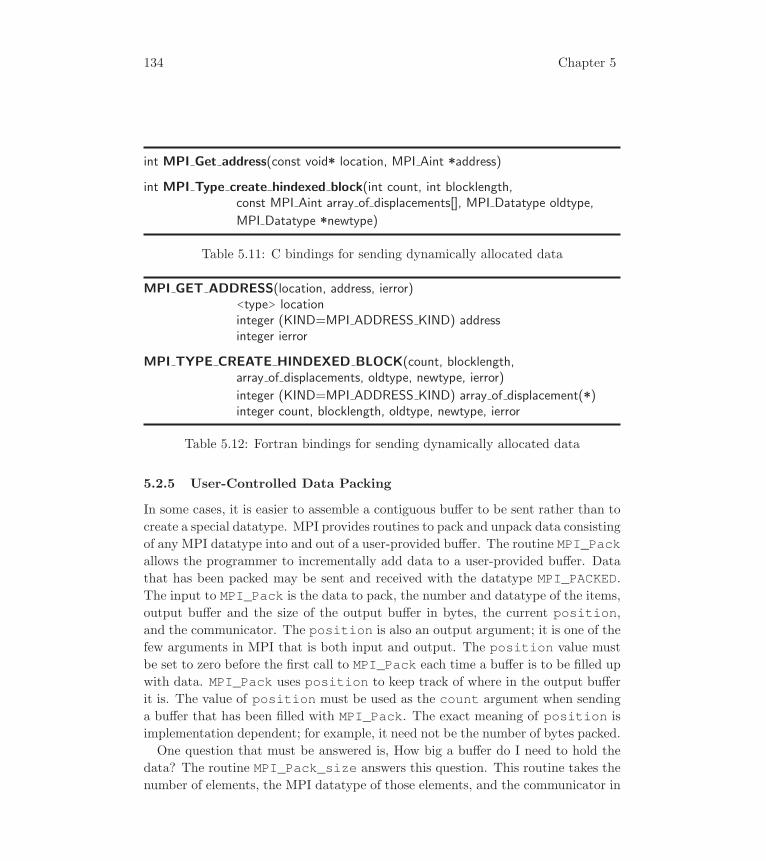
134 Chapter 5
int MPI Get address(const void* location, MPI Aint *address)
int MPI Type create hindexed block(int count, int blocklength,const MPI Aint array of displacements[], MPI Datatype oldtype,
MPI Datatype *newtype)
Table 5.11: C bindings for sending dynamically allocated data
MPI GET ADDRESS(location, address, ierror)<type> locationinteger (KIND=MPI ADDRESS KIND) addressinteger ierror
MPI TYPE CREATE HINDEXED BLOCK(count, blocklength,array of displacements, oldtype, newtype, ierror)
integer (KIND=MPI ADDRESS KIND) array of displacement(*)integer count, blocklength, oldtype, newtype, ierror
Table 5.12: Fortran bindings for sending dynamically allocated data
5.2.5 User-Controlled Data Packing
In some cases, it is easier to assemble a contiguous buffer to be sent rather than to
create a special datatype. MPI provides routines to pack and unpack data consisting
of any MPI datatype into and out of a user-provided buffer. The routine MPI_Packallows the programmer to incrementally add data to a user-provided buffer. Data
that has been packed may be sent and received with the datatype MPI_PACKED.The input to MPI_Pack is the data to pack, the number and datatype of the items,
output buffer and the size of the output buffer in bytes, the current position,and the communicator. The position is also an output argument; it is one of the
few arguments in MPI that is both input and output. The position value must
be set to zero before the first call to MPI_Pack each time a buffer is to be filled up
with data. MPI_Pack uses position to keep track of where in the output buffer
it is. The value of position must be used as the count argument when sending
a buffer that has been filled with MPI_Pack. The exact meaning of position is
implementation dependent; for example, it need not be the number of bytes packed.
One question that must be answered is, How big a buffer do I need to hold the
data? The routine MPI_Pack_size answers this question. This routine takes the
number of elements, the MPI datatype of those elements, and the communicator in
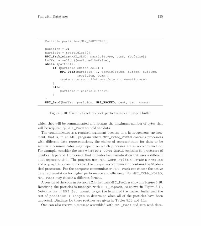
Fun with Datatypes 135
Particle particles[MAX_PARTICLES];
position = 0;particle = &particles[0];MPI_Pack_size(MAX_SEND, particletype, comm, &bufsize);buffer = malloc((unsigned)bufsize);while (particle) {
if (particle exited cell) {MPI_Pack(particle, 1, particletype, buffer, bufsize,
&position, comm);<make sure to unlink particle and de-allocate>
}else {
particle = particle->next;}
}MPI_Send(buffer, position, MPI_PACKED, dest, tag, comm);
Figure 5.10: Sketch of code to pack particles into an output buffer
which they will be communicated and returns the maximum number of bytes that
will be required by MPI_Pack to hold the data.
The communicator is a required argument because in a heterogeneous environ-
ment, that is, in an MPI program where MPI_COMM_WORLD contains processors
with different data representations, the choice of representation for data to be
sent in a communicator may depend on which processes are in a communicator.
For example, consider the case where MPI_COMM_WORLD contains 64 processors of
identical type and 1 processor that provides fast visualization but uses a different
data representation. The program uses MPI_Comm_split to create a computeand a graphics communicator; the compute communicator contains the 64 iden-
tical processors. For the compute communicator, MPI_Pack can choose the native
data representation for higher performance and efficiency. For MPI_COMM_WORLD,MPI_Pack may choose a different format.
A version of the code in Section 5.2.4 that uses MPI_Pack is shown in Figure 5.10.
Receiving the particles is managed with MPI_Unpack, as shown in Figure 5.11.
Note the use of MPI_Get_count to get the length of the packed buffer and the
test of position < length to determine when all of the particles have been
unpacked. Bindings for these routines are given in Tables 5.13 and 5.14.
One can also receive a message assembled with MPI_Pack and sent with data-
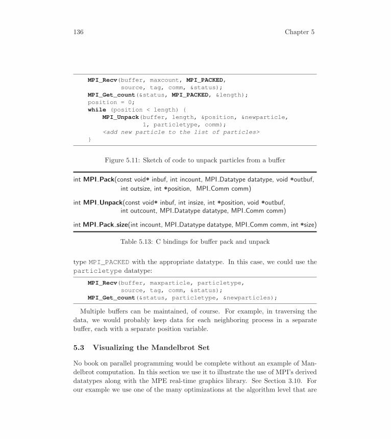
136 Chapter 5
MPI_Recv(buffer, maxcount, MPI_PACKED,source, tag, comm, &status);
MPI_Get_count(&status, MPI_PACKED, &length);position = 0;while (position < length) {
MPI_Unpack(buffer, length, &position, &newparticle,1, particletype, comm);
<add new particle to the list of particles>}
Figure 5.11: Sketch of code to unpack particles from a buffer
int MPI Pack(const void* inbuf, int incount, MPI Datatype datatype, void *outbuf,
int outsize, int *position, MPI Comm comm)
int MPI Unpack(const void* inbuf, int insize, int *position, void *outbuf,int outcount, MPI Datatype datatype, MPI Comm comm)
int MPI Pack size(int incount, MPI Datatype datatype, MPI Comm comm, int *size)
Table 5.13: C bindings for buffer pack and unpack
type MPI_PACKED with the appropriate datatype. In this case, we could use the
particletype datatype:
MPI_Recv(buffer, maxparticle, particletype,source, tag, comm, &status);
MPI_Get_count(&status, particletype, &newparticles);
Multiple buffers can be maintained, of course. For example, in traversing the
data, we would probably keep data for each neighboring process in a separate
buffer, each with a separate position variable.
5.3 Visualizing the Mandelbrot Set
No book on parallel programming would be complete without an example of Man-
delbrot computation. In this section we use it to illustrate the use of MPI’s derived
datatypes along with the MPE real-time graphics library. See Section 3.10. For
our example we use one of the many optimizations at the algorithm level that are
Fun with Datatypes 137
MPI PACK(inbuf, incount, datatype, outbuf, outcount, position, comm, ierror)
<type> inbuf(*), outbuf(*)integer incount, datatype, outcount, position, comm, ierror
MPI UNPACK(inbuf, insize, position, outbuf, outcount, datatype, comm, ierror)
<type> inbuf(*), outbuf(*)integer insize, position, outcount, datatype, comm, ierror
MPI PACK SIZE(incount, datatype, comm, size, ierror)integer incount, datatype, comm, size, ierror
Table 5.14: Fortran bindings for buffer pack and unpack
possible for programs, parallel or not, that compute graphical representations of
the Mandelbrot set.
The Mandelbrot set is a popular exercise for parallel computation because it is
so obviously a parallel application, it introduces a load-balancing problem, and the
results are fascinating to look at. To be at least a little original, we do it here with
a slightly nonstandard algorithm. We would like to think we invented this trick,
but we are not certain. Surely others have had the same idea.
Let z be a complex variable. That is, we think of z as a point (x, y) in the plane,
with multiplication on points of the plane given by
(x1, y1) · (x2, y2) = (x1x2 − y1y2, x1y2 + x2y1).
The Mandelbrot set M is defined in the following way. Given a complex number
c, consider the function fc(z) = z2 + c. Then we can compute a series of points in
the complex plane: z0 = 0, z1 = fc(0), z2 = fc(z1) = fc2(0), and so on. Either this
series remains bounded, in which case c is in M, or it gets farther and farther away
from 0, in which case it is not. It can be proven that once a point in this sequence
gets farther than a distance of 2 from the origin, the series becomes unbounded.
A “picture” of the Mandelbrot set can be made by plotting the points on the
screen. Each pixel in the display corresponds to a point c in the complex plane and
can be tested for membership in M by applying the function fc repeatedly to 0.
Either |fcn(0)| > 2 for some n, or some preset number of iterations has been reached,
in which case we give up and declare that the point c is in M and color it, say,
black. Details of the very complex boundary of M can be seen by “magnification,”
assigning the full area of the display to a small section of the complex plane. For
more on the Mandelbrot set and related topics, see [88] or [101].
138 Chapter 5
The region near the boundary ofM is interesting. Striking representations of this
area can be made by assigning a color to the pixel representing point c according
to the first value n for which |fcn(0)| > 2. As we explore the edge of M at greater
and greater magnifications, we have a sense of exploring a huge universe of great
variety. After a few random magnifications, we are likely to be looking at a part of
the plane that no one has ever looked at before.
The calculation of each pixel’s color value can be made independently of every
other pixel’s, so the program to compute such pictures is straightforwardly paral-
lelizable, just by dividing up the screen into areas, one for each process. Unfortu-
nately, this naive “prescheduled” approach works badly because of load imbalances.
Some points escape the circle of radius 2 after only a few iterations, others take
longer, and of course the points in M itself take the maximum number of itera-
tions before we give up on them. As we magnify, we need more iterations to bring
out detail, so some pixels may take thousands of times more iterations than others
before we can assign them a color.
The most natural way to overcome this load-balancing problem is with self-
scheduling. We divide up the screen into some moderately large number of squares
and devote one process (the manager) to sending them to the other processes (the
workers) for computation. Just as in the matrix-vector multiplication program in
Chapter 3, completion of a task is a request for another assignment. Some tasks
will take much longer than others (particularly the areas that are mostly black),
but unless we have very bad luck, we will be able to keep all processes busy all the
time.
We have included a parallel Mandelbrot program among the examples available
with this book. It is too long to present here, but it has three interesting aspects
that we will expand on below. Specifically, it illustrates
• the use of derived datatypes in MPI for sending scattered structures,
• an interesting technique for accelerating the computation, and
• a few more functions from the MPE graphics library.
During the initialization phase of the computation, the manager process broadcasts
a highly miscellaneous collection of data to the workers. We can think of it as
a C structure, although not all the data is stored as a single C structure. We
could broadcast each of these parameters separately, which would be wasteful of
messages (and would be expensive, because of the often high startup cost of sending
a message), or we could rearrange them into arrays of ints, arrays of doubles,

Fun with Datatypes 139
MPI TYPE CREATE HVECTOR(count, blocklength, stride, oldtype, newtype,ierror)integer (kind=MPI ADDRESS KIND) strideinteger count, blocklength, oldtype, newtype, ierror
MPI TYPE CREATE STRUCT(count, array of blocklengths,array of displacements, array of types, newtype, ierror)
integer (kind=MPI ADDRESS KIND) array of displacements(*)
integer count, array of blocklengths(*), array of types(*), newtype,ierror
Table 5.15: Fortran bindings for MPI datatype routines
int MPI Type create hvector(int count, int blocklength, MPI Aint stride,
MPI Datatype oldtype, MPI Datatype *newtype)
int MPI Type create struct(int count, const int array of blocklengths[],const MPI Aint array of displacements[],
const MPI Datatype array of types[], MPI Datatype *newtype)
Table 5.16: C bindings for MPI datatype routines
and so forth. The “MPI way” is to create a datatype that represents this structure
and send it all at once.
The algorithm we use is illustrated in Figures 5.12, 5.13, and 5.14. The example
code implements a method for accelerating the computation. The trick is based on
the fact that except at the very lowest magnification, if the border of any square
is made up of pixels all of which have the same color, then all the pixels in the
interior of the square must have that color too. This can speed things up a great
deal, especially for large areas of M itself. In order to dynamically adapt the sizes
of the squares, we do the following.
The queue of tasks to be done is managed by the manager and consists of squares
whose colors are to be computed. Initially just one task is in the queue, the entire
region selected for display. Given a square, we begin computing the colors of the
pixels on its boundary. If we get all the way around the boundary without changing
colors, then we color in the interior with the same color. If we come to a new color
while computing the boundary, then we subdivide the square into four subsquares
and send them back to the manager as new tasks, while we carry on with the
boundary. We carefully keep the squares nested tightly so that we never compute
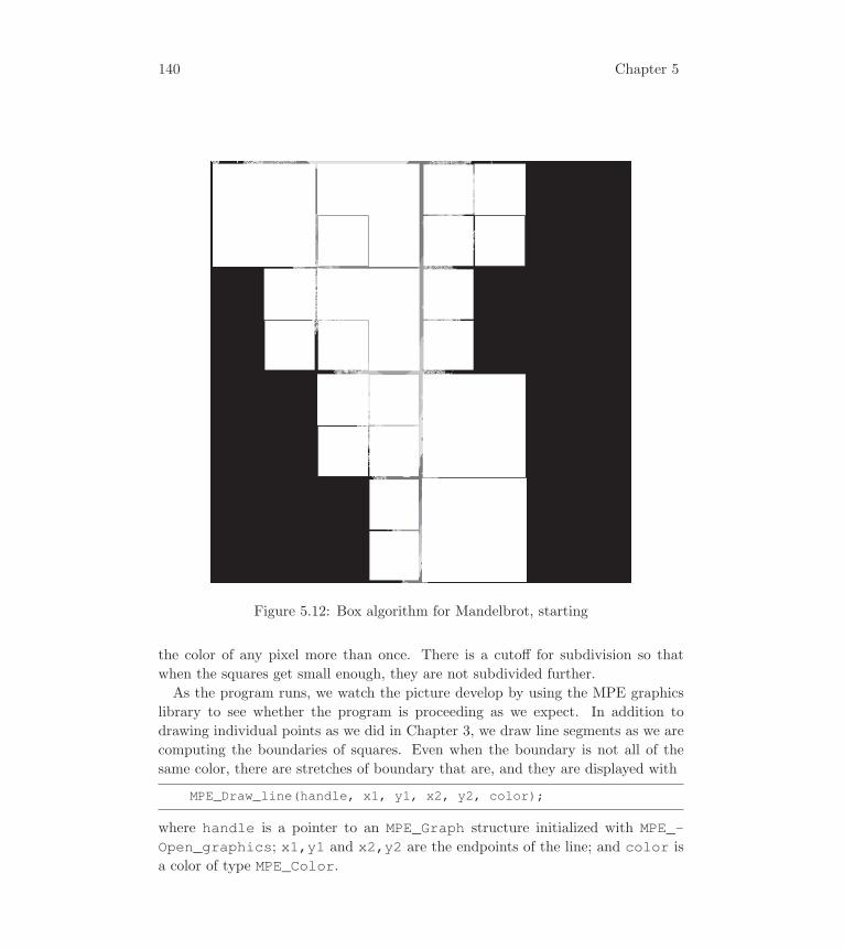
140 Chapter 5
Figure 5.12: Box algorithm for Mandelbrot, starting
the color of any pixel more than once. There is a cutoff for subdivision so that
when the squares get small enough, they are not subdivided further.
As the program runs, we watch the picture develop by using the MPE graphics
library to see whether the program is proceeding as we expect. In addition to
drawing individual points as we did in Chapter 3, we draw line segments as we are
computing the boundaries of squares. Even when the boundary is not all of the
same color, there are stretches of boundary that are, and they are displayed with
MPE_Draw_line(handle, x1, y1, x2, y2, color);
where handle is a pointer to an MPE_Graph structure initialized with MPE_-Open_graphics; x1,y1 and x2,y2 are the endpoints of the line; and color is
a color of type MPE_Color.
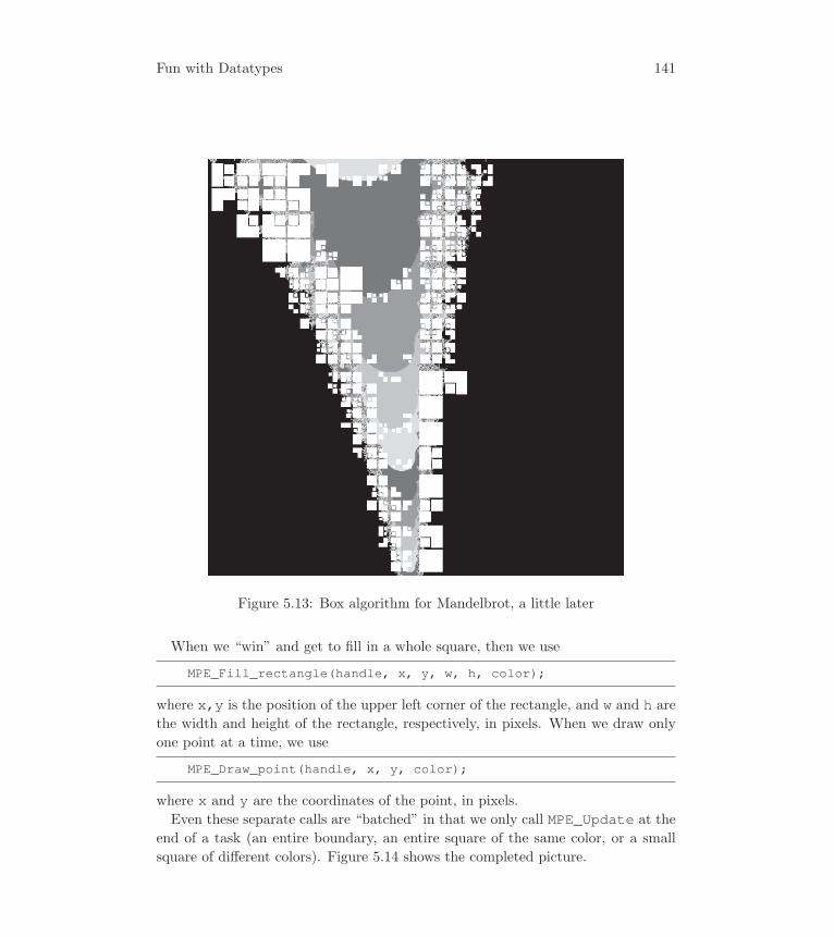
Fun with Datatypes 141
Figure 5.13: Box algorithm for Mandelbrot, a little later
When we “win” and get to fill in a whole square, then we use
MPE_Fill_rectangle(handle, x, y, w, h, color);
where x,y is the position of the upper left corner of the rectangle, and w and h are
the width and height of the rectangle, respectively, in pixels. When we draw only
one point at a time, we use
MPE_Draw_point(handle, x, y, color);
where x and y are the coordinates of the point, in pixels.
Even these separate calls are “batched” in that we only call MPE_Update at the
end of a task (an entire boundary, an entire square of the same color, or a small
square of different colors). Figure 5.14 shows the completed picture.

142 Chapter 5
Figure 5.14: Mandelbrot, complete
We take this opportunity to introduce the most general of the MPI derived data-
types, which may be used for sending C structures or parts of them. The Man-
delbrot program data structures contain a C structure that holds command line
arguments, which specify a large number of options for the program. It is con-
venient to keep them in a structure so that they can easily be passed to various
subroutines. MPI does not specify that all processes have access to the command
line arguments through MPI_Init, so we broadcast them, assuming that at least
the process with rank 0 in MPI_COMM_WORLD does get them when the program is
started. After storing them in its copy of this structure, it broadcasts the structure
to the other processes. The structure itself looks like the following:
struct {char display[50]; /* Name of display */

Fun with Datatypes 143
int maxiter; /* max # of iterations */double xmin, ymin; /* lower left corner of rectangle */double xmax, ymax; /* upper right corner */int width; /* of display in pixels */int height; /* of display in pixels */
} cmdline;
We would like to broadcast this structure with a single MPI_Bcast, taking advan-
tage of MPI’s facilities for dealing with alignment, mixed types, and heterogeneous
communication. We show here two ways to do so.
MPI_Type_create_struct is very general. It allows us to describe with a
single datatype a collection of data items of various elementary and derived types.
It considers the data to be composed of a set of “blocks” of data, each of which has
a count and datatype associated with it and a location given as a displacement.
The code to set up to broadcast the above structure would look like the following:
/* set up 4 blocks */int blockcounts[4] = {50,1,4,2};MPI_Datatype types[4];MPI_Aint displs[4];MPI_Datatype cmdtype;
/* initialize types and displs with addresses of items */MPI_Get_address(&cmdline.display, &displs[0]);MPI_Get_address(&cmdline.maxiter, &displs[1]);MPI_Get_address(&cmdline.xmin, &displs[2]);MPI_Get_address(&cmdline.width, &displs[3]);types[0] = MPI_CHAR;types[1] = MPI_INT;types[2] = MPI_DOUBLE;types[3] = MPI_INT;
The blockcounts array indicates how many elements there are for each corre-
sponding type. In our example, we have char display[50], so the value of
blockcounts[0] is 50. blockcounts[1] is one, matching the single int that
is the next element (maxiter) in the structure. Following maxiter, there are
four double values, starting with xmin, so blockcounts[2] is 4. There are
also two int values, so blockcounts[3] is 2.Now we are ready to do the broadcast. First we adjust the displacement array
so that the displacements are offsets from the beginning of the structure; that is,
we make them relative to the beginning of the structure.
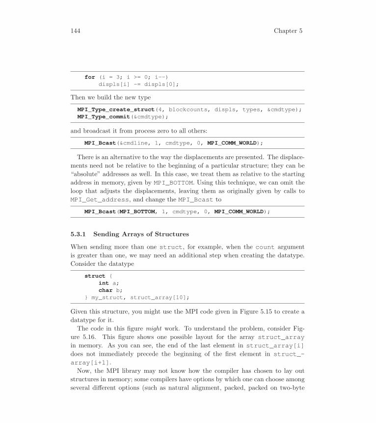
144 Chapter 5
for (i = 3; i >= 0; i--)displs[i] -= displs[0];
Then we build the new type
MPI_Type_create_struct(4, blockcounts, displs, types, &cmdtype);MPI_Type_commit(&cmdtype);
and broadcast it from process zero to all others:
MPI_Bcast(&cmdline, 1, cmdtype, 0, MPI_COMM_WORLD);
There is an alternative to the way the displacements are presented. The displace-
ments need not be relative to the beginning of a particular structure; they can be
“absolute” addresses as well. In this case, we treat them as relative to the starting
address in memory, given by MPI_BOTTOM. Using this technique, we can omit the
loop that adjusts the displacements, leaving them as originally given by calls to
MPI_Get_address, and change the MPI_Bcast to
MPI_Bcast(MPI_BOTTOM, 1, cmdtype, 0, MPI_COMM_WORLD);
5.3.1 Sending Arrays of Structures
When sending more than one struct, for example, when the count argument
is greater than one, we may need an additional step when creating the datatype.
Consider the datatype
struct {int a;char b;
} my_struct, struct_array[10];
Given this structure, you might use the MPI code given in Figure 5.15 to create a
datatype for it.
The code in this figure might work. To understand the problem, consider Fig-
ure 5.16. This figure shows one possible layout for the array struct_arrayin memory. As you can see, the end of the last element in struct_array[i]does not immediately precede the beginning of the first element in struct_-array[i+1].Now, the MPI library may not know how the compiler has chosen to lay out
structures in memory; some compilers have options by which one can choose among
several different options (such as natural alignment, packed, packed on two-byte
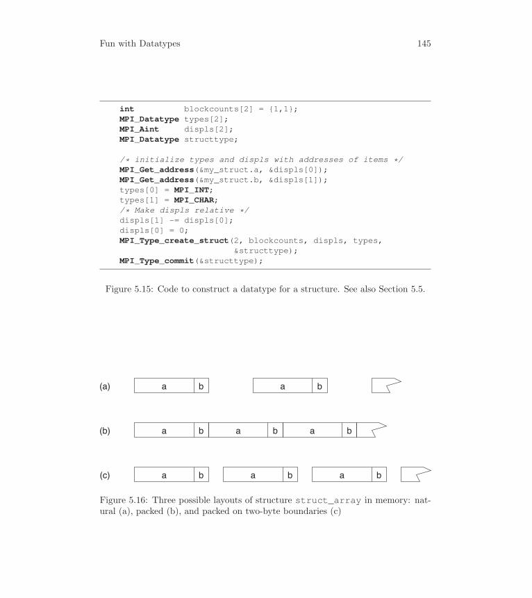
Fun with Datatypes 145
int blockcounts[2] = {1,1};MPI_Datatype types[2];MPI_Aint displs[2];MPI_Datatype structtype;
/* initialize types and displs with addresses of items */MPI_Get_address(&my_struct.a, &displs[0]);MPI_Get_address(&my_struct.b, &displs[1]);types[0] = MPI_INT;types[1] = MPI_CHAR;/* Make displs relative */displs[1] -= displs[0];displs[0] = 0;MPI_Type_create_struct(2, blockcounts, displs, types,
&structtype);MPI_Type_commit(&structtype);
Figure 5.15: Code to construct a datatype for a structure. See also Section 5.5.
ba ba
ba ba
ba ba
ba
ba
(a)
(b)
(c)
Figure 5.16: Three possible layouts of structure struct_array in memory: nat-ural (a), packed (b), and packed on two-byte boundaries (c)
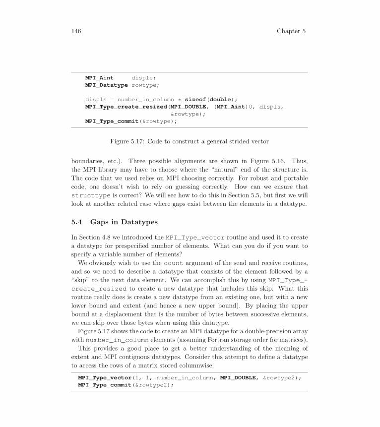
146 Chapter 5
MPI_Aint displs;MPI_Datatype rowtype;
displs = number_in_column * sizeof(double);MPI_Type_create_resized(MPI_DOUBLE, (MPI_Aint)0, displs,
&rowtype);MPI_Type_commit(&rowtype);
Figure 5.17: Code to construct a general strided vector
boundaries, etc.). Three possible alignments are shown in Figure 5.16. Thus,
the MPI library may have to choose where the “natural” end of the structure is.
The code that we used relies on MPI choosing correctly. For robust and portable
code, one doesn’t wish to rely on guessing correctly. How can we ensure that
structtype is correct? We will see how to do this in Section 5.5, but first we will
look at another related case where gaps exist between the elements in a datatype.
5.4 Gaps in Datatypes
In Section 4.8 we introduced the MPI_Type_vector routine and used it to create
a datatype for prespecified number of elements. What can you do if you want to
specify a variable number of elements?
We obviously wish to use the count argument of the send and receive routines,
and so we need to describe a datatype that consists of the element followed by a
“skip” to the next data element. We can accomplish this by using MPI_Type_-create_resized to create a new datatype that includes this skip. What this
routine really does is create a new datatype from an existing one, but with a new
lower bound and extent (and hence a new upper bound). By placing the upper
bound at a displacement that is the number of bytes between successive elements,
we can skip over those bytes when using this datatype.
Figure 5.17 shows the code to create an MPI datatype for a double-precision array
with number_in_column elements (assuming Fortran storage order for matrices).
This provides a good place to get a better understanding of the meaning of
extent and MPI contiguous datatypes. Consider this attempt to define a datatype
to access the rows of a matrix stored columnwise:
MPI_Type_vector(1, 1, number_in_column, MPI_DOUBLE, &rowtype2);MPI_Type_commit(&rowtype2);
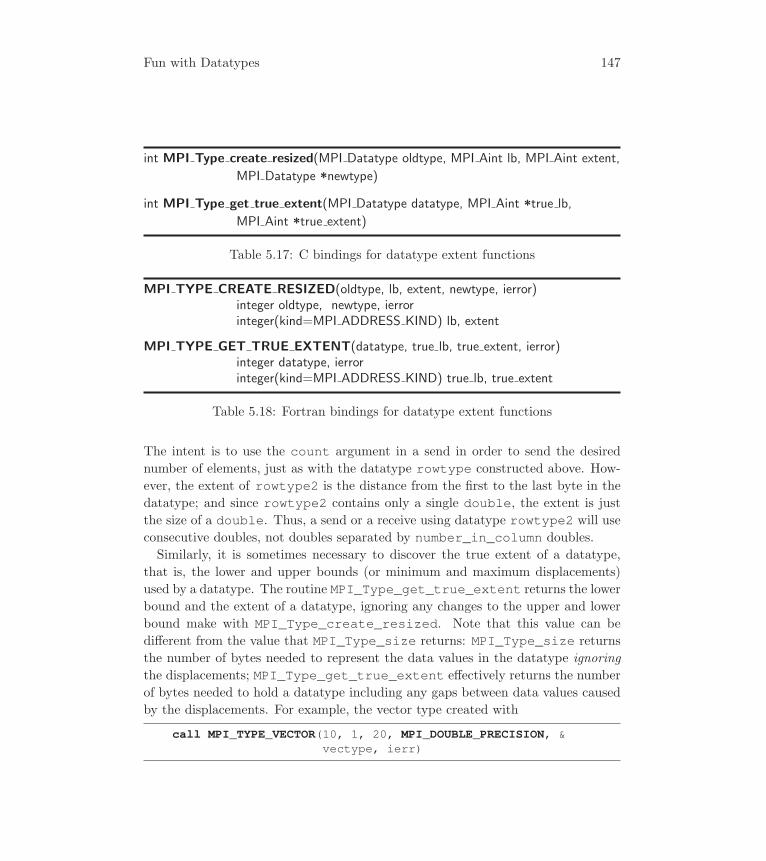
Fun with Datatypes 147
int MPI Type create resized(MPI Datatype oldtype, MPI Aint lb, MPI Aint extent,
MPI Datatype *newtype)
int MPI Type get true extent(MPI Datatype datatype, MPI Aint *true lb,
MPI Aint *true extent)
Table 5.17: C bindings for datatype extent functions
MPI TYPE CREATE RESIZED(oldtype, lb, extent, newtype, ierror)integer oldtype, newtype, ierrorinteger(kind=MPI ADDRESS KIND) lb, extent
MPI TYPE GET TRUE EXTENT(datatype, true lb, true extent, ierror)integer datatype, ierrorinteger(kind=MPI ADDRESS KIND) true lb, true extent
Table 5.18: Fortran bindings for datatype extent functions
The intent is to use the count argument in a send in order to send the desired
number of elements, just as with the datatype rowtype constructed above. How-
ever, the extent of rowtype2 is the distance from the first to the last byte in the
datatype; and since rowtype2 contains only a single double, the extent is just
the size of a double. Thus, a send or a receive using datatype rowtype2 will use
consecutive doubles, not doubles separated by number_in_column doubles.
Similarly, it is sometimes necessary to discover the true extent of a datatype,
that is, the lower and upper bounds (or minimum and maximum displacements)
used by a datatype. The routine MPI_Type_get_true_extent returns the lower
bound and the extent of a datatype, ignoring any changes to the upper and lower
bound make with MPI_Type_create_resized. Note that this value can be
different from the value that MPI_Type_size returns: MPI_Type_size returns
the number of bytes needed to represent the data values in the datatype ignoring
the displacements; MPI_Type_get_true_extent effectively returns the number
of bytes needed to hold a datatype including any gaps between data values caused
by the displacements. For example, the vector type created with
call MPI_TYPE_VECTOR(10, 1, 20, MPI_DOUBLE_PRECISION, &vectype, ierr)

148 Chapter 5
int blockcounts[2] = {1,1};MPI_Datatype types[2];MPI_Aint displs[2], s_lb, s_extent;MPI_Datatype structtype;
/* initialize types and displs with addresses of items */MPI_Get_address(&struct_array[0].a, &displs[0]);MPI_Get_address(&struct_array[0].b, &displs[1]);types[0] = MPI_INT;types[1] = MPI_CHAR;/* Make displs relative */displs[1] -= displs[0];displs[0] = 0;MPI_Type_create_struct(2, blockcounts, displs, types,
&structtype);/* Check that the datatype has the correct extent */MPI_Type_get_extent(structtype, &s_lb, &s_extent);if (s_extent != sizeof(struct_array[0])) {
MPI_Datatype sold = structtype;MPI_Type_create_resized(sold, 0, sizeof(my_struct),
&structtype);MPI_Type_free(&sold);
}MPI_Type_commit(&structtype);
Figure 5.18: Code to construct a datatype for a structure that does not rely onMPI using the same rule for structure padding as the C compiler
containing ten double precision values separated by a stride of 20 has a size (from
MPI_Type_size) of 80 bytes (assuming 8 byte DOUBLE PRECISION) and a true
extent of 1440 ( = (10− 1)× 20× 8 + 8 ) bytes.
5.5 More on Datatypes for Structures
Now that we have seen how to specify a gap at the end of a datatype, we can see
how to make the create a datatype for the structtype example in Figure 5.15.
We do this in two steps. First, create an MPI datatype that describes the elements
of the structure. Second, resize that type to have the correct extent if necessary;
that is, if the extent of MPI datatype created with MPI_Type_create_structis not the same as the sizeof the type in C. This is shown in Figure 5.18.
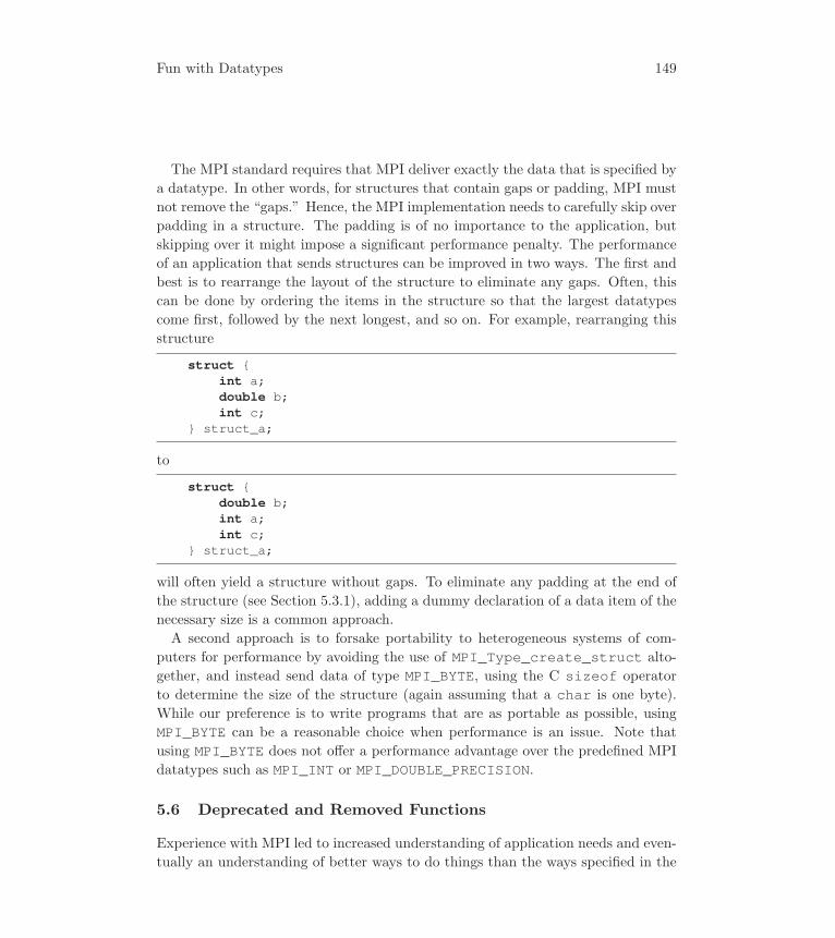
Fun with Datatypes 149
The MPI standard requires that MPI deliver exactly the data that is specified by
a datatype. In other words, for structures that contain gaps or padding, MPI must
not remove the “gaps.” Hence, the MPI implementation needs to carefully skip over
padding in a structure. The padding is of no importance to the application, but
skipping over it might impose a significant performance penalty. The performance
of an application that sends structures can be improved in two ways. The first and
best is to rearrange the layout of the structure to eliminate any gaps. Often, this
can be done by ordering the items in the structure so that the largest datatypes
come first, followed by the next longest, and so on. For example, rearranging this
structure
struct {int a;double b;int c;
} struct_a;
to
struct {double b;int a;int c;
} struct_a;
will often yield a structure without gaps. To eliminate any padding at the end of
the structure (see Section 5.3.1), adding a dummy declaration of a data item of the
necessary size is a common approach.
A second approach is to forsake portability to heterogeneous systems of com-
puters for performance by avoiding the use of MPI_Type_create_struct alto-
gether, and instead send data of type MPI_BYTE, using the C sizeof operator
to determine the size of the structure (again assuming that a char is one byte).
While our preference is to write programs that are as portable as possible, using
MPI_BYTE can be a reasonable choice when performance is an issue. Note that
using MPI_BYTE does not offer a performance advantage over the predefined MPI
datatypes such as MPI_INT or MPI_DOUBLE_PRECISION.
5.6 Deprecated and Removed Functions
Experience with MPI led to increased understanding of application needs and even-
tually an understanding of better ways to do things than the ways specified in the
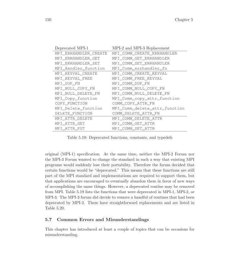
150 Chapter 5
Deprecated MPI-1 MPI-2 and MPI-3 ReplacementMPI_ERRHANDLER_CREATE MPI_COMM_CREATE_ERRHANDLERMPI_ERRHANDLER_GET MPI_COMM_GET_ERRHANDLERMPI_ERRHANDLER_SET MPI_COMM_SET_ERRHANDLERMPI_Handler_function MPI_Comm_errhandler_fnMPI_KEYVAL_CREATE MPI_COMM_CREATE_KEYVALMPI_KEYVAL_FREE MPI_COMM_FREE_KEYVALMPI_DUP_FN MPI_COMM_DUP_FNMPI_NULL_COPY_FN MPI_COMM_NULL_COPY_FNMPI_NULL_DELETE_FN MPI_COMM_NULL_DELETE_FNMPI_Copy_function MPI_Comm_copy_attr_functionCOPY_FUNCTION COMM_COPY_ATTR_FNMPI_Delete_function MPI_Comm_delete_attr_functionDELETE_FUNCTION COMM_DELETE_ATTR_FNMPI_ATTR_DELETE MPI_COMM_DELETE_ATTRMPI_ATTR_GET MPI_COMM_GET_ATTRMPI_ATTR_PUT MPI_COMM_SET_ATTR
Table 5.19: Deprecated functions, constants, and typedefs
original (MPI-1) specification. At the same time, neither the MPI-2 Forum nor
the MPI-3 Forum wanted to change the standard in such a way that existing MPI
programs would suddenly lose their portability. Therefore the forum decided that
certain functions would be “deprecated.” This means that these functions are still
part of the MPI standard and implementations are required to support them, but
that applications are encouraged to eventually abandon them in favor of new ways
of accomplishing the same things. However, a deprecated routine may be removed
from MPI. Table 5.19 lists the functions that were deprecated in MPI-1, MPI-2, or
MPI-3. The MPI-3 forum did decide to remove a handful of routines that had been
deprecated by MPI-2. These have straightforward replacements and are listed in
Table 5.20.
5.7 Common Errors and Misunderstandings
This chapter has introduced at least a couple of topics that can be occasions for
misunderstanding.
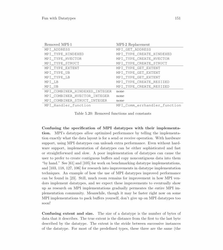
Fun with Datatypes 151
Removed MPI-1 MPI-2 ReplacementMPI_ADDRESS MPI_GET_ADDRESSMPI_TYPE_HINDEXED MPI_TYPE_CREATE_HINDEXEDMPI_TYPE_HVECTOR MPI_TYPE_CREATE_HVECTORMPI_TYPE_STRUCT MPI_TYPE_CREATE_STRUCTMPI_TYPE_EXTENT MPI_TYPE_GET_EXTENTMPI_TYPE_UB MPI_TYPE_GET_EXTENTMPI_TYPE_LB MPI_TYPE_GET_EXTENTMPI_LB MPI_TYPE_CREATE_RESIZEDMPI_UB MPI_TYPE_CREATE_RESIZEDMPI_COMBINER_HINDEXED_INTEGER noneMPI_COMBINER_HVECTOR_INTEGER noneMPI_COMBINER_STRUCT_INTEGER noneMPI_Handler_function MPI_Comm_errhandler_function
Table 5.20: Removed functions and constants
Confusing the specification of MPI datatypes with their implementa-
tion. MPI’s datatypes allow optimized performance by telling the implementa-
tion exactly what the data layout is for a send or receive operation. With hardware
support, using MPI datatypes can unleash extra performance. Even without hard-
ware support, implementation of datatypes can be either sophisticated and fast
or straightforward and slow. A poor implementation of datatypes can cause the
user to prefer to create contiguous buffers and copy noncontiguous data into them
“by hand.” See [61] and [105] for work on benchmarking datatype implementations,
and [103, 118, 127, 106] for research into improvements in datatype implementation
techniques. An example of how the use of MPI datatypes improved performance
can be found in [23]. Still, much room remains for improvement in how MPI ven-
dors implement datatypes, and we expect these improvements to eventually show
up as research on MPI implementations gradually permeates the entire MPI im-
plementation community. Meanwhile, though it may be faster right now on some
MPI implementations to pack buffers yourself, don’t give up on MPI datatypes too
soon!
Confusing extent and size. The size of a datatype is the number of bytes of
data that it describes. The true extent is the distance from the first to the last byte
described by the datatype. The extent is the stride between successive instances
of the datatype. For most of the predefined types, these three are the same (the
152 Chapter 5
predefined datatypes for the MPI_MAXLOC and MPI_MINLOC operators may be
exceptions, depending on the underlying compiler and hardware). But for many
user-constructed datatypes, the size and extent will be different. See the end of
Section 5.1 for more details.
5.8 Application: Cosmological Large-Scale Structure Formation
Our application for this chapter is a more sophisticated approach to the N-body
problem that we introduced here.
The early history of the universe was characterized by a hot phase, after which
the continuing expansion of the universe led to a cooling of its constituents. The
matter component—mostly dark matter—began to collapse under its own mutual
gravitational attraction. Various statistical properties of the structure that results
from this collapse are functions of statistical properties of the initial matter configu-
ration, and these in turn are functions of some aspects of fundamental physics—the
true target of investigation. Moreover, these same statistical properties can be mea-
sured in our real universe by using surveys conducted with large telescopes. Because
gravitational collapse is a highly nonlinear process, the relationship between these
statistical properties of the initial conditions and those at later times can be de-
termined only by numerical simulation. Hence, numerical simulation results are
necessary in order to derive constraints on fundamental physics from the statistics
derived from observational data.
Inside the simulation, the universe’s matter is represented by using a collection of
homogeneous particles interacting via the force of gravity. Cosmologists often use
the astronomical unit of “parsec” (abbreviated pc) to measure distances; 1 pc is
approximately 3.26 light years. In order to match the volume of large-scale surveys,
the simulation must be a few gigaparsecs on each side. And in order to gather
measurements from the simulation with sufficiently low statistical uncertainty, each
particle can be only about 108 solar masses. Thus, modern simulations will require
trillions of particles. Using the direct O(N2) algorithm to compute the gravitational
force of every particle on every other would be hopeless on any computer, but
more efficient algorithms exist. HACC, a simulation developed at Los Alamos and
Argonne National Laboratories, can conduct simulations of such astronomical size
by decomposing this interparticle force calculation into several different pieces.
On the largest scales, the interparticle force is computed by depositing each
particle’s mass on a large, distributed grid and then using a method that takes
advantage of the fast Fourier transform (FFT) in order to compute the force in
O(M logM) time. M is the number of grid cells, and generally M is chosen equal
Fun with Datatypes 153
to (or more than) the total number of particles. Unfortunately, the resulting force
computation is accurate only to the size of the grid; and because the particles
cluster together, having only grid-scale force resolution is insufficient to accurately
predict the particle motions. In order to gain finer force resolution, an additional
force solver is used for the small-scale residual force. The best mechanism to use to
construct such a high-resolution solver depends on the computer architecture. For
systems with GPU accelerators, the directN2 residual is computed. For CPU-based
systems, the force is further approximated by using a multipole-like method built on
top of a k-dimensional treelike data structure. This data structure recursively sorts
the particles based on their spatial coordinates and then approximates the force
on each particle from groups of relatively distant particles. In order to keep this
high-resolution piece of the calculation local to each MPI rank, each rank maintains
a large ghost region of particles from neighboring ranks.
HACC exhibits two kinds of interrank communication: all-to-all communication
for the FFT and neighbor-to-neighbor when exchanging ghost zones of grid force
and particles. Both these communication phases can be accomplished efficiently,
even on the largest modern supercomputers (see Figure 5.19). The result is that
HACC can perform the needed trillion-particle simulations necessary to advance
cosmology in conjunction with modern observational advances.
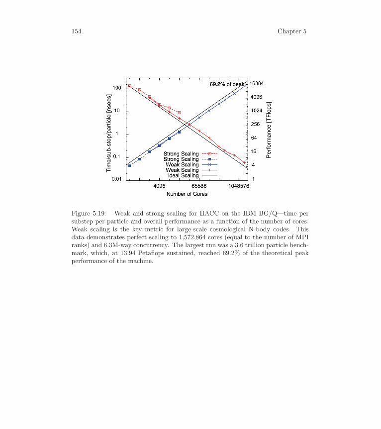
154 Chapter 5
Figure 5.19: Weak and strong scaling for HACC on the IBM BG/Q—time persubstep per particle and overall performance as a function of the number of cores.Weak scaling is the key metric for large-scale cosmological N-body codes. Thisdata demonstrates perfect scaling to 1,572,864 cores (equal to the number of MPIranks) and 6.3M-way concurrency. The largest run was a 3.6 trillion particle bench-mark, which, at 13.94 Petaflops sustained, reached 69.2% of the theoretical peakperformance of the machine.
6 Parallel Libraries
One of the primary motivations for MPI was to enable the development of par-
allel libraries. Libraries have been critical to the development of a software base
for sequential computers. Lack of modularity in the first generation of message-
passing systems hampered the comparable development of reliable parallel libraries,
libraries that can be written independently of one another and of user code and
still cooperate with one another in a single application.
We begin this chapter with a discussion of some of the issues that are raised by
parallel libraries. We describe some of the shortcomings of early message-passing
systems when they are considered from the viewpoint of the library writer, and we
point out features of the MPI definition that were introduced to overcome these
shortcomings. We then give an example of a simple library; it contains only two
functions but illustrates a number of MPI’s features that support libraries. We
devote a section to the interplay between linear algebra and partial differential
equations as an example of an area where parallel libraries are likely to be heavily
used. We briefly describe some aspects of the use of MPI in the solution of a dense
system of linear equations. We conclude the chapter with a discussion of general
strategies for building parallel libraries.
6.1 Motivation
In this section we outline the motivation for libraries and describe the special design
features of MPI that help in building parallel libraries.
6.1.1 The Need for Parallel Libraries
Software libraries offer several advantages:
• They ensure consistency in program correctness.
• They help guarantee a high-quality implementation.
• They hide distracting details and complexities associated with state-of-the-art
implementations.
• They minimize repetitive effort or haphazard results.
Even in sequential libraries, library writers incorporate numerous heuristics and
domain-specific “tricks.” With the addition of parallelism based on message pass-
ing, the “detail work” of typical numerical methods grows significantly, strongly

156 Chapter 6
motivating the development of parallel libraries that encapsulate and hide this
complexity from the user. MPI is the underlying system library that will help
make scientific as well as application-oriented parallel libraries both reliable and
commonplace.
6.1.2 Common Deficiencies of Early Message-Passing Systems
In the sequential Fortran and C environments, one can easily create libraries, be-
cause the stack-oriented procedural programming model has well-defined conditions
about reasonable vs. erroneous programs. In the distributed-memory, message-
passing environment, however, libraries are difficult to write with either vendor-
supplied software or portability systems. The problem is one of modularity: a
library needs a communication space isolated from the user’s communication space
precisely because it is a library. Its communication patterns are designed indepen-
dently of the user code it is to be linked to.
The most obvious problem is that of having a message sent by the library acci-
dentally received by user code, or vice versa. One might argue that tags could be
used effectively to designate restrictions on message delivery. Such tags prove insuf-
ficient, however, for several reasons. First, more than one library (or invocation of
the same library) could use the same tags. Second, wildcard receipt-selectivity on
tags (e.g., MPI_ANY_TAG) destroys any promise of real protection that tags could
otherwise afford. For this reason parallel libraries are often written in a style that
strictly alternates execution of user code and library code, with care taken that no
messages be in transit when control is passed from user to library and back (this
state is often called quiescence). This type of design, inherited from the sequential
case, introduces synchronization barriers that inhibit performance, and still leaves
other problems unsolved.
This problem can be illustrated with a simple example. Let’s assume that the
program calls two routines, SendRight and SendEnd. These two routines are
shown in Figure 6.1. Two possible execution sequences for these routines are shown
in Figure 6.2. In part (b) of this figure, the messages are received by the wrong
routine because the message from routine SendEnd on process zero arrives at
process two before the message from SendRight on process one arrives at process
two. This example depends on using MPI_ANY_SOURCE in both of the routines.
While in this case the routines could be written to provide an explicit source instead,
in other cases (particularly manager/worker examples), MPI_ANY_SOURCE cannot
be avoided.
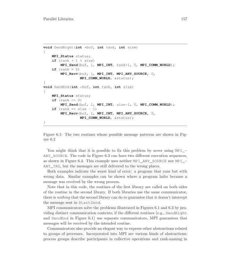
Parallel Libraries 157
void SendRight(int *buf, int rank, int size){
MPI_Status status;if (rank + 1 < size)
MPI_Send(buf, 1, MPI_INT, rank+1, 0, MPI_COMM_WORLD);if (rank > 0)
MPI_Recv(buf, 1, MPI_INT, MPI_ANY_SOURCE, 0,MPI_COMM_WORLD, &status);
}void SendEnd(int *buf, int rank, int size){
MPI_Status status;if (rank == 0)
MPI_Send(buf, 1, MPI_INT, size-1, 0, MPI_COMM_WORLD);if (rank == size - 1)
MPI_Recv(buf, 1, MPI_INT, MPI_ANY_SOURCE, 0,MPI_COMM_WORLD, &status);
}
Figure 6.1: The two routines whose possible message patterns are shown in Fig-ure 6.2
You might think that it is possible to fix this problem by never using MPI_-ANY_SOURCE. The code in Figure 6.3 can have two different execution sequences,
as shown in Figure 6.4. This example uses neither MPI_ANY_SOURCE nor MPI_-ANY_TAG, but the messages are still delivered to the wrong places.
Both examples indicate the worst kind of error: a program that runs but with
wrong data. Similar examples can be shown where a program halts because a
message was received by the wrong process.
Note that in this code, the routines of the first library are called on both sides
of the routine in the second library. If both libraries use the same communicator,
there is nothing that the second library can do to guarantee that it doesn’t intercept
the message sent in StartSend.MPI communicators solve the problems illustrated in Figures 6.1 and 6.3 by pro-
viding distinct communication contexts; if the different routines (e.g., SendRightand SendEnd in Figure 6.1) use separate communicators, MPI guarantees that
messages will be received by the intended routine.
Communicators also provide an elegant way to express other abstractions related
to groups of processes. Incorporated into MPI are various kinds of abstractions:
process groups describe participants in collective operations and rank-naming in
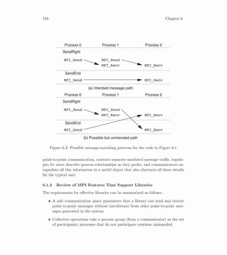
158 Chapter 6
MPI_Send MPI_Recv
(a) Intended message path
Process 0 Process 1 Process 2
SendRight
SendEnd
MPI_Send
MPI_RecvMPI_Recv
MPI_Send
MPI_Send MPI_Recv
(b) Possible but unintended path
Process 0 Process 1 Process 2
SendRight
SendEnd
MPI_Send
MPI_RecvMPI_Recv
MPI_Send
Figure 6.2: Possible message-matching patterns for the code in Figure 6.1
point-to-point communication, contexts separate unrelated message traffic, topolo-
gies let users describe process relationships as they prefer, and communicators en-
capsulate all this information in a useful object that also abstracts all these details
for the typical user.
6.1.3 Review of MPI Features That Support Libraries
The requirements for effective libraries can be summarized as follows:
• A safe communication space guarantees that a library can send and receive
point-to-point messages without interference from other point-to-point mes-
sages generated in the system.
• Collective operations take a process group (from a communicator) as the set
of participants; processes that do not participate continue unimpeded.

Parallel Libraries 159
/* Code for library 1: Nonblocking send from 0 to 1 */void StartSend(int *buf, int rank, int size, MPI_Request *req){
if (rank == 0)MPI_Isend(buf, 1, MPI_INT, 1, 0, MPI_COMM_WORLD, req);
}
void EndSend(int *buf, int rank, MPI_Request *req){
if (rank == 0)MPI_Wait(req, MPI_STATUS_IGNORE);
else if (rank == 1)MPI_Recv(buf, 1, MPI_INT, 0, 0, MPI_COMM_WORLD,
MPI_STATUS_IGNORE);}
/* Code for library 2: send from 0 to 1 */void DoSomething(int *buf, int rank, int size){
if (rank == 0)MPI_Send(buf, 1, MPI_INT, 1, 0, MPI_COMM_WORLD);
else if (rank == 1)MPI_Recv(buf, 1, MPI_INT, 0, 0, MPI_COMM_WORLD,
MPI_STATUS_IGNORE);}
Figure 6.3: Code whose message pattern is shown in Figure 6.4
• Abstract names for processes are based on virtual topologies, or at least rank-
in-group names, thereby avoiding hardware dependencies, and ideally making
application code more intuitive.
MPI offers several features that implement these important requirements:
• Process groups define a rank-naming for processes in point-to-point com-
munication relative to the group. In addition, these groups define the scope of
collective operations. (Note that the internal representations of process names
are not revealed at the application level; that would spoil portability.) This
scope makes it possible to make strong statements about the noninterference
of sequential collective operations in the same communication context.
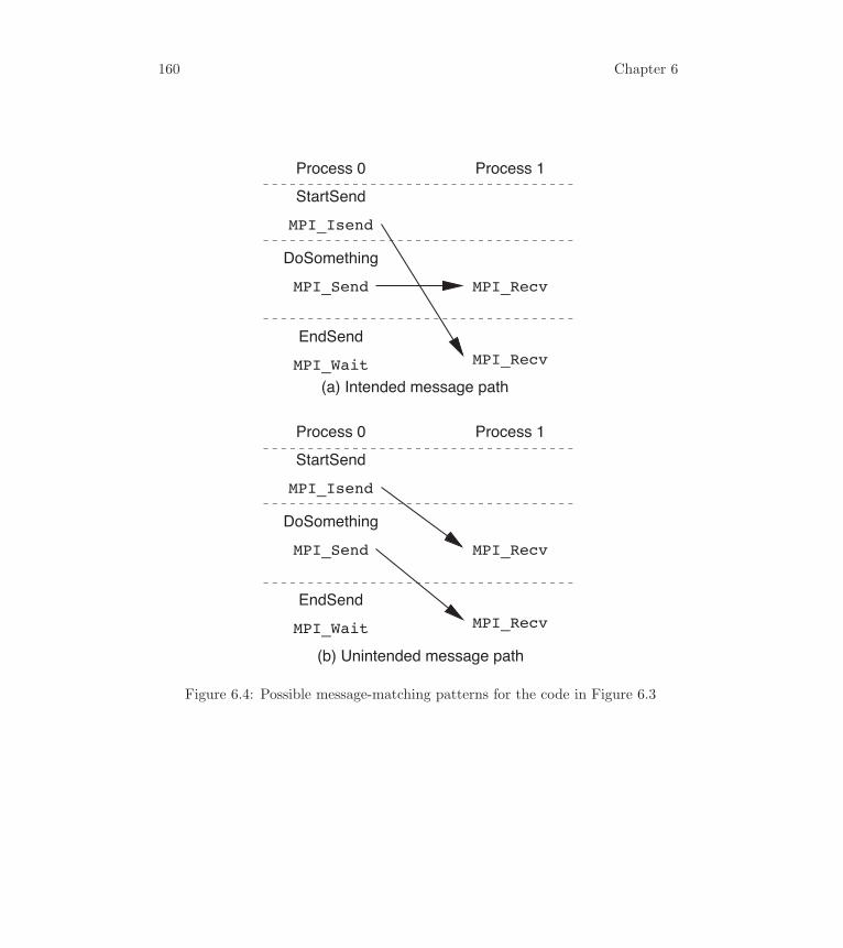
160 Chapter 6
Process 0 Process 1
MPI_Isend
MPI_Recv
StartSend
EndSend
DoSomething
MPI_Send MPI_Recv
MPI_Wait
Process 0 Process 1
MPI_Isend
MPI_Recv
StartSend
EndSend
DoSomething
MPI_Send MPI_Recv
MPI_Wait
(a) Intended message path
(b) Unintended message path
Figure 6.4: Possible message-matching patterns for the code in Figure 6.3

Parallel Libraries 161
• Contexts provide the ability to have separate safe “universes” (called con-
texts) of message passing in MPI. A context is conceptually implemented
by a secondary or “hyper” tag that differentiates messages from one another.
Unlike user-manipulated tags, these contexts provide totally separate commu-
nication space, each with a full complement of user-managed tags. Contexts
are allocated by the system for safety; if users were to define contexts, two
libraries might inadvertently define the same one. Users do not work directly
with contexts; rather, they work with process groups and communicators.
• Communicators encapsulate contexts, groups, and virtual topologies in an
object that provides the appropriate scope for all communication operations in
MPI. Communicators bind process groups and context information together
to form a safe communication space within the group. The communicator also
provides an object that can be used to maintain local (to the communicator)
copies of data that the library needs to keep from one invocation to another.
The MPI term for this is “attribute caching.”
The use of separate communication contexts by distinct libraries (or distinct
library invocations) insulates communication internal to the library execution
from external communication (group safety). This approach allows one to
invoke the library even if communications are pending. Moreover, it avoids
the need to synchronize each entry into and exit from library code. Most such
synchronizations are unnecessary, reduce performance, and can be avoided
because of the context model.
6.2 A First MPI Library
In this section we describe a simple two-function library. It provides a feature not
included in MPI: a way to execute a block of code sequentially, one process at a
time. This can be useful when generating output to a file or to standard output,
for example. Use of this library is illustrated with the following example:
seqBegin(MPI_COMM_WORLD);printf("My rank is %d\n", wrank);fflush(stdout);seqEnd(MPI_COMM_WORLD);
Note the use of fflush—without this, the C library implementation of printfmay buffer the output and not send it to standard output until more output text
has been accumulated. We also note that whether this data appears on standard
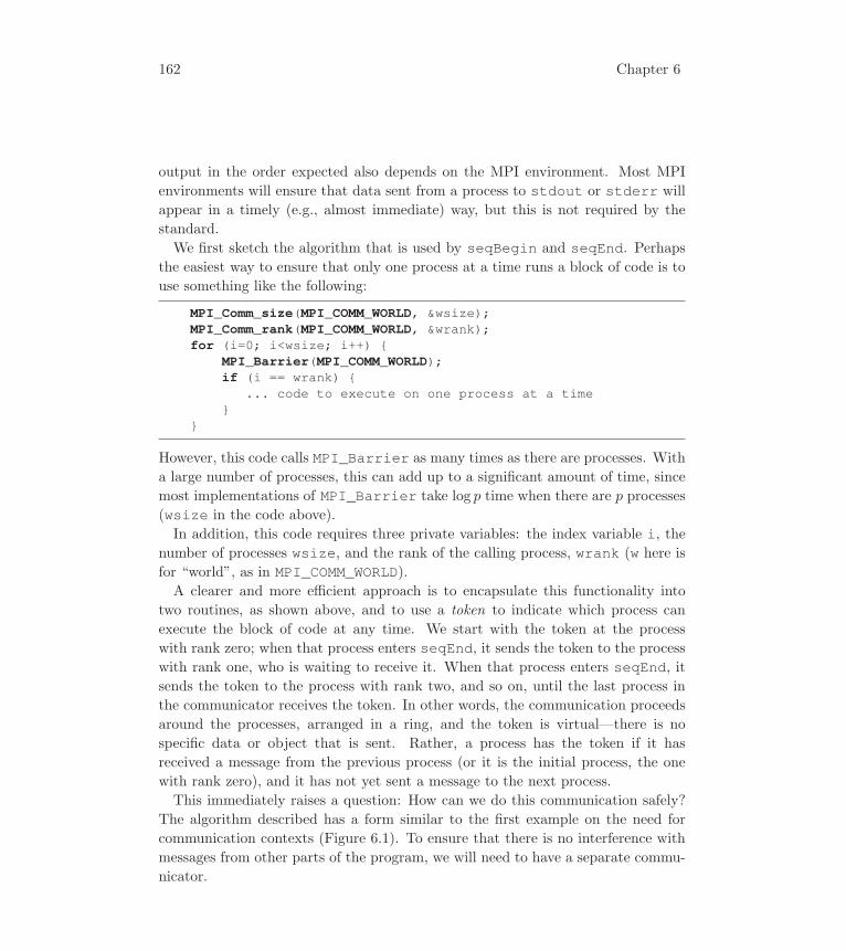
162 Chapter 6
output in the order expected also depends on the MPI environment. Most MPI
environments will ensure that data sent from a process to stdout or stderr will
appear in a timely (e.g., almost immediate) way, but this is not required by the
standard.
We first sketch the algorithm that is used by seqBegin and seqEnd. Perhaps
the easiest way to ensure that only one process at a time runs a block of code is to
use something like the following:
MPI_Comm_size(MPI_COMM_WORLD, &wsize);MPI_Comm_rank(MPI_COMM_WORLD, &wrank);for (i=0; i<wsize; i++) {
MPI_Barrier(MPI_COMM_WORLD);if (i == wrank) {
... code to execute on one process at a time}
}
However, this code calls MPI_Barrier as many times as there are processes. With
a large number of processes, this can add up to a significant amount of time, since
most implementations of MPI_Barrier take log p time when there are p processes
(wsize in the code above).
In addition, this code requires three private variables: the index variable i, thenumber of processes wsize, and the rank of the calling process, wrank (w here is
for “world”, as in MPI_COMM_WORLD).A clearer and more efficient approach is to encapsulate this functionality into
two routines, as shown above, and to use a token to indicate which process can
execute the block of code at any time. We start with the token at the process
with rank zero; when that process enters seqEnd, it sends the token to the process
with rank one, who is waiting to receive it. When that process enters seqEnd, itsends the token to the process with rank two, and so on, until the last process in
the communicator receives the token. In other words, the communication proceeds
around the processes, arranged in a ring, and the token is virtual—there is no
specific data or object that is sent. Rather, a process has the token if it has
received a message from the previous process (or it is the initial process, the one
with rank zero), and it has not yet sent a message to the next process.
This immediately raises a question: How can we do this communication safely?
The algorithm described has a form similar to the first example on the need for
communication contexts (Figure 6.1). To ensure that there is no interference with
messages from other parts of the program, we will need to have a separate commu-
nicator.

Parallel Libraries 163
/* Sequential execution code */#include "mpi.h"#include <stdio.h>#include <stdlib.h>
typedef struct {MPI_Comm lcomm;int prevRank, nextRank;
} seqInfo;
static int seqKeyval = MPI_KEYVAL_INVALID;
Figure 6.5: The header file for seqBegin and seqEnd
We will take the following approach. For each input communicator (the MPI_-Comm argument to seqBegin), we will create a new, private communicator with
MPI_Comm_dup. We will also precompute the rank of the process from which we
receive the token and the rank of the process to which we will send the token. So
that we don’t do this every time seqBegin is called on the same communicator,
we’ll save this information. The C structure that holds this information is shown in
Figure 6.5 as seqInfo. But where can we save this value so that, when seqBeginis called with a communicator, we can find the appropriate private communicator
and communication ranks? We could keep a table of correspondences between
communicators that we have seen before and the private seqInfos that we have
created. But it would be better if we could somehow attach the seqInfo value
to the input communicator. Fortunately, MPI allows us to do just this. The MPI
term for this is caching of attributes, and it is typically used to keep a pointer
to a data structure used by the library to maintain information between calls. In
Fortran, it is an integer. Attributes are identified by key values, which are system
allocated so that multiple libraries can attach attributes to the same communicator
without knowledge of one another.
In this case the cached information includes a communicator to be used for
seqBegin’s internal communication and the ranks of the previous and next pro-
cesses in the communication ring. The seqInfo structure is shown in Figure 6.5.
The complete sequential execution library is shown in Figures 6.6 and 6.7. It
demonstrates how to use communicators and caching. The way that attributes
are attached to communicators allows for their selective propagation when the call
MPI_Comm_dup is used, as we define further in this example. The already-discussed

164 Chapter 6
call MPI_Comm_create never copies attributes to the newly created communica-
tor. The sequential execution library requires the use of caching to store persistent
information and it requires the use of a cached communicator to protect the user
from communication actions of the library. The code for seqBegin is shown in
Figure 6.6 and 6.7.
What’s going on in this library? First, seqBegin checks to see whether it has
ever been called before by this process, by seeing whether it has a valid value for the
global integer seqKeyval. If not, seqBegin has to get an attribute key value,
so that it can cache its information on this and all future communicators that
may call seqBegin in this process; it does so with MPI_Comm_create_keyval.Otherwise, seqBegin is already the key value for use by this library.
Next, the code checks to see whether an seqBegin has ever been called on the
current communicator, by looking up the attribute for the key value seqKeyval. Ifnot, the system handle associated with this key value is created and attached to the
communicator. The most notable call here is MPI_Comm_dup1 communicator, but
with new contexts of communication. Any “other” attributes cached by the system
will be selectively copied, according to the attribute-copying set up by the user
when those attributes were attached. (See Table 6.1 for the bindings for attribute
copying and deletion functions.) The next task for seqBegin is to determine all
the specific data that needs to go in the user handle for this particular call, so that
the work of transmitting data can begin and so that the user can also legally call
seqEnd.Processes that call this library are in one of three states: executing the sequential
block of code, waiting to receive the token, or waiting to complete the final MPI_-Barrier, which is necessary to ensure that successive uses of the library on the
same communicator maintain the guaranteed ordering of execution of the code
between the seqBegin and seqEnd calls.
In seqBegin, after the information saved in the attribute is accessed, every pro-
cess performs an MPI_Recv from rank prevRank. For the process with rank zero
in the communicator, the value of this is MPI_PROC_NULL;, and the MPI_Recvcall completes immediately, allowing the routine to finish and return to the user’s
code, which thus begins the execution of the code that the user wants executed
sequentially. The other processes wait.
1In MPI-3, there was a subtle change to communicators that makes it a better practice use aroutine new in MPI-3 for duplicating communicators. This routine is MPI_Comm_dup_with_info,which makes a complete duplicate of the input communicator but without copying any “info”values from the parent communicator. See Using Advanced MPI [55] for a more comprehensivediscussion.

Parallel Libraries 165
int MPI Comm dup(MPI Comm comm, MPI Comm *newcomm)
int MPI Comm create keyval(MPI Copy function *copy fn,
MPI Delete function *delete fn, int *keyval, void* extra state)
int MPI Comm set attr(MPI Comm comm, int keyval, void* attribute val)
int MPI Comm get attr(MPI Comm comm, int keyval, void* attribute val, int *flag)
int MPI Comm free keyval(int *keyval)
int MPI Comm delete attr(MPI Comm comm, int keyval)
typedef int MPI Comm copy attr function(MPI Comm oldcomm, int *keyval,
void *extra state, void *attribute value in, void *attribute value out,int *flag)
typedef int MPI Comm delete attr function(MPI Comm comm, int *keyval,
void *attribute value, void *extra state)
Table 6.1: C bindings for new MPI calls needed by seqBegin, seqEnd,and related calls. The attribute_value in MPI_Comm_get_attr is castas a void * to simplify casts; the actual argument must be a pointer to apointer of the correct type. The same applies to attribute_value_out inMPI_Comm_copy_attr_function.
Once a process completes the sequential block of code and enters seqEnd, itagain finds the attribute, extracts the information about the private communicator
and the rank of the next process, and sends the token to that process. If the process
is the last in the ring, the value of nextRank is MPI_PROC_NULL, and this send
returns immediately. All processes then enter MPI_Barrier, which ensures that
no sequential section can start until all processes are complete with the current one.
Communicators are frequently created by copying existing communicators (with
MPI_Comm_dup) and are eventually freed, at which point one might wish to clean
up storage associated with an attribute. In order to handle attached attributes
during these operations, MPI specifies that when a key value is created, the user
may supply functions to copy and delete the attribute value when the communicator
is copied or freed. In our example, we have specified the delete function; this is the
seqDelFn argument to MPI_Comm_create_keyval, and the implementation of
the delete function is shown in Figure 6.8.
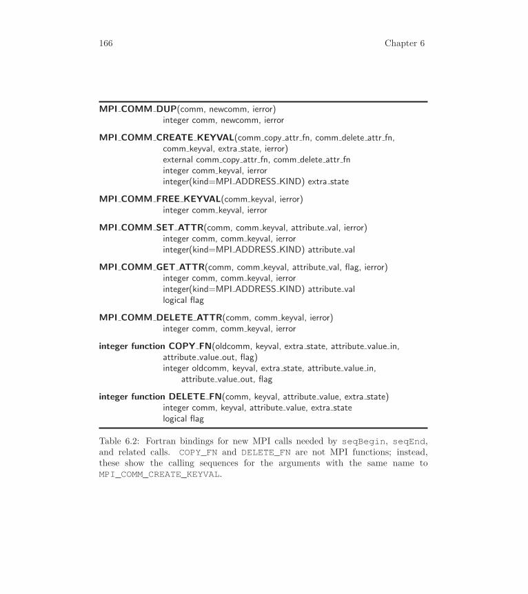
166 Chapter 6
MPI COMM DUP(comm, newcomm, ierror)integer comm, newcomm, ierror
MPI COMM CREATE KEYVAL(comm copy attr fn, comm delete attr fn,comm keyval, extra state, ierror)external comm copy attr fn, comm delete attr fninteger comm keyval, ierrorinteger(kind=MPI ADDRESS KIND) extra state
MPI COMM FREE KEYVAL(comm keyval, ierror)integer comm keyval, ierror
MPI COMM SET ATTR(comm, comm keyval, attribute val, ierror)integer comm, comm keyval, ierrorinteger(kind=MPI ADDRESS KIND) attribute val
MPI COMM GET ATTR(comm, comm keyval, attribute val, flag, ierror)integer comm, comm keyval, ierrorinteger(kind=MPI ADDRESS KIND) attribute vallogical flag
MPI COMM DELETE ATTR(comm, comm keyval, ierror)integer comm, comm keyval, ierror
integer function COPY FN(oldcomm, keyval, extra state, attribute value in,attribute value out, flag)integer oldcomm, keyval, extra state, attribute value in,
attribute value out, flag
integer function DELETE FN(comm, keyval, attribute value, extra state)integer comm, keyval, attribute value, extra statelogical flag
Table 6.2: Fortran bindings for new MPI calls needed by seqBegin, seqEnd,and related calls. COPY_FN and DELETE_FN are not MPI functions; instead,these show the calling sequences for the arguments with the same name toMPI_COMM_CREATE_KEYVAL.

Parallel Libraries 167
int seqDelFn(MPI_Comm comm, int keyval, void *attr, void *estate);
void seqBegin(MPI_Comm comm){
MPI_Comm lcomm;int flag, mysize, myrank;seqInfo *info;if (seqKeyval == MPI_KEYVAL_INVALID) {
MPI_Comm_create_keyval(MPI_NULL_COPY_FN, seqDelFn,&seqKeyval, NULL);
}MPI_Comm_get_attr(comm, seqKeyval, &info, &flag);if (!flag) {
info = (seqInfo *)malloc(sizeof(seqInfo));MPI_Comm_dup(comm, &info->lcomm);MPI_Comm_rank(info->lcomm, &myrank);MPI_Comm_size(info->lcomm, &mysize);info->prevRank = myrank - 1;if (info->prevRank < 0) info->prevRank = MPI_PROC_NULL;info->nextRank = myrank + 1;if (info->nextRank >= mysize) info->nextRank = MPI_PROC_NULL;MPI_Comm_set_attr(comm, seqKeyval, info);
}MPI_Recv(NULL, 0, MPI_INT, info->prevRank, 0, info->lcomm,
MPI_STATUS_IGNORE);}
Figure 6.6: Implementation of seqBegin
In some cases, a library may want to ensure that the cached attribute information
is propagated to new communicators created with MPI_Comm_dup. The version
of seqBegin in Figure 6.6 does not do this, but a simple change is all that is
required to add this feature. By changing one line of seqBegin, we can add the
copy callbacks:

168 Chapter 6
void seqEnd(MPI_Comm comm){
seqInfo *info;int flag;
/* Sanity check */if (seqKeyval == MPI_KEYVAL_INVALID)
MPI_Abort(MPI_COMM_WORLD, 1);MPI_Comm_get_attr(comm, seqKeyval, &info, &flag);if (!info || !flag)
MPI_Abort(MPI_COMM_WORLD, 1);
MPI_Send(NULL, 0, MPI_INT, info->nextRank, 0, info->lcomm);
/* Make everyone wait until all have completed their send */MPI_Barrier(info->lcomm);
}
Figure 6.7: Implementation of seqEnd
static int seqDelFn(MPI_Comm comm, int keyval, void *attr,void *estate)
{seqInfo *myinfo = (seqInfo *)attr;MPI_Comm_free(&myinfo->lcomm);free(myinfo);return 0;
}
Figure 6.8: Implementation of seqDelFn, the attribute delete function
/* first see if this library has ever been called. */if (seqKeyval == MPI_KEYVAL_INVALID) {
/* our first mission is to create the process-local keyvalfor this library, while specifying callbacks */
MPI_Comm_create_keyval(seqCopyFn, seqDelFn,&seqKeyval, NULL);
...
The implementation of the copy function is shown in Figure 6.9. This function
creates a new communicator with MPI_Comm_dup and uses the same ranks of
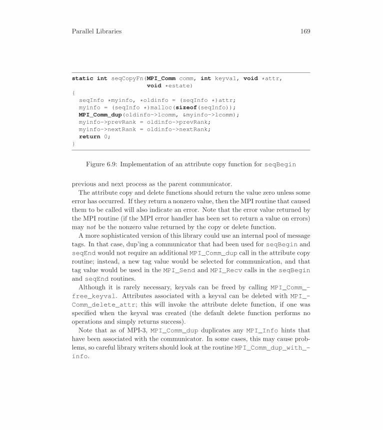
Parallel Libraries 169
static int seqCopyFn(MPI_Comm comm, int keyval, void *attr,void *estate)
{seqInfo *myinfo, *oldinfo = (seqInfo *)attr;myinfo = (seqInfo *)malloc(sizeof(seqInfo));MPI_Comm_dup(oldinfo->lcomm, &myinfo->lcomm);myinfo->prevRank = oldinfo->prevRank;myinfo->nextRank = oldinfo->nextRank;return 0;
}
Figure 6.9: Implementation of an attribute copy function for seqBegin
previous and next process as the parent communicator.
The attribute copy and delete functions should return the value zero unless some
error has occurred. If they return a nonzero value, then the MPI routine that caused
them to be called will also indicate an error. Note that the error value returned by
the MPI routine (if the MPI error handler has been set to return a value on errors)
may not be the nonzero value returned by the copy or delete function.
A more sophisticated version of this library could use an internal pool of message
tags. In that case, dup’ing a communicator that had been used for seqBegin and
seqEnd would not require an additional MPI_Comm_dup call in the attribute copy
routine; instead, a new tag value would be selected for communication, and that
tag value would be used in the MPI_Send and MPI_Recv calls in the seqBeginand seqEnd routines.
Although it is rarely necessary, keyvals can be freed by calling MPI_Comm_-free_keyval. Attributes associated with a keyval can be deleted with MPI_-Comm_delete_attr; this will invoke the attribute delete function, if one was
specified when the keyval was created (the default delete function performs no
operations and simply returns success).
Note that as of MPI-3, MPI_Comm_dup duplicates any MPI_Info hints that
have been associated with the communicator. In some cases, this may cause prob-
lems, so careful library writers should look at the routine MPI_Comm_dup_with_-info.

170 Chapter 6
6.3 Linear Algebra on Grids
Many applications can be written in terms of the standard vector operations per-
formed on a grid or mesh. One such example is the Poisson problem presented in
Chapter 4. As we saw in that chapter, a major issue is the choice of data decompo-
sition, that is, how the elements of the vectors are distributed across the processes.
This section describes the design and implementation of MPI libraries that address
some of the issues in providing efficient and flexible routines for vector operations on
grids that will operate correctly with many different distributions of the elements.
These libraries are initially “object based” and alternatively “object oriented.” The
object-based libraries use C data structures and therefore provide abstractions like
vectors and data distributions. The object-oriented libraries go one step further by
exploiting inheritance and are consequently better able to optimize their run-time
performance by making a number of decisions outside of inner loops. Typically,
they do this with persistent objects that describe the details of a desired parallel
computation. The hierarchy of objects is shown in Figure 6.12. We will discuss the
objects in this figure, starting at the bottom.
6.3.1 Mappings and Logical Grids
Two basic abstractions help with data mapping. The first is a logical grid topology,
which describes the names of processes and their relationships. This data structure
is helpful for describing communication structures and data layout. Data layout
itself is described by mapping functions, which describe transformations of indices
of the data onto the logical grid topologies in each dimension. In this section we
will restrict our attention to two-dimensional logical grid topologies.
Logical 2-D grid topologies. As we saw in Chapter 4, MPI provides a set of
routines that can be used to create virtual topologies. The routines provided by
MPI for creating Cartesian virtual topologies are not always applicable, however.
In some cases, it may be necessary to decompose or split a communicator into
parts based on a more general criterion. MPI provides the function MPI_Comm_-split for this purpose (see Section 3.9). Recall that this function takes as input
a communicator, a color, and a key. All processes with the same color are placed
into the same new communicator, which is returned in the fourth argument. The
processes are ranked in the new communicator in the order given by key; if twoprocesses have the same key value, they retain the same relative ordering as in the
old communicator.

Parallel Libraries 171
typedef struct{
int P, Q; /* global shape of grid */int p, q; /* local position on grid */
MPI_Comm grid_comm; /* parent communicator */MPI_Comm row_comm; /* row communicator */MPI_Comm col_comm; /* column communicator */
} LA_Grid_2d;
Figure 6.10: The 2-D logical grid structure
int MPI Cart sub(MPI Comm oldcomm, const int remain dims[],
MPI Comm *newcomm)
Table 6.3: C binding for MPI topology routine used in la_grid_2d_new_II
As an example of the use of MPI_Comm_split, in Figure 6.11 we show an
alternative way to generate a 2-D Cartesian topology. The data structure for the
logical grid that this routine creates is shown in Figure 6.10.
Multiple calls to MPI_Comm_split can be used to generate overlapping sub-
group communicators, as we have done to get row communicators and column
communicators in Figure 6.11, where the topology constructor is presented.
Revisiting grids using MPI topology functions. An alternative to MPI_-Comm_split when using a Cartesian topology (created, for example, with MPI_-Cart_create) is to use MPI_Cart_sub. This takes a communicator that has a
Cartesian topology and returns a new communicator consisting of those processes
that are in a hyperplane of the Cartesian topology of the input communicator.
This hyperplane is described by the second argument; for each dimension in the
original Cartesian topology, a true value indicates that that dimension remains
in the Cartesian topology associated with the output communicator. One way to
understand this is to think of a 2-D Cartesian topology, with rows numbered as the
first dimension and columns the second. Then if remain_dim = { 1, 0 }, theoutput communicator represents the row containing the process; if remain_dim ={ 0, 1 }, the output communicator represents the column containing the process.
The use of MPI_Cart_sub to construct the row and column communicators for
the virtual topology hierarchy is shown in Figure 6.13.

172 Chapter 6
LA_Grid_2d *la_grid_2d_new(MPI_Comm comm, int P, int Q){
LA_Grid_2d *grid;MPI_Comm row, col;int my_rank, p, q;
/* Determine row and column position */MPI_Comm_rank(comm, &my_rank);p = my_rank / Q;q = my_rank % Q; /* pick a row-major mapping */
/* Split comm into row and col comms */MPI_Comm_split(comm, p, q, &row); /* color by row,
rank by column */MPI_Comm_split(comm, q, p, &col); /* color by column,
rank by row *//* Make new grid */grid = (LA_Grid_2d *)malloc(sizeof(LA_Grid_2d));/* Fill in new grid structure */grid->grid_comm = comm;grid->row_comm = row;grid->col_comm = col;grid->P = P;grid->Q = Q;grid->p = p;grid->q = q;/* Return the newly built grid */return (grid);
}
Figure 6.11: The 2-D logical grid structure constructor
Note that the MPI Cartesian topology functions will map the processes to the
Cartesian topology in a particular way: specifically, the ranks of the processes in the
communicator created by MPI_Cart_create follow a row-major ordering; that
is, if each process in a 3-D Cartesian topology has Cartesian coordinates (i, j, k),
the next process in rank in the Cartesian communicator has Cartesian coordinates
(i, j, k+1), unless k is already at the maximum value (number of processes in that
dimension), in which case j (or i if j is at the maximum value) is incremented by
one. If another decomposition is preferred, for example, a column major (i.e., the

Parallel Libraries 173
LA_Dmatrix
LA_Distrib_2d
LA_Dvector
LA_Local_DvectorLA_Grid_2dLA_MappingLA_Local_Dmatrix
Figure 6.12: Hierarchy of data structures in the linear algebra examples
MPI CART SUB(oldcomm, remain dims, newcomm, ierror)integer oldcomm, newcomm, ierrorlogical remain dims(*)
Table 6.4: Fortran binding for MPI topology routine used in la_grid_2d_new(revisited)
first value in the coordinate tuple (i, j, k) changes first), then MPI_Comm_splitcan be used instead.
Mapping functions and distributions. Because we wish to provide flexible
library routines, we let the user specify how data is laid out in the system. Specif-
ically, we provide data mapping functions, particularly for common layouts (linear
load balanced, scattered, and so on). Following the rules for these mappings, users
can potentially add different mapping strategies for coefficients, but distributions
we illustrate here will cover a lot of ground and will illustrate our design goal of
“data distribution independence.”
Single mappings aren’t enough because they describe one-dimensional conver-
sions between a global index space and local process naming for coefficients; they
indicate which globally numbered coefficient goes where in a set of processes. For
two-dimensional data structures (such as matrices), we need two such mappings
to describe how information maps onto a process topology. To meet this need,
we devise a data structure, called a distribution, that we make particular to two
dimensions but that could generalize for higher-dimensional grids, too.
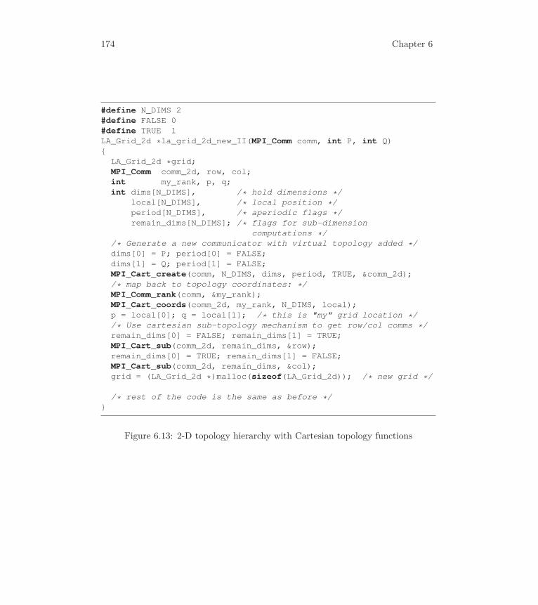
174 Chapter 6
#define N_DIMS 2#define FALSE 0#define TRUE 1LA_Grid_2d *la_grid_2d_new_II(MPI_Comm comm, int P, int Q){
LA_Grid_2d *grid;MPI_Comm comm_2d, row, col;int my_rank, p, q;int dims[N_DIMS], /* hold dimensions */
local[N_DIMS], /* local position */period[N_DIMS], /* aperiodic flags */remain_dims[N_DIMS]; /* flags for sub-dimension
computations *//* Generate a new communicator with virtual topology added */dims[0] = P; period[0] = FALSE;dims[1] = Q; period[1] = FALSE;MPI_Cart_create(comm, N_DIMS, dims, period, TRUE, &comm_2d);/* map back to topology coordinates: */MPI_Comm_rank(comm, &my_rank);MPI_Cart_coords(comm_2d, my_rank, N_DIMS, local);p = local[0]; q = local[1]; /* this is "my" grid location *//* Use cartesian sub-topology mechanism to get row/col comms */remain_dims[0] = FALSE; remain_dims[1] = TRUE;MPI_Cart_sub(comm_2d, remain_dims, &row);remain_dims[0] = TRUE; remain_dims[1] = FALSE;MPI_Cart_sub(comm_2d, remain_dims, &col);grid = (LA_Grid_2d *)malloc(sizeof(LA_Grid_2d)); /* new grid */
/* rest of the code is the same as before */}
Figure 6.13: 2-D topology hierarchy with Cartesian topology functions

Parallel Libraries 175
#define LA_MAPPING_BLINEAR 1#define LA_MAPPING_BSCATTER 2
typedef struct{
int map_type; /* Used for quick comparison of mappings */
void (*mu)(int I, int P, int N, void *extra, int *p, int *i);/* Mapping of I->(p,i) */
void (*mu_inv)(int p, int i, int P, int N, void *extra, int *I);/* Inverse (p,i)->I: */
void (*local_len)(int p, int P, int N, void *extra, int *n);/* # of coefficients mapped to each process: */
void *extra; /* for mapping-specific parameters */} LA_Mapping;
/* some pre-defined mappings ... */extern LA_Mapping *LA_Mapping_Blk_Linear, *LA_Mapping_Blk_Scatter,
*LA_Mapping_Linear, *LA_Mapping_Scatter;
Figure 6.14: Definition of mapping function data structure
typedef struct{
LA_Grid_2d *grid; /* grid on which the distribution is based */LA_Mapping *row; /* row mapping */LA_Mapping *col; /* col mapping */
} LA_Distrib_2d;
Figure 6.15: Definition of distribution data structure
Figure 6.15 illustrates the data structure that encompasses both the logical grid
information and a pair of mappings, which proves sufficient to describe basic linear
algebra.
6.3.2 Vectors and Matrices
Given the logical grids, mappings, and the two-dimension distributions based on
them, we can now turn to distributed data structures for linear algebra.
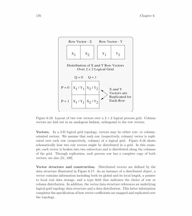
176 Chapter 6
Row Vector - X
Distribution of X and Y Row VectorsOver 2 x 2 Logical Grid
X1 X2
Row Vector - Y
Y1 Y2
X1 / Y1 X2 / Y2
X1 / Y1 X2 / Y2
P = 0
P = 1
Q = 0 Q = 1
X and Y Vectors are Replicated for Each Row
Figure 6.16: Layout of two row vectors over a 2 × 2 logical process grid. Columnvectors are laid out in an analogous fashion, orthogonal to the row vectors.
Vectors. In a 2-D logical grid topology, vectors may be either row- or column-
oriented vectors. We assume that each row (respectively, column) vector is repli-
cated over each row (respectively, column) of a logical grid. Figure 6.16 shows
schematically how two row vectors might be distributed in a grid. In this exam-
ple, each vector is broken into two subvectors and is distributed along the columns
of the grid. Through replication, each process row has a complete copy of both
vectors; see also [51, 109].
Vector structure and construction. Distributed vectors are defined by the
data structure illustrated in Figure 6.17. As an instance of a distributed object, a
vector contains information including both its global and its local length, a pointer
to local real data storage, and a type field that indicates the choice of row or
column distribution. In addition, the vector data structure references an underlying
logical grid topology data structure and a data distribution. This latter information
completes the specification of how vector coefficients are mapped and replicated over
the topology.

Parallel Libraries 177
typedef struct la_local_dvector{
int m; /* local vector length */double *data; /* vector data */
} LA_Local_Dvector;
typedef struct la_dvector{
LA_Local_Dvector v; /* Local vector */int M; /* full length of vector */int type; /* row or column type */LA_Distrib_2d *dis; /* how to map data on grid */
} LA_Dvector;
Figure 6.17: Definition of the distributed vector on the logical grid
Matrices. Matrices on two-dimensional process grids are defined analogously to
vectors, as depicted in Figure 6.18. A matrix is divided into submatrices, each with
a local shape given by m×n. The values of m and n generally differ in each process,
just as the lengths of subvectors differ, in general, in each process. A matrix has
a storage strategy, depending on whether it is row or column major. (The default
constructor we use will make column-major local matrices; this detail remains an
issue for fine optimizations of local memory access.) As with vectors, distributed
matrices refer to an underlying logical process grid and distribution, through which
they acquire the detailed information on topology shape and coefficient mapping.
6.3.3 Components of a Parallel Library
High-quality libraries must provide more than one version of a function that can
perform efficiently over different conditions (we call such a set of methods a poly-
algorithm). For example, we provide multiple versions of the vector sum and inner-
product functions, both with the same sequential complexity. The “strided” version
of these functions has a reduced computational load at the expense of more commu-
nication. Conversely, the “nonstrided” version is computationally more intensive
but requires fewer messages because the algorithm exploits data redundancy; in the
case of the vector sum (with compatibly stored data), no messages are needed at
all. The most efficient function is determined by comparing issues such as message
latency, bandwidth, and floating-point performance, all with reference to the size of
the vector and the logical grid dimensions P , Q. The performance analysis tools we

178 Chapter 6
typedef struct la_local_dmatrix{
int storage_type; /* Storage strategy (row/column-major) */int m, n; /* Local dimensions */double **data; /* The local matrix, as set of pointers */
} LA_Local_Dmatrix;
typedef struct la_dmatrix{
LA_Local_Dmatrix a; /* Local matrix */int M, N; /* Global dimensions of LA_Dmatrix. */LA_Distrib_2d *dis; /* how to map data onto grid */
} LA_Dmatrix;
Figure 6.18: The distributed matrix structure
have described earlier, along with some empirical modeling, can help decide which
function is best for a given case on a real system.
Vector sum. The vector sum is typically a noncommunicating operation provided
the vectors being summed are stored compatibly, that is, corresponding coefficients
appear in the same processes at aligned offsets. This is the simplest of the par-
allel vector operations possible on the distributed vectors. The operation to be
performed is z = αx + βy, where α and β are real scalar constants. Good imple-
mentations handle special cases like α = 0 and β = 1.0 for better performance.
Even better implementations use sequential BLAS (for Basic Linear Algebra Sub-
programs [43, 42, 82]) when local vectors are long enough to make the cost of a
subroutine call less important than the performance gain of an often-optimized
sequential kernel.
Thus, a number of different versions of the vector sum must be available and
must be selected appropriately for different situations. This is where the object-
oriented and object-based approaches to the library design differ. For the object-
oriented case, the user is forced to “commit” to certain operations in order to
pre-evaluate all the data transformations, choices about use of BLAS, and so on.
This approach makes these relatively expensive choices a one-time operation, and
may even encourage further one-time overheads for better performance. The object-
based versions, which are object extensions to the familiar BLAS, have to test for
errors, data layout, and so on each time, making the overhead of general data layouts

Parallel Libraries 179
somewhat higher than the object-oriented versions. These concepts are illustrated
in detail with the code and related documentation described in (Appendix B).
Inner product. The inner product offers a similar set of challenges to those
presented by vector sum; in addition to offering the choices of replicated and non-
replicated work versions, the use or nonuse of underlying BLAS remains. Here, we
illustrate a version of the code that utilizes the object-oriented approach. For this
approach, a “dot product” object is created once, describing the dot-product rela-
tionship between two vectors. Whenever a dot product is needed, (*xy->op)()is performed. The absence of arguments here appears to be a deficiency but is
actually a sign that we have tightly optimized our code! We show the version that
employs sequential BLAS, to remind the reader that we can access efficient local
operations (in the limit of large enough data). See Figures 6.19 and 6.20.
Skew inner product. The skew inner product combines the idea of vector re-
distribution and dot product into a single calculation, when the vectors are not
distributed compatibly at the beginning of the operation. Specifically, it handles
the case where one vector is a “row” vector, in any layout, and the other vector is a
“column” vector. Until now, we have been assuming that the vectors are collinear
(either row or column) and of the same distribution.
Both object-based and object-oriented versions of this call appear in the software
distribution. The nice feature of this routine is that the object-oriented version is
needed to achieve the right computational complexity, because it is essential to
organize the operations in each process once and for all.
Matrix-vector product. To illustrate the use of the vectors together with dense
matrices, we have also included the equivalent object-based and object-oriented
libraries for the dense matrix-vector product. Here the number of choices for data
optimization grows; hence, if the vectors and matrices are distributed incompatibly,
a large number of if statements have to be handled. For the object-oriented
strategy, this is done once and for all. For the object-based approach, lots of
conditional branching gets done with each call.
6.4 The LINPACK Benchmark in MPI
The LINPACK benchmark [5] is a well-known numerical code that is often used
to benchmark computers for floating-point performance. LINPACK itself is an ex-
ample of a successful numerical library, and we briefly discuss some aspects of a

180 Chapter 6
double ddot_stride(LA_Dvector *x, LA_Dvector *y, int *error){
int i, start, stride, m;double local_sum = 0.0, sum, *x_data, *y_data;
if (x->type != y->type) { /* Check for compatible types */
*error = LA_TYPE_ERROR; /* FAILURE */return(0.0);
}
/* Determine the stride based on type */if (x->type == LA_GRID_ROW) {
start = x->dis->grid->p; stride = x->dis->grid->P;}else {
start = x->dis->grid->q; stride = x->dis->grid->Q;}
/* Sum up my part (non-optimized) */m = x->v.m;x_data = &(x->v.data[0]); y_data = &(y->v.data[0]);for (i = start; i < m; i += stride)
local_sum += x_data[i] * y_data[i];
/* Get the sum of all parts */MPI_Allreduce(&local_sum, &sum, 1, MPI_DOUBLE, MPI_SUM,
x->dis->grid->grid_comm);
/* Return result */
*error = MPI_SUCCESS;return(sum);
}
Figure 6.19: Object-based, strided inner (dot) product on distributed vectors, with-out BLAS
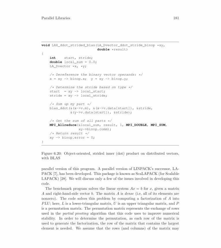
Parallel Libraries 181
void LAX_ddot_strided_blas(LA_Dvector_ddot_stride_binop *xy,double *result)
{int start, stride;double local_sum = 0.0;LA_Dvector *x, *y;
/* Dereference the binary vector operands: */x = xy -> binop.x; y = xy -> binop.y;
/* Determine the stride based on type */start = xy -> local_start;stride = xy -> local_stride;
/* Sum up my part */blas_ddot(&(x->v.m), &(x->v.data[start]), &stride,
&(y->v.data[start]), &stride);
/* Get the sum of all parts */MPI_Allreduce(&local_sum, result, 1, MPI_DOUBLE, MPI_SUM,
xy->binop.comm);/* Return result */xy -> binop.error = 0;
}
Figure 6.20: Object-oriented, strided inner (dot) product on distributed vectors,with BLAS
parallel version of this program. A parallel version of LINPACK’s successor, LA-
PACK [7], has been developed. This package is known as ScaLAPACK (for Scalable
LAPACK) [28]. We will discuss only a few of the issues involved in developing this
code.
The benchmark program solves the linear system Ax = b for x, given a matrix
A and right-hand-side vector b. The matrix A is dense (i.e, all of its elements are
nonzero). The code solves this problem by computing a factorization of A into
PLU ; here, L is a lower-triangular matrix, U is an upper triangular matrix, and P
is a permutation matrix. The permutation matrix represents the exchange of rows
used in the partial pivoting algorithm that this code uses to improve numerical
stability. In order to determine the permutation, as each row of the matrix is
used to generate the factorization, the row of the matrix that contains the largest
element is needed. We assume that the rows (and columns) of the matrix may
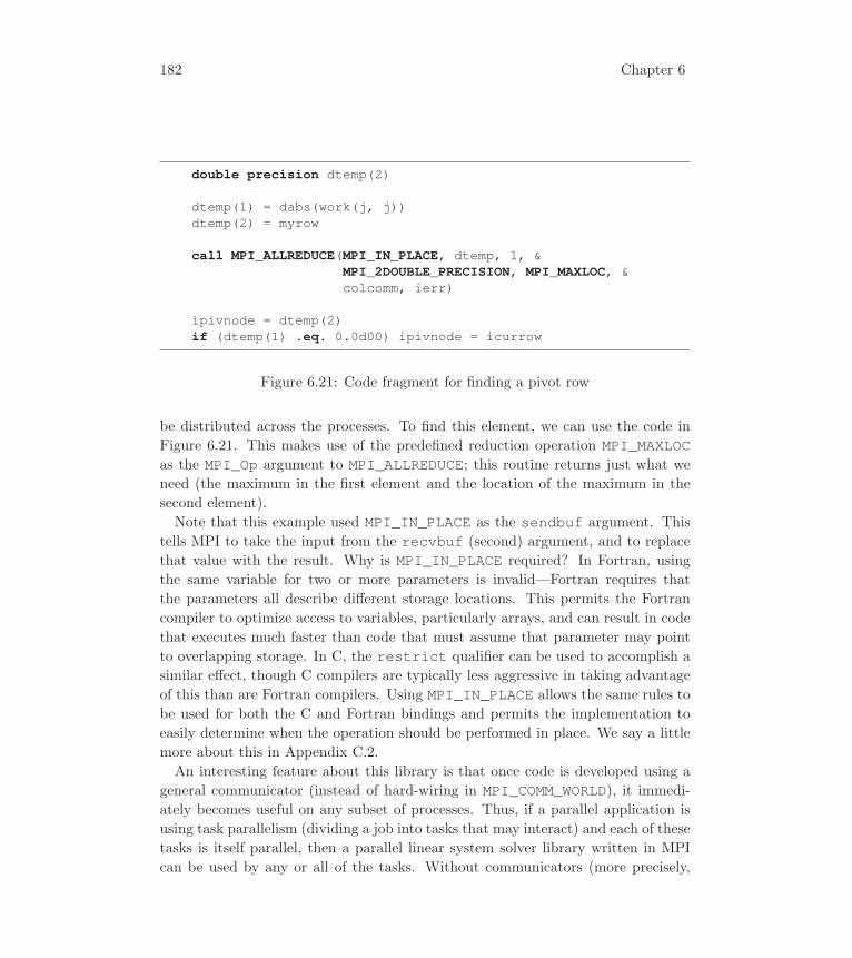
182 Chapter 6
double precision dtemp(2)
dtemp(1) = dabs(work(j, j))dtemp(2) = myrow
call MPI_ALLREDUCE(MPI_IN_PLACE, dtemp, 1, &MPI_2DOUBLE_PRECISION, MPI_MAXLOC, &colcomm, ierr)
ipivnode = dtemp(2)if (dtemp(1) .eq. 0.0d00) ipivnode = icurrow
Figure 6.21: Code fragment for finding a pivot row
be distributed across the processes. To find this element, we can use the code in
Figure 6.21. This makes use of the predefined reduction operation MPI_MAXLOCas the MPI_Op argument to MPI_ALLREDUCE; this routine returns just what we
need (the maximum in the first element and the location of the maximum in the
second element).
Note that this example used MPI_IN_PLACE as the sendbuf argument. This
tells MPI to take the input from the recvbuf (second) argument, and to replace
that value with the result. Why is MPI_IN_PLACE required? In Fortran, using
the same variable for two or more parameters is invalid—Fortran requires that
the parameters all describe different storage locations. This permits the Fortran
compiler to optimize access to variables, particularly arrays, and can result in code
that executes much faster than code that must assume that parameter may point
to overlapping storage. In C, the restrict qualifier can be used to accomplish a
similar effect, though C compilers are typically less aggressive in taking advantage
of this than are Fortran compilers. Using MPI_IN_PLACE allows the same rules to
be used for both the C and Fortran bindings and permits the implementation to
easily determine when the operation should be performed in place. We say a little
more about this in Appendix C.2.
An interesting feature about this library is that once code is developed using a
general communicator (instead of hard-wiring in MPI_COMM_WORLD), it immedi-
ately becomes useful on any subset of processes. Thus, if a parallel application is
using task parallelism (dividing a job into tasks that may interact) and each of these
tasks is itself parallel, then a parallel linear system solver library written in MPI
can be used by any or all of the tasks. Without communicators (more precisely,
Parallel Libraries 183
the group component of the communicator), the library could not be used in this
case.
6.5 Strategies for Library Building
The rest of this chapter concentrates on loosely synchronous parallel libraries. By
loosely synchronous libraries we mean libraries that are essentially single program,
multiple data. They compute on analogous parts of a dataset, however complex or
irregular, and occasionally communicate. Perhaps this communication is collective;
perhaps it is just selective point-to-point transfers. In any event, the number of
messages produced and consumed is well characterized in advance for such libraries;
and most often, both the size and sources for all messages are anticipated at the time
the program is written. That processes may “get ahead” of other processes between
synchronizing communications is the reason for the term loosely synchronous [51].
Also included in this model is the idea that certain processes may send messages
and continue even though their counterpart has failed to complete a receive; for
this purpose, we use MPI send routines that are nonblocking.
Particular strategies are now available to the library writer because of features
in MPI:
• Duplicate communicators for safe communication space when entering calls
to parallel libraries (MPI_Comm_dup, MPI_Comm_create).
• Define distributed structures based on communicators.
• Use MPI-defined virtual topology information to make algorithms easier to
understand (e.g., MPI_Cart_create).
• Augment virtual topology technology as needed (e.g., topology hierarchies,
as in Section 6.3.1).
• Use attributes on communicators (called attribute caching) when adding ad-
ditional collective operations to a communicator (Section 6.2).
• If the library should handle any errors reported by an MPI routine (for exam-
ple, to provide a more application-specific error message), attach a different
error handler to the library’s private communicator (see Section 7.7).
A number of mechanisms used in libraries before MPI to achieve correctness are
no longer necessary and can be safely discarded:
184 Chapter 6
• It is no longer necessary to publish tag usage by the library to avoid tag
conflicts with user code. If the library uses its own communicator, both it
and the user have access to a full range of tags.
• It is no longer necessary to make a parallel library mimic the behavior of a
sequential library by synchronizing at the entry and exit of each parallel call
in order to achieve quiescence. Communicators local to the library ensure
that no library message will be intercepted by user code or vice versa.
• There is no need to restrict the library programming model to nonoverlapping
process group assumptions, since communicators with overlapping groups
pose no particular problem for MPI libraries.
• Many existing libraries work only over “all” processors (processes) of a user’s
allocation. With MPI it is easy to write a library so that it can use whatever
group of processes is specified when it is called.
6.6 Examples of Libraries
One of the hopes of the MPI Forum was that the features in MPI intended for
writing libraries would, in fact, enable the creation of portable libraries, allow-
ing parallel programmers to use ever more powerful constructs in building their
programs.
This hope has indeed been realized, and many large applications make use of
MPI primarily or even entirely through widely used libraries such as FFTW [46],
PETSc [24], ScaLAPACK [28], Trilinos [12], SPRNG [9], and ParMETIS [8]. This
is a very abbreviated list.
In some cases, you may find libraries that are simple ports of libraries written for
previous message-passing systems. These can be useful but, for the reasons given
at the beginning of this chapter, may require care in their use. The most common
limitation is for a library to use MPI_COMM_WORLD for all communication. A
library that uses MPI to properly avoid the possible interference of messages in
the library with ones outside the library will use either MPI_Comm_dup or one of
the other communicator construction routines (such as MPI_Cart_create), anexplicit communicator argument, or MPI_Barrier to separate library messages
from nonlibrary messages. You can often use the Unix command nm to discover
what routines are used in a library. For example, for a static library,
nm /usr/local/lib/libpetsc.a | grep ’U _MPI_’
Parallel Libraries 185
lists all of the MPI routines used in the library libpetsc.a. In many cases, a
similar command will work with shared libraries, though you need to make sure
you apply the command to the library, not to a link that points at the library.
Depending on the exact format of the output of the nm command, the command
nm /usr/local/lib/libpetsc.a | grep -i MPI_ | \awk ’{print $8}’ | sort | uniq
will print a sorted list containing the MPI routines in use (along with other symbols
containing MPI_). If this list contains only a subset of the MPI point-to-point func-
tions (e.g., MPI_Send and MPI_Recv), along with the communicator information
functions MPI_Comm_size and MPI_Comm_rank, then you know that the library
does not use the MPI features for providing communication safety and hence must
be used with care.
6.7 Application: Nuclear Green’s Function Monte Carlo
Our application in this chapter illustrates the use of an MPI-based parallel library
to hide some of the complexity of MPI programming by providing a higher-level
programming model. Sophisticated use of MPI inside the library provides scalability
to the application.
A major goal in nuclear physics is to understand how nuclear binding, stability,
and structure arise from the underlying interactions between individual nucleons.
In the past decade considerable progress has been made in the development of
approaches to the nuclear many-body problem for light nuclei. Physicists from Los
Alamos and Argonne National Laboratories developed the nuclear Green’s Function
Monte Carlo (GFMC) method years ago but recently needed to scale it for execution
on more processors than before, in order to enable nuclear theory computations for
carbon-12, carbon’s most important isotope.
In GFMC calculations the nuclear quantum-mechanical wave function is ex-
pressed as a vector of components describing the state of each nucleon. All the
components are functions of the positions of all of the nucleons. The total numbers
of components in the vectors are 16, 160, 1,792, 21,504, and 267,168 for helium-
4, lithium-6, beryllium-8, boron-10, and carbon-12, respectively. This exponential
growth in components constrains the GFMC method to light nuclei; carbon-12 is
the current limit.
GFMC starts with an approximate wave function and systematically improves it
by damping out “contaminants.” During this process, the nuclear binding energy
computed with the wave function decreases until the remaining contamination is
186 Chapter 6
smaller than the Monte Carlo statistical errors, and the calculation is then stopped.
The improvement (propagation) is done in a series of small steps. Each step requires
a new 3A-dimensional integral (A is the number of nucleons). Thus the whole
GFMC calculation is a huge integral, typically of more than 10,000 dimensions,
which is done by a Monte Carlo method. Various tests indicate that the GFMC
calculations of binding energies have errors of only 1–2%. As Monte Carlo samples
are propagated, they can wander into regions of low importance and be discarded.
Or they can find areas of large importance and will then be multiplied. Hence, the
number of computed samples fluctuates during the calculation.
The problem’s large size demands the use of the largest available computers. The
GFMC program was written in the mid-1990s using MPI, and until 2008 its parallel
structure was largely unchanged. Because of the fluctuating number of samples, the
method depended on the complete evaluation of several (preferably more than 10)
Monte Carlo samples on each MPI rank. These fluctuations also required the work
to be periodically redistributed over the ranks. For carbon-12, only about 15,000
samples are needed, so using the many 10,000s of nodes on forefront computers
such as Argonne’s IBM Blue Gene/P and Blue Gene/Q requires a finer-grained
parallelization in which one sample is computed on many ranks. The ADLB library
was developed to expedite this approach.
The ADLB (Asynchronous Dynamic Load Balancing) library [86] was initially
motivated by the needs of GFMC, but is more general-purpose in its functional-
ity and has been used in a number of other applications as well. (ADLB can be
obtained from [11].) Its basic idea is to create an environment for expressing par-
allel algorithms in a manager-worker framework like that in our early example in
Section 3.6, but utilizing an abstraction that allows a more scalable implementa-
tion. The plan is to replace the explicit manager process by an abstract pool of
work units, which may be implemented in a variety of ways. Instead of sending
“ready” messages and results to the manager and receiving work units to work on
from it, the worker processes put requests and results into the work pool and get
work units from it. PI communication takes place behind the scenes. In one imple-
mentation of ADLB, a (potentially large) number of intercommunicating “ADLB
server” processes manage the work pool. Work unit types and priorities allow one
to construct sophisticated algorithms within this simple application programming
interface. This is done in GFMC.
As the project started, GFMC was running with good efficiency on up to 2,048
MPI ranks. MPI calls were used between the manager rank and worker ranks to
coordinate the workers, direct them to periodically exchange work to maintain load
balancing, and collect and average the Monte Carlo samples. This general structure
Parallel Libraries 187
has been retained when using ADLB, but in addition ADLB calls were inserted to
parcel work (that had all been done on one worker) to multiple workers and then
collect the results. This was typically achieved by replacing a loop that computed
multiple results with two loops: the first loop quickly uses ADLB’s put to deposit
work packages in the pool, and the second gathers the results with ADLB’s get. To
avoid deadlocks, The second loop also accepts work packages of the same type, so
at least one worker will always be available for processing of packages. In this way,
work that was done on only one MPI rank can now be spread across up to 72 ranks
for the case of carbon-12.
A further problem for carbon-12 calculations on the Blue Gene computers is
that there is not enough memory to use each core of a node as a separate MPI
rank. The solution was to adopt a hybrid programming model in which only a few
(perhaps just one) multithreaded ADLB/MPI processes are run on each node of the
machine, making available up to all of each node’s memory. This was accomplished
by using the Fortran version of OpenMP for shared-memory parallelism within a
single address space, which needed to be done only in the computationally intensive
subroutines of the GFMC program. In some cases, however, this approach could
not be used because different iterations of the DO loop accumulate into the same
array element. In such cases an extra dimension was added to the result array so
that each thread can accumulate into its own copy of the array. At the end of
the loop, these copies are added together. OpenMP on the Blue Gene computers
proved to be very efficient; we typically get 90% efficiency. These changes were
independent of using ADLB: even in a pure MPI implementation they would have
been necessary. See 7.5 for a discussion of how to use MPI and OpenMP together.
Calculations of carbon-12 on BG/Q show excellent scaling with increasing num-
ber of nodes. For example, using 8 ranks per node with 6 threads each gives scaling
efficiencies of 85% and 79% for 131,072 and 262,144 ranks, respectively.
Prior to this work, a few calculations of the carbon-12 ground state had been
made with the old GFMC program and merely hundreds of processors. These were
necessarily simplified calculations with significant approximations that produced
questionable results. The combination of BG/P (and now BG/Q) and the ADLB
version of the program has completely changed this situation. We first made one
very large calculation of the carbon-12 ground state using our best interaction
model and none of the previously necessary approximations. This calculation was
made with an extra large number of Monte Carlo samples to allow various tests
of convergence of several aspects of the GFMC method. These tests showed that
our standard GFMC calculation parameters for lighter nuclei were also good for
carbon-12.

188 Chapter 6
The results of the calculation were also encouraging. The computed binding en-
ergy of carbon-12 is 93.2 MeV, with a Monte Carlo statistical error of 0.6 MeV.
Based on the convergence tests and our experience with GFMC, we estimate the sys-
tematic errors at approximately 1 MeV. Thus, this result is in excellent agreement
with the experimental binding energy of 92.16 MeV.

7 Other Features of MPI
This chapter describes the more advanced routines from the MPI standard that
have not arisen in the discussion so far. We use the opportunity to introduce
several interesting example programs.
7.1 Working with Global Data
Throughout this book we have been concentrating on the message-passing compu-
tational model. Some applications are more naturally written for a global memory
model in which all of the parallel machine’s memory is directly available to each
process. In this section we discuss what is necessary in order to provide the basic
functionality of the global-memory model in a distributed-memory environment,
and what MPI routines might be used in doing so. The example provided here is
just one way in which this may be accomplished in MPI; others include one-sided
memory access, described in Using Advanced MPI [55], and the use of threads as
message agents. We call this global data rather than shared memory because we
will still require the use of MPI routine calls to access and update the global data,
unlike shared memory models where simple reference and assignment are used to
access and update values. What’s important here is the style of access—in the
cases we’ll describe, there is data in which all processes are interested, unlike most
of our previous examples where just a few processes exchanged any particular piece
of information. MPI also provides a different programming model, the one-sided
communication, that is well-suited to these sorts of programs. The one-sided model
is covered in Using Advanced MPI.
7.1.1 Shared Memory, Global Data, and Distributed Memory
The essential feature of the message-passing model is that at least two processes
are involved in every communication; send and receive operations must be paired.
The essential feature of a shared-memory model is that any process can access all
the memory in the machine. On a distributed-memory architecture, where each
memory address is local to a specific processor, this means that each process must
be able to access the local memory of other processes, without any particular action
on the part of the process whose local memory is being read or written to.
In a sense, then, every processor (CPU plus memory) must be host to two different
functions: a compute process that does the main work, and a data server process
that provides the other processes in the computation access to that processor’s
memory (see Figure 7.1). These two processes need not be separate MPI processes.

190 Chapter 7
�����������
������ �����������
����������
����
Figure 7.1: Sharing distributed memory
In many cases the machine’s operating system or message-passing software will not
permit it, and in other cases the overhead of switching between the two processes
is prohibitive.
Several approaches exist, depending on what level of extension to the message-
passing model is offered by the underlying system. One approach is to use a separate
thread to handle the data management requests. A more direct approach, called
one-sided or remote memory access, is available in MPI and is discussed in Using
Advanced MPI [55]. We use this example to illustrate the use of two-sided message
passing to provide a data service—in this case, a simple counter. The same ideas
can be used to provide more complex services, including ones that require more
complex computation than a simple increment.
7.1.2 A Counter Example
We begin with the simplest possible case: simulating a single shared-memory lo-
cation. Having a single “shared” variable that can be updated atomically by any
process is surprisingly useful. In a true shared-memory environment, the counter
is read and updated by normal memory operations, but the updating must be pro-
tected by a lock of some kind. In the message-passing environment, no lock is
needed because only one process is actually updating the memory location. Hence,
one easy way to implement the shared counter with MPI is to give one MPI pro-

Other Features of MPI 191
cess the job of holding the counter and servicing requests to retrieve and update
its value. To make things particularly straightforward, let us suppose we wish to
implement a function NXTVAL that returns the value of a built-in counter that is
initialized to 0 at startup. Each retrieval of its value increments the value by one.
With many processes calling NXTVAL, it is guaranteed that no two will ever retrieve
the same value and that all values of the counter will handed out consecutively, with
no value being skipped.
We dedicate one process1 to being the “server” for this variable. It can be set
up much the same way in which we established the server for random numbers
in Chapter 3. Let us encapsulate the counter by defining of set of three routines
to manage it for the MPE library: MPE_Counter_create, MPE_Counter_-free, and MPE_Counter_nxtval. MPE_Counter_create will be a collective
operation (must be called by all processes in a given communicator); it will split
off one process of the communicator’s group to hold the counter and return two
new communicators. One communicator, counter_comm, will be used in calls to
MPE_Counter_nxtval; the other, smaller_comm, will be used by the remain-
ing processes for the main computation. MPE_Counter_free cleans up these
communicators and ends the server process function, terminating its original call
to MPI_Counter_create. This strategy relies on the fact that MPI, unlike many
other systems, supports collective and point-to-point operations on communicators
based on arbitrary subgroups of processes. Thus, the communicator smaller_-comm is just as capable as the communicator passed to MPI_Counter_create,except that it has one less process available.
This client-server computation is easy enough that we can include all the nec-
essary code here. MPE_Counter_create is shown in Figure 7.2, including the
handling of an unexpected tag (signifying an error in our program) that uses MPI_-Abort to cause the program to exit (see Section 7.7.4). MPE_Counter_nxtvalis shown in Figure 7.3. MPE_Counter_free is shown in Figure 7.4; it is also a
collective operation. The process with rank zero in the counter’s communicator
sends a message to the counter process to make it call MPE_Counter_free as
well.
We use MPI_Comm_split to create the smaller communicator smaller_comm.We do this by using the special value MPI_UNDEFINED as the value of color for
the process that is the counter process and is not in the smaller_comm commu-
nicator. For this process, MPI_Comm_split returns a value of MPI_COMM_NULL.
1In some MPI implementations, multiple MPI processes per processor are allowed. The MPIstandard neither requires nor prohibits it. This example makes the most sense in such an envi-ronment; otherwise, one processor is idle most of the time waiting for counter requests.
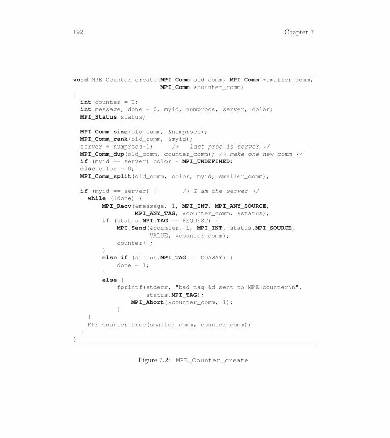
192 Chapter 7
void MPE_Counter_create(MPI_Comm old_comm, MPI_Comm *smaller_comm,MPI_Comm *counter_comm)
{int counter = 0;int message, done = 0, myid, numprocs, server, color;MPI_Status status;
MPI_Comm_size(old_comm, &numprocs);MPI_Comm_rank(old_comm, &myid);server = numprocs-1; /* last proc is server */MPI_Comm_dup(old_comm, counter_comm); /* make one new comm */if (myid == server) color = MPI_UNDEFINED;else color = 0;MPI_Comm_split(old_comm, color, myid, smaller_comm);
if (myid == server) { /* I am the server */while (!done) {
MPI_Recv(&message, 1, MPI_INT, MPI_ANY_SOURCE,MPI_ANY_TAG, *counter_comm, &status);
if (status.MPI_TAG == REQUEST) {MPI_Send(&counter, 1, MPI_INT, status.MPI_SOURCE,
VALUE, *counter_comm);counter++;
}else if (status.MPI_TAG == GOAWAY) {
done = 1;}else {
fprintf(stderr, "bad tag %d sent to MPE counter\n",status.MPI_TAG);
MPI_Abort(*counter_comm, 1);}
}MPE_Counter_free(smaller_comm, counter_comm);
}}
Figure 7.2: MPE_Counter_create

Other Features of MPI 193
int MPE_Counter_nxtval(MPI_Comm counter_comm, int *value){
int server,numprocs;MPI_Comm_size(counter_comm, &numprocs);server = numprocs-1;MPI_Send(NULL, 0, MPI_INT, server, REQUEST, counter_comm);MPI_Recv(value, 1, MPI_INT, server, VALUE, counter_comm,
MPI_STATUS_IGNORE);return 0;
}
Figure 7.3: MPE_Counter_nxtval
int MPE_Counter_free(MPI_Comm *smaller_comm,MPI_Comm *counter_comm)
{int myid, numprocs;MPI_Comm_rank(*counter_comm, &myid);MPI_Comm_size(*counter_comm, &numprocs);/* Make sure that all requests have been serviced */if (myid == 0)
MPI_Send(NULL, 0, MPI_INT, numprocs-1, GOAWAY,
*counter_comm);MPI_Comm_free(counter_comm);if (*smaller_comm != MPI_COMM_NULL) {
MPI_Comm_free(smaller_comm);}return 0;
}
Figure 7.4: Code for MPE_Counter_free
All other processes are placed in the new communicator; because we used myid as
the key argument, they are ordered in smaller_comm the same as in old_comm.
7.1.3 The Shared Counter Using Polling Instead of an Extra Process
The disadvantage of the implementation we have just described is, of course, that
one process is “wasted” minding the counter when it could perhaps be used in
computation. To get around this disadvantage, this process must do useful work
and manage the counter simultaneously. One way to do so within the restrictions
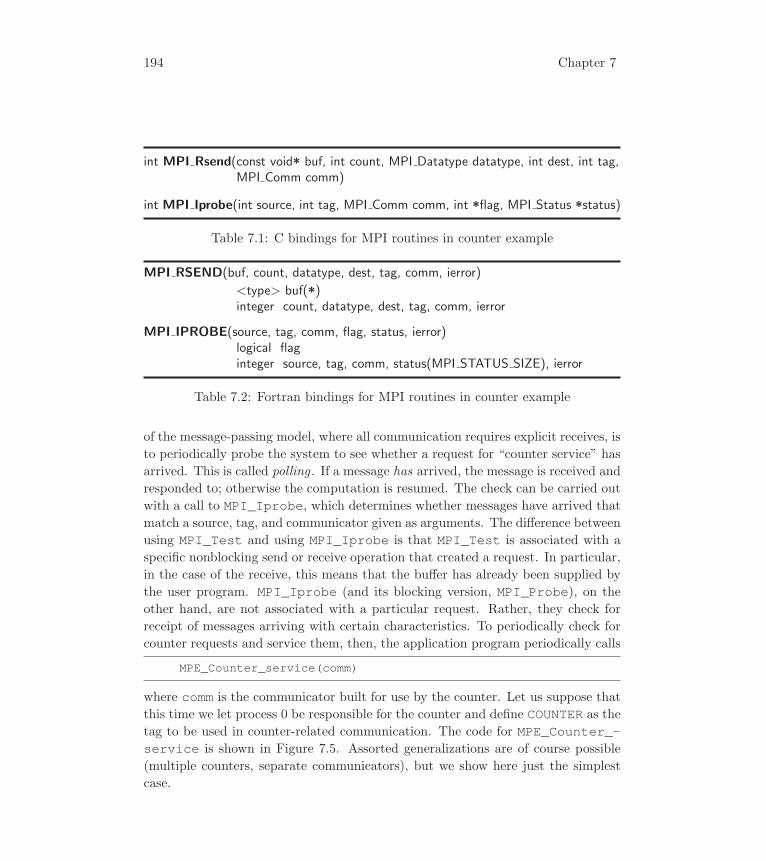
194 Chapter 7
int MPI Rsend(const void* buf, int count, MPI Datatype datatype, int dest, int tag,MPI Comm comm)
int MPI Iprobe(int source, int tag, MPI Comm comm, int *flag, MPI Status *status)
Table 7.1: C bindings for MPI routines in counter example
MPI RSEND(buf, count, datatype, dest, tag, comm, ierror)
<type> buf(*)integer count, datatype, dest, tag, comm, ierror
MPI IPROBE(source, tag, comm, flag, status, ierror)logical flaginteger source, tag, comm, status(MPI STATUS SIZE), ierror
Table 7.2: Fortran bindings for MPI routines in counter example
of the message-passing model, where all communication requires explicit receives, is
to periodically probe the system to see whether a request for “counter service” has
arrived. This is called polling . If a message has arrived, the message is received and
responded to; otherwise the computation is resumed. The check can be carried out
with a call to MPI_Iprobe, which determines whether messages have arrived that
match a source, tag, and communicator given as arguments. The difference between
using MPI_Test and using MPI_Iprobe is that MPI_Test is associated with a
specific nonblocking send or receive operation that created a request. In particular,
in the case of the receive, this means that the buffer has already been supplied by
the user program. MPI_Iprobe (and its blocking version, MPI_Probe), on the
other hand, are not associated with a particular request. Rather, they check for
receipt of messages arriving with certain characteristics. To periodically check for
counter requests and service them, then, the application program periodically calls
MPE_Counter_service(comm)
where comm is the communicator built for use by the counter. Let us suppose that
this time we let process 0 be responsible for the counter and define COUNTER as the
tag to be used in counter-related communication. The code for MPE_Counter_-service is shown in Figure 7.5. Assorted generalizations are of course possible
(multiple counters, separate communicators), but we show here just the simplest
case.

Other Features of MPI 195
void MPE_Counter_service(MPI_Comm comm){
static int counter = 0;int requester, flag;MPI_Status status;/* Process all pending messages */do {
MPI_Iprobe(MPI_ANY_SOURCE, COUNTER, comm, &flag, &status);if (flag) {
requester = status.MPI_SOURCE;MPI_Recv(MPI_BOTTOM, 0, MPI_INT, requester, COUNTER,
comm, MPI_STATUS_IGNORE);counter++;MPI_Send(&counter, 1, MPI_INT, requester,
COUNTER, comm);}
} while (flag);}
Figure 7.5: MPE_Counter_service
The programmer is responsible for seeing that this routine gets called often
enough by the server process to service requests. One way to do this might be
to use the profiling interface described in Section 7.6 to intercept MPI calls and
probe for messages. Another way is to create a separate thread that does noth-
ing but call MPE_Counter_service. Ensuring that the communication system
responds to requests is a deep subject, often discussed under the general name
of ensuring progress or just progress. The MPI library itself must decide how to
respond to incoming data, and the specific choice made by the implementors is
unlikely to be optimal for all applications. Thus, you may see applications call-
ing MPI_Iprobe or MPI_Test “to ensure progress”. In this case, they are doing
for the MPI implementation what calling MPE_Counter_service does for the
nxtval service.
The requests for the counter service themselves are made with
MPI_Send(NULL, 0, MPI_INT, 0, COUNTER, comm);MPI_Recv(&val, 1, MPI_INT, 0, COUNTER, comm, MPI_STATUS_IGNORE);
Note the explicit known server and tag. The count field in the send is 0 because
no data is associated with the request; the tag is enough. Note that we also could
have used MPI_Sendrecv here.
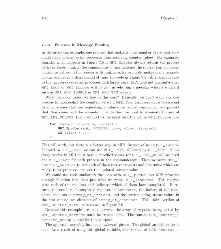
196 Chapter 7
7.1.4 Fairness in Message Passing
In the preceding example, one process that makes a large number of requests very
quickly can prevent other processes from receiving counter values. For example,
consider what happens in Figure 7.5 if MPI_Iprobe always returns the process
with the lowest rank in the communicator that matches the source, tag, and com-
municator values. If the process with rank zero, for example, makes many requests
for the counter in a short period of time, the code in Figure 7.5 will give preference
to that process over other processes with larger rank. MPI does not guarantee that
MPI_Recv or MPI_Iprobe will be fair in selecting a message when a wildcard
such as MPI_ANY_SOURCE or MPI_ANY_TAG is used.
What behavior would we like in this case? Basically, we don’t want any one
process to monopolize the counter; we want MPE_Counter_service to respond
to all processes that are requesting a value once before responding to a process
that “has come back for seconds.” To do this, we need to eliminate the use of
MPI_ANY_SOURCE. But if we do this, we must turn the call to MPI_Iprobe into
for (rank=0; rank<size; rank++) {MPI_Iprobe(rank, COUNTER, comm, &flag, &status);if (flag) { ... }
}
This will work, but there is a better way in MPI. Instead of using MPI_Iprobefollowed by MPI_Recv, we can use MPI_Irecv, followed by MPI_Test. Since
every receive in MPI must have a specified source (or MPI_PROC_NULL), we need
one MPI_Irecv for each process in the communicator. Then we want MPE_-Counter_service to test each of these receive requests and determine which are
ready; those processes are sent the updated counter value.
We could use code similar to the loop with MPI_Iprobe, but MPI provides
a single function that does just what we want: MPI_Testsome. This routine
tests each of the requests and indicates which of them have completed. It re-
turns the number of completed requests in outcount, the indices of the com-
pleted requests in array_of_indices, and the corresponding status values in
the first outcount elements of array_of_statuses. This “fair” version of
MPE_Counter_service is shown in Figure 7.6.
Because this example uses MPI_Irecv, the array of requests being tested by
MPE_Counter_service must be created first. The routine MPE_Counter_-service_setup is used for that purpose.
The approach arguably has some awkward pieces. The global variable reqs is
one. As a result of using this global variable, this version of MPE_Counter_-
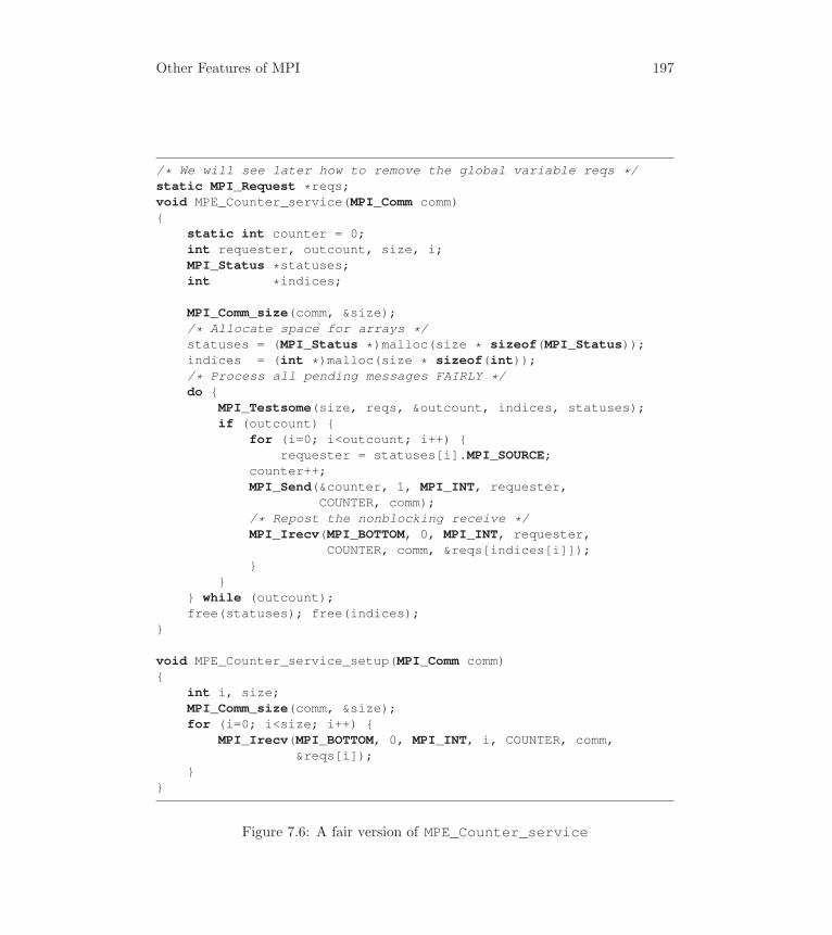
Other Features of MPI 197
/* We will see later how to remove the global variable reqs */static MPI_Request *reqs;void MPE_Counter_service(MPI_Comm comm){
static int counter = 0;int requester, outcount, size, i;MPI_Status *statuses;int *indices;
MPI_Comm_size(comm, &size);/* Allocate space for arrays */statuses = (MPI_Status *)malloc(size * sizeof(MPI_Status));indices = (int *)malloc(size * sizeof(int));/* Process all pending messages FAIRLY */do {
MPI_Testsome(size, reqs, &outcount, indices, statuses);if (outcount) {
for (i=0; i<outcount; i++) {requester = statuses[i].MPI_SOURCE;
counter++;MPI_Send(&counter, 1, MPI_INT, requester,
COUNTER, comm);/* Repost the nonblocking receive */MPI_Irecv(MPI_BOTTOM, 0, MPI_INT, requester,
COUNTER, comm, &reqs[indices[i]]);}
}} while (outcount);free(statuses); free(indices);
}
void MPE_Counter_service_setup(MPI_Comm comm){
int i, size;MPI_Comm_size(comm, &size);for (i=0; i<size; i++) {
MPI_Irecv(MPI_BOTTOM, 0, MPI_INT, i, COUNTER, comm,&reqs[i]);
}}
Figure 7.6: A fair version of MPE_Counter_service

198 Chapter 7
service can be used with only one communicator at a time. In addition, the
MPE_Counter_service routine must use malloc and free to provide tempo-
rary arrays for MPI_Testsome. This is a place where attributes attached to the
communicator, using the approach from Section 6.2, are a natural and powerful
way to improve the usability of a library routine.
Another awkward issue is all of the MPI requests created by the call to MPI_-Irecv. In this code, a receive is always preposted so that it is ready for an
incoming messages. But what happens when we’re done with the counter? Each
process will be one request for every process in the communicator. What we need
is a way to tell MPI to discard these receive requests. MPI provides MPI_Cancelfor just this purpose. For a receive request, cancellation checks to see if the receive
request has been satisfied. If not, then the request is removed from the queue of
posted receives2; thus, once a receive request is canceled, it cannot be matched by a
subsequent send. In this case, the cancel succeeds. However, it is possible that the
request has already been matched by a send. In that case, the cancel attempt will
fail. In both cases, it is necessary to complete the request with any of the request
completion routines. To determine if the cancellation was successful, the routine
MPI_Test_cancelled should be called. A typical use of MPI_Cancel is
...MPI_Cancel(&req);MPI_Wait(&req,&status);MPI_Test_cancelled(&status,&flag);if (flag) {
... message was successfully canceled}
Note that the MPI_Wait call is guaranteed to complete—either the message was
successfully canceled, or the message has been matched, and the message will be
delivered. The bindings for these routines are shown in Tables 7.3 and 7.4.
The approach used by MPI to provide fairness in message passing is very sim-
ilar to the approach used in Unix to provide fairness in handling read and write
operations with file descriptors. See Chapter 9 for details.
7.1.5 Exploiting Request-Response Message Patterns
In the preceding two sections, “shared memory” has consisted of a single value held
by a single process. At this point, however, it is not difficult to see how to generalize
2This is a conceptual queue—different MPI implementations make use different strategies, butthey will all act as if there is a queue of posted receives.
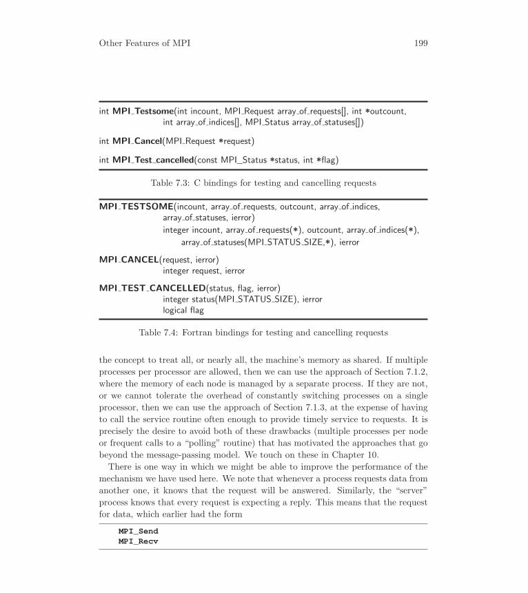
Other Features of MPI 199
int MPI Testsome(int incount, MPI Request array of requests[], int *outcount,int array of indices[], MPI Status array of statuses[])
int MPI Cancel(MPI Request *request)
int MPI Test cancelled(const MPI_Status *status, int *flag)
Table 7.3: C bindings for testing and cancelling requests
MPI TESTSOME(incount, array of requests, outcount, array of indices,array of statuses, ierror)
integer incount, array of requests(*), outcount, array of indices(*),
array of statuses(MPI STATUS SIZE,*), ierror
MPI CANCEL(request, ierror)integer request, ierror
MPI TEST CANCELLED(status, flag, ierror)integer status(MPI STATUS SIZE), ierrorlogical flag
Table 7.4: Fortran bindings for testing and cancelling requests
the concept to treat all, or nearly all, the machine’s memory as shared. If multiple
processes per processor are allowed, then we can use the approach of Section 7.1.2,
where the memory of each node is managed by a separate process. If they are not,
or we cannot tolerate the overhead of constantly switching processes on a single
processor, then we can use the approach of Section 7.1.3, at the expense of having
to call the service routine often enough to provide timely service to requests. It is
precisely the desire to avoid both of these drawbacks (multiple processes per node
or frequent calls to a “polling” routine) that has motivated the approaches that go
beyond the message-passing model. We touch on these in Chapter 10.
There is one way in which we might be able to improve the performance of the
mechanism we have used here. We note that whenever a process requests data from
another one, it knows that the request will be answered. Similarly, the “server”
process knows that every request is expecting a reply. This means that the request
for data, which earlier had the form
MPI_SendMPI_Recv

200 Chapter 7
can be recoded as
MPI_IrecvMPI_SendMPI_Wait
On some architectures, particularly more loosely coupled systems that use networks
to communicate data between processes, the protocol that takes place between
sending and receiving processes can be greatly simplified if the sending process can
assume that the matching receive has already been posted. The reason the protocol
can be simpler is that if the sending side knows that a buffer has been supplied (this
is the main function of MPI_Irecv), any negotiations between the processes over
buffer space can be bypassed. In fact, some network approaches, such as remote
direct memory access (RDMA) that are supported by networks such as InfiniBand,
require that receive buffers exist, and require additional coding and message traffic
to ensure that these buffers are available. MPI provides a special form of the send
for this situation. If the sender is assured that the receive has already been posted,
then it may use MPI_Rsend. (The “R” is for “receiver ready,”; the MPI standard
calls this kind of send a “ready send”.) The MPI implementation may treat this as
a normal send (the semantics are the same as those of MPI_Send) but is allowedto optimize the protocol if it can. If the corresponding receive is not posted, then
this is treated as a programmer error, and MPI’s behavior is undefined in this case.
Because it is important when using MPI_Rsend to consider both the sending and
receiving side, we show a sketch of the code for the two processes below.
Requester ServerMPI_IrecvMPI_Send MPI_Recv
MPI_RsendMPI_Wait
A further refinement is to use MPI_Rsend in both the requester and the server.
Note that MPI_Rsend should be used only when it is known that the receive is
already issued. For the most part, message-passing programming purposely allows
few opportunities for writing code whose correct execution depends on the exact
timing and order of events, but MPI_Rsend makes it possible to write code that
is formally incorrect (because the program does not guarantee that MPI_Rsendis never called unless the matching MPI_Recv has already been issued) but that
runs correctly most of the time. This means that MPI_Rsend should be used
only when it can be shown to improve performance, and only with great care. In
addition, few implementations currently exploit the opportunities offered to an MPI
Other Features of MPI 201
implementation, though at least one does, and performance tests have shown some
benefits to using it on that implementation of MPI.
7.2 Advanced Collective Operations
In the book so far, we have introduced new collective operations of MPI as a
consequence of trying to create a parallel algorithm, code, or library. At this
stage, a few routines remain that we haven’t needed in our palette of examples.
Since these routines are important, and may be just what is needed to get the job
done, we present them here all at once. In this book, we restrict ourselves to the
collective routines defined in MPI-1 and MPI-2. MPI-3 added two more categories
of collectives: nonblocking and neighborhood collectives. These are described in
the companion volume, Using Advanced MPI [55].
7.2.1 Data Movement
MPI provides many operations for collective data movement. We have already
seen MPI_Bcast and the gather routines. In addition to these, MPI provides
the opposite of gather, called scatter (MPI_Scatter and MPI_Scatterv), and a
kind of “all scatter” called alltoall (MPI_Alltoall and MPI_Alltoallv). MPI-
2 introduced an additional variation of MPI_Alltoallv called MPI_Alltoallw.These are illustrated in Figure 7.7.
7.2.2 Collective Computation
We have already seen several collective computation routines; MPI_Reduce per-
forms a reduction of data from each process onto the specified root process. We
have seen the use of MPI_SUM as the operation given to MPI_Reduce to sum up
entries from all of the processes in a communicator. MPI provides a number of
additional operations, shown in Table 7.5, that can be used with any of the col-
lective computation routines. Most of these are self-explanatory. The last two,
MPI_MAXLOC and MPI_MINLOC, are similar to MPI_MAX and MPI_MIN except
that they also return the rank of the process where the maximum or minimum was
found (if several processes have the maximum or minimum, the rank of the first one
is returned). The datatype that is used for MPI_MAXLOC and MPI_MINLOC con-
tains both the value and the rank; see the MPI standard or the implementation’s
man pages on MPI_MAXLOC and MPI_MINLOC for more details.
Several additional predefined operations were introduced in MPI-2 that are in-
tended for use with the one-sided communication functions. These include MPI_-
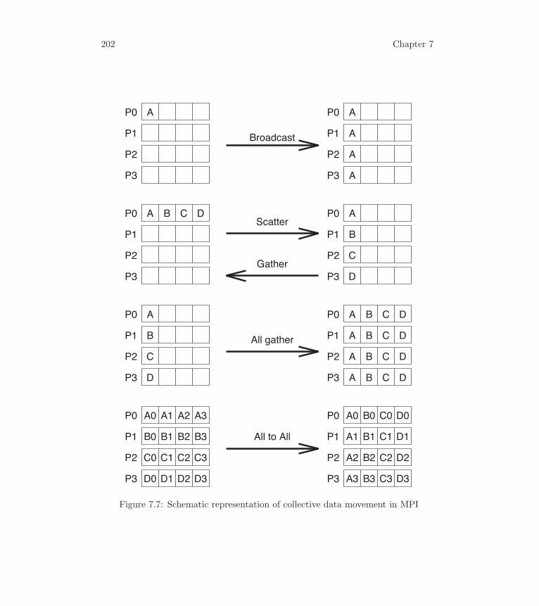
202 Chapter 7
P0
P1
P2
P3
P0
P1
P2
P3
P0
P1
P2
P3
P0
P1
P2
P3
P0
P1
P2
P3
P0
P1
P2
P3
P0
P1
P2
P3
P0
P1
P2
P3
A A
A
A
A
A B C D A
B
C
D
A
B
C
D
A B C D
A B C D
A B C D
A B C D
A0 A1 A2 A3
B0 B1 B2 B3
C0 C1 C2 C3
D0 D1 D2 D3
A0 B0 C0 D0
A1 B1 C1 D1
A2 B2 C2 D2
A3 B3 C3 D3
All to All
All gather
Scatter
Gather
Broadcast
Figure 7.7: Schematic representation of collective data movement in MPI
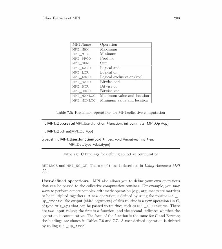
Other Features of MPI 203
MPI Name OperationMPI_MAX MaximumMPI_MIN MinimumMPI_PROD ProductMPI_SUM SumMPI_LAND Logical andMPI_LOR Logical orMPI_LXOR Logical exclusive or (xor)MPI_BAND Bitwise andMPI_BOR Bitwise orMPI_BXOR Bitwise xorMPI_MAXLOC Maximum value and locationMPI_MINLOC Minimum value and location
Table 7.5: Predefined operations for MPI collective computation
int MPI Op create(MPI User function *function, int commute, MPI Op *op)
int MPI Op free(MPI Op *op)
typedef int MPI User function(void *invec, void *inoutvec, int *len,
MPI Datatype *datatype)
Table 7.6: C bindings for defining collective computation
REPLACE and MPI_NO_OP. The use of these is described in Using Advanced MPI
[55].
User-defined operations. MPI also allows you to define your own operations
that can be passed to the collective computation routines. For example, you may
want to perform a more complex arithmetic operation (e.g., arguments are matrices
to be multiplied together). A new operation is defined by using the routine MPI_-Op_create; the output (third argument) of this routine is a new operation (in C,
of type MPI_Op) that can be passed to routines such as MPI_Allreduce. Thereare two input values; the first is a function, and the second indicates whether the
operation is commutative. The form of the function is the same for C and Fortran;
the bindings are shown in Tables 7.6 and 7.7. A user-defined operation is deleted
by calling MPI_Op_free.
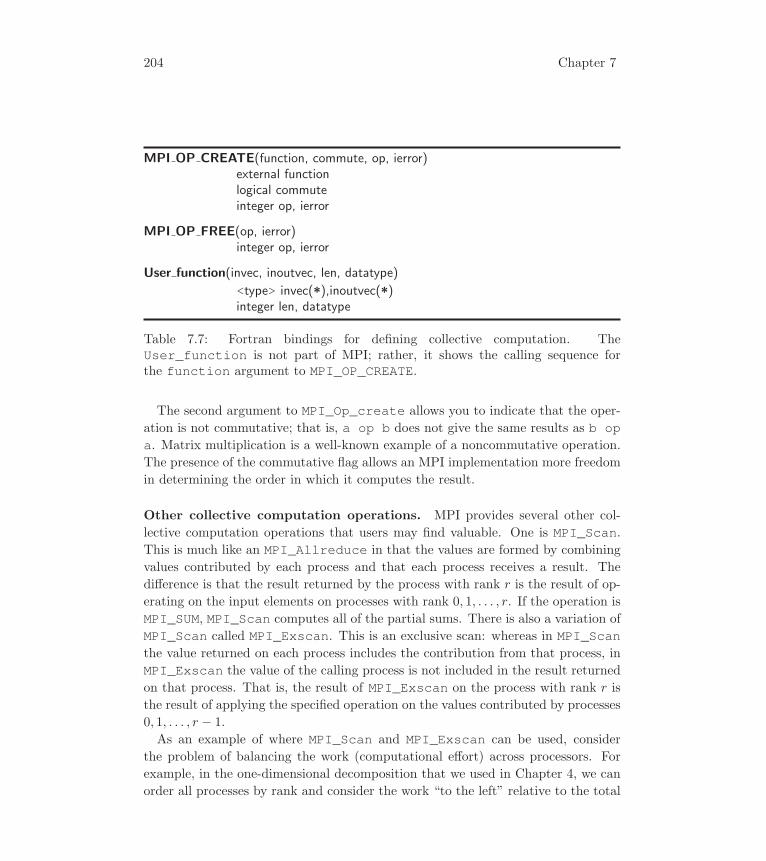
204 Chapter 7
MPI OP CREATE(function, commute, op, ierror)external functionlogical commuteinteger op, ierror
MPI OP FREE(op, ierror)integer op, ierror
User function(invec, inoutvec, len, datatype)
<type> invec(*),inoutvec(*)integer len, datatype
Table 7.7: Fortran bindings for defining collective computation. TheUser_function is not part of MPI; rather, it shows the calling sequence forthe function argument to MPI_OP_CREATE.
The second argument to MPI_Op_create allows you to indicate that the oper-
ation is not commutative; that is, a op b does not give the same results as b opa. Matrix multiplication is a well-known example of a noncommutative operation.
The presence of the commutative flag allows an MPI implementation more freedom
in determining the order in which it computes the result.
Other collective computation operations. MPI provides several other col-
lective computation operations that users may find valuable. One is MPI_Scan.This is much like an MPI_Allreduce in that the values are formed by combining
values contributed by each process and that each process receives a result. The
difference is that the result returned by the process with rank r is the result of op-
erating on the input elements on processes with rank 0, 1, . . . , r. If the operation is
MPI_SUM, MPI_Scan computes all of the partial sums. There is also a variation of
MPI_Scan called MPI_Exscan. This is an exclusive scan: whereas in MPI_Scanthe value returned on each process includes the contribution from that process, in
MPI_Exscan the value of the calling process is not included in the result returned
on that process. That is, the result of MPI_Exscan on the process with rank r is
the result of applying the specified operation on the values contributed by processes
0, 1, . . . , r − 1.
As an example of where MPI_Scan and MPI_Exscan can be used, consider
the problem of balancing the work (computational effort) across processors. For
example, in the one-dimensional decomposition that we used in Chapter 4, we can
order all processes by rank and consider the work “to the left” relative to the total

Other Features of MPI 205
work. That is, if the work is evenly distributed, each process will find that the sum
of work to the left, not counting the current process, will be rank * total_work/ nprocs. The following code provides a simple sketch:
t1 = MPI_Wtime();... work ...my_time = MPI_Wtime() - t1;MPI_Scan(&my_time, &time_to_me, 1, MPI_DOUBLE,
MPI_SUM, MPI_COMM_WORLD);total_work = time_to_me; // Only for the last processMPI_Bcast(&total_work, 1, MPI_DOUBLE, nprocs-1, MPI_COMM_WORLD);fair_share = (rank + 1) * total_work / nprocs;if (fair_share > time_to_me + EPS) {
... shift work to rank-1}else if (fair_share < time_to_me - EPS) {
... shift work to rank+1}
With MPI_Exscan, the fair_share term would use rank instead of rank +1.The other collective computation routine is MPI_Reduce_scatter. The effect
of this routine is to combine an MPI_Reduce and a MPI_Scatterv. This routinecan be used to perform multiple MPI_Reduce operations concurrently and, in a
sophisticated MPI implementation, can run faster than using MPI_Reduce and
MPI_Scatterv. To see how this can be used, consider the problem of forming a
matrix-vector product where the matrix and the vector are distributed across the
processes. The vectors are distributed as follows: each process has some contigu-
ous section of the vector, and these sections are in rank order. That is, process
zero has the first chunk of values, process one the next chunk, and so on. More
precisely, if the full vector is of size n and there are nprocs processes, then pro-
cess zero has elements (starting from 1) 1:n/nprocs, the second has elements
n/nprocs+1:2n/nprocs, and so on (we are assuming that nprocs divides nhere for simplicity).
The matrix is distributed across the processes by columns: the process with
rank zero has columns 1:n/nprocs and all of the rows, process one has columns
n/nprocs+1:2n/nprocs, and so on. The distribution of the matrix and the
vectors across the processes is shown in Figure 7.8.
We want to form the matrix-vector product y = Ax. Let Ai denote the part of
the matrix A that is on process i, and let xi denote the part of the vector x that
is on process i. Because we have distributed A across the processes by column, we
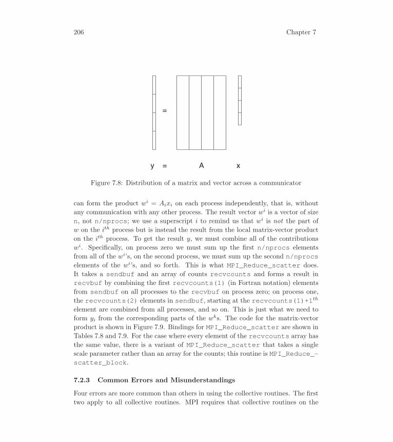
206 Chapter 7
=
y = A x
Figure 7.8: Distribution of a matrix and vector across a communicator
can form the product wi = Aixi on each process independently, that is, without
any communication with any other process. The result vector wi is a vector of size
n, not n/nprocs; we use a superscript i to remind us that wi is not the part of
w on the ith process but is instead the result from the local matrix-vector product
on the ith process. To get the result y, we must combine all of the contributions
wi. Specifically, on process zero we must sum up the first n/nprocs elements
from all of the wi’s, on the second process, we must sum up the second n/nprocselements of the wi’s, and so forth. This is what MPI_Reduce_scatter does.
It takes a sendbuf and an array of counts recvcounts and forms a result in
recvbuf by combining the first recvcounts(1) (in Fortran notation) elements
from sendbuf on all processes to the recvbuf on process zero; on process one,
the recvcounts(2) elements in sendbuf, starting at the recvcounts(1)+1th
element are combined from all processes, and so on. This is just what we need to
form yi from the corresponding parts of the wks. The code for the matrix-vector
product is shown in Figure 7.9. Bindings for MPI_Reduce_scatter are shown in
Tables 7.8 and 7.9. For the case where every element of the recvcounts array has
the same value, there is a variant of MPI_Reduce_scatter that takes a single
scale parameter rather than an array for the counts; this routine is MPI_Reduce_-scatter_block.
7.2.3 Common Errors and Misunderstandings
Four errors are more common than others in using the collective routines. The first
two apply to all collective routines. MPI requires that collective routines on the
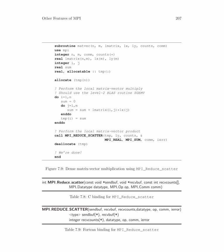
Other Features of MPI 207
subroutine matvec(n, m, lmatrix, lx, ly, counts, comm)use mpiinteger n, m, comm, counts(*)real lmatrix(n,m), lx(m), ly(m)integer i, jreal sumreal, allocatable :: tmp(:)
allocate (tmp(n))
! Perform the local matrix-vector multiply! Should use the level-2 BLAS routine SGEMVdo i=1,n
sum = 0do j=1,m
sum = sum + lmatrix(i,j)*lx(j)enddotmp(i) = sum
enddo
! Perform the local matrix-vector productcall MPI_REDUCE_SCATTER(tmp, ly, counts, &
MPI_REAL, MPI_SUM, comm, ierr)deallocate (tmp)
! We’re done!end
Figure 7.9: Dense matrix-vector multiplication using MPI_Reduce_scatter
int MPI Reduce scatter(const void *sendbuf, void *recvbuf, const int recvcounts[],MPI Datatype datatype, MPI Op op, MPI Comm comm)
Table 7.8: C binding for MPI_Reduce_scatter
MPI REDUCE SCATTER(sendbuf, recvbuf, recvcounts,datatype, op, comm, ierror)
<type> sendbuf(*), recvbuf(*)
integer recvcounts(*), datatype, op, comm, ierror
Table 7.9: Fortran binding for MPI_Reduce_scatter
208 Chapter 7
same communicator be called by all processes in that communicator, in the same
order. The most common error that violates this rule is using a collective operation
within one branch of an if-test on rank and either forgetting or misordering the
collective routine in the other branch of the if.
The second common error is to assume that because a routine is collective, all
processes making a collective call will complete that call at (roughly) the same time.
Even MPI_Barrier guarantees only that no process will exit the barrier before all
have entered; MPI says nothing about how far apart in time different processes may
be when they exit the barrier. In collective routines such as MPI_Bcast, the root
process may exit the call, having performed its task, before some or any of the other
processes enter the collective routine. In the MPI standard, the collective routines
are allowed to be synchronizing, but, with the exception of MPI_Barrier, are notrequired to be synchronizing. Of course some routines, such as MPI_Allreduce,because of their very definition, cannot complete on any process until all processes
have contributed their data.
The third common error applies to all the routines where it might make sense
to use the input buffer as the output buffer. A good example is MPI_Allreduce,where code like the following is often desired:
call MPI_ALLREDUCE(a, a, 1, MPI_REAL, MPI_SUM, comm, ierror)
Unfortunately, this violates the Fortran standard, and hence MPI cannot allow it.
For consistency, MPI also prohibits this in C code. It is possible to use a special
symbol, MPI_IN_PLACE, for the send (source) buffer, as described in Section 6.4.
See Appendix C for more details.
The last common error is specific to MPI_Bcast. All processes, both the root
(sender) and the other processes (those receiving the data), must call MPI_Bcast.Some message-passing systems had a “multicast” or “multisend” routine that sent
messages to many processes; these processes used a regular receive call to receive
the message. The MPI Forum considered such a “multisend” but felt that it would
interfere with the performance of regular receives (that would now need to check
for broadcasts) and the scalability of the broadcast itself.
7.3 Intercommunicators
Despite the convenience of communicators discussed thus far, a more general form
of communicators, specifically targeted for group-to-group communication, proves a
useful addition to MPI. Such “extended communicators” are called intercommuni-
cators in the standard, and the regular communicators discussed thus far are more

Other Features of MPI 209
formally called intracommunicators. MPI defines a minimal number of operations
for these intercommunicators; these operations are, however, a powerful starting
point for group-to-group communication.
Figure 7.10 illustrates the relationship of processes and groups in an intercom-
municator. Each intercommunicator contains two groups. A process that is a
member of an intercommunicator is, by definition, in one of these two groups. We
call the group that the process is in the local group; the other group is called
remote group. Accessor functions (mainly used by libraries built on top of MPI)
permit queries about whether a communicator is an intercommunicator, via MPI_-Comm_test_inter, and access to information about the remote group, via MPI_-Comm_remote_size and MPI_Comm_remote_group. The local group, of whichthe owner of the intercommunicator is always a member, is accessible with the usual
commands MPI_Comm_size and MPI_Comm_group, as before.The remote group is the destination of messages sent with MPI_Send and its
relatives. When sending a message, one names processes in the remote group by
rank in the remote group. Messages are received with MPI_Recv and its relatives.
The value of the source in the arguments to the receive call and in the MPI_-SOURCE field of MPI_Status refers to a rank in the sending group (and hence
remote group to the receiving process). This is illustrated in Figure 7.10.
The two groups in an intercommunicator do not overlap; that is, no process in
the remote group may also be part of the local group. In MPI-1, only point-to-point
communication is defined on intercommunicators, in addition to special operations
used to construct and destroy them. These operations are summarized for C in
Table 7.10 and for Fortran in Table 7.11. The most commonly used function is
MPI_Intercomm_create; regular MPI_Send and MPI_Recv calls are valid with
an intercommunicator as their argument, as well as the usual intracommunicator
already introduced.
MPI-1 did not define general collective operations for intercommunicators. How-
ever, it is possible to turn an intercommunicator into an intracommunicator, with
MPI_Intercomm_merge. This command provides a means to get an intracom-
municator suitable for use with collective operations (as well as point-to-point oper-
ations). The operation is also summarized in the two tables just mentioned. MPI-2
did define general collective operations for intercommunicators. These exploit the
two-group nature of intercommunicators, and are different from the MPI-1 intra-
communicator collective operations. For example, MPI_Bcast on an intercom-
municator sends data from one process in one group to all processes in the other
group.

210 Chapter 7
InterCommunicator
Group A Group B
0
1
2
01
2
34
Figure 7.10: Schematic of an MPI intercommunicator. A send from process 1 ofone group to process 2 of the other group is shown. From the point of view of thesending process in group A, the local group is group A and the remote group isgroup B. From the point of view of the receiving process (process 2 in group B),the local group is group B and the remote group is group A. All point-to-pointcommunication in an intercommunicator takes place between the two groups thatmake up the intercommunicator.
int MPI Comm test inter(MPI Comm comm, int *flag)
int MPI Comm remote size(MPI Comm comm, int *size)
int MPI Comm remote group(MPI Comm comm, MPI Group *group)
int MPI Intercomm create(MPI Comm local comm, int local leader,MPI Comm peer comm, int remote leader, int tag,MPI Comm *newintercomm)
int MPI Intercomm merge(MPI Comm intercomm, int high,
MPI Comm *newintracomm)
Table 7.10: C bindings for intercommunicator routines

Other Features of MPI 211
#define ICTAG 0int MPE_Counter_create_ic(MPI_Comm oldcomm,
MPI_Comm *smaller_comm,MPI_Comm *counter_comm)
{int counter = 0, message, done = 0, myid, numprocs, server;int color, remote_leader_rank;MPI_Status status;MPI_Comm oldcommdup, splitcomm;
MPI_Comm_dup(oldcomm, &oldcommdup);MPI_Comm_size(oldcommdup, &numprocs);MPI_Comm_rank(oldcommdup, &myid);server = numprocs-1; /* last proc is server */
color = (myid == server); /* split into server and rest */MPI_Comm_split(oldcomm, color, myid, &splitcomm);
/* build intercommunicator using bridge w/ oldcommdup */if(!color) { /* I am not the server */
/* 1) the non-server leader process is chosen to have rank"0" in the peer comm. oldcommdup != rank of serverguaranteed that this leader "0" has rank "0" in both
oldcommdup and in this splitcomm too, by virtue ofMPI_Comm_split2) server has rank "server" in oldcommdup */
remote_leader_rank = server; /* server rank, oldcommdup */
*smaller_comm = splitcomm; /* return new, smaller world */}else
remote_leader_rank = 0; /* non-server leader, oldcommdup */
MPI_Intercomm_create(splitcomm, 0, oldcommdup,remote_leader_rank, ICTAG, counter_comm);
MPI_Comm_free(&oldcommdup); /* not needed afterIntercomm_create */
/* rest of code unchanged from before... */}
Figure 7.11: MPE_Counter_create using intercommunicators
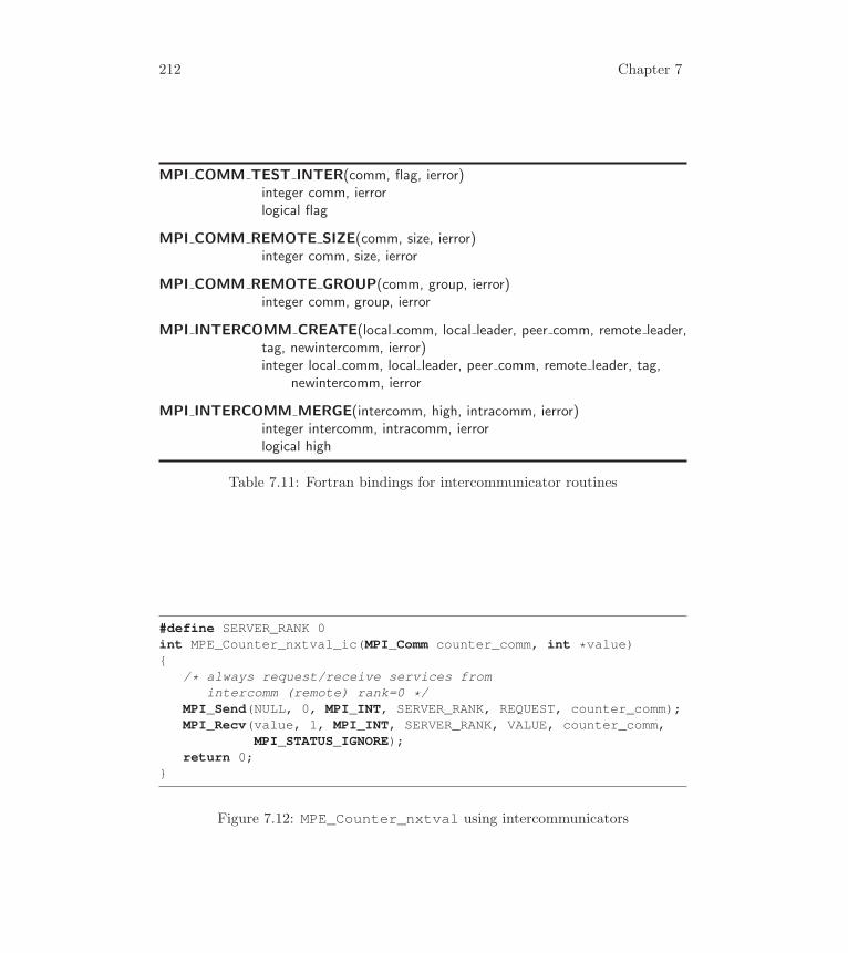
212 Chapter 7
MPI COMM TEST INTER(comm, flag, ierror)integer comm, ierrorlogical flag
MPI COMM REMOTE SIZE(comm, size, ierror)integer comm, size, ierror
MPI COMM REMOTE GROUP(comm, group, ierror)integer comm, group, ierror
MPI INTERCOMM CREATE(local comm, local leader, peer comm, remote leader,tag, newintercomm, ierror)integer local comm, local leader, peer comm, remote leader, tag,
newintercomm, ierror
MPI INTERCOMM MERGE(intercomm, high, intracomm, ierror)integer intercomm, intracomm, ierrorlogical high
Table 7.11: Fortran bindings for intercommunicator routines
#define SERVER_RANK 0int MPE_Counter_nxtval_ic(MPI_Comm counter_comm, int *value){
/* always request/receive services fromintercomm (remote) rank=0 */
MPI_Send(NULL, 0, MPI_INT, SERVER_RANK, REQUEST, counter_comm);MPI_Recv(value, 1, MPI_INT, SERVER_RANK, VALUE, counter_comm,
MPI_STATUS_IGNORE);return 0;
}
Figure 7.12: MPE_Counter_nxtval using intercommunicators
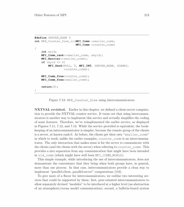
Other Features of MPI 213
#define SERVER_RANK 0int MPE_Counter_free_ic(MPI_Comm *smaller_comm,
MPI_Comm *counter_comm){
int myid;MPI_Comm_rank(*smaller_comm, &myid);MPI_Barrier(*smaller_comm);if (myid == 0)
MPI_Send(NULL, 0, MPI_INT, SERVER_RANK, GOAWAY,
*counter_comm);
MPI_Comm_free(counter_comm);MPI_Comm_free(smaller_comm);
return(0);}
Figure 7.13: MPE_Counter_free using intercommunicators
NXTVAL revisited. Earlier in this chapter, we defined a client-server computa-
tion to provide the NXTVAL counter service. It turns out that using intercommu-
nicators is another way to implement this service and actually simplifies the coding
of some features. Therefore, we’ve reimplemented the earlier service, as displayed
in Figures 7.11, 7.12, and 7.13. While the service provided is equivalent, the book-
keeping of an intercommunicator is simpler, because the remote group of the clients
is a server, at known rank 0. As before, the clients get their own “smaller_comm”in which to work; unlike the earlier examples, counter_comm is an intercommun-
icator. The only interaction that makes sense is for the server to communicate with
the clients (and the clients with the server) when referring to counter_comm. Thisprovides a nice separation from any communication that might have been intended
in old_comm (which might have well been MPI_COMM_WORLD).This simple example, while introducing the use of intercommunicators, does not
demonstrate the convenience that they bring when both groups have, in general,
more than one process. In that case, intercommunicators provide a clean way to
implement “parallel-client, parallel-server” computations [110].
To give more of a flavor for intercommunicators, we outline two interesting ser-
vices that could be supported by them: first, peer-oriented intercommunicators to
allow separately devised “modules” to be interfaced at a higher level (an abstraction
of an atmospheric/ocean model communication); second, a bulletin-board system

214 Chapter 7
analogous to the Linda tuple space [37].
Atmospheric and ocean intercommunication. A Grand Challenge applica-
tion that is often discussed is modeling the ocean and atmosphere in a single,
comprehensive code. Several groups are developing such codes, or evolving them
from their sequential counterparts—often the atmospheric and oceanic codes are
developed separately, with the intent to couple them at a higher level later on and
to transfer boundary information at the ocean-atmosphere boundary via messages.
Intercommunicators are natural for this situation. The separate codes can both
work with intracommunicators, allowing them to be developed and tested sepa-
rately. The intercommunicator for the ocean will have as its local group the ocean’s
processes, just as they appear in the intracommunicator used for ocean-only mes-
sages. Similarly, the intercommunicator for the atmosphere will have as its local
group the atmosphere’s processes. The remote group for the ocean will be the atmo-
spheric processes that interface on the ocean, and vice versa. Other strategies are
possible too, depending on the details of the communication across the boundary.
For example, assume that the two parts of the application have been written
to use a specified communicator comm instead of MPI_COMM_WORLD. We’ll name
the two parts do_ocean(comm) and do_atmos(comm). There is also a routine,
ocean_and_atmos(intercomm), that communicates data between the ocean
and atmosphere models. The main program that sets these up is shown in Fig-
ure 7.14.
Note that the result of MPI_Comm_split is a communicator that is either for
the ocean routine (if color = OCEAN) or for the atmosphere routine (if color= ATMOS). MPI_Comm_split always returns either a single new communicator
(if color is non-negative) or MPI_COMM_NULL.In Using Advanced MPI [55], we will see how to use the MPI dynamic pro-
cess features to bring together two separate MPI programs, rather than using this
approach of splitting MPI_COMM_WORLD.
Building a bulletin board (or Linda tuple space). A group of parallel data
servers is another possibility with intercommunicators. The Linda tuple space
model provides a bulletin board of data that can be accessed by name, in the
style of a virtual shared memory. In order to get reasonable scalability with this
strategy, multiple processes must be involved in the process of serving these re-
quests. Obvious operations are to place a named object into the space, to retrieve
its value, or to retrieve its value and remove it. A process that is a client of the
bulletin board service would have as its local group itself, or itself and others who
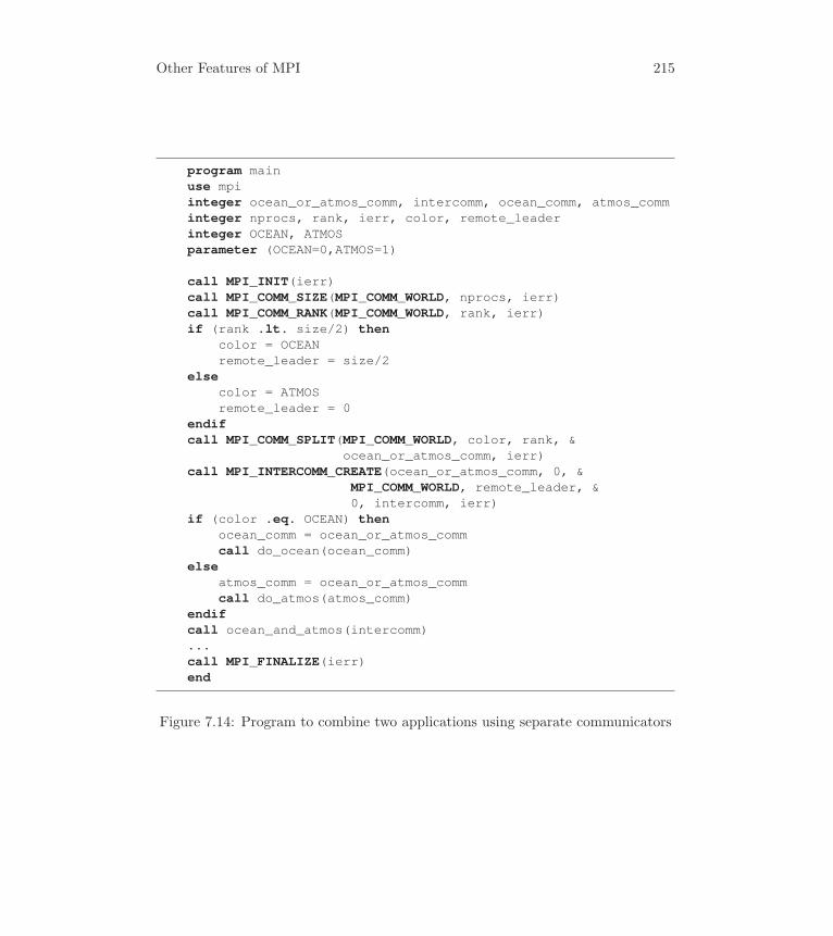
Other Features of MPI 215
program mainuse mpiinteger ocean_or_atmos_comm, intercomm, ocean_comm, atmos_comminteger nprocs, rank, ierr, color, remote_leaderinteger OCEAN, ATMOSparameter (OCEAN=0,ATMOS=1)
call MPI_INIT(ierr)call MPI_COMM_SIZE(MPI_COMM_WORLD, nprocs, ierr)call MPI_COMM_RANK(MPI_COMM_WORLD, rank, ierr)if (rank .lt. size/2) then
color = OCEANremote_leader = size/2
elsecolor = ATMOSremote_leader = 0
endifcall MPI_COMM_SPLIT(MPI_COMM_WORLD, color, rank, &
ocean_or_atmos_comm, ierr)call MPI_INTERCOMM_CREATE(ocean_or_atmos_comm, 0, &
MPI_COMM_WORLD, remote_leader, &0, intercomm, ierr)
if (color .eq. OCEAN) thenocean_comm = ocean_or_atmos_commcall do_ocean(ocean_comm)
elseatmos_comm = ocean_or_atmos_commcall do_atmos(atmos_comm)
endifcall ocean_and_atmos(intercomm)...call MPI_FINALIZE(ierr)end
Figure 7.14: Program to combine two applications using separate communicators
216 Chapter 7
are receiving the same class, or priority of service. The remote group for such
clients is the set of servers (or subset of servers) that is allowed to post and retrieve
information.
A key facet of these requests is that the clients need not know where the data
is and need not specify where it should be stored. Rather, a request will be made,
possibly to a master server, which will then scatter the request. One of the servers
will provide the service. The communication isolation of an intercommunicator
helps with the possibility that the client receive a response from any of the servers,
not just the server that took the client’s original request.
7.4 Heterogeneous Computing
Heterogeneous computing refers to using a collection of computers of different types
as a parallel computer. In many settings, a powerful parallel computer can be con-
structed by connecting workstations together. If workstations from several vendors
are combined, however, the workstations may not share a common format for data.
For example, the order of bytes within an integer may differ. Systems may even
use different numbers of bytes to represent integers and floating-point values.
MPI has been designed to operate correctly in this environment. MPI ensures
that if data is sent and received with MPI datatypes with the same type signature,
then the correct data will be received (if the data is representable on both the sender
and the receiver). No special steps need be taken to port an MPI program to a
heterogeneous parallel computer. Note also that this flexibility can be provided by
an MPI implementation at no cost on a homogeneous system; this helps encourage
the creation of programs that are truly portable between dedicated MPPs and
workstation clusters.
From the beginning, certain implementations of MPI supported heterogeneous
computing, including MPICH [59] and LAM [34]. Versions were also developed
that included support for more advanced security, resource, and scheduling issues;
see [50] for some of the issues and [48] for a description of one such implementation.
However, few current MPI implementations support systems that do not have
a common data format—the cost of creating, testing, and maintaining such an
implementation has been judged too high for the small demand for this feature.
This is a reflection of the convergence of the industry on a few standard formats
and the fact that most users of MPI have systems that are homogeneous in data
representation.

Other Features of MPI 217
7.5 Hybrid Programming with MPI and OpenMP
As we mentioned in Section 1.3.1, OpenMP is a compiler-based system for shared-
memory parallel programming with threads. As such it can be a convenient ap-
proach for exploiting the shared memory and multiple processing cores on the indi-
vidual nodes of a machine whose overall memory is distributed among such nodes.
In this case, MPI is used for the inter-node parallelism. The MPI and OpenMP
implementations must cooperate with one another in order to make this work, how-
ever. A full discussion of issues related to hybrid programming is given in Chapter 6
of Using Advanced MPI [55]. Here we present an abbreviated form of that mate-
rial. We will assume for the purposes of this section that you are at least modestly
familiar with OpenMP.
The MPI standard defines four levels of thread safety, any one of which per-
mits an MPI implementation to be compliant with the standard. Although the
standard definitions are independent of any particular thread model, they have a
straightforward interpretation for OpenMP. The four levels of thread safety are as
follows.
MPI_THREAD_SINGLE means that the MPI implementation expects only one user
thread to be present. This precludes the use of OpenMP.
MPI_THREAD_FUNNELED means that only the main OpenMP thread (called the
“master” in OpenMP) can make MPI calls. A thread can determine whether
it is the main thread or not by calling MPI_Is_thread_main. Most, if not
all, MPI implementations support this level of thread safety. That is, all MPI
calls are
• outside OpenMP parallel regions,
• inside OpenMP master regions, or
• guarded by a call to MPI_Is_thread_main. From MPI’s point of
view, the “main” thread is the one that called MPI_Init_thread (see
below).
MPI_THREAD_SERIALIZED means that only one thread may make MPI calls at
a time. For example,
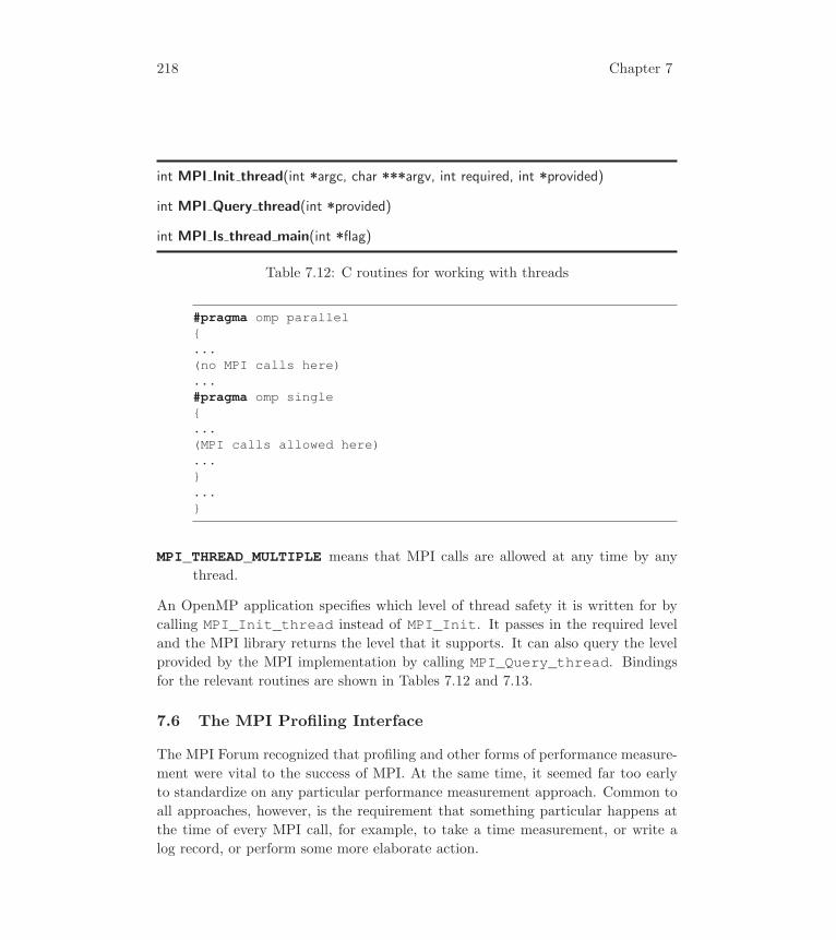
218 Chapter 7
int MPI Init thread(int *argc, char ***argv, int required, int *provided)
int MPI Query thread(int *provided)
int MPI Is thread main(int *flag)
Table 7.12: C routines for working with threads
#pragma omp parallel{...(no MPI calls here)...#pragma omp single{...(MPI calls allowed here)...}...}
MPI_THREAD_MULTIPLE means that MPI calls are allowed at any time by any
thread.
An OpenMP application specifies which level of thread safety it is written for by
calling MPI_Init_thread instead of MPI_Init. It passes in the required level
and the MPI library returns the level that it supports. It can also query the level
provided by the MPI implementation by calling MPI_Query_thread. Bindings
for the relevant routines are shown in Tables 7.12 and 7.13.
7.6 The MPI Profiling Interface
The MPI Forum recognized that profiling and other forms of performance measure-
ment were vital to the success of MPI. At the same time, it seemed far too early
to standardize on any particular performance measurement approach. Common to
all approaches, however, is the requirement that something particular happens at
the time of every MPI call, for example, to take a time measurement, or write a
log record, or perform some more elaborate action.
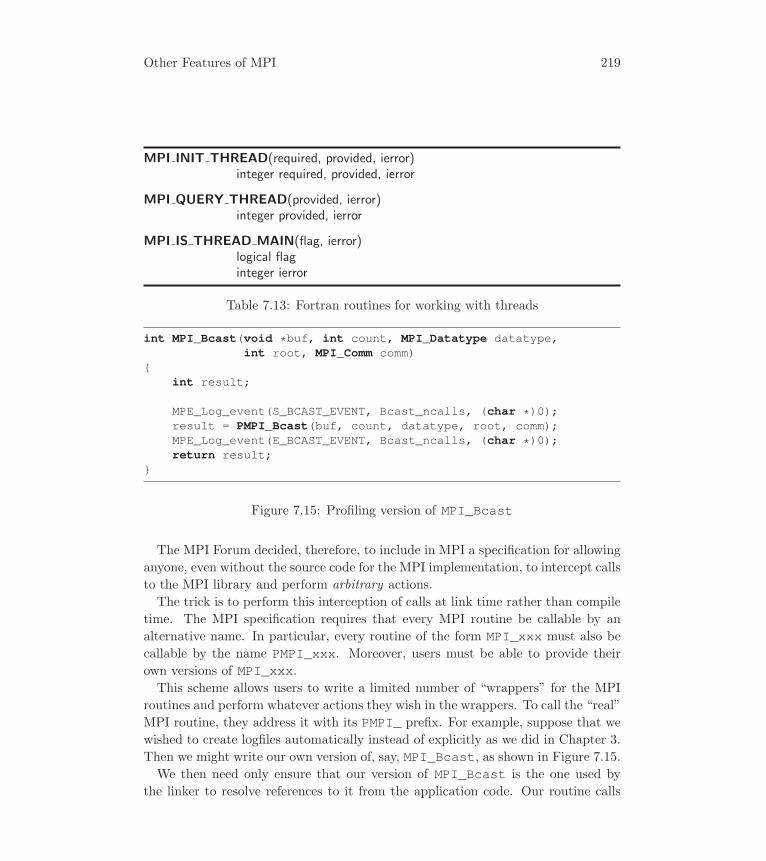
Other Features of MPI 219
MPI INIT THREAD(required, provided, ierror)integer required, provided, ierror
MPI QUERY THREAD(provided, ierror)integer provided, ierror
MPI IS THREAD MAIN(flag, ierror)logical flaginteger ierror
Table 7.13: Fortran routines for working with threads
int MPI_Bcast(void *buf, int count, MPI_Datatype datatype,int root, MPI_Comm comm)
{int result;
MPE_Log_event(S_BCAST_EVENT, Bcast_ncalls, (char *)0);result = PMPI_Bcast(buf, count, datatype, root, comm);MPE_Log_event(E_BCAST_EVENT, Bcast_ncalls, (char *)0);return result;
}
Figure 7.15: Profiling version of MPI_Bcast
The MPI Forum decided, therefore, to include in MPI a specification for allowing
anyone, even without the source code for the MPI implementation, to intercept calls
to the MPI library and perform arbitrary actions.
The trick is to perform this interception of calls at link time rather than compile
time. The MPI specification requires that every MPI routine be callable by an
alternative name. In particular, every routine of the form MPI_xxx must also be
callable by the name PMPI_xxx. Moreover, users must be able to provide their
own versions of MPI_xxx.This scheme allows users to write a limited number of “wrappers” for the MPI
routines and perform whatever actions they wish in the wrappers. To call the “real”
MPI routine, they address it with its PMPI_ prefix. For example, suppose that we
wished to create logfiles automatically instead of explicitly as we did in Chapter 3.
Then we might write our own version of, say, MPI_Bcast, as shown in Figure 7.15.
We then need only ensure that our version of MPI_Bcast is the one used by
the linker to resolve references to it from the application code. Our routine calls
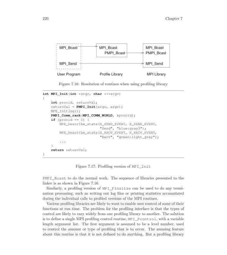
220 Chapter 7
User Program MPI LibraryProfile Library
MPI_Bcast
MPI_Send
MPI_BcastPMPI_Bcast
MPI_BcastPMPI_Bcast
MPI_Send
Figure 7.16: Resolution of routines when using profiling library
int MPI_Init(int *argc, char ***argv){
int procid, returnVal;returnVal = PMPI_Init(argc, argv);MPE_Initlog();PMPI_Comm_rank(MPI_COMM_WORLD, &procid);if (procid == 0) {
MPE_Describe_state(S_SEND_EVENT, E_SEND_EVENT,"Send", "blue:gray3");
MPE_Describe_state(S_RECV_EVENT, E_RECV_EVENT,"Recv", "green:light_gray");
...}return returnVal;
}
Figure 7.17: Profiling version of MPI_Init
PMPI_Bcast to do the normal work. The sequence of libraries presented to the
linker is as shown in Figure 7.16.
Similarly, a profiling version of MPI_Finalize can be used to do any termi-
nation processing, such as writing out log files or printing statistics accumulated
during the individual calls to profiled versions of the MPI routines.
Various profiling libraries are likely to want to enable user control of some of their
functions at run time. The problem for the profiling interface is that the types of
control are likely to vary widely from one profiling library to another. The solution
is to define a single MPI profiling control routine, MPI_Pcontrol, with a variable
length argument list. The first argument is assumed to be a level number, used
to control the amount or type of profiling that is to occur. The amusing feature
about this routine is that it is not defined to do anything. But a profiling library

Other Features of MPI 221
int MPI Pcontrol(const int level, . . . )
Table 7.14: C binding for MPI profiling control
MPI PCONTROL(level)integer level
Table 7.15: Fortran binding for MPI profiling control. Note that this is one of thefew MPI routines whose Fortran binding does not include an error return code.
writer can redefine it, just as he redefines other MPI routines. The bindings for
MPI_Pcontrol are shown in Tables 7.14 and 7.15.
The beauty of this arrangement is that the supplier of the profiling library need not
provide profiling versions of any routines other than those in which he is interested.
Once the style of profiling has been chosen, of course, most of what goes into
the profiled version of each routine is the same. It is not difficult to develop a
metaprofiling mechanism that automates the wrapping of all, or a specific subset,
of the MPI routines at once, provided that the action taken for each routine is the
same.
The profiling interface can also be used to answer questions about an application
without changing the source code of the application. We will illustrate this with
two examples.
7.6.1 Finding Buffering Problems
The routine MPI_Send is often implemented with some internal buffering, allowing
some programs that are formally unsafe (because they depend on buffering) to run
in practice. Depending on such buffering is poor practice, however. Is there any
easy way to check to see whether a program depends on buffering in MPI_Send?This is a hard problem to answer in general, but the following approaches will
often reveal codes that depend on buffering. Our first solution is very simple. We
will write our own version of MPI_Send that provides no buffering:
subroutine MPI_SEND(buf, count, datatype, dest, &tag, comm, ierr)
use mpi, only : PMPI_SSENDinteger buf(*), count, datatype, dest, tag, comm, ierrcall PMPI_SSEND(buf, count, datatype, dest, tag, comm, ierr)end

222 Chapter 7
int MPI Issend(const void* buf, int count, MPI Datatype datatype, int dest, int tag,
MPI Comm comm, MPI Request *request)
Table 7.16: C binding for the nonblocking synchronous send
With this version of MPI_Send, many programs that depend on MPI_Send pro-
viding buffering will deadlock; specifically, the program will enter this routine but
never complete because the matching receive, required to start before MPI_Ssendand PMPI_Ssend can complete, is never started. If a parallel debugger is available,
it can be used to find out where the program has stopped.
We’ve shown the use of the mpi module assuming that the module fully imple-
ments the Fortran MPI bindings as described in the standard. Unfortunately, it is
difficult to implement the mpi module using standard Fortran. As a result, many
MPI implementations implement as much of the mpimodule as possible, often leav-
ing out the interface definitions for routines that have “choice” parameters—such
as communication buffers that can be of any type. In that case, the examples here
may fail to compile, because the routine definition is not in the module. You then
have several options. One is to fall back on the mpif.h include file. The other is
to adapt your code to extract only the values, not the routine definitions from the
mpi module. For example, in Figure 7.18, the use statement could be
use mpi, only: MPI_STATUS_SIZE, PMPI_WTIME
The value MPI_STATUS_SIZE is needed for the status declaration, and PMPI_-WTIME is needed to declare this routine as a function that returns a doubleprecision value.
The approach of using MPI_Ssend is a little awkward because it depends on
having the program deadlock and then using a parallel debugger. Can we write a
version of MPI_Send that will detect that a problem exists? We can, if we require
that any MPI_Send complete within a specific length of time. For example, in many
scientific applications, no send operation should take more than a few seconds. Let
us assume that any MPI_Ssend that takes more than ten seconds indicates a
problem. Hence, what we need is a send operation that is nonblocking (so that we
can start it and then time how long it takes, waiting no more than ten seconds)
and that cannot complete until the matching receive begins. In other words, we
want to use the nonblocking synchronous send MPI_Issend. The bindings for thisroutine are the same as for the other nonblocking sends, as shown in Tables 7.16
and 7.17.
Other Features of MPI 223
MPI ISSEND(buf, count, datatype, dest, tag, comm, request, ierror)
<type> buf(*)integer count, datatype, dest, tag, comm, request, ierror
Table 7.17: Fortran binding for the nonblocking synchronous send
The code is shown in Figure 7.18. This code busy-waits for the PMPI_Issendto complete by calling PMPI_Test repeatedly. More refined versions might poll
PMPI_Test for a short period of time, then sleep (using the Unix sleep call)
for a second or two, then test again, and so on, until ten seconds elapse. Another
version could use MPI_Pcontrol to allow the user to control the length of time
delay rather than fixing the time limit at ten seconds.
7.6.2 Finding Load Imbalances
Consider an application that uses MPI_Allreduce and where profiling results,
using, for example, the MPE profiling library, indicate that MPI_Allreduce is
very slow, hurting parallel performance. In many cases, the problem is not in the
implementation of MPI_Allreduce; rather, the problem is in a load imbalance in
the application. Because MPI_Allreduce is synchronizing (since no process can
complete this operation before all processes have contributed their values), any load
imbalance shows up in the execution time of MPI_Allreduce. We can estimate
the size of the load imbalance by measuring the time that an MPI_Barrier takes
right before the MPI_Allreduce. Figure 7.19 shows one simple implementation;
it also shows how to use MPI_Finalize to report final statistics.
7.6.3 Mechanics of Using the Profiling Interface
The MPI standard does not specify how to compile or link programs with MPI
(other than specifying that the header files mpi.h and mpif.h and the Fortran
modules mpi and mpi_f08 must exist, if the MPI implementation supports those
levels of Fortran). Similarly, the names of the MPI library and the name of any
separate library containing the profiling versions of the MPI routines are not spec-
ified.
Some implementations provide compiler wrappers that ensure that all of the
libraries and any other options are properly applied. For example, to compile a C
program in file myprog.c, you might use
mpicc -o myprog myprog.c
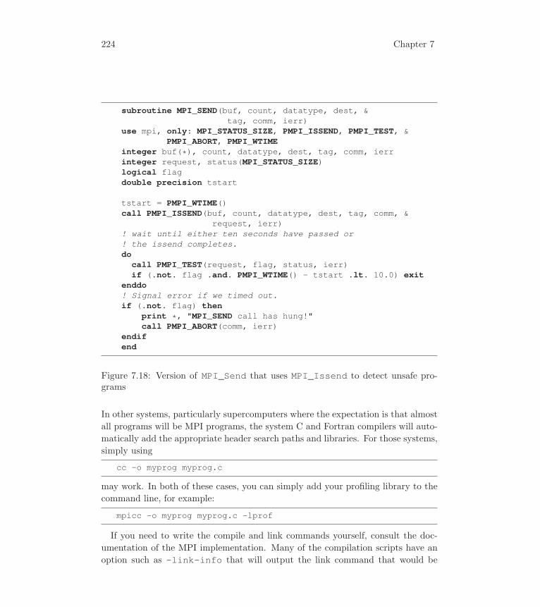
224 Chapter 7
subroutine MPI_SEND(buf, count, datatype, dest, &tag, comm, ierr)
use mpi, only: MPI_STATUS_SIZE, PMPI_ISSEND, PMPI_TEST, &PMPI_ABORT, PMPI_WTIME
integer buf(*), count, datatype, dest, tag, comm, ierrinteger request, status(MPI_STATUS_SIZE)logical flagdouble precision tstart
tstart = PMPI_WTIME()call PMPI_ISSEND(buf, count, datatype, dest, tag, comm, &
request, ierr)! wait until either ten seconds have passed or! the issend completes.do
call PMPI_TEST(request, flag, status, ierr)if (.not. flag .and. PMPI_WTIME() - tstart .lt. 10.0) exit
enddo! Signal error if we timed out.if (.not. flag) then
print *, "MPI_SEND call has hung!"call PMPI_ABORT(comm, ierr)
endifend
Figure 7.18: Version of MPI_Send that uses MPI_Issend to detect unsafe pro-grams
In other systems, particularly supercomputers where the expectation is that almost
all programs will be MPI programs, the system C and Fortran compilers will auto-
matically add the appropriate header search paths and libraries. For those systems,
simply using
cc -o myprog myprog.c
may work. In both of these cases, you can simply add your profiling library to the
command line, for example:
mpicc -o myprog myprog.c -lprof
If you need to write the compile and link commands yourself, consult the doc-
umentation of the MPI implementation. Many of the compilation scripts have an
option such as -link-info that will output the link command that would be

Other Features of MPI 225
static double t_barrier = 0, t_allreduce = 0;int MPI_Allreduce(const void* sendbuf, void* recvbuf, int count,
MPI_Datatype datatype, MPI_Op op, MPI_Comm comm){
double t1, t2, t3;t1 = PMPI_Wtime();PMPI_Barrier(comm);t2 = PMPI_Wtime();PMPI_Allreduce(sendbuf, recvbuf, count, datatype, op, comm);t3 = PMPI_Wtime();t_barrier += (t2 - t1);t_allreduce += (t3 - t2);if (t3 - t2 < t2 - t1) {
int myrank;PMPI_Comm_rank(comm, &myrank);printf("Barrier slower than Allreduce on %d\n", myrank);
}return MPI_SUCCESS;
}int MPI_Finalize(){
int rank;PMPI_Comm_rank(MPI_COMM_WORLD, &rank);printf("[%d]: Allreduce barrier time %f; Allreduce time %f\n",
rank, t_barrier, t_allreduce);return PMPI_Finalize();
}
Figure 7.19: C version of MPI_Allreduce that uses PMPI_Barrier to estimatethe amount of load imbalance
used to link an MPI program. When examining the link command, note that there
are no standards for the library names or order (one implementation, MPICH, has
created an optional standard for all implementations that use MPICH as the basis
for their implementation). In some systems, both the MPI and PMPI routines will
be in a single library. This is the simplest case. In other cases, the PMPI routines
will be in a separate library. For example, let us assume that the MPI routines are
in libmpi and the PMPI versions are in libpmpi. Then a link line for a program
in myprog.o with a profiling library libprof might look like
cc -o myprog myprog.o -lprof -lmpi -lpmpi

226 Chapter 7
Note that the profiling library -lpmpi follows the regular (-lmpi) library. In
some cases, it may be necessary to repeat the library names. Using Fortran may
also require special libraries. You should check the documentation for your MPI
implementation; do not assume that cc ... -lmpi -lpmpi is all that you
need to do.
7.7 Error Handling
Error handling and error recovery are important and difficult issues. Errors can be
the result of user mistakes (e.g., invalid arguments), hardware errors (e.g., power
supply failure), resource exhaustion (e.g., no more memory), or bugs in the base
software. MPI provides some facilities for handling error reporting, particularly by
libraries.
7.7.1 Error Handlers
MPI associates an error handler with each communicator. When an error is de-
tected, MPI calls the error handler associated with the communicator being used; if
there is no communicator, MPI_COMM_WORLD is used. When MPI_Init is called,
the initial (default) error handler is one that causes the program to abort (i.e., all
processes exit). Most MPI implementations will print an error message as well.
Instead of aborting on an error, MPI can return an error code. In Fortran, this
is the ierror argument in most of the MPI routines. In C, this is the return
value of the MPI function. The only exceptions are MPI_Wtime, MPI_Wtick, andthe handle transfer routines (these are routines used to convert MPI handles, such
as an MPI_Request, between Fortran and C). MPI provides two predefined error
handlers: MPI_ERRORS_ARE_FATAL (the default) and MPI_ERRORS_RETURN.MPI_ERRORS_RETURN causes the MPI routines to return an error value instead of
aborting. The routine MPI_Comm_set_errhandler is used to change the error
handler.
The error codes returned, with the exception of MPI_SUCCESS, are defined by
each MPI implementation. This approach allows an MPI implementation to encode
additional data into the error code. MPI also specifies a small set of error classes:
integers that divide the errors codes into a small number of categories. For example,
for an error class such as MPI_ERR_TAG, the error code could encode information
on what was wrong with the tag value (e.g., too big? too small?) and the MPI
routine that detected the error. The error classes used by the routines in this book

Other Features of MPI 227
MPI_SUCCESS No errorMPI_ERR_BUFFER Invalid buffer pointerMPI_ERR_COUNT Invalid count argumentMPI_ERR_TYPE Invalid datatype argumentMPI_ERR_TAG Invalid tag argumentMPI_ERR_COMM Invalid communicatorMPI_ERR_RANK Invalid rankMPI_ERR_REQUEST Invalid request (handle)MPI_ERR_ROOT Invalid rootMPI_ERR_GROUP Invalid groupMPI_ERR_OP Invalid operationMPI_ERR_TOPOLOGY Invalid topologyMPI_ERR_DIMS Invalid dimension argumentMPI_ERR_ARG Invalid argument of some other kindMPI_ERR_UNKNOWN Unknown errorMPI_ERR_TRUNCATE Message truncated on receiveMPI_ERR_OTHER Known error not in this listMPI_ERR_INTERN Internal MPI errorMPI_ERR_IN_STATUS Look in the status array for the errorMPI_ERR_PENDING Operation not complete (see text)MPI_ERR_KEYVAL Invalid keyval usedMPI_ERR_LASTCODE Last standard error code (not class)
Table 7.18: Error classes for the routines in this book
are shown in Table 7.18. MPI-2 and MPI-3 added additional error classes; these
are covered in Using Advanced MPI [55].
The difference between the classes MPI_ERR_UNKNOWN and MPI_ERR_OTHER is
that MPI_Error_string can return useful information about MPI_ERR_OTHER.The error class MPI_ERR_UNKNOWN can be used by an MPI implementation for un-
expected situations, such as an error return from code that the MPI implementation
itself uses.
The two error classes MPI_ERR_IN_STATUS and MPI_ERR_PENDING are spe-
cial cases. MPI has four routines that complete multiple requests and return an
array of statuses; these are MPI_Waitsome, MPI_Waitall, MPI_Testsome, andMPI_Testall. For these four functions, errors could occur for any subset of the
requests. In this case, there is no single error code to return from the routine. In
this case, the error value returned is MPI_ERR_IN_STATUS. This indicates that
the actual error codes are in the array of statuses, in the MPI_ERROR element

228 Chapter 7
/* Install a new error handler */MPI_Comm_set_errhandler(MPI_COMM_WORLD, MPI_ERRORS_RETURN);/* Send a message to an invalid destination */dest = -1;errcode = MPI_Send(..., dest, ...);if (errcode != MPI_SUCCESS) {
MPI_Error_class(errcode, &errclass);if (errclass == MPI_ERR_RANK) {
printf("Invalid rank (%d) in call to MPI_Send", dest);}
}
Figure 7.20: Code to check the error class of an error code returned by an MPIroutine. Note that the MPI standard does not specify which error class a particularerror returns; other possibilities for this error include MPI_ERR_ARG.
(status.MPI_ERROR in C; status(MPI_ERROR) in Fortran). To understand
MPI_ERR_PENDING, consider the case of MPI_Waitall. For each request that
was passed to MPI_Waitall, three possibilities exist. First, the request com-
pleted successfully. In this case, the MPI_ERROR field of the corresponding status
element is set to MPI_SUCCESS. Second, the request failed because of an error;
in this case, the MPI_ERROR field of the corresponding status element is set to
the MPI error code that indicates the reason the request failed. Third, the re-
quest has neither completed nor failed; in this case, the MPI_ERROR field is set to
MPI_ERR_PENDING to indicate that the request is still pending without error.
To convert an error code into an error class, use MPI_Error_class. As an
example, consider the code in Figure 7.20.
All MPI implementations provide a way to translate an MPI error code or class
into a string. The routine MPI_Error_string takes an error code or class and
a user-provided string buffer and returns a description of the error in the string,
along with the length of the text in the string. The string buffer must be MPI_-MAX_ERROR_STRING in size.
For example, instead of using MPI_Error_class in the example above, we
could use
...if (errcode != MPI_SUCCESS) {
MPI_Error_class(errcode, &errclass);if (errclass == MPI_ERR_RANK) {
char buffer[MPI_MAX_ERROR_STRING];

Other Features of MPI 229
int resultlen;MPI_Error_string(errcode, buffer, &resultlen);puts(buffer);
}}
The value of MPI_MAX_ERROR_STRING in C is one greater than the value of
MPI_MAX_ERROR_STRING in Fortran to allow for the string terminator in C.
That is, the same maximum number of characters are allowed in both C and For-
tran; however, C requires a declaration of char buf[11] to hold ten characters
while Fortran requires character*10 buf. Fortran users should also note that
character*10 buf and character buf(10) are very different declarations.
Error strings in Fortran must be declared as
character*(MPI_MAX_ERROR_STRING) buf
7.7.2 Example of Error Handling
Figure 7.21 shows code that reports on any errors that occur during the execution
of one of the four MPI routines that can complete multiple requests. This code
assumes that the error handler has been set to be MPI_ERRORS_RETURN.
7.7.3 User-Defined Error Handlers
MPI also allows the user to define additional error handlers.
A user-defined error handler for communicators has the form
void user_function(MPI_Comm *comm, int *error_code, ...)
The first argument is the communicator of the operation; the second is the error
code. Pointers are used so that Fortran programmers may write MPI error han-
dlers without resorting to C. Additional arguments are available to C programmers
through a “stdargs” interface; their meaning is defined by each MPI implementa-
tion.
Often, it is desirable to temporarily replace one error handler with another one.
For example, in Fortran we can use
integer old_handler, new_handlercall MPI_Comm_get_errhandler(comm, old_handler, ierr)call MPI_Comm_set_errhandler(comm, new_handler, ierr)<.... code .... >call MPI_Comm_set_errhandler(comm, old_handler, ierr)

230 Chapter 7
MPI_Request req_array[100];MPI_Status status_array[100];char msg[MPI_MAX_ERROR_STRING];...err = MPI_Waitall(n, req_array, status_array);if (err == MPI_ERR_IN_STATUS) {
for (i=0; i<n; i++) {switch (status_array[i].MPI_ERROR) {case MPI_SUCCESS: /* request has completed */break;case MPI_ERR_PENDING: /* request hasn’t completed */break;default: /* error on this request */MPI_Error_string(status_array[i].MPI_ERROR, msg,
&msglen);printf("Error in request %d: %s\n", i, msg);}
}}
Figure 7.21: Handling error returns from MPI_Waitany
call MPI_Errhandler_free(old_handler, ierr)
An MPI error handler is an opaque object that is created and freed much like an
MPI_Request. The routine MPI_Comm_create_errhandler creates an MPI
error handler that Fortran and C users can assign to a variable.
Once an error handler is created, it can be attached to a communicator with
MPI_Comm_set_errhandler. This is done so that a library that uses its own
communicator can have its own error handler. The error handler for a communi-
cator can be retrieved with MPI_Comm_get_errhandler and freed with MPI_-Errhandler_free.The last line of this example calls MPI_Errhandler_free to free the error
handler returned by MPI_Comm_set_errhandler. In general, most MPI rou-
tines that return an MPI object, such as the group associated with a communica-
tor (MPI_Comm_group and MPI_Comm_remote_group), return (semantically3)
a copy of the object; this copy must be freed by the user when it is no longer
3By this we mean that the object behaves as if it is a copy. An implementation can implementthis operation in many ways; many implementations use a reference count mechanism to avoidmaking an actual copy.

Other Features of MPI 231
needed. The MPI-3 standard clarified the previous versions of the standard to say
that an error handler returned by MPI_Comm_get_errhandler should be freed
with MPI_Errhandler_free when it is no longer needed.
Error handlers are inherited from the parent communicator. That is, when a new
communicator is created with a function such as MPI_Comm_dup, the error handlerin the new communicator is set to be the same one as the input communicator.
Thus, to change the “global” error handler, one might change the error handler
associated with MPI_COMM_WORLD before any other communicators are created
(for example, right after the MPI_Init call). Error handlers may also be defined
for two other classes of routines in MPI; see Using Advanced MPI [55] for details.
Users should be careful with error handlers. The MPI standard does not require
that a program that encounters an error be continuable; that is, once an error has
occurred, it may not be possible for the program to continue to use MPI. This
is a common position for standards: a standard does not specify the behavior of
erroneous programs.
In the most general case, where nothing is known about the ability of the MPI
implementation to continue from errors, the user should terminate the program
(see the next section). User-defined error handlers can be used to ensure that
program termination proceeds in an orderly way and that important information
is preserved. For example, a user-defined error handler might flush all file output
buffers and write out some information on the cause of the error.
However, most MPI implementations will allow a program to continue and oper-
ate correctly after an error is encountered. In fact, many of the error classes repre-
sent cases where error recovery is particularly easy. These classes include all of the
“invalid xxx” errors: MPI_ERR_BUFFER, MPI_ERR_COUNT, MPI_ERR_TYPE, . . .,MPI_ERR_ARG. Most MPI implementations will also continue after MPI_ERR_-TRUNCATE, which is usually generated when the specified buffer size in a receive
operation is too small to hold the message received (the usual behavior is to dis-
card either the entire message or the part that does not fit in the buffer). The error
classes MPI_ERR_UNKNOWN and MPI_ERR_INTERN are usually not continuable
since they indicate a problem within the MPI implementation itself. The other
error class, MPI_ERR_OTHER, may or may not be continuable, depending on the
particular MPI implementation. The behavior of MPI in the presence of faults is
discussed in Section 9.2.
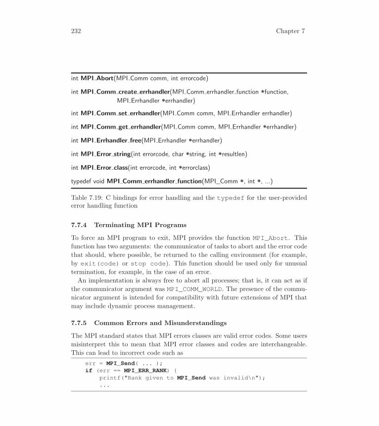
232 Chapter 7
int MPI Abort(MPI Comm comm, int errorcode)
int MPI Comm create errhandler(MPI Comm errhandler function *function,
MPI Errhandler *errhandler)
int MPI Comm set errhandler(MPI Comm comm, MPI Errhandler errhandler)
int MPI Comm get errhandler(MPI Comm comm, MPI Errhandler *errhandler)
int MPI Errhandler free(MPI Errhandler *errhandler)
int MPI Error string(int errorcode, char *string, int *resultlen)
int MPI Error class(int errorcode, int *errorclass)
typedef void MPI Comm errhandler function(MPI_Comm *, int *, ...)
Table 7.19: C bindings for error handling and the typedef for the user-providederror handling function
7.7.4 Terminating MPI Programs
To force an MPI program to exit, MPI provides the function MPI_Abort. This
function has two arguments: the communicator of tasks to abort and the error code
that should, where possible, be returned to the calling environment (for example,
by exit(code) or stop code). This function should be used only for unusual
termination, for example, in the case of an error.
An implementation is always free to abort all processes; that is, it can act as if
the communicator argument was MPI_COMM_WORLD. The presence of the commu-
nicator argument is intended for compatibility with future extensions of MPI that
may include dynamic process management.
7.7.5 Common Errors and Misunderstandings
The MPI standard states that MPI errors classes are valid error codes. Some users
misinterpret this to mean that MPI error classes and codes are interchangeable.
This can lead to incorrect code such as
err = MPI_Send( ... );if (err == MPI_ERR_RANK) {
printf("Rank given to MPI_Send was invalid\n");...
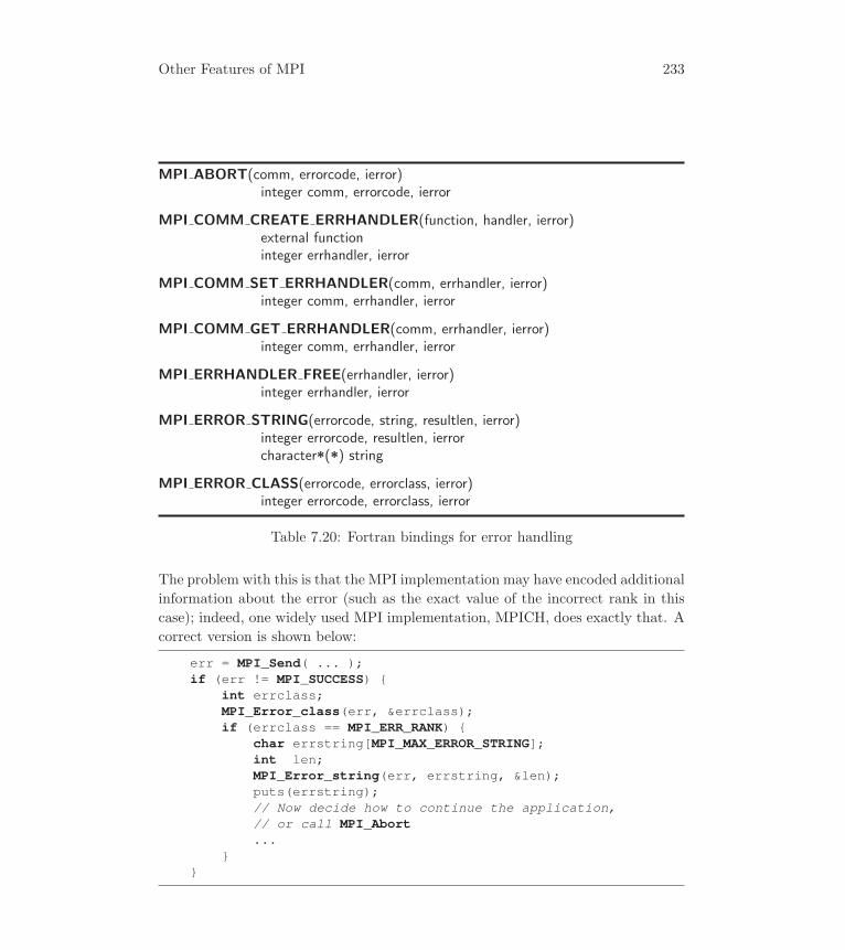
Other Features of MPI 233
MPI ABORT(comm, errorcode, ierror)integer comm, errorcode, ierror
MPI COMM CREATE ERRHANDLER(function, handler, ierror)external functioninteger errhandler, ierror
MPI COMM SET ERRHANDLER(comm, errhandler, ierror)integer comm, errhandler, ierror
MPI COMM GET ERRHANDLER(comm, errhandler, ierror)integer comm, errhandler, ierror
MPI ERRHANDLER FREE(errhandler, ierror)integer errhandler, ierror
MPI ERROR STRING(errorcode, string, resultlen, ierror)integer errorcode, resultlen, ierrorcharacter*(*) string
MPI ERROR CLASS(errorcode, errorclass, ierror)integer errorcode, errorclass, ierror
Table 7.20: Fortran bindings for error handling
The problem with this is that the MPI implementation may have encoded additional
information about the error (such as the exact value of the incorrect rank in this
case); indeed, one widely used MPI implementation, MPICH, does exactly that. A
correct version is shown below:
err = MPI_Send( ... );if (err != MPI_SUCCESS) {
int errclass;MPI_Error_class(err, &errclass);if (errclass == MPI_ERR_RANK) {
char errstring[MPI_MAX_ERROR_STRING];int len;MPI_Error_string(err, errstring, &len);puts(errstring);// Now decide how to continue the application,// or call MPI_Abort...
}}

234 Chapter 7
This version also makes use of MPI_Error_string to print a more detailed error
message in the event that the MPI implementation provides it. The only error
classes that may be compared to the error codes output by an MPI routine are
MPI_SUCCESS and MPI_ERR_IN_STATUS.
7.8 The MPI Environment
In writing portable programs, one often needs to determine some implementation
limits. For example, even a sequential program may need to know how many
open files it can have. In many cases, this information is available only from the
documentation of the system; and this documentation may be incorrect or out of
date. MPI provides access to some of the implementation limits through predefined
attribute keys defined for the communicator MPI_COMM_WORLD (see Section 6.2 for
information about attribute keys).
Currently, MPI has only six predefined attribute keys:
MPI_TAG_UB Largest message tag value (smallest is zero).
MPI_HOST Rank in MPI_COMM_WORLD of host process, if any.
MPI_IO Which process can do I/O (see below).
MPI_WTIME_IS_GLOBAL If true, the values returned by MPI_Wtime are synchro-
nized across all processes in MPI_COMM_WORLD (that is, MPI_Wtime returns
the value of a global clock).
MPI_APPNUM If the MPI job contains multiple executables, this gives the index,
starting from zero, of the executable being run by this process. MPI programs
can be started with multiple executables either with mpiexec or with MPI_-Comm_spawn_multiple, described in Using Advanced MPI [55]. For most
applications in this book, the value of this attribute will either be zero or the
attribute will not be set.
MPI_UNIVERSE_SIZE Used to indicated how many processes might be created
with MPI’s dynamic process routines. See Using Advanced MPI [55] for more
details.
Some parallel processing systems have a distinguished process called the host. The
value of MPI_HOST is the rank of this process in MPI_COMM_WORLD. If there is no
host process, the value MPI_PROC_NULL is used.

Other Features of MPI 235
MPI makes some requirements for how system operations are provided if they
are provided. For example, any system operation, whether it be (in C) a mallocor a printf or (in Fortran) an open or write, must operate independently of
other processes. This means that all I/O is independent if it can be performed at
all. To determine whether I/O is available, one uses the attribute key MPI_IO.The value associated with this key can be MPI_ANY_SOURCE, indicating that any
and all processes can perform I/O; MPI_PROC_NULL, indicating that no process
can perform I/O; or a rank of a process that can perform I/O.
The definition of “perform I/O” is that any of the language-specified I/O oper-
ations are allowed. For example, for C users, this means that printf and scanfare supported. For Fortran, this means that read (including read *, ...) and
print are supported. If a system cannot provide the full functionality of the
language-specified I/O, it is required to return MPI_PROC_NULL as the value of
the key MPI_IO. (This does not mean that the system cannot provide any I/O,
just that it must return MPI_PROC_NULL if it cannot provide all of the language-
specified I/O. On some systems, providing access to standard input is not possible;
these systems must return MPI_PROC_NULL.)When MPI was first specified, some parallel computers did not have good fa-
cilities for providing I/O to all MPI processes or could provide only a subset of
the language-specified I/O. Some MPI implementations also chose not to provide
I/O from every process. While in some cases I/O is still not available from each
process, these are now much less common. Many MPI applications assume that
I/O is available from every process and operate on a wide variety of platforms.
Note that because the key values are defined by MPI, future versions of MPI can
define additional key values. In fact, MPI_WTIME_IS_GLOBAL is an example; this
key value was added in MPI 1.1. In addition, each MPI implementation may define
key values that refer to a particular implementation. As a hypothetical example,
an implementation might provide MPIV_REQUESTS (MPIV for MPI vendor) that
would give the number of MPI_Requests that can be active at any time. To
date, few such vendor-specific key values have been implemented, although some
research projects did investigate the use of key values to provide run-time control
of parameters within a particular MPI implementation to an application. Instead,
a different mechanism, MPI_Info, which was added in MPI-2 and expanded in
MPI-3, is used for some cases; and MPI-3 added a very general mechanism, called
the MPIT or “tools interface,” which provides direct ways to query and set param-
eters that control the execution of the MPI implementation. These approaches are
described in Using Advanced MPI [55].
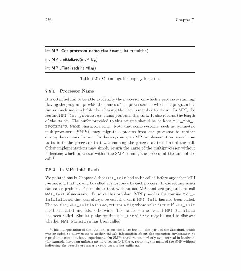
236 Chapter 7
int MPI Get processor name(char *name, int *resultlen)
int MPI Initialized(int *flag)
int MPI Finalized(int *flag)
Table 7.21: C bindings for inquiry functions
7.8.1 Processor Name
It is often helpful to be able to identify the processor on which a process is running.
Having the program provide the names of the processors on which the program has
run is much more reliable than having the user remember to do so. In MPI, the
routine MPI_Get_processor_name performs this task. It also returns the length
of the string. The buffer provided to this routine should be at least MPI_MAX_-PROCESSOR_NAME characters long. Note that some systems, such as symmetric
multiprocessors (SMPs), may migrate a process from one processor to another
during the course of a run. On these systems, an MPI implementation may choose
to indicate the processor that was running the process at the time of the call.
Other implementations may simply return the name of the multiprocessor without
indicating which processor within the SMP running the process at the time of the
call.4
7.8.2 Is MPI Initialized?
We pointed out in Chapter 3 that MPI_Init had to be called before any other MPI
routine and that it could be called at most once by each process. These requirements
can cause problems for modules that wish to use MPI and are prepared to call
MPI_Init if necessary. To solve this problem, MPI provides the routine MPI_-Initialized that can always be called, even if MPI_Init has not been called.
The routine, MPI_Initialized, returns a flag whose value is true if MPI_Inithas been called and false otherwise. The value is true even if MPI_Finalizehas been called. Similarly, the routine MPI_Finalized may be used to discover
whether MPI_Finalize has been called.
4This interpretation of the standard meets the letter but not the spirit of the Standard, whichwas intended to allow users to gather enough information about the execution environment toreproduce a computational experiment. On SMPs that are not perfectly symmetrical in hardware(for example, have non-uniform memory access (NUMA)), returning the name of the SMP withoutindicating the specific processor or chip used is not sufficient.
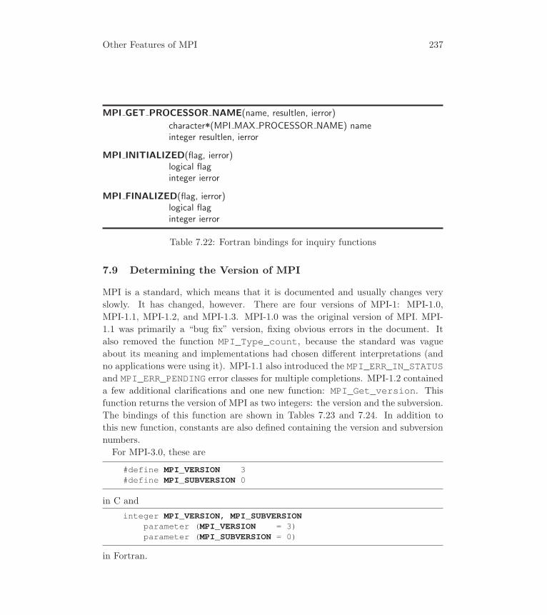
Other Features of MPI 237
MPI GET PROCESSOR NAME(name, resultlen, ierror)
character*(MPI MAX PROCESSOR NAME) nameinteger resultlen, ierror
MPI INITIALIZED(flag, ierror)logical flaginteger ierror
MPI FINALIZED(flag, ierror)logical flaginteger ierror
Table 7.22: Fortran bindings for inquiry functions
7.9 Determining the Version of MPI
MPI is a standard, which means that it is documented and usually changes very
slowly. It has changed, however. There are four versions of MPI-1: MPI-1.0,
MPI-1.1, MPI-1.2, and MPI-1.3. MPI-1.0 was the original version of MPI. MPI-
1.1 was primarily a “bug fix” version, fixing obvious errors in the document. It
also removed the function MPI_Type_count, because the standard was vague
about its meaning and implementations had chosen different interpretations (and
no applications were using it). MPI-1.1 also introduced the MPI_ERR_IN_STATUSand MPI_ERR_PENDING error classes for multiple completions. MPI-1.2 contained
a few additional clarifications and one new function: MPI_Get_version. This
function returns the version of MPI as two integers: the version and the subversion.
The bindings of this function are shown in Tables 7.23 and 7.24. In addition to
this new function, constants are also defined containing the version and subversion
numbers.
For MPI-3.0, these are
#define MPI_VERSION 3#define MPI_SUBVERSION 0
in C and
integer MPI_VERSION, MPI_SUBVERSIONparameter (MPI_VERSION = 3)parameter (MPI_SUBVERSION = 0)
in Fortran.
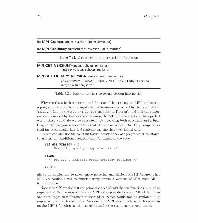
238 Chapter 7
int MPI Get version(int *version, int *subversion)
int MPI Get library version(char *version, int *resultlen)
Table 7.23: C routines to return version information
MPI GET VERSION(version, subversion, ierror)integer version, subversion, ierror
MPI GET LIBRARY VERSION(version, resultlen, ierror)
character*(MPI MAX LIBRARY VERSION STRING) versioninteger resultlen, ierror
Table 7.24: Fortran routines to return version information
Why are there both constants and functions? In creating an MPI application,
a programmer needs both compile-time information, provided by the ‘mpi.h’ and‘mpif.h’ files or the mpi or mpi_f08 module (in Fortran), and link-time infor-
mation, provided by the library containing the MPI implementation. In a perfect
world, these would always be consistent. By providing both constants and a func-
tion, careful programmers can test that the version of MPI that they compiled for
(and included header files for) matches the one that they linked with.
C users can also use the constant forms, because they are preprocessor constants,
to arrange for conditional compilation. For example, the code
#if MPI_VERSION < 3/* Use old graph topology routines */...
#else/* Use MPI-3 scalable graph topology routines */...
#endif
allows an application to select more powerful and efficient MPI-3 features when
MPI-3 is available and to function using previous versions of MPI when MPI-3
isn’t available.
Note that MPI version 2.0 was primarily a set of entirely new functions, but it also
impacted MPI-1 programs, because MPI 2.0 deprecated certain MPI-1 functions
and encouraged new functions in their place, which would not be available in an
implementation with version 1.x. Version 2.0 of MPI also introduced such variations
on the MPI-1 functions as the use of NULL for the arguments to MPI_Init.

Other Features of MPI 239
To round out the description of the MPI standards, MPI-1.3 incorporated accu-
mulated errata and was approved in 2008. It marked the end of the MPI-1 series
of standards. The MPI-2 standard has three versions: MPI-2.0, released in 1998;
MPI-2.1, released in 2008; and MPI-2.2, released in 2009. MPI-3.0 was released in
2012, with MPI-3.1 expected in late 2014 or 2015. All MPI standards are available
at the MPI Forum web site, www.mpi-forum.org.Relevant to this particular section, MPI-3 introduced an additional function for
determining exactly what version of the MPI library your program is linked with.
MPI_Get_library_version is designed to report whatever information the spe-
cific MPI implementation you are using wishes to, such as the internal library name
and version, compilers used to build it and options used at compile time. You pass
it a buffer of length MPI_MAX_LIBRARY_VERSION_STRING and it returns the
information string and the actual length of the string returned. For example, be-
ginning your application with code like the following might help you figure out
mysterious behavior resulting from linking with the wrong MPI library.
int main(int argc, char* argv) {int versionlen;char lib_version[MPI_MAX_LIBRARY_VERSION_STRING];
MPI_Init(NULL, NULL);MPI_Get_library_version(lib_version, &versionlen);printf("MPI library version: %s\n", lib_version);
MPI_Get_library_version is allowed to be called before MPI_Init.
7.10 Other Functions in MPI
We have tried to introduce as many of the MPI functions as possible by having
them appear in examples. This means that some MPI functions have not appeared
at all. The routines that we have not discussed fall into these categories:
• Routines to create new groups from an existing group or groups:
MPI_Group_incl, MPI_Group_range_incl,MPI_Group_range_excl, MPI_Group_union,MPI_Group_intersection, and MPI_Group_difference. These
are rarely needed; normally, MPI_Comm_split should be used to create
new communicators. Groups are used in scalable remote memory
synchronization in MPI.
240 Chapter 7
• Routines to get information about a group: MPI_Group_compare,MPI_Group_size, MPI_Group_rank, andMPI_Group_translate_ranks. The one routine here that sees some use
is MPI_Group_translate_ranks. This can be used to determine the
rank in MPI_COMM_WORLD that corresponds to a particular rank in another
communicator.
• Routine to determine the type of virtual topology: MPI_Topo_test.
• Routines to manipulate Cartesian virtual topologies: MPI_Cartdim_get,MPI_Cart_rank, and MPI_Cart_map.
• Routines to manipulate graph virtual topologies: MPI_Graph_create,MPI_Graphdims_get, MPI_Graph_neighbors_count,MPI_Graph_neighbors, and MPI_Graph_map, and routines to
manipulate graph virtual topologies using a more scalable description:
MPI_Dist_graph_create_adjacent, MPI_Dist_graph_create,MPI_Dist_graph_neighbors_count, andMPI_Dist_graph_neighbors
• Miscellaneous point-to-point routines: MPI_Bsend_init, MPI_Ibsend,MPI_Rsend_init, MPI_Irsend, MPI_Ssend_init,MPI_Sendrecv_replace, MPI_Get_elements, and MPI_Waitsome.
• Support for mixed language, that is, C and Fortran, programming, including
routines to convert handles from Fortran to their C representation and back.
• Additional routines to create communicators
• MPI-2 and MPI-3 operations, in the areas of I/O, dynamic process
management, and remote memory access operations.
Although these routines did not find a natural place in our book, they may be
just what you need. For example, the routines for manipulating virtual topologies
may provide exactly the operations needed for a PDE application on a complicated
mesh. We encourage you to consider these routines when developing an application.
7.11 Application: No-Core Configuration Interaction Calcula-tions in Nuclear Physics
A microscopic theory for the structure and reactions of light nuclei poses formidable
challenges for high-performance computing. A nucleus with Z protons and N neu-

Other Features of MPI 241
���
���
���
���
����
��� �����������
���
���
���
����
���
����
����
����
���
���������������������������������������
Figure 7.22: Dimensions and number of nonzero matrix elements for NCCI cal-culations of light nuclei (left) and typical sparsity structure of the sparse matrixproblems—in this case with a dimension of 143,792 and with 402,513,272 nonzeromatrix elements in the upper triangle, evenly distributed over 15 MPI ranks (right)(adapted from Ref. [89])
trons is a self-bound quantum many-body system with A = N + Z strongly inter-
acting nucleons. The interactions are strong (otherwise nuclei would not be bound)
and feature both attractive and repulsive contributions along with significant spin
and angular momentum dependence. Furthermore the interaction includes both
short-range and long-range terms; and in addition to two-body (NN) interactions,
one needs suitable three-nucleon (3N) interactions (and possibly higher many-body
interactions).
In the ab initio no-core configuration interaction (NCCI) approach, the nuclear
wavefunction for A nucleons is expanded in Slater determinants of single-nucleon
wavefunctions (configurations), and the A-body Schrodinger equation becomes a
large sparse matrix problem. The eigenvalues of this matrix are the binding ener-
gies, and the corresponding eigenvectors are the nuclear wavefunctions. Although
the wavefunctions themselves are not physically observable, they can be used to
evaluate observables, which can then be compared with experimental data. In
order to reach numerical convergence for fundamental problems of interest, the di-
mension of the matrix is in the billions, and the number of nonzero matrix elements
may saturate available storage on present-day leadership computing facilities (see
the left panel of Figure 7.22).

242 Chapter 7
The code MFDn is a hybrid MPI/OpenMP parallel Fortran 90 code for NCCI
nuclear structure calculations [114, 91, 19, 20]. In MFDn the many-body matrix is
constructed and the lowest eigenstates are calculated by using an iterative Lanczos
algorithm. Each Lanczos iteration consists of a sparse matrix-vector multiplica-
tion (SpMV) followed by orthonormalization; typically several hundred iterations
are needed to converge eight to ten eigenvectors. The converged eigenvectors are
written to file, and select physical observables are calculated for comparison with
experimental data. By far the most compute-intensive parts of the calculation are
the construction of the large sparse matrix and the iterative Lanczos algorithm.
We use a two-dimensional distribution of the symmetric matrix over the MPI
ranks. To save memory, we store only half the matrix in core using compressed
sparse row format, and we use the same data structure for both an SpMV and a
transpose SpMV. That is, we distribute the half the matrix over n(n + 1)/2 MPI
ranks (see the right panel of Fig. 7.22). The local memory use by each MPI rank is
proportional to the local number of nonzero matrix elements; the local workload to
construct the sparse matrix is roughly proportional to the local number of nonzero
matrix elements; and the local workload of the SpMV is also proportional to the
local number of nonzero matrix elements. Thus we aim to distribute the matrix
so that each MPI rank has approximately the same number of nonzero matrix
elements. This objective is achieved by a round-robin distribution of (groups of)
basis states over the MPI ranks.
After the initial setup phase—input and distribution of parameters and interac-
tion data, as well as the distribution of (groups of) basis states—each MPI rank
constructs the nonzero matrix elements it needs to store in core. No communication
occurs during this phase of the code, which typically takes between 10% and 50%
of the total runtime, depending on the number of requested eigenvalues (i.e., the
number of required Lanczos iterations). Next we perform the Lanczos iterations,
which take between 20% and 80% of the total runtime. Each iteration consists ba-
sically of an SpMV and transpose SpMV, followed by orthonormalization. Because
of the two-dimensional distribution of half of the symmetric matrix, a significant
amount of MPI collective communication occurs over disjoint communicator groups
spanning all MPI ranks necessary for each SpMV and transpose SpMV, involving
large arrays of real numbers. Schematically, we can express this as follows:
do while (not converged)call MPI_AllGatherV ! collect next local input vectorcall SpMVcall MPI_Reduce ! reduction of results local SpMV
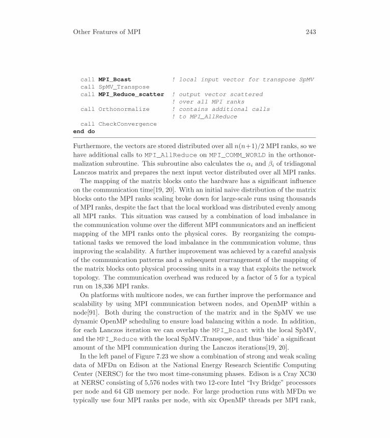
Other Features of MPI 243
call MPI_Bcast ! local input vector for transpose SpMVcall SpMV_Transposecall MPI_Reduce_scatter ! output vector scattered
! over all MPI rankscall Orthonormalize ! contains additional calls
! to MPI_AllReducecall CheckConvergence
end do
Furthermore, the vectors are stored distributed over all n(n+1)/2 MPI ranks, so we
have additional calls to MPI_AllReduce on MPI_COMM_WORLD in the orthonor-
malization subroutine. This subroutine also calculates the αi and βi of tridiagonal
Lanczos matrix and prepares the next input vector distributed over all MPI ranks.
The mapping of the matrix blocks onto the hardware has a significant influence
on the communication time[19, 20]. With an initial naive distribution of the matrix
blocks onto the MPI ranks scaling broke down for large-scale runs using thousands
of MPI ranks, despite the fact that the local workload was distributed evenly among
all MPI ranks. This situation was caused by a combination of load imbalance in
the communication volume over the different MPI communicators and an inefficient
mapping of the MPI ranks onto the physical cores. By reorganizing the compu-
tational tasks we removed the load imbalance in the communication volume, thus
improving the scalability. A further improvement was achieved by a careful analysis
of the communication patterns and a subsequent rearrangement of the mapping of
the matrix blocks onto physical processing units in a way that exploits the network
topology. The communication overhead was reduced by a factor of 5 for a typical
run on 18,336 MPI ranks.
On platforms with multicore nodes, we can further improve the performance and
scalability by using MPI communication between nodes, and OpenMP within a
node[91]. Both during the construction of the matrix and in the SpMV we use
dynamic OpenMP scheduling to ensure load balancing within a node. In addition,
for each Lanczos iteration we can overlap the MPI_Bcast with the local SpMV,
and the MPI_Reduce with the local SpMV Transpose, and thus ‘hide’ a significant
amount of the MPI communication during the Lanczos iterations[19, 20].
In the left panel of Figure 7.23 we show a combination of strong and weak scaling
data of MFDn on Edison at the National Energy Research Scientific Computing
Center (NERSC) for the two most time-consuming phases. Edison is a Cray XC30
at NERSC consisting of 5,576 nodes with two 12-core Intel “Ivy Bridge” processors
per node and 64 GB memory per node. For large production runs with MFDn we
typically use four MPI ranks per node, with six OpenMP threads per MPI rank,

244 Chapter 7
�� ����������������
�
�
��
��
��
��
����
�������
������
����
����������
�"����#�������$������#��%�������#���������$����#���#����
�������������
� � � � � ��
�
�
�
�
�
��
&�'�
���� ��������(�������)����������(&
���� ��*�������(��������)����������(&
�)(����&�������������'�(��� �!"����!���+�&��)(�)���&
Figure 7.23: Strong and weak scaling on Edison at NERSC (left) and strongscaling for two different problem sizes on Jaguar at ORNL (right, adapted fromRef. [90]) using the hybrid MPI/OpenMP implementation
although for relatively small runs (less than a few thousand cores) our MPI-only
implementation performs better. Since the workload is largely proportional to the
number of nonzero matrix elements, we show the CPU time divided by the number
of nonzero matrix elements. Perfect scaling corresponds to a straight horizontal
line. We also achieve good scaling on the leadership computing facilities at Argonne
National Laboratory and at Oak Ridge National Laboratory (ORNL): on Jaguar
(Cray XK6) at ORNL we have demonstrated 90% efficiency in strong scaling from
30,624 cores to 261,120 cores (see the right panel of Figure 7.23) using two MPI
ranks per node, with eight OpenMP threads per MPI rank.
8 Understanding How MPI Implementations Work
Understanding how MPI may be implemented can provide greater insight into the
particular design choices made by the MPI Forum. Looking at the implementation
reveals the motivation for some of the MPI design decisions. This motivation
might be missed if one considered the library design only from the viewpoint of
programmer convenience and failed to take into account the interface between the
MPI library and the underlying message-passing hardware. In this chapter, we will
briefly discuss one possible implementation approach for an MPI implementation
that sends messages between computers connected by a network.
The approach taken for the implementation here separates the complicated part
of an MPI implementation (managing communicators, derived datatypes, topolo-
gies, etc.) from the part that makes contact with the communication device. The
upper layers can remain open and independent of a particular communication de-
vice, while the communication part can be optimized for a particular device and
environment.
A more detailed and specific description of the design of several MPI implemen-
tations can be found in the literature. The MPICH implementation is described in
more detail in [57, 59]. Several projects have developed variations on the MPICH
implementation [96, 30], and many vendors, including Microsoft, Intel, IBM, and
Cray, have based their own implementations on MPICH.
We emphasize that it is impossible to say “how MPI is implemented.” It is
possible only to discuss how a particular implementation of MPI works.
8.1 Introduction
To show how an MPI implementation might work, we will start by considering
how an MPI_Send might be implemented and follow the message to the matching
MPI_Recv. Along the way, we will discover that we will need to add features to
our design.
8.1.1 Sending Data
When MPI sends data, it must include with the buffer that the user is sending
information on the message tag, communicator, length, and source and destination
of the message. We will call this additional information the envelope. Sending a
message consists of sending the envelope, followed by the data. This method of
sending the data immediately is called an eager protocol.

246 Chapter 8
8.1.2 Receiving Data
When a message arrives, there are two possible cases. Either a matching re-
ceive (e.g., MPI_Recv, MPI_Irecv, MPI_Sendrecv) has already been made or
it hasn’t. Where a matching receive already exists, the receive provides a location
for the data that is arriving behind the envelope. To keep track of what receives
are available (particularly for the nonblocking varieties), the MPI implementation
can maintain a queue1 of receives that have been posted. We can think of this as
a queue of messages that are expected, and we call it the expected queue. When
an incoming message matches a receive in this queue, the receive is marked as
completed and is removed from the queue.
Where no matching receive exists, the situation is more complicated. The re-
ceiving process must remember that a message has arrived, and it must store the
data somewhere. Let us look at these two requirements. The first requirement, to
remember that a message has arrived but has not matched a receive, is relatively
easy to handle. We keep a queue (in the same sense as the expected messages are
in a queue) of messages that were unexpected. When a program tries to receive a
message with MPI_Recv, it first checks this unexpected queue to see whether the
message has already arrived. If it has, the receive can remove the message and data
from that queue and complete. What about the data? The receiving process must
store the data somewhere. Here we have a problem. What if the message is too big
to fit in the available memory space? This situation can happen, for example, if in
a manager-worker algorithm such as the one described in Section 3.6, many workers
send large messages (say, 100 MB each) to the manager at nearly the same time.
The MPI standard requires the implementation to handle this case and not to fail.
This is the reason that we discussed buffering in Chapter 4; no matter how much
memory space is provided for unexpected messages, at some point the receiver can
run out.
8.1.3 Rendezvous Protocol
To solve the problem of delivering too much data to the destination, we need to
control how much data arrives at the destination and when that data is delivered.
One simple solution is to send only the envelope to the destination process. When
the receiver wants the data (and has a place to put the data), it sends back to the
sender a message that says, in effect, “send the data for this message now.” The
1Strictly speaking, it isn’t exactly a queue, since we don’t always take the top element off ofit. But it is ordered in the sense that if two messages have the same source, communicator, andmessage tag, the first to arrive is the first to be removed from the queue.
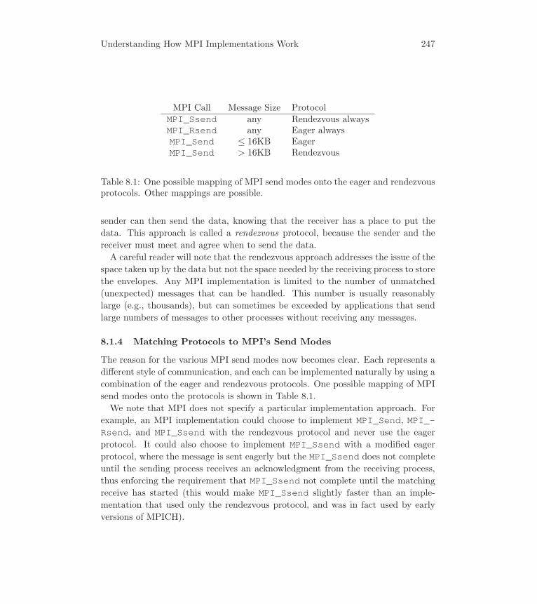
Understanding How MPI Implementations Work 247
MPI Call Message Size ProtocolMPI_Ssend any Rendezvous alwaysMPI_Rsend any Eager alwaysMPI_Send ≤ 16KB EagerMPI_Send > 16KB Rendezvous
Table 8.1: One possible mapping of MPI send modes onto the eager and rendezvousprotocols. Other mappings are possible.
sender can then send the data, knowing that the receiver has a place to put the
data. This approach is called a rendezvous protocol, because the sender and the
receiver must meet and agree when to send the data.
A careful reader will note that the rendezvous approach addresses the issue of the
space taken up by the data but not the space needed by the receiving process to store
the envelopes. Any MPI implementation is limited to the number of unmatched
(unexpected) messages that can be handled. This number is usually reasonably
large (e.g., thousands), but can sometimes be exceeded by applications that send
large numbers of messages to other processes without receiving any messages.
8.1.4 Matching Protocols to MPI’s Send Modes
The reason for the various MPI send modes now becomes clear. Each represents a
different style of communication, and each can be implemented naturally by using a
combination of the eager and rendezvous protocols. One possible mapping of MPI
send modes onto the protocols is shown in Table 8.1.
We note that MPI does not specify a particular implementation approach. For
example, an MPI implementation could choose to implement MPI_Send, MPI_-Rsend, and MPI_Ssend with the rendezvous protocol and never use the eager
protocol. It could also choose to implement MPI_Ssend with a modified eager
protocol, where the message is sent eagerly but the MPI_Ssend does not complete
until the sending process receives an acknowledgment from the receiving process,
thus enforcing the requirement that MPI_Ssend not complete until the matching
receive has started (this would make MPI_Ssend slightly faster than an imple-
mentation that used only the rendezvous protocol, and was in fact used by early
versions of MPICH).
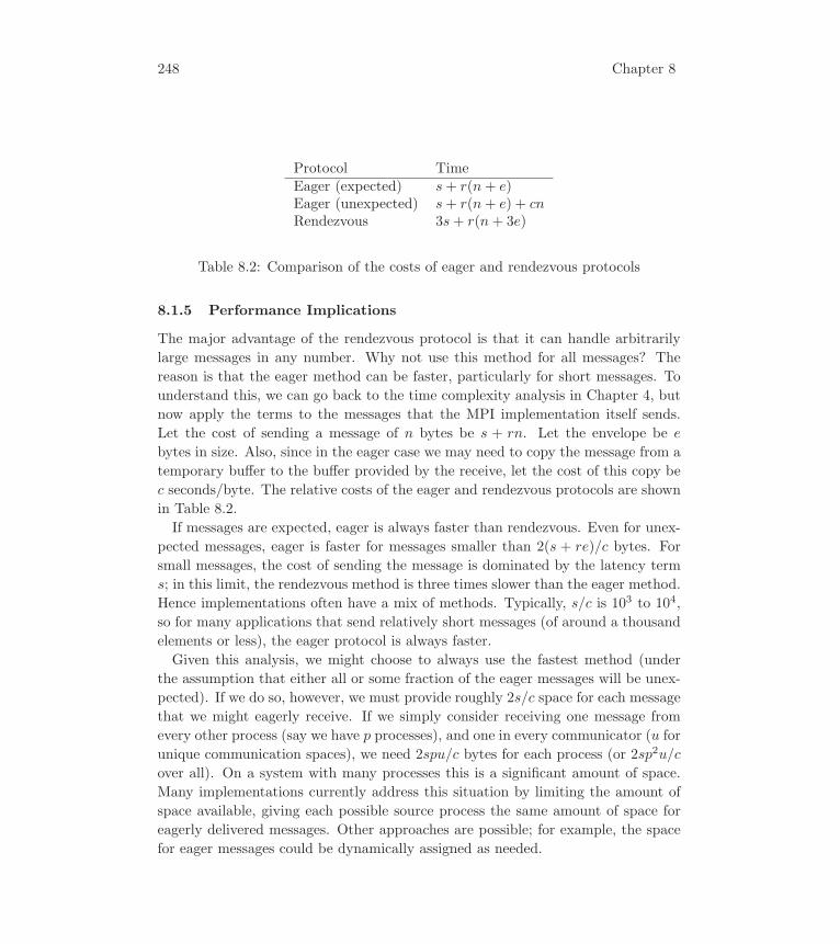
248 Chapter 8
Protocol TimeEager (expected) s+ r(n+ e)Eager (unexpected) s+ r(n+ e) + cnRendezvous 3s+ r(n+ 3e)
Table 8.2: Comparison of the costs of eager and rendezvous protocols
8.1.5 Performance Implications
The major advantage of the rendezvous protocol is that it can handle arbitrarily
large messages in any number. Why not use this method for all messages? The
reason is that the eager method can be faster, particularly for short messages. To
understand this, we can go back to the time complexity analysis in Chapter 4, but
now apply the terms to the messages that the MPI implementation itself sends.
Let the cost of sending a message of n bytes be s + rn. Let the envelope be e
bytes in size. Also, since in the eager case we may need to copy the message from a
temporary buffer to the buffer provided by the receive, let the cost of this copy be
c seconds/byte. The relative costs of the eager and rendezvous protocols are shown
in Table 8.2.
If messages are expected, eager is always faster than rendezvous. Even for unex-
pected messages, eager is faster for messages smaller than 2(s + re)/c bytes. For
small messages, the cost of sending the message is dominated by the latency term
s; in this limit, the rendezvous method is three times slower than the eager method.
Hence implementations often have a mix of methods. Typically, s/c is 103 to 104,
so for many applications that send relatively short messages (of around a thousand
elements or less), the eager protocol is always faster.
Given this analysis, we might choose to always use the fastest method (under
the assumption that either all or some fraction of the eager messages will be unex-
pected). If we do so, however, we must provide roughly 2s/c space for each message
that we might eagerly receive. If we simply consider receiving one message from
every other process (say we have p processes), and one in every communicator (u for
unique communication spaces), we need 2spu/c bytes for each process (or 2sp2u/c
over all). On a system with many processes this is a significant amount of space.
Many implementations currently address this situation by limiting the amount of
space available, giving each possible source process the same amount of space for
eagerly delivered messages. Other approaches are possible; for example, the space
for eager messages could be dynamically assigned as needed.
Understanding How MPI Implementations Work 249
8.1.6 Alternative MPI Implementation Strategies
Here we have briefly sketched one implementation approach. There are others. For
example, it is possible for a receive to send a message to the source of the message
(when MPI_ANY_SOURCE is not used) indicating that a message is expected [98].
This can reduce the latency introduced by the rendezvous protocol by eliminating
one message exchange. Other approaches can be used when the hardware sup-
ports remote memory access or some form of shared memory. For example, most
MPI implementations support networks with hardware support for remote memory
operations and make use of shared memory for communication within a node.
8.1.7 Tuning MPI Implementations
Most MPI implementations provides some parameters to allow MPI users to tune
the performance for their applications. From the preceding discussion, we know
that both the amount of space available for eager delivery of messages and the
message size at which an MPI_Send or MPI_Isend switches from eager to ren-
dezvous protocol are natural parameters, and many MPI implementations allow
the user some control over these. For example, the MPICH implementation has
an environment variable MPICH_CVAR_EAGER_LIMIT that sets the message size
above which the rendezvous protocol is used. Note, however, that you can’t just
set this to 4000000000; there is usually a range of valid values.
These parameters are implementation-dependent and can change with time. Each
vendor’s documentation for MPI should be checked to see what environment vari-
ables are available.
In some cases, there are options that you may want to use during program devel-
opment. For example, some implementations, including MPICH, allow the user to
control the level of error checking and reporting. Once a program has been thor-
oughly debugged, turning off these checks can save time, particularly in latency-
sensitive parts of the application. MPI-3 added a standard way to discover and
modify these values, which are called control variables . These are discussed in
Using Advanced MPI [55], Chapter 9.
8.2 How Difficult Is MPI to Implement?
MPI has many functions. How difficult is it to implement all of these functions?
How difficult is it to develop a high-performance MPI implementation? MPI was
carefully designed so that the features of MPI are orthogonal, allowing an imple-
mentation both to build a full MPI implementation on top of a smaller number

250 Chapter 8
of routines and to incrementally improve the implementation by replacing parts of
the MPI implementation with more sophisticated techniques as the implementation
matures.
This is a common approach. For example, in graphics and printing, most graph-
ical displays provide for drawing a single pixel at an arbitrary location. Any other
graphical function can be built by using this single, elegant primitive. However,
high-performance graphical displays offer a wide variety of additional functions,
ranging from block copy and line drawing to 3-D surface shading. MPI imple-
mentations tend to follow this same approach: at the very bottom of the MPI
implementation are routines to communicate data between processes. An MPI
implementation, early in its life, may implement all of MPI in terms of these oper-
ations. As time goes on, it can add more advanced features. For example, special
routines to provide faster collective operations might exploit special features of the
parallel computer’s hardware. The topology routines (i.e., MPI_Cart_create and
MPI_Graph_create) can become aware of the parallel computer’s interconnect
topology.
One example of a feature in MPI that implementations are improving incremen-
tally is the handling of MPI’s derived datatypes. Early implementations of MPI
often did the equivalent of using MPI_Pack followed by a send of contiguous data.
As implementations have matured, they have addressed the issue of providing better
performance on MPI derived datatypes; see [61], for example.
8.3 Device Capabilities and the MPI Library Definition
Earlier we commented that considering the device interface illuminates some of the
design decisions in MPI. Any message-passing library imposes a certain view of
the characteristics of the devices it is intended for. MPI was carefully designed to
impose as few restrictions as possible, thus allowing implementations that take full
advantage of modern, powerful communications hardware.
For a simple example, consider the case of MPI_Probe, the blocking “probe”
function. Recall that MPI also has a nonblocking version, MPI_Iprobe. Not all
message-passing libraries support probe at all, and those that do tend to supply
only the nonblocking version, since the blocking one can be implemented at the
user level by calling the nonblocking one in a loop. However, this “busy waiting” is
not really acceptable in a multithreaded or even multiprogramming environment.
If the library supplies the blocking probe as well, then the implementation can use
whatever resources it may have, such as an intelligent communication controller, to
free the CPU while waiting for a message.

Understanding How MPI Implementations Work 251
Similarly, from the programmer’s point of view there is no need for the (block-
ing) function MPI_Recv, since its functionality can be obtained with MPI_Irecvfollowed by MPI_Wait. On the other hand, the library can make more efficient use
of the device if it does not have to return to the user halfway through the operation.
Another case in point is the use of a datatype parameter on all MPI communica-
tion calls, rather than using MPI_Pack and MPI_Unpack together with sending
untyped data. Explicit packing and unpacking, while sometimes necessary, forces
a memory copy operation that usually is not.
Other parts of the MPI library, such as MPI_Waitany, clearly could be imple-
mented at the user level and thus are not necessary in order for the programmer to
implement an algorithm. Eliminating them would make MPI a smaller and simpler
library. On the other hand, it would also eliminate opportunities for optimization
by the communications layer. One reason that MPI is a relatively large library is
that the MPI Forum deliberately sacrificed the notion of a “minimalist” library in
favor of enabling high performance.
8.4 Reliability of Data Transfer
The MPI standard specifies that the message-passing operations are reliable. This
means that the application programmer who uses a correct implementation of MPI
need not worry about whether the data sent has been delivered correctly. However,
it does mean that the MPI implementation must take steps to ensure that messages
are delivered reliably.
No mechanism for delivering data is 100% reliable. Even direct, memory-to-
memory interconnects have a small probability of failure. This is what parity and
ECC (error correcting code) memories and data paths are for. Parity allows errors
to be detected, ECC allows some (usually single-bit) errors to be corrected and
others (usually double-bit) detected. In the case of more loosely connected systems,
the probability of an uncorrectable failure is higher.
For example, take the commonly used network protocol TCP. This protocol pro-
vides reliable data connections between two points. But what does “reliable” mean
in this context? It turns out that since 100% reliability is impossible, any TCP
implementation must be prepared to decide that a connection has failed. At that
point, TCP terminates the connection and reliably notifies the users of the connec-
tion that the connection has been closed. This is the meaning of “reliable” in TCP:
data is delivered, or it is possible to discover that something went wrong.
This level of reliability is adequate in some circumstances but not in others. Many
of the MPI Forum participants intended for MPI to provide what is often called

252 Chapter 8
“guaranteed delivery”: MPI is expected to ensure that the message is delivered,
correcting for any errors that may occur in the lower-level data-movement layers.
In the TCP case, this might mean keeping track of how much data has been suc-
cessfully delivered and, if a connection fails, having MPI automatically re-establish
the connection and continue sending the data. However, being able to ensure that
data has been delivered adds extra overhead and can reduce the performance of
MPI (or any other message-passing or data-delivery system).

9 Comparing MPI with Sockets
In this chapter, we will discuss just one other system for interprocess communication
in detail. This system is sockets, which is a common, low-level mechanism for
communicating between different computers. Sockets is widely available; modern
scripting languages such as Python make it easy to program with sockets.
The socket application programmer interface (API) is the basic programming
interface for using TCP (among other methods) to send data between processes
that are connected by many networks, including the Internet. The details of this
interface are not covered here; see, for example, [115] for detailed coverage of the
use of sockets. In this discussion we focus on using TCP with sockets. We will cover
only a subset of the socket interface that illuminates the differences from MPI and
similarities with it.
Sockets are used primarily to establish a point-to-point communication path be-
tween two processes. Once a connection is established between two processes (using
socket, bind, listen, accept, and connect), the two processes have file de-
scriptors (fds) with which they can read from and write to the socket. At the
simplest level, a read on a socket is similar to an MPI_Recv, and a write on
a socket is similar to an MPI_Send. However, the differences between MPI and
sockets are interesting.
Let us look first at how data can be sent with sockets. In the case of sockets, a
write call can return with a positive value, indicating that that number of bytes
were written, or a negative value, indicating a problem (and no bytes written). The
behavior of read is similar: the returned value indicates the number of bytes read,
with an negative value indicating a problem (and no bytes read).
For sockets, as for MPI, the handling of message buffers is key to understanding
what happens. The first part to note is that an attempt to write count bytes to
the socket may be only partially successful. What happens depends on whether the
socket has been set to be nonblocking (with the flag O_NONBLOCK or O_NDELAYset using the fcntl call on the sockets file descriptor). If the socket has not been
set as nonblocking, then the write will succeed; that is, it will return with value
count as long as count is no larger than the size of the socket buffer (this also
assumes that the socket buffer is empty, for example, when no data has yet been
sent on the socket). If count is greater than the socket size, then the write call
will block until enough data has been read from the other end of the socket. In this
mode, a write is like an MPI_Send: small enough data buffers are sent even if
no receive is waiting for them, while sending (writing) larger data buffers can block
the process, waiting for a receive to occur at the other end of the communication.
For the same reasons that we discussed in Chapter 4, it can be difficult in some

254 Chapter 9
void Sender(int fd, char *buf, int count){
int n;while (count > 0) {
n = write(fd, buf, count);if (n < 0) { ... special handling ... }count -= n;buf += n;
}}
void Receiver(int fd, char *buf, int count){
int n;while (count > 0) {
n = read(fd, buf, count);if (n < 0) { ... special handling ... }count -= n;buf += n;
}}
Figure 9.1: Partial code to send data between two processes
cases to guarantee that a program using write and read won’t deadlock because
two processes are both trying to write data to a socket that is already full of data.
To avoid this problem, a socket can be marked as nonblocking. In this case, the
behavior of read and write are different from the blocking case. For write, ifthere is no room for the data, the write call returns the value -1 and sets errnoto EAGAIN.1 This keeps the process from blocking but requires the programmer
to take other steps to deliver the data. For example, when a write fails, the
programmer might try to read from the socket, in the event that the socket is
being written to from both ends (the “unsafe” case of each process executing a
write to the other, intending to follow that with a read). In this mode, write and
read are somewhat like MPI_Isend and MPI_Irecv, but with a different way of
handling MPI_Wait. Note that this nonblocking mode for sockets is provided to
allow applications to function correctly in the presence of limited buffering, just as
for the MPI nonblocking modes.
1In a multithreaded environment, you must access the per-thread value of errno.

Comparing MPI with Sockets 255
Some operating systems provide asynchronous read and write operations, called
aio_read and aio_write, respectively. These are an alternative interface for
nonblocking read and write operations and are closer to the MPI nonblocking op-
erations in spirit. Note, however, that there is no requirement in MPI (or in the
definitions of aio_read or aio_write for that matter) that these operations
take place concurrently with computation.
Continuing the analogy with the MPI nonblocking operations, the socket API
provides its own counterpart to MPI_Waitsome and MPI_Testsome. These are
the select and poll calls, whose arguments are file descriptor masks. Selectand poll can return immediately, in analogy with MPI_Testsome (when called
with a timeout value of zero), or block until at least one of the fds is ready to be
read from or written to. The difference is that select and poll only indicate
that a file descriptor may be used; in MPI, a successful test or wait completes the
related communication. A sketch of what an implementation of MPI_Testsomemight look like in an implementation that communicates over sockets is shown in
Figure 9.2.
9.1 Process Startup and Shutdown
When describing a message-passing library or application, most of the time is spent
discussing the mechanisms for sending data between processes. This overlooks the
difficulty in simply getting the processes started, particularly in a scalable way. To
illustrate the issues, we will briefly describe some of the possibilities.
Starting a parallel job consists of two steps: starting the processes and putting
those processes in contact with one another. Different approaches may be taken for
each of these steps.
One of the simplest approaches is for the first process, for example, the single
process that is started by mpiexec, to start all the other processes by using a
remote shell program such as rsh or ssh. This initial process is called the manager
process. In this approach, a command-line argument can be used to give the new
processes the port number of a socket on the first process that can be connected to
in order to get information on all of the processes in the MPI job.
This approach has the advantage of making use of existing facilities for starting
processes and for routing standard in, out, and error. The disadvantages are many.
For example, it is not scalable (all processes are connected to the manager process)
and it relies on remote shell (considered a security risk) or a secure variant. In
environments where a process manager is used for load balancing, this approach
cannot be used because only the process manager is allowed to start tasks.
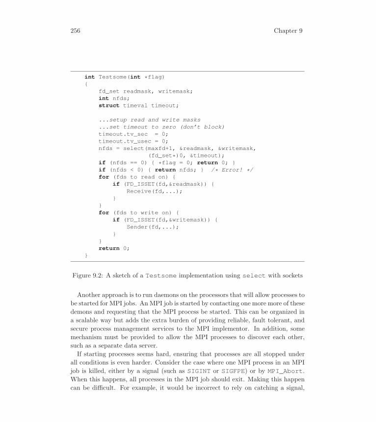
256 Chapter 9
int Testsome(int *flag){
fd_set readmask, writemask;int nfds;struct timeval timeout;
...setup read and write masks
...set timeout to zero (don’t block)timeout.tv_sec = 0;timeout.tv_usec = 0;nfds = select(maxfd+1, &readmask, &writemask,
(fd_set*)0, &timeout);if (nfds == 0) { *flag = 0; return 0; }if (nfds < 0) { return nfds; } /* Error! */for (fds to read on) {
if (FD_ISSET(fd,&readmask)) {Receive(fd,...);
}}for (fds to write on) {
if (FD_ISSET(fd,&writemask)) {Sender(fd,...);
}}return 0;
}
Figure 9.2: A sketch of a Testsome implementation using select with sockets
Another approach is to run daemons on the processors that will allow processes to
be started for MPI jobs. An MPI job is started by contacting one more more of these
demons and requesting that the MPI process be started. This can be organized in
a scalable way but adds the extra burden of providing reliable, fault tolerant, and
secure process management services to the MPI implementor. In addition, some
mechanism must be provided to allow the MPI processes to discover each other,
such as a separate data server.
If starting processes seems hard, ensuring that processes are all stopped under
all conditions is even harder. Consider the case where one MPI process in an MPI
job is killed, either by a signal (such as SIGINT or SIGFPE) or by MPI_Abort.When this happens, all processes in the MPI job should exit. Making this happen
can be difficult. For example, it would be incorrect to rely on catching a signal,
Comparing MPI with Sockets 257
since some Unix signals are uncatchable (e.g., SIGKILL and SIGSTOP). Similarly,
relying on a “watchdog” process is also unreliable, since the watchdog itself may
fail or be killed (for example, some operating systems will kill processes when the
OS starts to run short of critical resources like swap space; this might happen as a
result of a runaway parallel program, thus causing the OS to kill the one process,
the watchdog, that could save the day).
9.2 Handling Faults
The MPI standard says little about what happens when something goes wrong. The
reason is largely that standards rarely specify the behavior of erroneous programs
or the consequences of events beyond the standard (such as a power failure). This is
a good match to highly scalable systems where communication between processes is
guaranteed by the underlying operating environment and where scalable and high-
performance implementation of the MPI collective routines is important. However,
in a more loosely coupled network environment, such as a collection of workstations,
there is much greater likelihood that contact with another process will be lost, and
applications written using sockets often include code to handle this event.
One reason that this is easier to handle in the socket case than it is in the MPI
case is that there are only two parties to the socket: if one fails, then it is reasonably
clear what needs to be done. In the case of MPI, the failure of one process among
a thousand during an MPI collective operation such as an MPI_Allreduce makes
it difficult to recover (one can ensure that the MPI_Allreduce operation succeeds
for all members of the communicator before allowing the MPI program to continue,
but only at a significant performance cost).
An MPI implementation could provide the same level of support for commu-
nication failures in the case of communicators of size two; this is a “quality of
implementation” issue. That is, there is no reason why an MPI implementation
cannot provide the same level of support for failures in communication as sockets
as long as only two-party communicators are used. A generalization of this, to
intercommunicators where the two “parties” are the groups of processes, can also
be made [58].
The MPI Forum has been discussing for several years extensions of MPI to provide
greater support for fault tolerance. While the general idea seems simple, the details
are surprisingly difficult. One difficult constraint is that many users of MPI depend
on MPI providing the highest possible performance; these users are often unwilling
to sacrifice any performance for fault tolerance. Proving that a feature will not

258 Chapter 9
impact the performance of any current or future MPI implementation is nearly
impossible.
Perhaps more important, the nature of the faults that MPI is expected to survive
has a major impact on the fault tolerance features that are needed. Most of the
work to date on MPI fault tolerance has focused on surviving the failure of a process.
However, the failure of a process almost always results in data being lost by the
computation, making it impossible to continue without additional steps being taken
by the application to recover that data. For extreme-scale systems, a more common
fault may be a transient memory error—one that causes incorrect data to be stored
but does not cause the process to fail. More work is needed before a useful and
effective fault-tolerant extension to MPI can be defined. This is an active area of
research, with many projects and results. For more information, see, for example,
[58, 44, 45, 40, 72, 122, 83, 33, 30].
10 Wait! There’s More!
MPI is a standard library (and notation) specification for supporting the message-
passing model of parallel computation. The MPI Forum interpreted its mission
broadly (not without considerable discussion), and “message passing” in MPI in-
cludes not only many varieties of point-to-point communication but also contexts,
groups, collective operations, process topologies, and profiling and environmen-
tal inquiry functions. Making MPI a large specification widened the scope of its
applicability.
10.1 Beyond MPI-1
As soon as the MPI-1 standard was released, however, it was seen that the ideas
behind MPI could be applied more widely, to the benefit of applications. Work on
extending MPI took on three overall directions:
• Generalizing the fixed nature of MPI_COMM_WORLD. The MPI (-1) pro-
cess model described in this book assumes that the number of processes par-
ticipating in the parallel computation is fixed before the program begins. A
more dynamic approach is to allow a computation to create new processes
during the run or to establish MPI communication with processes already
running in a separate MPI_COMM_WORLD.
• Generalizing the notion of message passing. The idea here is to explore
ways that a process can cause events to occur on another process or processor
without sending a message that the other process must explicitly receive, such
as a remote signal or remote memory copy.
• Generalizing the notion of computation. As parallel machines have be-
come larger, many applications based on scalable algorithms for their core
computations have seen their bottlenecks shift from computation and inter-
process communication to input and output of data. New parallel computers
have parallel hardware in the file system, but what a “parallel file” means or
what parallel I/O should be in general is still an open research question.
These and other topics were taken up by the MPI-2 and MPI-3 Forums and from
the subject matter of the companion volume to this one, Using Advanced MPI [55].

260 Chapter 10
10.2 Using Advanced MPI
In the present volume, you have been introduced to the basic concepts of MPI
and seen how to apply them in a diverse set of concrete programming situations.
The subset of the MPI standard presented here is sufficient for implementing quite
large and sophisticated application programs, as demonstrated by the application
examples appearing in several chapters.
The companion volume, Using Advanced MPI [55], continues the tutorial ap-
proach we have used so far into the parts of the current MPI standard that em-
body the extensions to basic MPI that we enumerated in the previous section. In
particular, Using Advanced MPI covers the following topics.
Large scale systems. When MPI was first defined, an MPI program with 100
ranks was a highly parallel program. Now, applications with millions of ranks
are running on the world’s largest machines. The MPI-3 Forum in particular
has introduced features into the standard that address the issues of scalabil-
ity that arise both in the interface itself and its implementation. Particular
enhancements include nonblocking and neighborhood collective operations.
Remote memory access. Introduced in MPI-2, remote memory access (or one-
sided operations) were substantially extended and refined by the MPI-3 Fo-
rum.
Using shared memory. Nearly all today’s machines have the capability of hav-
ing multiple processes (with separate MPI ranks) share memory on a node
of the machine. MPI-3 introduced functionality to allow programming this
configuration with MPI.
Hybrid programming. Although we did touch on hybrid programming with
OpenMP and MPI in this book, Using Advanced MPI contains a much deeper
discussion of the issues surrounding multithreaded programming with MPI
and new MPI-3 functionality in support of it.
Parallel I/O. The MPI-2 Forum introduced the MPI approach to parallel I/O,
in which the analogy of sending/receiving messages to writing/reading files is
exploited through the use of non-blocking and collective operations, together
with the use of MPI datatypes to describe noncontiguous, typed data, both
in memory and in files.
Coping with large data. Current data sizes dwarf those envisioned at the time
of MPI-1 and MPI-2. Strategies for dealing with this issue are discussed.

Wait! There’s More! 261
Performance and correctness debugging. MPI-3 introduced a new tools in-
terface that has the potential to provide substantially more capability that
the profiling interface presented in this book. Other debugging approaches
are also described.
Dynamic process management. MPI-2 introduced the notion that a set of MPI
processes could create a new set of MPI processes. This functionality is only
starting to be used by applications.
Working with modern Fortran. In this book, our appendix has described some
issues presented by the Fortran interface. These issues are explored more
deeply in Using Advanced MPI, particularly the use of the mpi_f08 module.
Features for libraries. MPI-2 and MPI-3 introduced a number of features to
further support the development of MPI-based libraries. These are described
in Using Advanced MPI.
10.3 Will There Be an MPI-4?
MPI-2 introduced a lot of new, sophisticated technology into MPI, and it took a
surprising amount of time before high-performance implementations were available.
MPI-3 introduced fewer new features into MPI, but some, such as the reworked
one-sided communication interface, are likely to take time to implement well. Ex-
perience will need to be gained with applications and with mature implementations
of MPI-3 in order to fully understand where MPI needs to be extended. Topics
under discussion include fault tolerance, extensions to two-sided message passing,
and a tighter integration with thread-based programming models.
10.4 Beyond Message Passing Altogether
Message passing is not the only approach to parallel computing, and other ap-
proaches have been suggested. The first is called PGAS (for Partitioned Global
Address Space) languages. The idea of these languages is to enable programming
with essentially a shared-memory model (load/store) but with an awareness of the
performance implications of local vs. remote access. These are compiler-based,
rather than library-based, approaches. The C version of this approach is UPC [14]
and the Fortran version is Co-Array Fortran (CAF) [2, 3], and is part of the Fortran
2008 standard. There is also a Java version called Titanium [13]. UPC and CAF
are installed on a number of today’s largest machines.

262 Chapter 10
The PGAS languages retain the MPI feature that the programmer is directing
the behavior of a specific number of processes. In what we might call the HPCS
languages (since they were developed as part of DARPA’s High-Productivity Com-
puting Systems project) this restriction is relaxed. Only the parallelism itself is
specified; how it is executed is left to the implementation. The HPCS languages
are Chapel [1], X10 [15], and Fortress [4].
10.5 Final Words
When we wrote the first edition of this book, we never thought that we would be
doing a third edition some twenty years later. Yet the MPI Forum focus, constant
over the years, on functionality, portability, and performance, leaving “user con-
venience” to library writers, has proved to be a robust framework indicating that
MPI will be an essential component of large, small, current, and future systems.
We hope that this introduction to MPI will provide you with the understanding
you will need as parallel computing confronts the future.
Glossary of Selected Terms
The following is a glossary of the most commonly used terms in this book. While
it is far from complete, it does provide a number of useful definitions in one place.
Active Messages An active message is normally a short message that causes re-
mote execution on the receiving process of a specified section of code while
delivering to that code the active-message “payload.” Analogous to remote
procedure calls used in most Unix/Linux/POSIX systems, the active-message
paradigm is a means both for implementing higher-level protocols like MPI
and for direct programming in certain situations. Active messages are an
extension to the message-passing model of MPI.
Application Programmer Interface (API) An application programmer inter-
face (API) is the set of callable functions (or methods used with objects, or
both), and rules and guidelines for how one software library (or component)
will work with or contract with another. A library (or component) is often
said to publish its API. In practical terms, an API provides a set of capabil-
ities and rules that, when used correctly, provide services and operations to
an application programmer. Operating systems publish APIs of system calls
(POSIX is one such example, Win32 another). MPI has a standardized API
(the main topic of this book), which consists of its function calls, parameters,
arguments, and rules for accomplishing group-oriented message passing. APIs
can have versions, a good example of which is that MPI started from MPI-1,
which has been updated over the past twenty years to MPI-2 and MPI-3; now
MPI-4 is being developed.
Application Topology Application topologies are the natural process intercon-
nection implied by the algorithm, in parallel. MPI supports the mapping
of application topologies onto virtual topologies, and virtual topologies onto
physical hardware topologies.
Attributes Attributes in MPI are integers (in Fortran) or pointers (in C) that can
be attached, by key value, to a communicator.
Asynchronous Communication Asynchronous communication is often used in-
terchangeably with nonblocking communication. This is generally communi-
cation in which the sender and receiver place no constraints on each other
in terms of completion and which may also overlap as much as possible with
computation. The term asynchronous communication is not used in MPI.

264 Glossary
Bandwidth The bandwidth of a message transmission is its transfer rate. Band-
width is the reciprocal of the time needed to transfer a byte (the incremental
per-byte cost).
Blocking Communication Blocking communication refers to communication in
which the call does not complete (or return control to the calling program)
until the buffer is available for reuse (in the case of the send) or use (in the
case of a receive). See Blocking Send and Blocking Receive.
Blocking Receive A blocking receive is a receive that blocks until the data buffer
contains the selected message. See Nonblocking Receive.
Blocking Send A blocking send is a send that blocks until the data buffer is avail-
able for reuse. This may or may not require recipient to begin the process of
receiving the message. The details of the blocking depend on the implemen-
tation and the amount of buffering that the system may choose to do or be
able to do.
Buffered Communication Communication in which the send operation (which
may be blocking or nonblocking) may make use of a user-provided buffer, in
order to ensure that the send does not block (and possibly deadlock) while
waiting for space to store the user’s message. This is primarily of use with
blocking sends, where this mode removes the possibility that the matching
receive may need to start before the blocking, buffered send call can return.
Buffering may involve additional copying of data and can impact performance.
Buffering Buffering refers to the amount or act of copying (or the amount of
memory) that the system uses as part of its transmission protocols. Generally,
buffering helps avoid deadlocks, making programming easier for specific cases
but less portable and predictable.
Caching of Attributes Caching is the process of attaching attributes in MPI to
a communicator. See Attributes.
Cartesian Topology Cartesian topology is the type of virtual topology that sup-
ports regular mapping of processes into an N-dimensional name space. Ex-
amples include two- and three-dimensional logical process topologies used for
linear algebra and PDE computations.
Collective Communication Collective communication involves operations such
as “broadcast” (MPI_Bcast) and “all reduce” (MPI_Allreduce) that in-

Glossary 265
volve the entire group of a communicator, rather than just two members, as
in point-to-point communication.
Communication Modes MPI provides buffered, ready, standard, and synchron-
ous communication modes for point-to-point communication.
Communication Processor A communication processor is generally the hard-
ware component that provides the local access of a processor to the paral-
lel computer network. Such processors are also called “router chips” and
“mesh-routing chips” or MRCs on some systems. As time passes, the com-
munication processor and its “glue chips” are becoming capable of more than
simple transfers to and from CPUs, and may be capable of “gather/scatter”-
type operations and other high-speed memory accesses without direct CPU
intervention.
Communicator A communicator is a group of processes plus the notion of safe
communication context. MPI has two types of communicators: intracom-
municators (the default), and intercommunicators (these involve two disjoint
groups of processes). Communicators guarantee that communication is iso-
lated from other communication in the system and also that collective com-
munication is isolated from point-to-point communication. Some people think
of communicators as “virtual fabrics” of communication.
Context In MPI, the context is not a user-visible quantity per se but is the internal
mechanism by which a communicator endows a group with safe communica-
tion space, separating such communication from all others in the system and
separating point-to-point and collective communication of a communicator’s
group.
Contiguous Data The simplest message buffers consist of data that is not dis-
persed in memory but, rather, is contiguous. MPI deals with this case, and
with more general noncontiguous data, through datatypes. An example of
contiguous data would be ten double precision numbers starting at a base
address, and stored consecutively in memory.
Datatypes The MPI objects that support general gather and scatter of complex
data specifications are called datatypes. The simple ones are built in, and
user-defined data types are called derived datatypes.
266 Glossary
Deadlock The state of execution where the computation cannot proceed because
an impasse is reached where two or more processes depend directly or indi-
rectly on each other for a result before continuing. A good example is two
processes trying to receive from each other, then send to each other, in a
blocking communication mode.
Deprecated Function A deprecated function or feature of MPI is one that has
been replaced by a better way of performing the same operation in a later
version of the standard. Switching to using the “new way” is recommended.
Deprecated functions will eventually be removed from future versions of the
standard.
Erroneous Program An erroneous program in MPI standard terminology is one
that uses MPI in a way that is invalid according to the standard. Such
programs have undetermined behavior. In some cases, erroneous programs
actually run. Compare with Unsafe Programs, which is another category of
MPI program.
Event An event is the unit of logging for program instrumentation. Events are
considered to have no duration.
Fault Tolerance Fault tolerance is a feature of a program or library such as MPI
that allows it to detect, mitigate, isolate, and potentially recover from a
misbehavior (a fault, leading in turn to a failure) of hardware and/or soft-
ware. MPI’s standardized model has assumed reliable underlying hardware
and lower-level software up to now, but a number of “fault tolerant MPIs”
have been proposed and prototyped over the past 15 years.
GPGPU General-purpose computing on graphical processing units (GPGPUs),
which are typically combined with a conventional processor and programmed
with a special purpose language such as CUDA, OpenACC, or OpenCL.
Graph Topology Graph topology is the type of virtual topology that allows gen-
eral relationships between processes, where processes are represented by nodes
of a graph.
Group A group (or process group) is an ordered collection of processes. Each
process has a rank in the group. The rank runs from zero to one less than
the number of processes.
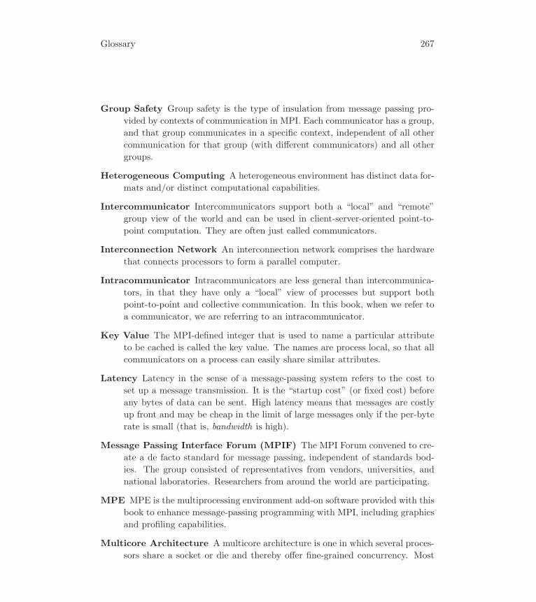
Glossary 267
Group Safety Group safety is the type of insulation from message passing pro-
vided by contexts of communication in MPI. Each communicator has a group,
and that group communicates in a specific context, independent of all other
communication for that group (with different communicators) and all other
groups.
Heterogeneous Computing A heterogeneous environment has distinct data for-
mats and/or distinct computational capabilities.
Intercommunicator Intercommunicators support both a “local” and “remote”
group view of the world and can be used in client-server-oriented point-to-
point computation. They are often just called communicators.
Interconnection Network An interconnection network comprises the hardware
that connects processors to form a parallel computer.
Intracommunicator Intracommunicators are less general than intercommunica-
tors, in that they have only a “local” view of processes but support both
point-to-point and collective communication. In this book, when we refer to
a communicator, we are referring to an intracommunicator.
Key Value The MPI-defined integer that is used to name a particular attribute
to be cached is called the key value. The names are process local, so that all
communicators on a process can easily share similar attributes.
Latency Latency in the sense of a message-passing system refers to the cost to
set up a message transmission. It is the “startup cost” (or fixed cost) before
any bytes of data can be sent. High latency means that messages are costly
up front and may be cheap in the limit of large messages only if the per-byte
rate is small (that is, bandwidth is high).
Message Passing Interface Forum (MPIF) The MPI Forum convened to cre-
ate a de facto standard for message passing, independent of standards bod-
ies. The group consisted of representatives from vendors, universities, and
national laboratories. Researchers from around the world are participating.
MPE MPE is the multiprocessing environment add-on software provided with this
book to enhance message-passing programming with MPI, including graphics
and profiling capabilities.
Multicore Architecture A multicore architecture is one in which several proces-
sors share a socket or die and thereby offer fine-grained concurrency. Most

268 Glossary
processors produced today (even for laptops and embedded devices) offer
multiple cores. A multicore architecture is a kind of multiprocessor.
Multiprocessor A multiprocessor refers to a single computer with multiple pro-
cessors sharing memory and other resources. Originally implemented with
multiple processors and a shared-memory network, or on a single computer
with a shared bus, multiprocessors now include the nearly ubiquitous multi-
core architecture.
Node Node is used in two senses in this book. In one sense, it is synonymous with
processor; in the other, it refers to the nodes of a graph, which is a standard
computer science data structure.
Nonblocking Communication In a nonblocking communication, the call does
not wait for the communication to be completed. See NonBlocking Receive
and NonBlocking Send.
Nonblocking Receive A non-blocking receive is a receive operation that may
return before the data buffer contains an incoming message. This is often
used to provide the location and layout of the data buffer to the lower-level
message passing hardware in order to provide better performance.
Nonblocking Send The send may return before the data buffer is available for re-
use. The intent is that the send returns almost immediately. A nonblocking
send must not require a matching receive to start before returning.
Overlapping of Communication, Computation, I/O In some systems, asyn-
chronous communication, computation, and input-output can be overlapped
in time, so that the total time is shorter than if each of these operations was
done sequentially. MPI supports the potential for overlapping of communica-
tion and computation with its nonblocking operations, although implemen-
tations and underlying hardware vary in their ability to support this kind of
concurrency. When it works on a system, overlapping can hide some of the
cost of message passing.
Pairwise Ordering The pairwise ordering property of message-passing systems
is essential to the message-passing programming paradigm of MPI and its
ancestor systems. This property guarantees that two messages sent between
a pair of processes arrives in the order they were sent. With the introduction
of “contexts,” this requirement is weakened to require that two messages sent
between a pair of processes using the same communicator arrive in the same

Glossary 269
order they were sent. MPI does weaken this further by changing the order of
messages of different tags between the same processor pair.
Parallel Library A library is an “encapsulation” of an algorithm in a way that is
meant to be convenient for multiple uses in a single application and/or reuse
in multiple applications. Library writers for parallel computers can build
robust libraries because MPI specifically provides features to help libraries to
isolate their communication from that of users and other libraries.
Persistent Requests Persistent requests are used when multiple communications
are to be started, tested, or completed, in order to reduce costs and provide
the user with access to higher performance.
Physical Topology Physical topology is the topology of the parallel computer
interconnection network, such as a mesh or hypercube.
Point-to-Point Communication Point-to-point communication is between two
members of a communicator; (generically, a send-receive type call).
Portability Portability is the concept of moving a program from one environment
to another. The degree of portability indicates the amount of work needed
to get the program to run again. High-quality portability (also called perfor-
mance portability, or transportability) implies that reasonable performance
is retained as a product of that porting process. MPI is designed to help
ensure that high performance is possible across a number of different parallel
platforms.
Process A process is the smallest addressable unit of computation in the MPI
model. A process resides on a processor (or node). MPI does not discuss how
processes are born, die, or are otherwise managed.
Processor A processor is (loosely) the CPU, memory, and I/O capabilities of a
subset of a parallel machine (or a workstation in a workstation cluster). A
processor supports the execution of one or more processes in the MPI model,
but MPI makes only limited connection between processes and processors in
environmental inquiry routines and in two topology-related mapping routines.
Quiescence The quiescence property requires that programmers guarantee that
no outside communication will impinge on a group of processes during a
specific period of execution, in order for a given operation to execute correctly.
Quiescence demands that no pending point-to-point communication is in place
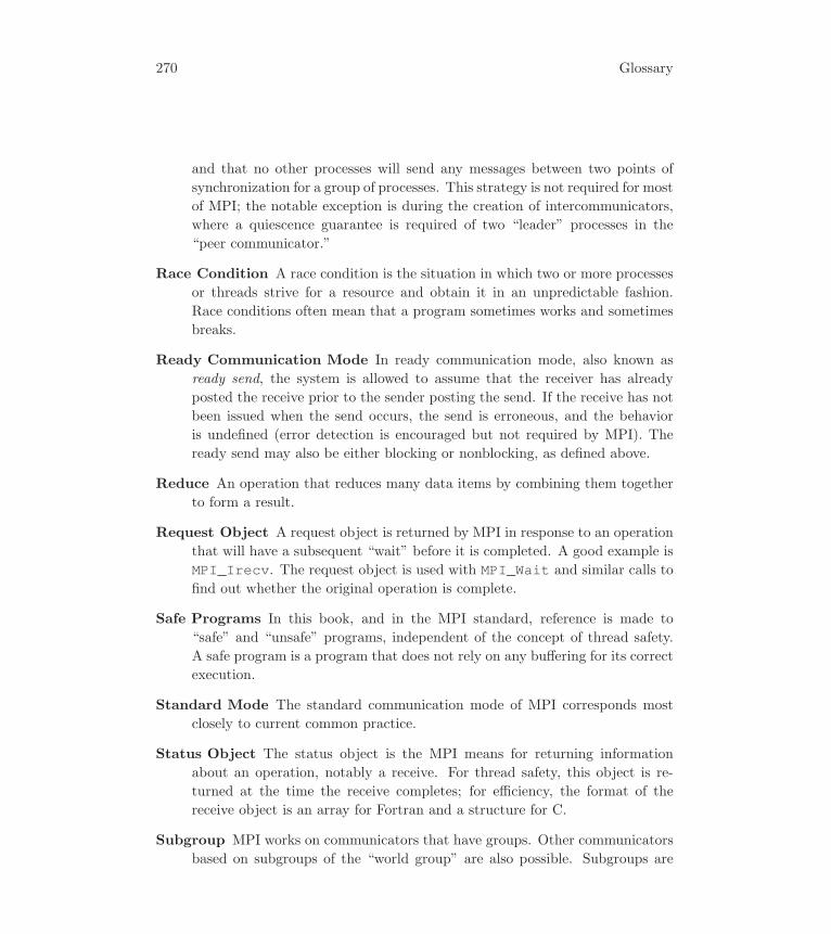
270 Glossary
and that no other processes will send any messages between two points of
synchronization for a group of processes. This strategy is not required for most
of MPI; the notable exception is during the creation of intercommunicators,
where a quiescence guarantee is required of two “leader” processes in the
“peer communicator.”
Race Condition A race condition is the situation in which two or more processes
or threads strive for a resource and obtain it in an unpredictable fashion.
Race conditions often mean that a program sometimes works and sometimes
breaks.
Ready Communication Mode In ready communication mode, also known as
ready send, the system is allowed to assume that the receiver has already
posted the receive prior to the sender posting the send. If the receive has not
been issued when the send occurs, the send is erroneous, and the behavior
is undefined (error detection is encouraged but not required by MPI). The
ready send may also be either blocking or nonblocking, as defined above.
Reduce An operation that reduces many data items by combining them together
to form a result.
Request Object A request object is returned by MPI in response to an operation
that will have a subsequent “wait” before it is completed. A good example is
MPI_Irecv. The request object is used with MPI_Wait and similar calls to
find out whether the original operation is complete.
Safe Programs In this book, and in the MPI standard, reference is made to
“safe” and “unsafe” programs, independent of the concept of thread safety.
A safe program is a program that does not rely on any buffering for its correct
execution.
Standard Mode The standard communication mode of MPI corresponds most
closely to current common practice.
Status Object The status object is the MPI means for returning information
about an operation, notably a receive. For thread safety, this object is re-
turned at the time the receive completes; for efficiency, the format of the
receive object is an array for Fortran and a structure for C.
Subgroup MPI works on communicators that have groups. Other communicators
based on subgroups of the “world group” are also possible. Subgroups are

Glossary 271
just as flexible as groups from which they are defined, and no distinction is
necessary, except that it is convenient to call certain groups “subgroups” and
certain communicators “subcommunicators” when describing algorithms.
Synchronization Synchronization is an operation that forces a group of processes
all to pass through a critical section of code before any can continue. Many
MPI collective operations are potentially synchronizations, but not all are re-
quired to be implemented with this property (except MPI_Barrier, whichis specifically designed to be a synchronization). See also Synchronous Com-
munication Mode.
Synchronous Communication Mode The sender in the synchronous commu-
nication mode may not return until the matching receive has been issued
on the destination process. Synchronous sends may be either blocking or
nonblocking, depending on whether the data buffer provided to the send is
available for reuse when the send call returns.
Thread A thread is the atomic notion of execution within an MPI process. Each
MPI process has a main thread and may have additional threads, provided
a thread-safe programming environment and threads package are both avail-
able. The MPI interface is thread safe but does not tie MPI specifically to
any thread paradigm or standard. Implementations of MPI may or may not
be thread safe. The precise level of thread safety offered in an MPI imple-
mentation can be found in an MPI program with functions introduced in
MPI-2.
Thread Safety Thread safety is the quality of software semantics that guarantees
that independently executing threads will not interfere with each other by
accessing data intended for a different thread. Implementing thread safety
requires eliminating most global state and explicitly managing use of any
global state that cannot be eliminated. MPI is designed to be a thread-
safe specification. Implementations may or may not achieve thread safety
internally.
Topology See Virtual Topology.
Type Map A type map is the sequence of pairs of basic MPI datatypes and dis-
placements that make up, in part, a derived datatype.
Type Signature The type signature is the MPI concept that extracts just the
sequence of datatypes from a type map.

272 Glossary
Unsafe Program In MPI, a program is called unsafe if it depends on resources
or an implementation to work in a particular way that is not mandated, such
as that there be internal buffering of a certain size. Unsafe programs can
work correctly on some systems, and fail on others, or even change char-
acteristics for different length messages or for different versions on an MPI
implementation. An example is two MPI ranks both sending each other a
blocking message, which can result in deadlock ; however, the program might
run OK on a specific MPI implementation that buffers data internally. Such
a program is said to be unsafe but not erroneous.
User-Defined Topology If MPI’s virtual topologies are insufficient, then users
can easily build their own topologies. Such topologies are often application-
oriented.
Virtual Topology Virtual topologies are a naming of processes in a communica-
tor other than the rank naming. Graphs, Cartesian grids, and user-defined ar-
rangements are all possible. Virtual topologies link applications more closely
to communicators because the names of processes reflect the communication
pattern needed for it. See also Application Topology.

A The MPE Multiprocessing Environment
Here we describe the MPE library that has been used in the examples throughout
this book. It consists of functions that are
• consistent in style with MPI,
• not in MPI,
• freely available, and
• will work with any MPI implementation.
These tools are rudimentary and lack many desirable features. Nonetheless, we
have found them useful in the preparation of this book.
The files ‘mpe.h’ and ‘mpef.h’ should be included for C and Fortran programs,
respectively.
A.1 MPE Logging
The C bindings for the logging routines are given in Table A.1 and the Fortran
bindings in Table A.2.
These routines allow the user to log events that are meaningful for specific appli-
cations, rather than relying on automatic logging of MPI library calls. The basic
routines are MPE_Init_log, MPE_Log_event, and MPE_Finish_log. MPE_-Init_log must be called (by all processes) to initialize MPE logging data struc-
tures. MPE_Finish_log collects the log data from all the processes, merges it,
and aligns the timestamps with respect to the times at which MPE_Init_log and
MPE_Finish_log were called. Then, the process with rank 0 in MPI_COMM_-WORLD writes the log into the file whose name is given as an argument. A single
event is logged with the MPE_Log_event routine, which specifies an event type
(completely up to the user), and one integer and one character string for user data.
In order to place in the logfile data that might be useful for a logfile analysis or
visualization program (like jumpshot), the routines MPE_Describe_event and
MPE_Describe_state allow one to add event and state descriptions and to de-
fine states by specifying a starting and ending event for each state. One can also
suggest a state color to be used by the logfile visualizations program. In the case
of jumpshot, the color can be of the form “red:vlines” in order to specify si-
multaneously a color for a color display and a bitmap for black-and-white displays
(such as books).

274 Appendix A
int MPE Init log(void)
int MPE Start log(void)
int MPE Stop log(void)
int MPE Finish log(char *logfilename)
int MPE Describe state(int start, int end, char *name, char *color)
int MPE Describe event(int event, char *name)
int MPE Log event(int event, int intdata, char *chardata)
Table A.1: C bindings for MPE logging routines
MPE INIT LOG()
MPE FINISH LOG(logfilename)
character*(*) logfilename
MPE START LOG()
MPE STOP LOG()
MPE DESCRIBE STATE(start, end, name, color)integer start, endcharacter*(*) name, color
MPE DESCRIBE EVENT(event, name)integer eventcharacter*(*) name
MPE LOG EVENT(event, intdata, chardata)integer event, intdatacharacter*(*) chardata
Table A.2: Fortran bindings for MPE logging
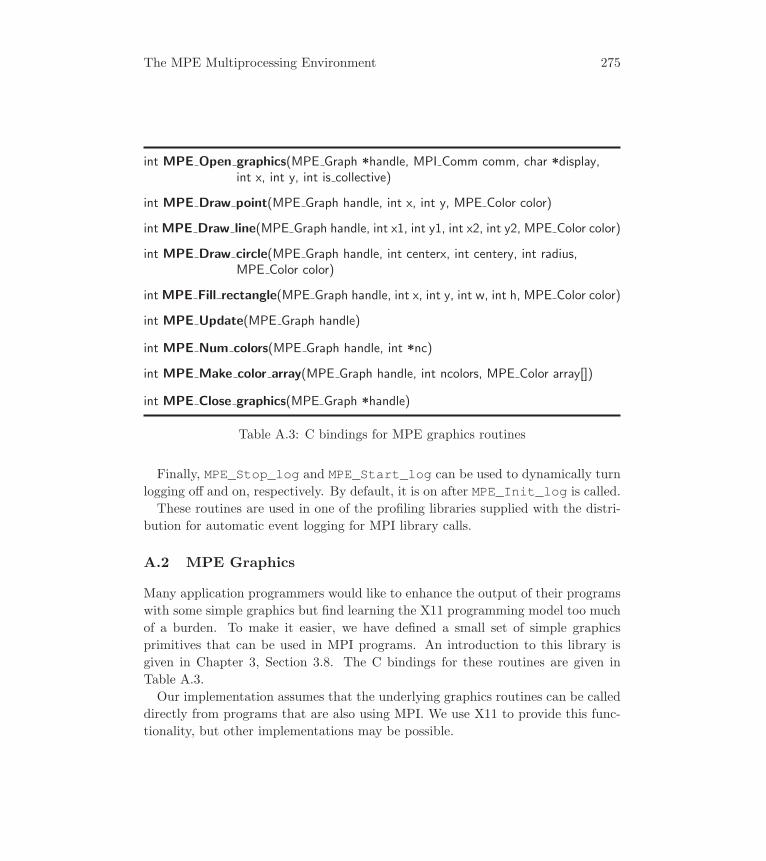
The MPE Multiprocessing Environment 275
int MPE Open graphics(MPE Graph *handle, MPI Comm comm, char *display,int x, int y, int is collective)
int MPE Draw point(MPE Graph handle, int x, int y, MPE Color color)
intMPE Draw line(MPE Graph handle, int x1, int y1, int x2, int y2, MPE Color color)
int MPE Draw circle(MPE Graph handle, int centerx, int centery, int radius,MPE Color color)
int MPE Fill rectangle(MPE Graph handle, int x, int y, int w, int h, MPE Color color)
int MPE Update(MPE Graph handle)
int MPE Num colors(MPE Graph handle, int *nc)
int MPE Make color array(MPE Graph handle, int ncolors, MPE Color array[])
int MPE Close graphics(MPE Graph *handle)
Table A.3: C bindings for MPE graphics routines
Finally, MPE_Stop_log and MPE_Start_log can be used to dynamically turn
logging off and on, respectively. By default, it is on after MPE_Init_log is called.
These routines are used in one of the profiling libraries supplied with the distri-
bution for automatic event logging for MPI library calls.
A.2 MPE Graphics
Many application programmers would like to enhance the output of their programs
with some simple graphics but find learning the X11 programming model too much
of a burden. To make it easier, we have defined a small set of simple graphics
primitives that can be used in MPI programs. An introduction to this library is
given in Chapter 3, Section 3.8. The C bindings for these routines are given in
Table A.3.
Our implementation assumes that the underlying graphics routines can be called
directly from programs that are also using MPI. We use X11 to provide this func-
tionality, but other implementations may be possible.

276 Appendix A
MPE OPEN GRAPHICS(handle, comm, display, x, y,is collective, ierror)integer handle, comm, x, y, ierrorcharacter*(*) displaylogical is collective
MPE DRAW POINT(handle, x, y, color, ierror)integer handle, x, y,color, ierror
MPE DRAW LINE(handle, x1, y1, x2, y2, color, ierror)integer handle, x1, y1, x2, y2, color, ierror
MPE DRAW CIRCLE(handle, centerx, centery, radius, color,ierror)integer handle, centerx, centery, radius, color, ierror
MPE FILL RECTANGLE(handle, x, y, w, h, color, ierror)integer handle, x, y, w, h, color, ierror
MPE UPDATE(handle, ierror)integer handle, ierror
MPE NUM COLORS(handle, nc, ierror)integer handle, nc, ierror
MPE MAKE COLOR ARRAY(handle, ncolors, array, ierror)
integer handle, ncolors, array(*), ierror
MPE CLOSE GRAPHICS(handle, ierror)integer handle, ierror
Table A.4: Fortran bindings for MPE graphics routines
A.3 MPE Helpers
In addition to the logging and graphics code, the MPE library contains a number
of routines to aid programmers in producing parallel applications. The routine
MPE_Decomp1d was used in Chapter 4 to compute decompositions of an array.
The routines MPE_Counter_create, MPE_Counter_free, MPE_Counter_-nxtval, and MPE_Counter_service were defined in Chapter 7 to implement a
remote counter. Bindings for these routines are shown in Tables A.5 and A.6.
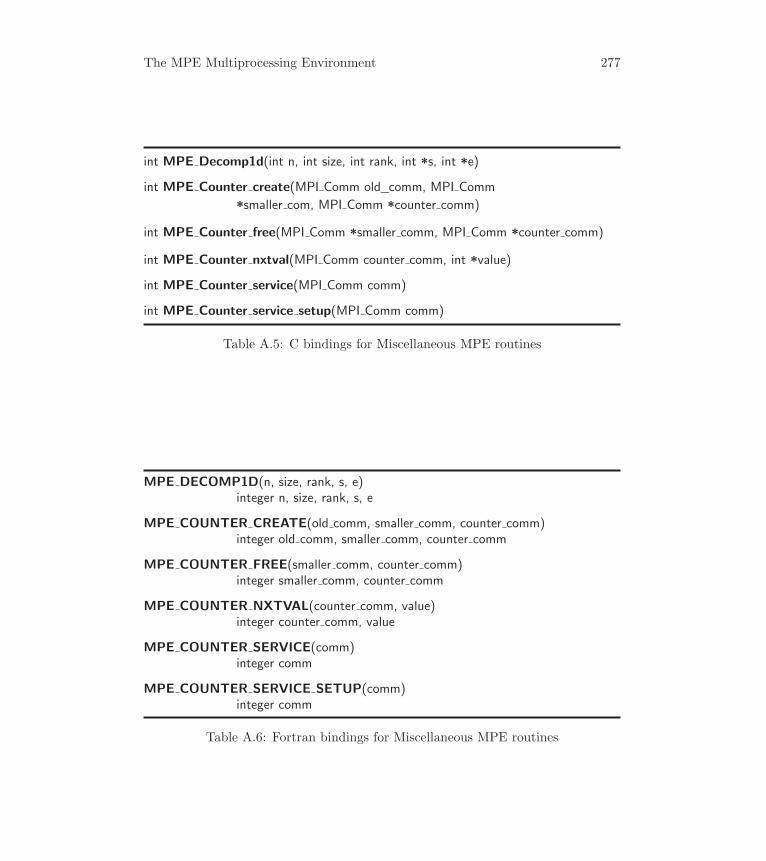
The MPE Multiprocessing Environment 277
int MPE Decomp1d(int n, int size, int rank, int *s, int *e)
int MPE Counter create(MPI Comm old_comm, MPI Comm
*smaller com, MPI Comm *counter comm)
int MPE Counter free(MPI Comm *smaller comm, MPI Comm *counter comm)
int MPE Counter nxtval(MPI Comm counter comm, int *value)
int MPE Counter service(MPI Comm comm)
int MPE Counter service setup(MPI Comm comm)
Table A.5: C bindings for Miscellaneous MPE routines
MPE DECOMP1D(n, size, rank, s, e)integer n, size, rank, s, e
MPE COUNTER CREATE(old comm, smaller comm, counter comm)integer old comm, smaller comm, counter comm
MPE COUNTER FREE(smaller comm, counter comm)integer smaller comm, counter comm
MPE COUNTER NXTVAL(counter comm, value)integer counter comm, value
MPE COUNTER SERVICE(comm)integer comm
MPE COUNTER SERVICE SETUP(comm)integer comm
Table A.6: Fortran bindings for Miscellaneous MPE routines

B MPI Resources Online
Here we describe how to get access to MPI-related material on the Internet.
Examples of MPI programs. All the examples used in this book are available
on the web at http://www.mcs.anl.gov/mpi/usingmpi. The file ‘README’lists the files by chapter. A Unix ‘tar’ file (compressed) containing all of the
examples is available in ‘examples.tar.gz’. Instructions for unpacking this file
are in the ‘README’ file. In addition, any errata items for this book will be made
available at that web site.
MPI implementations. The MPICH implementation, written by the authors of
this book and others, is freely available and may be downloaded at http://www.mpich.org. The MPICH implementation includes examples and test programs.
Most of the test programs may be used with any MPI implementation.
The MPI standard. The MPI standard is available in PDF at http://www.mpi-forum.org. Errata for MPI-1, MPI-2, and MPI-3 are also available there.
A great deal of information on parallel programming projects and tools is avail-
able on the net. We encourage you to investigate other sites for other resources on
MPI and parallel computing.

C Language Details
In this appendix we briefly discuss some details of C and Fortran that interact with
MPI.
C.1 Arrays in C and Fortran
This section discusses the layout of C and Fortran arrays in memory and talks
briefly about how implicit “reshapes” of arrays are handled in Fortran. All arrays
are stored in memory according to some rule, defined by the language, that says how
to map the indices of an array reference such as a(i,j,k,l) into a computer’s
memory. Understanding and exploiting this rule are important in creating efficient
representations of data.
C.1.1 Column and Row Major Ordering
Many discussions of the differences between Fortran and C arrays refer to “column”
and “row” major ordering. These terms come from looking at a two-dimensional
array as representing a matrix. To understand this, consider the m× n matrix
⎛⎜⎜⎝
a11 a12 a13 · · · a1na21 a22 a23 · · · a2n...
......
......
am1 am2 am3 · · · amn
⎞⎟⎟⎠
If we use the Fortran declaration
real a(m,n)
and represent the matrix element aij with a(i,j), then column major ordering,
used in the Fortran language, means that the elements are stored by columns; that
is, they are stored in the order a(1,1), a(2,1), ..., a(m,1), a(1,2),..., a(m,n). Row major ordering, used in the C language, means that the
elements are stored by rows; that is, a[0][0], a[0][1], ..., a[0][n-1],a[1][0], ..., a[m-1][n-1]. We have used Fortran and C array notation
here to emphasize how each is stored in memory.
C.1.2 Meshes vs. Matrices
While a matrix-based view of arrays is common and often helpful, a different view of
arrays is more natural for many applications, for instance, the 2-D Poisson example
in Chapter 4. The solution to the problem had a natural representation as a function

282 Appendix C
u(x, y). We solved this problem on a discrete mesh of points (xi, yj) and used the
Fortran element u(i,j) to represent u(xi, yj). While this approach seems entirely
natural, consider how this appears:
u(1,m) u(2,m) · · · u(n,m)u(1,m-1) u(2,m-1) · · · u(n,m-1)
......
......
u(1,1) u(2,1) · · · u(n,1)
Viewed this way, the rows are stored together! What is going on?
The real story is that Fortran arrays are (always) stored so that, when we look
at how the elements are placed in memory, we see that the first index varies most
rapidly. In fact, the rule for mapping a Fortran array into memory is simple: If
the array is declared as A(N1,N2,...), then A(I1,I2,...) is the (I1-1) +N1*((I2-1) + N2*(...))th element (starting from zero).
The rule for C is the opposite; the last index varies most rapidly. When consid-
ering the special case of two dimensions and looking at the arrays as representing
matrices, we see how these lead to the row- and column-major interpretations.
C.1.3 Higher Dimensional Arrays
Once we know how arrays are laid out in the computer’s memory, we can use that
information to design ways to access sections of multidimensional arrays, planes
with one coordinate constant, for example. If we wish to send a plane of data
out of a 3-D array, we can form three different datatypes, one for each coordinate
direction.
For concreteness, consider a Fortran array dimensioned as
double precision a(nx,ny,nz)
We will consider two different situations. In the first, we wish to send an entire
face of this 3-D rectangular array. In the second, we wish to send only a rectangular
part of the face. We will see that exploiting the knowledge of how data is laid out in
memory will allow us to use a single MPI_Type_vector call for the first situation,
while in the second situation (involving a part of a face) we will need to build a
derived type from another derived type.
This is a good place to mention that most MPI implementations do not un-
derstand Fortran array sections. That is, you should not pass a part of an array
using, for example, a(3:10,19:27,4). Instead, you should pass the first element
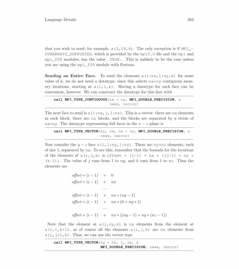
Language Details 283
that you wish to send; for example, a(3,19,4). The only exception is if MPI_-SUBARRAYS_SUPPORTED, which is provided by the mpif.h file and the mpi and
mpi_f08 modules, has the value .TRUE.. This is unlikely to be the case unless
you are using the mpi_f08 module with Fortran.
Sending an Entire Face. To send the elements a(1:nx,1:ny,k) for some
value of k, we do not need a datatype, since this selects nx*ny contiguous mem-
ory locations, starting at a(1,1,k). Having a datatype for each face can be
convenient, however. We can construct the datatype for this face with
call MPI_TYPE_CONTIGUOUS(nx * ny, MPI_DOUBLE_PRECISION, &newz, ierror)
The next face to send is a(1:nx,j,1:nz). This is a vector: there are nx elements
in each block, there are nz blocks, and the blocks are separated by a stride of
nx*ny. The datatype representing full faces in the x− z plane is
call MPI_TYPE_VECTOR(nz, nx, nx * ny, MPI_DOUBLE_PRECISION, &newy, ierror)
Now consider the y − z face a(i,1:ny,1:nz). There are ny*nz elements, each
of size 1, separated by nx. To see this, remember that the formula for the locations
of the elements of a(i,j,k) is offset + (i-1) + nx * ((j-1) + ny *(k-1)). The value of j runs from 1 to ny, and k runs from 1 to nz. Thus the
elements are
offset+ (i− 1) + 0
offset+ (i− 1) + nx
· · ·offset+ (i− 1) + nx ∗ (ny − 1)
offset+ (i− 1) + nx ∗ (0 + ny ∗ 1)· · ·
offset+ (i− 1) + nx ∗ ((ny − 1) + ny ∗ (nz − 1))
Note that the element at a(i,ny,k) is nx elements from the element at
a(i,1,k+1), as of course all the elements a(i,j,k) are nx elements from
a(i,j+1,k). Thus, we can use the vector type
call MPI_TYPE_VECTOR(ny * nz, 1, nx, &MPI_DOUBLE_PRECISION, newx, ierror)

284 Appendix C
These examples show the power of the blockcount argument in the MPI vector
datatype creation calls.
Sending a Partial Face. If instead of sending the entire face of the cube, we
want to send or receive the elements a(sx:ex,sy:ey,k) for some value of k, wecan define a vector datatype newz:
call MPI_TYPE_VECTOR(ey-sy+1, ex-sx+1, nx, &MPI_DOUBLE_PRECISION, newz, ierror)
call MPI_TYPE_COMMIT(newz, ierror)call MPI_SEND(a(sx,sy,k), 1, newz, dest, tag, comm, ierror)
To understand this, we need only look at the discussion of arrays above. For the
elements a(sx:ex,sy:ey,k), we see that the data consists of ey-sy+1 groups
(“columns”) of ex-sx+1 elements (“rows”); the rows are contiguous in memory.
The stride from one group to another (i.e., from a(sx,j,k) to a(sx,j+1,k)) isjust nx double-precision values. Note that this is an example of a vector type with
a block count that is different from one.
Similarly, to send or receive the elements a(sx:ex,j,sz:ez), we can use
call MPI_TYPE_VECTOR(ez-sz+1, ex-sx+1, nx*ny, &MPI_DOUBLE_PRECISION, newy, ierror)
call MPI_TYPE_COMMIT(newy, ierror)
The explanation is the same as for a(sx:ex,sy:ey,k) except that the stride
between elements is nx*ny double-precision values.
The final case, to send or receive the elements a(i,sy:ey,sz:ez), requires alittle more work because we cannot use the blocklength argument in MPI_Type_-vector. In this case, we take advantage of MPI’s ability to form a datatype from
an MPI datatype. First, for a datatype for the elements a(i,sy:ey,k), we use
call MPI_TYPE_VECTOR(ey-sy+1, 1, nx, &MPI_DOUBLE_PRECISION, newx1, ierror)
(We do not need to commit newx1 because we will not be using it in a com-
munication operation.) Next, we form a vector of these types. Since the stride
between these elements is probably not an integral multiple of ey-sy+1, we use
MPI_Type_create_hvector; this routine measures the stride in bytes.
call MPI_TYPE_SIZE(MPI_DOUBLE_PRECISION, sizeof, ierror)stride = nx*ny*sizeofcall MPI_TYPE_CREATE_HVECTOR(ez-sz+1, 1, stride, &
newx1, newx, ierror)

Language Details 285
call MPI_TYPE_COMMIT(newx, ierror)
An approach similar to that in Section 5.4 can be used to generate more general
datatypes.
C.2 Aliasing
MPI routines such as MPI_Allreduce have both input and output buffers. It
might seem natural to use code like this:
sum = ...call MPI_ALLREDUCE(sum, sum, 1, MPI_INTEGER, MPI_SUM, &
MPI_COMM_WORLD, ierr)
This code is incorrect; we mentioned in Section 3.1 that the input and output buffers
had to be distinct (nonoverlapping). This is a requirement of Fortran of which some
programmers are not aware. The Fortran standard states that if an actual argument
is repeated, then the routine may not assign a value to it. Repeating an argument
is called aliasing . This prohibits the form of use of the MPI_Allreduce call given
above, because the second use of the repeated argument sum has a value assigned
to it by the routine. For consistency, the C versions of the MPI routines share this
restriction (even though the C language does not prohibit aliasing).
In MPI-2, this restriction was eased somewhat. Many of the collective routines al-
low the use of the value MPI_IN_PLACE as the value of the sendbuf or recvbuf.For example, MPI_Allreduce allows MPI_IN_PLACE as the sendbuf argument.
In that case, the input data is taken from recvbuf. MPI_IN_PLACE is discussed
in Section 5.2.1 in the MPI-3 standard [94].

References
[1] Chapel home page. chapel.cray.com.
[2] Co-Array Fortran. co-array.org.
[3] Co-Array Fortran at Rice University. caf.rice.edu.
[4] Fortress. https://projectfortress.java.net.
[5] HPL – A Portable Implementation of the High-performance Linpack Bench-
mark for Distributed-memory Computers. http://www.netlib.org/hpl.
[6] InfiniBand R© Trade Association. http://www.infinibandta.org.
[7] LAPACK – Linear Algebra PACKage. http://www.netlib.org/lapack.
[8] ParMETIS web page. http://glaros.dtc.umn.edu/gkhome/metis/parmetis/overview.
[9] Scalable Parallel Pseudo Random Number Generator. http://www.sprng.org.
[10] Scalasca. www.scalasca.org.
[11] The Asynchronous Dynamic Load-Balancing Library. http://svn.cs.mtsu.edu/svn/adlbm.
[12] The Trilinos Project. http://trilinos.sandia.gov.
[13] Titanium. titanium.cs.berkeley.edu.
[14] Unified Parallel C. upc.lbl.gov.
[15] X10: Performance and productivity at scale. x10-lang.org.
[16] Yarcdata. http://www.yarcdata.com.
[17] Jeanne C. Adams, Walter S. Brainerd, Jeanne T. Martin, Brian T. Smith,
and Jerrold L. Wagener. Fortran 95 Handbook. MIT Press, Cambridge, MA,
1997.

288 References
[18] L. Adhianto, S. Banerjee, M. Fagan, M. Krentel, G. Marin, J. Mellor-
Crummey, and N. R. Tallent. HPCTOOLKIT: tools for performance analysis
of optimized parallel programs. Concurrency and Computation: Practice and
Experience, 22(6):685–701, 2010.
[19] Hasan Metin Aktulga, Chao Yang, Esmond G. Ng, Pieter Maris, and James P.
Vary. Topology-aware mappings for large-scale eigenvalue problems. In Chris-
tos Kaklamanis, Theodore S. Papatheodorou, and Paul G. Spirakis, editors,
Euro-Par, volume 7484 of Lecture Notes in Computer Science, pages 830–842.
Springer, 2012.
[20] Hasan Metin Aktulga, Chao Yang, Esmond G. Ng, Pieter Maris, and James P.
Vary. Improving the scalability of a symmetric iterative eigensolver for multi-
core platforms. Concurrency and Computation: Practice and Experience,
2013.
[21] Srinivas Aluru, G. M. Prabju, and John Gustafson. A random-number gen-
erator for parallel computers. Parallel Computing, 18:839–847, 1992.
[22] Andrew W. Appel. An efficient program for many-body simulation. SIAM
Journal of Sci. and Stat. Comp., 6:85–103, January 1985.
[23] Enes Bajrovic and Jesper Larsson Traff. Using MPI derived datatypes in
numerical libraries. In Yiannis Cotronis, Anthony Danalis, Dimitrios S.
Nikolopoulos, and Jack Dongarra, editors, Recent Advances in the Message
Passing Interface - 18th European MPI Users’ Group Meeting, EuroMPI
2011, Santorini, Greece, September 18-21, 2011. Proceedings, volume 6960
of Lecture Notes in Computer Science, pages 29–38. Springer, 2011.
[24] Satish Balay, Shrirang Abhyankar, Mark F. Adams, Jed Brown, Peter Brune,
Kris Buschelman, Victor Eijkhout, William D. Gropp, Dinesh Kaushik,
Matthew G. Knepley, Lois Curfman McInnes, Karl Rupp, Barry F. Smith,
and Hong Zhang. PETSc users manual. Technical Report ANL-95/11 -
Revision 3.5, Argonne National Laboratory, 2014.
[25] B. S. Baldwin and H. Lomax. Thin-layer approximation and algebraic model
for separated turbulent flows. AIAA, January 1978. AIAA-78-257.
[26] Joshua E. Barnes and Piet Hut. A hierarchical O(N log N) force calculation
algorithm. Nature, 324(4):446–449, December 1986.
References 289
[27] A. Beguelin, J. Dongarra, G. A. Geist, R. Manchek, and V. Sunderam. A
user’s guide to PVM: Parallel virtual machine. Technical Report TM-11826,
Oak Ridge National Laboratory, Oak Ridge, TN, 1991.
[28] L. S. Blackford, J. Choi, A. Cleary, E. DAzevedo, J. Demmel, I. Dhillon,
J. Dongarra, S. Hammarling, G. Henry, A. Petitet, K. Stanley, D. Walker,
and R. C. Whaley. ScaLAPACK Users’ Guide. SIAM, Philadelphia, 1997.
[29] L. Bomans, D. Roose, and R. Hempel. The Argonne/GMD macros in FOR-
TRAN for portable parallel programming and their implementation on the
Intel iPSC/2. Parallel Computing, 15:119–132, 1990.
[30] Aurelien Bouteiller, Thomas Herault, Geraud Krawezik, Pierre Lemarinier,
and Franck Cappello. MPICH-V project: A multiprotocol automatic fault-
tolerant MPI. IJHPCA, 20(3):319–333, 2006.
[31] James Boyle, Ralph Butler, Terrence Disz, Barnett Glickfeld, Ewing Lusk,
Ross Overbeek, James Patterson, and Rick Stevens. Portable Programs for
Parallel Processors. Holt, Rinehart, and Winston, New York, NY, 1987.
[32] T. A. Brody. Random-number generation for parallel processors. Computer
Physics Communications, 56:147–153, 1989.
[33] Darius Buntinas. Scalable distributed consensus to support MPI fault toler-
ance. In Proc. IEEE International Parallel and Distributed Processing Sympo-
sium (26th IPDPS’12), pages 1240–1249, Shanghai, China, May 2012. IEEE
Computer Society.
[34] Greg Burns, Raja Daoud, and James Vaigl. LAM: An open cluster envi-
ronment for MPI. In John W. Ross, editor, Proceedings of Supercomputing
Symposium ’94, pages 379–386. University of Toronto, 1994.
[35] Ralph Butler and Ewing Lusk. User’s guide to the p4 parallel programming
system. Technical Report ANL-92/17, Argonne National Laboratory, October
1992.
[36] Ralph Butler and Ewing Lusk. Monitors, messages, and clusters: The p4
parallel programming system. Parallel Computing, 20:547–564, April 1994.
[37] N. Carriero and D. Gelernter. How to write parallel programs. ACM Com-
puting Surveys, 21(3):323–356, September 1989.

290 References
[38] Barbara Chapman, Gabriele Jost, and Ruud van der Paas. Using OpenMP:
Portable Shared Memory Parallel Programming. MIT Press, Cambridge, MA,
2008.
[39] Parasoft Corporation. Express version 1.0: A communication environment
for parallel computers, 1988.
[40] Charng da Lu and Daniel A. Reed. Assessing fault sensitivity in MPI appli-
cations. In SC, page 37. IEEE Computer Society, 2004.
[41] Eric D. Demaine. A threads-only MPI implementation for the development
of parallel programs. In Proceedings of the 11th International Symposium on
High Performance Computing Systems, pages 153–163, July 1997.
[42] J. J. Dongarra, J. DuCroz, I. Duff, and R. Hanson. A set of Level 3 basic
linear algebra subprograms. ACM Transactions on Mathematical Software,
16:1–17, March 1989.
[43] J. J. Dongarra, J. DuCroz, S. Hammarling, and R. Hanson. An extended set
of Fortran basic linear algebra subprograms. ACM Transactions on Mathe-
matical Software, 14:1–17, March 1988.
[44] Graham E. Fagg and Jack Dongarra. FT-MPI: Fault tolerant MPI, supporting
dynamic applications in a dynamic world. In Jack Dongarra, Peter Kacsuk,
and Norbert Podhorszki, editors, PVM/MPI, volume 1908 of Lecture Notes
in Computer Science, pages 346–353. Springer, 2000.
[45] Graham E. Fagg and Jack Dongarra. Building and using a fault-tolerant MPI
implementation. IJHPCA, 18(3):353–361, 2004.
[46] FFTW. http://www.fftw.org/.
[47] P.F. Fischer and J.W. Lottes. Hybrid Schwarz-multigrid methods for the
spectral element method: Extensions to Navier-Stokes. In R. Kornhuber,
R. Hoppe, J. P?riaux, O. Pironneau, O. Widlund, and J. Xu, editors, Domain
Decomposition Methods in Science and Engineering Series. Springer, Berlin,
2004.
[48] I. Foster, J. Geisler, W. Gropp, N. Karonis, E. Lusk, G. Thiruvathukal, and
S. Tuecke. A wide-area implementation of the Message Passing Interface.
Parallel Computing, 24(12):1735–1749, 1998.

References 291
[49] I. Foster, W. Gropp, and R. Stevens. The parallel scalability of the spectral
transform method. Monthly Weather Review, 120(5):835–850, 1992.
[50] I. Foster and C. Kesselman, editors. The Grid: Blueprint for a Future Com-
puting Infrastructure. Morgan Kaufmann Publishers, 1999.
[51] Geoffrey C. Fox, Mark A. Johnson, Gregory A. Lyzenga, Steve W. Otto,
John K. Salmon, and David W. Walker. Solving Problems on Concurrent
Processors, volume 1. Prentice Hall, 1988.
[52] G. A. Geist, M. T. Heath, B. W. Peyton, and P. H. Worley. PICL: A portable
instrumented communications library, C reference manual. Technical Report
TM-11130, Oak Ridge National Laboratory, Oak Ridge, TN, July 1990. See
also http://www.epm.ornl.gov/picl.
[53] John R. Gilbert and Robert Schreiber. Optimal data placement for dis-
tributed memory architectures. In Parallel Processing for Scientific Comput-
ing, pages 462–471. SIAM, March 1991.
[54] Leslie Greengard. The Rapid Evaluation of Potential Fields in Particle Sys-
tems. ACM Press, New York, NY, 1987.
[55] William Gropp, Torsten Hoefler, Rajeev Thakur, and Ewing Lusk. Using Ad-
vanced MPI: Modern Features of the Message-Passing Interface. MIT Press,
Cambridge, MA, 2014.
[56] William Gropp, Steven Huss-Lederman, Andrew Lumsdaine, Ewing Lusk,
Bill Nitzberg, William Saphir, and Marc Snir. MPI—The Complete Refer-
ence: Volume 2, The MPI-2 Extensions. MIT Press, Cambridge, MA, 1998.
[57] William Gropp and Ewing Lusk. An abstract device definition to support the
implementation of a high-level message-passing interface. Technical Report
MCS-P342-1193, Argonne National Laboratory, 1993.
[58] William Gropp and Ewing Lusk. Fault tolerance in message passing interface
programs. International Journal of High Performance Computing Applica-
tions, 18(3):363–372, 2004.
[59] William Gropp, Ewing Lusk, Nathan Doss, and Anthony Skjellum. A high-
performance, portable implementation of the MPI Message-Passing Interface
standard. Parallel Computing, 22(6):789–828, 1996.
292 References
[60] William Gropp, Ewing Lusk, and Anthony Skjellum. Using MPI: Portable
Parallel Programming with the Message Passing Interface, 2nd edition. MIT
Press, Cambridge, MA, 1999.
[61] William Gropp, Ewing Lusk, and Debbie Swider. Improving the performance
of MPI derived datatypes. In Anthony Skjellum, Purushotham V. Bangalore,
and Yoginder S. Dandass, editors, Proceedings of the Third MPI Developer’s
and User’s Conference, pages 25–30. MPI Software Technology Press, 1999.
[62] William Gropp and Edward Smith. Computational fluid dynamics on parallel
processors. Computers and Fluids, 18:289–304, 1990.
[63] William D. Gropp. Solving PDEs on loosely-coupled parallel processors. Par-
allel Computing, 5:165–173, 1987.
[64] William D. Gropp and I. C. F. Ipsen. Recursive mesh refinement on hyper-
cubes. BIT, pages 186–211, 1989.
[65] William D. Gropp and Ewing Lusk. A test implementation of the MPI draft
message-passing standard. Technical Report ANL-92/47, Argonne National
Laboratory, Argonne, IL, December 1992.
[66] William D. Gropp and Ewing Lusk. Reproducible measurements of MPI
performance characteristics. In Jack Dongarra, Emilio Luque, and Tomas
Margalef, editors, Recent Advances in Parallel Virtual Machine and Message
Passing Interface, volume 1697 of Lecture Notes in Computer Science, pages
11–18. Springer Verlag, 1999.
[67] William D. Gropp and Barry Smith. Chameleon parallel programming tools
users manual. Technical Report ANL-93/23, Argonne National Laboratory,
Argonne, IL, March 1993.
[68] R. J. Harrison. Portable tools and applications for parallel computers. Inter-
national Journal of Quantum Chemistry, 40:847–863, 1991.
[69] Takao Hatazaki. Rank reordering strategy for MPI topology creation func-
tions. In Vassil Alexandrov and Jack Dongarra, editors, Recent Advances in
Parallel Virtual Machine and Message Passing Interface, volume 1497 of Lec-
ture Notes in Computer Science, pages 188–195. Springer, Berlin, Heidelberg,
1998.
References 293
[70] Virginia Herrarte and Ewing Lusk. Studying parallel program behavior with
Upshot. Technical Report ANL–91/15, Argonne National Laboratory, 1991.
[71] C.-T. Ho and L. Johnsson. On the embedding of arbitrary meshes in Boolean
cubes with expansion two dilation two. In Proceedings of ICPP 1987, pages
188–191, 1987.
[72] William Hoarau, Pierre Lemarinier, Thomas Herault, Eric Rodriguez, Se-
bastien Tixeuil, and Franck Cappello. FAIL-MPI: How fault-tolerant is fault-
tolerant MPI? In Proceedings of the 2006 IEEE International Conference on
Cluster Computing (8th CLUSTER’06), Barcelona, Spain, September 2006.
IEEE.
[73] R. W. Hockney and J. W. Eastwood. Computer Simulation Using Particles.
Adam Hilger, Bristol, UK, 1988.
[74] Torsten Hoefler, Rolf Rabenseifner, Hubert Ritzdorf, Bronis R. de Supinski,
Rajeev Thakur, and Jesper Larsson Traff. The scalable process topology in-
terface of MPI 2.2. Concurrency and Computation: Practice and Experience,
23(4):293–310, 2011.
[75] Torsten Hoefler and Marc Snir. Generic topology mapping strategies for large-
scale parallel architectures. In Proceedings of the International Conference on
Supercomputing, ICS ’11, pages 75–84, New York, NY, 2011. ACM.
[76] Institute of Electrical and Electronics Engineers, New York. Draft Standard
for Information Technology–Portable Operating System Interface (POSIX)
– Part 1: System Application Program Interface (API) – Amendment 2:
Threads Extension [C Language], Draft 8, October 1993.
[77] L. Johnsson. Communication efficient basic linear algebra computations on
hypercube architectures. Journal of Parallel and Distributed Computing,
4:133–172, 1987.
[78] Humaira Kamal and Alan Wagner. FG-MPI: Fine-grain MPI for multicore
and clusters. In 11th IEEE International Workshop on Parallel and Dis-
tributed Scientific and Engineering Computing (PDSEC) held in conjunction
with IPDPS-24, pages 1–8, 2010.
[79] Charles H. Koelbel, David B. Loveman, Robert S. Schreiber, Guy L. Steele
Jr., and Mary E. Zosel. The High Performance Fortran Handbook. MIT Press,
Cambridge, MA, 1993.

294 References
[80] Vipin Kumar, Ananth Grama, Anshui Gupta, and George Karypis. Intro-
duction to Parallel Computing: Design and Analysis of Algorithms. Benjam-
in/Cummings, 1994.
[81] Leon Lapidus and George F. Pinder. Numerical Solution of Partial Differ-
ential Equations in Science and Engineering. Wiley-Interscience, New York,
NY, 1982.
[82] C. Lawson, R. Hanson, D. Kincaid, and F. Krogh. Basic linear algebra sub-
programs for Fortran usage. ACM Transactions on Mathematical Software,
14:308–325, 1989.
[83] Pierre Lemarinier, Aur Elien Bouteiller, and Franck Cappello. MPICH-V3: A
hierarchical fault tolerant MPI for multi-cluster grids. In SC’2003 Conference
CD, Phoenix, AZ, November 2003. IEEE/ACM SIGARCH.
[84] J. W. Lottes and P. F. Fischer. Hybrid multigrid/Schwarz algorithms for the
spectral element method. Journal of Scientific Computing, 24:45–78, 2005.
[85] J.W. Lottes. Independent quality measures for symmetric AMG compo-
nents. Technical Report ANL/MCS-P1820-0111, Argonne National Labo-
ratory, 2011.
[86] Ewing Lusk, Steven Pieper, and Ralph Butler. More Scalability, Less Pain.
SciDAC Review, (17):30–37, 2010.
[87] Y. Maday, A.T. Patera, and E.M. Rønquist. An operator-integration-factor
splitting method for time-dependent problems: Application to incompressible
fluid flow. J. Sci. Comput., 5:263–292, 1990.
[88] Benoit B. Mandelbrot. The Fractal Geometry of Nature. W. H. Freeman and
Company, 1983.
[89] Pieter Maris, H. Metin Aktulga, Sven Binder, Angelo Calci, Umit V.
Catalyurek, Joachim Langhammer, Esmond Ng, Erik Saule, Robert Roth,
James P. Vary, and Chao Yang. No core CI calculations for light nuclei
with chiral 2- and 3-body forces. Journal of Physics: Conference Series,
454(1):012063, 2013. DOI: 10.1088/1742-6596/454/1/012063.
[90] Pieter Maris, H. Metin Aktulga, Mark A. Caprio, Umit V. Catalyurek, Es-
mond Ng, Dossay Oryspayev, Hugh Potter, Erik Saule, Masha Sosonkina,
References 295
James P. Vary, Chao Yang, and Zheng Zhou. Large-scale ab initio configura-
tion interaction calculations for light nuclei. Journal of Physics: Conference
Series, 403(1):012019, 2012. DOI: 10.1088/1742-6596/403/1/012019.
[91] Pieter Maris, Masha Sosonkina, James P. Vary, Esmond G. Ng, and Chao
Yang. Scaling of ab-initio nuclear physics calculations on multicore computer
architectures. Procedia CS, 1(1):97–106, 2010.
[92] Piyush Mehrotra, Joel Saltz, and Robert Voigt, editors. Unstructured Scien-
tific Computation on Scalable Multiprocessors. MIT Press, Cambridge, MA,
1992.
[93] Message Passing Interface Forum. MPI: A message-passing interface stan-
dard. Computer Science Dept. Technical Report CS-94-230, University of
Tennessee, Knoxville, TN, April 1994. (Also appeared in the International
Journal of Supercomputer Applications, 8(3/4), 1994, and is available at
http://www.mpi-forum.org).
[94] Message Passing Interface Forum. MPI: A message-passing interface
standard, version 3.0. http://www.mpi-forum.org/docs/mpi-3.0/mpi30-report.pdf, September 2012.
[95] Shirley Moore, Felix Wolf, Jack Dongarra, Sameer Shende, Allen Malony, and
Bernd Mohr. A scalable approach to MPI application performance analysis. In
Beniamino Martino, Dieter Kranzlmuller, and Jack Dongarra, editors, Recent
Advances in Parallel Virtual Machine and Message Passing Interface, volume
3666 of Lecture Notes in Computer Science, pages 309–316. Springer Berlin
Heidelberg, 2005.
[96] MVAPICH. http://mvapich.cse.ohio-state.edu/index.shtml.
[97] OpenMP application program interface, version 4.0. www.openmp.org,2013.
[98] Satoshi Sekiguchi Osamu Tatebe, Yuetsu Kodama and Yoshinori Yamaguchi.
Highly efficient implementation of MPI point-to-point communication using
remote memory operations. In Proceedings of ICS98, pages 267–273. ACM,
1998.
[99] Pallas GmbH, Hermulheimer Strasse 10, D50321 Bruhl, Germany. Vampir
2.0 User’s Manual, 1999. VA20-UG-12.

296 References
[100] Ramesh Pankajakshan. Parallel Solution of Unsteady Incompressible Vis-
cous Flows using multiblock structured grids. PhD thesis, Mississippi State
University, 1997.
[101] H.-O. Peitgen and D. Saupe. The Beauty of Fractals. Springer-Verlag, 1988.
[102] A. Pothen, H.D. Simon, and K.P. Liou. Partitioning sparse matrices with
eigenvectors of graphs. SIAM J. Matrix Anal. Appl., 11:430–452, 1990.
[103] Robert B. Ross, Neill Miller, and William Gropp. Implementing fast and
reusable datatype processing. In Jack Dongarra, Domenico Laforenza, and
Salvatore Orlando, editors, Recent Advances in Parallel Virtual Machine and
Message Passing Interface,10th European PVM/MPI Users’ Group Meeting,
Venice, Italy, September 29 - October 2, 2003, Proceedings, volume 2840 of
Lecture Notes in Computer Science, pages 404–413. Springer, 2003.
[104] John K. Salmon, Mark A. Moraes, Ron O. Dror, and David E. Shaw. Parallel
random numbers: As easy as 1, 2, 3. In Proceedings of 2011 International
Conference for High Performance Computing, Networking, Storage and Anal-
ysis, SC ’11, pages 16:1–16:12, New York, NY, USA, 2011. ACM.
[105] Timo Schneider, Robert Gerstenberger, and Torsten Hoefler. Micro-
applications for communication data access patterns and MPI datatypes. In
Jesper Larsson Traff, Siegfried Benkner, and Jack J. Dongarra, editors, Re-
cent Advances in the Message Passing Interface - 19th European MPI Users’
Group Meeting, EuroMPI 2012, Vienna, Austria, September 23-26, 2012.
Proceedings, volume 7490 of Lecture Notes in Computer Science, pages 121–
131. Springer, 2012.
[106] Timo Schneider, Fredrik Kjolstad, and Torsten Hoefler. MPI datatype pro-
cessing using runtime compilation. In Jack Dongarra, Javier Garcıa Blas,
and Jesus Carretero, editors, 20th European MPI Users’s Group Meeting,
EuroMPI ’13, Madrid, Spain - September 15 - 18, 2013, pages 19–24. ACM,
2013.
[107] Gautam Shah, Jarek Nieplocha, Jamshed Mirza, Chulho Kim, Robert Harri-
son, Rama K. Govindaraju, Kevin Gildea, Paul DiNicola, and Carl Bender.
Performance and experience with LAPI—a new high-performance communi-
cation library for the IBM RS/6000 SP. In Proceedings of the 1st Merged
International Parallel Processing Symposium and Symposium on Parallel and
References 297
Distributed Processing (IPPS/SPDP-98), pages 260–266. IEEE Computer So-
ciety, March 30–April 3 1998.
[108] Sameer S. Shende and Allen D. Malony. The Tau parallel performance sys-
tem. International Journal of High Performance Computing Applications,
20(2):287–311, 2006.
[109] Anthony Skjellum and Chuck H. Baldwin. The Multicomputer Toolbox: Scal-
able parallel libraries for large-scale concurrent applications. Technical Report
UCRL-JC-109251, Lawrence Livermore National Laboratory, Livermore, CA,
December 1991.
[110] Anthony Skjellum, Nathan E. Doss, and Kishore Viswanathan. Inter-
communicator extensions to MPI in the MPIX (MPI eXtension) Library.
Technical Report MSU-940722, Mississippi State University—Department of
Computer Science, April 1994.
[111] Anthony Skjellum, Steven G. Smith, Charles H. Still, Alvin P. Leung, and
Manfred Morari. The Zipcode message-passing system. In Geoffrey C. Fox,
editor, Parallel Computing Works! Morgan Kaufman, 1994.
[112] Marc Snir, Steve W. Otto, Steven Huss-Lederman, David W. Walker, and
Jack Dongarra. MPI—The Complete Reference: Volume 1, The MPI Core,
2nd edition. MIT Press, Cambridge, MA, 1998.
[113] Thomas L. Sterling, John Salmon, Donald J. Becker, and Daniel F. Savarese.
How to Build a Beowulf. MIT Press, 1999.
[114] Philip Sternberg, Esmond G. Ng, Chao Yang, Pieter Maris, James P. Vary,
Masha Sosonkina, and Hung Viet Le. Accelerating configuration interaction
calculations for nuclear structure. In Proceedings of the 2008 ACM/IEEE
Conference on Supercomputing, SC ’08, pages 15:1–15:12, Piscataway, NJ,
USA, 2008. IEEE Press.
[115] W. Richard Stevens. Unix Network Programming: Networking APIs: Sockets
and XTI, volume 1. Prentice Hall, Englewood Cliffs, NJ, 2nd edition, 1998.
[116] Lafe K. Taylor, Judy A. Busby, Min Yee Jiang, Abdollah Arabshahi, Kidambi
Sreenivas, and David L. Whitfield. Time accurate incompressible Navier-
Stokes simulation of the flapping foil experiment, August 2–5 1993. Presented
at the Sixth International Conference on Numerical Ship Hydrodynamics,
Iowa City, Iowa.

298 References
[117] Lafe K. Taylor and David L. Whitfield. Unsteady three-dimensional incom-
pressible Euler and Navier-Stokes solver for stationary and dynamic grids,
June 24–26 1991. AIAA 91-1650. Presented at the AIAA 22nd Fluid Dynam-
ics, Plasma Dynamics and Lasers Conference, Honolulu, Hawaii.
[118] Jesper Larsson Traff, Rolf Hempel, Hubert Ritzdorf, and Falk Zimmermann.
Flattening on the fly: Efficient handling of MPI derived datatypes. In Jack
Dongarra, Emilio Luque, and Tomas Margalef, editors, Recent Advances
in Parallel Virtual Machine and Message Passing Interface, 6th European
PVM/MPI Users’ Group Meeting, Barcelona, Spain, September 26-29, 1999,
Proceedings, volume 1697 of Lecture Notes in Computer Science, pages 109–
116. Springer, 1999.
[119] J.L. Traff. Implementing the MPI process topology mechanism. In Super-
computing, ACM/IEEE 2002 Conference, pages 28–28, Nov 2002.
[120] Thorsten von Eicken, David E. Culler, Seth Copen Goldstein, and Klaus Erik
Schauser. Active messages: A mechanism for integrated communication and
computation. In Proceedings of the 19th International Symposium on Com-
puter Architecture, Gold Coast, Australia, May 1992. (Also available as Tech-
nical Report UCB/CSD 92/675, Computer Science Div., University of Cali-
fornia at Berkeley).
[121] David Walker. Standards for message passing in a distributed memory envi-
ronment. Technical Report ORNL/TM-12147, Oak Ridge National Labora-
tory, Oak Ridge, TN, August 1992.
[122] John Paul Walters and Vipin Chaudhary. Replication-based fault tolerance
for MPI applications. IEEE Transactions on Parallel and Distributed Sys-
tems, 20(7):997–1010, 2009.
[123] David L. Whitfield and Lafe K. Taylor. Discretized Newton-relaxation solu-
tion of high resolution flux-difference split schemes, June 24–26 1991. AIAA-
91-1539. Presented at the AIAA 10th Computational Fluid Dynamics Con-
ference, Honolulu, Hawaii.
[124] Felix Wolf and Bernd Mohr. Automatic performance analysis of hybrid
MPI/OpenMP applications. Journal of Systems Architecture, 49(10–11):421–
439, 2003.
[125] P. H. Worley. A new PICL trace file format. Technical Report ORNL/TM-
12125, Oak Ridge National Laboratory, Oak Ridge, TN, October 1992.
References 299
[126] Thomas Worsch, Ralf Reussner, and Werner Augustin. On benchmarking col-
lective MPI operations. In Proceedings of the 9th European PVM/MPI Users’
Group Meeting on Recent Advances in Parallel Virtual Machine and Message
Passing Interface, pages 271–279, London, UK, 2002. Springer-Verlag.
[127] Jiesheng Wu, Pete Wyckoff, and Dhabaleswar K. Panda. High performance
implementation of MPI derived datatype communication over Infiniband. In
IPDPS. IEEE Computer Society, 2004.
[128] Hao Yu, I-Hsin Chung, and Jose Moreira. Topology mapping for Blue Gene/L
supercomputer. In Proceedings of the 2006 ACM/IEEE Conference on Su-
percomputing, SC ’06, New York, NY, 2006. ACM.
[129] Omer Zaki, Ewing Lusk, William Gropp, and Debbie Swider. Scalable per-
formance visualization with Jumpshot. International Journal of High Perfor-
mance Computing Applications, 13:277–288, 1999.

Subject Index
A
absolute address, 144abstract device, 245active messages, 6address space, 20aliasing, 285alignment, 115Argonne National Laboratory, xxiiiarray sections, 282asynchronous, 92attribute, 20, 163attribute caching, 161
B
Basic Linear Algebra Subprograms, 178Beowulf, 1BLAS, 178blockingreceive, 36
buffered mode, 19buffering, 22, 82, 85buffers, 15
C
C++using mpi.h, 31
caching, 161, 163Cartesian, 74central force, 119CFD application, 62Chameleon, 10Chapel, 4, 262classeserror, 226
client-server computation, 191climate modelling, 214clockssynchronized, 234
codeserror, 226
collectivecomputation, 19data movement, 19
collective communication, 26collective operation, 18combined models, 7command-line arguments, 29, 142communicationmodes, 19persistent, 125
communicator, 17, 26, 49, 161, 209splitting, 55
compiler wrappers, 223
compilersparallelizing, 2
compilingMPI, 223
computationoverlap, 125
computational model, 3computational science, 1context, 17, 161control parallelism, 4control variables, 249COTS, 1counter, 190cvarused in MPICH, 249
D
datanoncontiguous, 100
data parallelism, 4data server, 189datatype, 16definition, 114derived, 116extent, 115lb, 115optional, 114stride, 119ub, 115
debuggers, 9decompositiondomain, 72loop, 72
dense matrix, 181deprecated functions, 150derived datatypes, 100distributed memory, 189
E
eager, 245ECC, 251envelope, 245environment variables, 61environmental inquiry, 234error classes, 226error codes, 226error handling, 226errorscommon, 60, 107, 150, 206
event, 43

302 Subject Index
F
fairness, 196Fortress, 262
G
gather, 121ghost points, 73global data, 189GPU, 4grand challenge, 214graphical processing units, 4graphics library, 57grid, 1, 70, 170group, 17, 49, 51local, 209remote, 209
group safety, 161guaranteed delivery, 252
H
halting problem, 94handle, 92heterogeneous computing, 216heterogeneous networks, 20High-Performance Fortran, 4hooks, 19host, 234HPF, 4hybrid programming, 217
I
I/O, 235implementation, 245intercommunication networks, 2intercommunicator, 209intracommunicator, 209IOprocesses that may perform, 234
J
Jacobi iteration, 72jumpshot, 42
L
LAPI, 7library, 20, 184loosely synchronous, 183MPI support, 159object-based, 170object-oriented, 170
parallel, 155requirements, 158strategy for writing, 183
Linda, 5, 214linear algebra application, 170LINPACK benchmark, 179logfiles, 42loggingexplicit, 42implicit, 218
logical gridtopology, 170
loopparallelization, 72
loosely synchronous library, 183
M
manager-worker, 32Mandelbrot example, 136matrix-matrix multiplication, 40, 44, 47matrix-vector multiplication, 32, 34, 36,
38, 205sparse matrix, 69
mesh, 70, 170message passingadvantages, 9debugging, 9model, 5performance, 10
message-passing modelminimum interface, 15
Mississippi State University, xxiiimodebuffered, 19ready, 19, 247standard, 19, 247synchronous, 19, 247
Monte Carlo, 49Monte Carlo piin C, 51, 53, 55with split, 57
MPE, xxiMPIbasic functions, 21goal, 13library, not language, 13version, 237
MPI Forum, xxii, 11members, xxiii
MPI implementations, 279MPI resources on the web, 279MPI-4, 261MPI COMM WORLD, 61MPICH, 22, 245

Subject Index 303
MPICH implementation, 249mpiexecmultiple executables, 234
MPIT, 235MTA, 8multicast, 208multiple completion, 227multisend, 208
N
N-body problem, 119nonblocking, 92noncontiguous data, 16NXTVAL, 191, 213
O
object-basedlibrary, 170, 178
object-orientedlibrary, 170, 178
opaque object, 230open source, 1OpenMP, 4, 7overlapping communication and
computation, 101, 108
P
p4, 10packing of data, 134parallel efficiency, 97parallel prefix, 204parallel random numbers, 50PARMACS, 10partial pivoting, 181PDE, 62discretization, 71
periodic domain, 76persistent communication, 119, 125PGAS, 261piin C, 29in Fortran, 24timing version in Fortran, 32
PICL, 10pipeline, 124Poisson problem, 70polling, 194poly-algorithm, 177portability, 10POSIX, 7probe, 194and thread safety, 130
process, 20
naming, 17process groups, 159processesgroups of, 17
processor, 20profiling interface, 218, 223progress, 195protocol, 247eager, 245rendezvous, 247
PVM, 10
Q
quiescence, 156
R
random numbers, 50rank, 17ready mode, 19receive, 13, 18blocking, 36nonblocking, 92unknown length, 130
reference, 53reliable communications, 251remote memory copying, 7remote memory operations, 6rendezvous, 247running a program, 28
S
safe program, 95, 107scalability analysis, 39, 95SCAN, 1scan, 204scatter, 201self-scheduling, 32, 138send, 13, 17, 34buffered, 89nonblocking, 92ready, 247standard, 247synchronous, 247
sending C structures, 142shared memory, 4, 189SIMD, 4simultaneous multithreading, 8SMP, 5sockets, 11, 253sparse matrix, 69speedup, 32, 97splitting communicators, 55standard mode, 19

304 Subject Index
starting processes, 21state, 43status, 18, 36stride, 100SuperComputers At Night, 1switch, 2synchronous mode, 19
T
tag, 15, 17largest, 234
task parallelism, 182TCGMSG, 10TCP, 251, 253thread safety, 61, 130threads, 7, 18, 20timing MPI programs, 31Titanium, 261tools interface, 235topology, 19, 73application, 74user-defined, 62virtual, 74
tuple space, 214type, 15type signature, 115typemap, 114
U
University of Tennessee, xxiiiunsafe program, 107upshot, 42, 48Urika, 8user-defined topology, 272
V
variablescontrol, 249
version, 237virtual topology, 74
W
Web resources, 279wild card, 15World Wide Web, 279wrapperscompiler, 223
X
X10, 4, 262
Y
YarcData Urika, 8
Z
Zipcode, 10

Function and Term Index
A
MPI Abort, C:232, 232, f90:233MPI ADDRESS KIND, 116MPI Aint, 116, 133MPI Allgather, 121, C:123, f90:123MPI Allgatherv, 121, C:123, f90:123MPI Allreduce, 55, C:56, f90:56, 67profiling version, 223
MPI Alltoall, 201MPI Alltoallv, 201MPI Alltoallw, 201MPI ANY SOURCE, 36, 235MPI ANY TAG, 36MPI APPNUM, 234
B
MPI BAND, 203MPI Barrier, 105, C:106, f90:106MPI Bcast, 26, f90:28, C:29, 67profiling version, 219
MPI BOR, 203MPI BOTTOM, 132, 144MPI Bsend, C:89, f90:89, 89MPI Bsend init, 240MPI BSEND OVERHEAD, 90MPI Buffer attach, C:89, f90:89, 89MPI Buffer detach, C:89, f90:89, 90MPI BXOR, 203MPI BYTE, 114, 149
C
MPI Cancel, 198, C:199, f90:199MPI Cart coords, 76, f90:77, C:78MPI Cart create, f90:77, C:78MPI Cart get, 76, f90:77, C:78MPI Cart map, 240MPI Cart rank, 240MPI Cart shift, f90:77, 77, C:78MPI Cart sub, C:171, f90:173MPI Cartdim get, 240MPI CHAR, 114MPI CHARACTER, 114MPE Close graphics, 59, C:275, f90:276MPE Color, 59MPI Comm, 29MPI Comm copy attr function, C:165MPI Comm create, 51, C:56, f90:56MPI Comm create errhandler, 230,
C:232, f90:233MPI Comm create keyval, C:165,
f90:166MPI Comm delete attr, C:165, f90:166MPI Comm delete attr function, C:165
MPI Comm dup, 164, C:165, f90:166MPI Comm dup with info, 164, 169MPI Comm errhandler function, C:232MPI Comm free, 53, C:56, f90:56MPI Comm free keyval, C:165, f90:166MPI Comm get attr, 164, C:165,
f90:166MPI Comm get errhandler, 230, C:232,
f90:233MPI Comm group, 51, C:56, f90:56MPI COMM NULL, 53, 191MPI Comm rank, 26, f90:28, C:29MPI Comm remote group, 209, C:210,
f90:212MPI Comm remote size, 209, C:210,
f90:212MPI Comm set attr, 164, C:165,
f90:166MPI Comm set errhandler, 226, C:232,
f90:233MPI Comm size, 26, f90:28, C:29MPI Comm split, C:57, f90:57, 57, 66,
170, 191MPI Comm test inter, C:210, f90:212MPI COMM WORLD, 26MPI COMPLEX, 114MPE Counter create, 191, C:277,
f90:277MPE Counter free, 191, C:277, f90:277MPE Counter nxtval, 191, C:277,
f90:277MPE Counter service, 194, C:277,
f90:277MPE Counter service setup, 196, C:277,
f90:277
D
MPI Datatype, 29MPE Decomp1d, 79, C:277, f90:277MPE Describe event, 43, C:274,
f90:274MPE Describe state, 43, C:274, f90:274MPI Dims create, C:107, f90:107MPI Dist graph create, 240MPI Dist graph create adjacent, 240MPI Dist graph neighbors, 240MPI Dist graph neighbors count, 240MPI DOUBLE, 114MPI DOUBLE COMPLEX, 114MPI DOUBLE PRECISION, 27, 114MPE Draw circle, C:275, f90:276MPE Draw line, 140, C:275, f90:276

306 Function and Term Index
MPE Draw point, 59, 141, C:275,f90:276
E
MPI ERR ARG, 227MPI ERR BUFFER, 227MPI ERR COMM, 227MPI ERR COUNT, 227MPI ERR DIMS, 227MPI ERR GROUP, 227MPI ERR IN STATUS, 227MPI ERR INTERN, 227MPI ERR KEYVAL, 227MPI ERR LASTCODE, 227MPI ERR OP, 227MPI ERR OTHER, 227MPI ERR PENDING, 227, 228MPI ERR RANK, 227MPI ERR REQUEST, 227MPI ERR ROOT, 227MPI ERR TAG, 227MPI ERR TOPOLOGY, 227MPI ERR TRUNCATE, 131, 227MPI ERR TYPE, 227MPI ERR UNKNOWN, 227MPI Errhandler free, 230, C:232,
f90:233MPI ERROR, 227MPI Error class, 228, C:232, f90:233MPI Error string, 228, C:232, f90:233MPI ERRORS ARE FATAL, 226MPI ERRORS RETURN, 226MPI Exscan, 204
F
MPE Fill rectangle, 141, C:275, f90:276MPI Finalize, 27, f90:28, C:29, 61MPI Finalized, C:236, 236, f90:237MPE Finish log, 43, C:274, f90:274MPI FLOAT, 114
G
MPI Gather, 121, C:123, f90:123MPI Get address, 133, C:134, f90:134MPI Get count, C:128, f90:129, 130MPI Get elements, 240MPI Get library version, C:238,
f90:238MPI Get processor name, C:236, 236,
f90:237MPI Get version, C:238, f90:238MPE Graph, 58MPI Graph create, 240
MPI Graph map, 240MPI Graph neighbors, 240MPI Graph neighbors count, 240MPI Graphdims get, 240MPI Group, 51MPI Group compare, 240MPI Group difference, 239MPI Group excl, 51, C:56, f90:56MPI Group free, 53, C:56, f90:56MPI Group incl, 239MPI Group intersection, 239MPI GROUP NULL, 53MPI Group range excl, 239MPI Group range incl, 239MPI Group rank, 240MPI Group size, 240MPI Group translate ranks, 240MPI Group union, 239
H
MPI HOST, 234
I
MPI Ibsend, 240MPI IN PLACE, 182, 208, 285MPI INFO ENV, 61MPI Init, 26, f90:28, C:29, 29profiling version, 220
MPE Init log, 43, C:274, f90:274MPI Init thread, C:218, f90:219MPI Initialized, 26, C:236, 236, f90:237MPI INT, 114MPI INTEGER, 27, 114MPI INTEGER2, 114MPI Intercomm create, 209, C:210,
f90:212MPI Intercomm merge, 209, C:210,
f90:212MPI IO, 234, 235MPI Iprobe, C:194, f90:194, 194, 250MPI Irecv, f90:79, C:80, 93MPI Irsend, 240MPI Is thread main, C:218, f90:219MPI Isend, f90:79, C:80, 92MPI Issend, C:222, 222, f90:223
K
MPI KEYVAL INVALID, 164

Function and Term Index 307
L
MPI LAND, 203MPE Log event, 43, C:274, f90:274MPI LOGICAL, 114MPI LONG, 114MPI LONG DOUBLE, 114MPI LONG LONG INT, 114MPI LOR, 203MPI LXOR, 203
M
MPE Make color array, C:275, f90:276MPI MAX, 203MPI MAX ERROR STRING, 228MPI MAX PROCESSOR NAME, 236MPI MAXLOC, 152, 203MPI Message, 132MPI MIN, 203MPI MINLOC, 152, 203
N
MPE Num colors, C:275, f90:276
O
MPI Op create, C:203, 203, f90:204MPI Op free, C:203, f90:204MPE Open graphics, 59, C:275,
f90:276
P
MPI Pack, 134, C:136, f90:137MPI Pack size, 134, C:136, f90:137MPI PACKED, 114, 134, 136MPI Pcontrol, C:221, f90:221MPI Probe, C:128, f90:129, 130, 194,
250MPI PROC NULL, 77, 164, 235MPI PROD, 203
Q
MPI Query thread, C:218, f90:219
R
MPI REAL, 114MPI REAL8, 114MPI Recv, 18, C:39, f90:39, 164MPI Recv init, 125, C:126, f90:126MPI Reduce, 27, f90:28, C:29MPI Reduce scatter, 205, C:207,
f90:207
MPI Reduce scatter block, 206MPI Request, 92Fortran 2008, 92
MPI Request free, C:126, f90:126MPI REQUEST NULL, 93MPI Rsend, C:194, f90:194, 200MPI Rsend init, 240
S
MPI Scan, 204MPI Scatter, 201MPI Scatterv, 201MPI Send, 17, C:39, f90:39MPI Send init, 125, C:126, f90:126MPI Sendrecv, 66, f90:79, C:80, 86,
195MPI Sendrecv replace, 240MPI SHORT, 114MPI SIGNED CHAR, 114MPI SOURCE, 36MPI Ssend, 94MPI Ssend init, 240MPI Start, 125, C:126, f90:126MPE Start log, 43, C:274, f90:274MPI Startall, 125, C:126, f90:126MPI Status, 36MPI STATUS IGNORE, 55MPI STATUS SIZE, 36MPI STATUSES IGNORE, 93MPE Stop log, 43, C:274, f90:274MPI SUBARRAYS SUPPORTED, 283MPI SUCCESS, 26, 226MPI SUM, 27, 203
T
MPI TAG, 36MPI TAG UB, 234MPI Test, f90:79, C:80, 92, 194MPI Test cancelled, C:199, f90:199MPI Testall, 93, 227MPI Testany, 93MPI Testsome, 196, C:199, f90:199,
227, 255MPI Topo test, 240MPI Type commit, 100, f90:102, C:103MPI Type contiguous, C:117, f90:117,
118MPI Type count, 237MPI Type create hindexed, 132MPI Type create hindexed block, 132,
C:134, f90:134MPI Type create hvector, C:139,
f90:139, 284

308 Function and Term Index
MPI Type create indexed block, C:128,f90:129
MPI Type create resized, C:147,f90:147
MPI Type create struct, 120, C:139,f90:139
MPI Type free, 101, f90:102, C:103MPI Type get extent, 116, C:117,
f90:117MPI Type get true extent, C:147,
f90:147, 147MPI Type indexed, 120, 132MPI TYPE NULL, 101MPI Type size, 116, C:117, f90:117MPI Type vector, 100, f90:102, C:103
U
MPI UNDEFINED, 191MPI UNIVERSE SIZE, 234MPI Unpack, 135, C:136, f90:137MPI UNSIGNED, 114MPI UNSIGNED CHAR, 114MPI UNSIGNED LONG, 114MPI UNSIGNED LONG LONG, 114MPI UNSIGNED SHORT, 114MPE Update, 59, C:275, f90:276User function, f90:204MPI User function, C:203
W
MPI Wait, f90:79, C:80, 92MPI Waitall, f90:79, C:80, 93, 227MPI Waitany, f90:79, C:80, 93MPI Waitsome, 227, 240, 255MPI WCHAR, 114MPI Wtick, 31, C:32, f90:32MPI Wtime, 31, C:32, f90:32MPI WTIME IS GLOBAL, 234
Scientific and Engineering Computation
William Gropp and Ewing Lusk, editors; Janusz Kowalik, founding editor
Data-Parallel Programming on MIMD Computers, Philip J. Hatcher and Michael J. Quinn, 1991
Enterprise Integration Modeling: Proceedings of the First International Conference, edited by
Charles J. Petrie, Jr., 1992
The High Performance Fortran Handbook, Charles H. Koelbel, David B. Loveman, Robert
S. Schreiber, Guy L. Steele Jr. and Mary E. Zosel, 1994
PVM: Parallel Virtual Machine–A Users’ Guide and Tutorial for Network Parallel Computing,Al Geist, Adam Beguelin, Jack Dongarra, Weicheng Jiang, Bob Manchek, and Vaidy Sunderam,1994
Practical Parallel Programming, Gregory V. Wilson, 1995
Enabling Technologies for Petaflops Computing, Thomas Sterling, Paul Messina, and Paul
H. Smith, 1995
An Introduction to High-Performance Scientific Computing, Lloyd D. Fosdick, Elizabeth
R. Jessup, Carolyn J. C. Schauble, and Gitta Domik, 1995
Parallel Programming Using C++, edited by Gregory V. Wilson and Paul Lu, 1996
Using PLAPACK: Parallel Linear Algebra Package, Robert A. van de Geijn, 1997
Fortran 95 Handbook, Jeanne C. Adams, Walter S. Brainerd, Jeanne T. Martin, Brian T. Smith,
and Jerrold L. Wagener, 1997
MPI—The Complete Reference: Volume 1, The MPI Core, Marc Snir, Steve Otto, Steven
Huss-Lederman, David Walker, and Jack Dongarra, 1998
MPI—The Complete Reference: Volume 2, The MPI-2 Extensions, William Gropp, StevenHuss-Lederman, Andrew Lumsdaine, Ewing Lusk, Bill Nitzberg, William Saphir, and Marc Snir,1998
A Programmer’s Guide to ZPL, Lawrence Snyder, 1999
How to Build a Beowulf, Thomas L. Sterling, John Salmon, Donald J. Becker, and Daniel
F. Savarese, 1999
Using MPI-2: Advanced Features of the Message-Passing Interface, William Gropp, Ewing
Lusk, and Rajeev Thakur, 1999
Beowulf Cluster Computing with Windows, edited by Thomas Sterling, William Gropp, and
Ewing Lusk, 2001
Beowulf Cluster Computing with Linux, second edition, edited by Thomas Sterling, William
Gropp, and Ewing Lusk, 2003
Scalable Input/Output: Achieving System Balance, edited by Daniel A. Reed, 2003
Using OpenMP: Portable Shared Memory Parallel Programming, Barbara Chapman, Gabriele
Jost, and Ruud van der Pas, 2008
Quantum Computing without Magic: Devices, Zdzislaw Meglicki, 2008
Quantum Computing: A Gentle Introduction, Eleanor G. Rieffel and Wolfgang H. Polack, 2011

Using MPI: Portable Parallel Programming with the Message-Passing Interface, third edition,William Gropp, Ewing Lusk, and Anthony Skjellum, 2014
Using Advanced MPI: Modern Features of the Message-Passing Interface, William Gropp,
Torsten Hoefler, Rajeev Thakur, and Ewing Lusk, 2014