using gis to assess firearm thefts, recoveries and crimes
TRANSCRIPT

University of Nebraska - LincolnDigitalCommons@University of Nebraska - Lincoln
Theses and Dissertations in Geography Geography Program (SNR)
7-29-2014
Using GIS to Assess Firearm Thefts, Recoveries andCrimes in Lincoln, NebraskaDavid A. GrossoUniversity of Nebraska-Lincoln, [email protected]
Follow this and additional works at: http://digitalcommons.unl.edu/geographythesis
Part of the Criminology and Criminal Justice Commons, Geographic Information SciencesCommons, and the Human Geography Commons
This Article is brought to you for free and open access by the Geography Program (SNR) at DigitalCommons@University of Nebraska - Lincoln. It hasbeen accepted for inclusion in Theses and Dissertations in Geography by an authorized administrator of DigitalCommons@University of Nebraska -Lincoln.
Grosso, David A., "Using GIS to Assess Firearm Thefts, Recoveries and Crimes in Lincoln, Nebraska" (2014). Theses and Dissertationsin Geography. 22.http://digitalcommons.unl.edu/geographythesis/22
Using GIS to Assess Firearm Thefts,
Recoveries and Crimes in Lincoln, Nebraska
By
David A. Grosso
A THESIS
Presented to the Faculty of
The Graduate College at the University of Nebraska
In Partial Fulfillment of Requirements
For the Degree of Master of Arts
Major: Geography
Under the Supervision of James W. Merchant
Lincoln, Nebraska
June, 2014

Using GIS to Assess Firearm Thefts,
Recoveries and Crimes in Lincoln, Nebraska
David A. Grosso, M.A.
University of Nebraska, 2014
Advisor: James W. Merchant
Firearm use in the United States has long been of great concern and at the center of
many debates. Most research, however, has either focused on the use of firearms in violent
crimes or the availability of firearms compared to the violent crime rates. Few studies have
focused on the theft of firearms or the relationships between stolen firearms and crime.
Using seven years of data collected Lincoln, Nebraska Police Department, this thesis
focuses on the geospatial dimensions of firearm thefts and recoveries. Specific attention is
given to the relationship firearm thefts and recoveries have with gun-related crimes, violent
crimes, and property crimes. Statistical analyses reveal that firearm thefts and recoveries
show clear patterns of clustering. Firearm thefts are significantly related to gun-related
crimes and property crimes while firearm recoveries are significantly related to gun-related
crimes, violent crimes, and property crimes. Findings also reveal that the majority of
firearms reported stolen in Lincoln are acquired by the thief in residential neighborhoods

(between 70 and 80 percent). The average theft in Lincoln regardless of gang involvement
was 1.9 firearms per theft, which is significantly lower than the average for gang
involvement at 6.6 firearms per theft. Subsequent spatial analyses revealed a significant
southwest directional movement of firearms stolen in relation to gang activity with a large
number of firearms being recovered in Phoenix, Arizona. Statistically significant
relationships were discovered to exist between gun-related and property crimes. Moreover,
firearm recoveries, unlike thefts, were significantly related to violent crimes in addition to
gun-related and property crimes. The results have important policy implications. They
suggest that a greater amount of attention should be placed on the theft of firearms and
their movement away from Lincoln. They also emphasize that gun owners need to put
more effort into properly securing firearms in their residences and vehicles.

i
Copyright 2014, David A. Grosso

ii
I dedicate this thesis to a safer tomorrow

iii
Acknowledgements
First and foremost, I would like to thank my mentor, Tom Casady. Tom, you have
been the greatest influence on me since the first day I walked into your office and have
encouraged me every step of the way. I know the city of Lincoln is very lucky to have a
director that cares as much as you do. I would also like to express my heartfelt appreciation
to my advisor, Dr. James Merchant. Dr. Merchant, you are truly a brilliant and talented
individual and I feel blessed to have had the opportunity to have you as my advisor. Thank
you so much for being patient with me through all the drafts and keeping me grounded. I
would also like to thank the other two members of my committee, Dr. Clark Archer and
Dr. Yunwoo Nam for their suggestions and support.
I would also like to thank my family for being my family. Mom and Dad, thank
you for raising me, teaching me, and most importantly, encouraging me to tackle anything
I put my mind to. You are both truly the greatest parents in the world. To my brother and
sister, Jegi and Michael, I love you both very much and wouldn’t trade you for the world
in a million years. I couldn’t have done this without the support of my friends. Bri, thank
you for being patient, supportive, and inspiring me to do my best. I couldn’t have done
this without you. Finally, Kevin, Katelyn, and Kristin, you guys have made graduate
school a fun experience for me, one that I will never forget.

iv
Table of Contents
Acknowledgements .......................................................................................................... iii
List of Figures ................................................................................................................. viii
List of Tables .................................................................................................................... xi
List of Equations ............................................................................................................ xiv
Chapter 1: Introduction ................................................................................................... 1
Introduction ..................................................................................................................... 1
Research Objectives ........................................................................................................ 2
Background ..................................................................................................................... 3
Research Methods: An Overview ................................................................................... 7
Study Area ................................................................................................................... 7
Data Sources and Characteristics ................................................................................ 8
Data Preprocessing ...................................................................................................... 9
Statistical Analysis .................................................................................................... 10
Implications ................................................................................................................... 12
Thesis Structure ............................................................................................................. 13
Chapter 2: Literature Review ....................................................................................... 14
Introduction ................................................................................................................... 14
Mapping Crime ............................................................................................................. 15
Firearms-Related Violence in the United States ........................................................... 22
Geography of Firearm Violence ................................................................................ 22

v
Data on Firearm-related Violence ............................................................................. 23
Firearms Theft ............................................................................................................... 28
Age ............................................................................................................................ 29
Geography of Firearms Theft .................................................................................... 30
Firearm Theft Data Issues ......................................................................................... 31
Demographics ................................................................................................................ 33
Summary and Conclusion ............................................................................................. 36
Chapter 3: Methods ....................................................................................................... 38
Introduction ................................................................................................................... 38
Study Area ..................................................................................................................... 38
Database Development .................................................................................................. 41
Lincoln Police Department ........................................................................................ 41
American Community Survey (ACS) Data ............................................................... 47
Geodatabase Development ............................................................................................ 51
Data analysis ................................................................................................................. 54
Objectives 1 and 2: .................................................................................................... 54
Objective 3: ............................................................................................................... 56
Objective 4: ............................................................................................................... 57
Summary and Conclusion ............................................................................................. 65
Chapter 4: Results .......................................................................................................... 67
Introduction ................................................................................................................... 67
Objectives 1 and 2 ......................................................................................................... 67

vi
Spatial Analysis of Firearm Thefts in Lincoln, Nebraska ......................................... 67
Spatial Analysis of Firearm Stolen and Recovered ................................................... 77
Recoveries by LPD .................................................................................................... 79
Gang Theft Statistics ................................................................................................. 88
Objective 3 .................................................................................................................... 90
Spatial analysis of Thefts and Recoveries over time ................................................. 90
Objective 4 .................................................................................................................... 95
Correlation ................................................................................................................. 95
Spatial Autocorrelation .............................................................................................. 96
Regression ................................................................................................................. 97
Model 1: Gun-related crimes ..................................................................................... 97
Model 2: Violent Crimes ......................................................................................... 100
Model 3: Property Crimes ....................................................................................... 102
Discussion of Statistical Results .............................................................................. 105
Key Findings ............................................................................................................... 106
Conclusion ................................................................................................................... 109
Chapter 5: Conclusion ................................................................................................. 110
Summary ..................................................................................................................... 110
Objectives Restated ................................................................................................. 110
Objectives 1 and 2 ................................................................................................... 111
Objective 3............................................................................................................... 112
Objective 4............................................................................................................... 112

vii
Limitations .................................................................................................................. 113
Implications ................................................................................................................. 113
Suggested Future Research ......................................................................................... 114
List of References .......................................................................................................... 116
Appendix 1: Glossary of Acronyms............................................................................. 125
Appendix 2: Statistical Results .................................................................................... 126
Exploratory Regression ............................................................................................... 126
Results for Gun-Related .......................................................................................... 126
Results for Violent Crime ........................................................................................ 132
Results for Property Crime ...................................................................................... 136
Gun-related Geoda Results .......................................................................................... 140
Classic OLS ............................................................................................................. 140
Spatial Lag Model ................................................................................................... 147
Spatial Error Model ................................................................................................. 154
Violent Crime Geoda Results ...................................................................................... 161
Classic OLS ............................................................................................................. 161
Spatial Lag Model ................................................................................................... 168
Spatial Error Model ................................................................................................. 175
Property Crime Geoda Results .................................................................................... 182
Classic OLS ............................................................................................................. 182
Spatial Lag Model ................................................................................................... 189
Spatial Error Model ................................................................................................. 196

viii
List of Figures
Figure 1.1 Firearm distribution methods. Source – Braga et al (2002) .............................. 4
Figure 1.2 Data preparation flow chart ............................................................................... 9
Figure 1.3 Flowchart of methods ...................................................................................... 11
Figure 2.1 GIS layers. Source – Police standards unit 2005 ............................................. 16
Figure 2.2 Vandalism in the city of Lincoln displayed by raw count data (left) and
normalized with data for all crime incidents (Right). Source – ESRI 2013d ............ 19
Figure 2.3 Firearm homicides by region from 1993 to 2010. Source – BJS 2013 ........... 22
Figure 2.4 Nonfatal firearm violence by region from 1997 to 2011. Source – BJS 2013 22
Figure 2.5 Nonfatal firearm violence by urban-rural location from 1994 to 2011. Source –
BJS 2013 .................................................................................................................... 22
Figure 2.6 Firearm homicide from 1993 to 2011. Source – BJS 2013 ............................. 24
Figure 2.7 Nonfatal firearm victimization from 1993 to 2011. Source – BJS 2013 ......... 24
Figure 2.8 Fatal firearm violence by race1993 – 2010. Source – BJS 2013 ..................... 27
Figure 2.9 Nonfatal firearm violence by race and Hispanic origin from 1994 to 2011.
Source – BJS 2013 ..................................................................................................... 27
Figure 3.1 Study Area for research on Firearm Thefts and Recoveries in Lincoln, Nebraska.
Source – U.S. Census Bureau and Lincoln Police Department ................................. 39
Figure 3.2 Methods used to gather data about firearm thefts and recoveries in Lincoln .. 43
Figure 3.3 Geodatabase development steps ...................................................................... 51

ix
Figure 3.4 Frequency Distribution for the rate of Gun-Related Crimes in Lincoln (Left) and
the logarithmic transformation of the rate of Gun-Related Crimes in Lincoln (Right).
................................................................................................................................... 58
Figure 3.5 Frequency Distribution for the raw count total of Gun-Related Crimes in Lincoln
(Left) and the logarithmic transformation of the raw count total of Gun-Related Crimes
in Lincoln (Right). ..................................................................................................... 58
Figure 3.6 Frequency Distribution for the rate of Violent Crimes in Lincoln (Left) and the
logarithmic transformation of the rate of Violent Crimes in Lincoln (Right). .......... 59
Figure 3.7 Frequency Distribution for the raw count total of Violent Crimes in Lincoln
(Left) and the logarithmic transformation of the raw count total of Violent Crimes in
Lincoln (Right). ......................................................................................................... 59
Figure 3.8 Frequency Distribution for the rate of Property Crimes in Lincoln (Left) and the
logarithmic transformation of the rate of Property Crimes in Lincoln (Right). ........ 59
Figure 3.9 Frequency Distribution for the raw count total of Property Crimes in Lincoln
(Left) and the logarithmic transformation of the raw count total of Property Crimes in
Lincoln (Right). ......................................................................................................... 60
Figure 4.1 Firearm Thefts in Lincoln, Nebraska by CBG, 2007 – 2013 .......................... 69
Figure 4.2 Firearm Thefts in Lincoln, Nebraska, 2007 – 2013 ......................................... 69
Figure 4.3 Rates of Firearm Thefts in Lincoln, Nebraska by CBG, 2007 – 2013 ............ 70
Figure 4.4 Cluster Analysis of Thefts Normalized by Property Crimes in Lincoln,
Nebraska, 2007 – 2013 .............................................................................................. 72

x
Figure 4.5 Cluster Analysis of Thefts Normalized by all Crimes in Lincoln, Nebraska, 2007
– 2013 ........................................................................................................................ 74
Figure 4.6 Cluster Analysis of Thefts Normalized by Population in Lincoln, Nebraska,
2007 – 2013 ............................................................................................................... 74
Figure 4.7 Firearm Thefts in Lincoln, Nebraska by Type of Thefts, 2007 – 2013 ........... 75
Figure 4.8 Firearm Thefts in Lincoln, Nebraska by Type of Firearm, 2007 – 2013 ....... 76
Figure 4.9 Firearms Stolen in Lincoln, Nebraska, that were Recovered, 2007 – 2013 .... 77
Figure 4.10 Firearms Stolen in Lincoln, Nebraska, that were Recovered by CBG, 2007 –
2013 ........................................................................................................................... 78
Figure 4.11 Firearm Recoveries in Lincoln, Nebraska, 2007 – 2013 ............................... 80
Figure 4.12 Firearm Recoveries in Lincoln, Nebraska by CBG, 2007 - 2013 ................. 81
Figure 4.13 Firearms recovered in Lincoln, Nebraska that were used in a crime, 2007 –
2013 ........................................................................................................................... 83
Figure 4.14 Firearms Recovered in Lincoln, Nebraska that were used in a Violent Crime,
2007 – 2013 ............................................................................................................... 84
Figure 4.15 Firearm Recoveries in Lincoln, Nebraska by Type of Firearm, 2007 - 2013 85
Figure 4.16 Firearms recovered in Lincoln, Nebraska that were stolen, 2007 - 2013 ...... 86
Figure 4.17 Firearms recovered in Lincoln, Nebraska that were stolen by CBG, 2007 –
2013 ........................................................................................................................... 86
Figure 4.18 National recovery map of firearms stolen in Lincoln, Nebraska, 2007 – 2013
................................................................................................................................... 89

xi
Figure 4.19 Hot and Cold Spot Analyses of Firearm Thefts and Recoveries, All Crimes,
Violent Crimes, and Property Crimes in Lincoln, Nebraska in 2007 ........................ 91
Figure 4.20 Hot and Cold Spot Analyses of Firearm Thefts and Recoveries, All Crimes,
Violent Crimes, and Property Crimes in Lincoln, Nebraska in 2008 ........................ 92
Figure 4.21 Hot and Cold Spot Analyses of Firearm Thefts and Recoveries, All Crimes,
Violent Crimes, and Property Crimes in Lincoln, Nebraska in 2009 ........................ 92
Figure 4.22 Hot and Cold Spot Analyses of Firearm Thefts and Recoveries, All Crimes,
Violent Crimes, and Property Crimes in Lincoln, Nebraska in 2010 ........................ 93
Figure 4.23 Hot and Cold Spot Analyses of Firearm Thefts and Recoveries, All Crimes,
Violent Crimes, and Property Crimes in Lincoln, Nebraska in 2011 ........................ 93
Figure 4.24 Hot and Cold Spot Analyses of Firearm Thefts and Recoveries, All Crimes,
Violent Crimes, and Property Crimes in Lincoln, Nebraska in 2012 ........................ 94
Figure 4.25 Hot and Cold Spot Analyses of Firearm Thefts and Recoveries, All Crimes,
Violent Crimes, and Property Crimes in Lincoln, Nebraska in 2013 ........................ 94
List of Tables
Table 2.1 Criminal Firearm Violence from 1993 to 2011. Source – BJS 2013 ................ 25
Table 2.2 Criminal firearm violence, by type of firearm from 1994 to 2011. Source – BJS
2013 ........................................................................................................................... 26
Table 2.3 Percent of violence involving a firearm by type for crime from 1993 to 2011.
Source – BJS 2013 ..................................................................................................... 26
xii
Table 2.4 Fatal and nonfatal firearm violence by age from 1993 to 2011. Source – BJS
2013 ........................................................................................................................... 28
Table 3.1 Racial Demographics of Lincoln. Source – U.S. Census Bureau 2013 ............ 39
Table 3.2 Age Demographics of Lincoln. Source – U.S. Census Bureau 2013 ............... 40
Table 3.3 List of datasets obtained and created from Lincoln Police Department ........... 42
Table 3.4 Addition descriptive data provided by LPD reports ......................................... 45
Table 3.5 Data collected on the recoveries of firearms .................................................... 45
Table 3.6 Data collected on the thefts of firearms ............................................................ 46
Table 3.7 Aggregated variables collected from the American Community Survey ......... 48
Table 3.8 ACS variables used to measure the Youth rate by CBG .................................. 48
Table 3.9 ACS variables used to measure the Minority rate by CBG .............................. 49
Table 3.10 ACS variables used to measure the Dropout rate by CBG ............................. 49
Table 3.11 ACS variables used to measure the Poverty rate by CBG .............................. 50
Table 3.12 ACS variables used to measure the Broken Homes by CBG ......................... 50
Table 3.13 Data collected for thesis with descriptions ..................................................... 52
Table 4.1 General descriptive data for firearm thefts between 2007 and 2013 ................ 68
Table 4.2 Firearm thefts by type of thefts between 2007 and 2013 .................................. 76
Table 4.3 Firearm thefts by type of firearm, 2007 – 2013 ................................................ 77
Table 4.4 Firearm thefts recovered by type of firearm, 2007 – 2013 ............................... 79
Table 4.5 Firearms recovered in Lincoln, Nebraska, 2007 – 2013 ................................... 79
Table 4.6 Total recoveries of firearms that were involved in crimes, 2007 – 2013 ......... 82
Table 4.7 Total recoveries involved in crimes that were stolen, 2007 – 2013 ................. 83

xiii
Table 4.8 Firearms recovered in Lincoln, Nebraska by type of firearm, 2007 – 2013 ..... 84
Table 4.9 Average Nearest Neighbor Results ................................................................... 87
Table 4.10 Spatial Autocorrelation Results ...................................................................... 87
Table 4.11 General descriptive data for gang thefts in Lincoln, Nebraska, 2007 – 2013 . 88
Table 4.12 Gang thefts recovered by location, ................................................................. 89
Table 4.13 Stolen firearms recovered by .......................................................................... 89
Table 4.14 Spatial Autocorrelation Results ...................................................................... 97
Table 4.15 Results from model 1 for Ordinary Least Squares, Spatial Lag, and Spatial Error
regression models ...................................................................................................... 99
Table 4.16 Parameter estimates for OLS model 1 ............................................................ 99
Table 4.17 Parameter estimates for spatially lagged model 1 .......................................... 99
Table 4.18 Parameter estimates for spatial error model 1 .............................................. 100
Table 4.19 Results from model 2 for Ordinary Least Squares, Spatial Lag, and Spatial Error
regression models .................................................................................................... 101
Table 4.20 Parameter estimates for OLS model 2 .......................................................... 102
Table 4.21Parameter estimates for spatially lagged model 2 ......................................... 102
Table 4.22 Parameter estimates for spatial error model 2 .............................................. 102
Table 4.23 Results from model 3 for Ordinary Least Squares, Spatial Lag, and Spatial Error
regression models .................................................................................................... 104
Table 4.24 Parameter estimates for OLS model 3 .......................................................... 104
Table 4.25 Parameter estimates for spatially lagged model 3 ........................................ 104
Table 4.26 Parameter estimates for spatial error model 3 .............................................. 104

xiv
List of Equations
Equation 3.1 Pearson’s product-moment correlation coefficient ..................................... 60
Equation 3.2 t-test for Correlation Coefficient ................................................................. 61
Equation 3.3 Ordinary Least Squared Multiple Regression ............................................. 62
Equation 3.4 Spatially Lagged term which is substituted for the error term (𝜀𝑖) in the
Multiple Regression equation .................................................................................... 65
Equation 3.5 Spatial Error term which is substituted for the error term (𝜀𝑖) in the Multiple
Regression equation ................................................................................................... 65

1
Chapter 1: Introduction
Introduction
According to the Federal Bureau of Investigation (FBI), in 2012 there were
1,214,462 violent crimes (murder, forcible rape, robbery, and aggravated assault)
committed in the United States (Federal Bureau of Investigation [FBI] 2012a). Firearms
(predominantly handguns) were used in about 25 percent of these crimes - 69.3 percent of
murders, 41 percent of robberies, and 21.8 percent of aggravated assaults. The Centers for
Disease Control and Prevention (CDC) has listed death by firearm as the leading intentional
cause of death (U.S. Department of Health, Centers for Disease Control and Prevention
(CDC) 2011, 2010). In 2007, firearms accounted for 31,224 of more than 182,000 deaths
caused by injuries including unintentional, intentional deaths and those of undetermined
cause (National Safety Council 2011). Approximately two-thirds were suicides, nearly
one-third murders and a small fraction accidental.
Recent events such as the shootings at the Navy Yard in Washington D.C. and
Sandy Hook Elementary School in Newtown, Connecticut have focused renewed attention
on firearm regulation, perceived deficiencies in current legislation, and apparent linkages
between firearm availability and violent crimes (Rojas 2013; O’Keefe 2013; Altheimer and
Boswell 2011). Many studies have indicated that violent crimes tend to increase when
firearms are abundantly available, both legitimate and/or illicit, and are easily obtained
(Altheimer 2010; Cook and Ludwig 2004; Hoskin 2001; Stolzenberg and D'Alessio 2000;
McDowall 1991; Cook 1983) though other studies have found no apparent correlation

2
(Altheimer 2008; Kates and Mauser 2007; Kleck and Patterson 1993). Virtually all
investigators agree, however, that stolen firearms account for a large percentage of firearms
used in violent crimes and firearms in general account for a large percentage of violent
crimes committed in the United States. Surveys of prisoners, for example, have shown that
they obtain a large proportion of firearms directly or indirectly through theft (Wright and
Rossi 1994, 1986; Sheley and Wright 1993). Yet, better information about the sources and
“trafficking” of stolen firearms are needed (Cook and Ludwig 2003).
Few studies have analyzed the spatial dimensions of firearm theft, trafficking and
violent crime, especially at a fine scale (Stolzenberg 2000; Wright and Rossi 1994, 1986;
Sheley and Wright 1993). In part, this can be attributed to the substantial difficulties
encountered in obtaining sufficient and reliable data on firearms theft, trafficking and
recovery, and connections to violent crimes. Innovations in geospatial analysis and
geographic information systems (GIS), however, provide opportunities to shed new light
on such issues (Ratcliffe 2010, 2004; Grubesic 2006; Weisburd and Lum 2005; Levine
2010; Poulsen and Kennedy 2004).
Research Objectives
The principal objectives of this research are to determine (1) how firearm thefts are
spatially distributed in Lincoln, Nebraska, a typical medium-size U.S. city, (2) where
firearms are recovered in Lincoln, (3) if the spatial distributions of firearm thefts and
recoveries have changed over the study period 2007-2013, and (4) whether the spatial
distributions of firearm thefts and/or recoveries are related to spatial patterns of other

3
crimes and/or socio-demographic characteristics (e.g., income, age or ethnicity) of
Lincoln’s populace. A GIS and geospatial statistics are used to identify hotspots of firearm
theft and recovery and to explore relationships between such events, other crimes and
socio-demographic variables.
It is expected that this study will result in an improved understanding of the
geography of firearms theft and recovery in urban America and will contribute to research
on the relationships between socio-economic conditions and crime. The research also will
provide a test bed for a unique dataset on crime collected by the Lincoln Police Department
(LPD) between January 1st 2007 and December 31st 2013. This study will demonstrate
how improved spatial data combined with analytical tools such as GIS can help law
enforcement agencies identify and implement better means to abate firearm theft, enhance
interdiction of stolen firearms and, thereby, reduce firearms-related violent crime.
Background
The Bureau of Justice Assistance (BJA) reports that there were about 258 million
firearms in private hands in the U.S. as of 2007 (Koper 2007). Most of these were obtained
legally and never used in criminal activities. A small fraction of such firearms are,
however, stolen each year; these weapons are the focus of this research. Firearms can be
distributed to individuals through either the primary or secondary markets (Cook, et al
1995). Figure 1.1 displays the possible distribution methods a firearm may take from
manufacturer to its removal from circulation (Braga et al 2002).

4
The transactions performed in the primary markets are by Federal Firearms
Licensees (FFLs), dealers who are licensed by the federal government to sell firearms.
Under federal law, FFLs are required to perform background checks on any person
attempting to purchase a firearm. FFLs are not allowed to sell a firearm to any proscribed
person convicted of a felony, under the age of 18 (21 for handguns), fugitives, drug abusers,
non-citizens, those dishonorably discharged from the military, and those deemed mentally
defective (Koper 2007). FFLs are required to report all sales and background checks to the
Bureau of Alcohol Tobacco Firearms and Explosives (ATF). In some cases the primary
market has directly leaked firearms into the illegal weapons trade through intentional and
unintentional actions.
A small percentage of FFLs have knowingly sold to persons ineligible to purchase
a weapon by changing the information submitted to the ATF. Another method used to
obtain firearms illegally from the primary market is known as straw purchasing. This is
the process by which a proscribed individual unable to purchase the firearm directly
Figure 1.1 Firearm distribution methods. Source – Braga et al
(2002)

5
involves a third party eligible to purchase the firearm. The third party acquires the weapon
directly for the proscribed person and exchanges it at a later time in a different location.
Finally, in some cases, the proscribed individual purchasing the weapon used fake
credentials which the FFL could not disprove. In these cases the FFL unknowingly sold
the weapon to an individual who otherwise would have been ineligible to purchase the
firearm.
The primary market accounts for a large portion of legal acquisitions. But, of
course, theft is also a problem in these markets. For example, a proscribed individual may
break into a dealer’s store instead of purchasing the weapon when they cannot afford the
firearm, there is no third party able and/or willing to perform a straw purchase for them,
they are unable to obtain fake credentials, or they are intent on obtaining multiple firearms
in an area where multiple firearm sales are prohibited or suspicions would be aroused.
The secondary market is composed of exchanges between persons not licensed by
the government. Persons not licensed by the federal government are limited in the number
of firearms they are allowed to sell each year, however they do not have to submit
background checks or even report the sale to the ATF. Federal law prohibits persons from
selling a firearm to a proscribed individual they know is ineligible to purchase a firearm
from a primary market; however there is no way for the ATF to track these purchases. The
black market is the main source for the illegal firearms trade whose composition is mostly
made up of felons, drug dealers, and illegal arms dealers. Flea markets and gun shows are
attended by both FFLs and persons not licensed by the federal government. These events
are also attended by a variety of individuals including those proscribed from purchasing

6
weapons legally themselves. For these reasons there is a large amount of debate over these
events.
There are two other ways in which an individual may acquire a firearm from a
secondary market. The first is by borrowing the firearm from a friend or family member.
This occurs quite frequently and is considered one of the largest contributing factors to
crime. Firearms are borrowed with and without the knowledge of the owner. The other
type of firearm acquisition method and the major focus of this research is theft. Firearms
are stolen every day from private owners and FFLs. In 2012 190,342 firearms were
reported as lost or stolen to the National Crime Information Center (NCIC) (U.S.
Department of Justice, Bureau of Alcohol, Tobacco, Firearms and Explosives [ATF] 2013).
Some researchers, however, believe the actual number of thefts to be much higher than the
number reported – perhaps as many as 500,000 (Cook and Ludwig 1996) to 750,000 (Kleck
1999) and possibly higher.
The data reported by the ATF and research performed by the academic community
show that only a small percentage of firearms come directly from FFLs (Braga et al. 2012,
2002; Kleck and Wang 2009; Cook et al. 1995). It should be noted, however, that the ATF
can only trace firearms from the manufacturer to the first point of sale (Pierce, Briggs, and
Carlson 1995). Such data, though limited, have been used to show that firearms used to
commit crimes where strict gun laws are in place are often purchased in other states
(Mayors Against Illegal Guns 2010, 2008). Because of shortcomings in data, there has
been little research on the spatial dimensions of firearm theft, firearm trafficking, and their
relation to violent crime, especially at the local level. This thesis seeks to expand the

7
understanding of gun theft by using GIS and statistical tools to analyze improved
information about such issues.
Research Methods: An Overview
Study Area
In the United States, most research on firearms and violent crime has been directed
towards large cities or has been conducted at state or national scales. By contrast, research
on violent crime in small and medium-size cities has been lacking. This research focuses
on Lincoln, Nebraska, a city with an estimated 2010 population of just over 258,000 (U.S.
Department of Commerce, Bureau of the Census 2013). Although the population of
Lincoln is somewhat younger and less racially and ethnically diverse than the nation as a
whole, Lincoln is, nevertheless, generally representative of many mid-size cities in the
central U.S. As the state capital of Nebraska and home of the University of Nebraska-
Lincoln, government and education serve as key pillars of the local economy; however, the
economy is quite diverse overall, bolstered by commercial, agribusiness, insurance, and
health care (City-Data 2009).
Historically, Lincoln has had a low incidence of violent crime, though non-violent
crimes (including firearm thefts) are similar to those of other central U.S. cities. Over the
past decade Lincoln has shown overall crime rates just above the national average (City-
Data 2011). Two factors, however, make Lincoln especially well-suited to the research
proposed here. First, Lincoln has a long history of using digital geospatial data and GIS in
law enforcement (Casady 2013). As a consequence numerous datasets are available to

8
support research on firearms theft and crime. In addition, the research has greatly benefited
from the personal interest, experience and collaboration provided by Mr. Tom Casady, a
leader in the use of GIS in law enforcement and currently Public Safety Director for
Lincoln (Casady 2013). For this research, he has provided the author access to unique
data unavailable to the general public.
Data Sources and Characteristics
The data cover the period from January 1st 2007 to December 31st 2013 and include
the locations of (1) all reported thefts of firearms (stolen firearms dataset), (2) all firearms
recovered by the LPD in Lincoln regardless of whether they were stolen or not (recovered
firearms dataset), (3) all crimes (all crimes dataset), and (4) gun-related crimes (gun-related
crimes dataset). Two datasets were created from the Stolen Firearms and Recovered
Firearms datasets and include the locations of (1) all reported thefts of firearms that were
subsequently recovered (stolen recovered dataset), and (2) all firearms recovered by the
LPD that were originally stolen (recovered stolen dataset). Furthermore, an additional
three datasets were created from the all crimes dataset and include the locations of (1)
violent crimes committed in Lincoln (violent crimes dataset), (2) property crimes
committed in Lincoln (property crimes dataset), and (3) drug-related crimes committed in
Lincoln (drug crimes dataset).
It should be noted that, while the data for stolen firearms are available only for sites
within the city limits, the data for recoveries of firearms is geographically unrestricted. In
many cases, criminals commit crimes within the city and subsequently travel outside the
9
city limits. Stolen firearms recovered outside of Lincoln are tracked by the LPD. The data
were aggregated to the 187 Census Block Groups (CBGs) covering Lincoln and adjacent
areas as designated by the U.S. Bureau of the Census. The CBG level was the smallest
geographic unit for which American Community Survey (ACS) data were available. Data
from the ACS obtained for this study include measures of age, race, education, poverty,
and household stability. The major steps in analysis are outlined below and presented in
detail in Chapter 3. Most data processing was carried out using ArcGIS (version 10.2.2),
although some steps also utilized Excel.
The LPD and ACS data were used to develop and evaluate three models designed
to answer the second principal research question outlined above. Each of the three models
employed one dependent variable: (1) gun-related crime rate, (2) violent crime rate, and
(3) property crime rate. Each model was tested using eight independent variables: (1)
firearm thefts, (2) firearm recoveries, (3) drug-related crimes, (4) youth rate (age), (5)
minority rate (race), (6) dropout rate
(education), (7) poverty rate (poverty),
and (8) the rate of family households
without two parents present (household
stability).
Data Preprocessing
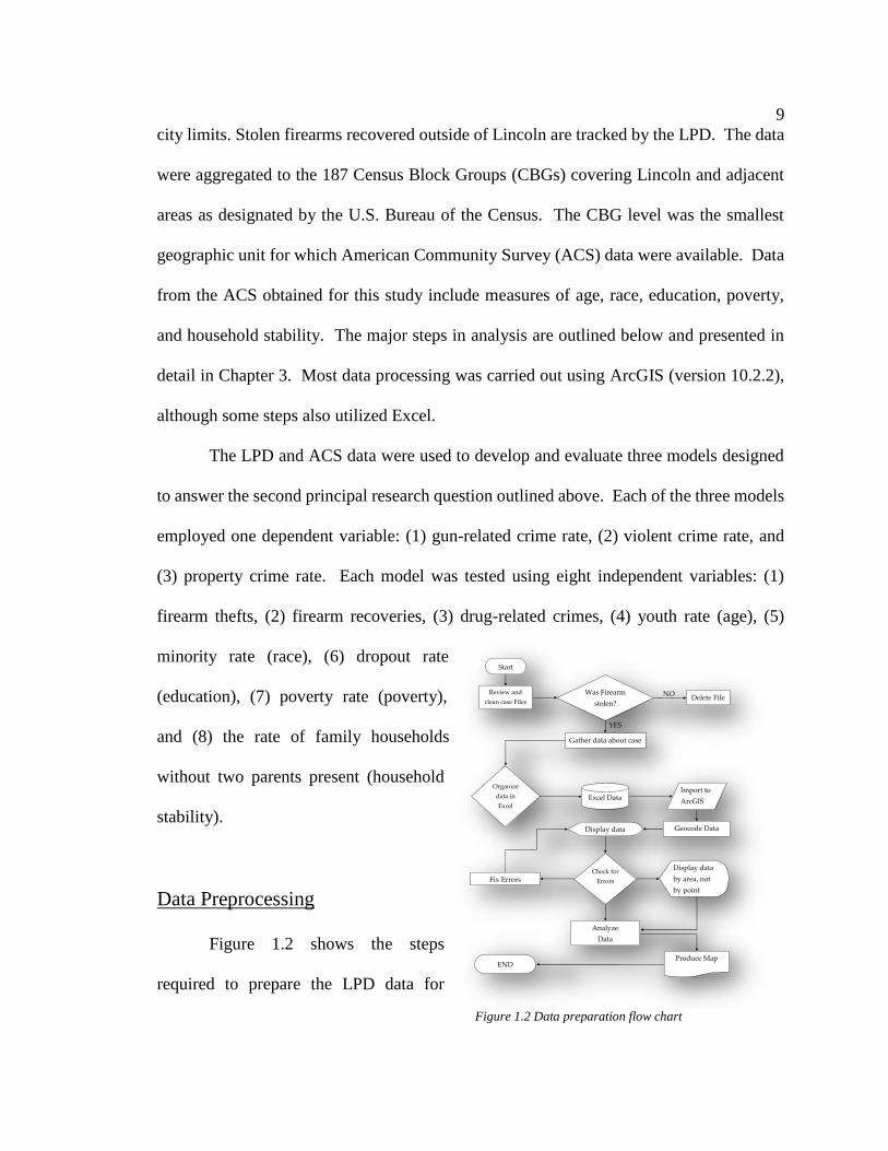
Figure 1.2 shows the steps
required to prepare the LPD data for
NO
YES
Start
Review and
clean case Files
Was Firearm
stolen?
Delete File
Gather data about case
Excel Data Import to
ArcGIS
Geocode Data
Produce Map END
Fix Errors
Analyze
Data
Check for
Errors
Display data
Display data
by area, not
by point
Organize
data in
Excel
Figure 1.2 Data preparation flow chart
10
analysis. All data were assembled and organized using Microsoft Excel. The first step in
data preparation involved cleaning the dataset by removing firearms identified as lost or
listed as a “fake” weapon (e.g. bb gun, pellet, or air soft), as well as items such as display
and carrying cases, ammunition, and accessories (e.g. holster, scope). Each case file was
then reviewed and additional metadata (e.g., owner appraised value of the firearm, the
number of firearms involved in each case, and other descriptive statistics regarding the
incident) were added to each case. The data in Excel were then imported into a GIS
(ArcGIS 10.1) for further analysis. Each point was geocoded using the address given in
LPD reports. Next, the data were used to prepare Tables, charts and choropleth maps.
Statistical Analysis
The methodology utilized for this study is an aggregate of multiple methods as
depicted below (Figure 1.3). First, Hotspot analyses were conducted on the locations of
firearm thefts and recoveries (2010; Grubesic 2006; Levine 2006; Harries 1999; Sherman
1995). Hotspot analyses identify areas where many incidents are clustered. Clustering
suggests that the data are not randomly distributed. Subsequently, choropleth mapping was
used to highlight areas where specific types of crimes occurred. These methods were
employed to address objectives 1, 2, and 3 (i.e. (1) how firearm thefts are spatially
distributed in Lincoln, Nebraska, a typical medium-size U.S. city, (2) where firearms are
recovered in Lincoln, and (3) if the spatial distributions of firearm thefts and recoveries
have changed over the study period 2007-2013).

11
Three models were created for statistical analysis; (1) gun-related crime, (2) violent
crime, and (3) property crime. Each of the three dependent variables underwent a
logarithmic transformation. Correlation matrices were used to determine the strength of
the relationship firearm thefts and recoveries have with the transformed variables.
Stepwise regression was then performed on each model to determine the regression (OLS)
model with the strongest relationship. Results of a Spatial Autocorrelation test revealed
that each of the transformed dependent variables were related to themselves over space.
Subsequently, a robust form of statistics employed Maximum Likelihood Estimation
(MLE) to determine the type of spatial variables missing from the multivariate regression
models.
Map data• Create point and
choropleth maps for each set of data
Hotspot Analysis
• Perform Moran's I analysis on firearm thefts
• Perform Getis Ord Gi* analysis on thefts and recoveries over time
Clustering
• Perform Average Nearest Neighbor Analysis and Spatial autocorrelation to determine if there is clusting in the data and if the varaibles are related to themselves over space
Correlation Matrix
• Create Correlation Matrices for each dependent varaible
Regression
• Perform Multivariate Regression ro each Model developed for this study
Maximum Likelihood Estimation
• Perform Spatial Lag and Error analysis on each model to test for spatial significance
Figure 1.3 Flowchart of methods

12
Implications
It is expected that this study will provide a better understanding of the location of
thefts and recoveries by law enforcement. Although the research will be conducted in
Lincoln, Nebraska, the results should be helpful to many law enforcement agencies
elsewhere to guide them in focusing attention on areas especially prone to firearm thefts.
In addition, this study will demonstrate methods for using geospatial analysis tools to
illuminate firearm theft and recoveries and their contribution to crime.
Research has shown that the incidence of violent crime is correlated with
availability of firearms, especially stolen handguns (Cook and Ludwig 2004; Hoskin
2001; McDowall 1991; Cook 1983). There are, however, different views on how the
research should be interpreted. Some people, including those affiliated with movements
such as the Brady Campaign, believe that improved legislation and increased gun
regulation will reduce the availability of firearms and make violent crimes and theft less
likely (Brady Campaign 2013). Others, including the National Rifle Association (NRA),
believe that easing access to firearms reduces the need to steal and provides individuals
with opportunities to protect themselves in the event someone attempts to use a firearm to
commit a crime on their property or person (National Rifle Association 2013). This
research is expected to increase the understanding of where firearms are being stolen,
where they are recovered and their relation to other crimes. Furthermore, this research is
designed to improve knowledge pertaining to the contribution stolen firearms make to
crime.

13
Thesis Structure
This thesis has been organized into five chapters. Chapter one introduces firearm
violence and the issue of theft, recognizes the deficiencies in other studies and establishes
the need for more research, discusses the research objectives, defines the study area,
defines the data sources, and summarizes the methods used. Chapter two discusses the
current state of violence in the U.S., outlines the importance of stolen firearms, and
examines the distribution methods further and the role of firearm availability affecting
firearm violence. Chapter three further defines the methods in more detail. Chapter four
presents and discusses the results. Finally, in chapter five, the conclusions are examined
and suggestions are made for future research in this area.

14
Chapter 2: Literature Review
Introduction
It is estimated that, in 2011, 467,321 persons were victims of a crime committed
with a firearm in the U.S. (Bureau of Justice Statistics [BJS], 2011). That year, firearms
were used in 68 percent of murders, 41 percent of robberies, and 21 percent of aggravated
assaults across the nation (FBI, 2011). Although these numbers have varied somewhat
over the past 50 years, the high incidence of violent crimes involving firearms have made
firearms a major topic of debate and research.
Improving the understanding of the factors that contribute to gun violence is critical
to law enforcement in order to abate violent crime. Hence, numerous studies have been
conducted to explore the causes of firearms-related violence. Research has shown that
firearms-related crimes are correlated with a wide range of factors that include, but are not
limited to, socio-economic conditions, geographic location, education, exposure to crime,
and availability of firearms (Altheimer 2008, 2010; Altheimer and Boswell 2011; Braga,
Papachristos, and Hureau 2010; BJS 1995, 2001, 2013; Hoskin 2001; Koper 2007;
McDowell 1991). Furthermore, research has shown that criminals rely on numerous
pathways to obtain firearms for criminal activity (Braga et al 2012; Koper 2007; Mayors
Against Illegal Guns 2008, 2010; Sheley and Wright 1993; Wright and Rossi 1986, 1994).
Little research, however, has been conducted on the relationship firearms-related crimes
have with firearm thefts, much less the geography of firearm thefts (Stolzenberg and

15
D’Alessio 2000). To date, no research has been conducted on firearm thefts in Lincoln,
Nebraska.
This chapter provides a selective review of the most relevant literature pertaining
to the prevalence, influences, and contributors of firearms-related crime. Special attention
is given to the role of gun theft. The principal objectives of this chapter are to:
Introduce crime mapping,
Briefly review the current characteristics of firearms-related violence in the
United States,
Summarize what is known about firearm thefts, and
Discuss socio-economic and demographic variables commonly related to
crime.
Mapping Crime
Maps, by definition, show the locations of features, characteristics and/or events
that occur at particular times. For a crime analyst, looking at where and when crimes have
taken place in the past can be very insightful in predicting when and where crimes might
occur in the future. Comparisons of different types of maps (e.g., crimes and socio-
demographic conditions) can also assist in development of hypotheses about factors that
influence crime and suggest means to mitigate criminal activity.
Crime mapping is defined as the process of conducting a spatial analysis of the
distribution of crimes and other issues associated with law enforcement (Boba 2001).
Crime mapping combines the skills of people, the practical use of data and information,

16
and the application of technology to capture, analyze, identify and respond to crime
problems and improve policing performance (Police Standards Unit 2005). The process of
crime mapping takes common map elements like roads, buildings, and natural
characteristics of the physical world like bodies of water and mountains as spatial
references within which crimes occur. Using these geographic variables, combined with
socio-demographic information, the crime analyst attempts to answer the underlying
questions associated with crimes to include, but not limited to, why crime occurs more
frequently in certain areas and what characteristics are associated with high rates of crime.
Today, most crime mapping is accomplished using a Geographic Information
System (GIS). A GIS is software that allows the user to quickly and efficiently capture,
create, store, integrate, manipulate, analyze, and display data related to positions on the
Earth’s surface (Geographic Information Systems 2002). This is done through the use of
multiple layers displaying different sets of data simultaneously (Figure 2.1). The GIS
provides a wide variety of tools for spatial analysis including statistical functions that can
help in understanding patterns, causes and impacts of crime. Widely used GIS software,
such as ArcGIS, is often augmented by
programs such as CrimeStat developed in
1999 as a free add-on which provides
unique graphic and statistical tools for
crime analysts (Levine 2006). A GIS
allows the analyst to create digital
Figure 2.1 GIS layers. Source – Police standards unit 2005

17
documents that can be printed, shared, and manipulated by colleagues.
Toblers’ first law of geography states that “Everything is related to everything else,
but near things are more related than distant things” (Klippel, Hardisty, and Li 2011). Maps
are often used to identify spatial patterns in data to help make decisions and predictions
about the future. Patterns can be classified into four categories: random, uniform,
clustered, or dispersed (Harries 1999). Events that are clustered are usually of special
interest in crime mapping as they indicate where crimes are concentrated, a prerequisite for
addressing criminal activity.
One of the great advantages of using computer technology and GIS to analyze
geographic data is that it facilitates rapid statistical assessment of patterns, trends, and
associations. Clusters, for example, are often verified by using statistical tools such as
Moran’s I (ESRI 2013a). Once clusters of criminal activity (often termed “Hot Spots”) are
identified, maps/data of factors such as population density, demographics, cultural and
social variables can be assessed to determine if and how they may help explain the reasons
crimes occur in certain areas. In addition to using Moran’s I, researchers sometimes use
other methods to define s in crime mapping. Such methods include hierarchical and non-
hierarchical cluster analysis, fuzzy clustering, k-means, and median clustering among
many others (Grubesic 2006). A problem, however, is that different results (i.e., different
conclusions about presence or absence of clustering) may occur when different methods
are used. For these reasons, analysts must practice caution when comparing the results of
different analyses.

18
Maps, of course, can be prepared at a variety of spatial and temporal scales. Crime
analysts and police use maps with different scales to address different types of issues. For
example, the FBI, a federal agency, might be interested in small scale maps portraying
long-term crime trends nationwide, whereas a city police analyst would probably be more
interested in viewing crime trends at a local level (a larger scale) over shorter periods of
time.
The map analyst may also choose to display the data by points showing the
locations of the crimes or aggregate the points to a polygon. In urban mapping, polygons
are often comprised of Census Tracts, police districts, school districts or zip codes
depending on the mapping objective. Some units are subdivided into smaller subunits.
Census Tracts, for example, can be broken into smaller nested Block Groups and again into
Blocks which improve the spatial resolution of the map. Furthermore, the analyst must
choose to express the data in its raw form or as a rate normalized by an additional variable.
For example, the locations of firearm thefts can be aggregated to a CBG and expressed as
a raw total of all firearm thefts committed in the CBG. The raw number could also be
expressed as a normalized rate by dividing the total number of firearm thefts by the total
population or total number of crimes in the CBG. Normalizing the count data allows for
comparison of different values on a common scale. It should be noted that, though smaller
areas such as Census Blocks do provide more precision, obtaining demographic data for a
more robust analysis often becomes more difficult.
In addition to the basic mapping decisions mentioned above, the analyst has a
number of tools in the GIS to perform spatial analyses on the data. These typically include

19
Average Nearest Neighbor (ANN), Getis-Ord General G statistic, spatial autocorrelation
using global Moran’s I, and Ripley’s k-function (ESRI 2013b). Furthermore, the analyst
can choose from several mapping tools to display clusters including, but not limited to:
Cluster and Outlier Analysis using Local Moran’s I and Analysis using Getis-Ord Gi*
(ESRI 2013c). Hot Spot analysis is of particular interest to crime analysts because it shows
areas where events are clustered.
Below are two examples of Hot Spot analyses of vandalism around the city of
Lincoln, Nebraska (Figure 2.2). Areas of high crime (s) are shown in red, areas of low
crimes (Cold Spots) are shown in blue, while neutral areas (Neither Hot nor Cold) are
shown in yellow. Though the two maps are based on the same data, they exhibit differing
patterns. The left image (raw vandalism count) indicates that vandalism is more common
in the downtown area; while the right image (normalized by all crimes) indicates that,
compared to other crimes, vandalism is a bigger issue in the suburbs. While the left image
shows that more vandalism crimes occur downtown, the right images shows that vandalism
accounts for a larger percentage of the total crime rate in the suburbs.
Figure 2.2 Vandalism in the city of Lincoln displayed by raw count data (left) and normalized
with data for all crime incidents (Right). Source – ESRI 2013d

20
Though it is helpful to determine if patterns of criminal activity occur, ultimately
crime analysts need to understand the factors at play in creating such patterns. The theory
of distance decay has often been used to assist in such analyses (Harries 1999). Distance
decay has its roots in Walter Christaller’s central place theory (Lewis Historical Society
2013). Though Christaller has been criticized for his overemphasis of space, the theory
has been a strong model for almost a century and has greatly affected crime analysis.
Basically, distance decay states that people are more likely to carry less and make many
trips when traversing small distance; as distance traversed increases, however, they are less
likely to make as many trips and will likely be willing to transport larger loads for each
trip. Most crime analysts believe that as distance decreases, the motivation to commit a
crime also decreases.
Crime analysts also make use of the theory of “Routine Activities Theory” also
known as RAT (Cohen and Felson, 1979; Sutton 2010). In general, analysts suggest that
there are three major components to crime: a likely offender, a suitable target, and the
presence or absence of a “guardian” capable of discouraging, stopping or preventing the
crime (e.g., a person, a security system or even a wall). Criminals are thought to wait for
“safe opportunities” to commit crimes. Potential criminal activity is reduced, for instance,
as population density increases it become more likely that a bystander will observe and
report criminal activity. Paradoxically, it has long been known that criminal activity is
more common in urban areas than rural areas because of the increased numbers of potential
targets and criminals. In theory, the frequency of crime should be lower in urban areas

21
because of the increase amount of potential guardianship. To account for such
observations, analysts must consider the contributing factors to crimes.
Maps, it must be remembered, are ultimately simply tools. They usually do not, in
and of themselves, directly answer specific questions about the incidence, causes or
prevention of crime. It is the job of the analyst to find the relationships between the factors
being displayed and criminal behavior (e.g., relationships to social and physical factors).
The analyst develops a hypothesis, tests and evaluates the hypothesis with the aid of GIS
and other tools, accepts or rejects the original hypothesis, and then reevaluates as
necessary.
Lincoln, Nebraska has utilized GIS for spatial analyses for nearly two decades. In
1999, Tom Casady, the former Chief of Police and current Director of Public Safety,
implemented CrimeView, a GIS application developed by the Omega Group, Inc. (ESRI
2003). The application is still widely used today by the entire police department.
Advantages of this application allow police officers and analysts to process large amounts
of data visually in a short period of time. Proactive Police Patrol Information (P3i) is
another application being used by the police in Lincoln (Lincoln Police Department 2011).
This is a new location based application introduced by Tom Casady and the University of
Nebraska-Lincoln in 2011 that employs location based services relaying crime data for
police officers in the field. Though the police in Lincoln are very familiar with spatial
applications, no research has been conducted on the theft of firearms in Lincoln. In this
thesis, GIS and spatial statistics will be used to help achieve a better understanding of how

22
firearm thefts, firearm recoveries, and crimes are spatially distributed within the
community of Lincoln, NE with assistance from the LPD.
Firearms-Related Violence in the United States
Geography of Firearm Violence
Previous research has shown that firearms violence is often tied to location (BJS
2013, and 1995). Regionally, the South tends to have the highest rates of firearms-related
violence while the Northeast maintains the lowest average rates (Figures 2.3 and 2.4).
Again, it is noteworthy that firearms violence was observed to have dropped from its
highest point in 1993 before stabilizing around the turn of the century.
When considering geography at a local
level, urban areas always show the highest
incidence of firearms-related violence and rural
areas generally the lowest (Figure 2.5). Cities
with a population between 250,000 and half a
Figure 2.3 Firearm homicides by region from
1993 to 2010. Source – BJS 2013 Figure 2.4 Nonfatal firearm violence by region from
1997 to 2011. Source – BJS 2013
Figure 2.5 Nonfatal firearm violence by urban-
rural location from 1994 to 2011. Source – BJS
2013

23
million exhibited the largest amount of violence in 1997 whereas cities with a population
between half a million and 1 million were highest in 2001. Some studies of firearms-
related violence have been conducted at even finer scales (Braga et al 2010). They found
the firearm-related violence in Boston was concentrated in a select number of street
segments and intersections, which they referred to as micro places. They suggested that
the large amount of violence in urban areas could be explained by a select number of these
micro places.
The BJS (2013) found that the largest percentages (over half) of both fatal and
nonfatal violence occurs in or near a victim’s home. These results suggest that crime is
closely related to residential areas in urban settings. The research also suggests that certain
residential areas may be considered micro places or s for crime. Furthermore, less than ten
percent of violent crimes occur in commercial areas. Also, a considerable amount of
firearm violence takes place in parking lots and other open outdoor areas.
Data on Firearm-related Violence
There is no single national registry that contains information about every crime
committed in the U.S.; however, there are a multitude of sources that are commonly used
to assess crime at the national level. The BJS, for example, has used official police records
and surveys of both criminals and victims to create data to make reasonable deductions
about how often firearms were used in crimes, what categories of firearms are being used
in crimes, the type of firearm being used, and the users of firearms in crimes.

24
In 2011 the BJS submitted its most recent report on firearm violence in the U.S.
(BJS 2013). This report aggregated data from a number of sources including; the National
Crime Victimization Survey (NCVS), the National Center for Health Statistics (NCHS)
CDC Web-Based Injury Statistics Query and Reporting System (WISQARS), the School-
Associated Violent Death Surveillance Study (SAVD), the National Electronic Injury
Surveillance System All Injury Program (NEISS-AIP), the FBI’s Uniform Crime Report
(UCR), Supplemental Homicide Reports (SHR), the Survey of Inmates in State
Correctional Facilities (SISCF), and the Survey on Inmates in Federal Correctional
Facilities (SIFCF).
The BJS (2013) reported that, from a peak of 18,243 reported homicides in 1993,
the number of homicides in the U.S. fell dramatically to 10,828 in 1998 before stabilizing
(Figure 2.6). In 2011 there were some 11,101 reported homicides. In 1993 there were
approximately 1.5 million nonfatal victims of firearms-related violence in the U.S. (Figure
2.7). That number has fallen over the period from 1993-2011. The 2011 count was
467,300.
Figure 2.6 Firearm homicide from 1993 to 2011.
Source – BJS 2013 Figure 2.7 Nonfatal firearm victimization from 1993
to 2011. Source – BJS 2013

25
As a raw percentage, firearm use in 1994 accounting for 9.3 percent of all violent
crimes (BJS 2013; Table 2.1). However, homicides as a subset of all firearm violence
reached an all-time high in 2008 accounting for 3.2 percent of all firearm violence. These
numbers suggest that though criminals are resorting to firearm use less often, they still
heavily rely on firearms.
Table 2.1 Criminal Firearm Violence from 1993 to 2011. Source – BJS 2013

26
Though the rate of firearm use has
changed over time, the choice of firearm and
type of crime involving a firearm has not
changed much at all (Tables 2.2 and 2.3). A
large percentage of homicides involve a
firearm with aggravated assault a very
distant second, and robbery third. For both
fatal and nonfatal violence, handguns are
used significantly more often than rifles or
shotguns (combined) throughout the time period of 1993 to 2011 (Table 2.2). This is
reflected both in the raw number and the percentages.
Survey data collected from state and Federal inmates has shown that criminals
prefer all forms of handguns to long guns because of their light weight and concealable
nature (BJS 2001; Sheley and Wright 1993; Wright and Rossi 1986, 1994). Furthermore,
handguns are also generally less expensive and are produced in larger quantities. In a 1997
Table 2.2 Criminal firearm violence, by type of firearm from 1994 to 2011.
Source – BJS 2013
Table 2.3 Percent of violence involving a
firearm by type for crime from 1993 to
2011. Source – BJS 2013

27
survey of prison inmates, over 80 percent of state and federal inmates who were carrying
a firearm at the time of offense were in possession of a handgun (BJS 2001). Furthermore,
in a 2000 ATF report on youth offenders, 9 of the top 10most traced firearms were in fact
handguns (ATF 2000a).
In 2001, the BJS reported criminals who used firearms to commit crimes were
predominantly non-white (Figures 2.8 and 2.9). Furthermore, it was reported that victims
of violent crime were usually non-white (BJS 2001). Statistics from the 2013 BJS report
are supported by data collected by other researchers (Sheley and Wright 1993; Wright and
Rossi 1986, 1994). The BJS found that during the 1993 to 1999 period there was a dramatic
drop in firearm use within the black community, a drop that was much greater than all other
groups combined. Though there was a small drop in the white community the Hispanic
community actually saw a rise in use during this period.
It is noteworthy that this trend is not reflected in firearm use in nonfatal firearm
offenses as all races saw a dramatic drop during the 1993 to 1999 period. It should be
noted that use during nonfatal events is expressed as a rate per 1,000 and is much greater
than use for homicide which is expressed as a rate per 100,000. Considering this fact, all
fluctuations in Figure 2.9 are much greater than Figure 2.8.
Figure 2.8 Fatal firearm violence by race1993 – 2010.
Source – BJS 2013 Figure 2.9 Nonfatal firearm violence by race and
Hispanic origin from 1994 to 2011. Source – BJS 2013

28
Age also played a very large role in firearm use as over 60 percent of state inmates
and 40 percent of federal inmates were under the age of 24. These findings are also
supported by other data (Sheley and Wright 1993; Wright and Rossi 1986, 1994). The BJS
(2013) found that in 1993 and 1994 the largest percentage use of firearms in both fatal and
nonfatal offenses was by persons between 18 and 24 years of age Table 2.4). Since 1994
these numbers have been cut in half for homicides and almost quartered in nonfatal
offenses.
Firearms Theft
Theft of firearms is a great concern for law enforcement and the general public
because stolen firearms are often used to commit crimes. Individuals who steal firearms
commit crimes with those firearms, trade stolen firearms with other criminals, and add to
the unregulated secondary market. Criminals resort to stealing firearms because of
convenience, necessity, insufficient funds to purchase, inability to involve a third party in
a straw purchase, to obtain more than one firearm in an area where acquiring several
firearms is prohibited and/or suspicious, and selling stolen firearms is very profitable. This
Table 2.4 Fatal and nonfatal firearm violence by age from 1993 to 2011.
Source – BJS 2013

29
section provides a synopsis of key literature on the dimensions of gun theft and the use of
stolen weapons in crime.
A number of previous studies have focused on where and how criminals obtain
firearms (e.g., Kleck 1999, 2009; Wright and Rossi 1986, 1991). Kleck (1999) notes that
stolen firearms are a major source of guns used in crime. Wright and Rossi (1986, 1991)
found that 32 percent of prison inmates they interviewed in a survey personally acquired
their most recent handgun from theft. In the same study, 46 percent were certain the firearm
was stolen, while an additional 24 percent thought the firearm they used in a crime was
stolen. Thus, up to 70 percent of the firearms used in crimes by the prison population
surveyed may have been stolen.
In 2012, NCIC reported a total of 190,342 lost or stolen firearms across the nation
(ATF 2013). However, this very likely underestimates the incidence of thefts. Kleck
(1999), for example, estimates that, on average, there are at least 750,000 firearms stolen
every year. Kleck (2009) attributed such discrepancies to two factors: (1) respondents who
are prohibited from owning a firearm will most likely not report the theft or loss of their
firearm, and (2) 2.2 firearms per theft is most likely low considering that the average gun
owner owns 4-5 firearms (Cook, et al 1995). One point of agreement, however, is that
residential burglaries are consistently the major source of stolen firearms (Kleck 2009).
Age
Research has shown that juveniles (17 and under) and youths (18 to 24) are more
likely to be involved in the theft, possession, use, and trade of stolen firearms (BJS 1995;

30
Wright and Rossi 1986, 1994). This stems from several reasons. First and foremost,
juveniles are proscribed from purchasing and possessing firearms themselves. Youths
under the age of 21 are only allowed to purchase long guns, which as discussed earlier, are
less desirable due to their size and difficulty to conceal. Second, stealing a firearm requires
absolutely no investment of funds and therefor is free to the thief. Juveniles and youths
also acquire stolen firearms through unregulated purchases on the secondary market. Many
stolen firearms are sold on the secondary market because they cannot be sold to FFLs, are
untraceable, and easily transferred. Purchasing stolen firearms on the secondary market
also tend to be less expensive because of the profitability and no financial investment on
the thief’s behalf.
Geography of Firearms Theft
The geography of firearm violence and theft show similar patterns. One study that
examined the relationship between legal and illegal firearm availability found that stolen
guns are highly correlated with violent crime at the county level in South Carolina
(Stolzenberg and D’Alessio 2000). The same study found that rural areas maintained lower
rates of violent crime and firearm theft than more densely populated areas. Furthermore,
in the U.S., urban and suburban areas have higher rates of firearm thefts as well as firearms-
related crime (BJS 2012). The South was the region that sustained the highest rate of
firearm theft while the Northeast sustained the lowest rate. As discussed earlier, the South
was also the region that maintained the highest rate of firearms-related violence in the U.S.
Though these numbers may seem an indicator that more firearms mean more violence

31
because the South maintains the highest rates of firearm ownership, this assumption would
not be entirely true. This hypothesis would only maintain validity if the South sustained a
rate of theft in general similar to the rest of the country. This is not the case. The South
maintained the highest rate of burglary and property crimes while the North maintained the
lowest rates. The rate of firearms-related violence is simply a reflection of the rate of theft
which is, of course, in turn related to the prevalence of firearms in homes. If firearms are
not available in a burglarized home, the thief cannot take a gun. Existing research has
sparked the interest of researchers to start examining the correlations and effect firearm
thefts have on violent crimes. Much research, however, has only examined smaller scale
areas and even less research has examined small or mid-sized cities specifically. This issue
will be addressed in this study by examining firearms theft in Lincoln, Nebraska.
Firearm Theft Data Issues
The ATF is the federal agency that is charged with monitoring firearms in the U.S.
and is regarded as the number one source of data collected at the national level. However,
the ATF is not capable of collecting complete and comprehensive data. Problems include
(1) voluntary reporting by law enforcement, (2) the public not reporting the stolen or
missing firearms, or (3) the inability to identify recovered firearms due to serial numbers
being obliterated (ATF 2013). Furthermore, the ATF data are based on NCIC data that
typically is not screened for duplicates and, as noted above, not all law enforcement
participate regularly in using this federal database. Hence, ATF data should not be

32
considered complete, although most researchers acknowledge that they should be regarded
as the most accurate data available.
Though reporting by law enforcement is not at 100 percent, it is very high. The
major inaccuracies with the data come from the public not reporting thefts and obliterated
serial numbers. The public may not report the thefts because they are proscribed from
possessing the firearm in the first place, are unaware the firearm has been stolen, do not
know the serial number, do not care the firearm has been stolen, or most commonly, the
owner is related to the thief, and the owner will attempt to recover the firearm without
involving the police. Quite often the owner of the firearm will report the firearm missing
without knowing a friend or family member was involved in the theft. Upon realizing that
the weapon was taken by someone they are close to, the charges are often dropped and the
firearm is not classified as stolen. Many weapons that are stolen can be classified by some
as a borrowed weapon, and not stolen. It should also be noted that due to the widespread
ownership of firearms, in many cases, stealing a firearm is most likely to occur in a home
instead of a business as mentioned above. For example a thief is more likely to steal a
firearm from someone they know because they are more than likely to get away with the
crime due to the existing relationship with the victim provided the victim discovers there
firearm is missing. Additionally, the thief is aware of the presence of the firearm, and in
many cases can obtain the firearm without much difficulty as opposed to the difficulty of
stealing from an arms dealer or pawn shop.
The other issue is serial number obliteration. Criminals often destroy the serial
number on their firearms to prevent the firearm from being traced by the ATF. The ATF

33
regards obliterated serial numbers as a key indicator that the firearm was illegally traded
on the secondary market (Braga et al 2002). Even though possession of a firearm with an
obliterated serial number is a crime, many still do so to prohibit tracing the origins of the
firearm. 1n 1999 11 cities were involved in the Youth Crime Gun Interdiction Initiative
(YCGII). Possession of obliterated serial numbers in these 11 cities was highest among
youths who were already proscribed from possessing a firearm (ATF 2000a, 2000b; Braga
et al 2002). Nearly 20 percent of firearms recovered from youths had an obliterated serial
number (Kennedy, Piehl, and Braga 1996; Braga et al 2002).
There is no current way to discern the exact number of firearm thefts occurring each
year nationwide, however there is evidence that firearm thefts do contribute to a larger
portion of violent crimes. Though ATF data is unavailable for Lincoln, the LPD does
maintain a detailed comprehensive database of all crimes, including firearm thefts. For
this research, the LPD database will be used to compare firearm thefts and violent crimes
in Lincoln as previous research has done in other places and at the national level.
Demographics
Research has shown that firearms-related crimes are correlated with a wide range
of factors that include, but are not limited to, socio-economic conditions, age, race,
education, geographic location, household status, and exposure to crime (Altheimer 2008,
2010; Altheimer and Boswell 2011; Braga, et al 2010; BJS 1995, 2001, 2013; Hoskin 2001;
Koper 2007; McDowell 1991). This section will discuss several of these factors and their
relevance to this thesis.

34
Age: Results from the ATF Youth Crime Gun Interdiction Initiative (YCGII) showed
youths (18 to 24) accounted for 33.3 percent of crime, the largest of any 7-year age group
(U.S. Department of Justice, Bureau of Alcohol, Tobacco, Firearms and Explosives (ATF)
2000a). Furthermore, more crime guns are recovered from the youth 7-year age grouping
than any other 7-year age grouping, juvenile or adult. Research has shown a strong
relationship between stolen firearms and the use of illicit firearms by youth (Cook and
Ludwig 2004; Braga and Kennedy 2001). Finally, youths have the highest rate of
recovered firearms with obliterated serial numbers, which are good indicators that a firearm
has been stolen (ATF 2000). For these reasons, the cohort of youth is the age group of
most interest for this study.
Education: Several previous studies have used a measure of education as a variable for
comparing crime rates (Altheimer 2008; Lochner and Moretti 2001; Sheley and Wright
1993; Stolzenberg and D’Alessio 2000). Altheimer (2008) found that areas of more
education were subject to lower rates of assault. Lochner and Moretti (2001) found that
the rate of incarceration for adults dramatically decreases for those who obtain a high
school degree or equivalent. Sheley and Wright (1993) found in their survey of inmates
that the modal education attainment level was 10th grade. Finally, some research has used
dropout rates as control variables (Stolzenberg and D’Alessio 2000).
Wealth: Socio-economic variables have been used in many previous studies (Altheimer
2008; Altheimer and Boswell 2011; Hoskin 2006). Altheimer (2008) found that an

35
increase in levels of poverty lead to an increase in the odds of an individual falling victim
to a robbery involving a firearm. Furthermore, Altheimer and Boswell (2011) found that
levels of poverty greatly impact homicide rates. Anthony Hoskin (2006) found that a
measure of poverty, the number of people on welfare programs, was highly correlated with
the homicide rate in a multi-national study.
Race: An abundance of research has been conducted on the relationships between minority
populations and crime (BJS 2013; Cohen and Tita 1999; Rosenfeld 1999). The BJS report
shows that crime between 1993 and 2011 was especially high in the African American and
Latino communities (2013). Cohen and Tita (1999) found a significant relationship
between homicide rates and Census Tracts that had an African American population of at
least 25 percent in Pittsburg, Pa. Rosenfeld, working in St. Louis, Mo, found that an
overwhelming number of participants in both gang and non-gang homicides were African
American (1999).
Home Stability: Several studies have examined the relationship of home stability with
crime (Altheimer 2010; Sampson 1986, and 1987; Sun, Triplett, and Gainey 2004).
Altheimer (2010) used the divorce rate as a measure of family disruption. Results from the
analysis showed that family disruption was negatively correlated with assault in general,
yet had a strong positive correlation with assaults involving a firearm. Sampson (1986 and
1987) found that family disruption was significantly related to neighborhood crime, both
violent and non-violent. Sun, Triplett, and Gainey (2004) found that the effects of family
36
disruption had the strongest relationship with assaults. For these reasons, single parent or
divorced households should be considered as a possible demographic variable for studying
crime.
Summary and Conclusion
This chapter discussed several key topics that pertain to crime mapping, firearms-
related violence, firearm theft statistics, and measures of demographics related to crime.
Previous research has shown that both firearm-related violence and gun theft are typically
carried out by young adults (18-24) and predominantly affects non-white races. More
densely populated areas and the southern states are most afflicted with firearms-related
violence.
Means by which law enforcement and citizens can work to abate gun theft and gun
violence are not as clear. Some believe that firearm thefts are insignificant and that the
majority of measures taken to reduce violence should target arms dealers and legislation
regulating ownership. Other research has shown that firearm thefts contribute a significant
amount to firearms-related violence and most certainly warrant more attention. It should
be noted, however, that accurate measures of the rate of firearm thefts is very difficult
because of two major variables; failure to report the theft and obliterated serial numbers.
With the advent of the GIS, crime analysis has been greatly advanced. In this thesis
a GIS-based methodology was employed to achieve the four principle objectives of this
research (1) how firearm thefts are spatially distributed in Lincoln, Nebraska, a typical
medium-size U.S. city, (2) where firearms are recovered in Lincoln, (3) if the spatial
37
distributions of firearm thefts and recoveries have changed over the study period 2007-
2013, and (4) whether the spatial distributions of firearm thefts and/or recoveries are related
to spatial patterns of other crimes and/or socio-demographic characteristics (e.g., income,
age or ethnicity) of Lincoln’s populace. The next chapter will discuss the data collected
and the methods used in this study. The subsequent chapter will discuss the results from
the methods employed in this thesis. Finally, the last chapter in this thesis will analyze the
importance of the results and make recommendations on future research needs.

38
Chapter 3: Methods
Introduction
This chapter explains the methods employed to achieve the objectives posed in
chapter 1. The overall methodology is depicted in Figure 1.3. Data used in this research
were derived from a unique database on crimes developed by the Lincoln, Nebraska Police
Department (LPD), a geodatabase of population characteristics developed by the U.S.
Bureau of the Census American Community survey (ACS) and, data collected about thefts
and recoveries of firearms by the author. All statistical data for thefts and recoveries were
initially organized in Microsoft Excel and later imported into the ArcGIS 10.2.2 software
from the Environmental Systems Research Institute (ESRI). Geospatial data obtained from
the LPD and the Census in the form of shapefiles or geodatabases were directly imported
into ArcGIS. Statistical analyses used ArcGIS, Microsoft Excel, and the Geoda software
developed by Luc Anselin at Arizona State University (ASU) (ASU 2014). This chapter
is organized into five sections: (1) study area, (2) data collection, (3) geodatabase
development, (4) data analysis, (5) and conclusion.
Study Area
This research focuses on Lincoln, Nebraska (Figure 3.1), a community estimated
to have a 2010 population of approximately 258,000 (Table 3.1). Although the population
of Lincoln is somewhat younger and less racially and ethnically diverse than the nation as
a whole, Lincoln is, nevertheless, generally representative of many mid-size cities in the

39
central U.S. (Table 3.2). As the state capital of Nebraska and home of the University of
Nebraska-Lincoln, government and education serve as key pillars of the local economy;
however, the economy is quite diverse overall, bolstered by commercial, agribusiness,
insurance, and health care (City-Data 2009).
Race Demographics
RACE Lincoln Percent USA Percent
Total population 258,379 100 308,745,538 100
One Race 250,717 97 299,736,465 97.1
White 222,331 86 223,553,265 72.4
Black or African American 9,824 3.8 38,929,319 12.6
Hispanic or Latino 16,182 6.3 50,477,594 16.3
American Indian and Alaska Native 2,073 0.8 2,932,248 0.9
Asian 9,773 3.8 14,674,252 4.8
Native Hawaiian and Other Pacific Islander 147 0.1 540,013 0.2
Some Other Race 6,569 2.5 19,107,368 6.2
Two or More Races 7,662 3 9,009,073 2.9
Race alone or in combination with one or more other races
White 229,200 88.7 231,040,398 74.8
Black or African American 13,653 5.3 42,020,743 13.6
American Indian and Alaska Native 4,061 1.6 5,220,579 1.7
Asian 11,483 4.4 17,320,856 5.6
Native Hawaiian and Other Pacific Islander 386 0.1 1,225,195 0.4
Some Other Race 7,890 3.1 21,748,084 7
Table 3.1 Racial Demographics of Lincoln. Source – U.S. Census Bureau 2013
Figure 3.1 Study Area for research on Firearm Thefts and Recoveries in Lincoln,
Nebraska. Source – U.S. Census Bureau and Lincoln Police Department
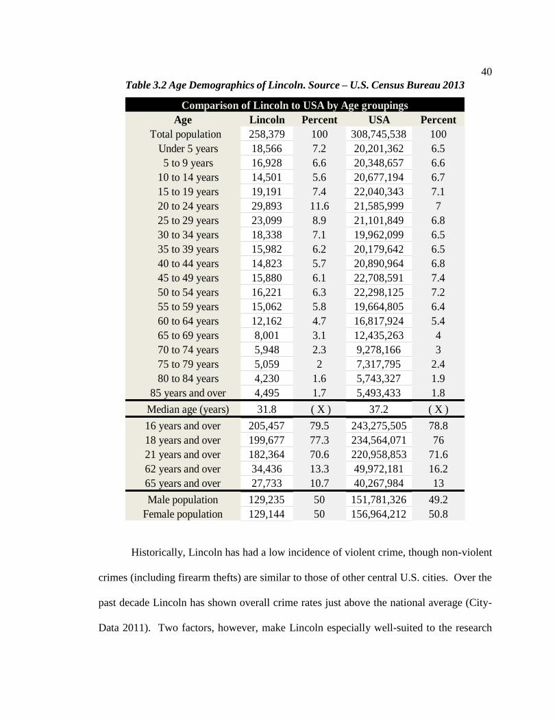
40
Historically, Lincoln has had a low incidence of violent crime, though non-violent
crimes (including firearm thefts) are similar to those of other central U.S. cities. Over the
past decade Lincoln has shown overall crime rates just above the national average (City-
Data 2011). Two factors, however, make Lincoln especially well-suited to the research
Age Lincoln Percent USA Percent
Total population 258,379 100 308,745,538 100
Under 5 years 18,566 7.2 20,201,362 6.5
5 to 9 years 16,928 6.6 20,348,657 6.6
10 to 14 years 14,501 5.6 20,677,194 6.7
15 to 19 years 19,191 7.4 22,040,343 7.1
20 to 24 years 29,893 11.6 21,585,999 7
25 to 29 years 23,099 8.9 21,101,849 6.8
30 to 34 years 18,338 7.1 19,962,099 6.5
35 to 39 years 15,982 6.2 20,179,642 6.5
40 to 44 years 14,823 5.7 20,890,964 6.8
45 to 49 years 15,880 6.1 22,708,591 7.4
50 to 54 years 16,221 6.3 22,298,125 7.2
55 to 59 years 15,062 5.8 19,664,805 6.4
60 to 64 years 12,162 4.7 16,817,924 5.4
65 to 69 years 8,001 3.1 12,435,263 4
70 to 74 years 5,948 2.3 9,278,166 3
75 to 79 years 5,059 2 7,317,795 2.4
80 to 84 years 4,230 1.6 5,743,327 1.9
85 years and over 4,495 1.7 5,493,433 1.8
Median age (years) 31.8 ( X ) 37.2 ( X )
16 years and over 205,457 79.5 243,275,505 78.8
18 years and over 199,677 77.3 234,564,071 76
21 years and over 182,364 70.6 220,958,853 71.6
62 years and over 34,436 13.3 49,972,181 16.2
65 years and over 27,733 10.7 40,267,984 13
Male population 129,235 50 151,781,326 49.2
Female population 129,144 50 156,964,212 50.8
Comparison of Lincoln to USA by Age groupings
Table 3.2 Age Demographics of Lincoln. Source – U.S. Census Bureau 2013

41
proposed here. First, Lincoln has a long history of using digital geospatial data and GIS in
law enforcement (Casady 2013; ESRI 2013d). As a consequence numerous datasets are
available to support research on firearms theft and crime. In addition, the research has
greatly benefited from the personal interest, experience and collaboration provided by Mr.
Tom Casady, a leader in the use of GIS in law enforcement and currently public safety
director for Lincoln (formally, the Sheriff of Lancaster county and the Chief of Police in
Lincoln) (Casady 2013). For this research, he has provided the author access to unique
data unavailable to the general public.
Database Development
Lincoln Police Department
The primary data used in this study were obtained from the LPD. The data cover
the period from January 1st 2007 to December 31st 2013 and include the locations of (1) all
reported thefts of firearms (stolen firearms dataset), (2) all firearms recovered by the LPD
in Lincoln regardless of whether they were stolen or not (recovered firearms dataset), (3)
all crimes (all crimes dataset), and (4) gun-related crimes (gun-related crimes dataset).
Two datasets were created from the stolen firearms and recovered firearms datasets and
include the locations of (1) all reported thefts of firearms that were subsequently recovered
(stolen recovered dataset), and (2) all firearms recovered by the LPD that were originally
stolen (recovered stolen dataset). An additional three datasets were created from the all
crimes dataset and include the locations of (1) violent crimes committed in Lincoln (violent
crimes dataset), (2) property crimes committed in Lincoln (property crimes dataset), and

42
(3) drug-related crimes committed in Lincoln (drug-related crimes dataset). These datasets
are shown in the Table 3.3. It should be noted that, while the data for stolen firearms are
available only for sites within the city limits, the data for recoveries of firearms stolen in
Lincoln is geographically unrestricted. In many cases, criminals commit crimes within the
city and subsequently travel outside the city limits. Stolen firearms recovered outside of
Lincoln are tracked by the LPD through the NCIC.
Table 3.3 List of datasets obtained and created from Lincoln Police Department
Dataset Description
Stolen firearms All firearms stolen in Lincoln Nebraska
Stolen recovered All firearms stolen in Lincoln that were recovered
Recovered firearms All firearms recovered in Lincoln regardless of theft
Recovered stolen All firearms recovered in Lincoln that were originally stolen
All crimes All crimes committed in Lincoln
Gun-related All crimes involving a firearm in Lincoln
Violent crimes All homicides, assaults, robberies, and rapes in Lincoln
Property crimes All thefts and vandalisms in Lincoln
Drug-related crimes All crimes involving drugs of any type in Lincoln
The stolen firearms dataset enumerates all firearms reported to the LPD as lost or
stolen. The firearms recovered dataset summarizes all weapons recovered for any reason
by the LPD. The methods used to gather the data for both datasets are shown in Figure
3.2. These datasets are complete listings of all thefts and recoveries associated with the
LPD between 2007 and 2013. In situations where the firearm was not reported stolen, there
is no report and the firearm is not listed in the data.

43
Because of the advanced digital reporting system implemented by the LPD, there
is a substantial amount of detail in their reports. All data for thefts and recoveries are
reported and added to each case file immediately after being submitted by the reporting
officer. All firearm thefts reported to the LPD have a case number and at least a general
description of the location of the theft. The detail of each report depends on the reporting
officer. In many cases there was no address or location that could have been used to
identify the place and/or time of theft (e.g., auto theft or mugging in a public area). In these
cases the reporting officer gave as detailed a description as possible based on the closest
known street address while including a time frame the theft may have occurred in. The
recovery location was only provided by the LPD if the firearm was recovered by the LPD
•Cases, gun bags, holsters, ammunition, scopes, (BB, air soft , and pellet guns)Remove False Reports
•Handgun, shotgun, rifleClassify Gun Type
•Use the address listed in the reports for stolen address and recovered addressFind Location
•Narative data for thefts and reoveries, status of case, relative information
Gather Data Case by Case
•Fix discrepancies in data by consulting with Tom CasadyQuality Control
•Import data into ArcMap using an address locatorGeocode
Figure 3.2 Methods used to gather data about firearm thefts and recoveries in Lincoln

44
or if the firearm was related to an ongoing investigation that involved the LPD at the time
of recovery. For firearms not recovered by the LPD, data from the NCIC was used (FBI
2008). Any time a stolen firearm has a serial number reported by the victim of the crime
it is listed with the FBI as missing property. Upon recovery there has to be a request for
the removal of the firearm from the NCIC by the recovering police department. These
requests can be tracked and therefore can be used to determine the place the weapon
traveled to before the recovering police department obtained the firearm. Once again, an
exact location may not be reported by the recovering law enforcement agency (e.g., a
highway stop on an interstate). This data reveal the last known location and the final
destination before recovery, however it is impossible to tell where the firearm traveled in
between these locations. Basic descriptive data on the actual theft include type of theft,
value of the firearm, firearm specifications, property descriptive data, and data about
persons involved (Table 3.4).
Other data available from the LPD include names, ages, and residence of the
victims, persons reporting, suspects (if any), and persons responsible (if any). This
information is only accessible to individuals with security clearance and, though accessible
to the author, was not collected or reported on in this study (other than the exact location
of the theft or recovery) to protect the identities of those involved. The LPD provides
additional data listed in Table 3.5 and 3.6. As mentioned above, the third and fourth
datasets, stolen firearms recovered and firearms recovered stolen were created from the
data gathered from the initial two datasets and therefore will have the same data fields.

45
Table 3.4 Addition descriptive data provided by LPD reports
Burglary Forced entry
Larceny From building or automobile
Robbery Violent crime theft
Embezzelment Very infrequent
Value Appraised by owner
Serial number Only when available to owner
Make and model Brand and type of firearm
Caliber or gauge The type of ammunition required
Type of firearm Handgun, rifle, or shotgun
Damage Any damage to the property casued during theft
Value of damage The cost of repairs required to fix damage
Locked If the firearm was secured by the property and or within the property
Location The closest known address where the firearm was recovered
Time The date and time of day when the firearm was recovered
Age of PR Age of the person firearm was recovered from
Theft Categorization
Firearm descriptive
Property Reports
Recovery
Table 3.5 Data collected on the recoveries of firearms
Hyp_Path URL without the case number
Hyperlink URL with case number
Prop_RPT Property report for gun
INC_Num Incident number
Description Description of firearm recovered
Type Type of gun
Make Brand of gun
Date_RCVRD Date the firearm was recovered if recovered
RCVRD_Address Address where the firearm was recovered
Drug Did the theft or recovery of the firearm involve drugs of any sort
Gang Did the theft or recovery of the firearm involve a gang of any sort
Violence Was the firearm involved with or related to a violent crime?
TOV Type of violence (Assault, Robbery, ect…)
PR_Age Age or person responsible at recovery
COR Circumstances of recovery
Serial Serial number of firearm
Stolen Was the firearm stolen
Crime Was the firearm recovered related to a crime?
RKY Case number
Recovered Dataset

46
Table 3.6 Data collected on the thefts of firearms
Prop_RPT Property report for gun
RKY Case number
Hyp_Path URL without the case number
Hyperlink URL with case number
Call_Type Reason given for police involvement
Date RPRTD Date theft was reported to the police
Description Description of firearm stolen
Make Brand of gun
Serial Serial number of firearm if reported
Date_RCVRD Date the firearm was recovered if recovered
Status Status of the case
Type Type of Gun
Stolen_Addres Address or closest possible address to the location where the theft occur
Stolen_State Nebraska
Stolen_County Lancaster
Stolen_Local Lincoln
EPDT Earliest possible date of theft
Value Owner appraised value of firearm stolen
Theft_Type Type of theft (Residential, business, ect..)
TNGS Total number of guns stolen
Premise_Lock If the building/room was locked
Gun_Locked If measures were taken to secure the firearm separately that locking the premises
Target Was the gun the target of the theft or an opportunity theft
Drug Did the theft or recovery of the firearm involve drugs of any sort
Gang Did the theft or recovery of the firearm involve a gang of any sort
RCVRD_Address Address where the firearm was recovered if recovered
RCVRD_State State firearm was recovered in
RCVRD_County County of recovery
RCVRD_Local Local of recovery
PR_Age_Theft Age of person responsible for theft
PR_Age_RCVRD Age of person responsible at recovery
COR Circumstances of recovery
TOR Type of recovery (How the firearm was recovered)
TTRSEPT Time to recovery since earliest possible theft
TTRSTR Time to recovery since theft reported
CLOG Current location of gun
TDOG Terminal destination of gun
ORTT Owner relation to thief
RON Recovered or not recovered
ACI Case report that signifies where the information was found
See_Case Other related case with more information
ACI Case report that signifies where the information was found
See_Case Other related case with more information
Stolen Dataset

47
The all crimes dataset is a shapefile of all crimes covered by the LPD between
January 1st 2007 and December 31st 2013. This shapefile does not include all calls for
service which would have included false crime reports such as suicides, threats, and other
non-criminal related incidents. The sixth dataset, all gun-related crimes, is a shapefile of
all crime that involved a firearm. This dataset includes all crimes where a firearm was
present and not necessarily used in the commission of the crime. The seventh dataset,
violent crimes, is an aggregate shapefile of all homicide, assault, robbery, and rape cases.
This shapefile was created by selecting the four attributes just described and creating a new
layer from the all crimes shapefile. The eighth dataset, property crimes, is an aggregate
shapefile of all unlawful takings or destructions of property. This shapefile was created by
selecting all attributes related to the theft or destruction of property and creating a new
layer from the all crimes shapefile. Though quite often there is overlap, particularly with
property crimes, these locations represent the exact locations of the crime, not the home
addresses of persons involved or the location the report was made from. Finally, the ninth
dataset, drug crimes, is a shapefile of all crimes where drugs were present at the time of
arrest or involved drugs at a later time. This shapefile was created by selecting all
possession, distribution, and narcotics crimes from the all crimes shapefile.
American Community Survey (ACS) Data
Demographic data used in this study came from the U.S. Bureau of the Census.
Data from the 2010 Census and the 2012 American Community Survey (ACS) are used at
the Census Block Group (CBG) level. The data obtained were measures of age, race,

48
education, wealth, and a home stability which were used to explain the relationship violent
crimes, gun-related crimes, and property crimes have with social, economic, and
demographic characteristics of Lincoln residents (Table 3.7). Data estimated from the ACS
were organized in columns by CBG. Each column was organized with a unique ACS
lookup ID. In order to create the appropriate data, ACS lookup IDs were used to aggregate
the data appropriately and are displayed here as a reference.
Table 3.7 Aggregated variables collected from the American Community Survey
ACS Variables Measure Description
Age Youth All males 18 to 24
Race Minority All non-Caucasian persons
Education Dropout Persons 25 and over without a high school degree or
equivalent
Wealth Poverty Households living under the poverty level
Home Stability Broken Homes Family households with one parent present
Age: As noted in Chapter 2, most gun-related crime is perpetuated by youths 18-24 years
old. Since the vast majority of crimes committed with a firearm are carried out by males,
females were excluded. This variable was aggregated in its raw form by combining the
count data by CBG for males age 18 and 19, 20, 21, and 22 to 24 years old. These data
were summed and divided by the total male population of each CBG (Table 3.8).
Table 3.8 ACS variables used to measure the Youth rate by CBG
Variable ACS Lookup ID
Total male population age 18 to 19 B01001e7
Total male population age 20 B01001e8
Total male population age 21 B01001e9
Total male population age 22 to 24 B01001e10
Total male population B01001e2
Youth = (B01001e7 + e8 + e9 +e10) / e2
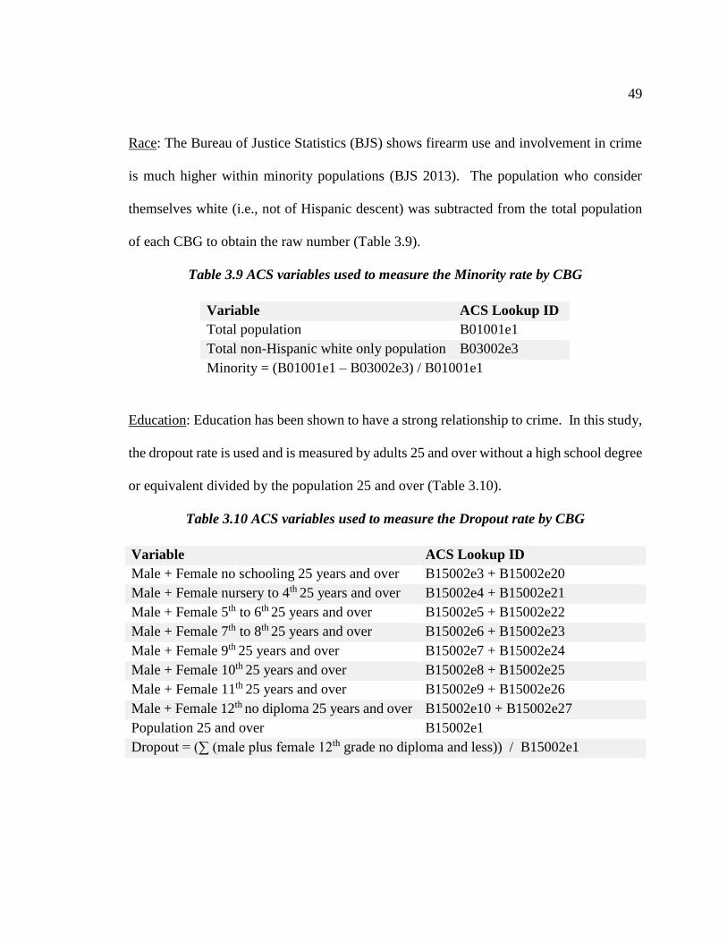
49
Race: The Bureau of Justice Statistics (BJS) shows firearm use and involvement in crime
is much higher within minority populations (BJS 2013). The population who consider
themselves white (i.e., not of Hispanic descent) was subtracted from the total population
of each CBG to obtain the raw number (Table 3.9).
Table 3.9 ACS variables used to measure the Minority rate by CBG
Education: Education has been shown to have a strong relationship to crime. In this study,
the dropout rate is used and is measured by adults 25 and over without a high school degree
or equivalent divided by the population 25 and over (Table 3.10).
Table 3.10 ACS variables used to measure the Dropout rate by CBG
Variable ACS Lookup ID
Male + Female no schooling 25 years and over B15002e3 + B15002e20
Male + Female nursery to 4th 25 years and over B15002e4 + B15002e21
Male + Female 5th to 6th 25 years and over B15002e5 + B15002e22
Male + Female 7th to 8th 25 years and over B15002e6 + B15002e23
Male + Female 9th 25 years and over B15002e7 + B15002e24
Male + Female 10th 25 years and over B15002e8 + B15002e25
Male + Female 11th 25 years and over B15002e9 + B15002e26
Male + Female 12th no diploma 25 years and over
B15002e10 + B15002e27
Population 25 and over B15002e1
Dropout = (∑ (male plus female 12th grade no diploma and less)) / B15002e1
Variable ACS Lookup ID
Total population B01001e1
Total non-Hispanic white only population B03002e3
Minority = (B01001e1 – B03002e3) / B01001e1

50
Wealth: Previous research has shown that the relationship socio-economic status has with
crime (Althiemer 2008). There are many ways to measure the economic status of an
individual or family: total income, unemployment, entitlement program recipient, and
many more. For the purpose of this study the rate of households living under the poverty
level was chosen as a measure of economic inequality and a possible explanatory variable
for the regression analysis. This is a measure of income required to meet the minimum
needs of a family defined by the government. The rate is dependent on the number of
individuals present in the household and therefore income requirements change as the
family size increases. The variables chosen for this study are individuals and families
below the poverty level (Table 3.11).
Table 3.11 ACS variables used to measure the Poverty rate by CBG
Home Stability: Previous studies have used household stability as a measure for comparing
crime rates (Altheimer 2010). For this study, home instability was defined as the absence
of one or more parents. This measure was used as a possible explanatory variable for the
regression analysis (Table 3.12).
Table 3.12 ACS variables used to measure the Broken Homes by CBG
Variable ACS Lookup ID
Total number of households B17017e1
Household income in the past 12 months below poverty level B17017e2
Poverty = B17017e2 / B17017e1
Variable ACS Lookup ID
Family household, male householder, no wife present
B11001e5
Family household, female householder, no husband present B11001e6

51
Geodatabase Development
All data to be used in ArcGIS were converted to geodatabases (Figure 3.3).
Initially, the data for firearm thefts and recoveries were collected and aggregated using
Microsoft Excel 2013; however, files were automatically saved as .xlsx, a format not
recognized by the latest versions of ArcGIS. Thus the Excel sheets first had to be saved as
.xls files so they would be acceptable by the ArcGIS software.
Point shapefiles were created of both the stolen and recovered firearm data sets
using the World Geocode Service provided by ArcGIS Online (ArcGIS 2013) in ArcMap.
Over 90 percent of addresses in both datasets were geocoded without any issues. Files that
exhibited problems were manually geocoded. The additional two datasets for stolen
Total family households B11001e2
Broken Home = (B11001e5 + B11001e6) / B11001e2
• Organize unprojected dataCreate file Geodatabase for shapefiles
• Thefts in Lincoln
• Recoveries in LincolnGeocode using World Geocode
Service (ArcGIS Online)
• Block Group shapefile and geodatabase
• States
• Counties
Download and extract Census data for Lincoln
• All crimes from January 1st 2007 to December 31st 2013
• All crimes with a gun from January 1st 2007 to December 31st 2013Obtaine data from LPD
• Violent Crimes
• Property Crimes
• Drug Crimes
Create data from LPD
• Lincoln (LPD)
• World street map and Lincoln Basemap (ESRI)Obtain base maps
• Create new field in each data set
• set each row equal to 1
• add points to bg polygon by performing a join by location
Joined 9 data sets by location to Block Group Shapefile
• ACS data was joined to the TIGER shapefile after fields were caluclated in the TIGER geodatabase shaptfile
Join ACS data
• Census data multiplied by 100,000 (data is already expressed as a proportion)
• LPD- Divide by population of block group and multiply by 100,000Convert counts to rates
• One for Albers projection
• One for Nebraska State Plane projectionCreate additional Geodatabases
Figure 3.3 Geodatabase development steps
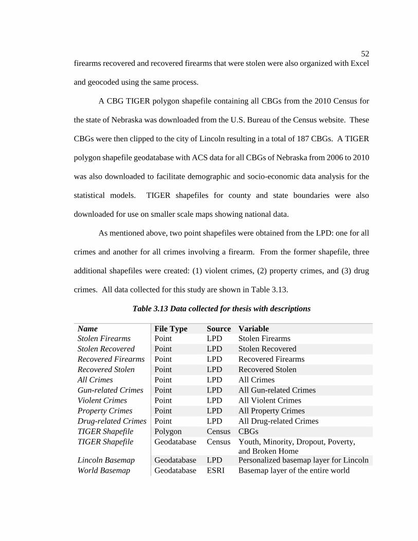
52
firearms recovered and recovered firearms that were stolen were also organized with Excel
and geocoded using the same process.
A CBG TIGER polygon shapefile containing all CBGs from the 2010 Census for
the state of Nebraska was downloaded from the U.S. Bureau of the Census website. These
CBGs were then clipped to the city of Lincoln resulting in a total of 187 CBGs. A TIGER
polygon shapefile geodatabase with ACS data for all CBGs of Nebraska from 2006 to 2010
was also downloaded to facilitate demographic and socio-economic data analysis for the
statistical models. TIGER shapefiles for county and state boundaries were also
downloaded for use on smaller scale maps showing national data.
As mentioned above, two point shapefiles were obtained from the LPD: one for all
crimes and another for all crimes involving a firearm. From the former shapefile, three
additional shapefiles were created: (1) violent crimes, (2) property crimes, and (3) drug
crimes. All data collected for this study are shown in Table 3.13.
Table 3.13 Data collected for thesis with descriptions
Name File Type Source Variable
Stolen Firearms Point LPD Stolen Firearms
Stolen Recovered Point LPD Stolen Recovered
Recovered Firearms Point LPD Recovered Firearms
Recovered Stolen Point LPD Recovered Stolen
All Crimes Point LPD All Crimes
Gun-related Crimes Point LPD All Gun-related Crimes
Violent Crimes Point LPD All Violent Crimes
Property Crimes Point LPD All Property Crimes
Drug-related Crimes Point LPD All Drug-related Crimes
TIGER Shapefile Polygon Census CBGs
TIGER Shapefile Geodatabase Census Youth, Minority, Dropout, Poverty,
and Broken Home Lincoln Basemap Geodatabase LPD Personalized basemap layer for Lincoln
World Basemap Geodatabase ESRI Basemap layer of the entire world

53
Basemaps for displaying the data at the local and national scale were also obtained.
A basemap of Lincoln was obtained from the LPD and saved as an additional geodatabase.
A World basemap was also downloaded from ESRI online for displaying data at the
national scale (ArcGIS 2013).
All 9 point shapefiles were joined to the TIGER CBG polygon shapefile. This was
executed by first, adding a new numeric column to each point shapefile and naming it
Count. Using the ArcGIS field calculator, each cell in that column was then set to equal 1.
A join was then performed by joining data from each point shapefile to the polygon
shapefile by selecting the “Join data from another layer based on spatial location”.
The 5 demographic variables in the ACS geodatabase (Youth, Minority, Dropout,
Poverty, and Broken Home) were joined to the TIGER shapefile by using the ObjectID as
the lookup value. Subsequently, all raw count data (e.g., firearm thefts, recoveries, and
crimes) were normalized by dividing each variable by the total population of each CBG
and then multiplying by 100,000. The Census data were already expressed as a proportion
of the population, and, thus were simply multiplied by 100,000.
All data at this point were only displayed with Geographic Coordinate System,
North American Datum 1983 (GCS NAD 1983). An additional two geodatabases were
created for conducting spatial analyses at differing scales. For local data in Lincoln, a
geodatabase was created. All data were copied and then projected using the Nebraska State
Plane System (NAD 1983) projection. For display purposes, however, a custom
Transverse Mercator projection tailored to the city of Lincoln was used to reduce visual

54
distortion. For the entire U.S., a national geodatabase was created. All data were projected
using U.S. Contiguous Albers Equal Area Conic projection
Data analysis
Several different analytic methods were used to address the principal objectives of
this research: to determine (1) how firearm thefts are spatially distributed in Lincoln,
Nebraska, a typical medium-size U.S. city, (2) where firearms are recovered in Lincoln,
(3) if the spatial distributions of firearm thefts and recoveries have changed over the study
period 2007-2013, and (4) whether the spatial distributions of firearm thefts and/or
recoveries are related to spatial patterns of other crimes and/or socio-demographic
characteristics (e.g., income, age or ethnicity) of Lincoln’s populace.
Objectives 1 and 2:
In order to describe the state of firearm thefts and recoveries in Lincoln, several
Tables, Figures, and maps had to be generated using the data collected. A combination of
Microsoft Excel and Word along with ArcGIS were used to calculate the values within the
Tables, Figures, and maps. Three topics were addressed when processing the data: (1) the
distribution of firearm thefts in Lincoln, (2) the distribution of firearm recoveries in
Lincoln, and (3) the distribution of gang involvement in firearm recoveries.
Maps were created using basic point and choropleth mapping techniques. Eight
maps were generated in this process, two for each dataset, one point and one choropleth:
(1) firearms thefts (from the stolen firearms dataset), (2) firearm thefts recovered (from the

55
stolen recovered dataset), (3) firearm recoveries (from the recovered firearms dataset), and
(4) firearms recoveries that were stolen (from the recovered stolen dataset).
Two spatial statistical analyses were subsequently conducted on the eight datasets
generated above. First, the Average Nearest Neighbor (ANN) tool in ArcGIS was used to
determine whether or not each of the four point distributions were clustered or randomly
dispersed. Spatial patterns are considered clustered when the z-score (a measure of
standard deviations from the mean) results from the ANN test are less than -2.58 (or more
than 2.58 standard deviations below the mean). Second, the Spatial Autocorrelation
(Global Moran’s I) tool in ArcGIS was used to determine in if the four polygon
distributions were related to themselves over space, which is indicative of clustering. A
Queen contiguity matrix and row standardization were used. With the matrix, each
polygon looks to all other polygons it shares a border or corner with. Areas that are
considered neighbors are assigned a value of 1 while non-neighbors are assigned a value
of 0. Furthermore, the matrix allows for row standardization which reduces the amount of
sampling bias possible with spatial distributions. A pattern in this case is considered
spatially auto correlated, and therefore clustered, when the z-score is equal to or greater
than 2.58.
Subsequent Hot Spot analyses were conducted utilizing the data that had been
aggregated to the CBG TIGER shapefile. Three maps were created utilizing the “Cluster
and Outlier Analysis tool” also known as Local Moran’s I. Each map depicts firearm thefts
normalized by a different variable: (1) property crimes, (2) all crimes, and (3) population.
Results show areas of clustering and by type of clustering (1) High-High, (2) High-Low,

56
(3) Low-High, (4) Low-Low, and (5) Not Significant. Take for example firearm thefts
normalized by property crimes. High-High signifies a large number of thefts in an area
with many property crimes while Low-Low signifies a small number of firearm thefts in
an area that does not have many property crimes. The High-Low and Low-High signify
outliers. For this analysis, a Contiguity Edges and Corner spatial weight matrix was
utilized. This weight matrix suggests that CBGs are affected by neighboring CBGs.
The final map generated for objective 2 displays the entire contiguous United
States. The map show the direct Euclidian distance for firearms stolen in Lincoln to their
final destination before being recovered by law enforcement. This was accomplished
through a number of steps. First, using the management “Join Field” function, the X and
Y coordinates for the theft and recovery locations were joined from the stolen firearms
dataset to the stolen recovered dataset using the address where the firearm was stolen to tie
the two datasets together. Second, the “XY To Line” function was used to draw the lines
between the locations of theft and recovery. The resulting map displays the direct path
between the point of theft and the point of recovery. The distance was calculate in meters
and converted to miles. The data for distances were then used in the Tables generated for
Objective 2.
Objective 3:
The third objective of this study addresses the changing spatial distributions of
firearms stolen and recovered between 2007 and 2013 in Lincoln. In order to perform this
analysis, the data were organized by year. In order to add perspective to the analysis, the

57
distributions for all crimes, violent crimes, and property crimes were also analyzed. A new
layer containing all five datasets for each year was created. Since the time span covers
seven years and there are five variables being analyzed, a total of 35 new fields were
created within a new shapefile. Each layer was then appended to the new TIGER polygon
shapefile. This was done in the same fashion as before by creating a new field, setting it
equal to 1, and joining it to the polygon shapefile by location. This process produced
several null values, particularly for the stolen and recovered datasets when no points were
located within a polygon. For data quality purposes, all null values were converted to 0.
The “Hot Spot analysis (Getis-Ord Gi*)” tool was then used to create 35 new layers for
each of the fields generated in the previous step. At the end of the process there were five
maps for each of the seven years, each displaying Hot and Cold spots.
Objective 4:
Objective four addressed the possible relationship between firearm thefts and
recoveries with other crimes. First, it was first necessary to define the dependent and
explanatory variables of interest. Three statistical models were developed, each testing a
different dependent variable: (1) violent crime, (2) gun-related crime, and (3) property
crime. The data for all three variables were skewed; thus, a logarithmic transformation
was used to make the distribution of each variable more normal. Because the dependent
and independent variables were aggregated to the CBG level and expressed both as raw
count data and as rates, both versions of each variable were examined for a more normal

58
distribution. Data were compared as histograms and visually interpreted (Figures: 3.4, 3.5,
3.6, 3.7, 3.8, and 3.9).
Figure 3.4 Frequency Distribution for the rate of Gun-Related Crimes in Lincoln (Left) and the logarithmic
transformation of the rate of Gun-Related Crimes in Lincoln (Right).
Figure 3.5 Frequency Distribution for the raw count total of Gun-Related Crimes in Lincoln (Left) and the logarithmic
transformation of the raw count total of Gun-Related Crimes in Lincoln (Right).

59
Figure 3.6 Frequency Distribution for the rate of Violent Crimes in Lincoln (Left) and the logarithmic transformation of
the rate of Violent Crimes in Lincoln (Right). Figure 3.7 Frequency Distribution for the raw count total of Violent Crimes in Lincoln (Left) and the logarithmic
transformation of the raw count total of Violent Crimes in Lincoln (Right).
Figure 3.8 Frequency Distribution for the rate of Property Crimes in Lincoln (Left) and the logarithmic transformation
of the rate of Property Crimes in Lincoln (Right).

60
After the visual analysis was conducted, the most normal distribution of the two
possible for each variable was chosen. For example, the logarithmic transformation of the
rate of gun-related crimes was more normal than the logarithmic transformation of the raw
count data for gun-related crimes. Similarly, the logarithmic transformations of the raw
count data for violent crimes and property crimes were more normal than the
transformation of the rate of violent crimes and property crimes. For the gun-related
dependent variable, the rates of the independent variables were used. For the violent crimes
and property crimes dependent variables, the raw count independent variables were used.
Next, the relationship of firearm thefts and recoveries with each dependent variable
was examined. The strength of each relationship was analyzed using the Pearson’s
product-moment correlation coefficient (Equation 3.1).
Equation 3.1 Pearson’s product-moment correlation coefficient
𝒓 = ∑ (𝑿𝒊 − �̅�)(𝒀𝒊 − �̅�)𝒏
𝒊=𝟏
√∑ (𝑿𝒊 − �̅�)𝟐𝒏𝒊=𝟏 √∑ (𝒀𝒊 − �̅�)𝟐𝒏
𝒊=𝟏
= ∑ (𝑿𝒀)𝒏
𝒊=𝟏
√∑ (𝑿)𝟐𝒏𝒊=𝟏 √∑ (𝑿)𝟐𝒏
𝒊=𝟏
where
∑ is the summation symbol
𝐗 = 𝐗𝐢 − 𝐗
𝐗𝐢 = the observed value for 𝐗
Figure 3.9 Frequency Distribution for the raw count total of Property Crimes in Lincoln (Left) and the logarithmic
transformation of the raw count total of Property Crimes in Lincoln (Right).

61
𝐗 = the mean 𝐗 value
𝐘 = 𝐘𝐢 − 𝐘
𝐘𝐢 = the observed value for 𝐘
𝐘 = the mean 𝐘 value
This was accomplished by generating a correlation matrix in Microsoft Excel and
then evaluating the resulting coefficients with a t-test. Correlation coefficients (r) range
from -1 to 1. The strongest linear relationships are -1 and 1 while the weakest liner
relationship is 0. A positive correlation signifies that as one variable increases, the other
variable tends to increase as well. A negative correlation signifies that as one variable
increases, the other tends to decreases. Peter Rogerson suggests that values closer to 0 can
be significant provided the sample size is large (Rogerson 2010). The minimum absolute
value of r needed to achieve significance where α = 0.05 and the sample size of n > 30 can
be determined by the equation 2/√𝑛 (Rogerson 2010). Since there are 187 CBGs being
used in this analysis, this number served as the sample size. The minimum r value is
therefore .146 because 2
√187= .14625448. The null hypothesis that 𝒓 = 𝟎 for each
correlation coefficient was then tested using the t-test (Equation 3.2). A t-Table reveals
that the critical values of t, using α = 0.05 in a two-tailed test with 185 degrees of freedom,
are ±1.9729. For t-statistics with a value of less than -1.9729 or more than +1.9729, the
null hypothesis can be rejected.
Equation 3.2 t-test for Correlation Coefficient
𝒕 =𝒓√𝒏 − 𝟐
√𝟏 − 𝒓𝟐
where
𝒓 = the correlation coefficient
𝒏 = the sample size

62
The correlation matrix determines if there is a correlation between firearm thefts
and recoveries, but does not attempt to explain the dependent variable using thefts or
recoveries. The second test performed was a multivariate regression analysis which
attempted to explain the variance in the dependent variable (Equation 3.3).
Equation 3.3 Ordinary Least Squared Multiple Regression
For this statistical analysis, the objective was to see if a combination of two or more
independent variables could explain a significant amount of the variance of each dependent
variable. There are several key social and economic characteristics of populations that
seem to be highly correlated with crime (see Chapter 2). For this analysis, in addition to
the independent variables from the previous statistical analyses (firearm thefts and
recoveries), the five demographic variables from the ACS and the drug-related crime
variable mentioned above were incorporated as well. A total of eight possible explanatory
variables were used in the multivariate regression analysis.
𝒀𝒊 = 𝜷𝟎 + 𝜷𝟏𝑿𝟏𝒊 + 𝜷𝟐𝑿𝟐𝒊+. . . +𝜺𝒊 where
𝒀𝒊 = Dependent variable, what is being predicted or explained
𝜷𝟎 = the constant or intercept
𝜷𝟏 = the slope for 𝑿𝟏𝒊
𝑿𝟏𝒊 = the first independent variable that is explaining the variance in 𝒀𝒊
𝜷𝟐 = the slope for 𝑿𝟐𝒊
𝑿𝟐𝒊 = the second independent variable that is explaining the variance in 𝒀𝒊
𝜺𝒊 = the error term, captures all other factors that influence 𝒀𝒊 other than 𝜷𝒋𝑿𝒊𝒋
j = independent variable, 1,….,n i = observation, 1,….,n

63
Because it was assumed that the locations of the variables are spatially
autocorrelated, the dependent variables were tested for spatial autocorrelation in.
Subsequently, a spatially weighted matrix was created using the “Generate a Spatial
Weights Matrix” tool in ArcGIS. The spatial weights matrix was created specifically for
Lincoln CBG polygon set and employs a Queen contiguity spatial relationship.
Next, the “Exploratory Regression” tool in ArcGIS was utilized. Each model was
generated separately for a total of three different analyses, each using the spatial weights
matrix developed in the previous step. A maximum of five and a minimum or two
explanatory variables were specified to limit the total possible number of variables in the
equation while requiring at least two or more variables to be used in the analysis. A Table
for multivariate correlation coefficients revealed that for 150 degrees of freedom with five
variables requires a correlation coefficient (R) of at least .290 for a 95 percent confidence
interval (Arkin and Colton 1964). With this taken into consideration, a minimum
coefficient of determination (𝑅2) for the model to be significant was set at .0841. Only
results that exceeded this number were presented. The cutoff p-value was set as 0.05 which
means that only results with at least a 95% confidence level were reported. Furthermore,
multicollinearity can occur when several explanatory values are being compared. The
variance inflation factor (VIF) was designed to account for this issue. Rogerson suggests
that, as a common rule of thumb, a VIF greater than 5 indicates potential multicollinearity
issues (Rogerson 2010). Therefore, a value of 5 was set as the maximum value for the VIF.
The Jarque Bera p-value tests the model’s residuals for a skewed distribution
suggesting biased results. This tool also tests the residuals for spatial autocorrelation. The

64
null hypothesis for Jarque Bera states that the residuals of the equation have a normal
distribution. A significant p-value rejects the null hypothesis and indicates that the
residuals are, in fact, non-normal. When the residuals are non-normal, the coefficients (β-
estimates) are likely biased. For this reason, a p-value cutoff of .1 was chosen. Only values
with a p-value of 0.1 or greater were reported. The null hypothesis for the spatial
autocorrelation test is that the residuals are not spatially autocorrelated. Smaller values
reject the null hypothesis and indicate that the model is flawed because the residuals are
spatially auto correlated, and therefore, the results may be misleading. If residuals are
spatially auto correlated, there is most likely a key explanatory variable missing from the
regression equation (most likely the spatial autocorrelation of the original values in the
equation which is not accounted for in classic regression models). A significant p-value
was set at 0.1. Only values of .1 or greater were reported. Residuals that are spatially
autocorrelated will most likely also return a significant Jarque Bera p-value resulting in the
failure of that test as well.
Because each of the dependent variables were spatially autocorrelated none of the
results in each of the three models passed any of the criteria. Therefore, each model was
run a second time without any specifications for these variables to determine the strongest
relationship for each variable. The resulting highest 𝑅2 in addition to the least amount of
additive explanatory variables was choosen as the best fit for each model. Each model was
then tested using Spatial Error (Equation 3.4) and Spatial Lag (Equation 3.5) Maximum
Likelihood Estimation (MLE) methods in Geoda. Results from this test account for spatial
autocorrelation as an explanatory variable. The log likelihood was used to compare the

65
Lag and Error models to the classic Ordinary Least Squared (OLS) model. A higher value
suggests that space is a key explanatory variable for the equation, therefore, a more
significant model.
Equation 3.4 Spatially Lagged term which is substituted for the error term (𝜺𝒊) in the
Multiple Regression equation
Equation 3.5 Spatial Error term which is substituted for the error term (𝜺𝒊) in the
Multiple Regression equation
Summary and Conclusion
The methodology used in this study involved several key steps; (1) data collection,
(2) geodatabase development, and (3) data analysis. Data collection involved gathering
data from police case files and organizing the information in a Microsoft Excel spread
sheet. These data were then geocoded using the ArcGIS software. Three geodatabases
were created, each containing geocoded datasets, downloaded datasets, and datasets
generated from the previous datasets.
𝜺𝒊 = 𝝆𝑾𝒊𝒀𝒊 + 𝝐𝒊 where
𝝆 = the spatial autoregressive parameter
𝑾𝒊 = the spatial weights matrix
𝒀𝒊 = the Dependent variable
𝑾𝒊𝒀𝒊 = the spatially lagged dependent variable
𝝐𝒊 = the independent error term
If 𝒀𝒊 does not depend on neighboring 𝒀𝒊 values, 𝝆 = 0
𝜺𝒊 = 𝝀𝑾𝜺𝝃 + 𝝐𝒊 where
𝝀 = the spatial autoregressive coefficient for error lag 𝑾𝜺
𝑾𝜺 = the spatial weights matrix of lagged error terms
𝝃 = the Vector of uncorrelated error terms
𝝐𝒊 = the independent error term
If there is no spatial correlation between error terms, then 𝝀 = 0

66
Data analysis involved generating Tables, graphs, Figures, and maps from several
software packages, Microsoft Excel and Word, ArcGIS, and Geoda. A cluster analysis was
conducted on the thefts and recoveries of firearms using the Moran’s I method. Statistical
analyses were conducted in Excel, ArcGIS, and Geoda. First a correlation matrix was
developed in Microsoft Excel. A t-test was performed on the resulting significant values.
Subsequently, Regression analysis was conducted in ArcGIS and then tested for Spatial
Lag and error models in Geoda. Finally, a Hot Spot analysis was conducted on five
variables over seven years using the Getis-Ord Gi* method. Results from these analyses
are presented and discussed in Chapter Four.

67
Chapter 4: Results
Introduction
This chapter presents the results of the analysis described in Chapter 3. Results are
presented, discussed, and interpreted in the context of the research objectives. Several
maps, Tables, and Figures were generated for the discussion on the spatial distributions of
firearm thefts and recoveries outlined in objectives 1 through 3. Finally, this chapter
concludes with a discussion of the key findings revealed by this research.
Objectives 1 and 2
Spatial Analysis of Firearm Thefts in Lincoln, Nebraska
In order to identify areas of spatial clustering and discuss the spatial distributions
of firearm thefts several maps were created. For objective 1, a total of three Tables, seven
maps, and one Figure were generated for analysis (Tables 4.1, 4.2, and 4.3; Figures 4.1,
4.2, 4.3, 4.4, 4.5, 4.6, 4.7, and 4.8). An analysis of the maps was conducted and will be
discussed here. Between January 1st 2007 and December 31st 2013 there were a total of
733 firearms stolen and reported to the LPD (Table 4.1). On average, just under two
firearms were stolen per theft which is similar to the 2.2 Figure presented by Kleck (2009)
in the literature review. Furthermore, just over half of the firearms stolen were the sole
target of the theft; nothing else was taken. Finally, just under one-third of firearms stolen
and reported to the LPD were recovered with over three-fourths of the recovered firearms
being recovered in Lincoln.

68
Firearm thefts are shown in two ways, by point data and by CBGs (Figures 4.1 and
4.2). Figure 4.1 shows the actual locations of firearm theft incidents and does not account
for the number of firearms stolen per theft. A visual analysis reveals that firearm thefts
occurred across the entire city of Lincoln. Conversely, Figure 4.2 shows the total number
of firearms stolen by CBGs and is reflective of the actual total number of firearms stolen.
This map reveals a very different pattern than Figure 4.1 displays. This map suggests that
firearm theft is a bigger issue in the peripheral parts of the city. One CBG of particular
interest is located in the southern central part of the city. Unlike the surrounding CBGs,
theft is relatively high. This in part is because of a theft that occurred in 2007 at Scheels
All Sports, a large sporting department store in Lincoln, where 79 firearms were stolen in
a single incident. Though this type of incident is rare and Lincoln has never seen a theft of
comparable magnitude, this CBG should not be considered an outlier due to the remaining
18 firearms stolen over the same time period. Figure 4.3 shows the same data by CBD
only expressed as a rate instead of raw count data.
Table 4.1 General descriptive data for firearm thefts between 2007 and 2013
Measure Value
Firearms stolen 733
Firearm thefts 374
Average # of firearms stolen per theft 1.96
Average value of stolen firearm $368
Thefts where firearm was the target 385
Total stolen firearms recovered 237 (32.3%)
Recovered in Lincoln 181 (76.4%)
Recovered outside of Lincoln 56 (23.6%)

69
Figure 4.2 Firearm Thefts in Lincoln, Nebraska, 2007 – 2013
Figure 4.1 Firearm Thefts in Lincoln, Nebraska by CBG, 2007 – 2013

70
Subsequent Hot Spot analyses revealed significant areas of clustering for firearm
thefts in Lincoln. Figure 4.4 shows the level of significant clustering of firearm thefts
compared to property crimes along the eastern edge of the city limits (High-High
clustering). This map suggests that firearm thefts are high in the eastern part of the city
and in a small area southeast of the central business district (CBD) because of higher
property crimes. Furthermore, the CBG shown in orange is where Scheels is located and
probably reflect the high number of firearm thefts in an area that generally has fewer
property crimes (High-Low clustering). Adjacent to the orange CBG shown in white is a
residential area that has a relatively low number of firearm thefts and a large number of
property crimes (Low-High clustering). The black and orange CBG most likely reflect the
fact that there were only a few incidents of theft where a large number of firearms were
Figure 4.3 Rates of Firearm Thefts in Lincoln, Nebraska by CBG, 2007 – 2013

71
taken. The black CBGs should be more susceptible to firearm thefts because of the higher
number of property crimes. The orange and white CBGs however, are most certainly
unusual. The analyses did not reveal any CBGs with Low-Low clustering.
Figure 4.5 shows a very similar pattern (Figure 4.4). Unlike Figure 4.4, however,
Figure 4.5 displays the relationship between firearm thefts and all crimes, including, but
not limited to property crimes. Once again, the eastern edge of the city is shown as a
significant area of High-High clustering where firearm thefts and all crimes are higher than
expected. Furthermore, the CBG where Scheels is located is once again shown in orange
suggesting that the high number of firearm thefts are occurring in an area that generally
has lower levels of crimes. The higher prevalence of white CBGs around the orange CBG
suggests that all crime is more prevalent in those areas while firearm thefts are generally
lower.
Finally, Figure 4.6 displays areas of firearm theft and population clustering. Unlike
the previous two maps, the eastern edge of the city is not an area of High-High clustering
because of the change to a lower population density. The CBGs classified as High-High
clustering are just east of the CBD in an area where the residential population is relatively
dense compared to the periphery of the city. Additionally, the same pattern of High-Low
and Low-High clustering shown in orange and white in Figure 4.5 is present in Figure 4.6.
Though these maps suggest some interesting trends, the results presented here must
be interpreted with caution. A Queen contiguity weight matrix was employed in this
clustering analysis and must be accounted for. A CBG is considered an outlier when, by
comparison, an adjoining CBG exhibits a very dissimilar pattern. For example, the orange

72
CBG where Scheels is located had 97 firearm thefts over the time period data was collected
for this study. This number is most certainly an outlier being affected by the 79 firearms
stolen from Scheels. In the data collected for this study, the no other theft comes close to
the amount of firearms stolen from Scheels, not does any CBG have nearly as many thefts
as the CBG Scheels is within. Conversely, the adjoining areas shown in white are
considered Low-High areas of clustering because the number of thefts is relatively low
when compared to the orange CBG. With that said, the results should not be considered
bias, they simply display the type of relationship between the adjoining CBGs.
Figure 4.4 Cluster Analysis of Thefts Normalized by Property Crimes in Lincoln, Nebraska, 2007 – 2013

73

74
Figure 4.5 Cluster Analysis of Thefts Normalized by all Crimes in Lincoln, Nebraska, 2007 – 2013
Figure 4.6 Cluster Analysis of Thefts Normalized by Population in Lincoln, Nebraska, 2007 – 2013

75
Firearm thefts by type of theft are summarized in Table 4.2 and shown in Figure
4.7 below. It is apparent that residential thefts are the single greatest source of firearm
thefts. The majority of the remaining firearm thefts were from businesses and automobiles.
It should be noted that, in this study, when a firearm was removed from a car, the theft was
considered auto even though in many cases the automobile was located in a residential area
and sometimes in a driveway. Figure 4.7 suggests several patterns. First, firearm thefts
occur across the entire city. Both residential and auto thefts have no obvious spatial pattern.
Conversely, thefts from businesses and storage facilities suggest linear patterns around
major transportation routes. There are a number of possible explanations for these patterns,
however, the most reasonable explanation is that firearm thefts simply follow a similar
pattern to land use.
Figure 4.7 Firearm Thefts in Lincoln, Nebraska by Type of Thefts, 2007 – 2013

76
Table 4.2 Firearm thefts by type of thefts between 2007 and 2013
Type of Theft Total Percent
Residence 447 61%
Business 137 18.7%
Automobile 136 18.6%
Storage 12 1.6%
Personal Assault 1 .1%
Firearm thefts by type of firearm stolen are summarized in Table 4.3 and shown in
Figure 4.8 below. From the Table, handgun thefts are by far the largest type of firearm
stolen. The map, however, does not suggest that firearm thefts by type of firearm follow
any immediately discernable spatial pattern. Close inspection suggests that handguns
thefts are more clustered in the downtown area. This is most likely a result of the type of
firearms present in the respective parts of town, with a large number of handguns present
in the densely populated downtown area.
Figure 4.8 Firearm Thefts in Lincoln, Nebraska by Type of Firearm, 2007 – 2013

77
Table 4.3 Firearm thefts by type of firearm, 2007 – 2013
Type of gun Total Percent
Handgun 380 51.8%
Shotgun 184 25.1%
Rifle 169 23.1%
Spatial Analysis of Firearm Stolen and Recovered
As noted above (Table 4.1), 237 firearms that were stolen in Lincoln were
recovered. Of these181 firearms (just over 75 percent) were recovered in Lincoln (Figures
4.9 and 4.10). A visual analysis of the maps revealed that many firearms were recovered
in the areas just east of the CBD. This comes as no surprise as in Figure 4.6 above it was
apparent that this same area had a High-High clustering between firearm thefts and
population. Having a large number of recoveries in this area would make sense considering
the number of firearm thefts and the size of the population.
Figure 4.9 Firearms Stolen in Lincoln, Nebraska, that were Recovered, 2007 – 2013

78
Table 4.4 below reveals over 60 percent of the stolen firearms recovered by the
LPD were handguns. This is consistent with other research discussed in Chapter 2 (BJS
2013, 2001; Sheley and Wright 1993; Wright and Rossi 1986, 1994). This also comes as
no surprise considering the large number of handguns used to commit the crimes that would
result in their forfeiture to the police. Though not shown here, a spatial analysis conducted
on the distribution of stolen firearm recoveries by type of firearm and produced
inconclusive results. There was no discernable relationship with type of firearm recovered
and the location of the recovery. These results suggest that stolen handguns are more likely
to be used in a crime than long guns.
Figure 4.10 Firearms Stolen in Lincoln, Nebraska, that were Recovered by CBG, 2007 – 2013
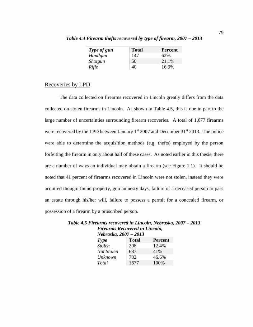
79
Table 4.4 Firearm thefts recovered by type of firearm, 2007 – 2013
Type of gun Total Percent
Handgun 147 62%
Shotgun 50 21.1%
Rifle 40 16.9%
Recoveries by LPD
The data collected on firearms recovered in Lincoln greatly differs from the data
collected on stolen firearms in Lincoln. As shown in Table 4.5, this is due in part to the
large number of uncertainties surrounding firearm recoveries. A total of 1,677 firearms
were recovered by the LPD between January 1st 2007 and December 31st 2013. The police
were able to determine the acquisition methods (e.g. thefts) employed by the person
forfeiting the firearm in only about half of these cases. As noted earlier in this thesis, there
are a number of ways an individual may obtain a firearm (see Figure 1.1). It should be
noted that 41 percent of firearms recovered in Lincoln were not stolen, instead they were
acquired though: found property, gun amnesty days, failure of a deceased person to pass
an estate through his/her will, failure to possess a permit for a concealed firearm, or
possession of a firearm by a proscribed person.
Table 4.5 Firearms recovered in Lincoln, Nebraska, 2007 – 2013
Firearms Recovered in Lincoln,
Nebraska, 2007 – 2013
Type Total Percent
Stolen 208 12.4%
Not Stolen 687 41%
Unknown 782 46.6%
Total 1677 100%

80
For the reasons mentioned above, there are many uncertainties about the origins of
firearms recovered in Lincoln. Information regarding the locations and type of recovery,
however, are not as ambiguous. Firearm recoveries are shown below in a similar fashion
to thefts, by point data and by CBGs (Figures 4.11 and 4.12). A visual analysis of Figure
4.11 reveals that firearm thefts occur all across the city with a particularly large clustering
of recoveries occurring in the downtown area. This pattern is consistent with recoveries of
firearm thefts. Figure 4.12 shows the number of firearms recovered by CBG which exhibits
a different pattern than Figure 4.11. Though there are a large number of firearms that are
recovered in the downtown area there are two CBGs that have a large number of recoveries
just west of the downtown area. This trend is most likely, in part, due to few incidents
where a large number of firearms were recovered.
Figure 4.11 Firearm Recoveries in Lincoln, Nebraska, 2007 – 2013

81
In Figure 1.1 it can be seen that there are a large number of firearm thefts that occur
along the eastern edge of the city. This trend is not reflected in the recoveries of firearms.
It is apparent from a visual analysis that very few firearms that are stolen in this area are
recovered in this area if recovered at all. Furthermore, very few firearms are recovered in
this area, whether they were stolen or not. Furthermore, less than 14 firearms were
recovered in the CBGs where 97 firearms were stolen from Scheels.
Once again there are a number of possible reasons for this change in patterns.
Property crimes, of which firearm thefts are one type, are more characteristic of areas with
middle to higher economic status. In Lincoln, criminals who most likely live in the central
and northwestern parts of the city travel to the southwestern part of the city to commit their
Figure 4.12 Firearm Recoveries in Lincoln, Nebraska by CBG, 2007 - 2013

82
crimes of theft and then return home to the central and northern parts of the city where
firearms are more commonly recovered. This trend is supported by Figure 4.10 which
shows the recoveries of firearms stolen in Lincoln.
As mentioned above, not all firearms recovered in Lincoln were involved in crimes,
much less violent crimes. Tables 4.6 and 4.7 present the statistics on firearm recoveries
and their involvement in crimes. Just over half of the 1,677 firearms recovered by the LPD
were actually involved in a crime. Over 80 percent of recovered stolen firearms by the
LPD were, however, used in crimes. In both cases, firearm use in violent crimes is just
over 10 percent. Once again, these numbers should be considered with caution because of
the large number of uncertainties regarding the origins of the firearms. These numbers
could vary greatly provided the origins for the additional 782 unknown firearms were
classified as stolen or not stolen. Furthermore, these numbers still only reflect the firearms
recovered by the LPD and do not account for any of the firearms that were never reported
or were recovered after being used in a crime. Though there are many issues with the data,
the Figures show a strong likelihood that a firearm, after being stolen, will eventually be
used in the commission of a crime, a likelihood that is much greater than firearms not
stolen.
Table 4.6 Total recoveries of firearms that were involved in crimes, 2007 – 2013
Involved in Crime Total Percent
Yes 843 50.3%
Violent 186 11.1%
No 834 49.7%
Suicide 80 4.8%
Attempted Suicide 173 10.3%
All Recoveries 1677 100%

83
Table 4.7 Total recoveries involved in crimes that were stolen, 2007 – 2013
Involved in Crime Total Percent
Yes 167 80.3%
Violent 21 10.1%
No 41 19.7%
Suicide 0 0%
Attempted Suicide 0 0%
All Stolen Recoveries 208 100%
A map of LPD recoveries of firearms used in crimes also reveal significant patterns
(Figure 4.13). A large amount of clustering can be seen around the CBD/downtown area.
This pattern is even more pronounced for recovered firearms used in violent crimes (Figure
4.14). Once again, this suggests that firearms travel into to the densely populated lower
income areas before being used in crimes and subsequently recovered by the LPD.
Figure 4.13 Firearms recovered in Lincoln, Nebraska that were used in a crime, 2007 – 2013

84
Table 4.3 and Figure 4.8 show that handguns are the most commonly stolen type
of firearm. This is consistent with other research discussed in Chapter 2 (BJS 2013, 2001;
Sheley and Wright 1993; Wright and Rossi 1986, 1994). Table 4.8 shows that handguns
are also the leading type of firearm recovered by the LPD, though each type of firearm has
a very similar spatial distribution across the city (Figure 4.15). The rate and distribution
of handgun recovery both suggest that handguns are, by far, used much more in crimes.
This is most likely explained by their concealable and lightweight nature in addition to
having a low cost of operating.
Table 4.8 Firearms recovered in Lincoln, Nebraska by type of firearm, 2007 – 2013
Type Total Percent
Handgun 803 47.9%
Shotgun 396 23.6%
Figure 4.14 Firearms Recovered in Lincoln, Nebraska that were used in a Violent Crime, 2007 – 2013

85
Rifle 478 28.5%
Maps portraying firearms recovered in Lincoln that were stolen (Figures 4.16 and
4.17) show a very similar pattern to firearms stolen and recovered in Lincoln. This is to be
expected considering 181 of the 208 recovered stolen firearms were stolen in Lincoln.
Furthermore, 27 of the firearms recovered in Lincoln were not stolen in Lincoln, which is
significantly less than the 56 stolen in Lincoln and recovered elsewhere. More firearms
are stolen and trafficked out of Lincoln than are stolen and trafficked into Lincoln. Most
firearms that stay in Lincoln are recovered in the downtown area. The most reasonable
explanation for this is that the supply of firearms in Lincoln is greater than the demand,
while the demand for firearms, at least for criminal use, is much greater in other parts of
the country (see also Figure 4.18).
Figure 4.15 Firearm Recoveries in Lincoln, Nebraska by Type of Firearm, 2007 - 2013

86
Figure 4.16 Firearms recovered in Lincoln, Nebraska that were stolen, 2007 - 2013
Figure 4.17 Firearms recovered in Lincoln, Nebraska that were stolen by CBG, 2007 – 2013

87
The ANN analysis showed a significant amount of clustering for all four point
datasets: (1) firearms thefts (from the stolen firearms dataset), (2) firearm thefts recovered
(from the stolen recovered dataset), (3) firearm recoveries (from the recovered firearms
dataset), and (4) firearms recoveries that were stolen (from the recovered stolen dataset);
(Table 4.9). This reflects the fact that more than one firearm is frequently involved in the
theft or recovery. Conversely, results from the spatial autocorrelation analysis of the four
polygon distributions revealed that only recoveries were clustered, while the distribution
of thefts was random (Table 4.10). These results suggest that thefts of firearms in CBGs
are not related to the thefts of firearms in adjoining CBGs. Conversely, the recovery of
firearms, both stolen or not, are spatially autocorrelated to themselves in the adjoining
CBGs.
Table 4.9 Average Nearest Neighbor Results
Dependent
variable
Observed
Mean Distance
Expected Mean
Distance
ANN Ratio z-score p-value
Stolen Firearms 354.9174 1002.9080 0.353888 -33.464974 0.0000
Stolen Recovered 44,082.3786 22,3150.8220 0.197545 -23.633368 0.0000
Recovered 253.0976 709.3630 0.356796 -50.390238 0.0000
Recovered Stolen 880.5484 1849.5897 0.476078 -14.455377 0.0000
Table 4.10 Spatial Autocorrelation Results
Dependent
variable
Moran’s Index Expected Index Variance z-score p-value
Stolen Firearms -0.011578 -0.005376 0.000885 -0.208501 0.834838
Stolen Recovered 0.113863 -0.005376 0.001063 3.657562 0.000255
Recovered 0.246772 -0.005376 0.001655 6.197899 0.000000
Recovered Stolen 0.101106 -0.005376 0.001152 3.136699 0.001709

88
Gang Theft Statistics
Between January 1st 2007 and December 31st 2013, there were a total of 22 gang
thefts involving the taking of firearms (Table 4.11). The average theft in Lincoln regardless
of gang involvement was 1.9 firearms per theft, which is significantly lower than the
average for gang involvement at 6.6 firearms per theft. Tables 4.12 and 4.13 present a
comparison of the statistics for firearm thefts recovery by location, both involving and
indifferent to gang activity. Figure 4.18 shows that all firearms stolen and trafficked out
of Nebraska traveled southwest. The map shows the States firearms were recovered in
after being stolen in Lincoln. Furthermore, the map specifically shows, in addition to the
previous map elements, the movement of stolen firearms due to gang activity.
One possible explanation is that gangs in Lincoln have close relations to gangs in
Phoenix, AZ. Another possible explanation is that a gang based out of Phoenix has
branched out to Lincoln. An alternative explanation would be that these stolen firearms
are being smuggled into Mexico and Arizona is the preferred state border to cross. One
study found that since 2004, gun seizures have dramatically increased along with gun
violence along the Arizona/Mexico border (Dube, et al 2013).
Table 4.11 General descriptive data for gang thefts in Lincoln, Nebraska, 2007 – 2013
Measure Value
Firearms Stolen 146
Firearm Thefts 22
Average # of Firearms Stolen per Theft 6.64
Average Value of Stolen Firearm $380.12
Thefts where Firearm was the target 112
Total Stolen Firearms Recovered 96
Recovered in Lincoln 72
Recovered outside of Lincoln 24

89
Table 4.12 Gang thefts recovered by
location,
2007 – 2013
Location Total
Lincoln 72
Nebraska 80
Arizona 13
California 2
Colorado 1
Mean Distance 169.1 miles
Median Distance 4.9 miles
Range 0 – 1382.5 miles
Table 4.13 Stolen firearms recovered by
location of recovery, 2007 – 2013
Location Total
Lincoln 179
Nebraska 214
Arizona 13
California 3
Colorado 2
Illinois 1
Iowa 1
Kentucky 1
South Dakota 1
Washington 1
Mean Distance 27.8 miles
Median Distance 4.24 miles
Range 0 – 1382.5 miles
Figure 4.18 National recovery map of firearms stolen in Lincoln, Nebraska, 2007 – 2013

90
Objective 3
Spatial analysis of Thefts and Recoveries over time
The third objective for this study is to examine and possibly explain the change in
the spatial patterns of firearm thefts and recoveries over time. All crime, violent crime,
and property crime patterns were mapped in addition to firearm thefts and recoveries for
each year during the study period. These maps are presented below in Figures 4.19, 4.20,
4.21, 4.22, 4.23, 4.24, and 4.25.
It is noteworthy that all crime, including violent and property crime, predominantly
occurred in the north central and downtown areas of Lincoln in each year. The southeast
part of the city either exhibited insignificant levels of crime or, in many cases is shown as
a Cold Spot, which signifies that an area has lower crime levels.
Firearm thefts have a large amount of variation in spatial patterns from year to year.
These large discrepancies from year to year can most likely be explained by one of the
following reasons. First, firearm thefts in Lincoln occur far less often when compared to
other crime types. Though the theft of firearms is very much an opportunistic crime, the
opportunities to commit the crime comes far less often. Furthermore, because of the
infrequency of opportunities to steal a firearm, spatial patterns are greatly affected by single
incidents where a large number of firearms are acquired. Another possible explanation
suggests that criminals change their target territories over time. For this reason, criminals
may target an area for a limited period of time before moving on to another area so as to
avoid arrest.

91
Firearm recoveries occur mostly in downtown Lincoln. This area of Lincoln is
more densely populated, has a greater prevalence of firearms, and the area just south and
west of the downtown area is generally subject to higher levels of other crime types
suggesting a greater concentration of criminals. Finally, results from mapping Lincoln
with socio-economic data shows that this area is less economically stable maintaining
lower levels of income. These findings are consistent with other research discussed in
chapter 2 (Altheimer 2008; Altheimer and Boswell 2011; Hoskin 2006).
Figure 4.19 Hot and Cold Spot Analyses of Firearm Thefts and Recoveries, All Crimes, Violent
Crimes, and Property Crimes in Lincoln, Nebraska in 2007

92
Figure 4.21 Hot and Cold Spot Analyses of Firearm Thefts and Recoveries, All Crimes, Violent
Crimes, and Property Crimes in Lincoln, Nebraska in 2009
Figure 4.20 Hot and Cold Spot Analyses of Firearm Thefts and Recoveries, All Crimes, Violent Crimes,
and Property Crimes in Lincoln, Nebraska in 2008

93
Figure 4.23 Hot and Cold Spot Analyses of Firearm Thefts and Recoveries, All Crimes, Violent
Crimes, and Property Crimes in Lincoln, Nebraska in 2011
Figure 4.22 Hot and Cold Spot Analyses of Firearm Thefts and Recoveries, All Crimes, Violent
Crimes, and Property Crimes in Lincoln, Nebraska in 2010

94
Figure 4.24 Hot and Cold Spot Analyses of Firearm Thefts and Recoveries, All Crimes, Violent
Crimes, and Property Crimes in Lincoln, Nebraska in 2012
Figure 4.25 Hot and Cold Spot Analyses of Firearm Thefts and Recoveries, All Crimes, Violent
Crimes, and Property Crimes in Lincoln, Nebraska in 2013

95
Objective 4
Correlation
Correlation matrices were constructed for each dependent variable to determine the
strength of the relationships between firearm thefts and recoveries. Both stolen and
recovered firearms had a significant relationship with the logged transformation of the gun-
related crime rate. Furthermore, results from the t-test were significant enough to reject
the null hypotheses that these correlations were equal to zero. Though firearm recoveries
did have a significant relationship with the transformed violent crime variable, firearm
thefts did not. Results from the t-test were strong enough to reject the null hypothesis that
the relationship between firearm recoveries and the dependent variable were equal to zero.
Finally, both firearm thefts and recoveries were significantly correlated with the
transformed property crime variable. Results from the t-test were significant enough to
reject the null hypotheses that either variable’s correlation with the dependent variable was
equal to zero.
Dependent variable = log of the gun-related crimes rate
Independent variables = stolen firearm and the recovered firearm rates
STLN_R RCVD_R LOG_Gun_R
STLN_R 1
RCVD_R 0.275286 1
LOG_Gun_R 0.231274 0.396207 1
STLN t-test = 3.2333201 (rejected the null hypothesis that r = 0)
RCVD t-test = 5.869346 (rejected the null hypothesis that r = 0)

96
Dependent variable = log of violent crime
Independent variable = stolen firearms and recovered firearms raw count data
STLN RCVD Log_Violent
STLN 1
RCVD 0.194294 1
Log_Violent 0.112032 0.515835 1
STLN = not significant (failed to reject null hypothesis that r = 0)
RCVD t-test = 8.18982 (rejected the null hypothesis that r = 0)
Dependent variable = log of property crime
Independent variable = stolen firearms and recovered firearms raw count data
STLN RCVD Log_Property
STLN 1
RCVD 0.194294 1
Log_Property 0.235585 0.500184 1
STLN t-test = 3.297101 (rejected the null hypothesis that r = 0)
RCVD t-test = 7.856663 (rejected the null hypothesis that r = 0)
Spatial Autocorrelation
Spatial autocorrelation was performed on each dependent variable to determine if,
in fact, the variable was related to itself over space (Table 4.14). Results for each variable
were significant and revealed that each variable was spatially autocorrelated. Spatially
autocorrelated variables imply that levels of crime are, in part, affected by the levels of that
crime over space. This analysis also resulted in the residuals of the subsequent OLS
regression tests being spatially autocorrelated. Spatially autocorrelated residuals indicated
that the spatial dependence of the dependent variable should be accounted for as an

97
explanatory variable and was therefore accounted for in the MLE test performed in Geoda
in the next step.
Table 4.14 Spatial Autocorrelation Results
Dependent variable Moran’s Index Expected Index Variance z-score p-value
Gun-related crimes 0.304890 -0.005376 0.001655 7.625809 0.00000
Violent crimes 0.386611 -0.005376 0.001687 9.543685 0.00000
Property crimes 0.259477 -0.005376 0.001619 6.582770 0.00000
Regression
Regression analysis was conducted using three different models: (1) Gun-related
crimes (Model 1), (2) Violent crimes (Model 2), and (3) Property crimes (Model 3).
Results from the initial analyses indicated that each of the models had residuals that were
spatially auto-correlated. As a result the models had to be re-run without a cutoff for spatial
autocorrelation and Jarque Bera in order to discern the best model. Furthermore, each
model subsequently had to be tested in a MLE model in order to discern if the spatial
component was, in fact, a key variable missing from the initial classic OLS model. The
results are discussed by model below.
Model 1: Gun-related crimes
Results from the OLS model 1 revealed that the sum of the rates for stolen firearms,
drug crimes, dropouts, and broken homes were the best fit model with an R2 = 0.35. The
model was subsequently tested using classic OLS in Geoda and revealed the same R2. The
fit of the model is not that impressive, however it is statistically significant and positive,
indicating that the combination of the select independent variables can explain as much as

98
35 percent of the variance in gun-related crimes. Results from the VIF test suggested that
multicollinearity is not an issue with this model. Furthermore, results from the Moran’s I
spatial autocorrelation test indicated that spatial regression was likely an issue that had not
been accounted for with the simple OLS model. The diagnostic of spatial dependence
revealed that only the Lag model was significant. Furthermore, in the robust model, only
the Lag model was significant with a p-value of 0.0286021. The model was then tested
using the Spatial Lag and Spatial Error (MLE) models in Geoda. The log likelihood was
used to compare the results of these three tests to discern the strongest model (Table 4.15).
As suggested from the results in the Moran’s I test in the previous step, a comparison of
the log likelihood values reveals that the Lag model shows the greatest amount of
improvement. The Lag model indicates that the incidents of gun-related crime will impact
the likelihood that more gun-related crime will occur.
Table 4.16 shows the parameter estimates. The coefficients or b values indicate
the direction and number of units (as coded) of change in the dependent variable
due to a one unit change in each independent variable (University of Toronto 2014).
Individually the independent variables have very small coefficients, explaining only a
minute amount of the slope. The results do show, however, that the dependent variable
will change by about .29 units in the same direction due to one unit change in the Lag
coefficient (Table 4.17), while a change of about .28 units will occur with the Lambda
coefficient from the Error model (Table 4.18). Results from the t-Statistic indicate that the
null hypothesis that the slope is equal to zero can be rejected.

99
When controlling for the spatial component of gun-related crimes, a one unit
increase in gun-related crimes produces about a third unit increase (+.29) in gun-related
crime. A crime involving a gun, for example, is more likely to occur in an area where three
or four gun-related crimes have already occurred. When controlling for the spatial
component of Lambda, a one unit increase in a variable unaccounted for produces about a
third unit increase (+.28) in gun-related crime. A crime involving a gun, for example, is
more likely to occur in an area where three or four incidents of an unknown variable have
already occurred. A complete report is available in the appendix (page 137).
Table 4.15 Results from model 1 for Ordinary Least Squares, Spatial Lag, and Spatial
Error regression models
Method Log Likelihood
OLS -291.195
Spatial Lag -287.356
Spatial Error -289.066881
Table 4.16 Parameter estimates for OLS model 1
Variable Coefficient Standard Error t-Statistic Probability
CONSTANT 4.886895 0.1613671 30.2843 0.0000000
STLN_R 0.00041825 0.000152986 2.73389 0.006877
CRIMES_DRUGS 4.57E-05 7.90E-06 5.78542 0.0000000
DROPOUT_R 3.64E-05 1.31E-05 2.77774 0.006048
BROKEN_HOMES 1.92E-05 5.29E-06 3.63823 0.000357
Table 4.17 Parameter estimates for spatially lagged model 1
Variable Coefficient Standard Error z-value Probability
W_LOG_GUN_R 0.2899464 0.09288913 3.121425 0.0017999
CONSTANT 3.320052 0.5294989 6.270178 0.0000000
STLN_R 0.0004365976 0.0001469326 2.971414 0.0029645
CRIMES_DRUGS 3.89822e-005 8.04669e-006 4.844501 0.0000013
DROPOUT_R 2.389022e-005 1.298356e-005 1.840037 0.0657627
BROKEN_HOMES 1.585289e-005 5.110174e-006 3.102222 0.0019209

100
Table 4.18 Parameter estimates for spatial error model 1
Variable Coefficient Standard Error z-value Probability
CONSTANT 4.998515 0.187069 26.72016 0.0000000
STLN_R 0.0003937612 0.0001468474 2.681432 0.0073309
CRIMES_DRUGS 4.75829e-005 8.317203e-006 5.721022 0.0000000
DROPOUT_R 2.994183e-005 1.3167e-005 2.274006 0.0229656
BROKEN_HOMES 1.556293e-005 5.154881e-006 3.019066 0.0025357
LAMBDA 0.2792174 0.107676 2.593127 0.0095108
Model 2: Violent Crimes
Results from the OLS model 2 revealed that the sum of recovered firearms, crimes
involving drugs, and broken homes were the best fit model with an R2 = 0.52. The model
was subsequently tested using classic OLS in Geoda and revealed the same R2. The fit of
the model is more impressive than model 1, statistically significant, and positive, indicating
that the combination of the select independent variables can explain as much as 52 percent
of the variance in gun-related crimes. Results from the VIF test suggested that
multicollinearity is not an issue with this model. Furthermore, results from the Moran’s I
spatial autocorrelation test indicated that spatial regression was likely an issue that had not
been accounted for with the simple OLS model. The diagnostic of spatial dependence
revealed that both the Lag and the Error models were significant, however, only the robust
Error model was significant with a p-value of 0.0114795. The model was then tested using
the Spatial Lag and Spatial Error (MLE) models in Geoda. The log likelihood was used to
compare the results of these three tests to discern strongest model (Table 4.19). As
suggested from the results in the Moran’s I test in the previous step, a comparison of the
log likelihood values reveals that the Error model shows the greatest amount of

101
improvement. The Error model indicates that the occurrence of a variable unaccounted for
in the model will impact the likelihood that more violent crime will occur.
Table 4.20 shows the parameter estimates. Individually, all of the independent
variables except broken homes have very small coefficients, explaining only a minute
amount of the slope. A one unit increase in broken homes produces a 1.5 unit increase in
violent crime. An area may be subject to three additional violent crimes for every unit
increase in broken homes. In addition, the results show that the dependent variable will
change by about .27 units in the same direction due to one unit change in the Lag coefficient
(Table 4.21), while a change of about .44 units will occur with the Lambda coefficient from
the Error model (Table 4.22). Results from the t-Statistic indicate that the null hypothesis
that the slope is equal to zero can be rejected.
When controlling for the spatial component of violent crime, a one unit increase in
violent crimes produces about a quarter unit increase (+.27) in violent crime. When
controlling for the spatial component of Lambda, a one unit increase in a variable
unaccounted for produces just under a half unit increase (+.44) in violent crime. A
complete report is available in the appendix (page 155).
Table 4.19 Results from model 2 for Ordinary Least Squares, Spatial Lag, and Spatial
Error regression models
Method Log Likelihood
OLS -197.988
Spatial Lag -192.301
Spatial Error -189.714089
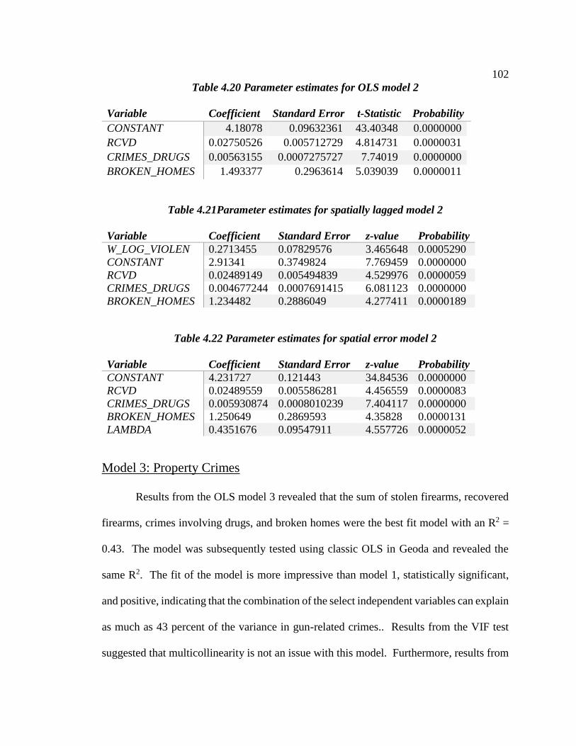
102
Table 4.20 Parameter estimates for OLS model 2
Variable Coefficient Standard Error t-Statistic Probability
CONSTANT 4.18078 0.09632361 43.40348 0.0000000
RCVD 0.02750526 0.005712729 4.814731 0.0000031
CRIMES_DRUGS 0.00563155 0.0007275727 7.74019 0.0000000
BROKEN_HOMES 1.493377 0.2963614 5.039039 0.0000011
Table 4.21Parameter estimates for spatially lagged model 2
Variable Coefficient Standard Error z-value Probability
W_LOG_VIOLEN 0.2713455 0.07829576 3.465648 0.0005290
CONSTANT 2.91341 0.3749824 7.769459 0.0000000
RCVD 0.02489149 0.005494839 4.529976 0.0000059
CRIMES_DRUGS 0.004677244 0.0007691415 6.081123 0.0000000
BROKEN_HOMES 1.234482 0.2886049 4.277411 0.0000189
Table 4.22 Parameter estimates for spatial error model 2
Variable Coefficient Standard Error z-value Probability
CONSTANT 4.231727 0.121443 34.84536 0.0000000
RCVD 0.02489559 0.005586281 4.456559 0.0000083
CRIMES_DRUGS 0.005930874 0.0008010239 7.404117 0.0000000
BROKEN_HOMES 1.250649 0.2869593 4.35828 0.0000131
LAMBDA 0.4351676 0.09547911 4.557726 0.0000052
Model 3: Property Crimes
Results from the OLS model 3 revealed that the sum of stolen firearms, recovered
firearms, crimes involving drugs, and broken homes were the best fit model with an R2 =
0.43. The model was subsequently tested using classic OLS in Geoda and revealed the
same R2. The fit of the model is more impressive than model 1, statistically significant,
and positive, indicating that the combination of the select independent variables can explain
as much as 43 percent of the variance in gun-related crimes.. Results from the VIF test
suggested that multicollinearity is not an issue with this model. Furthermore, results from

103
the Moran’s I spatial autocorrelation test indicated that spatial regression was likely an
issue that had not been accounted for with the simple OLS model. The diagnostic of spatial
dependence revealed that both the Lag and the Error models were significant, however,
only the Robust Error model was significant with a p-value of 0.0030975. The model was
then tested using the Spatial Lag and Spatial Error (MLE) models in Geoda. The log
likelihood was used to compare the results of these three tests to discern the strongest model
(Table 4.23). As suggested from the results in the Moran’s I test in the previous step, a
comparison of the log likelihood values reveals that the Error model shows the greatest
amount of improvement. The Error model indicates that the occurrence of a variable
unaccounted for in the model will impact the likelihood that more property crime will
occur.
Table 4.24 shows the parameter estimates. Individually, all of the independent
variables except broken homes have very small coefficients, explaining only a minute
amount of the slope. A one unit increase in broken homes produces a .9 unit increase in
violent crime. In addition, the results show that the dependent variable will change by
about .25 units in the same direction due to one unit change in the Lag coefficient (Table
4.25), while a change of about .46 units will occur with the Lambda coefficient from the
Error model (Table 4.26). Results from the t-Statistic indicate that the null hypothesis that
the slope is equal to zero can be rejected.
When controlling for the spatial component of property crime, a one unit increase
in property crimes produces about a quarter unit increase (+.25) in property crime. When
controlling for the spatial component of Lambda, a one unit increase in a variable

104
unaccounted for produces just under a half unit increase (+.46) in property crime. A
complete report is available in the appendix (page 173).
Table 4.23 Results from model 3 for Ordinary Least Squares, Spatial Lag, and Spatial
Error regression models
OLS, Spatial Lag, and Spatial Error model 3 results
Method Log Likelihood
OLS -189.413
Spatial Lag -185.841
Spatial Error -181.355665
Table 4.24 Parameter estimates for OLS model 3
Variable Coefficient Standard Error t-Statistic Probability
CONSTANT 5.183483 0.09460903 54.78846 0.0000000
STLN 0.01906406 0.006189306 3.080162 0.0023898
RCVD 0.02346362 0.005585909 4.200501 0.0000417
CRIMES_DRUGS 0.004237366 0.0006973035 6.076789 0.0000000
BROKEN_HOMES 0.900852 0.2845724 3.165634 0.0018144
Table 4.25 Parameter estimates for spatially lagged model 3
Variable Coefficient Standard Error z-value Probability
W_LOG_PROPER 0.2498655 0.08538083 2.926482 0.0034283
CONSTANT 3.754025 0.4864078 7.717854 0.0000000
STLN 0.01913044 0.005964895 3.207171 0.0013406
RCVD 0.02145485 0.005434157 3.948148 0.0000788
CRIMES_DRUGS 0.003700371 0.000720389 5.136629 0.0000003
BROKEN_HOMES 0.7850441 0.2770955 2.833118 0.0046098
Table 4.26 Parameter estimates for spatial error model 3
Variable Coefficient Standard Error z-value Probability
CONSTANT 5.133351 0.1198003 42.84922 0.0000000
STLN 0.0157311 0.005598717 2.809768 0.0049578
RCVD 0.02250005 0.005419347 4.151802 0.0000330
CRIMES_DRUGS 0.00491286 0.0007717523 6.36585 0.0000000
BROKEN_HOMES 0.8724605 0.2742392 3.181386 0.0014659
LAMBDA 0.4619714 0.09307363 4.963504 0.0000007

105
Discussion of Statistical Results
Results from the correlation matrices revealed that firearms recovered in Lincoln
were significantly related to each of the three dependent variables: (1) Gun-related crimes
(Model 1), (2) Violent crimes (Model 2), and (3) Property crimes (Model 3). Firearm
thefts, however, were only significantly correlated with gun-related crimes and property
crimes, not violent crimes. The Spatial Autocorrelation tests indicated that all three
dependent variables were in fact related to themselves over space. This, in turn, lead to
biased results when the exploratory regression tool was executed, indicating that a key
explanatory variable (the spatial component of the dependent variable), was missing from
the equation. Subsequent regression analyses revealed significant results for each model
without accounting for spatial autocorrelation of the residuals. The most significant results
from each model were chosen and analyzed with the Geoda software. Results from the
regression analysis in Geoda indicated that the spatial autocorrelation of the dependent
variable was an issue that had to be accounted for. As a result, subsequent MLE analyses
for each model yielded improved results implying that the dependent variables have a
significant impact on themselves over space.
Recovered firearms explained, in part, the slope of all three models and stolen
firearms were used to explain, in part, the slope of both gun-related and property crimes.
Drug-related crimes were also found to be significantly related to all three models and
explain part of the variance in each of the dependent variables. The literature review
suggested that five measures that have been used in previous research to explain or attempt
to explain crime: (1) age (youth), (2) race (minority), (3) education (dropout), (4) wealth

106
(poverty), and (5) homes stability (broken homes) (Altheimer 2010, 2008; Altheimer and
Boswell 2011; ATF 2000; Braga and Kennedy 2001; BJS 2013; Cohen and Tita 1999;
Cook and Ludwig 2004; Hoskin 2006; Lochner and Moretti 2001; Rosenfeld 1999;
Sampson 1986, and 1987; Sheley and Wright 1993; Stolzenberg and D’Alessio 2000; Sun,
Triplett, and Gainey 2004). In all three models, the measure for broken homes was
significantly related to and helped explain, in part, the variance of the dependent variables.
The measure for dropout was significantly related to and helped, in part, explain the
variance of the dependent variable for model 1, gun-related crimes. Surprisingly, the
measures for youth, minorities, and poverty were not important in the most significant
models. Conversely, the youth variable had a very negative effect in all three models.
Though the models did improve, they are not perfect, therefore, other variables must be
missing that were not accounted for. These variables could be different measures from
those used in this study such as, other demographic, social, and natural variables not
accounted for in this study, true spatial dependence, or most likely, a combination of more
than one missing variable.
Key Findings
The results reported on in this chapter addressed four main objectives; 1) how
firearm thefts are spatially distributed in Lincoln, Nebraska, a typical medium-size U.S.
city, (2) where firearms are recovered in Lincoln, (3) if the spatial distributions of firearm
thefts and recoveries have changed over the study period 2007-2013, and (4) whether the
spatial distributions of firearm thefts and/or recoveries are related to spatial patterns of

107
other crimes and/or socio-demographic characteristics (e.g., income, age or ethnicity) of
Lincoln’s populace.
Both the volume of firearms stolen and recovered in Lincoln were larger than
anticipated. Lincoln has, on average, 1.9 firearms stolen per theft which is very close to
Kleck’s (2009) finding of 2.2 firearms per theft. The data also showed, however, that, on
average, over 6.5 firearms are stolen per gang theft. These results clearly indicate that
firearm theft is related to gang activity. The results also revealed that firearm recoveries
were close to locations of thefts. Though most firearms stolen in Lincoln were also
recovered in Lincoln, a small, but significant number of firearms involved with gangs were
recovered in southwestern states, especially in Phoenix, Arizona.
Handguns are stolen in Lincoln more than any other type of firearm. Furthermore,
handguns are more likely to be used in the commission of a crime in Lincoln than any other
type of firearm. These results support the national data reported by the BJS (2013).
Furthermore, the results also indicated that firearm thefts occur predominantly in
residential areas. These results are also supported by the BJS (2013) and Kleck (2009).
The major objective of this thesis was to discern if firearm thefts and/or recoveries
were spatially clustered. The results indicated that they were in Lincoln. Due to the lack
of research regarding the spatial component of firearm thefts, these results cannot be
compared to other studies, however they do suggest that firearm thefts are concentrated
much like other crimes (Braga et al 2010).
Statistical analyses showed that firearm thefts and recoveries were significantly
related to both gun-related and property crimes. Unlike firearm recoveries, firearm thefts

108
were not significantly related to violent crime. Furthermore, drug-related crimes were also
significantly related to all three variables: gun-related crimes, violent crimes, and property
crimes. The results also suggest that broken homes are significantly related to all three
dependent variables, which is consistent with previous research (Altheimer 2010; Sampson
1986, and 1987; Sun, Triplett, and Gainey 2004).
Finally, results from the MLE Spatial Lag and Spatial Error analyses revealed an
improvement in the slope of all three dependent variables. Specifically, model 1 revealed
the greatest amount of improvement came with the Spatial Lag estimation suggesting that
gun-related crime greatly influences the gun-related crimes in other CBGs. Conversely,
the Spatial Error model showed the greatest improvement for models 2 and 3 suggesting
that the clustering of an unknown explanatory variable was greatly affecting the slope of
both property and violent crimes. It should be noted that the Spatial Lag estimations also
improved both of these models suggesting that the dependent variables did influence the
dependent variables in adjoining CBGs, however, there were other significant variables not
accounted for such as true spatial dependence and other variables not used in this study.
These results were expected considering all three dependent variable were spatially auto
correlated. Ultimately, more research needs to be conducted to verify these conclusions,
however, spatial dependence most certainly contributes to the occurrence of crime
throughout Lincoln. Most interestingly, firearm thefts did not affect crime as much as
originally suspected.

109
Conclusion
This chapter presented the results of statistical analyses. Results revealed that
firearm thefts and recoveries are clustered in the city of Lincoln. Hot Spot analyses over
time revealed that the clustering of firearm thefts changed dramatically from year to year.
Furthermore, the clustering of firearm recoveries was more consistent than the clustering
of firearm thefts. Clustering patterns for violent, property, and all crimes showed the most
stability around the city from year to year. Finally, statistically significant relationships
were discovered to exist between gun-related and property crimes. Moreover, firearm
recoveries, unlike thefts, were significantly related to violent crimes in addition to gun-
related and property crimes. Chapter five presents a summary of this thesis, a suggested
interpretation of the results, and possible directions for future research.

110
Chapter 5: Conclusion
Summary
Firearm use and regulation in the United States is of great concern to many and
constantly the center of many debates. Firearm use is greatly associated with illegal
activities to include violent and property crimes. Many studies have indicated that violent
crimes tend to increase when firearms are abundantly available, both legitimate and/or
illicit, and are easily obtained (Altheimer 2010; Cook and Ludwig 2004; Hoskin 2001;
Stolzenberg and D'Alessio 2000; McDowall 1991; Cook 1983) though other studies have
found no apparent correlation (Altheimer 2008; Kates and Mauser 2007; Kleck and
Patterson 1993). Virtually all investigators agree, however, that stolen firearms account for
a large percentage of firearms used in violent crimes and firearms in general account for a
large percentage of violent crimes committed in the United States. Because of
shortcomings in data, there has been little research on the spatial dimensions of firearm
theft, firearm trafficking, and their relation to crime, especially at the local level. This
thesis seeks to expand the understanding of gun theft by using GIS and statistical tools to
analyze improved information about such issues.
Objectives Restated
This thesis attempted to address the issue of firearm thefts in addition to examining
their relationship with other crime types. The study examined data collected on firearm
thefts and recoveries in Lincoln, Nebraska. The principal objectives of this research were

111
to determine (1) how firearm thefts are spatially distributed in Lincoln, Nebraska, a typical
medium-size U.S. city, (2) where firearms are recovered in Lincoln, (3) if the spatial
distributions of firearm thefts and recoveries have changed over the study period 2007-
2013, and (4) whether the spatial distributions of firearm thefts and/or recoveries are related
to spatial patterns of other crimes and/or socio-demographic characteristics (e.g., income,
age or ethnicity) of Lincoln’s populace. A GIS and geospatial statistics are used to identify
hotspots of firearm theft and recovery and to explore relationships between such events,
other crimes and socio-demographic variables.
Objectives 1 and 2
Several maps, Tables, and Figures were created to determine if firearm thefts and
recoveries were clustered in Lincoln. Numerous point, choropleth, and maps were
generated to display the different types of clustering for firearm thefts in Lincoln, firearms
stolen and recovered in Lincoln, firearms recovered in Lincoln, and firearms recovered in
Lincoln that were stolen. Initial map and spatial statistical analyses revealed the firearm
thefts and recoveries were, in fact clustered within Lincoln, particularly in the CBD. The
ANN analyses revealed that the locations and the number of firearms stolen or recovered
for all four datasets were spatially clustered. Results from the Spatial Autocorrelation
Analyses revealed that only the recoveries of firearms were clustered based on the data
aggregated to CBGs.

112
Objective 3
Thirty maps were created using the Getis Ord Hot Spot analysis method to
determine the amount of change in spatial patterns of firearm thefts and recoveries. The
maps were organized into seven Figures and display the Hot Spot distributions of firearm
thefts, recoveries, all crimes, violent crimes, and property crimes by year between 2007
and 2013. The analyses revealed that the clustering of firearm thefts vary more than firearm
recoveries from year to year. These results suggest that though firearm thefts do tend to
cluster, the locations will vary over time.
Objective 4
Additional statistical analyses using Correlation matrices, t-tests, OLS, and MLE were
conducted to determine the relationships firearm thefts and recoveries had with gun-
related, violent, and property crime in Lincoln. Results suggested that both firearm thefts
and recoveries were significantly related to all three variables, firearm thefts, however,
were not significantly related to violent crime. The relationship between firearm thefts and
violent crime was unexpected and contrary to the initially anticipated results. Considering
the relationship between firearm thefts and gun-related crimes, the data suggests that
further analysis may reveal a significant relationship between firearm thefts and violent
crimes involving a firearm. Finally, In addition to the prevalence of broken homes, drug
crimes were significantly related to all three models.

113
Limitations
No previous studies have been conducted on the clustering of firearm thefts in cities
across the United States. For this reason comparing the results of this research to that of
others is difficult. This research should be considered a starting point for more research
focusing on other cities. The data collected in this research are directly taken from LPD
case files. Data were collected for the purpose of this research and may not be compatible
with future studies. Furthermore, firearm thefts not reported to the LPD were not reported
and therefore not used in this study. Firearm thefts and recoveries were used as explanatory
variables in the statistical models in an attempt to explain other crime types. Future
research may wish to use other explanatory variables to explain firearm thefts and
recoveries such as different measures from those used in this study in addition to other
demographic, social, and natural variables not accounted for in this study, true spatial
dependence, or most likely, a combination of more than one missing variable.
Implications
This study has resulted in an improved understanding of the geography of firearm theft,
recovery, and their relationships with crimes in Lincoln. This research may provide law
enforcement agencies with better analytical tools and methodologies needed to help abate
firearm theft, enhance interdiction of stolen firearms and reduce crime. This research
should be considered an initial exploratory study, inspired, but not defined by other studies.
For this reason, this research should be used to encourage others to take up similar studies
examining the spatiality of firearm thefts, recoveries, and their relationship with other

114
crimes. This research has also set an example of how to collaborate with local police to
collect and analyze data.
Though the data aggregation process was extremely time consuming, it was very
revealing. It clearly shows the importance for gun owners to properly secure their firearms.
Over half of the firearms stolen in Lincoln are taken from a residential setting.
Furthermore, a quarter of firearms are stolen from automobiles. The vast majority of
firearm thefts could be prevented if proper security measures were in place. If there is any
suggestion to be made by this research it is to highlight the importance of protecting
personal property, to include firearms, from theft. This research suggests that gang
members place a higher importance on obtaining stolen firearms and indicates that they
will go to greater lengths to obtain them. In most cases, a business was the target of gang
thefts, resulting in many firearms being stolen. Preventing the thefts is more difficult in
these situations, however tracing their movement has revealed a strong south west
movement of stolen firearms indicating a possible relationship between gang activity and
firearms trafficking. This may be a revealing study for future research.
Suggested Future Research
Additional research is needed on firearm thefts and recoveries. Future studies
should focus on the spatial distributions of firearm thefts and recoveries in other locations
similar to Lincoln, and should address specific patterns discovered from this research in
Lincoln in more depth.

115
It also is important to learn more about the circumstances under which firearms are
stolen and recovered. Researching stolen and recovered firearms is hampered by poor
communication between police departments. There are over 1,700 police agencies in the
United Sates collecting data, each in its own way. Currently there is no congruent way of
collecting data. Furthermore, though many police departments utilize advanced computer
systems for disseminating data, others still employ basic non digital reporting systems.
Improving the way data are collected and shared will ultimately lead to more
comprehensive data which in turn will provide more accurate results in subsequent studies.
Collecting data on socio, politico, and economic demographics may aid in future analyses.
Finally, this research used firearm thefts and recoveries as explanatory variables in an
attempt to help explain the variance of the dependent variables gun-related, violent, and
property crimes. Future research should be focused on explaining the variance of firearm
thefts and recoveries using other explanatory variables such as different measures from
those used in this study in addition to other demographic, social, and natural variables not
accounted for in this study, true spatial dependence, or most likely, a combination of more
than one missing variable.

116
List of References
Altheimer, Irshad, 2010. An Exploratory Analysis of Guns and Violent Crime in a Cross-
National Sample of Cities. Southwest Journal of Criminal Justice, 6(3): 204-227.
———. 2008. Do Guns Matter? A Multi-level Cross-National Examination of Gun
Availability on Assault and Robbery Victimization. Western Criminology Review,
9(2): 9–32.
Altheimer, Irshad, and Mathew Boswell. 2011. Reassessing the Association between Gun
Availability and Homicide at the Cross-National Level. American Journal of
Criminal Justice, 37: 682-704.
ArcGIS. 2013. World Geocoding.
http://www.arcgis.com/home/item.html?id=305f2e55e67f4389bef269669fc2e284
(Accessed May 21, 2014).
Arkin, Herbert, and Raymond R. Colton. 1964. Tables For Statisticians: Second Edition.
NY: Barnes and Noble.
ASU. 2014. GeoDa Center For Geospatial Analysis and Computation.
http://geodacenter.asu.edu/ (Accessed April 23, 2014).
Boba, Rachel. 2001. Introductory Guide to Crime Analysis and Mapping. Report to the
Office of Community Oriented Policing Services Cooperative Agreement #97-CK-
WXK-004.
Brady Campaign. 2013. Brady Campaign to Prevent Gun Violence.
http://www.bradycampaign.org/ (Accessed November 9, 2013).
Braga, Anthony, A., and David M. Kennedy. 2001. The Illicit Acquisition of Firearms by
Youth and Juveniles. Journal of Criminal Justice 29: 379-388.
Braga, Anthony, A., Andrew V. Papachristos, and David M. Hureau. The Concentration
and Stability of Gun Violence at Micro Places in Boston, 1980-2008. Journal of
Quantitative Criminology, 26: 33-53
Braga, Anthony A., Garen J. Wintemute, and Glenn L. Pierce. 2012. Interpreting the
Empirical Evidence on Illegal Gun Market Dynamics. Journal of Urban Health:
Bulletin of the New York Academy of Medicine, 89(5): 779-793.

117
Braga, Anthony A., Philip J. Cook, David M. Kennedy, and Mark H. Moore. 2002. The
Illegal Supply of Firearms. Crime and Justice 29: 319-352
http://www.jstor.org/sTable/1147711 (Accessed November 10, 2013).
Casady, Tom. 2003. Lincoln Police Department: Specific example of GIS success. Chapt
8 in M. Leipnik & D. Albert (Eds.), GIS in law enforcement: Implementation issues
and case studies (pp. 113-126). London: Taylor & Francis.
———. ESRI. Understanding our World. 2013. Sticking Pins in Maps Is History
Lincoln, Nebraska, Uses GIS to Protect Citizens, Fight Crime and Fire. ArcNews.
http://www.esri.com/esri-news/arcnews/summer13articles/sticking-pins-in-maps-is-
history (Accessed December 19, 2013).
City-Data. 2009. Lincoln: Economy. http://www.city-data.com/us-cities/The-
Midwest/Lincoln-Economy.html (Accessed December 19, 2013).
———. 2011. Crime rate in Lincoln, Nebraska (NE): murders, rapes, robberies, assaults,
burglaries, thefts, auto thefts, arson, law enforcement employees, police officers,
crime map. http://www.city-data.com/crime/crime-Lincoln-Nebraska.html
(Accessed December 19, 2013).
Cohen, Lawrence. E, and Felson, Marcus. 1979. Social Change and Crime Rate Trends:
A Routine Activity Approach. American Sociological Review 44(4): 588-608.
http://www.jstor.org/discover/10.2307/2094589?uid=3739792&uid=2129&uid=2&
uid=70&uid=4&uid=3739256&sid=21103083105817 (Accessed December 7,
2013.)
Cohen, Jacqueline, and George Tita. 1999. Diffusion in Homicide: Exploring a General
Method for Detecting Spatial Diffusion Processes. Journal of Quantitative
Criminology 15(4): 451-493.
Cook, Philip J. 1983. The Influence of Gun Availability on Violent Crime Patterns. The
University of Chicago Press Crime and Justice, 4: 49-89.
Cook, Philip J., and Jens Ludwig. 1996. Guns in America: Results of a Comprehensive
National Survey on Firearms Ownership and Use. Washington, D.C.: Police
G=Foundation.

118
———. 2003. Evaluating gun policy: Effects on crime and violence. Brookings
Institution Press. 1775 Massachusetts Avenue, N.W. Washington, D.C. 20036.
———. 2004. Does Gun Prevalence Affect Teen Gun Carrying After All? Criminology,
42(1): 27–54.
Cook, Philip J., Stephanie Molliconi, and Thomas B. Cole. 1995. Regulating Gun
Markets. Journal of Criminal Law and Criminology, 86(1):59-92.
Dube, Arindrajit, Oeindrila Dube, and Omar Garcia-Ponce. 2013. Cross-Border
Spillover: U.S. Gun Laws and Violence in Mexico. American Political Science
Review, 107(3): 397-417.
ESRI. 2003. “In Lincoln, Nebraska, Police Make Connections Through Geographic
Location.” http://www.esri.com/news/arcnews/spring03articles/in-lincoln-
nebraska.html (Accessed May 28, 2014).
ESRI. 2013a. “How Spatial Autocorrelation (Global Moran’s I) Works.”
http://resources.arcgis.com/en/help/main/10.1/index.html#//005p0000000t000000
(Accessed April 14, 2014).
———. 2013b. An overview of the Analyzing Patterns toolset.
http://resources.arcgis.com/en/help/main/10.1/index.html#/An_overview_of_the_A
nalyzing_Patterns_toolset/005p00000007000000/ (Accessed May 21, 2014).
———. 2013c. An overview of the Mapping Clusters toolset.
http://resources.arcgis.com/en/help/main/10.1/index.html#/An_overview_of_the_M
apping_Clusters_toolset/005p0000000w000000/ (Accessed May 21, 2014).
———. 2013d. Extend Crime Analysis with ArcGIS Spatial Statistics Tools.
http://www.esri.com/news/arcuser/0405/ss_crimestats1of2.html (Accessed May 21,
2014).
Federal Bureau of Investigation (FBI). 2008. National Crime Information Center.
http://www.fas.org/irp/agency/doj/fbi/is/ncic.htm (Accessed November 10, 2013).
———. 2011. Violent Crime home page of the Uniform Crime Report.
http://www.fbi.gov/about-us/cjis/ucr/crime-in-the-u.s/2011/crime-in-the-u.s.-
2011/violent-crime/violent-crime (Accessed April 11, 2014).
———. 2012a. Violent Crime home page of the Uniform Crime Report.

119
http://www.fbi.gov/about-us/cjis/ucr/crime-in-the-u.s/2012/crime-in-the-u.s.-
2012/violent-crime/violent-crime (Accessed November 9, 2013).
———. 2012b. Expended Homicide Data Table 8 of the Uniform Crime Report.
http://www.fbi.gov/about-us/cjis/ucr/crime-in-the-u.s/2012/crime-in-the-u.s.-
2012/offenses-known-to-law-enforcement/expanded-
homicide/expanded_homicide_data_Table_8_murder_victims_by_weapon_2008-
2012.xls (Accessed November 9, 2013).
Geographic Information System. 2002. Dictionary.com. The American Heritage®
Science Dictionary. Houghton Mifflin Company.
http://dictionary.reference.com/browse/geographic information system (Accessed:
May 20, 2014).
Grubesic, Tony H. 2006. On The Application of Fuzzy Clustering for Crime Detection.
Journal of Quantitative Criminology, 22(1): 77-105.
Harries, Keith. 1999. Mapping Crime: Principle and Practice. Washington DC: U.S.
Department of Justice Office of Justice Programs.
Hoskin, Anthony W. 2001. Armed Americans: the Impact of Firearm Availability on
National Homicide Rates. Justice Quarterly, 18(3): 569–592.
Kates, Don B., and Gary Mauser. 2007. Would Banning Firearms Reduce Murder and
Suicide? A Review of International and Some Domestic Evidence. Harvard Journal
of Law and Public Policy, 30: 649-94.
Kennedy, David M., Anne M. Piehl, and Anthony A. Braga. 1996. Youth Violence In
Boston: Gun Markets, Serious Youth Offenders, and A Use-Reduction Strategy.
Law and Contemporary Problems 59(1): 147-196.
Kleck, Gary. 1999. BATF Gun Trace Data and the Role of Organized Gun Trafficking in
Supplying Guns to Criminals. Saint Louis Public Law Review, 18(23).
Kleck, Gary, and E. Britt Patterson. 1993. The Impact of Gun Control and Gun
Ownership Levels on Violence Rates. Journal of Quantitative Criminology, 9(3):
249-287.

120
Kleck, Gary, and Shun-Yung Kevin Wang. 2009 The Myth of Big-Time Gun Trafficking
and the Overinterpretation of Gun Tracing Data. UCLA Law Review, 61(1): 1233-
1294 http://www.uclalawreview.org/?p=100 (Accessed December 19, 2013).
Klippel, Alexander, Frank Hardisty, and Rui Li. 2011. Interpreting Spatial Patterns: An
Inquiry Into Formal and Cognitive Aspects of Tobler’s First Law of Geography.
Annals of the Association of American Geographers, 101(5): 1011–1031.
Koper, C. S. 2007. Gun Crime Risk Factors: Buyer, Seller, Firearm, and Transaction
Characteristics Associated with Gun Trafficking and Criminal Gun Use U.S.
Department of Justice, Bureau of Justice Assistance Information.
Levine, Ned. 2006. Crime Mapping and the Crimestat Program. The Ohio State
University Geographic Analysis, 38: 41-56.
———. 2010. CrimeStat: A Spatial Statistics Program for the Analysis of Crime Incident
Locations (v 3.3). Ned Levine & Associates, Houston, TX, and the National
Institute of Justice, Washington, DC. July.
http://www.icpsr.umich.edu/CrimeStat/download.html (Accessed December 19,
2013).
Lewis Historical Society. 2013. “Central Place Theory.” Last modified May 11, 2013.
http://lewishistoricalsociety.com/wiki2011/tiki-read_article.php?articleId=102
(Accessed May 20, 2014).
Lincoln Police Department. 2011. “The Director’s Desk, Proactive Police Patrol
Information.” http://lpd304.blogspot.com/2011/06/proactive-police-patrol-
information.html (Accessed May 28, 2014).
Lochner, Lance, and Enrico Moretti. 2001. The Effect of Education on Crime: Evidence
From Prison Inmates, Arrests, and Self-Reports. National Bureau of Economic
Research, No. 8605.
Mayors Against Illegal Guns. 2008. Inside Straw Purchasing, How Criminals Get Guns
Illegally. http://www.mayorsagainstillegalguns.org/downloads/pdf/inside-straw-
purchases.pdf (Accessed November 10, 2013).
———. 2010. Trace the Gun, the Link between Gun Laws and Interstate Gun
Trafficking.

121
http://www.mayorsagainstillegalguns.org/downloads/pdf/trace_the_guns_report.pdf
(Accessed November 10, 2013).
McDowall, David. 1991. Firearm availability and homicide rates in Detroit, 1951–1986.
The University of North Carolina Press, Social Forces, 69(4): 1085–1099.
National Rifle Association. 2013. NRA Digital Network. http://home.nra.org/nraila
(Accessed November 9, 2013).
National Safety Council. 2011. Injury Facts®, 2011 Edition. Itasca, IL: Author. Library
of Congress Catalog Card Number: 99-74142.
O’Keefe, Ed. 2013. Durbin Raises Gun Debate in Response to Navy Yard Shooting.” The
Washington Post, September 17. http://www.washingtonpost.com/blogs/post-
politics/wp/2013/09/17/durbin-raises-gun-debate-in-response-to-navy-yard-
shooting/ (Accessed November 23, 2013).
Pierce, Glenn L., Lebraron Briggs, and David Carlson. 1995. The Identification of
Patterns in Firearms Trafficking: Implications for a Focused Enforcement Strategy.
Washington, D.C.. U.S. Bureau of Alcohol, tobacco, and firearms.
Police Standards Unit. 2005. Crime Mapping: Improving Performance, A Good Practice
for Front Line Officers. Home Office, Communications Directorate.
http://www.ucl.ac.uk/scs/people/academic-research-staff/spencer-
chainey/Slides/Home_Office_CrimeMapping (Accessed May 20, 2014).
Poulsen, Erika, and Leslie W. Kennedy. 2004. Using Dasymetric Mapping for Spatially
Aggregated Crime Data. Journal of Quantitative Criminology, 20(3): 243-262.
Ratcliffe, Jerry H. 2004. Crime Mapping and the Training Needs of Law Enforcement.
European Journal on criminal Policy and Research, 10: 65–83.
———. 2010. Crime Mapping: Spatial and Temporal Challenges, In the Handbook of
Quantitative Criminology, edited by Alex Piquero, and David Weisburd, 5-24. New
York City: Springer Publishing.
Rogerson, Peter A. 2010. Statistical Methods For Geography: A Student’s Guide.
London: SAGE.

122
Rojas, Marcela. 2013. Dad of Newtown survivors hopes to lead gun debate. USA Today,
May 9. http://www.usatoday.com/story/news/nation/2013/05/09/dad-newtown-
survivors-gun-reform-debate/2148815/ (Accessed November 23, 2013).
Rosenfeld, Richard. Facilitating Violence: A Comparison of Gang-Motivated, Gang-
Affiliated, and Nongang Youth Homicides. Journal of Quantitative Criminology
15(4): 495-516.
Sampson, Robert. 1986. Neighborhood Family Structure and the Risk of Personal
Victimization. The Social Ecology of Crime. 25-46. New York: Springer-Verlag.
———. 1987. Urban Black Violence: The Effect of Male-Joblessness and Family
Disruption. American Journal of Sociology 93: 348-82.
Sheley, Joseph F., and James D. Wright. 1993 Gun Acquisition and Possession in
Select Juvenile Samples. Research in Brief. Washington, D.C. US Department of
Justice, National Institute of Justice.
Sherman, Lawrence. 1995. s of crime and criminal careers of places. In Crime and Place.
Monsey, edited by J.E. Eck and D. Weisburd, 35-52. NY: Criminal Justice Press.
Stolzenberg, Lisa, and Stewart J. D'Alessio. 2000. Gun Availability and Violent Crime:
New Evidence from the National Incident-Based Reporting System. Oxford
Journals, 78(4): 1461-1482.
Sun, Ivan Y., Ruth Triplett, and Randy R. Gainey. 2004. Neighborhood Characteristics
and Crime: A Test of Sampson and Groves’ Model of Social Disorganization.
Western Criminology Review 5(1), 1-16.
University of Toronto 2014. “POL242 LAB MANUAL: EXERCISE 9 (or 8B)”
Accessed June 6, 2014. http://groups.chass.utoronto.ca/pol242/Labs/LM-9A/LM-
9A_content.htm
U.S. Census Bureau; generated by David Grosso; using American FactFinder;
<http://factfinder2.census.gov>; (Accessed December19, 2013).
U.S. Department of Commerce, Bureau of the Census. 2013. State and County
QuickFacts. http://quickfacts.census.gov/qfd/states/31/3128000.html (Accessed 19
December 2013).
U.S. Department of Health, Center for Disease Control and Prevention (CDC). 2010.
123
National Vital Statistics Reports.
http://www.cdc.gov/nchs/data/nvsr/nvsr61/nvsr61_04.pdf (Accessed November 9,
2013).
———. 2011. National Vital Statistics Reports.
http://www.cdc.gov/nchs/data/nvsr/nvsr61/nvsr61_06.pdf (Accessed November 9,
2013).
U.S. Department of Justice, Bureau of Alcohol, Tobacco, Firearms and Explosives
(ATF). 2000a. Youth Crime Gun Interdiction Initiative Report 2000.
http://www.atf.gov/publications/historical/ycgii/ycgii-report-2000.html (Accessed
May 14, 2014).
———. 2000b. Crime Gun Trace Reports (1999): National Report. Washington, D.C.
———. 2013. 2012 Summary: Firearms Reported Lost and Stolen.
https://www.atf.gov/content/press/releases/06-17-2013-atf-releases-lost-and-stolen-
firearms-report (Accessed December 10, 2013).
U.S. Department of Justice, Bureau of Justice Statistics (BJS). 1995. Guns Used in
Crime. http://www.bjs.gov/content/pub/pdf/GUIC.PDF (Accessed February 5,
2014).
———. 2001. Firearm Use by Offenders. httpwww.bjs.govcontentpubpdffuo.pdf
(Accessed November 10, 2013).
———. 2011. Nonfatal Firearm Violence, 1993-2011, special tabulation from the Bureau
of Justice Statistics' National Crime Victimization Survey.
http://www.nij.gov/topics/crime/gun-violence/Pages/welcome.aspx#note1
(Accessed April 11, 2014).
———. 2012. Firearms Stolen during Household Burglaries and Other Property Crimes,
2005 – 2010. http://www.bjs.gov/content/pub/pdf/fshbopc0510.pdf (Accessed May
14, 2014).
———. 2013. Firearm Violence. http://www.bjs.gov/content/pub/pdf/fv9311.pdf
(Accessed February 12, 2014).

124
Weisburd, David and Cynthia Lum. 2005. The Diffusion of Computerized Crime
Mapping in Policing: Linking Research and Practice. Police Practice and Research,
6(5): 419-434
Wright, James D., and Peter H. Rossi. 1986. Armed and Considered Dangerous: A
Survey of Felons and Their Weapons. New York: Aldine de Gruyter.
Wright, James D., and Peter H. Rossi. 1994. Armed and Considered Dangerous: A
Survey of Felons and Their firearms, 2d ed. New York: Aldine de Gruyter.

125
Appendix 1: Glossary of Acronyms
ACS American Community Survey
ANN Average Nearest Neighbor analysis
ArcGIS Software developed by ESRI for working with geographic information
ATF Bureau of Alcohol Tobacco Firearms and Explosives
BJA Bureau of Justice Assistance
BJS Bureau of Justice Statistics
CBG Census Block Group
CDC Centers for Disease Control and Prevention
CRAVED Concealable, Removable, Available, Valuable, Enjoyable, and
Disposable
CrimeStat A spatial statistical software for the analysis of crime
CrimeView A GIS application developed by the Omega Group
ESRI Environmental Systems Research Institute
FBI Federal Bureau of Investigation
FFLs Federal Firearms Licensees
Geoda Spatial statistical software developed by Luc Anselin at Arizona State
University
GIS Geographic Information System
LPD Lincoln Police Department
MLE Maximum Likelihood Estimation
NCHS National Center for Health Statistics
NCIC National Crime Information Center
NCVS National Crime Victimization Survey
NEISS-AIP National Electronic Injury Surveillance System All Injury Program
NRA National Rifle Association
OLS Ordinary Linear Regression
RAT Routine Activities Theory
SAVD School-Associated Violent Death Surveillance Study
SHR Supplemental Homicide Reports
SIFCF Survey on Inmates in Federal Correctional Facilities
SISCF Survey of Inmates in State Correctional Facilities
UCR Uniform Crime Report
VIVA Value, Inertia, Visibility, and Access
WISQARS Web-Based Injury Statistics Query and Reporting System
YCGII Youth Crime Gun Interdiction Initiative

126
Appendix 2: Statistical Results
Exploratory Regression
Results for Gun-Related
************************************************************************
******
Choose 2 of 8 Summary
Highest Adjusted R-Squared Results
AdjR2 AICc JB K(BP) VIF SA Model
0.30 606.60 0.00 0.37 1.01 NA +CRIMES_DRUGS_R*** +BROKEN_HOME_R***
0.28 610.14 0.00 0.94 1.07 NA +CRIMES_DRUGS_R*** +DROPOUT_R***
0.26 616.88 0.00 0.34 1.01 NA +RCVD_R*** +BROKEN_HOME_R***
Passing Models
AdjR2 AICc JB K(BP) VIF SA Model
0.297841 606.601177 0.000000 0.365718 1.009449 NA +CRIMES_DRUGS_R***
+BROKEN_HOME_R***
0.284423 610.141050 0.000000 0.940933 1.072896 NA +CRIMES_DRUGS_R***
+DROPOUT_R***
0.258161 616.881253 0.000000 0.341753 1.005742 NA +RCVD_R***
+BROKEN_HOME_R***
0.247786 619.478421 0.000000 0.947603 1.066024 NA +RCVD_R***
+DROPOUT_R***
0.238635 621.739424 0.000000 0.989448 1.137863 NA +CRIMES_DRUGS_R***
+MINORITY_R***
0.225871 624.848568 0.000000 0.985082 1.459749 NA +RCVD_R***
+CRIMES_DRUGS_R***
0.225472 624.944896 0.000000 0.787357 1.019296 NA +STLN_R***
+CRIMES_DRUGS_R***
0.209242 628.822955 0.000000 0.966650 1.089317 NA +RCVD_R***
+MINORITY_R***
0.194876 632.189732 0.000000 0.229777 1.242923 NA +DROPOUT_R***
+BROKEN_HOME_R***
0.192457 632.750719 0.000000 0.874913 1.007975 NA +STLN_R***
+DROPOUT_R***
0.180305 635.543655 0.000000 0.287794 1.123169 NA +MINORITY_R***
+BROKEN_HOME_R***

127
0.172862 637.233993 0.000000 0.338533 1.000036 NA +STLN_R***
+BROKEN_HOME_R***
0.169810 637.922863 0.000000 0.115957 1.049538 NA +RCVD_R***
+POVERTY_R**
0.159697 640.187000 0.000000 0.926736 1.002137 NA +STLN_R***
+MINORITY_R***
************************************************************************
******
Choose 3 of 8 Summary
Highest Adjusted R-Squared Results
AdjR2 AICc JB K(BP) VIF SA Model
0.33 600.25 0.00 0.40 1.32 NA +CRIMES_DRUGS_R*** +DROPOUT_R***
+BROKEN_HOME_R***
0.32 600.49 0.00 0.42 1.03 NA +STLN_R*** +CRIMES_DRUGS_R***
+BROKEN_HOME_R***
0.32 601.36 0.00 0.03 1.10 NA +CRIMES_DRUGS_R*** -YOUTH_R
+BROKEN_HOME_R***
Passing Models
AdjR2 AICc JB K(BP) VIF SA Model
0.325255 600.246745 0.000000 0.402960 1.321647 NA +CRIMES_DRUGS_R***
+DROPOUT_R*** +BROKEN_HOME_R***
0.324394 600.485128 0.000000 0.424676 1.028948 NA +STLN_R***
+CRIMES_DRUGS_R*** +BROKEN_HOME_R***
0.321195 601.368398 0.000000 0.495454 1.466106 NA +RCVD_R***
+CRIMES_DRUGS_R*** +BROKEN_HOME_R***
0.304733 605.849313 0.000000 0.859696 1.088300 NA +STLN_R**
+CRIMES_DRUGS_R*** +DROPOUT_R***
0.298998 607.385590 0.000000 0.952732 1.493779 NA +RCVD_R**
+CRIMES_DRUGS_R*** +DROPOUT_R***
0.290379 609.670842 0.000000 0.348449 1.319497 NA +RCVD_R***
+DROPOUT_R*** +BROKEN_HOME_R***
0.276264 613.353752 0.000000 0.409686 1.217054 NA +RCVD_R***
+MINORITY_R** +BROKEN_HOME_R***
0.271869 614.485961 0.000000 0.420796 1.088431 NA +STLN_R** +RCVD_R***
+BROKEN_HOME_R***
0.264168 616.453273 0.000000 0.930124 1.157350 NA +STLN_R***
+CRIMES_DRUGS_R*** +MINORITY_R***
0.256936 618.282355 0.000000 0.981940 1.546070 NA +RCVD_R**
+CRIMES_DRUGS_R*** +MINORITY_R***
0.239620 622.590137 0.000000 0.952021 1.550242 NA +STLN_R** +RCVD_R**
+CRIMES_DRUGS_R***
0.232676 624.290134 0.000000 0.309918 1.254541 NA +STLN_R***
+DROPOUT_R*** +BROKEN_HOME_R***

128
0.224048 626.381013 0.000000 0.385631 1.125639 NA +STLN_R***
+MINORITY_R*** +BROKEN_HOME_R***
0.223691 626.466977 0.000000 0.881014 1.177603 NA +STLN_R** +RCVD_R***
+MINORITY_R***
************************************************************************
******
Choose 4 of 8 Summary
Highest Adjusted R-Squared Results
AdjR2 AICc JB K(BP) VIF SA Model
0.35 594.42 0.00 0.08 1.32 NA +CRIMES_DRUGS_R*** -YOUTH_R
+DROPOUT_R* +BROKEN_HOME_R***
0.35 594.86 0.00 0.43 1.33 NA +STLN_R*** +CRIMES_DRUGS_R***
+DROPOUT_R*** +BROKEN_HOME_R***
0.35 595.49 0.00 0.05 1.10 NA +STLN_R** +CRIMES_DRUGS_R*** -YOUTH_R
+BROKEN_HOME_R***
Passing Models
AdjR2 AICc JB K(BP) VIF SA Model
0.348310 594.855958 0.000000 0.427079 1.327291 NA +STLN_R***
+CRIMES_DRUGS_R*** +DROPOUT_R*** +BROKEN_HOME_R***
0.342141 596.617701 0.000000 0.489608 1.493779 NA +RCVD_R**
+CRIMES_DRUGS_R*** +DROPOUT_R*** +BROKEN_HOME_R***
0.338931 597.527972 0.000000 0.229707 1.614011 NA +CRIMES_DRUGS_R***
+DROPOUT_R*** -POVERTY_R** +BROKEN_HOME_R***
0.336768 598.138825 0.000000 0.612479 1.551499 NA +STLN_R** +RCVD_R**
+CRIMES_DRUGS_R*** +BROKEN_HOME_R***
0.302761 607.489478 0.000000 0.392844 1.320848 NA +STLN_R** +RCVD_R***
+DROPOUT_R*** +BROKEN_HOME_R***
0.291474 610.492476 0.000000 0.466415 1.218315 NA +STLN_R** +RCVD_R***
+MINORITY_R** +BROKEN_HOME_R***
0.247800 621.678007 0.000000 0.122456 1.671252 NA +STLN_R**
+CRIMES_DRUGS_R*** -YOUTH_R** +POVERTY_R**
0.244736 622.438152 0.000000 0.172132 1.684908 NA +RCVD_R**
+CRIMES_DRUGS_R*** -YOUTH_R** +POVERTY_R**
0.179109 638.019489 0.000000 0.126121 1.804440 NA +STLN_R*** -YOUTH_R**
+MINORITY_R*** +POVERTY_R**
************************************************************************
******
Choose 5 of 8 Summary
Highest Adjusted R-Squared Results
AdjR2 AICc JB K(BP) VIF SA Model
0.37 589.30 0.00 0.10 1.33 NA +STLN_R*** +CRIMES_DRUGS_R*** -
YOUTH_R*** +DROPOUT_R*** +BROKEN_HOME_R***

129
0.36 591.24 0.00 0.12 1.51 NA +RCVD_R** +CRIMES_DRUGS_R*** -
YOUTH_R*** +DROPOUT_R*** +BROKEN_HOME_R***
0.36 592.10 0.00 0.23 1.61 NA +STLN_R*** +CRIMES_DRUGS_R***
+DROPOUT_R*** -POVERTY_R** +BROKEN_HOME_R***
Passing Models
AdjR2 AICc JB K(BP) VIF SA Model
0.371206 589.296712 0.000000 0.104882 1.327695 NA +STLN_R***
+CRIMES_DRUGS_R*** -YOUTH_R*** +DROPOUT_R***
+BROKEN_HOME_R***
0.364645 591.237565 0.000000 0.115432 1.507757 NA +RCVD_R**
+CRIMES_DRUGS_R*** -YOUTH_R*** +DROPOUT_R***
+BROKEN_HOME_R***
0.361691 592.104965 0.000000 0.227936 1.614229 NA +STLN_R***
+CRIMES_DRUGS_R*** +DROPOUT_R*** -POVERTY_R**
+BROKEN_HOME_R***
0.356516 593.614974 0.000000 0.267040 1.614315 NA +RCVD_R**
+CRIMES_DRUGS_R*** +DROPOUT_R*** -POVERTY_R**
+BROKEN_HOME_R***
************************************************************************
******
************* Exploratory Regression Global Summary (LOG_GUN_R)
**************
Percentage of Search Criteria Passed
Search Criterion Cutoff Trials # Passed % Passed
Min Adjusted R-Squared > 0.08 210 208 99.05
Max Coefficient p-value < 0.05 210 41 19.52
Max VIF Value < 5.00 210 210 100.00
Min Jarque-Bera p-value > 0.00 210 210 100.00
Min Spatial Autocorrelation p-value > 0.00 46 46 100.00
Summary of Variable Significance
Variable % Significant % Negative % Positive
CRIMES_DRUGS_R 100.00 0.00 100.00
BROKEN_HOME_R 97.96 0.00 100.00
RCVD_R 87.76 0.00 100.00
DROPOUT_R 87.76 0.00 100.00
STLN_R 80.61 0.00 100.00
MINORITY_R 48.98 0.00 100.00
POVERTY_R 15.31 35.71 64.29
YOUTH_R 9.18 100.00 0.00

130
Summary of Multicollinearity
Variable VIF Violations Covariates
STLN_R 1.09 0 --------
RCVD_R 1.58 0 --------
CRIMES_DRUGS_R 1.61 0 --------
YOUTH_R 1.58 0 --------
MINORITY_R 1.95 0 --------
DROPOUT_R 2.14 0 --------
POVERTY_R 2.31 0 --------
BROKEN_HOME_R 1.48 0 --------
Summary of Residual Normality (JB)
JB AdjR2 AICc K(BP) VIF SA Model
0.000000 0.043361 664.434118 0.092384 1.000397 NA +STLN_R* -YOUTH_R
0.000000 0.225472 624.944896 0.787357 1.019296 NA +STLN_R***
+CRIMES_DRUGS_R***
0.000000 0.163994 639.228237 0.730479 1.081996 NA +STLN_R* +RCVD_R***
Summary of Residual Spatial Autocorrelation (SA) (Not Applicable)
Table Abbreviations
AdjR2 Adjusted R-Squared
AICc Akaike's Information Criterion
JB Jarque-Bera p-value
K(BP) Koenker (BP) Statistic p-value
VIF Max Variance Inflation Factor
SA Global Moran's I p-value
Model Variable sign (+/-)
Model Variable significance (* = 0.10, ** = 0.05, *** = 0.01)

131

132
Results for Violent Crime
************************************************************************
******
Choose 2 of 8 Summary
Highest Adjusted R-Squared Results
AdjR2 AICc JB K(BP) VIF SA Model
0.46 426.50 0.00 0.74 1.06 NA +CRIMES_DRUGS*** +BROKEN_HOME***
0.46 428.49 0.00 0.27 1.24 NA +RCVD*** +CRIMES_DRUGS***
0.42 440.44 0.00 0.23 1.12 NA +CRIMES_DRUGS*** +DROPOUT***
Passing Models
AdjR2 AICc JB K(BP) VIF SA Model
0.462951 426.499380 0.000000 0.736936 1.056920 NA +CRIMES_DRUGS***
+BROKEN_HOME***
0.457194 428.493364 0.000000 0.267508 1.238887 NA +RCVD***
+CRIMES_DRUGS***
0.421388 440.439180 0.000000 0.234892 1.123530 NA +CRIMES_DRUGS***
+DROPOUT***
0.409088 444.372454 0.000000 0.357572 1.219304 NA +CRIMES_DRUGS***
+MINORITY***
0.367282 457.155354 0.000000 0.644386 1.033764 NA +RCVD***
+BROKEN_HOME***
0.314568 472.119922 0.000000 0.087029 1.112440 NA +RCVD*** +DROPOUT**
0.306854 474.212898 0.000000 0.137751 1.188942 NA +RCVD*** +MINORITY***
0.246671 489.782668 0.000000 0.407864 1.123169 NA +MINORITY***
+BROKEN_HOME***
0.216709 497.076028 0.000000 0.115981 1.242923 NA +DROPOUT***
+BROKEN_HOME***
0.203226 500.267668 0.000000 0.120044 1.171041 NA +MINORITY***
+POVERTY***
0.180736 505.472857 0.000000 0.318551 1.825363 NA +MINORITY***
+DROPOUT**
0.179046 505.858129 0.000000 0.198301 1.290155 NA +DROPOUT***
+POVERTY***
************************************************************************
******
Choose 3 of 8 Summary
Highest Adjusted R-Squared Results
AdjR2 AICc JB K(BP) VIF SA Model
0.52 406.31 0.00 0.50 1.28 NA +RCVD*** +CRIMES_DRUGS***
+BROKEN_HOME***

133
0.48 422.51 0.00 0.05 1.12 NA +CRIMES_DRUGS*** -YOUTH
+BROKEN_HOME***
0.47 423.66 0.00 0.13 1.31 NA +RCVD*** +CRIMES_DRUGS*** +DROPOUT***
Passing Models
AdjR2 AICc JB K(BP) VIF SA Model
0.520729 406.307347 0.000000 0.499309 1.277025 NA +RCVD***
+CRIMES_DRUGS*** +BROKEN_HOME***
0.474125 423.660467 0.000000 0.125003 1.305183 NA +RCVD***
+CRIMES_DRUGS*** +DROPOUT***
0.409993 445.178669 0.000000 0.107723 1.740776 NA +CRIMES_DRUGS*** -
YOUTH** +POVERTY***
0.381187 454.092623 0.000000 0.153210 1.295874 NA +RCVD*** +MINORITY**
+BROKEN_HOME***
0.323924 470.642514 0.000000 0.120280 1.301978 NA +RCVD*** +MINORITY***
+POVERTY**
************************************************************************
******
Choose 4 of 8 Summary
Highest Adjusted R-Squared Results
AdjR2 AICc JB K(BP) VIF SA Model
0.54 401.47 0.00 0.09 1.31 NA +RCVD*** +CRIMES_DRUGS*** -YOUTH*
+BROKEN_HOME***
0.52 406.52 0.00 0.14 1.59 NA +RCVD*** +CRIMES_DRUGS*** -POVERTY
+BROKEN_HOME***
0.52 407.38 0.00 0.62 1.30 NA +STLN +RCVD*** +CRIMES_DRUGS***
+BROKEN_HOME***
Passing Models
AdjR2 AICc JB K(BP) VIF SA Model
0.468718 426.683773 0.000000 0.244243 1.795732 NA +RCVD***
+CRIMES_DRUGS*** -YOUTH** +POVERTY**
0.420446 442.946413 0.000000 0.144221 1.903569 NA +CRIMES_DRUGS*** -
YOUTH** +MINORITY** +POVERTY**
************************************************************************
******
Choose 5 of 8 Summary
Highest Adjusted R-Squared Results
AdjR2 AICc JB K(BP) VIF SA Model
0.54 402.58 0.00 0.15 1.31 NA +STLN +RCVD*** +CRIMES_DRUGS*** -
YOUTH*** +BROKEN_HOME***
0.53 402.89 0.00 0.01 1.38 NA +RCVD*** +CRIMES_DRUGS*** -YOUTH*
+DROPOUT +BROKEN_HOME***
0.53 403.49 0.00 0.02 1.42 NA +RCVD*** +CRIMES_DRUGS*** -YOUTH
+MINORITY +BROKEN_HOME***

134
Passing Models
AdjR2 AICc JB K(BP) VIF SA Model
************************************************************************
******
************ Exploratory Regression Global Summary (LOG_VIOLENT)
*************
Percentage of Search Criteria Passed
Search Criterion Cutoff Trials # Passed % Passed
Min Adjusted R-Squared > 0.08 210 209 99.52
Max Coefficient p-value < 0.05 210 19 9.05
Max VIF Value < 5.00 210 210 100.00
Min Jarque-Bera p-value > 0.00 210 210 100.00
Min Spatial Autocorrelation p-value > 0.00 29 29 100.00
Summary of Variable Significance
Variable % Significant % Negative % Positive
RCVD 100.00 0.00 100.00
CRIMES_DRUGS 100.00 0.00 100.00
BROKEN_HOME 98.98 0.00 100.00
MINORITY 46.94 0.00 100.00
DROPOUT 43.88 0.00 100.00
POVERTY 27.55 12.24 87.76
YOUTH 14.29 88.78 11.22
STLN 0.00 0.00 100.00
Summary of Multicollinearity
Variable VIF Violations Covariates
STLN 1.05 0 --------
RCVD 1.41 0 --------
CRIMES_DRUGS 1.47 0 --------
YOUTH 1.57 0 --------
MINORITY 2.06 0 --------
DROPOUT 2.14 0 --------
POVERTY 2.32 0 --------
BROKEN_HOME 1.46 0 --------
Summary of Residual Normality (JB)

135
JB AdjR2 AICc K(BP) VIF SA Model
0.000000 0.010195 540.834877 0.015156 1.000136 NA +STLN +YOUTH
0.000000 0.391634 449.816088 0.506322 1.001844 NA +STLN +CRIMES_DRUGS***
0.000000 0.258255 486.884803 0.689207 1.039231 NA +STLN +RCVD***
Summary of Residual Spatial Autocorrelation (SA) (Not Applicable)
Table Abbreviations
AdjR2 Adjusted R-Squared
AICc Akaike's Information Criterion
JB Jarque-Bera p-value
K(BP) Koenker (BP) Statistic p-value
VIF Max Variance Inflation Factor
SA Global Moran's I p-value
Model Variable sign (+/-)
Model Variable significance (* = 0.10, ** = 0.05, *** = 0.01)

136
Results for Property Crime
************************************************************************
******
Choose 2 of 8 Summary
Highest Adjusted R-Squared Results
AdjR2 AICc JB K(BP) VIF SA Model
0.38 404.88 0.00 0.54 1.24 NA +RCVD*** +CRIMES_DRUGS***
0.34 416.20 0.00 0.79 1.00 NA +STLN*** +CRIMES_DRUGS***
0.33 418.82 0.00 0.39 1.06 NA +CRIMES_DRUGS*** +BROKEN_HOME***
Passing Models
AdjR2 AICc JB K(BP) VIF SA Model
0.376850 404.884539 0.000000 0.542066 1.238887 NA +RCVD***
+CRIMES_DRUGS***
0.337964 416.204264 0.000000 0.789331 1.001844 NA +STLN***
+CRIMES_DRUGS***
0.328651 418.816373 0.000000 0.386348 1.056920 NA +CRIMES_DRUGS***
+BROKEN_HOME***
0.293021 428.486538 0.000000 0.490918 1.033764 NA +RCVD***
+BROKEN_HOME***
0.262157 436.477110 0.000000 0.644955 1.039231 NA +STLN** +RCVD***
0.149412 463.067744 0.000000 0.699097 1.001623 NA +STLN***
+BROKEN_HOME***
0.116170 470.236887 0.000000 0.208681 1.000142 NA +STLN*** +POVERTY***
0.106051 472.365657 0.000000 0.197748 1.123169 NA +MINORITY**
+BROKEN_HOME***
0.098841 473.867794 0.000000 0.526093 1.000077 NA +STLN*** +MINORITY***
0.094318 474.804047 0.000000 0.106249 1.000382 NA +STLN*** +DROPOUT***
************************************************************************
******
Choose 3 of 8 Summary
Highest Adjusted R-Squared Results
AdjR2 AICc JB K(BP) VIF SA Model
0.40 398.66 0.00 0.45 1.28 NA +RCVD*** +CRIMES_DRUGS***
+BROKEN_HOME***
0.40 399.18 0.00 0.65 1.29 NA +STLN*** +RCVD*** +CRIMES_DRUGS***
0.38 405.14 0.00 0.12 1.36 NA +RCVD*** +CRIMES_DRUGS*** -MINORITY
Passing Models
AdjR2 AICc JB K(BP) VIF SA Model
0.400762 398.660065 0.000000 0.449137 1.277025 NA +RCVD***
+CRIMES_DRUGS*** +BROKEN_HOME***

137
0.399092 399.180671 0.000000 0.646857 1.288103 NA +STLN*** +RCVD***
+CRIMES_DRUGS***
0.375236 406.460738 0.000000 0.561878 1.059983 NA +STLN***
+CRIMES_DRUGS*** +BROKEN_HOME***
0.314892 423.702728 0.000000 0.602185 1.079165 NA +STLN*** +RCVD***
+BROKEN_HOME***
0.131151 468.132582 0.000000 0.643690 1.171360 NA +STLN*** +MINORITY**
+POVERTY***
************************************************************************
******
Choose 4 of 8 Summary
Highest Adjusted R-Squared Results
AdjR2 AICc JB K(BP) VIF SA Model
0.43 391.29 0.00 0.56 1.30 NA +STLN*** +RCVD*** +CRIMES_DRUGS***
+BROKEN_HOME***
0.41 395.93 0.00 0.08 1.40 NA +RCVD*** +CRIMES_DRUGS*** -MINORITY
+BROKEN_HOME*
0.41 396.33 0.00 0.24 1.31 NA +RCVD*** +CRIMES_DRUGS*** -YOUTH**
+BROKEN_HOME***
Passing Models
AdjR2 AICc JB K(BP) VIF SA Model
0.427323 391.292776 0.000000 0.559253 1.301754 NA +STLN*** +RCVD***
+CRIMES_DRUGS*** +BROKEN_HOME***
0.411692 396.328276 0.000000 0.242646 1.312834 NA +RCVD***
+CRIMES_DRUGS*** -YOUTH** +BROKEN_HOME***
0.385260 404.546694 0.000000 0.255719 1.124731 NA +STLN***
+CRIMES_DRUGS*** -YOUTH** +BROKEN_HOME***
************************************************************************
******
Choose 5 of 8 Summary
Highest Adjusted R-Squared Results
AdjR2 AICc JB K(BP) VIF SA Model
0.44 388.90 0.00 0.34 1.31 NA +STLN*** +RCVD*** +CRIMES_DRUGS*** -
YOUTH** +BROKEN_HOME***
0.44 389.00 0.00 0.14 1.40 NA +STLN*** +RCVD*** +CRIMES_DRUGS*** -
MINORITY** +BROKEN_HOME***
0.43 390.53 0.00 0.55 1.59 NA +STLN*** +RCVD*** +CRIMES_DRUGS*** -
POVERTY* +BROKEN_HOME***
Passing Models
AdjR2 AICc JB K(BP) VIF SA Model
0.438001 388.901665 0.000000 0.340739 1.314259 NA +STLN*** +RCVD***
+CRIMES_DRUGS*** -YOUTH** +BROKEN_HOME***

138
0.437716 388.996408 0.000000 0.138447 1.399293 NA +STLN*** +RCVD***
+CRIMES_DRUGS*** -MINORITY** +BROKEN_HOME***
************************************************************************
******
************ Exploratory Regression Global Summary (LOG_PROPERTY)
************
Percentage of Search Criteria Passed
Search Criterion Cutoff Trials # Passed % Passed
Min Adjusted R-Squared > 0.08 210 198 94.29
Max Coefficient p-value < 0.05 210 21 10.00
Max VIF Value < 5.00 210 210 100.00
Min Jarque-Bera p-value > 0.00 210 210 100.00
Min Spatial Autocorrelation p-value > 0.00 24 24 100.00
Summary of Variable Significance
Variable % Significant % Negative % Positive
STLN 100.00 0.00 100.00
RCVD 100.00 0.00 100.00
CRIMES_DRUGS 100.00 0.00 100.00
BROKEN_HOME 62.24 0.00 100.00
POVERTY 16.33 19.39 80.61
MINORITY 13.27 58.16 41.84
YOUTH 3.06 89.80 10.20
DROPOUT 2.04 35.71 64.29
Summary of Multicollinearity
Variable VIF Violations Covariates
STLN 1.05 0 --------
RCVD 1.41 0 --------
CRIMES_DRUGS 1.47 0 --------
YOUTH 1.57 0 --------
MINORITY 2.06 0 --------
DROPOUT 2.14 0 --------
POVERTY 2.32 0 --------
BROKEN_HOME 1.46 0 --------
Summary of Residual Normality (JB)

139
JB AdjR2 AICc K(BP) VIF SA Model
0.000000 0.049632 483.810154 0.165688 1.000136 NA +STLN*** +YOUTH
0.000000 0.337964 416.204264 0.789331 1.001844 NA +STLN***
+CRIMES_DRUGS***
0.000000 0.262157 436.477110 0.644955 1.039231 NA +STLN** +RCVD***
Summary of Residual Spatial Autocorrelation (SA) (Not Applicable)
Table Abbreviations
AdjR2 Adjusted R-Squared
AICc Akaike's Information Criterion
JB Jarque-Bera p-value
K(BP) Koenker (BP) Statistic p-value
VIF Max Variance Inflation Factor
SA Global Moran's I p-value
Model Variable sign (+/-)
Model Variable significance (* = 0.10, ** = 0.05, *** = 0.01)

140
Gun-related Geoda Results
Classic OLS
SUMMARY OF OUTPUT: ORDINARY LEAST SQUARES ESTIMATION
Data set : BG_Lincoln_Rates
Dependent Variable : LOG_GUN_R Number of Observations: 187
Mean dependent var : 6.11453 Number of Variables : 5
S.D. dependent var : 1.43795 Degrees of Freedom : 182
R-squared : 0.362325 F-statistic : 25.8529
Adjusted R-squared : 0.348310 Prob(F-statistic) :5.61915e-017
Sum squared residual: 246.562 Log likelihood : -291.195
Sigma-square : 1.35474 Akaike info criterion : 592.389
S.E. of regression : 1.16393 Schwarz criterion : 608.545
Sigma-square ML : 1.31851
S.E of regression ML: 1.14826
Variable Coefficient Std.Error t-Statistic Probability
CONSTANT 4.886895 0.1613671 30.28433 0.0000000
STLN_R 0.0004182451 0.0001529857 2.733885 0.0068774
CRIMES_DRU 4.567886e-005 7.895512e-006 5.78542 0.0000000
DROPOUT_R 3.635868e-005 1.308932e-005 2.777736 0.0060475
BROKEN_HOM 1.923805e-005 5.287752e-006 3.638229 0.0003574
REGRESSION DIAGNOSTICS
MULTICOLLINEARITY CONDITION NUMBER 4.384329
TEST ON NORMALITY OF ERRORS
TEST DF VALUE PROB
Jarque-Bera 2 1036.277 0.0000000
DIAGNOSTICS FOR HETEROSKEDASTICITY
RANDOM COEFFICIENTS
TEST DF VALUE PROB
Breusch-Pagan test 4 2.860561 0.5814247
Koenker-Bassett test 4 0.4697487 0.9763783
SPECIFICATION ROBUST TEST
TEST DF VALUE PROB
White 14 40.84417 0.0001882

141
DIAGNOSTICS FOR SPATIAL DEPENDENCE
FOR WEIGHT MATRIX : Geoda_Queen.gal
(row-standardized weights)
TEST MI/DF VALUE PROB
Moran's I (error) 0.078412 2.0621811 0.0391904
Lagrange Multiplier (lag) 1 7.1666418 0.0074272
Robust LM (lag) 1 4.7914046 0.0286021
Lagrange Multiplier (error) 1 3.2414565 0.0717968
Robust LM (error) 1 0.8662192 0.3520041
Lagrange Multiplier (SARMA) 2 8.0328611 0.0180172
COEFFICIENTS VARIANCE MATRIX
CONSTANT STLN_R CRIMES_DRU DROPOUT_R BROKEN_HOM
0.026039 -0.000006 -0.000000 -0.000000 -0.000000
-0.000006 0.000000 -0.000000 -0.000000 0.000000
-0.000000 -0.000000 0.000000 -0.000000 0.000000
-0.000000 -0.000000 -0.000000 0.000000 -0.000000
-0.000000 0.000000 0.000000 -0.000000 0.000000
OBS LOG_GUN_R PREDICTED RESIDUAL
1 6.42490 6.08407 0.34082
2 6.94576 5.58825 1.35751
3 7.54107 7.84963 -0.30855
4 5.07744 4.97392 0.10352
5 4.77989 5.18787 -0.40797
6 7.41089 6.90149 0.50939
7 6.77379 7.24664 -0.47286
8 6.12150 5.49219 0.62931
9 6.41115 6.38254 0.02862
10 7.83561 6.84297 0.99265
11 4.89636 5.38119 -0.48483
12 6.54918 5.54173 1.00745
13 6.90959 6.30761 0.60198
14 6.40863 5.49110 0.91752
15 6.91880 5.99900 0.91979
16 6.39660 5.55657 0.84003
17 5.90375 5.77147 0.13228
18 7.06176 6.73942 0.32235
19 6.29442 5.80270 0.49171
20 5.02164 5.33190 -0.31026
21 6.05872 7.67771 -1.61899
22 7.35990 7.25252 0.10738

142
23 6.86319 6.08172 0.78147
24 7.20767 7.29539 -0.08771
25 5.95580 5.20137 0.75443
26 7.83786 8.04527 -0.20741
27 7.59099 7.68826 -0.09727
28 7.90301 6.53087 1.37213
29 7.91712 6.72445 1.19267
30 0.00000 4.92484 -4.92484
31 5.15654 5.32220 -0.16566
32 7.36165 7.26039 0.10126
33 7.19102 6.38983 0.80119
34 0.00000 5.22713 -5.22713
35 5.04287 5.07848 -0.03562
36 6.40863 6.79801 -0.38938
37 7.31139 6.99558 0.31581
38 6.27043 6.39160 -0.12117
39 6.62466 5.57148 1.05318
40 6.60752 6.38093 0.22659
41 6.31845 5.61292 0.70553
42 7.31366 6.18207 1.13159
43 7.33919 7.03533 0.30386
44 6.04807 5.77848 0.26960
45 0.00000 5.89601 -5.89601
46 6.78793 5.58804 1.19990
47 6.40970 5.42869 0.98101
48 6.56145 6.34983 0.21162
49 6.09079 5.63616 0.45463
50 3.36931 7.22404 -3.85474
51 7.60985 7.77664 -0.16679
52 6.15464 5.81125 0.34339
53 5.07471 5.63698 -0.56226
54 0.00000 5.08094 -5.08094
55 5.29488 5.30796 -0.01307
56 5.75680 5.38259 0.37421
57 6.16465 5.81772 0.34694
58 5.96254 5.52207 0.44047
59 6.23728 5.67750 0.55978
60 6.11697 6.17951 -0.06254
61 5.91229 5.63737 0.27492
62 6.98819 6.23278 0.75540
63 6.21785 5.34516 0.87269
64 6.43546 5.32692 1.10853
65 5.18526 5.32005 -0.13479
66 6.38209 5.96547 0.41662

143
67 5.99463 6.68537 -0.69075
68 7.29756 7.10526 0.19230
69 6.98664 7.72990 -0.74326
70 4.93079 5.04493 -0.11414
71 5.11127 5.42776 -0.31650
72 5.99197 5.55345 0.43852
73 5.06375 5.39683 -0.33307
74 5.72877 5.40935 0.31943
75 4.05007 5.38580 -1.33573
76 5.15112 5.21106 -0.05994
77 7.48298 7.01233 0.47066
78 5.76192 5.81189 -0.04998
79 6.95260 6.51047 0.44213
80 5.79131 5.22816 0.56315
81 7.70247 6.86738 0.83509
82 6.66087 6.23478 0.42610
83 6.97697 5.44472 1.53224
84 5.98760 6.02298 -0.03539
85 6.48699 5.59967 0.88732
86 7.48102 9.68768 -2.20666
87 7.09552 7.61543 -0.51991
88 4.43560 5.07430 -0.63870
89 4.80636 5.13856 -0.33220
90 5.38629 5.72222 -0.33593
91 6.94262 6.20903 0.73360
92 5.79294 5.30763 0.48531
93 4.86650 5.22371 -0.35721
94 4.44222 5.32052 -0.87830
95 6.37531 5.86574 0.50957
96 4.46064 5.57292 -1.11228
97 6.90875 6.06638 0.84237
98 6.10709 6.30164 -0.19455
99 7.76777 6.85172 0.91605
100 6.70779 6.45478 0.25301
101 5.27583 5.89991 -0.62408
102 5.72471 5.49839 0.22632
103 5.29065 5.53565 -0.24501
104 8.21551 7.64536 0.57015
105 7.03194 6.03626 0.99567
106 5.72521 6.23399 -0.50878
107 4.82029 5.22290 -0.40261
108 5.36771 6.56487 -1.19716
109 5.76746 5.87400 -0.10654
110 6.42942 6.67197 -0.24256

144
111 6.46356 5.74903 0.71453
112 6.42558 5.75132 0.67426
113 7.80248 5.88671 1.91576
114 7.86265 6.41237 1.45028
115 7.28047 5.45439 1.82608
116 7.25625 5.87742 1.37883
117 7.14348 7.57678 -0.43330
118 8.25937 7.92096 0.33841
119 7.27744 7.14933 0.12811
120 7.22195 7.03899 0.18296
121 7.64765 7.41709 0.23056
122 8.57875 8.49166 0.08709
123 8.73047 9.92762 -1.19715
124 7.19414 7.87497 -0.68083
125 7.23805 6.36605 0.87200
126 7.96575 8.80617 -0.84042
127 6.83609 6.57905 0.25704
128 7.54065 6.75675 0.78391
129 7.26196 7.09854 0.16342
130 6.95266 6.89981 0.05285
131 8.13631 6.70325 1.43307
132 6.88011 6.71456 0.16555
133 6.47105 6.52061 -0.04956
134 6.29874 5.69109 0.60766
135 6.07282 5.33573 0.73709
136 6.98664 6.12331 0.86333
137 7.43897 6.61592 0.82305
138 6.77641 5.93564 0.84077
139 7.82289 6.72632 1.09656
140 4.59746 5.78274 -1.18528
141 0.00000 5.16758 -5.16758
142 4.78083 5.21277 -0.43194
143 5.67862 5.76090 -0.08228
144 6.22538 6.25050 -0.02513
145 5.82015 6.11416 -0.29402
146 4.59843 5.66492 -1.06649
147 6.42080 5.82539 0.59541
148 5.65659 5.63257 0.02402
149 6.36570 5.65233 0.71337
150 4.94846 6.33007 -1.38160
151 6.40863 6.08155 0.32708
152 5.67210 5.54736 0.12474
153 5.65754 6.18158 -0.52405
154 5.96771 5.80857 0.15914

145
155 6.06529 5.22236 0.84292
156 4.48029 5.22806 -0.74777
157 5.67066 5.94028 -0.26961
158 5.93867 5.87330 0.06537
159 4.34891 5.56606 -1.21715
160 6.89552 6.29229 0.60324
161 7.37241 5.89091 1.48150
162 7.18667 6.10091 1.08576
163 7.90986 7.08293 0.82693
164 6.02817 6.16834 -0.14016
165 5.84251 5.41315 0.42936
166 5.29498 6.17177 -0.87679
167 6.94824 6.98724 -0.03900
168 7.13170 6.40824 0.72346
169 6.06679 6.07967 -0.01288
170 5.01381 5.74408 -0.73027
171 5.45865 5.28898 0.16968
172 5.22270 5.14413 0.07856
173 7.07930 6.22122 0.85807
174 5.48520 5.49903 -0.01383
175 5.31532 6.03032 -0.71500
176 5.73696 5.43327 0.30368
177 3.90762 5.29211 -1.38448
178 4.98888 5.22910 -0.24021
179 5.08193 5.37286 -0.29093
180 4.56212 5.17361 -0.61149
181 4.72612 5.12685 -0.40073
182 5.48162 5.24977 0.23184
183 4.75158 5.69359 -0.94202
184 5.42828 5.07428 0.35400
185 5.02501 5.54736 -0.52235
186 6.91042 6.22685 0.68357
187 6.01956 5.88887 0.13069
========================= END OF REPORT
==============================

146

147
Spatial Lag Model
SUMMARY OF OUTPUT: SPATIAL LAG MODEL - MAXIMUM LIKELIHOOD
ESTIMATION
Data set : BG_Lincoln_Rates
Spatial Weight : Geoda_Queen.gal
Dependent Variable : LOG_GUN_R Number of Observations: 187
Mean dependent var : 6.11453 Number of Variables : 6
S.D. dependent var : 1.43795 Degrees of Freedom : 181
Lag coeff. (Rho) : 0.289946
R-squared : 0.397282 Log likelihood : -287.356
Sq. Correlation : - Akaike info criterion : 586.711
Sigma-square : 1.24623 Schwarz criterion : 606.098
S.E of regression : 1.11635
Variable Coefficient Std.Error z-value Probability
W_LOG_GUN_R 0.2899464 0.09288913 3.121425 0.0017999
CONSTANT 3.320052 0.5294989 6.270178 0.0000000
STLN_R 0.0004365976 0.0001469326 2.971414 0.0029645
CRIMES_DRU 3.89822e-005 8.04669e-006 4.844501 0.0000013
DROPOUT_R 2.389022e-005 1.298356e-005 1.840037 0.0657627
BROKEN_HOM 1.585289e-005 5.110174e-006 3.102222 0.0019209
REGRESSION DIAGNOSTICS
DIAGNOSTICS FOR HETEROSKEDASTICITY
RANDOM COEFFICIENTS
TEST DF VALUE PROB
Breusch-Pagan test 4 2.839339 0.5850614
DIAGNOSTICS FOR SPATIAL DEPENDENCE
SPATIAL LAG DEPENDENCE FOR WEIGHT MATRIX : Geoda_Queen.gal
TEST DF VALUE PROB
Likelihood Ratio Test 1 7.678278 0.0055889
COEFFICIENTS VARIANCE MATRIX
CONSTANT STLN_R CRIMES_DRU DROPOUT_R BROKEN_HOM
0.280369 -0.000009 0.000001 0.000001 -0.000000
-0.000009 0.000000 -0.000000 -0.000000 0.000000
0.000001 -0.000000 0.000000 -0.000000 0.000000
0.000001 -0.000000 -0.000000 0.000000 -0.000000

148
-0.000000 0.000000 0.000000 -0.000000 0.000000
-0.047037 0.000001 -0.000000 -0.000000 -0.000000
W_LOG_GUN_R
-0.047037
0.000001
-0.000000
-0.000000
-0.000000
0.008628
OBS LOG_GUN_R PREDICTED RESIDUAL PRED ERROR
1 6.4249 6.09898 0.23972 0.32592
2 6.9458 5.65252 1.15047 1.29324
3 7.5411 7.72171 -0.25914 -0.18064
4 5.0774 4.99006 0.62556 0.08737
5 4.7799 5.03762 -0.17336 -0.25773
6 7.4109 6.79014 0.43616 0.62075
7 6.7738 7.12285 -0.57504 -0.34907
8 6.1215 5.42174 0.49696 0.69975
9 6.4112 6.30556 0.05851 0.10559
10 7.8356 6.87465 0.81088 0.96096
11 4.8964 5.26184 -0.36722 -0.36548
12 6.5492 5.43001 1.22203 1.11918
13 6.9096 6.23482 0.52091 0.67477
14 6.4086 5.53732 0.74779 0.87131
15 6.9188 5.99123 0.72068 0.92756
16 6.3966 5.53778 0.69860 0.85882
17 5.9037 5.80848 0.01237 0.09527
18 7.0618 6.67226 0.29484 0.38950
19 6.2944 5.89881 0.24334 0.39561
20 5.0216 5.35713 -0.24276 -0.33549
21 6.0587 7.64418 -1.54682 -1.58546
22 7.3599 7.06005 0.08960 0.29986
23 6.8632 6.27856 0.50549 0.58464
24 7.2077 7.25718 -0.10604 -0.04950
25 5.9558 5.11842 1.06213 0.83738
26 7.8379 7.88197 -0.05889 -0.04411
27 7.591 7.66439 -0.18506 -0.07340
28 7.903 6.64113 1.15132 1.26188
29 7.9171 6.80109 1.06338 1.11603
30 0 5.68424 -5.36107 -5.68424
31 5.1565 5.28599 0.19640 -0.12945

149
32 7.3616 7.22735 0.01195 0.13430
33 7.191 6.55287 0.52757 0.63815
34 0 5.09306 -5.19212 -5.09306
35 5.0429 5.09502 0.27272 -0.05215
36 6.4086 6.84538 -0.52587 -0.43676
37 7.3114 6.79580 0.43204 0.51559
38 6.2704 6.46589 -0.28922 -0.19546
39 6.6247 5.89325 0.68378 0.73140
40 6.6075 6.30518 0.20385 0.30235
41 6.3184 5.54632 0.68899 0.77213
42 7.3137 6.20033 0.95762 1.11333
43 7.3392 6.81180 0.45957 0.52739
44 6.0481 5.75463 0.48779 0.29345
45 0 5.66894 -5.82598 -5.66894
46 6.7879 5.58322 1.35046 1.20471
47 6.4097 5.72432 0.57357 0.68538
48 6.5615 6.34079 0.17151 0.22066
49 6.0908 5.60570 0.51452 0.48509
50 3.3693 7.24838 -3.74553 -3.87907
51 7.6099 7.58258 -0.00652 0.02727
52 6.1546 5.80488 0.24962 0.34976
53 5.0747 5.54402 -0.53113 -0.46931
54 0 4.95405 -4.98553 -4.95405
55 5.2949 5.25467 -0.07107 0.04022
56 5.7568 5.37960 0.23322 0.37720
57 6.1647 5.84845 0.31485 0.31621
58 5.9625 5.50948 0.51143 0.45307
59 6.2373 5.64332 0.44273 0.59396
60 6.117 6.13450 -0.21861 -0.01753
61 5.9123 5.50072 0.35814 0.41157
62 6.9882 6.11091 0.74609 0.87728
63 6.2179 5.42773 0.70879 0.79012
64 6.4355 5.33854 0.99300 1.09691
65 5.1853 5.27064 -0.17649 -0.08538
66 6.3821 5.90577 0.38584 0.47632
67 5.9946 6.38918 -0.51458 -0.39456
68 7.2976 7.20831 0.12510 0.08925
69 6.9866 7.67700 -0.65863 -0.69036
70 4.9308 5.16733 -0.15901 -0.23655
71 5.1113 5.39615 -0.35915 -0.28488
72 5.992 5.39639 0.59405 0.59558
73 5.0638 5.27132 -0.20727 -0.20756
74 5.7288 5.35218 0.34494 0.37660
75 4.0501 5.39118 -1.51368 -1.34110

150
76 5.1511 5.17182 0.02200 -0.02070
77 7.483 7.09308 0.43733 0.38991
78 5.7619 5.71516 -0.07310 0.04676
79 6.9526 6.22968 0.60156 0.72293
80 5.7913 5.11401 0.98367 0.67730
81 7.7025 6.79441 0.91773 0.90806
82 6.6609 6.19619 0.46514 0.46468
83 6.977 5.48923 1.40082 1.48774
84 5.9876 6.01218 -0.09203 -0.02458
85 6.487 5.54784 0.99179 0.93915
86 7.481 9.71206 -2.12409 -2.23104
87 7.0955 7.68039 -0.49313 -0.58487
88 4.4356 4.95227 -0.49800 -0.51667
89 4.8064 5.12127 -0.42077 -0.31491
90 5.3863 5.59939 -0.35315 -0.21310
91 6.9426 6.05651 0.75531 0.88611
92 5.7929 5.31518 0.39054 0.47776
93 4.8665 5.18366 -0.47860 -0.31716
94 4.4422 5.24141 -0.79274 -0.79920
95 6.3753 5.78289 0.63829 0.59242
96 4.4606 5.56735 -1.22106 -1.10671
97 6.9088 5.92570 0.90329 0.98305
98 6.1071 6.12551 -0.11235 -0.01842
99 7.7678 7.01291 0.65555 0.75486
100 6.7078 6.39342 0.19911 0.31436
101 5.2758 5.74971 -0.44737 -0.47388
102 5.7247 5.53341 0.13145 0.19130
103 5.2906 5.46837 -0.24576 -0.17772
104 8.2155 7.59183 0.63968 0.62368
105 7.0319 6.41397 1.12855 0.61797
106 5.7252 6.19454 -0.56689 -0.46933
107 4.8203 5.05628 0.11297 -0.23599
108 5.3677 6.52018 -1.21255 -1.15247
109 5.7675 5.82325 -0.10207 -0.05579
110 6.4294 6.58105 -0.36547 -0.15163
111 6.4636 5.93871 0.41025 0.52486
112 6.4256 5.78984 0.47918 0.63574
113 7.8025 6.15654 1.53330 1.64594
114 7.8627 6.42340 1.36882 1.43925
115 7.2805 5.76820 1.37137 1.51228
116 7.2562 6.17861 0.95725 1.07764
117 7.1435 7.45495 -0.55567 -0.31148
118 8.2594 7.79458 0.39159 0.46479
119 7.2774 7.28619 -0.10396 -0.00875

151
120 7.222 6.98617 0.07781 0.23578
121 7.6477 7.53079 0.07418 0.11686
122 8.5788 8.68546 0.30984 -0.10671
123 8.7305 9.82099 -0.87912 -1.09053
124 7.1941 8.02009 -0.59115 -0.82595
125 7.238 6.49299 0.62803 0.74506
126 7.9657 8.59776 -0.56005 -0.63201
127 6.8361 6.61259 0.25768 0.22350
128 7.5407 6.78846 0.65238 0.75220
129 7.262 7.09251 0.00477 0.16946
130 6.9527 6.95706 -0.04312 -0.00439
131 8.1363 6.87351 1.17998 1.26280
132 6.8801 6.85077 -0.10274 0.02934
133 6.471 6.36742 -0.00494 0.10363
134 6.2987 5.69900 0.54364 0.59975
135 6.0728 5.41287 0.50864 0.65994
136 6.9866 6.08970 0.88429 0.89694
137 7.439 6.54128 0.66474 0.89770
138 6.7764 6.08787 0.55539 0.68854
139 7.8229 6.69840 0.89963 1.12448
140 4.5975 5.64179 -0.79997 -1.04433
141 0 5.14775 -5.00933 -5.14775
142 4.7808 5.24408 -0.26929 -0.46325
143 5.6786 5.60326 0.38825 0.07536
144 6.2254 6.11091 0.14590 0.11447
145 5.8201 5.95896 -0.16115 -0.13881
146 4.5984 5.65009 -1.01791 -1.05166
147 6.4208 5.74935 0.75687 0.67145
148 5.6566 5.68296 -0.05938 -0.02637
149 6.3657 5.59124 0.80264 0.77446
150 4.9485 6.11997 -1.26723 -1.17150
151 6.4086 5.89672 0.51845 0.51190
152 5.6721 5.50287 0.10352 0.16923
153 5.6575 5.88706 -0.32933 -0.22952
154 5.9677 5.68455 0.15365 0.28316
155 6.0653 5.23778 0.73538 0.82750
156 4.4803 5.23149 -0.76307 -0.75121
157 5.6707 5.83059 -0.02957 -0.15993
158 5.9387 5.82118 0.16538 0.11749
159 4.3489 5.62138 -1.41461 -1.27247
160 6.8955 6.06734 0.97284 0.82819
161 7.3724 5.97978 1.36656 1.39262
162 7.1867 6.17037 0.94694 1.01630
163 7.9099 7.03828 0.76413 0.87158

152
164 6.0282 6.14111 -0.08633 -0.11294
165 5.8425 5.65545 -0.01644 0.18706
166 5.295 6.09149 -0.97161 -0.79651
167 6.9482 6.77144 -0.01186 0.17680
168 7.1317 6.28814 0.67893 0.84356
169 6.0668 5.84843 0.15338 0.21835
170 5.0138 5.63372 -0.65000 -0.61991
171 5.4587 5.22292 0.39510 0.23573
172 5.2227 5.15637 0.12998 0.06632
173 7.0793 5.99983 0.97188 1.07946
174 5.4852 5.49166 -0.09388 -0.00647
175 5.3153 5.86186 -0.49696 -0.54654
176 5.737 5.39365 0.31856 0.34330
177 3.9076 5.21094 -1.20902 -1.30332
178 4.9889 5.15719 -0.10931 -0.16830
179 5.0819 5.22371 0.00551 -0.14178
180 4.5621 5.04687 -0.46398 -0.48474
181 4.7261 5.00353 -0.24725 -0.27741
182 5.4816 5.14057 0.39850 0.34105
183 4.7516 5.56474 -0.76430 -0.81317
184 5.4283 5.06919 0.42697 0.35909
185 5.025 5.41841 -0.39685 -0.39341
186 6.9104 6.14160 0.64362 0.76882
187 6.0196 5.72877 0.17297 0.29079
========================= END OF
REPORT==============================

153
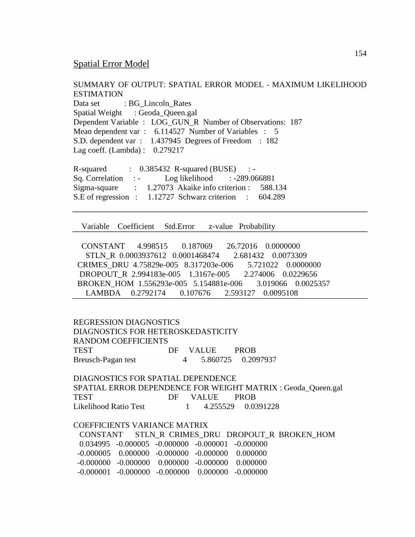
154
Spatial Error Model
SUMMARY OF OUTPUT: SPATIAL ERROR MODEL - MAXIMUM LIKELIHOOD
ESTIMATION
Data set : BG_Lincoln_Rates
Spatial Weight : Geoda_Queen.gal
Dependent Variable : LOG_GUN_R Number of Observations: 187
Mean dependent var : 6.114527 Number of Variables : 5
S.D. dependent var : 1.437945 Degrees of Freedom : 182
Lag coeff. (Lambda) : 0.279217
R-squared : 0.385432 R-squared (BUSE) : -
Sq. Correlation : - Log likelihood : -289.066881
Sigma-square : 1.27073 Akaike info criterion : 588.134
S.E of regression : 1.12727 Schwarz criterion : 604.289
Variable Coefficient Std.Error z-value Probability
CONSTANT 4.998515 0.187069 26.72016 0.0000000
STLN_R 0.0003937612 0.0001468474 2.681432 0.0073309
CRIMES_DRU 4.75829e-005 8.317203e-006 5.721022 0.0000000
DROPOUT_R 2.994183e-005 1.3167e-005 2.274006 0.0229656
BROKEN_HOM 1.556293e-005 5.154881e-006 3.019066 0.0025357
LAMBDA 0.2792174 0.107676 2.593127 0.0095108
REGRESSION DIAGNOSTICS
DIAGNOSTICS FOR HETEROSKEDASTICITY
RANDOM COEFFICIENTS
TEST DF VALUE PROB
Breusch-Pagan test 4 5.860725 0.2097937
DIAGNOSTICS FOR SPATIAL DEPENDENCE
SPATIAL ERROR DEPENDENCE FOR WEIGHT MATRIX : Geoda_Queen.gal
TEST DF VALUE PROB
Likelihood Ratio Test 1 4.255529 0.0391228
COEFFICIENTS VARIANCE MATRIX
CONSTANT STLN_R CRIMES_DRU DROPOUT_R BROKEN_HOM
0.034995 -0.000005 -0.000000 -0.000001 -0.000000
-0.000005 0.000000 -0.000000 -0.000000 0.000000
-0.000000 -0.000000 0.000000 -0.000000 0.000000
-0.000001 -0.000000 -0.000000 0.000000 -0.000000

155
-0.000000 0.000000 0.000000 -0.000000 0.000000
0.000000 0.000000 0.000000 0.000000 0.000000
LAMBDA
0.000000
0.000000
0.000000
0.000000
0.000000
0.011594
OBS LOG_GUN_R PREDICTED RESIDUAL PRED ERROR
1 6.4249 6.00456 0.31716 0.42034
2 6.9458 5.60663 1.20275 1.33913
3 7.5411 7.58636 -0.16986 -0.04529
4 5.0774 5.07239 0.55429 0.00505
5 4.7799 5.24933 -0.33886 -0.46944
6 7.4109 6.76069 0.45831 0.65020
7 6.7738 7.02867 -0.49391 -0.25488
8 6.1215 5.53390 0.40028 0.58759
9 6.4112 6.28703 0.06890 0.12413
10 7.8356 6.72082 0.94031 1.11480
11 4.8964 5.41646 -0.49111 -0.52010
12 6.5492 5.55713 1.12857 0.99206
13 6.9096 6.19678 0.55445 0.71280
14 6.4086 5.55459 0.73238 0.85404
15 6.9188 5.96679 0.75855 0.95201
16 6.3966 5.57584 0.67543 0.82076
17 5.9037 5.85808 -0.02618 0.04567
18 7.0618 6.58920 0.35138 0.47256
19 6.2944 5.81923 0.30954 0.47519
20 5.0216 5.37507 -0.24878 -0.35343
21 6.0587 7.60087 -1.49247 -1.54214
22 7.3599 7.05125 0.06829 0.30865
23 6.8632 6.06027 0.71134 0.80292
24 7.2077 7.06473 0.06938 0.14294
25 5.9558 5.27483 0.94175 0.68097
26 7.8379 7.82659 -0.03683 0.01127
27 7.591 7.49538 -0.06294 0.09560
28 7.903 6.44880 1.31043 1.45420
29 7.9171 6.62596 1.20064 1.29116
30 0 5.03804 -4.77284 -5.03804
31 5.1565 5.35219 0.13887 -0.19565
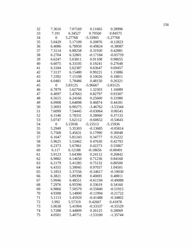
156
32 7.3616 7.07169 0.11665 0.28996
33 7.191 6.34527 0.70560 0.84575
34 0 5.27768 -5.33905 -5.27768
35 5.0429 5.17109 0.20876 -0.12823
36 6.4086 6.78950 -0.49824 -0.38087
37 7.3114 6.88258 0.31930 0.42881
38 6.2704 6.32801 -0.17184 -0.05759
39 6.6247 5.63811 0.91108 0.98655
40 6.6075 6.33105 0.19241 0.27648
41 6.3184 5.62387 0.63647 0.69457
42 7.3137 6.15480 0.99221 1.15886
43 7.3392 7.15108 0.10026 0.18811
44 6.0481 5.78486 0.48150 0.26321
45 0 5.83125 -5.96667 -5.83125
46 6.7879 5.62704 1.32303 1.16089
47 6.4097 5.47663 0.82797 0.93307
48 6.5615 6.24166 0.25600 0.31980
49 6.0908 5.64898 0.46874 0.44181
50 3.3693 6.90275 -3.46762 -3.53344
51 7.6099 7.54445 -0.03064 0.06541
52 6.1546 5.78331 0.28060 0.37133
53 5.0747 5.62112 -0.60652 -0.54641
54 0 5.15936 -5.15513 -5.15936
55 5.2949 5.35303 -0.13685 -0.05814
56 5.7568 5.45631 0.17990 0.30048
57 6.1647 5.81243 0.34777 0.35222
58 5.9625 5.53462 0.47630 0.42793
59 6.2373 5.67861 0.42273 0.55867
60 6.117 6.12188 -0.18656 -0.00491
61 5.9123 5.64386 0.24112 0.26842
62 6.9882 6.14650 0.71236 0.84168
63 6.2179 5.41285 0.75132 0.80500
64 6.4355 5.39045 0.97037 1.04501
65 5.1853 5.37556 -0.24617 -0.19030
66 6.3821 5.89398 0.40691 0.48811
67 5.9946 6.48551 -0.61194 -0.49088
68 7.2976 6.95596 0.33619 0.34160
69 6.9866 7.50579 -0.55840 -0.51915
70 4.9308 5.14800 -0.11994 -0.21722
71 5.1113 5.45929 -0.41488 -0.34802
72 5.992 5.57319 0.42667 0.41878
73 5.0638 5.41904 -0.33337 -0.35529
74 5.7288 5.44809 0.26125 0.28069
75 4.0501 5.40751 -1.53100 -1.35744

157
76 5.1511 5.28720 -0.05302 -0.13608
77 7.483 6.83227 0.66392 0.65071
78 5.7619 5.79093 -0.12431 -0.02901
79 6.9526 6.37098 0.43045 0.58162
80 5.7913 5.29071 0.84487 0.50060
81 7.7025 6.72648 0.94356 0.97599
82 6.6609 6.15132 0.50762 0.50956
83 6.977 5.50338 1.40188 1.47359
84 5.9876 5.98009 -0.05228 0.00751
85 6.487 5.62547 0.93543 0.86151
86 7.481 9.93093 -2.38589 -2.44991
87 7.0955 7.37890 -0.24654 -0.28338
88 4.4356 5.15647 -0.65115 -0.72087
89 4.8064 5.22537 -0.49571 -0.41901
90 5.3863 5.70810 -0.43596 -0.32181
91 6.9426 6.16469 0.66519 0.77793
92 5.7929 5.36101 0.37321 0.43193
93 4.8665 5.29532 -0.55631 -0.42882
94 4.4422 5.36417 -0.87944 -0.92196
95 6.3753 5.84199 0.59900 0.53332
96 4.4606 5.56888 -1.21264 -1.10824
97 6.9088 6.02922 0.81254 0.87954
98 6.1071 6.16651 -0.15529 -0.05942
99 7.7678 6.78367 0.84757 0.98411
100 6.7078 6.35327 0.24563 0.35452
101 5.2758 5.88307 -0.56266 -0.60724
102 5.7247 5.52718 0.15061 0.19753
103 5.2906 5.53874 -0.30938 -0.24809
104 8.2155 7.42680 0.75485 0.78871
105 7.0319 6.00132 1.46310 1.03062
106 5.7252 6.22769 -0.59780 -0.50247
107 4.8203 5.27960 -0.07429 -0.45931
108 5.3677 6.38766 -1.04226 -1.01995
109 5.7675 5.83011 -0.11146 -0.06264
110 6.4294 6.58498 -0.37353 -0.15556
111 6.4636 5.75759 0.57257 0.70597
112 6.4256 5.73064 0.51540 0.69494
113 7.8025 5.95121 1.71133 1.85126
114 7.8627 6.37828 1.40173 1.48437
115 7.2805 5.58055 1.52816 1.69993
116 7.2562 5.98876 1.10776 1.26749
117 7.1435 7.32837 -0.46550 -0.18489
118 8.2594 7.73340 0.40672 0.52597
119 7.2774 7.07883 0.06381 0.19862

158
120 7.222 6.93916 0.10393 0.28279
121 7.6477 7.24527 0.33013 0.40238
122 8.5788 8.70222 0.22615 -0.12347
123 8.7305 9.90340 -1.04966 -1.17293
124 7.1941 7.66118 -0.26718 -0.46704
125 7.238 6.38698 0.68071 0.85107
126 7.9657 8.63397 -0.64227 -0.66822
127 6.8361 6.42615 0.42651 0.40994
128 7.5407 6.65953 0.75874 0.88112
129 7.262 7.10725 -0.02761 0.15472
130 6.9527 6.77889 0.11087 0.17377
131 8.1363 6.64636 1.38551 1.48996
132 6.8801 6.61937 0.08845 0.26074
133 6.471 6.39571 -0.04631 0.07534
134 6.2987 5.70112 0.54367 0.59762
135 6.0728 5.38580 0.54907 0.68702
136 6.9866 6.12535 0.84748 0.86129
137 7.439 6.46253 0.73214 0.97644
138 6.7764 5.92037 0.72116 0.85604
139 7.8229 6.69676 0.88161 1.12613
140 4.5975 5.75690 -0.90279 -1.15944
141 0 5.24740 -5.08391 -5.24740
142 4.7808 5.28906 -0.30438 -0.50823
143 5.6786 5.76762 0.22542 -0.08900
144 6.2254 6.32411 -0.05264 -0.09873
145 5.8201 6.05123 -0.22189 -0.23108
146 4.5984 5.69323 -1.03571 -1.09480
147 6.4208 5.79380 0.73666 0.62701
148 5.6566 5.65032 -0.00983 0.00627
149 6.3657 5.65730 0.75828 0.70840
150 4.9485 6.19584 -1.31260 -1.24737
151 6.4086 6.03799 0.40276 0.37063
152 5.6721 5.55361 0.09874 0.11849
153 5.6575 6.07241 -0.47050 -0.41487
154 5.9677 5.81547 0.05500 0.15224
155 6.0653 5.28474 0.71402 0.78055
156 4.4803 5.31899 -0.83585 -0.83871
157 5.6707 5.88475 -0.06724 -0.21409
158 5.9387 5.87585 0.12159 0.06282
159 4.3489 5.56124 -1.34126 -1.21232
160 6.8955 6.16551 0.87902 0.73002
161 7.3724 5.90247 1.43581 1.46994
162 7.1867 6.10197 1.00762 1.08470
163 7.9099 6.98069 0.79335 0.92917

159
164 6.0282 6.05643 0.01460 -0.02826
165 5.8425 5.47975 0.14632 0.36276
166 5.295 6.06745 -0.95458 -0.77246
167 6.9482 6.75951 -0.00885 0.18873
168 7.1317 6.30517 0.67166 0.82653
169 6.0668 6.04152 -0.02263 0.02526
170 5.0138 5.71769 -0.71888 -0.70388
171 5.4587 5.35066 0.29154 0.10800
172 5.2227 5.21659 0.08659 0.00610
173 7.0793 6.14604 0.86284 0.93325
174 5.4852 5.54378 -0.11817 -0.05859
175 5.3153 5.98554 -0.61077 -0.67022
176 5.737 5.46845 0.27080 0.26851
177 3.9076 5.34221 -1.30191 -1.43458
178 4.9889 5.29590 -0.21055 -0.30702
179 5.0819 5.41143 -0.14376 -0.32950
180 4.5621 5.24636 -0.61254 -0.68424
181 4.7261 5.21403 -0.41193 -0.48791
182 5.4816 5.30674 0.27402 0.17487
183 4.7516 5.71147 -0.87607 -0.95989
184 5.4283 5.16740 0.36540 0.26088
185 5.025 5.55031 -0.49294 -0.52530
186 6.9104 6.19657 0.62000 0.71385
187 6.0196 5.89571 0.03769 0.12385
========================= END OF
REPORT==============================

160

161
Violent Crime Geoda Results
Classic OLS
SUMMARY OF OUTPUT: ORDINARY LEAST SQUARES ESTIMATION
Data set : BG_Lincoln
Dependent Variable : LOG_VIOLEN Number of Observations: 187
Mean dependent var : 5.18569 Number of Variables : 4
S.D. dependent var : 1.01582 Degrees of Freedom : 183
R-squared : 0.528459 F-statistic : 68.3631
Adjusted R-squared : 0.520729 Prob(F-statistic) :1.06063e-029
Sum squared residual: 90.99 Log likelihood : -197.988
Sigma-square : 0.497213 Akaike info criterion : 403.976
S.E. of regression : 0.705133 Schwarz criterion : 416.9
Sigma-square ML : 0.486577
S.E of regression ML: 0.697551
Variable Coefficient Std.Error t-Statistic Probability
CONSTANT 4.18078 0.09632361 43.40348 0.0000000
RCVD 0.02750526 0.005712729 4.814731 0.0000031
CRIMES_DRU 0.00563155 0.0007275727 7.74019 0.0000000
BROKEN_HOM 1.493377 0.2963614 5.039039 0.0000011
REGRESSION DIAGNOSTICS
MULTICOLLINEARITY CONDITION NUMBER 4.092541
TEST ON NORMALITY OF ERRORS
TEST DF VALUE PROB
Jarque-Bera 2 581.2829 0.0000000
DIAGNOSTICS FOR HETEROSKEDASTICITY
RANDOM COEFFICIENTS
TEST DF VALUE PROB
Breusch-Pagan test 3 9.108504 0.0278825
Koenker-Bassett test 3 1.874033 0.5989586
SPECIFICATION ROBUST TEST
TEST DF VALUE PROB
White 9 35.65997 0.0000455

162
DIAGNOSTICS FOR SPATIAL DEPENDENCE
FOR WEIGHT MATRIX : Geoda_Queen.gal
(row-standardized weights)
TEST MI/DF VALUE PROB
Moran's I (error) 0.187569 4.6538004 0.0000033
Lagrange Multiplier (lag) 1 12.5984247 0.0003861
Robust LM (lag) 1 0.4397971 0.5072204
Lagrange Multiplier (error) 1 18.5481601 0.0000166
Robust LM (error) 1 6.3895325 0.0114795
Lagrange Multiplier (SARMA) 2 18.9879572 0.0000753
COEFFICIENTS VARIANCE MATRIX
CONSTANT RCVD CRIMES_DRU BROKEN_HOM
0.009278 -0.000138 -0.000011 -0.018380
-0.000138 0.000033 -0.000002 -0.000153
-0.000011 -0.000002 0.000001 -0.000037
-0.018380 -0.000153 -0.000037 0.087830
OBS LOG_VIOLEN PREDICTED RESIDUAL
1 5.34711 5.01036 0.33675
2 5.34233 5.07945 0.26289
3 6.21261 6.49310 -0.28049
4 4.35671 4.27848 0.07823
5 4.71850 4.61378 0.10472
6 5.86647 5.53158 0.33489
7 6.02587 6.01232 0.01354
8 4.64439 4.60890 0.03549
9 6.12468 5.46743 0.65725
10 6.39859 6.09338 0.30521
11 3.71357 4.38966 -0.67609
12 4.12713 4.59776 -0.47062
13 4.89035 5.20715 -0.31680
14 4.70048 4.64031 0.06017
15 4.67283 4.84792 -0.17509
16 5.35659 4.94819 0.40839
17 5.79606 4.78827 1.00778
18 6.24998 5.77096 0.47902
19 5.80814 5.12177 0.68638
20 4.82028 4.75011 0.07017
21 4.48864 4.61983 -0.13119
22 4.82028 5.28869 -0.46841
23 5.48894 5.02858 0.46036
24 6.49072 5.99773 0.49299

163
25 4.02535 4.39152 -0.36616
26 6.10702 6.38934 -0.28231
27 6.29157 5.51653 0.77504
28 6.67077 6.62114 0.04963
29 5.96358 5.39012 0.57346
30 2.30259 4.35471 -2.05212
31 3.68888 4.65357 -0.96469
32 6.34036 5.63490 0.70546
33 6.17794 5.90887 0.26907
34 3.36730 4.56431 -1.19702
35 5.27300 4.69476 0.57824
36 5.89440 6.21900 -0.32460
37 5.18178 5.26750 -0.08572
38 5.12396 5.27326 -0.14930
39 4.96284 4.76749 0.19536
40 4.86753 5.20513 -0.33760
41 4.97673 5.11121 -0.13448
42 6.23441 5.69513 0.53928
43 4.46591 4.54161 -0.07570
44 5.80212 4.91474 0.88738
45 0.00000 4.19204 -4.19204
46 4.67283 4.42779 0.24504
47 5.74620 5.02056 0.72565
48 6.11368 6.35829 -0.24461
49 5.35659 5.14433 0.21225
50 2.94444 5.82621 -2.88177
51 6.22654 6.13893 0.08760
52 6.25767 5.28993 0.96774
53 5.47646 5.15187 0.32460
54 2.39790 4.34668 -1.94878
55 4.18965 4.43709 -0.24743
56 5.40268 5.05114 0.35154
57 6.38012 5.36177 1.01835
58 4.51086 4.49166 0.01920
59 5.53733 5.01899 0.51834
60 6.33859 5.04304 1.29556
61 4.99043 5.00820 -0.01776
62 5.83773 5.02851 0.80922
63 5.40268 4.86229 0.54039
64 5.22575 4.77837 0.44737
65 4.14313 4.43631 -0.29318
66 5.11799 5.00729 0.11070
67 5.16479 5.43876 -0.27398
68 6.31897 5.84371 0.47526
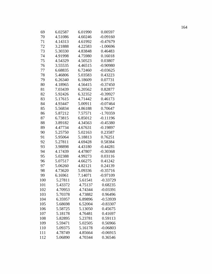
164
69 6.02587 6.01990 0.00597
70 4.51086 4.60246 -0.09160
71 4.14313 4.61992 -0.47679
72 3.21888 4.22583 -1.00696
73 5.30330 4.83848 0.46483
74 4.91998 4.75980 0.16018
75 4.54329 4.50523 0.03807
76 3.55535 4.46515 -0.90980
77 6.68835 6.72460 -0.03625
78 5.46806 5.03583 0.43223
79 6.26340 6.18609 0.07731
80 4.18965 4.56415 -0.37450
81 7.03439 6.20562 0.82877
82 5.92426 6.32352 -0.39927
83 5.17615 4.71442 0.46173
84 4.93447 5.00911 -0.07464
85 5.56834 4.86188 0.70647
86 5.87212 7.57571 -1.70359
87 6.73815 6.85012 -0.11196
88 3.89182 4.34563 -0.45380
89 4.47734 4.67631 -0.19897
90 5.25750 5.02163 0.23587
91 5.95064 5.18813 0.76251
92 5.27811 4.69428 0.58384
93 3.98898 4.43180 -0.44281
94 4.17439 4.47807 -0.30368
95 5.02388 4.99273 0.03116
96 5.07517 4.66275 0.41242
97 5.06260 4.82121 0.24139
98 4.73620 5.09336 -0.35716
99 6.16961 7.14071 -0.97109
100 5.27811 5.61541 -0.33729
101 5.43372 4.75137 0.68235
102 4.70953 4.74344 -0.03391
103 5.70378 4.73882 0.96496
104 6.35957 6.89896 -0.53939
105 5.68698 6.52004 -0.83307
106 5.58725 5.13050 0.45675
107 5.18178 4.76481 0.41697
108 5.82895 5.23781 0.59113
109 5.59471 5.02505 0.56966
110 5.09375 5.16178 -0.06803
111 4.78749 4.85664 -0.06915
112 5.06890 4.70344 0.36546
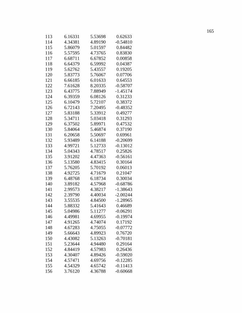
165
113 6.16331 5.53698 0.62633
114 4.34381 4.89190 -0.54810
115 5.86079 5.01597 0.84482
116 5.57595 4.73765 0.83830
117 6.68711 6.67852 0.00858
118 6.64379 6.59992 0.04387
119 5.62762 5.43557 0.19205
120 5.83773 5.76067 0.07706
121 6.66185 6.01633 0.64553
122 7.61628 8.20335 -0.58707
123 6.43775 7.88949 -1.45174
124 6.39359 6.08126 0.31233
125 6.10479 5.72107 0.38372
126 6.72143 7.20495 -0.48352
127 5.83188 5.33912 0.49277
128 5.34711 5.03418 0.31293
129 6.37502 5.89971 0.47532
130 5.84064 5.46874 0.37190
131 6.20658 5.50697 0.69961
132 5.93489 6.14188 -0.20699
133 4.99721 5.12733 -0.13012
134 5.04343 4.78517 0.25826
135 3.91202 4.47363 -0.56161
136 5.13580 4.83415 0.30164
137 5.76205 5.70192 0.06013
138 4.92725 4.71679 0.21047
139 6.48768 6.18734 0.30034
140 3.89182 4.57968 -0.68786
141 2.99573 4.38217 -1.38643
142 2.39790 4.40034 -2.00244
143 3.55535 4.84500 -1.28965
144 5.88332 5.41643 0.46689
145 5.04986 5.11277 -0.06291
146 4.49981 4.69955 -0.19974
147 4.91265 4.74074 0.17192
148 4.67283 4.75055 -0.07772
149 5.66643 4.89923 0.76720
150 4.43082 5.13263 -0.70181
151 5.23644 4.94480 0.29164
152 4.84419 4.57983 0.26436
153 4.30407 4.89426 -0.59020
154 4.57471 4.69756 -0.12285
155 4.54329 4.65742 -0.11413
156 3.76120 4.36788 -0.60668

166
157 4.46591 4.98510 -0.51919
158 4.60517 4.99045 -0.38528
159 4.34381 4.75314 -0.40933
160 4.26268 5.04759 -0.78491
161 5.52146 5.22256 0.29890
162 7.18690 7.09745 0.08945
163 5.96615 5.74156 0.22459
164 5.83188 4.95410 0.87778
165 5.52146 4.33781 1.18365
166 6.08450 5.14996 0.93454
167 6.16961 5.59970 0.56991
168 6.00389 5.59654 0.40734
169 5.47227 5.28842 0.18385
170 4.45435 4.88756 -0.43321
171 4.46591 4.47288 -0.00698
172 4.77068 4.46504 0.30564
173 5.94017 5.56274 0.37743
174 5.12396 4.68705 0.43691
175 5.30827 5.04915 0.25912
176 4.53260 4.60748 -0.07488
177 4.14313 4.56136 -0.41822
178 4.82831 4.58459 0.24373
179 4.53260 4.62221 -0.08961
180 4.52179 4.93364 -0.41185
181 5.69036 4.39702 1.29334
182 3.66356 4.34368 -0.68012
183 4.57471 4.99306 -0.41835
184 3.46574 4.28019 -0.81445
185 4.79579 4.59709 0.19870
186 5.14749 4.76642 0.38107
187 5.22036 5.27065 -0.05029
========================= END OF REPORT
==============================

167

168
Spatial Lag Model
SUMMARY OF OUTPUT: SPATIAL LAG MODEL - MAXIMUM LIKELIHOOD
ESTIMATION
Data set : BG_Lincoln
Spatial Weight : Geoda_Queen.gal
Dependent Variable : LOG_VIOLEN Number of Observations: 187
Mean dependent var : 5.18569 Number of Variables : 5
S.D. dependent var : 1.01582 Degrees of Freedom : 182
Lag coeff. (Rho) : 0.271346
R-squared : 0.562160 Log likelihood : -192.301
Sq. Correlation : - Akaike info criterion : 394.602
Sigma-square : 0.451802 Schwarz criterion : 410.758
S.E of regression : 0.672162
Variable Coefficient Std.Error z-value Probability
W_LOG_VIOLEN 0.2713455 0.07829576 3.465648 0.0005290
CONSTANT 2.91341 0.3749824 7.769459 0.0000000
RCVD 0.02489149 0.005494839 4.529976 0.0000059
CRIMES_DRU 0.004677244 0.0007691415 6.081123 0.0000000
BROKEN_HOM 1.234482 0.2886049 4.277411 0.0000189
REGRESSION DIAGNOSTICS
DIAGNOSTICS FOR HETEROSKEDASTICITY
RANDOM COEFFICIENTS
TEST DF VALUE PROB
Breusch-Pagan test 3 14.06316 0.0028204
DIAGNOSTICS FOR SPATIAL DEPENDENCE
SPATIAL LAG DEPENDENCE FOR WEIGHT MATRIX : Geoda_Queen.gal
TEST DF VALUE PROB
Likelihood Ratio Test 1 11.37385 0.0007449
COEFFICIENTS VARIANCE MATRIX
CONSTANT RCVD CRIMES_DRU BROKEN_HOM W_LOG_VIOLEN
0.140612 0.000142 0.000111 0.004759 -0.028466
0.000142 0.000030 -0.000001 -0.000095 -0.000057
0.000111 -0.000001 0.000001 -0.000014 -0.000026
0.004759 -0.000095 -0.000014 0.083293 -0.004622
-0.028466 -0.000057 -0.000026 -0.004622 0.006130

169
OBS LOG_VIOLEN PREDICTED RESIDUAL PRED ERROR
1 5.3471 5.09591 0.04653 0.25120
2 5.3423 5.15086 0.11331 0.19147
3 6.2126 6.46261 -0.29802 -0.25000
4 4.3567 4.20781 0.30174 0.14890
5 4.7185 4.50763 0.31438 0.21087
6 5.8665 5.50231 0.37864 0.36416
7 6.0259 5.94493 0.00863 0.08094
8 4.6444 4.58633 0.02142 0.05806
9 6.1247 5.45030 0.62075 0.67439
10 6.3986 6.27193 0.13075 0.12667
11 3.7136 4.31561 -0.59102 -0.60204
12 4.1271 4.49485 -0.31998 -0.36771
13 4.8903 5.20461 -0.39109 -0.31427
14 4.7005 4.68851 -0.12471 0.01198
15 4.6728 4.84449 -0.21143 -0.17167
16 5.3566 4.87833 0.42826 0.47826
17 5.7961 4.79276 0.92230 1.00329
18 6.25 5.70883 0.48965 0.54115
19 5.8081 5.13107 0.61039 0.67707
20 4.8203 4.64012 0.20184 0.18016
21 4.4886 4.51542 -0.03463 -0.02678
22 4.8203 5.46759 -0.73787 -0.64731
23 5.4889 5.17351 0.25294 0.31543
24 6.4907 6.07619 0.48612 0.41454
25 4.0254 4.35218 -0.28125 -0.32683
26 6.107 6.32215 -0.28872 -0.21513
27 6.2916 5.72507 0.65118 0.56650
28 6.6708 6.69530 0.02264 -0.02454
29 5.9636 5.54247 0.32394 0.42111
30 2.3026 5.00209 -2.29622 -2.69950
31 3.6889 4.52835 -0.83904 -0.83947
32 6.3404 5.76232 0.57179 0.57804
33 6.1779 5.92797 0.26832 0.24997
34 3.3673 4.43202 -0.99667 -1.06473
35 5.273 4.56993 0.78149 0.70307
36 5.8944 6.21386 -0.33986 -0.31945
37 5.1818 5.32469 -0.16608 -0.14291
38 5.124 5.40785 -0.25699 -0.28389
39 4.9628 5.06896 -0.06609 -0.10611
40 4.8675 5.16453 -0.43041 -0.29700
41 4.9767 5.05531 -0.11463 -0.07857

170
42 6.2344 5.73354 0.46975 0.50087
43 4.4659 4.63074 -0.34964 -0.16483
44 5.8021 4.79050 1.22329 1.01162
45 0 4.20701 -4.22546 -4.20701
46 4.6728 4.39799 0.38795 0.27484
47 5.7462 5.24948 0.45942 0.49672
48 6.1137 6.35931 -0.30750 -0.24563
49 5.3566 5.26529 0.03975 0.09130
50 2.9444 6.05634 -2.95451 -3.11190
51 6.2265 6.18860 0.15309 0.03794
52 6.2577 5.34940 0.83830 0.90826
53 5.4765 5.19687 0.19394 0.27959
54 2.3979 4.26291 -1.94284 -1.86502
55 4.1897 4.44884 -0.33112 -0.25918
56 5.4027 4.96644 0.41999 0.43624
57 6.3801 5.35333 0.97589 1.02680
58 4.5109 4.68357 -0.30753 -0.17271
59 5.5373 5.03942 0.35777 0.49791
60 6.3386 5.05536 1.22530 1.28323
61 4.9904 4.94249 0.02545 0.04795
62 5.8377 5.04046 0.70379 0.79727
63 5.4027 4.83360 0.50676 0.56908
64 5.2257 4.72229 0.40830 0.50345
65 4.1431 4.37323 -0.23294 -0.23010
66 5.118 4.98546 0.05616 0.13254
67 5.1648 5.31583 -0.20642 -0.15105
68 6.319 6.01973 0.32741 0.29924
69 6.0259 6.17153 -0.16225 -0.14567
70 4.5109 4.55891 -0.10507 -0.04805
71 4.1431 4.61942 -0.62403 -0.47629
72 3.2189 4.24530 -1.13825 -1.02642
73 5.3033 4.74343 0.46997 0.55987
74 4.92 4.69512 0.12682 0.22486
75 4.5433 4.71787 -0.27999 -0.17458
76 3.5553 4.41378 -0.85981 -0.85843
77 6.6884 6.84248 -0.03736 -0.15412
78 5.4681 4.94993 0.47767 0.51813
79 6.2634 6.20972 -0.05119 0.05368
80 4.1897 4.47626 -0.19503 -0.28660
81 7.0344 6.26604 0.80480 0.76835
82 5.9243 6.23852 -0.37939 -0.31426
83 5.1761 4.74868 0.39168 0.42747
84 4.9345 5.02387 -0.19695 -0.08940
85 5.5683 4.78614 0.73244 0.78221

171
86 5.8721 7.63057 -1.71639 -1.75845
87 6.7382 6.85249 -0.09295 -0.11434
88 3.8918 4.29108 -0.36522 -0.39926
89 4.4773 4.67940 -0.27366 -0.20206
90 5.2575 4.95462 0.21001 0.30287
91 5.9506 5.06756 0.71811 0.88308
92 5.2781 4.66739 0.50925 0.61072
93 3.989 4.36911 -0.36890 -0.38012
94 4.1744 4.40405 -0.26592 -0.22966
95 5.0239 4.84970 0.16380 0.17418
96 5.0752 4.62306 0.43294 0.45211
97 5.0626 4.78855 0.22445 0.27404
98 4.7362 5.01368 -0.31072 -0.27748
99 6.1696 7.02565 -0.86870 -0.85603
100 5.2781 5.48487 -0.25673 -0.20676
101 5.4337 4.64393 0.76319 0.78979
102 4.7095 4.69818 -0.06345 0.01135
103 5.7038 4.71262 0.92305 0.99116
104 6.3596 6.96798 -0.50179 -0.60841
105 5.687 6.62047 -0.65956 -0.93349
106 5.5872 5.18203 0.35211 0.40522
107 5.1818 4.60154 0.81152 0.58024
108 5.8289 5.10182 0.62714 0.72713
109 5.5947 5.05882 0.53781 0.53589
110 5.0938 5.10688 -0.05172 -0.01313
111 4.7875 5.00353 -0.20017 -0.21604
112 5.0689 4.81151 0.29777 0.25740
113 6.1633 5.62730 0.55683 0.53601
114 4.3438 4.87501 -0.59870 -0.53120
115 5.8608 5.21126 0.58931 0.64952
116 5.5759 4.99554 0.51370 0.58041
117 6.6871 6.57565 0.00308 0.11146
118 6.6438 6.50768 0.07968 0.13611
119 5.6276 5.69564 -0.11718 -0.06802
120 5.8377 5.70459 0.08368 0.13314
121 6.6619 6.30065 0.45962 0.36121
122 7.6163 8.08749 -0.19822 -0.47120
123 6.4378 7.86602 -1.24590 -1.42827
124 6.3936 6.34715 0.16657 0.04644
125 6.1048 5.75783 0.28668 0.34696
126 6.7214 7.21583 -0.44505 -0.49441
127 5.8319 5.53379 0.29395 0.29809
128 5.3471 5.19619 0.09103 0.15091
129 6.375 5.84252 0.49367 0.53250

172
130 5.8406 5.57543 0.25001 0.26521
131 6.2066 5.70640 0.47228 0.50018
132 5.9349 6.20759 -0.32650 -0.27269
133 4.9972 5.05606 -0.09321 -0.05885
134 5.0434 4.72817 0.40002 0.31525
135 3.912 4.52619 -0.52736 -0.61417
136 5.1358 4.86096 0.38597 0.27484
137 5.7621 5.58683 0.12902 0.17522
138 4.9273 4.79094 0.09800 0.13631
139 6.4877 6.08616 0.35324 0.40152
140 3.8918 4.50968 -0.47773 -0.61786
141 2.9957 4.30561 -0.97484 -1.30988
142 2.3979 4.35491 -1.81093 -1.95701
143 3.5553 4.68461 -0.90221 -1.12926
144 5.8833 5.22687 0.64734 0.65645
145 5.0499 5.01669 -0.04083 0.03317
146 4.4998 4.61209 -0.04852 -0.11228
147 4.9127 4.71805 0.14602 0.19460
148 4.6728 4.75102 -0.12460 -0.07819
149 5.6664 4.78124 0.91497 0.88518
150 4.4308 4.99820 -0.66648 -0.56738
151 5.2364 4.82089 0.36721 0.41555
152 4.8442 4.50230 0.39251 0.34189
153 4.3041 4.77072 -0.45383 -0.46666
154 4.5747 4.64115 -0.15340 -0.06644
155 4.5433 4.60454 -0.09587 -0.06125
156 3.7612 4.33256 -0.48997 -0.57136
157 4.4659 4.84167 -0.17736 -0.37576
158 4.6052 4.85957 -0.07284 -0.25440
159 4.3438 4.75450 -0.33347 -0.41069
160 4.2627 4.90127 -0.47895 -0.63859
161 5.5215 5.18637 0.32660 0.33509
162 7.1869 6.87557 0.23495 0.31133
163 5.9661 5.74233 0.09307 0.22381
164 5.8319 4.93009 0.76879 0.90180
165 5.5215 4.59294 0.81607 0.92853
166 6.0845 5.26067 0.70525 0.82383
167 6.1696 5.54288 0.52298 0.62674
168 6.0039 5.52038 0.33729 0.48351
169 5.4723 5.09038 0.26865 0.38189
170 4.4543 4.76835 -0.39142 -0.31401
171 4.4659 4.41591 0.11565 0.05000
172 4.7707 4.48230 0.27501 0.28839
173 5.9402 5.31071 0.65281 0.62946

173
174 5.124 4.62466 0.48330 0.49930
175 5.3083 4.89319 0.39948 0.41508
176 4.5326 4.56271 -0.12638 -0.03011
177 4.1431 4.47866 -0.23483 -0.33552
178 4.8283 4.53077 0.28009 0.29754
179 4.5326 4.52749 0.06023 0.00511
180 4.5218 4.79510 -0.27665 -0.27331
181 5.6904 4.32430 1.42073 1.36606
182 3.6636 4.29220 -0.69732 -0.62864
183 4.5747 4.83461 -0.19191 -0.25990
184 3.4657 4.27705 -0.76735 -0.81131
185 4.7958 4.50037 0.37338 0.29542
186 5.1475 4.69791 0.39067 0.44959
187 5.2204 5.04546 0.21440 0.17490
========================= END OF
REPORT==============================

174

175
Spatial Error Model
SUMMARY OF OUTPUT: SPATIAL ERROR MODEL - MAXIMUM LIKELIHOOD
ESTIMATION
Data set : BG_Lincoln
Spatial Weight : Geoda_Queen.gal
Dependent Variable : LOG_VIOLEN Number of Observations: 187
Mean dependent var : 5.185692 Number of Variables : 4
S.D. dependent var : 1.015819 Degrees of Freedom : 183
Lag coeff. (Lambda) : 0.435168
R-squared : 0.583887 R-squared (BUSE) : -
Sq. Correlation : - Log likelihood : -189.714089
Sigma-square : 0.429382 Akaike info criterion : 387.428
S.E of regression : 0.655273 Schwarz criterion : 400.353
Variable Coefficient Std.Error z-value Probability
CONSTANT 4.231727 0.121443 34.84536 0.0000000
RCVD 0.02489559 0.005586281 4.456559 0.0000083
CRIMES_DRU 0.005930874 0.0008010239 7.404117 0.0000000
BROKEN_HOM 1.250649 0.2869593 4.35828 0.0000131
LAMBDA 0.4351676 0.09547911 4.557726 0.0000052
REGRESSION DIAGNOSTICS
DIAGNOSTICS FOR HETEROSKEDASTICITY
RANDOM COEFFICIENTS
TEST DF VALUE PROB
Breusch-Pagan test 3 10.55791 0.0143731
DIAGNOSTICS FOR SPATIAL DEPENDENCE
SPATIAL ERROR DEPENDENCE FOR WEIGHT MATRIX : Geoda_Queen.gal
TEST DF VALUE PROB
Likelihood Ratio Test 1 16.54768 0.0000474
COEFFICIENTS VARIANCE MATRIX
CONSTANT RCVD CRIMES_DRU BROKEN_HOM LAMBDA
0.014748 -0.000131 -0.000024 -0.019219 0.000000
-0.000131 0.000031 -0.000002 -0.000112 0.000000
-0.000024 -0.000002 0.000001 -0.000013 0.000000
-0.019219 -0.000112 -0.000013 0.082346 0.000000
0.000000 0.000000 0.000000 0.000000 0.009116

176
OBS LOG_VIOLEN PREDICTED RESIDUAL PRED ERROR
1 5.3471 4.96508 0.00750 0.38203
2 5.3423 5.05920 0.15774 0.28313
3 6.2126 6.37533 -0.28787 -0.16272
4 4.3567 4.32391 0.33228 0.03280
5 4.7185 4.62980 0.29805 0.08869
6 5.8665 5.46384 0.40210 0.40262
7 6.0259 5.88911 -0.01098 0.13675
8 4.6444 4.63885 -0.04753 0.00554
9 6.1247 5.45969 0.56696 0.66499
10 6.3986 6.02259 0.34417 0.37600
11 3.7136 4.42067 -0.64568 -0.70709
12 4.1271 4.59737 -0.34103 -0.47023
13 4.8903 5.15296 -0.39267 -0.26261
14 4.7005 4.67025 -0.18361 0.03023
15 4.6728 4.82524 -0.21361 -0.15241
16 5.3566 4.93967 0.34301 0.41692
17 5.7961 4.85231 0.82094 0.94375
18 6.25 5.68594 0.44947 0.56403
19 5.8081 5.11418 0.56502 0.69397
20 4.8203 4.75491 0.14230 0.06537
21 4.4886 4.64224 -0.11593 -0.15360
22 4.8203 5.21730 -0.57645 -0.39702
23 5.4889 5.00399 0.35593 0.48495
24 6.4907 5.94365 0.60129 0.54708
25 4.0254 4.43250 -0.27937 -0.40715
26 6.107 6.25912 -0.30134 -0.15210
27 6.2916 5.52422 0.85915 0.76735
28 6.6708 6.52980 0.14592 0.14097
29 5.9636 5.39437 0.35806 0.56921
30 2.3026 4.41083 -1.50936 -2.10824
31 3.6889 4.64005 -0.89731 -0.95117
32 6.3404 5.61550 0.63881 0.72486
33 6.1779 5.88525 0.27409 0.29269
34 3.3673 4.56523 -1.04480 -1.19793
35 5.273 4.72451 0.71544 0.54849
36 5.8944 6.21964 -0.40943 -0.32524
37 5.1818 5.27931 -0.16063 -0.09752
38 5.124 5.24154 -0.10918 -0.11757
39 4.9628 4.82340 0.15532 0.13945
40 4.8675 5.16438 -0.50203 -0.29685
41 4.9767 5.07058 -0.13968 -0.09385

177
42 6.2344 5.66963 0.49750 0.56478
43 4.4659 4.57916 -0.42489 -0.11326
44 5.8021 4.89772 1.27547 0.90440
45 0 4.24359 -4.23673 -4.24359
46 4.6728 4.45624 0.43632 0.21659
47 5.7462 5.03516 0.61683 0.71105
48 6.1137 6.22142 -0.26448 -0.10774
49 5.3566 5.13070 0.10395 0.22588
50 2.9444 5.64251 -2.51983 -2.69807
51 6.2265 6.07063 0.25517 0.15590
52 6.2577 5.27491 0.83168 0.98276
53 5.4765 5.12649 0.17871 0.34997
54 2.3979 4.37673 -2.05461 -1.97884
55 4.1897 4.45860 -0.35517 -0.26895
56 5.4027 5.07162 0.31195 0.33106
57 6.3801 5.31466 0.96024 1.06546
58 4.5109 4.51102 -0.23577 -0.00016
59 5.5373 5.02390 0.29606 0.51344
60 6.3386 5.03716 1.21931 1.30144
61 4.9904 4.98909 -0.01645 0.00134
62 5.8377 5.01308 0.67083 0.82466
63 5.4027 4.88716 0.41573 0.51552
64 5.2257 4.79874 0.31215 0.42701
65 4.1431 4.46702 -0.28104 -0.32389
66 5.118 4.95822 0.03860 0.15977
67 5.1648 5.33600 -0.26117 -0.17122
68 6.319 5.83117 0.49482 0.48779
69 6.0259 5.94032 -0.00151 0.08554
70 4.5109 4.63919 -0.17242 -0.12833
71 4.1431 4.63302 -0.72212 -0.48988
72 3.2189 4.27917 -1.24892 -1.06030
73 5.3033 4.82292 0.38281 0.48038
74 4.92 4.74982 0.02539 0.17016
75 4.5433 4.51388 -0.13799 0.02941
76 3.5553 4.48768 -0.88439 -0.93233
77 6.6884 6.63769 0.18972 0.05067
78 5.4681 5.01347 0.40364 0.45459
79 6.2634 6.07695 -0.04362 0.18645
80 4.1897 4.58574 -0.19717 -0.39609
81 7.0344 6.17383 0.85217 0.86056
82 5.9243 6.20525 -0.40414 -0.28100
83 5.1761 4.74009 0.37664 0.43606
84 4.9345 4.98962 -0.23430 -0.05515
85 5.5683 4.89152 0.63542 0.67683

178
86 5.8721 7.76639 -1.85356 -1.89427
87 6.7382 6.78218 -0.07815 -0.04403
88 3.8918 4.37715 -0.37872 -0.48532
89 4.4773 4.69569 -0.31099 -0.21835
90 5.2575 5.00238 0.11953 0.25512
91 5.9506 5.16466 0.53525 0.78598
92 5.2781 4.70743 0.43639 0.57069
93 3.989 4.46446 -0.41893 -0.47547
94 4.1744 4.49892 -0.33647 -0.32453
95 5.0239 4.95494 0.07996 0.06894
96 5.0752 4.65609 0.40033 0.41909
97 5.0626 4.83689 0.16912 0.22571
98 4.7362 5.02529 -0.34361 -0.28909
99 6.1696 7.07483 -0.98170 -0.90522
100 5.2781 5.53066 -0.34546 -0.25255
101 5.4337 4.75524 0.67091 0.67848
102 4.7095 4.73839 -0.12048 -0.02886
103 5.7038 4.73137 0.86744 0.97241
104 6.3596 6.76265 -0.32228 -0.40307
105 5.687 6.38844 -0.37204 -0.70146
106 5.5872 5.16385 0.34059 0.42340
107 5.1818 4.76495 0.82944 0.41683
108 5.8289 5.14520 0.50779 0.68374
109 5.5947 4.99633 0.55875 0.59838
110 5.0938 5.13960 -0.10078 -0.04585
111 4.7875 4.86040 -0.06540 -0.07291
112 5.0689 4.70547 0.41971 0.36344
113 6.1633 5.55680 0.61800 0.60651
114 4.3438 4.87810 -0.64869 -0.53430
115 5.8608 5.08687 0.65204 0.77391
116 5.5759 4.81413 0.61103 0.76182
117 6.6871 6.53862 -0.07131 0.14848
118 6.6438 6.54422 -0.06180 0.09957
119 5.6276 5.42548 0.09033 0.20214
120 5.8377 5.70607 0.03849 0.13166
121 6.6619 6.00489 0.80590 0.65697
122 7.6163 8.33781 -0.37576 -0.72153
123 6.4378 7.82155 -1.16533 -1.38380
124 6.3936 6.06963 0.48318 0.32397
125 6.1048 5.73754 0.19542 0.36725
126 6.7214 7.18582 -0.42954 -0.46439
127 5.8319 5.28413 0.49992 0.54775
128 5.3471 5.05411 0.18039 0.29300
129 6.375 5.90001 0.38988 0.47501

179
130 5.8406 5.42727 0.35350 0.41337
131 6.2066 5.48373 0.67165 0.72285
132 5.9349 6.06962 -0.26129 -0.13472
133 4.9972 5.07674 -0.13544 -0.07952
134 5.0434 4.78525 0.40313 0.25817
135 3.912 4.49520 -0.41789 -0.58318
136 5.1358 4.83452 0.49584 0.30128
137 5.7621 5.57688 0.10596 0.18517
138 4.9273 4.70863 0.16472 0.21862
139 6.4877 6.19465 0.18484 0.29303
140 3.8918 4.58644 -0.42354 -0.69462
141 2.9957 4.41253 -0.83494 -1.41680
142 2.3979 4.43082 -1.77191 -2.03293
143 3.5553 4.83908 -0.89475 -1.28373
144 5.8833 5.47068 0.42561 0.41264
145 5.0499 5.09207 -0.11580 -0.04221
146 4.4998 4.70334 -0.05720 -0.20353
147 4.9127 4.73354 0.15191 0.17911
148 4.6728 4.76727 -0.13543 -0.09444
149 5.6664 4.89179 0.85305 0.77464
150 4.4308 5.05988 -0.75337 -0.62906
151 5.2364 4.92566 0.26977 0.31078
152 4.8442 4.57871 0.38462 0.26548
153 4.3041 4.85354 -0.48189 -0.54947
154 4.5747 4.72047 -0.24229 -0.14575
155 4.5433 4.65972 -0.12871 -0.11642
156 3.7612 4.41765 -0.48773 -0.65645
157 4.4659 4.93656 -0.12205 -0.47066
158 4.6052 4.96541 -0.04277 -0.36024
159 4.3438 4.73129 -0.24092 -0.38749
160 4.2627 4.97603 -0.43310 -0.71335
161 5.5215 5.21203 0.28411 0.30943
162 7.1869 7.09812 -0.10058 0.08878
163 5.9661 5.69937 0.00521 0.26678
164 5.8319 4.90995 0.69662 0.92193
165 5.5215 4.39303 0.90949 1.12843
166 6.0845 5.10248 0.77343 0.98202
167 6.1696 5.50407 0.47154 0.66554
168 6.0039 5.52213 0.22165 0.48176
169 5.4723 5.26403 0.05667 0.20824
170 4.4543 4.84945 -0.48062 -0.39510
171 4.4659 4.50372 0.11527 -0.03781
172 4.7707 4.50217 0.26613 0.26852
173 5.9402 5.48291 0.52902 0.45726

180
174 5.124 4.71345 0.42379 0.41052
175 5.3083 5.02098 0.29814 0.28729
176 4.5326 4.60972 -0.18005 -0.07712
177 4.1431 4.57239 -0.22161 -0.42925
178 4.8283 4.62236 0.22181 0.20595
179 4.5326 4.63728 0.03047 -0.10468
180 4.5218 4.92381 -0.36417 -0.40202
181 5.6904 4.43469 1.38720 1.25567
182 3.6636 4.37422 -0.77816 -0.71066
183 4.5747 4.96921 -0.24703 -0.39449
184 3.4657 4.32421 -0.73014 -0.85847
185 4.7958 4.59317 0.37865 0.20262
186 5.1475 4.75821 0.33936 0.38929
187 5.2204 5.27579 0.04192 -0.05543
========================= END OF
REPORT==============================

181

182
Property Crime Geoda Results
Classic OLS
SUMMARY OF OUTPUT: ORDINARY LEAST SQUARES ESTIMATION
Data set : BG_Lincoln
Dependent Variable : LOG_PROPER Number of Observations: 187
Mean dependent var : 5.98268 Number of Variables : 5
S.D. dependent var : 0.890076 Degrees of Freedom : 182
R-squared : 0.439638 F-statistic : 35.6975
Adjusted R-squared : 0.427323 Prob(F-statistic) :5.29042e-022
Sum squared residual: 83.0165 Log likelihood : -189.413
Sigma-square : 0.456135 Akaike info criterion : 388.826
S.E. of regression : 0.675377 Schwarz criterion : 404.982
Sigma-square ML : 0.443939
S.E of regression ML: 0.666287
Variable Coefficient Std.Error t-Statistic Probability
CONSTANT 5.183483 0.09460903 54.78846 0.0000000
STLN 0.01906406 0.006189306 3.080162 0.0023898
RCVD 0.02346362 0.005585909 4.200501 0.0000417
CRIMES_DRU 0.004237366 0.0006973035 6.076789 0.0000000
BROKEN_HOM 0.900852 0.2845724 3.165634 0.0018144
REGRESSION DIAGNOSTICS
MULTICOLLINEARITY CONDITION NUMBER 4.323249
TEST ON NORMALITY OF ERRORS
TEST DF VALUE PROB
Jarque-Bera 2 3271.469 0.0000000
DIAGNOSTICS FOR HETEROSKEDASTICITY
RANDOM COEFFICIENTS
TEST DF VALUE PROB
Breusch-Pagan test 4 5.056442 0.2815551
Koenker-Bassett test 4 0.4669975 0.9766332
SPECIFICATION ROBUST TEST
TEST DF VALUE PROB
White 14 20.2936 0.1211533

183
DIAGNOSTICS FOR SPATIAL DEPENDENCE
FOR WEIGHT MATRIX : Geoda_Queen.gal
(row-standardized weights)
TEST MI/DF VALUE PROB
Moran's I (error) 0.170905 4.2582018 0.0000206
Lagrange Multiplier (lag) 1 7.0581130 0.0078907
Robust LM (lag) 1 0.4082551 0.5228565
Lagrange Multiplier (error) 1 15.3989679 0.0000870
Robust LM (error) 1 8.7491099 0.0030975
Lagrange Multiplier (SARMA) 2 15.8072230 0.0003694
COEFFICIENTS VARIANCE MATRIX
CONSTANT STLN RCVD CRIMES_DRU BROKEN_HOM
0.008951 -0.000130 -0.000103 -0.000010 -0.017285
-0.000130 0.000038 -0.000007 0.000000 0.000125
-0.000103 -0.000007 0.000031 -0.000002 -0.000163
-0.000010 0.000000 -0.000002 0.000000 -0.000034
-0.017285 0.000125 -0.000163 -0.000034 0.080981
OBS LOG_PROPER PREDICTED RESIDUAL
1 5.93754 5.85620 0.08134
2 5.76519 5.90813 -0.14294
3 6.58479 6.86816 -0.28337
4 5.42053 5.25517 0.16537
5 6.07764 5.52178 0.55586
6 6.48004 6.31555 0.16449
7 6.62936 6.91605 -0.28668
8 5.67332 5.49441 0.17891
9 6.80017 6.20138 0.59879
10 6.91572 6.62904 0.28669
11 4.56435 5.32476 -0.76041
12 4.87520 5.49010 -0.61490
13 6.05678 5.93368 0.12310
14 5.25750 5.55039 -0.29289
15 5.56834 5.69512 -0.12677
16 5.76205 5.73064 0.03141
17 6.42325 5.71472 0.70852
18 6.64249 6.36515 0.27734
19 6.30079 5.91270 0.38808
20 6.07304 5.63065 0.44240
21 6.87316 7.37184 -0.49868
22 5.99894 5.89733 0.10160

184
23 5.86363 5.83984 0.02379
24 6.78219 6.45814 0.32405
25 4.99721 5.32741 -0.33020
26 6.89770 6.78202 0.11568
27 6.60259 6.41781 0.18478
28 6.89669 7.17257 -0.27587
29 6.41673 6.08368 0.33306
30 3.36730 5.31712 -1.94982
31 5.13580 5.51076 -0.37496
32 6.70441 6.27966 0.42476
33 6.40688 6.46819 -0.06131
34 5.10595 5.44569 -0.33975
35 6.46303 5.72595 0.73708
36 6.26910 6.70134 -0.43224
37 6.91374 6.04390 0.86984
38 6.19644 5.94955 0.24690
39 6.00141 5.71888 0.28254
40 5.64191 6.10618 -0.46427
41 5.63479 5.93024 -0.29545
42 7.18614 6.47067 0.71547
43 4.51086 5.47713 -0.96627
44 5.27811 5.85892 -0.58081
45 0.00000 5.19196 -5.19196
46 5.76519 5.46466 0.30053
47 6.67330 5.97097 0.70233
48 6.78446 6.86785 -0.08339
49 5.98896 6.05774 -0.06877
50 3.80666 6.19874 -2.39208
51 6.47697 6.65913 -0.18215
52 6.86066 6.15212 0.70855
53 6.22258 5.98895 0.23362
54 5.12990 5.28776 -0.15786
55 5.77765 5.41491 0.36274
56 6.77651 6.08108 0.69543
57 6.96791 6.63425 0.33366
58 5.43808 5.43900 -0.00092
59 6.57786 5.81525 0.76261
60 6.79682 5.93053 0.86630
61 6.06843 6.01275 0.05568
62 6.52209 5.85171 0.67039
63 6.60665 5.71133 0.89532
64 6.66696 5.64026 1.02669
65 5.31321 5.39607 -0.08287
66 5.83773 5.78861 0.04912

185
67 6.15698 6.04677 0.11021
68 6.60123 6.39341 0.20782
69 6.39693 6.61639 -0.21946
70 6.48004 5.55265 0.92740
71 5.71703 5.58365 0.13338
72 3.33220 5.23645 -1.90424
73 6.36990 5.65284 0.71706
74 5.85220 5.74501 0.10719
75 5.33272 5.40318 -0.07046
76 5.12990 5.52871 -0.39881
77 7.44015 7.16032 0.27982
78 5.97126 5.75587 0.21539
79 6.91672 6.79498 0.12173
80 5.67332 5.47894 0.19438
81 7.69939 6.94932 0.75007
82 6.36819 6.84562 -0.47744
83 5.83773 5.56466 0.27307
84 5.94542 5.90338 0.04204
85 6.06611 5.69200 0.37411
86 6.09131 7.76562 -1.67431
87 7.00033 7.10557 -0.10524
88 5.09375 5.33731 -0.24356
89 5.70378 5.61025 0.09353
90 5.90263 5.81391 0.08873
91 7.90581 5.87758 2.02823
92 6.28786 5.56065 0.72721
93 5.11199 5.35606 -0.24407
94 5.48894 5.37542 0.11352
95 5.58350 5.75806 -0.17457
96 5.48064 5.49973 -0.01909
97 5.93754 5.70253 0.23500
98 5.54518 5.77659 -0.23141
99 6.86901 7.45360 -0.58459
100 5.94017 6.16100 -0.22083
101 5.79909 5.67134 0.12775
102 5.35659 5.58093 -0.22434
103 6.48464 5.59734 0.88730
104 6.68711 7.29792 -0.61081
105 6.46614 7.05195 -0.58580
106 6.27852 5.92494 0.35358
107 6.79794 5.64121 1.15673
108 6.03787 5.96159 0.07628
109 6.21860 5.93305 0.28555
110 5.90263 5.97958 -0.07695

186
111 5.69036 5.67035 0.02001
112 5.61677 5.60881 0.00797
113 6.71901 6.23209 0.48692
114 5.45532 5.91875 -0.46343
115 6.59715 5.82851 0.76863
116 6.13773 5.62432 0.51340
117 7.25771 7.04044 0.21727
118 6.65801 6.98986 -0.33185
119 6.20254 6.06720 0.13534
120 6.41182 6.50207 -0.09025
121 6.93342 6.53677 0.39666
122 7.95367 8.39409 -0.44042
123 7.22330 8.37087 -1.14758
124 6.62407 6.62682 -0.00275
125 6.27476 6.30106 -0.02629
126 7.04839 7.38307 -0.33468
127 6.23441 5.98944 0.24497
128 5.82895 5.87695 -0.04801
129 6.54535 6.49166 0.05369
130 6.58755 6.25755 0.33000
131 6.48768 6.22454 0.26314
132 6.57228 6.62364 -0.05136
133 5.48894 5.80182 -0.31289
134 5.81114 5.59990 0.21124
135 5.04986 5.37274 -0.32289
136 5.62040 5.70448 -0.08408
137 6.12687 6.21642 -0.08955
138 5.64897 5.63269 0.01629
139 7.34278 6.84236 0.50042
140 5.33754 5.47653 -0.13899
141 4.43082 5.31337 -0.88255
142 4.91265 5.37017 -0.45751
143 4.82831 5.63067 -0.80236
144 6.73340 6.08125 0.65215
145 6.10256 5.91626 0.18630
146 5.30827 5.67233 -0.36406
147 5.63479 5.55518 0.07961
148 5.52545 5.57874 -0.05329
149 6.02345 5.68749 0.33595
150 5.11199 5.82283 -0.71084
151 5.64191 5.68737 -0.04546
152 5.29330 5.49583 -0.20252
153 5.26786 5.63068 -0.36282
154 5.33272 5.56416 -0.23144

187
155 5.65948 5.53003 0.12945
156 5.00395 5.42306 -0.41911
157 5.22575 5.82470 -0.59895
158 6.16121 5.93221 0.22900
159 5.14166 5.58973 -0.44807
160 4.95583 5.76048 -0.80466
161 6.15910 5.97491 0.18419
162 8.36707 7.71652 0.65055
163 6.69332 6.71554 -0.02221
164 5.76205 5.72371 0.03834
165 5.99396 5.32347 0.67049
166 6.75227 5.89412 0.85815
167 6.81564 6.18826 0.62738
168 6.56808 6.29561 0.27247
169 6.91175 5.97664 0.93511
170 5.57595 5.74862 -0.17267
171 5.41610 5.46046 -0.04436
172 5.57215 5.40528 0.16687
173 6.63726 6.14578 0.49148
174 5.76519 5.64879 0.11640
175 6.09807 5.89483 0.20324
176 5.03695 5.45517 -0.41821
177 5.29832 5.49660 -0.19828
178 5.88610 5.49687 0.38924
179 6.00141 5.49923 0.50218
180 5.95064 5.84122 0.10942
181 5.24702 5.32905 -0.08203
182 3.80666 5.28595 -1.47929
183 5.91350 6.27670 -0.36320
184 4.80402 5.30471 -0.50069
185 5.37064 5.48718 -0.11654
186 5.88610 5.97088 -0.08478
187 6.41999 6.01131 0.40869
========================= END OF REPORT
==============================

188

189
Spatial Lag Model
SUMMARY OF OUTPUT: SPATIAL LAG MODEL - MAXIMUM LIKELIHOOD
ESTIMATION
Data set : BG_Lincoln
Spatial Weight : Geoda_Queen.gal
Dependent Variable : LOG_PROPER Number of Observations: 187
Mean dependent var : 5.98268 Number of Variables : 6
S.D. dependent var : 0.890076 Degrees of Freedom : 181
Lag coeff. (Rho) : 0.249866
R-squared : 0.466664 Log likelihood : -185.841
Sq. Correlation : - Akaike info criterion : 383.681
Sigma-square : 0.422528 Schwarz criterion : 403.068
S.E of regression : 0.650022
Variable Coefficient Std.Error z-value Probability
W_LOG_PROPER 0.2498655 0.08538083 2.926482 0.0034283
CONSTANT 3.754025 0.4864078 7.717854 0.0000000
STLN 0.01913044 0.005964895 3.207171 0.0013406
RCVD 0.02145485 0.005434157 3.948148 0.0000788
CRIMES_DRU 0.003700371 0.000720389 5.136629 0.0000003
BROKEN_HOM 0.7850441 0.2770955 2.833118 0.0046098
REGRESSION DIAGNOSTICS
DIAGNOSTICS FOR HETEROSKEDASTICITY
RANDOM COEFFICIENTS
TEST DF VALUE PROB
Breusch-Pagan test 4 7.135553 0.1288959
DIAGNOSTICS FOR SPATIAL DEPENDENCE
SPATIAL LAG DEPENDENCE FOR WEIGHT MATRIX : Geoda_Queen.gal
TEST DF VALUE PROB
Likelihood Ratio Test 1 7.14497 0.0075175
COEFFICIENTS VARIANCE MATRIX
CONSTANT STLN RCVD CRIMES_DRU BROKEN_HOM
0.236593 -0.000267 0.000283 0.000115 0.004073
-0.000267 0.000036 -0.000007 0.000000 0.000103
0.000283 -0.000007 0.000030 -0.000001 -0.000118
0.000115 0.000000 -0.000001 0.000001 -0.000020

190
0.004073 0.000103 -0.000118 -0.000020 0.076782
-0.040796 0.000026 -0.000068 -0.000022 -0.003589
W_LOG_PROPER
-0.040796
0.000026
-0.000068
-0.000022
-0.003589
0.007290
OBS LOG_PROPER PREDICTED RESIDUAL PRED ERROR
1 5.9375 5.95739 -0.12894 -0.01985
2 5.7652 5.96696 -0.27962 -0.20177
3 6.5848 6.86745 -0.28719 -0.28265
4 5.4205 5.24838 0.17120 0.17215
5 6.0776 5.42433 0.63486 0.65331
6 6.48 6.30581 0.20135 0.17423
7 6.6294 6.88289 -0.29481 -0.25353
8 5.6733 5.46309 0.16382 0.21023
9 6.8002 6.17906 0.60881 0.62111
10 6.9157 6.77174 0.13546 0.14399
11 4.5643 5.23159 -0.65365 -0.66725
12 4.8752 5.40315 -0.51509 -0.52796
13 6.0568 5.93245 0.11256 0.12433
14 5.2575 5.54968 -0.39141 -0.29219
15 5.5683 5.67158 -0.14175 -0.10324
16 5.7621 5.65433 0.06833 0.10772
17 6.4232 5.69077 0.70633 0.73247
18 6.6425 6.34544 0.28458 0.29705
19 6.3008 5.90089 0.36596 0.39990
20 6.073 5.60858 0.45882 0.46446
21 6.8732 7.29154 -0.51813 -0.41838
22 5.9989 6.04364 -0.13333 -0.04471
23 5.8636 5.93471 -0.13652 -0.07108
24 6.7822 6.51481 0.27945 0.26739
25 4.9972 5.25670 -0.30866 -0.25949
26 6.8977 6.75280 0.12116 0.14491
27 6.6026 6.57578 0.09606 0.02680
28 6.8967 7.21734 -0.26537 -0.32064
29 6.4167 6.18521 0.22929 0.23152
30 3.3673 5.76078 -2.09415 -2.39349
31 5.1358 5.48337 -0.38168 -0.34757

191
32 6.7044 6.38583 0.35725 0.31858
33 6.4069 6.48759 -0.09620 -0.08071
34 5.1059 5.32331 -0.21207 -0.21737
35 6.463 5.67842 0.77152 0.78461
36 6.2691 6.70637 -0.46625 -0.43728
37 6.9137 6.06286 0.83554 0.85088
38 6.1964 6.03751 0.16708 0.15893
39 6.0014 5.90260 0.15053 0.09882
40 5.6419 6.05240 -0.49331 -0.41049
41 5.6348 5.87037 -0.25711 -0.23558
42 7.1861 6.51753 0.62898 0.66861
43 4.5109 5.50630 -1.11098 -0.99544
44 5.2781 5.74322 -0.25257 -0.46510
45 0 5.16819 -5.08727 -5.16819
46 5.7652 5.41377 0.47694 0.35142
47 6.6733 6.11686 0.54510 0.55644
48 6.7845 6.87398 -0.13622 -0.08952
49 5.989 6.12037 -0.16527 -0.13141
50 3.8067 6.40856 -2.47753 -2.60189
51 6.477 6.70581 -0.13093 -0.22883
52 6.8607 6.17620 0.67725 0.68446
53 6.2226 6.00685 0.16924 0.21572
54 5.1299 5.20366 -0.21058 -0.07376
55 5.7777 5.40996 0.28256 0.36769
56 6.7765 6.01824 0.71271 0.75827
57 6.9679 6.63094 0.28039 0.33697
58 5.4381 5.60017 -0.25958 -0.16209
59 6.5779 5.80477 0.62255 0.77310
60 6.7968 5.91800 0.71509 0.87883
61 6.0684 5.94805 0.05683 0.12038
62 6.5221 5.84026 0.58096 0.68183
63 6.6067 5.66574 0.89436 0.94091
64 6.667 5.57950 0.95734 1.08746
65 5.3132 5.32569 -0.02061 -0.01249
66 5.8377 5.75533 -0.03294 0.08240
67 6.157 5.96215 0.10718 0.19483
68 6.6012 6.51633 0.13528 0.08490
69 6.3969 6.70817 -0.29212 -0.31124
70 6.48 5.55761 0.83326 0.92243
71 5.717 5.59195 0.00651 0.12508
72 3.3322 5.21752 -1.94360 -1.88531
73 6.3699 5.57422 0.61030 0.79568
74 5.8522 5.67488 0.01453 0.17732
75 5.3327 5.60045 -0.34597 -0.26773

192
76 5.1299 5.48437 -0.42362 -0.35447
77 7.4401 7.27703 0.25501 0.16311
78 5.9713 5.69721 0.24564 0.27405
79 6.9167 6.80612 0.01470 0.11059
80 5.6733 5.37798 0.25584 0.29534
81 7.6994 7.00721 0.72214 0.69218
82 6.3682 6.76664 -0.50473 -0.39845
83 5.8377 5.56868 0.24065 0.26905
84 5.9454 5.91645 -0.06141 0.02897
85 6.0661 5.61047 0.40132 0.45564
86 6.0913 7.83647 -1.69053 -1.74516
87 7.0003 7.13566 -0.10248 -0.13532
88 5.0938 5.26839 -0.28208 -0.17464
89 5.7038 5.59663 0.02986 0.10715
90 5.9026 5.74570 -0.01784 0.15694
91 7.9058 5.79965 1.95543 2.10616
92 6.2879 5.54120 0.59148 0.74665
93 5.112 5.27211 -0.16536 -0.16012
94 5.4889 5.30563 0.19417 0.18331
95 5.5835 5.63282 -0.02865 -0.04933
96 5.4806 5.44550 0.05979 0.03514
97 5.9375 5.64226 0.23383 0.29527
98 5.5452 5.69921 -0.15615 -0.15403
99 6.869 7.41146 -0.51671 -0.54244
100 5.9402 6.06747 -0.21765 -0.12730
101 5.7991 5.55893 0.24895 0.24017
102 5.3566 5.52506 -0.17786 -0.16848
103 6.4846 5.59611 0.80811 0.88852
104 6.6871 7.36978 -0.59305 -0.68268
105 6.4661 7.11459 -0.39714 -0.64845
106 6.2785 5.95091 0.31194 0.32761
107 6.7979 5.49835 1.31880 1.29959
108 6.0379 5.84957 0.30413 0.18830
109 6.2186 5.93823 0.32785 0.28037
110 5.9026 5.93822 -0.04511 -0.03559
111 5.6904 5.75340 -0.06066 -0.06304
112 5.6168 5.65662 -0.00984 -0.03985
113 6.719 6.29459 0.44746 0.42442
114 5.4553 5.87596 -0.43142 -0.42064
115 6.5971 5.93558 0.62727 0.66157
116 6.1377 5.76415 0.34653 0.37357
117 7.2577 6.99370 0.20941 0.26401
118 6.658 6.93576 -0.32730 -0.27775
119 6.2025 6.24520 -0.04077 -0.04266

193
120 6.4118 6.44987 -0.06959 -0.03805
121 6.9334 6.76618 0.22714 0.16725
122 7.9537 8.33962 -0.16639 -0.38595
123 7.2233 8.37899 -0.99844 -1.15570
124 6.6241 6.81294 -0.06436 -0.18887
125 6.2748 6.31539 -0.07591 -0.04063
126 7.0484 7.43309 -0.34442 -0.38470
127 6.2344 6.12544 0.10451 0.10897
128 5.8289 5.97156 -0.16156 -0.14262
129 6.5453 6.45316 0.09156 0.09219
130 6.5876 6.32224 0.27171 0.26531
131 6.4877 6.35559 0.11410 0.13210
132 6.5723 6.67506 -0.12438 -0.10278
133 5.4889 5.74285 -0.26781 -0.25392
134 5.8111 5.52417 0.33479 0.28697
135 5.0499 5.37317 -0.31186 -0.32332
136 5.6204 5.69436 -0.05083 -0.07396
137 6.1269 6.15115 -0.07285 -0.02428
138 5.649 5.65119 -0.00039 -0.00221
139 7.3428 6.76147 0.56840 0.58131
140 5.3375 5.39190 -0.01738 -0.05436
141 4.4308 5.21473 -0.69234 -0.78391
142 4.9127 5.30051 -0.30543 -0.38786
143 4.8283 5.48555 -0.59414 -0.65723
144 6.7334 5.93309 0.77888 0.80032
145 6.1026 5.81899 0.22158 0.28357
146 5.3083 5.57842 -0.29376 -0.27015
147 5.6348 5.51045 0.09146 0.12434
148 5.5255 5.54972 -0.06571 -0.02426
149 6.0234 5.57915 0.47987 0.44429
150 5.112 5.71207 -0.66907 -0.60008
151 5.6419 5.57366 0.06580 0.06825
152 5.2933 5.39593 0.00606 -0.10262
153 5.2679 5.52323 -0.23754 -0.25538
154 5.3327 5.48549 -0.19601 -0.15278
155 5.6595 5.46579 0.16224 0.19369
156 5.0039 5.36377 -0.37612 -0.35983
157 5.2257 5.71072 -0.28564 -0.48497
158 6.1612 5.81524 0.43596 0.34597
159 5.1417 5.56683 -0.40468 -0.42516
160 4.9558 5.65258 -0.53520 -0.69675
161 6.1591 5.93061 0.25850 0.22848
162 8.3671 7.60261 0.69905 0.76446
163 6.6933 6.73966 -0.13570 -0.04633

194
164 5.7621 5.69371 0.07856 0.06834
165 5.994 5.52086 0.42097 0.47311
166 6.7523 6.02525 0.64648 0.72702
167 6.8156 6.18514 0.55271 0.63050
168 6.5681 6.23228 0.23174 0.33580
169 6.9117 5.83737 0.98489 1.07438
170 5.5759 5.65977 -0.19474 -0.08383
171 5.4161 5.38254 0.03578 0.03356
172 5.5722 5.38593 0.17433 0.18623
173 6.6373 5.96157 0.68589 0.67568
174 5.7652 5.57793 0.17337 0.18726
175 6.0981 5.78368 0.25836 0.31440
176 5.037 5.40587 -0.45264 -0.36891
177 5.2983 5.45695 -0.15789 -0.15864
178 5.8861 5.42599 0.47015 0.46012
179 6.0014 5.43310 0.54192 0.56831
180 5.9506 5.69446 0.25140 0.25618
181 5.247 5.24088 0.06309 0.00615
182 3.8067 5.20665 -1.41820 -1.39999
183 5.9135 6.13628 -0.21138 -0.22278
184 4.804 5.29775 -0.49009 -0.49373
185 5.3706 5.41269 -0.02070 -0.04205
186 5.8861 5.90955 -0.19809 -0.02345
187 6.42 5.85894 0.57414 0.56105
========================= END OF
REPORT==============================

195

196
Spatial Error Model
SUMMARY OF OUTPUT: SPATIAL ERROR MODEL - MAXIMUM LIKELIHOOD
ESTIMATION
Data set : BG_Lincoln
Spatial Weight : Geoda_Queen.gal
Dependent Variable : LOG_PROPER Number of Observations: 187
Mean dependent var : 5.982684 Number of Variables : 5
S.D. dependent var : 0.890076 Degrees of Freedom : 182
Lag coeff. (Lambda) : 0.461971
R-squared : 0.506908 R-squared (BUSE) : -
Sq. Correlation : - Log likelihood : -181.355665
Sigma-square : 0.390645 Akaike info criterion : 372.711
S.E of regression : 0.625016 Schwarz criterion : 388.867
Variable Coefficient Std.Error z-value Probability
CONSTANT 5.133351 0.1198003 42.84922 0.0000000
STLN 0.0157311 0.005598717 2.809768 0.0049578
RCVD 0.02250005 0.005419347 4.151802 0.0000330
CRIMES_DRU 0.00491286 0.0007717523 6.36585 0.0000000
BROKEN_HOM 0.8724605 0.2742392 3.181386 0.0014659
LAMBDA 0.4619714 0.09307363 4.963504 0.0000007
REGRESSION DIAGNOSTICS
DIAGNOSTICS FOR HETEROSKEDASTICITY
RANDOM COEFFICIENTS
TEST DF VALUE PROB
Breusch-Pagan test 4 11.73879 0.0194032
DIAGNOSTICS FOR SPATIAL DEPENDENCE
SPATIAL ERROR DEPENDENCE FOR WEIGHT MATRIX : Geoda_Queen.gal
TEST DF VALUE PROB
Likelihood Ratio Test 1 16.11478 0.0000596
COEFFICIENTS VARIANCE MATRIX
CONSTANT STLN RCVD CRIMES_DRU BROKEN_HOM
0.014352 -0.000074 -0.000106 -0.000022 -0.017757
-0.000074 0.000031 -0.000005 -0.000000 0.000040
-0.000106 -0.000005 0.000029 -0.000002 -0.000108
-0.000022 -0.000000 -0.000002 0.000001 -0.000010

197
-0.017757 0.000040 -0.000108 -0.000010 0.075207
0.000000 0.000000 0.000000 0.000000 0.000000
LAMBDA
0.000000
0.000000
0.000000
0.000000
0.000000
0.008663
OBS LOG_PROPER PREDICTED RESIDUAL PRED ERROR
1 5.9375 5.78375 -0.11515 0.15379
2 5.7652 5.85303 -0.25062 -0.08784
3 6.5848 6.87127 -0.31697 -0.28648
4 5.4205 5.20822 0.19696 0.21232
5 6.0776 5.47309 0.58016 0.60455
6 6.48 6.25019 0.24759 0.22986
7 6.6294 6.80129 -0.28312 -0.17193
8 5.6733 5.46411 0.10915 0.20921
9 6.8002 6.19234 0.57688 0.60783
10 6.9157 6.62165 0.26579 0.29407
11 4.5643 5.27804 -0.66894 -0.71369
12 4.8752 5.43432 -0.51545 -0.55913
13 6.0568 5.88236 0.13966 0.17443
14 5.2575 5.51293 -0.43832 -0.25544
15 5.5683 5.63653 -0.14661 -0.06819
16 5.7621 5.69649 -0.01278 0.06556
17 6.4232 5.70848 0.66683 0.71477
18 6.6425 6.33234 0.25329 0.31014
19 6.3008 5.88403 0.33268 0.41676
20 6.073 5.58307 0.45800 0.48997
21 6.8732 7.00454 -0.33035 -0.13138
22 5.9989 5.86170 -0.04708 0.13724
23 5.8636 5.79058 -0.07021 0.07305
24 6.7822 6.48453 0.29116 0.29766
25 4.9972 5.28892 -0.34822 -0.29171
26 6.8977 6.77145 0.07114 0.12626
27 6.6026 6.39774 0.31451 0.20485
28 6.8967 7.15111 -0.19032 -0.25441
29 6.4167 6.08743 0.28921 0.32930
30 3.3673 5.28359 -1.36537 -1.91629
31 5.1358 5.44977 -0.39809 -0.31397

198
32 6.7044 6.28730 0.43800 0.41712
33 6.4069 6.49343 -0.14494 -0.08655
34 5.1059 5.38963 -0.27036 -0.28369
35 6.463 5.66648 0.74766 0.79655
36 6.2691 6.77042 -0.58127 -0.50132
37 6.9137 6.03852 0.83528 0.87522
38 6.1964 5.92990 0.26886 0.26655
39 6.0014 5.70064 0.37902 0.30077
40 5.6419 6.02858 -0.53946 -0.38667
41 5.6348 5.86303 -0.27219 -0.22824
42 7.1861 6.44168 0.64542 0.74447
43 4.5109 5.43617 -1.15686 -0.92531
44 5.2781 5.78813 -0.10756 -0.51001
45 0 5.14318 -4.98034 -5.14318
46 5.7652 5.39957 0.60970 0.36562
47 6.6733 5.92311 0.70759 0.75019
48 6.7845 6.81272 -0.15661 -0.02827
49 5.989 5.99256 -0.09912 -0.00360
50 3.8067 6.13846 -2.13883 -2.33180
51 6.477 6.66529 -0.06078 -0.18832
52 6.8607 6.10339 0.71114 0.75727
53 6.2226 5.93173 0.17140 0.29085
54 5.1299 5.23838 -0.35503 -0.10849
55 5.7777 5.35451 0.26799 0.42315
56 6.7765 6.02624 0.64526 0.75027
57 6.9679 6.48784 0.32752 0.48007
58 5.4381 5.38358 -0.17147 0.05450
59 6.5779 5.79084 0.51402 0.78702
60 6.7968 5.88610 0.61932 0.91072
61 6.0684 5.92720 0.01811 0.14123
62 6.5221 5.80671 0.51805 0.71539
63 6.6067 5.68800 0.81936 0.91865
64 6.667 5.60689 0.83363 1.06007
65 5.3132 5.34650 -0.03107 -0.03329
66 5.8377 5.72509 -0.10775 0.11264
67 6.157 5.98734 -0.00527 0.16964
68 6.6012 6.42845 0.26691 0.17278
69 6.3969 6.59034 -0.17570 -0.19341
70 6.48 5.51136 0.79708 0.96869
71 5.717 5.52518 -0.05104 0.19185
72 3.3322 5.18838 -1.98724 -1.85618
73 6.3699 5.60312 0.42874 0.76678
74 5.8522 5.66553 -0.12890 0.18668
75 5.3327 5.34868 -0.18847 -0.01597

199
76 5.1299 5.45311 -0.44116 -0.32322
77 7.4401 7.17682 0.41277 0.26333
78 5.9713 5.72852 0.18656 0.24275
79 6.9167 6.73154 -0.04261 0.18517
80 5.6733 5.43286 0.19228 0.24046
81 7.6994 6.93680 0.76083 0.76259
82 6.3682 6.79797 -0.63665 -0.42978
83 5.8377 5.53906 0.23854 0.29867
84 5.9454 5.84082 -0.08773 0.10460
85 6.0661 5.67826 0.31011 0.38785
86 6.0913 8.08008 -1.86542 -1.98877
87 7.0003 7.18456 -0.15028 -0.18423
88 5.0938 5.27885 -0.36139 -0.18510
89 5.7038 5.55919 0.00052 0.14459
90 5.9026 5.77247 -0.19454 0.13016
91 7.9058 5.86087 1.76144 2.04494
92 6.2879 5.52192 0.47969 0.76594
93 5.112 5.31402 -0.19432 -0.20203
94 5.4889 5.33137 0.19470 0.15756
95 5.5835 5.70877 -0.07338 -0.12527
96 5.4806 5.45051 0.07725 0.03013
97 5.9375 5.66637 0.17307 0.27117
98 5.5452 5.72143 -0.18371 -0.17625
99 6.869 7.52265 -0.64408 -0.65363
100 5.9402 6.13329 -0.37160 -0.19312
101 5.7991 5.61820 0.21477 0.18089
102 5.3566 5.53311 -0.18103 -0.17652
103 6.4846 5.54583 0.76494 0.93881
104 6.6871 7.28600 -0.48690 -0.59889
105 6.4661 6.99282 -0.14120 -0.52667
106 6.2785 5.92995 0.32521 0.34858
107 6.7979 5.58867 1.25273 1.20927
108 6.0379 5.88311 0.34617 0.15476
109 6.2186 5.86094 0.40625 0.35766
110 5.9026 5.93980 -0.05419 -0.03717
111 5.6904 5.63950 0.04865 0.05086
112 5.6168 5.55375 0.11393 0.06302
113 6.719 6.25344 0.49747 0.46557
114 5.4553 5.83316 -0.40971 -0.37784
115 6.5971 5.85298 0.67844 0.74416
116 6.1377 5.63339 0.44225 0.50434
117 7.2577 7.03360 0.09887 0.22411
118 6.658 7.04371 -0.51719 -0.38570
119 6.2025 6.07709 0.13273 0.12545

200
120 6.4118 6.46311 -0.11665 -0.05129
121 6.9334 6.58397 0.48421 0.34945
122 7.9537 8.67338 -0.36082 -0.71971
123 7.2233 8.41527 -0.94081 -1.19197
124 6.6241 6.67116 0.19938 -0.04709
125 6.2748 6.34924 -0.18251 -0.07448
126 7.0484 7.52238 -0.40709 -0.47399
127 6.2344 5.95558 0.25252 0.27883
128 5.8289 5.85845 -0.06502 -0.02950
129 6.5453 6.52983 0.00174 0.01552
130 6.5876 6.21515 0.36984 0.37240
131 6.4877 6.20727 0.26503 0.28042
132 6.5723 6.63094 -0.10808 -0.05866
133 5.4889 5.76412 -0.30362 -0.27518
134 5.8111 5.56547 0.33813 0.24568
135 5.0499 5.32878 -0.23713 -0.27893
136 5.6204 5.65634 0.01893 -0.03593
137 6.1269 6.16841 -0.13401 -0.04154
138 5.649 5.57047 0.09263 0.07850
139 7.3428 6.87990 0.42162 0.46287
140 5.3375 5.42545 0.01066 -0.08791
141 4.4308 5.26723 -0.64210 -0.83642
142 4.9127 5.31736 -0.24313 -0.40471
143 4.8283 5.59755 -0.64337 -0.76924
144 6.7334 6.13587 0.57262 0.59754
145 6.1026 5.87503 0.14653 0.22753
146 5.3083 5.60803 -0.31761 -0.29976
147 5.6348 5.51230 0.10034 0.12249
148 5.5255 5.55211 -0.07810 -0.02666
149 6.0234 5.65470 0.44987 0.36874
150 5.112 5.76628 -0.75850 -0.65429
151 5.6419 5.65592 0.00491 -0.01401
152 5.2933 5.43471 0.08492 -0.14141
153 5.2679 5.58264 -0.25079 -0.31478
154 5.3327 5.53364 -0.25138 -0.20092
155 5.6595 5.47793 0.14508 0.18155
156 5.0039 5.36825 -0.37810 -0.36431
157 5.2257 5.75127 -0.15040 -0.52552
158 6.1612 5.85776 0.47603 0.30344
159 5.1417 5.53023 -0.33808 -0.38856
160 4.9558 5.69582 -0.43781 -0.73999
161 6.1591 5.95303 0.24921 0.20606
162 8.3671 7.78140 0.39142 0.58567
163 6.6933 6.64141 -0.17296 0.05192

201
164 5.7621 5.66542 0.09868 0.09663
165 5.994 5.28458 0.56028 0.70938
166 6.7523 5.84545 0.71865 0.90683
167 6.8156 6.14546 0.48984 0.67018
168 6.5681 6.23834 0.10750 0.32974
169 6.9117 5.95973 0.78563 0.95202
170 5.5759 5.67524 -0.30157 -0.09929
171 5.4161 5.40744 0.02782 0.00866
172 5.5722 5.36241 0.18758 0.20974
173 6.6373 6.11338 0.55791 0.52388
174 5.7652 5.60459 0.15318 0.16060
175 6.0981 5.84154 0.15058 0.25653
176 5.037 5.41023 -0.50629 -0.37327
177 5.2983 5.44009 -0.14116 -0.14177
178 5.8861 5.46302 0.46332 0.42308
179 6.0014 5.45884 0.50282 0.54257
180 5.9506 5.77372 0.18623 0.17693
181 5.247 5.28889 0.08594 -0.04187
182 3.8067 5.23663 -1.43939 -1.42997
183 5.9135 6.13685 -0.20011 -0.22334
184 4.804 5.24705 -0.42068 -0.44303
185 5.3706 5.42907 -0.00532 -0.05843
186 5.8861 5.85797 -0.28048 0.02813
187 6.42 6.00852 0.43319 0.41148
========================= END OF
REPORT==============================

202