Using H2O Driverless AI

Patrick Hall, Megan Kurka, & Angela Bartz

http://docs.h2o.ai

November 2017: Version 1.0.5

Interpreting Machine Learning with H2O Driverless AIby Patrick Hall, Megan Kurka & Angela Bartz

Published by H2O.ai, Inc.2307 Leghorn St.Mountain View, CA 94043

©2017 H2O.ai, Inc. All rights reserved.

November 2017: Version 1.0.5

Photos by ©H2O.ai, Inc.

All copyrights belong to their respective owners.While every precaution has been taken in thepreparation of this book, the publisher andauthors assume no responsibility for errors oromissions, or for damages resulting from theuse of the information contained herein.

Printed in the United States of America.

Contents

1 Overview 51.1 Citation . . . . . . . . . . . . . . . . . . . . . . . . . . . . . 5

2 Installing Driverless AI 52.1 Installation Tables by Environment . . . . . . . . . . . . . . . 6

3 Running an Experiment 73.1 About Experiment Settings . . . . . . . . . . . . . . . . . . . 10

4 Interpreting a Model 124.1 K-LIME . . . . . . . . . . . . . . . . . . . . . . . . . . . . . 14

4.1.1 The K-LIME Technique . . . . . . . . . . . . . . . . . 144.1.2 The Global Interpretable Model Explanation Plot . . . 16

4.2 Global and Local Variable Importance . . . . . . . . . . . . . 164.2.1 Global Variable Importance Technique . . . . . . . . . 174.2.2 Local Variable Importance Technique . . . . . . . . . . 174.2.3 The Variable Importance Plot . . . . . . . . . . . . . . 18

4.3 Decision Tree Surrogate Model . . . . . . . . . . . . . . . . . 194.3.1 The Decision Tree Surrogate Model Technique . . . . 194.3.2 The Decision Tree Surrogate Model Plot . . . . . . . . 19

4.4 Partial Dependence and Individual Conditional Expectation (ICE) 204.4.1 The Partial Dependence Technique . . . . . . . . . . . 204.4.2 The ICE Technique . . . . . . . . . . . . . . . . . . . 204.4.3 The Partial Dependence and Individual Conditional Ex-

pectation Plot . . . . . . . . . . . . . . . . . . . . . . 214.5 General Considerations . . . . . . . . . . . . . . . . . . . . . 21

4.5.1 Machine Learning and Approximate Explanations . . . 214.5.2 The Multiplicity of Good Models in Machine Learning . 224.5.3 Expectations for Consistency Between Explanatory Tech-

niques . . . . . . . . . . . . . . . . . . . . . . . . . . 22

5 Viewing Explanations 23

6 The Scoring Package 256.1 Prerequisites . . . . . . . . . . . . . . . . . . . . . . . . . . . 266.2 Scoring Package Files . . . . . . . . . . . . . . . . . . . . . . 276.3 Examples . . . . . . . . . . . . . . . . . . . . . . . . . . . . . 27

6.3.1 Running the Scoring Module . . . . . . . . . . . . . . 286.3.2 Running the Scoring Service - TCP Mode . . . . . . . 296.3.3 Running the Scoring Service - HTTP Mode . . . . . . 29

7 Viewing Experiments 30

4 | CONTENTS

8 Visualizing Datasets 31

9 About Driverless AI Transformations 359.1 Frequent Transformer . . . . . . . . . . . . . . . . . . . . . . 359.2 Bulk Interactions Transformer . . . . . . . . . . . . . . . . . . 359.3 Truncated SVD Numeric Transformer . . . . . . . . . . . . . 359.4 Dates Transformer . . . . . . . . . . . . . . . . . . . . . . . . 369.5 Date Polar Transformer . . . . . . . . . . . . . . . . . . . . . 369.6 Text Transformer . . . . . . . . . . . . . . . . . . . . . . . . 369.7 Categorical Target Encoding Transformer . . . . . . . . . . . 379.8 Numeric to Categorical Target Encoding Transformer . . . . . 379.9 Cluster Target Encoding Transformer . . . . . . . . . . . . . . 379.10 Cluster Distance Transformer . . . . . . . . . . . . . . . . . . 38

10 Using the Driverless AI Python Client 3810.1 Running an Experiment using the Python Client . . . . . . . . 3810.2 Access an Experiment Object that was Run through the Web UI 4010.3 Score on New Data . . . . . . . . . . . . . . . . . . . . . . . 40

11 FAQ 41

12 Have Questions? 42

13 References 42

14 Authors 43

Installing Driverless AI | 5

1 OverviewDriverless AI seeks to build the fastest artificial intelligence (AI) platform ongraphical processing units (GPUs). Many other machine learning algorithmscan benefit from the efficient, fine-grained parallelism and high throughput ofGPUs, which allow you to complete training and inference much faster thanwith CPUs.

In addition to supporting GPUs, Driverless AI also makes use of machinelearning interpretability (MLI). Often times, especially in regulated industries,model transparency and explanation become just as important as predictiveperformance. Driverless AI utilizes MLI to include easy-to-follow visualizations,interpretations, and explanations of models.

This document describes how to install and use H2O Driverless AI and is basedon a pre-release version. To view the latest Driverless AI User Guide, please goto http://docs.h2o.ai.

For more information about Driverless AI, please see https://www.h2o.ai/driverless-ai/.

1.1 Citation

To cite this booklet, use the following: Hall, P., Kurka, M., and Bartz, A. (Sept2017). Using H2O Driverless AI. http://docs.h2o.ai

2 Installing Driverless AIInstallation steps are provided in the Driverless AI User Guide. For the best(and intended-as-designed) experience, install Driverless AI on modern datacenter hardware with GPUs and CUDA support. Use Pascal or Volta GPUswith maximum GPU memory for best results. (Note the older K80 and M60GPUs available in EC2 are supported and very convenient, but not as fast).You should have lots of system CPU memory (64 GB or more) and free diskspace (at least 10 GB and/or 10x your dataset size) available.

To simplify cloud installation, Driverless AI is provided as an AMI.

To simplify local installation, Driverless AI is provided as a Docker image.For the best performance, including GPU support, use nvidia-docker. For alower-performance experience without GPUs, use regular docker (with the samedocker image).

The installation steps vary based on your platform. Refer to the following tablesto find the right setup instructions for your environment. Note that each of

6 | Installing Driverless AI

these installation steps assumes that you have a license key for Driverless AI.For information on how to purchase a license key for Driverless AI, contactsales@h2o.ai

2.1 Installation Tables by Environment

Use the following tables for Cloud, Server, and Desktop to find the right setupinstructions for your environment. The Refer to Section column describes thesection in the Driverless AI User Guide that contains the relevant instructions.

Cloud

Provider Instance Type Num GPUs Suitable for Refer to Section

NVIDIA GPU Cloud Serious use Install on NVIDIA DGXp2.xlarge 1 Experimentationp2.8xlarge 8 Serious use

AWS p2.16xlarge 16 Serious use Install on AWSp3.2xlarge 1 Experimentationp3.8xlarge 4 Serious usep3.16xlarge 8 Serious useg3.4xlarge 1 Experimentationg3.8xlarge 2 Experimentationg3.16xlarge 4 Serious useStandard NV6 1 ExperimentationStandard NV12 2 Experimentation

Azure Standard NV24 4 Serious use Install on AzureStandard NC6 1 ExperimentationStandard NC12 2 ExperimentationStandard NC24 4 Serious use

Google Compute Install on Google Compute

Server

Operating System GPUs? Min Mem Refer to Section

NVIDIA DGX-1 Yes 128 GB Install on NVIDIA DGXUbuntu 16.0.4 Yes 64 GB Install on Ubuntu with GPUsUbuntu No 64 GB Install on UbuntuRHEL No 64 GB Install on RHELIBM Power (Minsky) Yes 64 GB Contact sales@h2o.ai

Desktop

Operating System GPUs? Min Mem Suitable for Refer to Section

NVIDIA DGX Station Yes 64 GB Serious use Install on NVIDIA DGXMac OS X No 16 GB Experimentation Install on Mac OS XWindows 10 No 16 GB ExperimentationWindows Server 2016 Install on WindowsWindows 7 Not supportedLinux See Server table

Running an Experiment | 7

3 Running an Experiment

1. After Driverless AI is installed and started, open a Chrome browser andnavigate to <driverless-ai-host-machine>:12345.

Note: Driverless AI is only supported on Google Chrome.

2. The first time you log in to Driverless AI, you will be prompted to readand accept the Evaluation Agreement. You must accept the terms beforecontinuing. Review the agreement, then click I agree to these termsto continue.

3. Log in by entering unique credentials. For example:

Username: h2oaiPassword: h2oai

Note that these credentials do not restrict access to Driverless AI; they areused to tie experiments to users. If you log in with different credentials,for example, then you will not see any previously run experiments.

4. As with accepting the Evaluation Agreement, the first time you log in,you will be prompted to enter your License Key. Paste the License Keyinto the License Key entry field, and then click Save to continue. Thislicense key will be saved in the host machine’s /license folder that wascreated during installation.

Note: Contact sales@h2o.ai for information on how to purchase a Driver-less AI license.

5. The Home page appears, showing all experiments that have previouslybeen run. Start a new experiment and/or add datasets by clicking theNew Experiment button.

8 | Running an Experiment

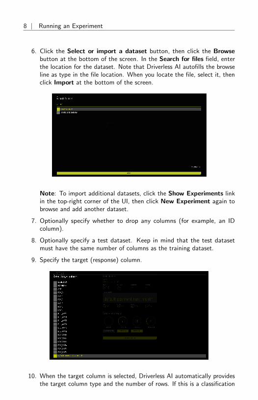
6. Click the Select or import a dataset button, then click the Browsebutton at the bottom of the screen. In the Search for files field, enterthe location for the dataset. Note that Driverless AI autofills the browseline as type in the file location. When you locate the file, select it, thenclick Import at the bottom of the screen.

Note: To import additional datasets, click the Show Experiments linkin the top-right corner of the UI, then click New Experiment again tobrowse and add another dataset.

7. Optionally specify whether to drop any columns (for example, an IDcolumn).

8. Optionally specify a test dataset. Keep in mind that the test datasetmust have the same number of columns as the training dataset.

9. Specify the target (response) column.

10. When the target column is selected, Driverless AI automatically providesthe target column type and the number of rows. If this is a classification

Running an Experiment | 9

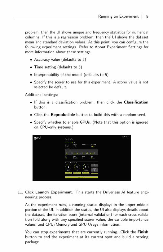
problem, then the UI shows unique and frequency statistics for numericalcolumns. If this is a regression problem, then the UI shows the datasetmean and standard deviation values. At this point, you can configure thefollowing experiment settings. Refer to About Experiment Settings formore information about these settings.

• Accuracy value (defaults to 5)

• Time setting (defaults to 5)

• Interpretability of the model (defaults to 5)

• Specify the scorer to use for this experiment. A scorer value is notselected by default.

Additional settings:

• If this is a classification problem, then click the Classificationbutton.

• Click the Reproducible button to build this with a random seed.

• Specify whether to enable GPUs. (Note that this option is ignoredon CPU-only systems.)

11. Click Launch Experiment. This starts the Driverless AI feature engi-neering process.

As the experiment runs, a running status displays in the upper middleportion of the UI. In addition the status, the UI also displays details aboutthe dataset, the iteration score (internal validation) for each cross valida-tion fold along with any specified scorer value, the variable importancevalues, and CPU/Memory and GPU Usage information.

You can stop experiments that are currently running. Click the Finishbutton to end the experiment at its current spot and build a scoringpackage.

10 | Running an Experiment

3.1 About Experiment Settings

This section describes the settings that are available when running an experi-ments.

Test Data

Test data is used to create test predictions only. This dataset is not used formodel scoring.

Dropped Columns

Dropped columns are columns that you do not want to be used as predictors inthe experiment.

Accuracy

The following table describes how the Accuracy value affects a Driverless AIexperiment.

The list below includes more information about the parameters that are usedwhen calculating accuracy.

• Max Rows: the maximum number of rows to use in model training.

Running an Experiment | 11

– For classification, stratified random sampling is performed

– For regression, random sampling is performed

• Ensemble Level: The level of ensembling done

– 0: single final model

– 1: 3 3-fold final models ensembled together

– 2: 5 5-fold final models ensembled together

• Target Transformation: Try target transformations and choose thetransformation that has the best score

– Possible transformations: identity, log, square, square root, inverse,Anscombe, logit, sigmoid

• Tune Parameters: Tune the parameters of the XGBoost model

– Only max depth tuned is tuned, and the range is 3 to 10

– Max depth chosen by penalized score, which is a combinationof the model’s accuracy and complexity

• Num Individuals: The number of individuals in the population for thegenetic algorithms

– Each individual is a gene. The more genes, the more combinationsof features are tried.

– Default is automatically determined. Typical values are 4 or 8.

• CV Folds: The number of cross validation folds done for each model

– If the problem is a classification problem, then stratified folds arecreated.

• Only First CV Model: Equivalent to splitting data into a training andtesting set

– Example: Setting CV Folds to 3 and Only First CV Model = Truemeans you are splitting the data into 66% training and 33% testing.

• Strategy: Feature selection strategy

– None: No feature selection

– FS: Feature selection permutations

12 | Interpreting a Model

Time

Interpretability

4 Interpreting a Model

After the status changes from RUNNING to COMPLETE, the UI provides youwith several options:

• Interpret this Model

• Score on Another Dataset

• Download (Holdout) Training Predictions (in csv format)

• Download Predictions (in csv format, available if a test dataset is used)

• Download Transformed Training Data (in csv format)

• Download Transformed Test Data (in csv format, available if a test datasetis used)

• Download Logs

• Download Scoring Package (a standalone Python scoring package forH2O Driverless AI)

• View Warnings (if any existed)

Interpreting a Model | 13

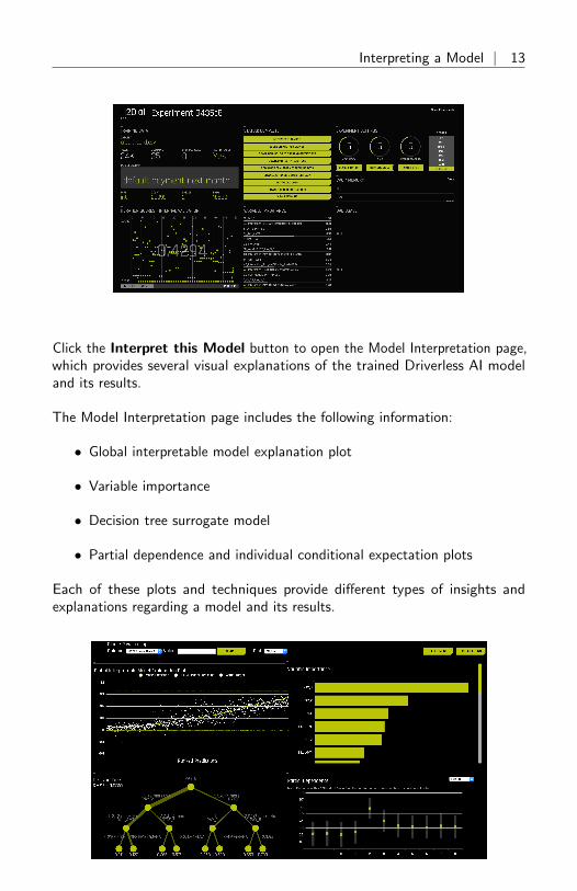
Click the Interpret this Model button to open the Model Interpretation page,which provides several visual explanations of the trained Driverless AI modeland its results.

The Model Interpretation page includes the following information:

• Global interpretable model explanation plot

• Variable importance

• Decision tree surrogate model

• Partial dependence and individual conditional expectation plots

Each of these plots and techniques provide different types of insights andexplanations regarding a model and its results.

14 | Interpreting a Model

4.1 K-LIME

4.1.1 The K-LIME Technique

K -LIME is a variant of the LIME technique proposed by Ribeiro at al [9]. K -LIME generates global and local explanations that increase the transparency ofthe Driverless AI model, and allow model behavior to be validated and debuggedby analyzing the provided plots, and comparing global and local explanationsto one-another, to known standards, to domain knowledge, and to reasonableexpectations.

K -LIME creates one global surrogate GLM on the entire training data andalso creates numerous local surrogate GLMs on samples formed from k-meansclusters in the training data. All penalized GLM surrogates are trained to modelthe predictions of the Driverless AI model. The number of clusters for localexplanations is chosen by a grid search in which the R2 between the DriverlessAI model predictions and all of the local K -LIME model predictions is maximized.The global and local linear model’s intercepts, coefficients, R2 values, accuracy,and predictions can all be used to debug and develop explanations for theDriverless AI model’s behavior.

The parameters of the global K -LIME model give an indication of overall linearvariable importance and the overall average direction in which an input variableinfluences the Driverless AI model predictions. The global model is also usedto generate explanations for very small clusters (N < 20) where fitting a locallinear model is inappropriate.

The in-cluster linear model parameters can be used to profile the local region,to give an average description of the important variables in the local region,and to understand the average direction in which an input variable affects theDriverless AI model predictions. For a point within a cluster, the sum of the locallinear model intercept and the products of each coefficient with their respectiveinput variable value are the K -LIME prediction. By disaggregating the K -LIMEpredictions into individual coefficient and input variable value products, thelocal linear impact of the variable can be determined. This product is sometimesreferred to as a reason code and is used to create explanations for the DriverlessAI model’s behavior.

In the following example, reason codes are created by evaluating and disaggre-gating a local linear model.

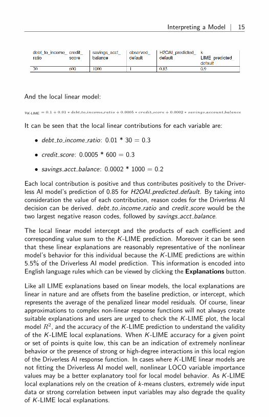
Given the row of input data with its corresponding Driverless AI and K -LIMEpredictions:

Interpreting a Model | 15

And the local linear model:

yK -LIME = 0.1 + 0.01 ∗ debt to income ratio + 0.0005 ∗ credit score + 0.0002 ∗ savings account balance

It can be seen that the local linear contributions for each variable are:

• debt to income ratio: 0.01 * 30 = 0.3

• credit score: 0.0005 * 600 = 0.3

• savings acct balance: 0.0002 * 1000 = 0.2

Each local contribution is positive and thus contributes positively to the Driver-less AI model’s prediction of 0.85 for H2OAI predicted default. By taking intoconsideration the value of each contribution, reason codes for the Driverless AIdecision can be derived. debt to income ratio and credit score would be thetwo largest negative reason codes, followed by savings acct balance.

The local linear model intercept and the products of each coefficient andcorresponding value sum to the K -LIME prediction. Moreover it can be seenthat these linear explanations are reasonably representative of the nonlinearmodel’s behavior for this individual because the K -LIME predictions are within5.5% of the Driverless AI model prediction. This information is encoded intoEnglish language rules which can be viewed by clicking the Explanations button.

Like all LIME explanations based on linear models, the local explanations arelinear in nature and are offsets from the baseline prediction, or intercept, whichrepresents the average of the penalized linear model residuals. Of course, linearapproximations to complex non-linear response functions will not always createsuitable explanations and users are urged to check the K -LIME plot, the localmodel R2, and the accuracy of the K -LIME prediction to understand the validityof the K -LIME local explanations. When K -LIME accuracy for a given pointor set of points is quite low, this can be an indication of extremely nonlinearbehavior or the presence of strong or high-degree interactions in this local regionof the Driverless AI response function. In cases where K -LIME linear models arenot fitting the Driverless AI model well, nonlinear LOCO variable importancevalues may be a better explanatory tool for local model behavior. As K -LIMElocal explanations rely on the creation of k-means clusters, extremely wide inputdata or strong correlation between input variables may also degrade the qualityof K -LIME local explanations.

16 | Interpreting a Model

4.1.2 The Global Interpretable Model Explanation Plot

This plot is in the upper-left quadrant of the UI. It shows Driverless AI modelpredictions and K -LIME model predictions in sorted order by the Driverless AImodel predictions. This graph is interactive. Hover over the Model Prediction,K-LIME Model Prediction, or Actual Target radio buttons to magnify theselected predictions. Or click those radio buttons to disable the view in thegraph. You can also hover over any point in the graph to view K -LIME reasoncodes for that value. By default, this plot shows information for the globalK -LIME model, but you can change the plot view to show local results froma specific cluster. The K -LIME plot also provides a visual indication of thelinearity of the Driverless AI model and the trustworthiness of the K -LIMEexplanations. The closer the local linear model approximates the DriverlessAI model predictions, the more linear the Driverless AI model and the moreaccurate the explanation generated by the K -LIME local linear models.

4.2 Global and Local Variable Importance

Variable importance measures the effect that a variable has on the predictionsof a model. Global and local variable importance values enable increasedtransparency in the Driverless AI model and enable validating and debugging ofthe Driverless AI model by comparing global model behavior to the local modelbehavior, and by comparing to global and local variable importance to knownstandards, domain knowledge, and reasonable expectations.

Interpreting a Model | 17

4.2.1 Global Variable Importance Technique

Global variable importance measures the overall impact of an input variable onthe Driverless AI model predictions while taking nonlinearity and interactionsinto consideration. Global variable importance values give an indication ofthe magnitude of a variable’s contribution to model predictions for all rows.Unlike regression parameters, they are often unsigned and typically not directlyrelated to the numerical predictions of the model. The reported global variableimportance values are calculated by aggregating the improvement in the split-criterion for a variable across all the trees in an ensemble. The aggregatedfeature importance values are then scaled between 0 and 1, such that the mostimportant feature has an importance value of 1.

4.2.2 Local Variable Importance Technique

Local variable importance describes how the combination of the learned modelrules or parameters and an individual row’s attributes affect a model’s predictionfor that row while taking nonlinearity and interactions into effect. Local variableimportance values reported here are based on a variant of the leave-one-covariate-out (LOCO) method (Lei et al, 2017 [8]).

In the LOCO-variant method, each local variable importance is found by re-scoring the trained Driverless AI model for each feature in the row of interest,while removing the contribution to the model prediction of splitting rules thatcontain that variable throughout the ensemble. The original prediction is thensubtracted from this modified prediction to find the raw, signed importancefor the feature. All local feature importance values for the row are then scaledbetween 0 and 1 for direct comparison with global variable importance values.

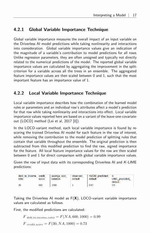
Given the row of input data with its corresponding Driverless AI and K -LIMEpredictions:

Taking the Driverless AI model as F(X), LOCO-variant variable importancevalues are calculated as follows.

First, the modified predictions are calculated:

F debt to income ratio = F (NA, 600, 1000) = 0.99

F credit score = F (30, NA, 1000) = 0.73

18 | Interpreting a Model

F savings acct balance = F (30, 600, NA) = 0.82

Second, the original prediction is subtracted from each modified prediction togenerate the unscaled local variable importance values:

LOCOdebt to income ratio = F debt to income ratio − 0.85 = 0.99 −0.85 = 0.14

LOCOcredit score = F credit score − 0.85 = 0.73− 0.85 = −0.12

LOCOsavings acct balance = F savings acct balance − 0.85 = 0.82 −0.85 = −0.03

Finally LOCO values are scaled between 0 and 1 by dividing each value for therow by the maximum value for the row and taking the absolute magnitude ofthis quotient.

Scaled(LOCOdebt to income ratio) = Abs(LOCO debt to income ratio/0.14) =1

Scaled(LOCOcredit score) = Abs(LOCO credit score/0.14) = 0.86

Scaled(LOCOsavings acct balance) = Abs(LOCO savings acct balance/0.14) =0.21

One drawback to these LOCO-variant variable importance values is, unlikeK -LIME, it is difficult to generate a mathematical error rate to indicate whenLOCO values may be questionable.

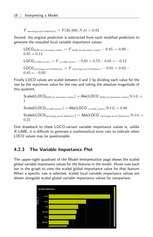
4.2.3 The Variable Importance Plot

The upper-right quadrant of the Model Interpretation page shows the scaledglobal variable importance values for the features in the model. Hover over eachbar in the graph to view the scaled global importance value for that feature.When a specific row is selected, scaled local variable importance values areshown alongside scaled global variable importance values for comparison.

Interpreting a Model | 19

4.3 Decision Tree Surrogate Model

4.3.1 The Decision Tree Surrogate Model Technique

The decision tree surrogate model increases the transparency of the DriverlessAI model by displaying an approximate flow-chart of the complex DriverlessAI model’s decision making process. The decision tree surrogate model alsodisplays the most important variables in the Driverless AI model and the mostimportant interactions in the Driverless AI model. The decision tree surrogatemodel can be used for visualizing, validating, and debugging the Driverless AImodel by comparing the displayed decision-process, important variables, andimportant interactions to known standards, domain knowledge, and reasonableexpectations.

A surrogate model is a data mining and engineering technique in which agenerally simpler model is used to explain another, usually more complex, modelor phenomenon. The decision tree surrogate is known to date back at leastto 1996 (Craven and Shavlik, [2]). The decision tree surrogate model hereis trained to predict the predictions of the more complex Driverless AI modelusing the of original model inputs. The trained surrogate model enables aheuristic understanding (i.e.,not a mathematically precise understanding) of themechanisms of the highly complex and nonlinear Driverless AI model.

4.3.2 The Decision Tree Surrogate Model Plot

The lower-left quadrant shows a decision tree surrogate for the generated model.The highlighted row shows the path to the highest probability leaf node andindicates the globally important variables and interactions that influence theDriverless AI model prediction for that row.

20 | Interpreting a Model

4.4 Partial Dependence and Individual ConditionalExpectation (ICE)

4.4.1 The Partial Dependence Technique

Partial dependence is a measure of the average model prediction with respectto an input variable. Partial dependence plots display how machine-learnedresponse functions change based on the values of an input variable of interest,while taking nonlinearity into consideration and averaging out the effects of allother input variables. Partial dependence plots are well-known and described inthe Elements of Statistical Learning (Hastie et all, 2001 [3]). Partial dependenceplots enable increased transparency in Driverless AI models and the ability tovalidate and debug Driverless AI models by comparing a variable’s averagepredictions across its domain to known standards, domain knowledge, andreasonable expectations.

4.4.2 The ICE Technique

Individual conditional expectation (ICE) plots, a newer and less well-knownadaptation of partial dependence plots, can be used to create more localizedexplanations for a single individual using the same basic ideas as partial depen-dence plots. ICE Plots were described by Goldstein et al (2015 [4]). ICE valuesare simply disaggregated partial dependence, but ICE is also a type of nonlinearsensitivity analysis in which the model predictions for a single row are measuredwhile a variable of interest is varied over its domain. ICE plots enable a userto determine whether the model’s treatment of an individual row of data isoutside one standard deviation from the average model behavior, whether thetreatment of a specific row is valid in comparison to average model behavior,known standards, domain knowledge, and reasonable expectations, and how amodel will behave in hypothetical situations where one variable in a selectedrow is varied across its domain.

Given the row of input data with its corresponding Driverless AI and K -LIMEpredictions:

Taking the Driverless AI model as F(X), assuming credit scores vary from 500to 800 in the training data, and that increments of 30 are used to plot the ICEcurve, ICE is calculated as follows:

Interpreting a Model | 21

ICEcredit score,500 = F (30, 500, 1000)

ICEcredit score,530 = F (30, 530, 1000)

ICEcredit score,560 = F (30, 560, 1000)

...

ICEcredit score,800 = F (30, 800, 1000)

The one-dimensional partial dependence plots displayed here do not take inter-actions into account. Large differences in partial dependence and ICE are anindication that strong variable interactions may be present. In this case partialdependence plots may be misleading because average model behavior may notaccurately reflect local behavior.

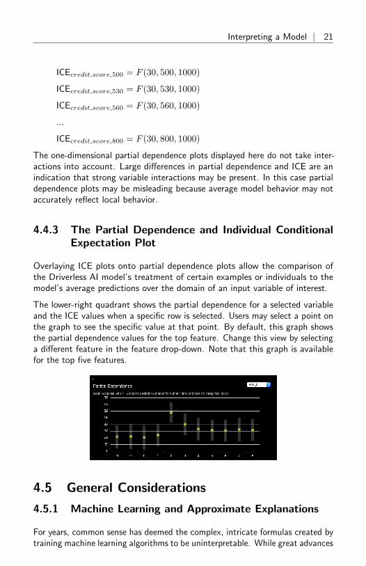
4.4.3 The Partial Dependence and Individual ConditionalExpectation Plot

Overlaying ICE plots onto partial dependence plots allow the comparison ofthe Driverless AI model’s treatment of certain examples or individuals to themodel’s average predictions over the domain of an input variable of interest.

The lower-right quadrant shows the partial dependence for a selected variableand the ICE values when a specific row is selected. Users may select a point onthe graph to see the specific value at that point. By default, this graph showsthe partial dependence values for the top feature. Change this view by selectinga different feature in the feature drop-down. Note that this graph is availablefor the top five features.

4.5 General Considerations

4.5.1 Machine Learning and Approximate Explanations

For years, common sense has deemed the complex, intricate formulas created bytraining machine learning algorithms to be uninterpretable. While great advances

22 | Interpreting a Model

have been made in recent years to make these often nonlinear, non-monotonic,and non-continuous machine-learned response functions more understandable(Hall et al, 2017 [6]), it is likely that such functions will never be as directly oruniversally interpretable as more traditional linear models.

Why consider machine learning approaches for inferential purposes? In general,linear models focus on understanding and predicting average behavior, whereasmachine-learned response functions can often make accurate, but more difficultto explain, predictions for subtler aspects of modeled phenomenon. In a sense,linear models create very exact interpretations for approximate models. Theapproach here seeks to make approximate explanations for very exact models.It is quite possible that an approximate explanation of an exact model mayhave as much, or more, value and meaning than the exact interpretations ofan approximate model. Moreover, the use of machine learning techniques forinferential or predictive purposes does not preclude using linear models forinterpretation (Ribeiro et al, 2016 [9]).

4.5.2 The Multiplicity of Good Models in Machine Learn-ing

It is well understood that for the same set of input variables and predictiontargets, complex machine learning algorithms can produce multiple accuratemodels with very similar, but not exactly the same, internal architectures(Brieman, 2001 [1]). This alone is an obstacle to interpretation, but when usingthese types of algorithms as interpretation tools or with interpretation tools it isimportant to remember that details of explanations will change across multipleaccurate models.

4.5.3 Expectations for Consistency Between ExplanatoryTechniques

• The decision tree surrogate is a global, nonlinear description of theDriverless AI model behavior. Variables that appear in the tree shouldhave a direct relationship with variables that appear in the global variableimportance plot. For certain, more linear Driverless AI models, variablesthat appear in the decision tree surrogate model may also have largecoefficients in the global K -LIME model.

• K -LIME explanations are linear, do not consider interactions, and representoffsets from the local linear model intercept. LOCO importance valuesare nonlinear, do consider interactions, and do not explicitly considera linear intercept or offset. LIME explanations and LOCO importance

Viewing Explanations | 23

values are not expected to have a direct relationship but can align roughlyas both are measures of a variable’s local impact on a model’s predictions,especially in more linear regions of the Driverless AI model’s learnedresponse function.

• ICE is a type of nonlinear sensitivity analysis which has a complex relation-ship to LOCO variable importance values. Comparing ICE to LOCO canonly be done at the value of the selected variable that actually appearsin the selected row of the training data. When comparing ICE to LOCOthe total value of the prediction for the row, the value of the variablein the selected row, and the distance of the ICE value from the averageprediction for the selected variable at the value in the selected row mustall be considered.

• ICE curves that are outside the standard deviation of partial dependencewould be expected to fall into less populated decision paths of the decisiontree surrogate; ICE curves that lie within the standard deviation of partialdependence would be expected to belong to more common decision paths.

• Partial dependence takes into consideration nonlinear, but average, behav-ior of the complex Driverless AI model without considering interactions.Variables with consistently high partial dependence or partial dependencethat swings widely across an input variable’s domain will likely also havehigh global importance values. Strong interactions between input variablescan cause ICE values to diverge from partial dependence values.

5 Viewing ExplanationsDriverless AI provides easy-to-read explanations for a completed model. Youcan view these by clicking the Explanations button in the upper-right cornerof the Model Interpretation page. Note that this button is only available forcompleted experiments. Click Close when you are done to return to the ModelInterpretations page.

The UI allows you to view global, cluster-specific, and local reason codes.

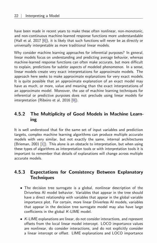
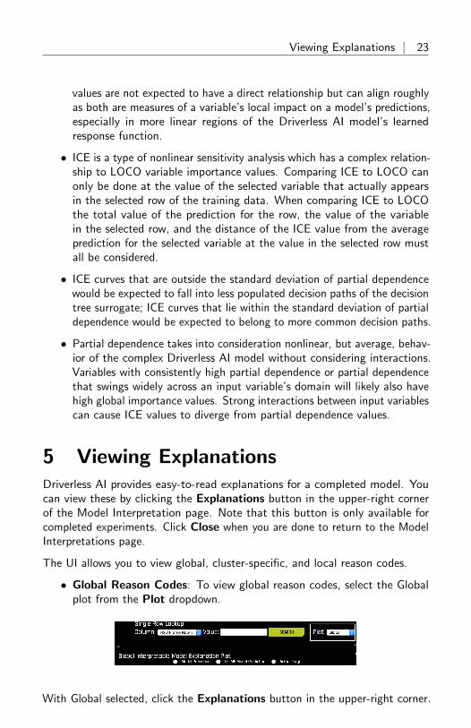
• Global Reason Codes: To view global reason codes, select the Globalplot from the Plot dropdown.

With Global selected, click the Explanations button in the upper-right corner.

24 | Viewing Explanations

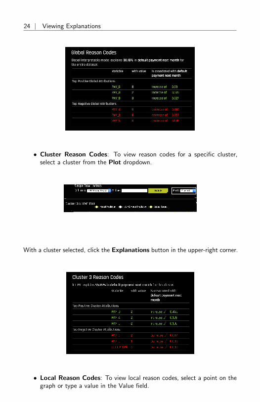
• Cluster Reason Codes: To view reason codes for a specific cluster,select a cluster from the Plot dropdown.

With a cluster selected, click the Explanations button in the upper-right corner.

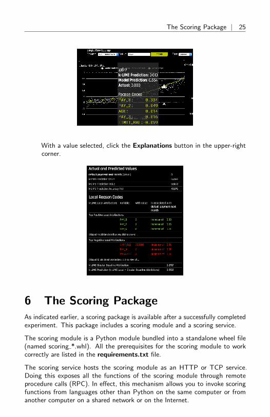
• Local Reason Codes: To view local reason codes, select a point on thegraph or type a value in the Value field.

The Scoring Package | 25

With a value selected, click the Explanations button in the upper-rightcorner.

6 The Scoring PackageAs indicated earlier, a scoring package is available after a successfully completedexperiment. This package includes a scoring module and a scoring service.

The scoring module is a Python module bundled into a standalone wheel file(named scoring *.whl). All the prerequisites for the scoring module to workcorrectly are listed in the requirements.txt file.

The scoring service hosts the scoring module as an HTTP or TCP service.Doing this exposes all the functions of the scoring module through remoteprocedure calls (RPC). In effect, this mechanism allows you to invoke scoringfunctions from languages other than Python on the same computer or fromanother computer on a shared network or on the Internet.

26 | The Scoring Package

The scoring service can be started in two modes:

• In TCP mode, the scoring service provides high-performance RPC callsvia Apache Thrift (https://thrift.apache.org/) using a binarywire protocol.

• In HTTP mode, the scoring service provides JSON-RPC 2.0 calls servedby Tornado (http://www.tornadoweb.org).

Scoring operations can be performed on individual rows (row-by-row) or inbatch mode (multiple rows at a time).

6.1 Prerequisites

The following are required in order to run the downloaded scoring package.

• Linux x86 64 environment

• Python 3.6

• Virtual Environment

• Apache Thrift (to run the TCP scoring service)

The scoring package has been tested on Ubuntu 16.04 and on 16.10+. Examplesof how to install these prerequisites are below:

Installing requirements on Ubuntu 16.10+

$ sudo apt install python3.6 python3.6-dev python3-pip python3-dev \python-virtualenv python3-virtualenv

Installing requirements on Ubuntu 16.4

$ sudo add-apt-repository ppa:deadsnakes/ppa$ sudo apt-get update$ sudo apt-get install python3.6 python3.6-dev python3-pip python3-dev \

python-virtualenv python3-virtualenv

Installing Thrift

Thrift is required to run the scoring service in TCP mode, but it is not re-quired to run the scoring module. The following steps are available on theThrift documentation site at: https://thrift.apache.org/docs/BuildingFromSource.

$ sudo apt-get install automake bison flex g++ git libevent-dev \libssl-dev libtool make pkg-config libboost-all-dev ant

$ wget https://github.com/apache/thrift/archive/0.10.0.tar.gz$ tar -xvf 0.10.0.tar.gz$ cd thrift-0.10.0$ ./bootstrap.sh$ ./configure

The Scoring Package | 27

$ make$ sudo make install

6.2 Scoring Package Files

The scoring-package folder includes the following notable files:

• example.py: An example Python script demonstrating how to importand score new records.

• run example.sh: Runs example.py (also sets up a virtualenv with pre-requisite libraries).

• server.py: A standalone TCP/HTTP server for hosting scoring services.

• run tcp server.sh: Runs TCP scoring service (runs server.py).

• run http server.sh: Runs HTTP scoring service (runs server.py).

• example client.py: An example Python script demonstrating how tocommunicate with the scoring server.

• run tcp client.sh: Demonstrates how to communicate with the scoringservice via TCP (runs example client.py).

• run http client.sh: Demonstrates how to communicate with the scoringservice via HTTP (using curl).

6.3 Examples

This section provides examples showing how to run the scoring module and howto run the scoring service in TCP and HTTP mode.

Before running these examples, be sure that the scoring package is alreadydownloaded and unzipped:

1. On the completed Experiment page, click on the Download ScoringPackage button to download the scorer.zip file for this experiment ontoyour local machine.

28 | The Scoring Package

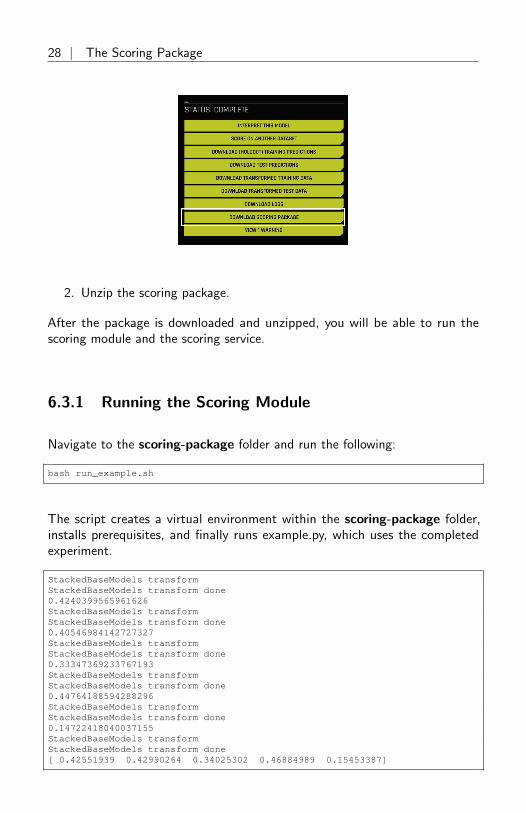
2. Unzip the scoring package.

After the package is downloaded and unzipped, you will be able to run thescoring module and the scoring service.

6.3.1 Running the Scoring Module

Navigate to the scoring-package folder and run the following:

bash run_example.sh

The script creates a virtual environment within the scoring-package folder,installs prerequisites, and finally runs example.py, which uses the completedexperiment.

StackedBaseModels transformStackedBaseModels transform done0.4240399565961626StackedBaseModels transformStackedBaseModels transform done0.40546984142727327StackedBaseModels transformStackedBaseModels transform done0.33347369233767193StackedBaseModels transformStackedBaseModels transform done0.44764188594288296StackedBaseModels transformStackedBaseModels transform done0.14722418040037155StackedBaseModels transformStackedBaseModels transform done[ 0.42551939 0.42990264 0.34025302 0.46884989 0.15453387]

The Scoring Package | 29

6.3.2 Running the Scoring Service - TCP Mode

TCP mode allows you to use the scoring service from any language supportedby Thrift, including C, C++, Cocoa, D, Dart, Delphi, Go, Haxe, Java, Node.js,Lua, perl, PHP, Python, Ruby, and Smalltalk.

To start the scoring service in TCP mode, generate the Thrift bindings once,and then run the server. Note that the Thrift compiler is only required atbuild-time. It is not a run time dependency, i.e. once the scoring services arebuilt and tested, you do not need to repeat this installation process on themachines where the scoring services are intended to be deployed.

# See the run_tcp_server.sh file for a complete example.$ thrift --gen py scoring.thrift$ python server.py --mode=tcp --port=9090

Call the scoring service by generating the Thrift bindings for your language ofchoice, then make RPC calls via TCP sockets using Thrift’s buffered transportin conjunction with its binary protocol.

See the run_tcp_client.sh and example_client.py files for a complete example.$ thrift --gen py scoring.thrift

socket = TSocket.TSocket(’localhost’, 9090)transport = TTransport.TBufferedTransport(socket)protocol = TBinaryProtocol.TBinaryProtocol(transport)client = ScoringService.Client(protocol)transport.open()row = Row()row.sepalLen = 7.416 # sepal_lenrow.sepalWid = 3.562 # sepal_widrow.petalLen = 1.049 # petal_lenrow.petalWid = 2.388 # petal_widscores = client.score(row)transport.close()

Note that you can reproduce the exact same results from other languages. Forexample, to run the scoring service in Java, use:

$ thrift --gen java scoring.thrift

6.3.3 Running the Scoring Service - HTTP Mode

The HTTP mode allows you to use the scoring service using plaintext JSON-RPC calls. This is usually less performant compared to Thrift, but has theadvantage of being usable from any HTTP client library in your language ofchoice, without any dependency on Thrift.

See http://www.jsonrpc.org/specification for JSON-RPC docu-mentation.

30 | Viewing Experiments

To start the scoring service in HTTP mode:

# See run_http_server.sh for a complete example$ python server.py --mode=http --port=9090

To invoke scoring methods, compose a JSON-RPC message and make a HTTPPOST request to http://host:port/rpc as follows:

# See run_http_client.sh for a complete example$ curl http://localhost:9090/rpc \--header "Content-Type: application/json" \--data @- <<EOF{"id": 1,"method": "score","params": {"row": [ 7.486, 3.277, 4.755, 2.354 ]

}}EOF

Similarly, you can use any HTTP client library to reproduce the above result.For example, from Python, you can use the requests module as follows:

import requestsrow = [7.486, 3.277, 4.755, 2.354]req = dict(id=1, method=’score’, params=dict(row=row))res = requests.post(’http://localhost:9090/rpc’, data=req)print(res.json()[’result’])

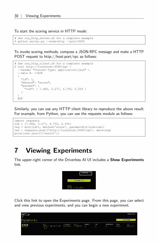
7 Viewing ExperimentsThe upper-right corner of the Driverless AI UI includes a Show Experimentslink.

Click this link to open the Experiments page. From this page, you can selectand view previous experiments, and you can begin a new experiment.

Visualizing Datasets | 31

8 Visualizing DatasetsWhile viewing experiments, click the Visualize Datasets link in the upper-rightcorner.

The Datasets page shows a list of the datasets that you’ve imported.

Select a dataset to view the following graphical representations. Note that thelist of graphs that displays can vary based on the information in your dataset.

• Clumpy Scatterplots: Clumpy scatterplots are 2D plots with evidentclusters. These clusters are regions of high point density separated fromother regions of points. The clusters can have many different shapes andare not necessarily circular. All possible scatterplots based on pairs offeatures (variables) are examined for clumpiness. The displayed plots areranked according to the RUNT statistic. Note that the test for clumpinessis described in Hartigan, J. A. and Mohanty, S. (1992), ”The RUNT

32 | Visualizing Datasets

test for multimodality,” Journal of Classification, 9, 63–70 ([7]). Thealgorithm implemented here is described in Wilkinson, L., Anand, A., andGrossman, R. (2005), ”Graph-theoretic Scagnostics,” in Proceedings ofthe IEEE Information Visualization 2005, pp. 157–164 ([11]).

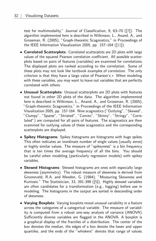
• Correlated Scatterplots: Correlated scatterplots are 2D plots with largevalues of the squared Pearson correlation coefficient. All possible scatter-plots based on pairs of features (variables) are examined for correlations.The displayed plots are ranked according to the correlation. Some ofthese plots may not look like textbook examples of correlation. The onlycriterion is that they have a large value of Pearson’s r. When modelingwith these variables, you may want to leave out variables that are perfectlycorrelated with others.

• Unusual Scatterplots: Unusual scatterplots are 2D plots with featuresnot found in other 2D plots of the data. The algorithm implementedhere is described in Wilkinson, L., Anand, A., and Grossman, R. (2005),”Graph-theoretic Scagnostics,” in Proceedings of the IEEE InformationVisualization 2005, pp. 157-164. Nine scagnostics (”Outlying”, ”Skewed”,”Clumpy”, ”Sparse”, ”Striated”, ”Convex”, ”Skinny”, ”Stringy”, ”Corre-lated”) are computed for all pairs of features. The scagnostics are thenexamined for outlying values of these scagnostics and the correspondingscatterplots are displayed.

• Spikey Histograms: Spikey histograms are histograms with huge spikes.This often indicates an inordinate number of single values (usually zeros)or highly similar values. The measure of ”spikeyness” is a bin frequencythat is ten times the average frequency of all the bins. You shouldbe careful when modeling (particularly regression models) with spikeyvariables.

• Skewed Histograms: Skewed histograms are ones with especially largeskewness (asymmetry). The robust measure of skewness is derived fromGroeneveld, R.A. and Meeden, G. (1984), ”Measuring Skewness andKurtosis.” The Statistician, 33, 391-399 ([5]). Highly skewed variablesare often candidates for a transformation (e.g., logging) before use inmodeling. The histograms in the output are sorted in descending orderof skewness.

• Varying Boxplots: Varying boxplots reveal unusual variability in a featureacross the categories of a categorical variable. The measure of variabil-ity is computed from a robust one-way analysis of variance (ANOVA).Sufficiently diverse variables are flagged in the ANOVA. A boxplot isa graphical display of the fractiles of a distribution. The center of thebox denotes the median, the edges of a box denote the lower and upperquartiles, and the ends of the ”whiskers” denote that range of values.

Visualizing Datasets | 33

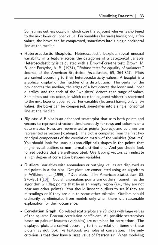
Sometimes outliers occur, in which case the adjacent whisker is shortenedto the next lower or upper value. For variables (features) having only a fewvalues, the boxes can be compressed, sometimes into a single horizontalline at the median.

• Heteroscedastic Boxplots: Heteroscedastic boxplots reveal unusualvariability in a feature across the categories of a categorical variable.Heteroscedasticity is calculated with a Brown-Forsythe test: Brown, M.B. and Forsythe, A. B. (1974), ”Robust tests for equality of variances.”Journal of the American Statistical Association, 69, 364-367. Plotsare ranked according to their heteroscedasticity values. A boxplot is agraphical display of the fractiles of a distribution. The center of thebox denotes the median, the edges of a box denote the lower and upperquartiles, and the ends of the ”whiskers” denote that range of values.Sometimes outliers occur, in which case the adjacent whisker is shortenedto the next lower or upper value. For variables (features) having only a fewvalues, the boxes can be compressed, sometimes into a single horizontalline at the median.

• Biplots: A Biplot is an enhanced scatterplot that uses both points andvectors to represent structure simultaneously for rows and columns of adata matrix. Rows are represented as points (scores), and columns arerepresented as vectors (loadings). The plot is computed from the first twoprincipal components of the correlation matrix of the variables (features).You should look for unusual (non-elliptical) shapes in the points thatmight reveal outliers or non-normal distributions. And you should lookfor red vectors that are well-separated. Overlapping vectors can indicatea high degree of correlation between variables.

• Outliers: Variables with anomalous or outlying values are displayed asred points in a dot plot. Dot plots are constructed using an algorithmin Wilkinson, L. (1999). ”Dot plots.” The American Statistician, 53,276–281 ([10]). Not all anomalous points are outliers. Sometimes thealgorithm will flag points that lie in an empty region (i.e., they are notnear any other points). You should inspect outliers to see if they aremiscodings or if they are due to some other mistake. Outliers shouldordinarily be eliminated from models only when there is a reasonableexplanation for their occurrence.

• Correlation Graph: Correlated scatterplots are 2D plots with large valuesof the squared Pearson correlation coefficient. All possible scatterplotsbased on pairs of features (variables) are examined for correlations. Thedisplayed plots are ranked according to the correlation. Some of theseplots may not look like textbook examples of correlation. The onlycriterion is that they have a large value of Pearson’s r. When modeling

34 | Visualizing Datasets

with these variables, you may want to leave out variables that are perfectlycorrelated with others.

• Radar Plot: A Radar Plot is a two-dimensional graph that is used forcomparing multiple variables. Each variable has its own axis that startsfrom the center of the graph. The data are standardized on each variablebetween 0 and 1 so that values can be compared across variables. Eachprofile, which usually appears in the form of a star, connects the valueson the axes for a single observation. Multivariate outliers are representedby red profiles. The Radar Plot is the polar version of the popular ParallelCoordinates plot. The polar layout enables us to represent more variablesin a single plot.

• Data Heatmap: The heatmap graphic is constructed from the transposeddata matrix. Rows of the heatmap represent variables, and columnsrepresent cases (instances). The data are standardized before display sothat small values are blue-ish and large values are red-ish. The rows andcolumns are permuted via a singular value decomposition (SVD) of thedata matrix so that similar rows and similar columns are near each other.

• Missing Values Heatmap: The missing values heatmap graphic isconstructed from the transposed data matrix. Rows of the heatmaprepresent variables and columns represent cases (instances). The data arecoded into the values 0 (missing) and 1 (nonmissing). Missing values arecolored red and nonmissing values are left blank (white). The rows andcolumns are permuted via a singular value decomposition (SVD) of thedata matrix so that similar rows and similar columns are near each other.

The images on this page are thumbnails. You can click on any of the graphs toview and download a full-scale image.

About Driverless AI Transformations | 35

9 About Driverless AI TransformationsTransformations in Driverless AI are applied to columns in the data. Thetransformers create the engineered features.

In this section, we will describe the transformations using the example ofpredicting house prices on the example dataset.

9.1 Frequent Transformer

• the count of each categorical value in the dataset

• the count can be either the raw count or the normalized count

There are 4,500 properties in this dataset with state = NY.

9.2 Bulk Interactions Transformer

• add, divide, multiply, and subtract two columns in the data

There is one more bedroom than there are number of bathrooms for thisproperty.

9.3 Truncated SVD Numeric Transformer

• truncated SVD trained on selected numeric columns of the data

• the components of the truncated SVD will be new features

36 | About Driverless AI Transformations

The first component of the truncated SVD of the columns Price, Number ofBeds, Number of Baths.

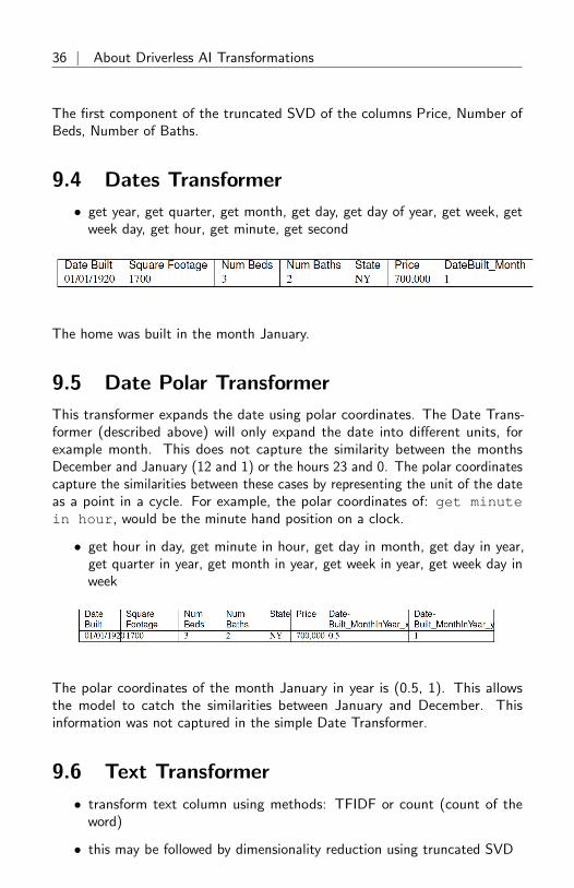
9.4 Dates Transformer

• get year, get quarter, get month, get day, get day of year, get week, getweek day, get hour, get minute, get second

The home was built in the month January.

9.5 Date Polar Transformer

This transformer expands the date using polar coordinates. The Date Trans-former (described above) will only expand the date into different units, forexample month. This does not capture the similarity between the monthsDecember and January (12 and 1) or the hours 23 and 0. The polar coordinatescapture the similarities between these cases by representing the unit of the dateas a point in a cycle. For example, the polar coordinates of: get minutein hour, would be the minute hand position on a clock.

• get hour in day, get minute in hour, get day in month, get day in year,get quarter in year, get month in year, get week in year, get week day inweek

The polar coordinates of the month January in year is (0.5, 1). This allowsthe model to catch the similarities between January and December. Thisinformation was not captured in the simple Date Transformer.

9.6 Text Transformer

• transform text column using methods: TFIDF or count (count of theword)

• this may be followed by dimensionality reduction using truncated SVD

About Driverless AI Transformations | 37

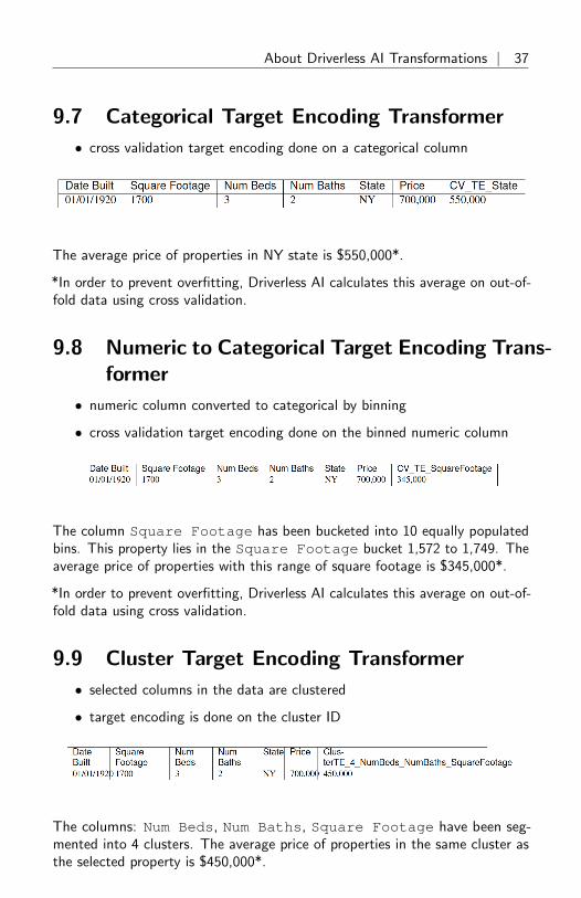
9.7 Categorical Target Encoding Transformer

• cross validation target encoding done on a categorical column

The average price of properties in NY state is $550,000*.

*In order to prevent overfitting, Driverless AI calculates this average on out-of-fold data using cross validation.

9.8 Numeric to Categorical Target Encoding Trans-former

• numeric column converted to categorical by binning

• cross validation target encoding done on the binned numeric column

The column Square Footage has been bucketed into 10 equally populatedbins. This property lies in the Square Footage bucket 1,572 to 1,749. Theaverage price of properties with this range of square footage is $345,000*.

*In order to prevent overfitting, Driverless AI calculates this average on out-of-fold data using cross validation.

9.9 Cluster Target Encoding Transformer

• selected columns in the data are clustered

• target encoding is done on the cluster ID

The columns: Num Beds, Num Baths, Square Footage have been seg-mented into 4 clusters. The average price of properties in the same cluster asthe selected property is $450,000*.

38 | Using the Driverless AI Python Client

*In order to prevent overfitting, Driverless AI calculates this average on out-of-fold data using cross validation.

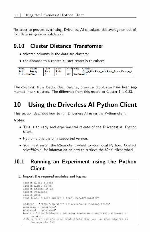
9.10 Cluster Distance Transformer

• selected columns in the data are clustered

• the distance to a chosen cluster center is calculated

The columns: Num Beds, Num Baths, Square Footage have been seg-mented into 4 clusters. The difference from this record to Cluster 1 is 0.83.

10 Using the Driverless AI Python ClientThis section describes how to run Driverless AI using the Python client.

Notes:

• This is an early and experimental release of the Driverless AI Pythonclient.

• Python 3.6 is the only supported version.

• You must install the h2oai client wheel to your local Python. Contactsales@h2o.ai for information on how to retrieve the h2oai client wheel.

10.1 Running an Experiment using the PythonClient

1. Import the required modules and log in.

import h2oai_clientimport numpy as npimport pandas as pdimport requestsimport mathfrom h2oai_client import Client, ModelParameters

address = ’http://ip_where_driverless_is_running:12345’username = ’username’password = ’password’h2oai = Client(address = address, username = username, password =

password)# Be sure to use the same credentials that you use when signing in

through the GUI

Using the Driverless AI Python Client | 39

2. Upload training and testing datasets from the Driverless AI **/data**folder.

train_path = ’/data/CreditCard/CreditCard-train.csv’test_path = ’/data/CreditCard/CreditCard-test.csv’

train = h2oai.create_dataset_sync(train_path)test = h2oai.create_dataset_sync(test_path)

3. Set the target (response) column and any ignored column or columns.

# set the parameters you want to pass to the UItarget = "default payment next month"drop_cols = [’ID’]

4. Specify the experiment settings. Refer to the :ref:‘experimentsettings‘ formore information about these settings.

# Pre-set parameters to pass modelis_classification = Trueenable_gpus = Trueseed=Truescorer_str = ’auc’

# Pre-sent accuracy knobsaccuracy_value = 5time_value = 5interpretability = 1

5. Launch the experiment to run feature engineering and final model training.In addition to the settings previously defined, be sure to also specify theimported training dataset. Adding a test dataset is optional.

experiment = h2oai.start_experiment_sync(ModelParameters(dataset_key=train.key,testset_key=test.key,target_col=target,is_classification=is_classification,cols_to_drop=drop_cols,enable_gpus=enable_gpus,seed=seed,accuracy=accuracy_value,time= time_value,interpretability=interpretability,scorer=scorer_str

))

6. View the results for an iteration. Note that the Web UI shows a graph ofthe iteration scores. You can retrieve the scores of each iteration from theexperiment object using the Python client. The example below retrievesthe score for the last iteration:

score = experiment.iteration_data[-1].scores # gets the ScoresTablescore = score.score[-1]print(score)

0.7875823819933607

40 | Using the Driverless AI Python Client

7. View the final model score for the train and test datasets. When featureengineering is complete, an ensemble model can be built depending onthe accuracy setting. The experiment object also contains the score onthe train and test data for this ensemble model.

print("Final Model Score on Train Data: " + str(round(experiment.train_score, 3)))

print("Final Model Score on Test Data: " + str(round(experiment.test_score, 3)))

Final Model Score on Train Data: 0.782Final Model Score on Test Data: 0.803

8. Download the test predictions.

h2oai.download(src_path = experiment.test_predictions_path, dest_dir =".")

’./test_preds.csv’

test_preds = pd.read_csv("./test_preds.csv")test_preds.head()

default payment next month.10 0.5148501 0.1367382 0.0624333 0.4819174 0.126809

10.2 Access an Experiment Object that was Runthrough the Web UI

It is also possible to use the Python API to examine an experiment that wasstarted through the Web UI using the experiment key.

You can get a pointer to the experiment by referencing the experiment key inthe Web UI.

experiment = h2oai.get_model_job("56507f").entity

10.3 Score on New Data

You can use the python API to score on new data. This is equivalent to theSCORE ON ANOTHER DATASET button in the Web UI. The example belowscores on the test data and then downloads the predictions.

Pass in any dataset that has the same columns as the original training set. If youpassed a test set during the H2OAI model building step, the predictions alreadyexist. Its path can be found with experiment.test predictions path.

FAQ | 41

prediction = h2oai.make_prediction_sync(experiment.key, test_path)pred_path = h2oai.download(prediction.predictions_csv_path, ’.’)pred_table = pd.read_csv(pred_path)pred_table.head()

default payment next month.10 0.5148501 0.1367382 0.0624333 0.4819174 0.126809

11 FAQHow does Driverless AI detect the ID column?

The ID column logic is that the column is named ’id’, ’Id’, ’ID’ or ’iD’ exactly.(It does not check the number of unique values.) For now, if you want to ensurethat your ID column is downloaded with the predictions, then you would wantto name it one of those names.

How can you download the predictions onto the machine where Driver-less AI is running?

When you select ”Score on Another Dataset” the predictions will be automati-cally downloaded to the machine where Driverless AI is running. It will be savedin the following locations:

• Training Data Predictions: tmp/experiment name/train preds.csv

• Testing Data Predictions: tmp/experiment name/test preds.csv

• New Data Predictions: tmp/experiment name/automatically generated name.Note that the automatically generated name will match the name of thefile downloaded to your local computer.

If I drop several columns from Train data set, will Driveless AI under-stand that it needs to drop the same columns from Test data set?

If you drop columns from the dataset, Driverless AI will do the same on thetest dataset.

How can I change my username and password?

The username and password is tied to the experiments you have created. Forexample, if I log in with the username/password: megan/megan and start anexperiment, then I would need to log back in with the same username andpassword to see those experiments. The username and password, however, doesnot limit your access to Driverless AI. If you want to use a new user name and

42 | References

password, you can log in again with a new username and password, but keep inmind that you won’t see your old experiments.

12 Have Questions?If you have questions about using Driverless AI, post them on Stack Over-flow using the h2o tag at http://stackoverflow.com/questions/tagged/h2o.

13 References

1. L. Breiman. Statistical modeling: The two cultures (with commentsand a rejoinder by the author). Statistical Science, 16(3), 2001. URLhttps://projecteuclid.org/euclid.ss/1009213726

2. M. W. Craven and J. W. Shavlik. Extracting tree-structured represen-tations of trained networks. Advances in Neural Information Process-ing Systems, 1996. URL http://papers.nips.cc/paper/1152-extracting-tree-structured-representations-of-trained-networks.pdf

3. J. Friedman, T. Hastie, and R. Tibshirani. The Elements of StatisticalLearning. Springer, New York, 2001. URL https://web.stanford.edu/˜hastie/ElemStatLearn/printings/ESLII_print12.pdf

4. A. Goldstein, A. Kapelner, J. Bleich, and E. Pitkin. Peeking inside the blackbox: Visualizing statistical learning with plots of individual conditionalexpectation. Journal of Computational and Graphical Statistics, 24(1),2015

5. R. A. Groeneveld and G. Meeden. Measuring Skewness and Kurtosis.Journal of the Royal Statistical Society. Series D (The Statistician), 33(4):391–399, December 1984

6. P. Hall, W. Phan, and S. S. Ambati. Ideas on interpreting machinelearning. O’Reilly Ideas, 2017. URL https://www.oreilly.com/ideas/ideas-on-interpreting-machine-learning

7. J. Hartigan and S. Mohanty. The RUNT test for Multimodality.Journal of Classification, 9(1):63–70, January 1992

8. J. Lei, M. G’Sell, A. Rinaldo, R. J. Tibshirani, and L. Wasserman.Distribution-free predictive inference for regression. Journal of the Amer-

Authors | 43

ican Statistical Association just-accepted, 2017. URL http://www.stat.cmu.edu/˜ryantibs/papers/conformal.pdf

9. M. T. Ribeiro, S. Singh, and C. Guestrin. Why should I trust you?:Explaining the predictions of any classifier. In Proceedings of the 22ndACM SIGKDD International Conference on Knowledge Discovery andData Mining, pages 1135–1144. ACM, 2016. URL http://www.kdd.org/kdd2016/papers/files/rfp0573-ribeiroA.pdf

10. L. Wilkinson. Dot Plots. The American Statistician, 53(3):276–281,1999

11. L. Wilkinson, A. Anand, and R. Grossman. ”Graph-theoretic Scagnostics,”in Proceedings of the IEEE Information Visualization. INFOVIS ’05. IEEEComputer Society, Washington, DC, USA, 2005

14 AuthorsPatrick Hall

Patrick Hall is senior director for data science products at H2O.ai where hefocuses mainly on model interpretability. Patrick is also currently an adjunctprofessor in the Department of Decision Sciences at George Washington Univer-sity, where he teaches graduate classes in data mining and machine learning.Prior to joining H2O.ai, Patrick held global customer facing roles and researchand development roles at SAS Institute.

Follow him on Twitter: @jpatrickhall

Megan Kurka

Megan is a customer data scientist at H2O.ai. Prior to working at H2O.ai,she worked as a data scientist building products driven by machine learning forB2B customers. Megan has experience working with customers across multipleindustries, identifying common problems, and designing robust and automatedsolutions.

Angela Bartz

Angela is the doc whisperer at H2O.ai. With extensive experience in technicalcommunication, she brings our products to life by documenting the features andfunctionality of the entire suite of H2O products. Having worked for companiesboth large and small, she is an expert at understanding her audience andtranslating complex ideas into consumable documents. Angela has a BA degreein English from the University of Detroit Mercy.