using heuristics and genetic algorithms for large-scale
TRANSCRIPT

261ISSN 1746-7659, England, UK Journal of Information and Computing Science
Vol. 2, No. 4, 2007, pp. 261-280
Using Heuristics and Genetic Algorithms for Large-scale Database Query Optimization
Zehai Zhou +
Department of FACIS, University of Houston – Downtown, Houston, TX 77002, USA (Received March 31, 2007, accepted May 11, 2007)
Abstract. Distributed database system technology is one of the major developments in information technology area. It will continue to have a very significant impact on data processing in the upcoming years because distributed database systems have many potential advantages over centralized systems for geographically distributed organizations. The continuing interest in distributed database systems in the research community and the marketplace and the introduction of many commercial products indicate that distributed database systems will play a more important role in data processing and eventually will replace centralized systems as the major database technology in the future. The availability of high speed communication networks and, especially, the phenomenal popularity of the Internet and the intranets will undoubtedly speed up the transition process. Some challenging problems must be solved before the full potential benefits of distributed database technology can be realized. Among them is query processing (including query optimization), one of the most important issues in distributed database system design. The query optimization problem in large-scale distributed databases is NP-hard in nature and difficult to solve. In this study, the query optimization problem is reduced to a join ordering problem similar to a variant of traveling salesman problem. We explored several heuristics and a genetic algorithm for solving the join ordering problem. Some computational experiments on these algorithms were conducted and solution qualities compared. The computation experiments show that heuristics and genetic algorithms are viable methods for solving query optimization problem in large scale distributed database systems.
Keywords: heuristics, genetic algorithm, NP-Hard, large scale database, query optimization, travelling salesman problem
1. Introduction A distributed database is a collection of multiple, logically interrelated databases distributed over a
computer network. Distributed database systems have many very promising potential advantages, such as improved reliability and availability, improved performance, shareability, expandability, and local autonomy, among others. To materialize the full potential benefits of distributed database technology, a series of technical problems have to be solved. Distributed query processing is among the most important and fundamental issues that must be appropriately addressed. Query processing includes designing algorithms that analyze queries and convert the queries into a set of data manipulation operations. An important aspect of query processing is query optimization. The distributed query optimization problem is NP-hard in nature and notoriously difficult to solve, which makes finding good solution methods and especially efficient (fast) and effective (generates close to optimal solutions) heuristics a high priority.
In query processing, previous research was limited to a small number of joins; we have investigated the query optimization problem with large join queries and tried to address the following questions:
1. What are the unique characteristics of the query optimization problem in large scale distributed databases?
2. What solution methods can be used/developed to solve the query optimization problem? How efficient/effective are those algorithms?
Our major objective is to advance the understanding of query processing in large-scale distributed database systems. To achieve this goal, we undertake the following tasks: to analyze the most important
+ Corresponding author. Tel.: +1-7137-222 5376; fax: +1-713-226 5238. E-mail address: [email protected].
Published by World Academic Press, World Academic Union

Z. Zhou: Using Heuristics and Genetic Algorithms for Large-scale Database Query Optimization 262
issues related to the problem, to model the problem, taking into consideration the most important factors, to propose some solution methods for these models, and, finally, to conduct computational experiments and compare the results to determine the effectiveness and efficiency of the solution techniques (algorithms). We believe that the development of the comprehensive models for the query optimization in large-scale systems, as well as finding effective and/or efficient solution techniques to solve the problems that have been identified are important and will contribute to the use of and research on distributed database technology.
The major task of query processing is to find a strategy (or strategies) for executing each query over the network in the most cost-effective and efficient way, taking into consideration of some important factors such as the distribution of the data, communication cost, and the lack of sufficient locally available information. Query optimization refers to the process of ensuring that either the total cost or the total response time for a query is minimized. The choices to be made by a query optimizer sub-module of the query processor include: (i) the order of executing (relational) operations; (ii) the access methods for the pertinent relations; (iii) the algorithms for carrying out the operations (in particular, relational joins); (iv) the order of data movements between sites. A good measure of resource consumption is the total cost that will be incurred in processing the query. In a distributed database system, the total cost to be minimized usually includes: (i) CPU; (ii) I/O; (iii) communication costs.
Query optimization in general and the selection of join order (the sequence in which relations are joined) in particular are critical to performance of and therefore the success of practical relational database management information systems. Query optimization has been an active area of research ever since the dawn of the development of database management systems. For good surveys on query optimization and closely related issues, please refer to [7] and [14]. For the complexity of query optimization for different kinds of query types with different assumptions, please refer to [10] and [17].
A query optimizer selects among the many alternative query execution plans (QEPs), the one with the least estimated execution cost, according to a given cost function. The objective functions of query optimization may take many different forms. One may try to find a query evaluation plan that optimizes the most relevant performance measures, such as the response time, CPU, I/O, and network time and efforts, memory or storage costs, resources usage (e.g. energy consumption for battery-powered mobile systems), a combination of the above, or some other performance measures.
The complexity of query optimization is basically determined by the number of alternative QEPs, which grows exponentially with the number of relations involved in the query. Consequently, enumerative optimization strategies are prohibitively expensive and therefore unacceptable as the query sizes grow. Moreover, a database management system usually supports a variety of join methods (algorithms) for processing joins and a variety of indices (data structures) for accessing individual relations, which increase the options (complexity) even further. All query optimization algorithms primarily deal with the join queries. These are also the scope of this research.
Traditional query optimizers expect to deal with queries involving only a small number of relations, usually requiring less than 10 join operations and therefore have relied on the use of enumerative optimization strategies [8, 9, 16, 18] (e.g. dynamic programming) that consider most of the alternatives if not all. Dynamic programming (as well as other enumerative optimization techniques) finds an optimal plan. But the time complexity of these algorithms is O(2N) where N is the number of joins involved. The combinatorial explosion in execution time used by enumerative type algorithms limits the complexity of the queries that can be handled using enumerative optimization strategies to about 15 (20) joins on even the powerful processors. However, it is expected that the query complexity will continue to grow, driven by the intelligent programs that have the capability to generate queries requiring a large number of joins and deeper nesting of virtual relation definitions through views. In addition, some new applications are now emerging, such as expert systems/knowledge based systems, decision support systems, object-oriented systems, deductive systems, that are often built on top of relational systems. These applications, plus engineering, statistic and scientific systems, typically require the processing of more complex queries that involve many relations and a large number of joins. In other words, we are expecting queries much more complex both in the number of operands (relations) and in the diversity and complexity of operators in the query.
2. Models for Query Optimization
JIC email for contribution: [email protected]
Journal of Information and Computing Science, 2 (2007) 4, pp 261-280
263
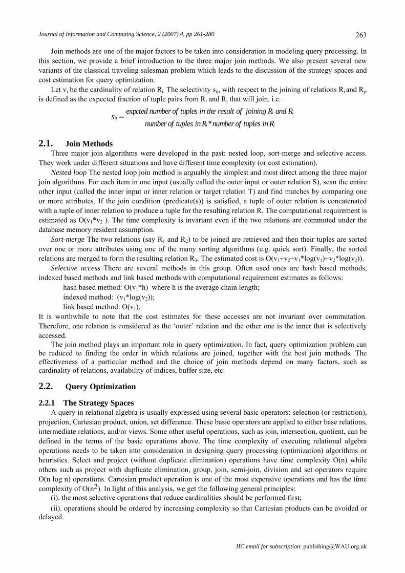
Join methods are one of the major factors to be taken into consideration in modeling query processing. In this section, we provide a brief introduction to the three major join methods. We also present several new variants of the classical traveling salesman problem which leads to the discussion of the strategy spaces and cost estimation for query optimization.
Let vi be the cardinality of relation Ri. The selectivity sij, with respect to the joining of relations Ri and Rj, is defined as the expected fraction of tuple pairs from Ri and Rj that will join, i.e.
exp*
i j
i j
ijcted number of tuples in the result of joining R and R
number of tuples inR number of tuples inRs =
2.1. Join Methods Three major join algorithms were developed in the past: nested loop, sort-merge and selective access.
They work under different situations and have different time complexity (or cost estimation). Nested loop The nested loop join method is arguably the simplest and most direct among the three major
join algorithms. For each item in one input (usually called the outer input or outer relation S), scan the entire other input (called the inner input or inner relation or target relation T) and find matches by comparing one or more attributes. If the join condition (predicate(s)) is satisfied, a tuple of outer relation is concatenated with a tuple of inner relation to produce a tuple for the resulting relation R. The computational requirement is estimated as O(v1*v2 ). The time complexity is invariant even if the two relations are commuted under the database memory resident assumption.
Sort-merge The two relations (say R1 and R2) to be joined are retrieved and then their tuples are sorted over one or more attributes using one of the many sorting algorithms (e.g. quick sort). Finally, the sorted relations are merged to form the resulting relation R3. The estimated cost is O(v1+v2+v1*log(v1)+v2*log(v2)).
Selective access There are several methods in this group. Often used ones are hash based methods, indexed based methods and link based methods with computational requirement estimates as follows: hash based method: O(v1*h) where h is the average chain length; indexed method: (v1*log(v2)); link based method: O(v1). It is worthwhile to note that the cost estimates for these accesses are not invariant over commutation. Therefore, one relation is considered as the ‘outer’ relation and the other one is the inner that is selectively accessed.
The join method plays an important role in query optimization. In fact, query optimization problem can be reduced to finding the order in which relations are joined, together with the best join methods. The effectiveness of a particular method and the choice of join methods depend on many factors, such as cardinality of relations, availability of indices, buffer size, etc.
2.2. Query Optimization
2.2.1 The Strategy Spaces A query in relational algebra is usually expressed using several basic operators: selection (or restriction),
projection, Cartesian product, union, set difference. These basic operators are applied to either base relations, intermediate relations, and/or views. Some other useful operations, such as join, intersection, quotient, can be defined in the terms of the basic operations above. The time complexity of executing relational algebra operations needs to be taken into consideration in designing query processing (optimization) algorithms or heuristics. Select and project (without duplicate elimination) operations have time complexity O(n) while others such as project with duplicate elimination, group, join, semi-join, division and set operators require O(n log n) operations. Cartesian product operation is one of the most expensive operations and has the time complexity of O(n2). In light of this analysis, we get the following general principles:
(i). the most selective operations that reduce cardinalities should be performed first; (ii). operations should be ordered by increasing complexity so that Cartesian products can be avoided or
delayed.
JIC email for subscription: [email protected]

Z. Zhou: Using Heuristics and Genetic Algorithms for Large-scale Database Query Optimization 264
One of the most important operations is the join as it is used to follow relationships between relations by comparing values in tuple of different relations. Join can be considered as a Cartesian production followed by a selection. The predicate in the selection uses the comparison operators = ≠ < ≤ > ≥, , , , , . Of these, the equi-join operation may be the most important case where the comparison operator is the equality (=) operator.
Most query optimizers do not search for the complete strategy space S, but a subset of it, which is expected to contain the optimal strategy or one which is close in term of cost. Actually, a large number of interesting queries can be expressed using three operators: select, project, and equi-join. The expressions of these queries in relational algebra are referred to as select-project-join queries. Even the Cartesian product can be viewed as a join with no comparisons. As a very strong and also very effective heuristic, database systems never combine relations that are not connected with a join in the original query because such an operation generates the Cartesian product of tuples in the two relations involved. This operation is not only very expensive, but its result is also very large, which increases the cost of subsequent operations. Therefore, most query optimizers search the subspace of S of strategies with no Cartesian products. In fact, most research in query optimization has focused on select-project-join queries. Even when other operators are presented in the query, sub-queries involving only select, project, and join can be identified and optimized since join operation is often the most expensive operation. Significant gain in performance can be achieved by ensuring the join operations are done efficiently.
A select-project-join query can be expressed as a tree in which the leaves are the operand relations and the inter-nodes are the various operators. Based on the laws of manipulation of relational algebra operators, the operators can be rearranged. One of the major tasks of the query optimizer is to order the operators and to decide how they should be implemented, i.e. to generate a plan for evaluating the query. Since the cost of join operations depends on the size of the operand relations, it is desirable to reduce the operand relations as much as possible before they are joined. One heuristic in practice is to push the selection and projection operations down the query tree so that they are applied as early as possible. Therefore, the major remaining problem is to determine the order in which the relations should be joined and decide on the join method for each join operation.
The query optimization problem can thus be transformed into one of deciding on the order in which the relations should be joined so that the performance measure of the resulting QEP is optimized. Most database systems implement the join operations as a 2-way join and the join methods assume that each join has exactly two operand relations. In other words, the optimizer needs to select the best sequence of 2-way joins to achieve the N-way join requested by the query. A binary join processing tree (BJPT) is one in which each join operator has exactly two operands. Please see Fig.1 in the following for an example.
join
join join
join1 2
3 4
5
Fig. 1: A binary join processing tree.
JIC email for contribution: [email protected]
Journal of Information and Computing Science, 2 (2007) 4, pp 261-280
265
join
join
join
join
1 2
3
4
5
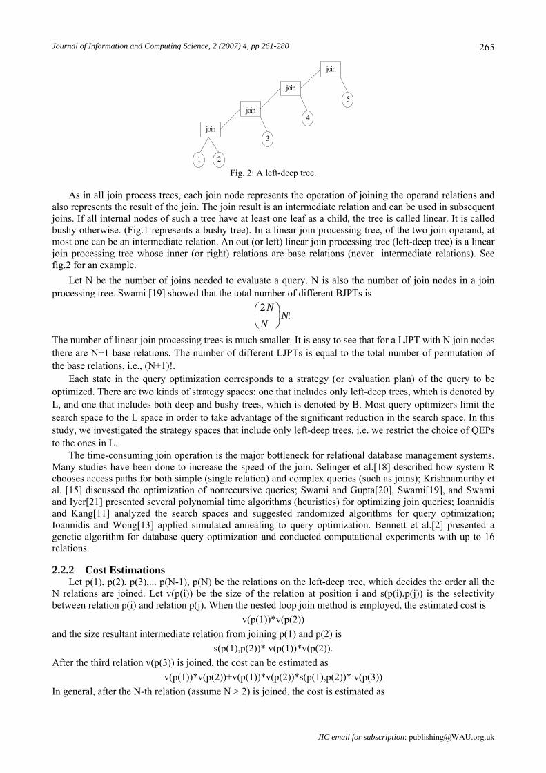
Fig. 2: A left-deep tree.
As in all join process trees, each join node represents the operation of joining the operand relations and also represents the result of the join. The join result is an intermediate relation and can be used in subsequent joins. If all internal nodes of such a tree have at least one leaf as a child, the tree is called linear. It is called bushy otherwise. (Fig.1 represents a bushy tree). In a linear join processing tree, of the two join operand, at most one can be an intermediate relation. An out (or left) linear join processing tree (left-deep tree) is a linear join processing tree whose inner (or right) relations are base relations (never intermediate relations). See fig.2 for an example.
Let N be the number of joins needed to evaluate a query. N is also the number of join nodes in a join processing tree. Swami [19] showed that the total number of different BJPTs is
2NN
N⎛⎝⎜
⎞⎠⎟ !
The number of linear join processing trees is much smaller. It is easy to see that for a LJPT with N join nodes there are N+1 base relations. The number of different LJPTs is equal to the total number of permutation of the base relations, i.e., (N+1)!.
Each state in the query optimization corresponds to a strategy (or evaluation plan) of the query to be optimized. There are two kinds of strategy spaces: one that includes only left-deep trees, which is denoted by L, and one that includes both deep and bushy trees, which is denoted by B. Most query optimizers limit the search space to the L space in order to take advantage of the significant reduction in the search space. In this study, we investigated the strategy spaces that include only left-deep trees, i.e. we restrict the choice of QEPs to the ones in L.
The time-consuming join operation is the major bottleneck for relational database management systems. Many studies have been done to increase the speed of the join. Selinger et al.[18] described how system R chooses access paths for both simple (single relation) and complex queries (such as joins); Krishnamurthy et al. [15] discussed the optimization of nonrecursive queries; Swami and Gupta[20], Swami[19], and Swami and Iyer[21] presented several polynomial time algorithms (heuristics) for optimizing join queries; Ioannidis and Kang[11] analyzed the search spaces and suggested randomized algorithms for query optimization; Ioannidis and Wong[13] applied simulated annealing to query optimization. Bennett et al.[2] presented a genetic algorithm for database query optimization and conducted computational experiments with up to 16 relations.
2.2.2 Cost Estimations Let p(1), p(2), p(3),... p(N-1), p(N) be the relations on the left-deep tree, which decides the order all the
N relations are joined. Let v(p(i)) be the size of the relation at position i and s(p(i),p(j)) is the selectivity between relation p(i) and relation p(j). When the nested loop join method is employed, the estimated cost is
v(p(1))*v(p(2)) and the size resultant intermediate relation from joining p(1) and p(2) is
s(p(1),p(2))* v(p(1))*v(p(2)). After the third relation v(p(3)) is joined, the cost can be estimated as
v(p(1))*v(p(2))+v(p(1))*v(p(2))*s(p(1),p(2))* v(p(3)) In general, after the N-th relation (assume N > 2) is joined, the cost is estimated as
JIC email for subscription: [email protected]

Z. Zhou: Using Heuristics and Genetic Algorithms for Large-scale Database Query Optimization 266
v p v p s j j v p jj
i
i
N
( ( ))* ( ( ))( ( , )* ( ( )))1 2 1 1 21
1
2
1
+ +=
−
=
−
∏∑ +
where we define v(p(n+1)) = v(p(1)). This cost function is the same as the cost function we develop for the open weighted cumulative
multiplication TSP problem (please refer to the appendix at the end of this paper), which indicates that the query optimization problem with nested looped joins can be interpreted as an open weighted cumulative multiplication TSP problem and thus is NP-hard. If other join methods are used, the cost function will be different. We observe that although the cost functions are different, dependent on the merger methods, the cost of C can be in the format of
f1(v(i),v(j)) + f2(V(i),v(j),s(i,j),v(l)) when relation (either base relation or intermediate relation) i is joined with relation j and then followed by the joining of relation l. The generic cost function will take the form of the summation of the products of sizes of the relations and selectivity at stages.
Although the cost estimate is somewhat crude, it is very general and represents a range of cost functions that take many major factors into consideration. We believe that if a heuristic works well for this cost model, it should be a viable algorithm for this class of cost functions also.
2.2.3 Cost Estimation for Distributed Databases In the previous subsection, we discussed the query optimization and cost estimation for centralized
systems. This is relevant to and necessary for understanding distributed query optimization because (1) a distributed query is translated into local queries, each of which is virtually processed in a centralized way, and (2) as has been done in the past, distributed query optimization techniques are often, if not always, extensions of the techniques developed and tested for centralized systems, and (3) centralized query optimization is much simpler in some sense compared to distributed query optimization, where the cost of communications makes it more complex and complicated. In other words, centralized query optimization is an important component of the distributed query optimization problem and also the first step of distributed query optimization. Several algorithms have been presented for distributed query optimization. Among them are: the reduction algorithm of distributed INGRES[5], System R* algorithm[18], SDD-1 algorithm[3], and the set of algorithms of Appers, Hevner, and Yao[1].
We can extend the cost model in the previous subsection to distributed query optimization, taking transmission cost into account. After the fragmented queries are completed in the local level, the results in each site can be considered as an intermediate relation. These intermediate relations need to be joined to produce the final answer to the original query. From this point of view, we are now faced a new query optimization problem in which the relations are residing in different places. Even if we still restrict our search to L space, the problem is more complex than the one discussed in the previous sections. First, the transmission cost should be considered since it is often a major, if not a dominating, component in the total cost function. Second, the search space becomes even larger. Suppose the relation (either base relation or intermediate relation) i is joined with relation j and followed by the joining of relation l. We now have two choices: either move the intermediate result from joining relations i and j to the site where relation l is located or transmit relation l to the site where relations i and j were joined. This site can be the site where relation i is located or relation j is located depending on the decision made on joining relations i and j. The total number of strategies in the space of left-deep tree for this step of distributed query optimization is thus (N+1)!*2N instead of (N+1)!, where N is the number of relations (i.e. the number of sites). Let D = (dlm ) be the matrix of the unit transmission cost from site m to site l. The transmission cost of relation i with size v(i) located at site i to site j is v(i)*dij. The cost functions in the previous section can thus be modified by adding the cost of transmission. The distributed query optimization problem at this step of distributed query processing is quite similar to the query optimization, or more specifically, the query ordering problem discussed in the previous section except that
(1) the transmission costs need to be added to the cost functions; and (2) in addition to the ordering of joins decided by (based on) the processing tree, the total costs are
usually different depending on which relation is transmitted to the other site; and (3) the cost of transmitting the final results to the place where the original query is issued should be
added to the total cost when the strategies are evaluated.
JIC email for contribution: [email protected]

Journal of Information and Computing Science, 2 (2007) 4, pp 261-280
267
Since the forms of the cost functions are quite similar, this extension should not be very difficult. The computational results from the local query optimization should also shed some light on the quality of solutions if modified algorithms are used for the distributed version of query optimization. Some simple heuristics may be used to simplify the distributed query optimization. For example, we may assume that an intermediate relation will always be transmitted to the other site or the relation with smaller size will always be transmitted and the permutation of the relations will then decide the joining process (including the order of joins and how the relations are moved). For example, we assume that an intermediate relation will always be transmitted to the other site; the total cost can be estimated as follows:
total cost = cost of joining + transmission cost + cost of transmitting the final results where
cost of joining = ∑∏−
=
−
=
+++1
2
1
1
)))2((*)1,(1))(2((*))1((N
i
i
j
jpvjjspvpv
as discussed above, and
transmission cost = ρ * { } d s j j v p ji ij
i
i
N
, ( , )* ( ( ))+
==
−
−∏∑ 111
1
1
where we define s(0,1) = 1 and ρ is a coefficient that makes the transmission cost comparable to the cost of joining operations.
cost of transmitting the final results = ρ * s j j v p jj
N
( , )* ( ( )−=∏ 1
1)
Since the cost of transmitting the final results to the initializing location is much less than the cost of transmitting intermediate relations or the cost of the joining operations. It may, in most cases, be ignored without much penalty.
3. Solution Methods The query optimization problem can be transformed to a join ordering problem which is a NP-hard
combinatorial optimization problem. So it is highly unlikely one could devise a polynomial algorithm to solve it efficiently. In the following, we describe several heuristics with which we will experiment on searching on the L spaces for query optimization. We will show how two of the algorithms, nearest neighbor and farthest insertion, used to solve traveling salesman problems, are adopted for the query optimization problem. We also briefly describe the genetic algorithm and show how to apply it to solve the query optimization problem
3.1. Order Construction Heuristics The algorithms discussed in this subsection are order construction procedures. Except random sampling,
they build on an approximate optimal order starting from some initial point(s) based on the selectivity matrix and the size of the relations. Random Sampling (RS)
The technique of random sampling is one of the simplest. One keeps generating new ‘random’ solutions (i.e. a permutations), remembering the lowest cost state visited. When the algorithm terminates (under the stopping criterion such as number of generations, the running time limits, etc.), the lowest cost solution encountered is output as the best solution found. Nearest Neighbor (NN)
NN algorithm is one of the most simpleminded and yet appealing greedy algorithms for constructing an order. It is simple to code and very efficient to perform. Starting from a random initial point, each run takes O(N2) operations. Since we can start from at most N initial points, the time complexity for nearest neighbor algorithms is O(N3). Because of the cumulative multiplication type of objective functions in query optimization, a greedy algorithm like nearest neighbor may be attractive and effective as well as efficient.
Nearest Neighbor Algorithm works as follows:
JIC email for subscription: [email protected]

Z. Zhou: Using Heuristics and Genetic Algorithms for Large-scale Database Query Optimization 268
step 1. Start with a partial order consisting of a single, arbitrarily (randomly) selected relation P1; step 2. Suppose the current partial order is P1, P2, P3, ..., Pk, k<n. Let Pk+1 be the relation which is not
currently on the order and closest to Pk, and add Pk+1 to the end of the (partial) order by connecting Pk and Pk+1;
step 3. Repeat step 2 until the current order contains all the relations. Farthest Insertion (FI)
Since the selection of the optimal ordering for a query is generally NP-complete, and thus computationally intractable, the actual objective of the query optimizer is to find a strategy close to optimal and, perhaps more important, to avoid the bad strategies. The farthest insertion algorithm may be a good candidate serving this kind of strategy. Although it may seem strange to see that farthest insertion chooses the locally worst point (farthest point) to link, rather than the best, there are reasons that this might not be a bad idea after all. The farthest points will be eventually connected to the order sooner or later. Putting the farthest points in first results in the establishment of the outline for the overall shape of the order. The order is then refined by adding in the remaining points that are close enough so that their addition has only minor effects on the overall order length. Empirical evidences show that farthest insertion is among the best heuristics for solving traveling salesman problems with Euclidean distance. Since our cost models of query optimization are much more complex due to the factors such as the sizes of the relation, selectivity, etc., it is not clear at all how well farthest insertion algorithm performs. Nevertheless, it is interesting and worthwhile to test the effectiveness of farthest insertion algorithm for query optimization.
Farthest insertion algorithm: step 1. Start with a partial order consisting of a single, arbitrarily chosen relation i; step 2. If the current partial order does not include all the relations, find the relation k which is farthest from the current partial order, i.e., choose relation k, not on order T, which maximizes min{sjk*vk: j is on T}, where vk is the size of relation k and sjk is the selectivity between relations j and k. step 3. Add k to the current order in the best place it fits:
case 1. If T consists of single relation i, then the new order T’ is the two-relation partial order consisting of the sequence {i,k};
case 2. If T consists of more than one relation, let {i, j} be the two relations of T that minimizes the objective function if k is inserted between these two relations and build the new order T’ by inserting relation k between relations i and j, i.e., obtain the new order {..., i, k, j, ...}.
3.2. Genetic Algorithms (GA) Since the query optimization problem is a difficult combinatorial optimization problem with complicated
objective functions, it is not easy to deal with by most ordinary techniques, either exact or heuristic. We thus choose to make use of another technique, the genetic algorithm, to search for solutions to the query optimization problem. Our major goal is not to outperform or to find better solutions than the other heuristic approaches, but to show that genetic algorithms may be very effectively applied to the query optimization problem with a very large number of relations and to describe in some detail how to accomplish it.
3.2.1. Genetic algorithm background In this subsection, we briefly describe the genetic algorithms. Genetic algorithms are a family of
computational models inspired by nature, or more specifically, by biological evolution. The concept of Genetic Algorithms was first presented formally by John Holland and is thoroughly described in many texts. Holland's work was based upon attempts to mimic in a computational environment the processes of natural selection proposed more than a century ago by Charles Darwin in his controversial work - ‘The Origin of the Species’ by means of natural selection.
A Genetic Algorithm generates a family of randomly generated solutions to the problem being investigated. Each of the solutions is evaluated to find out how fit it is, and a fitness value is assigned to each solution. At this point the solutions can be seen to be analogous to chromosomes in nature: a chromosome consists of a string of genes in evolution while a solution consists of a string of elements. The individuals are then given opportunities to ‘reproduce’ based on their fitness. Usually, pairs of solutions are selected for reproduction, with a bias towards the best solutions being chosen (in analogy of the concept of survival of the fittest). The chosen parents exchange parts of their genetic materials to produce a pair of new solutions. The purpose of this so-called 'Crossover' operator is to allow the best characteristics of ancestors (solutions) to combine in order to produce better off-
JIC email for contribution: [email protected]

Journal of Information and Computing Science, 2 (2007) 4, pp 261-280
269
springs (solutions) whose fitness is great than that of either parent. One of the most common operators applied is that of 'Mutation' as it can arise in nature and can make
striking changes to the features of an individual. Mutation is applied at random to genes (elements) in solutions. If the solution is represented as a string of bits, mutation changes a bit to the different value. For example, if a solution is represented as '01010010' and the third bit is randomly selected for mutation, the solution then becomes '01110010'.
Genetic Algorithms are widely applied to optimization problems, often run with and/or against other optimization methods, such as hill climbing techniques, simulated annealing, neural networks, etc. Genetic algorithms turned out to be viable and/or promising technique and have been accepted by more and more researchers. The main advantage of genetic algorithms over the more conventional methods is that the classic methods usually require a continuously differentiable function. A genetic algorithm, on the other hand, only requires that a solution can be represented as a list of genes (elements), which makes genetic algorithms very attractive. One of the key advantages of the genetic algorithms to search for solutions is that genetic algorithms do not rely upon specific knowledge of the problems on hand. They perform a purely non-heuristic search through the solution space and only the fitness function needs to apply information specific to the problem. They are so robust and flexible that they are applied to and work well in very complex systems, such as those with discontinuous, multi-modal, noise search spaces.
Genetic algorithms may be more suitable to complex problems than simple ones. Although they can be classified as probabilistic algorithms, they are very different from other random algorithms in the way that they combine the elements of directed and stochastic search. They tend to balance two objectives: exploiting the best solution(s) and exploring the search space. Unlike random search, which explores the search space but neglects the exploitation of the promising neighborhood (or regions) of the space, or hill climbing, which exploits the best solution for possible improvement but ignores exploration of the search space.
Another important property of genetic algorithms is that they usually maintain a pool (population) of potential solutions while almost all other methods process only a single point of the search space. This property has two important implications: first, it means the important characteristics of efficient parallelization (sometimes called implicit parallelism) which we do not exploit in this study; and second, the genetic algorithms provide not only the ‘best’ solution, but also a pool of good solutions that shed light on the effects of alternatives available. Further more, one can easily implement genetic algorithms such that multi-criteria are evaluated. This feature is extremely important nowadays since most, if not all organizations have many diverse and often conflicting objectives.
Because of their advantages or characteristics mentioned above, genetic algorithms are becoming a widely used and accepted technique for very difficult optimization problems, such as database design, query optimization, travelling salesman problem, among many others. Genetic algorithm components
The structure of a genetic algorithm is shown as follows: PSEUDO CODE Algorithm Genetic Algorithm (GA) Input: Output: begin // start with an initial time t := 0; // initialize a usually random population of individuals initpopulation P (t); // evaluate fitness of all initial individuals of population evaluate P (t); // test for termination criterion (time, fitness, etc.) while not done do begin // increase the time counter
JIC email for subscription: [email protected]

Z. Zhou: Using Heuristics and Genetic Algorithms for Large-scale Database Query Optimization 270
t := t + 1; // select a sub-population for offspring production P' := selectparents P (t); // recombine the "genes" of selected parents recombine P' (t); // perturb the mated population statistically mutate P' (t); // evaluate it's new fitness evaluate P' (t); // select the survivors from actual fitness P := survive P,P' (t); end-do end. {GA} The major aspects of a genetic algorithm are described below:
Representation (coding) The first and perhaps the most important step in applying a genetic algorithm to a problem is to devise a
suitable coding (representation) for the problem. The potential solution is represented as a finite-length string over a finite alphabet. These strings (often referred to as genes) are joined together to form another string of values (known as chromosomes). Many applications today use a string of binary digits to represent chromosome (solution). For instance, if we want to minimize a function of two variables, f(x,y), we might represent each variable by a 8-bit binary number (that is suitably scaled). The resultant chromosome would therefore consist of two genes, and contain 16 binary digits. However, the values on the chromosome should be able to be arranged and interpreted as needed. For example, the chromosome may represent integers, discretized real numbers, as well as Boolean values. The fitness function
It is important that a suitable fitness function be devised. The fitness function will interpret the chromosome and evaluate the chromosome’s fitness (usually a single numerical value) that is supposed to be proportional to the ‘ability’ or ‘utility’ of the individual which the chromosome represents. The fitness function needs to be defined over the set of possible chromosomes. Since the fitness function must accurately measure the desirability of the features represented by the chromosome and the large number of times the function will be called during the execution of the genetic algorithm, the definition of this function is crucial and should make the evaluation as efficient as possible. Obviously, the definition of the fitness function is problem dependent. For function optimization problems, the fitness function should be the functions to be optimized. For many other problems, there may be other performance measures we want to optimize. Reproduction
The reproduction process includes the selection, crossover (mating), and mutation of the chromosomes. Selection
Individuals are selected from the population and then recombined, producing off-springs (in the new generation). Parents are randomly chosen from the whole population using a scheme that favors the more fit individuals: fitter individuals may be selected more often than those less fit. Crossover
Crossover (usually) takes two individuals, and cuts their chromosome strings at some randomly chosen point. The ‘tail’ segments of the two strings are then exchanged to generate two new full length chromosomes, each of which inherits some genes (characteristics) from each parent. Crossover is not usually applied to all individuals and individuals are randomly chosen for crossover. If crossover is not applied, off-springs are produced simply by duplicating the parents through the selection process and the individual hence has a chance to pass on its genetic materials without the disruption of crossover. It is more desirable if off-springs from crossover are fitter than their parents. However, it is quite possible that crossover generates off-springs of low fit. These low fit individuals will be less likely to be selected for reproduction in the next generation. The following is an example of crossover and mutation:
JIC email for contribution: [email protected]

Journal of Information and Computing Science, 2 (2007) 4, pp 261-280
271
before crossover 10101010 111|10000 11001100 110|01100 after crossover 10101010 11101100 11001100 11010000 which may be mutated into: 10111010 11101000 11001100 01010000
Mutation After crossover is completed, mutation is applied to each offspring individually. Mutation alters each gene
with a typically small probability. For the binary alphabet cases, this is done simply by changing the bit value from 1 to 0 or vice versa. Fig.4 shows that genes of the two chromosomes are mutated at two and one position, respectively.
The reproduction process actually manipulates the individual chromosomes and must, therefore, be decided with the underlying encoding of the chromosomes in mind. When defining reproduction operators like crossover, which performs a ‘crossover’ or mating of two chromosomes, care must be taken such that the mixing of gene values will produce viable off-springs. Otherwise, repairing (with cost) will have to be done to fix the nonviable off-springs. The same is true for mutation.
Crossover is considered to be more important than mutation for exploring the search space rapidly. Mutation provides a small amount of random search and is used to ensure that selection and crossover do not lose potentially useful genetic materials. In other words, it is supposed to help ensure that no point in the search space would have no chance to be examined. Control parameters of a genetic algorithm
There are several other control parameters that govern the genetic algorithm search process. The major ones are:
Number of generations specifies how many times the population will be replaced through reproduction. Population size determines the number of individuals (chromosomes) available for use during the search. If
the size is too big, the genetic algorithm will spend unnecessarily long time evaluating chromosomes. If there is too few genetic material, the search may have no chance to adequately cover the search space.
Crossover rate is the probability of crossover (mating) between two chromosomes. Mutation rate specifies the probability that values of genes of a newly created (or selected) off-springs will
be randomly changed. Since our major purpose of this part of the dissertation is to devise algorithms and compare their
effectiveness to solve the query optimization problem, not find the best set of parameter values for a specific or a group of instances, we only discuss and test the parameters briefly.
3.2.2. Applying a genetic algorithm to query optimization Our approach to the query optimization problem uses a genetic algorithm to search through the space of
left-deep trees over the set of relations. As we mentioned before, the search space is a set of permutation of N relations. Any single permutation of N relations yields a solution (which determines the join ordering). The optimal solution is the permutation which yields the minimum cost of the order among the N! possible ones. Representation
Unlike many other applications of genetic algorithms, it is not clear how the chromosomes should be represented in query optimization problem. We have two basic choices: (1) leave a chromosome to be an integer vector (e.g. [1 2 3... N-1 N]), or (2) transform it into a binary string. In a binary representation of N relation query optimization problem, each relation should be coded as a string of ┌ log2 N ┐ bits. A chromosome is thus a string of N*┌ log2 N ┐ bits. A problem arises: some sequences of a string of┌ log2 N ┐bits maybe do not correspond to any relation and thus the chromosomes do not represent a solution which
JIC email for subscription: [email protected]

Z. Zhou: Using Heuristics and Genetic Algorithms for Large-scale Database Query Optimization 272
should be a permutation of N relations. In addition, a mutation or crossover may produce a sequence that is not a permutation. For instance, a number i may appear twice while a number j is missing from the sequence. Obviously, some sort of ‘repair algorithm’ is needed to fix a chromosome if binary representation is used.
The alternative integer vector representation may be more straightforward. However, cares have to be taken to avoid illegal sequences resulted from crossover and mutation. Instead of using ‘repair’ mechanism, we can incorporate the knowledge of the query optimization problem into some of the reproduction operators to avoid illegal chromosomes.
The query optimization problem is similar to the TSP problem in the sense that a permutation with minimum cost is searched. We again can adopt some of the ideas developed for solving TSP using genetic algorithm. Several vector representations for TSP have been presented during the past few years. Among them, adjacency representation, ordinal representation, path representation are commonly used. We choose to use path representation in our study. The path representation is employed in this research mainly because it is perhaps the most natural and straightforward representation of a permutation (tour, order). For instance, a tour
2-7-4-10-6-8-1-9-7-5-3 is represented as
(2 7 4 10 6 8 1 9 7 5 3). Path representation has its own ‘genetic’ operators. There have been three crossover operators
considered connected with TSP: cycle (CX), order (OX), partially mapped (PMX). In this study, the order crossover (OX) is used. OX works as follow:
Off-springs are generated by choosing a subsequence of a tour from one parent and preserving the relative order of cities from the other parent. For instance, the two parents (with two cutting points indicated by ‘|’) are as follows:
parent 1: ( 1 3 | 5 7 9 10 | 2 8 6 4 ) parent 2: ( 3 8 | 2 1 6 9 | 4 10 7 5 ) First, the sub-tours between the cutting points are preserved in the off-springs: off-spring 1: ( x x | 5 7 9 10 | x x x x ) off-spring 2: ( x x | 2 1 6 9 | x x x x ) Second, starting from the second cutting point of one parent, the cities from the other parent are copied
in the same order, deleting the cities already presented. The sequence cities in the second parent (starting from the second cutting point) is
4-10-7-5-3-8-2-1-6-9 after omitting cities 10, 7, 5, 9, which are already in the first offspring, we have
4-3-8-2-1-6 Placing the segment above in the first offspring (starting from the second cutting point) results in the
following new tour: off-spring 1: ( 1 6 |5 7 9 10 | 4 3 8 2 ) By the same procedure, we get the other offspring: off-spring 2: ( 7 10 | 2 1 6 9 | 8 4 3 5 ) Because some parents may generate more than one offspring in the selection process, two identical
individuals may be chosen for the crossover process. We modify Davis’ procedure so that two different off-springs will be generated after crossover even if the two parents are identical. When we place the segment obtained from parent 1 into offspring 2, we start from the beginning of the tour, in stead of starting from the second cutting point. So we actually get:
off-spring 1: ( 1 6 | 5 7 9 10 | 4 3 8 2 ) off-spring 2: ( 8 4 | 2 1 6 9 | 3 5 7 10 )
Mutation Mutation is a unary operator that supplements recombination operators. In this study, we use the
reciprocal exchange mutation that swaps the number at position i and the number at position at i+1, i<N. The number at position N is switched with the number at position 1. This simple mutation guarantees that the
JIC email for contribution: [email protected]

Journal of Information and Computing Science, 2 (2007) 4, pp 261-280
273
resulting offspring is a legal permutation and no repairing process is required. Selection
In some application of genetic algorithm, the choice of evaluation function is the hardest task. This is not the case in query optimization. Although the evaluation functions can be very complex and expensive to compute, they have very clear definition and meaning. They also indicate the fitness of individuals accurately. In most genetic algorithm applications today, the selection is based on the relative fitness of the individuals. For example, a chromosome is selected based on the ratio of the individual fitness over the total fitness of the whole population. While this method is reasonable and works very well in many applications, it might not be very suitable for our purpose. In query optimization, the fitness of individuals in a population vary considerably (we can see two individuals with fitness difference larger than 10100 for query optimization problem of 100 relations in our computational experiments). If selection is based on the relative fitness of the individuals, some chromosomes will have virtually no chance to produce off-springs while others may generate many. This tends to result in the premature convergence of the genetic algorithms and the search space will not be adequately searched. To avoid this problem, we suggest the following scaling scheme: sort the chromosome in descending order based on their objective function values, and assign the best individual the fitness value N, the second best individual N-1, and so on, i.e.
order 1 2 3 ... N-1 N fitness N N-1 N-2 ... 2 1 prob. N/T (N-1)/T (N-2)/T ... 2/T 1/T where prob. is the probability that an individual be selected to produce offspring and T is the total (scaled)
fitness value, i.e. T = (N+1)*N/2.
4. Computational Experiments In order to find how effectively and/or efficiently we can solve query optimization problems using the
algorithms discussed above and to observe the advantages (characteristics) and/or disadvantages (limitations, pitfalls) of the algorithms over each other, some computational experiments were conducted. We tested the order construction algorithms, including random sampling, nearest neighbor, farthest insertion, and genetic algorithms. To evaluate the quality of the solutions and for completeness, we employed exhaustive search (ES) and found the optimal solutions for all the 10 instances when the number of relations (N) equals 10.
Table 1. Objective values for ES, RS, GA, NN and FI (N=10)
ES
RS
1000
RS
10000
RS
100000
GA
100
GA
1000
GA
10000 NN FI
1 979.305 8289.49 8289.49 7440.83 2.40957e4 1102.47 979.305** 979.305** 5.45368e4
2 3.53257e6 4.68525e7 2.09419e7 1.24402e7 1.54059e7 3.53257e6 3.53257e6** 1.53646e7 2.39595e7
3 1067.2 1067.2** 1067.2** 1067.2** 1067.2** 1067.2** 1067.2** 1104 1104
4 2.01109e6 1.56254e7 1.56254e7 4.21349e6 8.26994e6 2.53600e6 2.01109e6** 2.23292e6 9.27126e6
5 2.46814e4 5.99346e5 1.21652e5 3.99147e4 4.60147e5 2.46814e4 2.46814e4** 4.22192e4 4.11674e4
6 7.36926e6 5.42960e7 5.42960e7 3.41948e7 3.07793e7 1.40024e7 7.36926e6** 7.36926e6** 2.97086e7
7 3.15617e6 6.08337e7 2.67921e7 8.33802e6 1.02759e7 3.15617e6 3.15617e6** 7.29951e6 1.17995e7
8 5.98128e4 3.38374e6 7.79669e5 2.14128e5 1.67803e6 8.81375e4 6.80085e4* 8.55703e4 5.15008e5
9 1823.96 8.99795e4 2.72882e4 6130.73 6.35142e4 2567.62 1823.96** 1.56854e4 2.21095e4
10 9.51665e4 8.16366e5 6.59506e5 2.34326e5 3.25035e5 1.31308e5 9.51665e4** 5.10088e5 8.35484e5
JIC email for subscription: [email protected]

Z. Zhou: Using Heuristics and Genetic Algorithms for Large-scale Database Query Optimization 274
Table 2. Objective values for RS, GA, NN and FI (N=20)
RS
1000
RS
10000
RS
100000
GA
100
GA
1000
GA
10000
NN FI
1 32* 32* 32* 32* 32* 32* 32* 32*
2 316.02 133.44 88.2483 416 38.688* 38.688* 38.688 80.1723
3 578* 578* 578* 578* 578* 578* 578* 578*
4 288 89.6* 89.6* 89.6* 89.6* 89.6* 156.672 288
5 6.25606e12 4.60251e11 3.55383e10 1.36672e9 4.04049e7 3.86621e5 6.68207e4* 2.05828e8
6 8.34726e14 1.07772e13 1.07772e13 3.39608e10 1.18984e9 7.96105e8* 6.92266e9 1.37625e11
7 14* 14* 14* 14* 14* 14* 14* 14*
8 4.20768e12 4.20768e12 7.74673e8 3.36760e9 5.91610e5 2.36128e5 1.65480e4* 3.51884e5
9 344.724 285.12 77.8752* 1645 486.45 210.427 77.8752* 726
10 1295 1295 894.738 1295 1295 317.421* 1295 1295
Table 3. Objective values for RS, GA, NN and FI (N=60)
RS
1000
RS
10000
RS
100000
GA
100
GA
1000
GA
10000
NN FI
1 72 60 17.2 320 31.44 19.2879 8.244* 9.70813
2 80 4* 4* 81 4* 4* 4* 4*
3 256 46.4 45.28 64 2.64* 2.64* 2.64* 24.423
4 210 168 41.04 190 190 39.28 14.2215* 31.9031
5 36 36 32.97* 722 48.33 36 36 36
6 16 16 8.7132 456 27.81 3.36065* 3.6216 13.2391
7 6* 6* 6* 107.38 84 6* 6* 6*
8 18 12.2948 7.08 45 45 3.73408* 7.08 18
9 35 35 31.55 96 14.8358 4.42418* 14.32 13.8071
10 63* 63* 63* 140 140 63* 63* 63*
Table 4. Objective values for RS, GA, NN and FI (N=100)
RS
1000
RS
10000
RS
100000
GA
100
GA
1000
GA
10000
NN FI
1 60 14.16 14.16 16 15.04 12.72 6.96192* 16
2 42 12 12 2816.53 646 4.3296* 4.3296* 12
3 120 11* 11* 220 125 11* 11* 11*
4 108 22 12.32* 228 48 21.2256 22 12.0035*
5 39 17 17 180 180 12.12* 12.12* 17
6 9 9 9 46 20.56 2.776* 3.9 3.05688
7 58.5 16 1.64* 16 16 1.64* 5.2 3.3644
8 20 10 6.50086 1569.24 56 5.52296 3.3* 6.49555
9 69 34 14.2284 910 34 5.6024 3.71* 14.2622
10 30 28 19.7 252 252 8.44* 9.45 28
JIC email for contribution: [email protected]

Journal of Information and Computing Science, 2 (2007) 4, pp 261-280
275
Table 5. Objective values for RS, GA, NN and FI (N=140)
RS
1000
RS
10000
RS
100000
GA
100
GA
1000
GA
10000
NN FI
1 68 8 8 49 14.24 5.7* 6.1824 8
2 54 18 5* 509.133 88 5* 5* 5*
3 12 12 12 3848.46 12 12 9.84 5.12*
4 190.243 11 11 347.494 14 9.93 7.77* 11
5 108 21 21 108 108 6.7488* 7.74 6.98549
6 5 5 4.12 163.2 21 4.6 5 1.17791*
7 126 12 4.9 119 14.393 4.24* 5.43 5.43768
8 46 18 11.52 39.48 39.48 10.9406 3 2.46*
9 20 16 2.38 269.62 27.2 1.64512* 5.28 2.51734
10 132 14 1.84 14 14 1.08333* 6 4.83948
In the experiments we conducted, we used 10 different queries for each N, where N is the number of relations, N = 10, 20, 60, 100, 140. This gave a total of 50 different queries. The experiments were performed using the main memory cost model described in Section 2. Since the cost models are quite similar, we expect that solutions at about the same level of quality can be obtained if other models are employed. All the 50 queries are randomly generated. The size of each relation, vi, is randomly generated and falls in the range [1,50] and the selectivity, sij, between relations i and j is randomly generated and takes the values between 0 and 1, i.e. vi ∈ [1,50] and sij ∈ [0,1]. When N = 10, we tested the following algorithms: exhaustive search (ES), random sampling (RS), genetic algorithm (GA), nearest neighbor (NN), and farthest insertion (FI). For the exhaustive search, we generated and evaluated all the 10! = 3,628,800 QEPs and found out the solution with lowest objective value. For nearest neighbor (NN) and farthest insertion (FI), we started the algorithms with 10 different initial points. In other words, the algorithms were run 10 times with different initial points. For random sampling (RS), we employed three different number of sample sizes (which is the number of random permutations generated): 1000, 10,000, and 100,000. For genetic algorithm, we used the following set of parameters:
Parameters Values used Population Size 10 chromosomes Number of Generations 100, or 1000, or 10,000 Crossover Percentage 0.2 percent Mutation Percentage 0.05 percent To facilitate comparison and analysis, the computational results are summarized in Tables 1-5. The numerical numbers under GA are the number of generations run before the processes stopped while the numbers under RS are the number of sample permutations (solutions) generated. ** indicates that an optimal solution value for the problem and * indicates the best solution (not necessarily optimal) obtained for a problem. We found the following preliminary results:
• GA outperforms RS in terms of solution quality (effectiveness); • NN and FI generate comparable, if not better, results than RS with large sample sizes (say, 100,000),
and both are viable alternatives for solving the query optimization problems; • The nearest neighbor algorithm performs better than the farthest insertion algorithm in terms of
effectiveness when N is small. As N increases, the latter does better than the former. Theoretically, it is easy to see that NN is more efficient (fast) that FI. In our computational experiments, NN is usually one order faster than FI;
• Overall, GA outperforms all other algorithms (ES not included) in terms of solution quality. • Since we use N initial points for NN and FI, there is no way that we can improve the results for NN
and FI. So NN and FI have disadvantages compared to GA. In GA, it is possible to get better
JIC email for subscription: [email protected]

Z. Zhou: Using Heuristics and Genetic Algorithms for Large-scale Database Query Optimization 276
solutions by using more appropriate parameters (e.g., mutation rate, crossover rate, etc.) or increase the number of generations to be run;
• GA is least efficient among the algorithms tested (ES not included); • When N is small, FI, especially NN, generates good solutions. However, as N increases, the quality
of solutions produced by NN and FI decreases. Table 6. Objective values for ES, RS, GA, NN and FI (N=10)
ES RS
1000
RS
10000
RS
100000
GA
100
GA
1000
GA
10000
NN FI
1 979.305 8289.49 8289.49 7440.83 4.89973e4 8612.35 979.305** 979.305** 5.45368e4
2 3.53257e6 4.68525e7 2.09419e7 1.24402e7 1.26501e7 5.46343e6 3.53257e6** 1.53646e7 2.39595e7
3 1067.2 1067.2 1067.2 1067.2 1067.2 1067.2 1067.2** 1104 1104
4 2.01109e6 1.56254e7 1.56254e7 4.21349e6 1.32868e7 2.01109e6 2.01109e6** 2.23292e6 9.27126e6
5 2.46814e4 5.99346e5 1.21652e5 3.99147e4 1.15455e5 4.88734e4 2.46814e4** 4.22192e4 4.11674e4
6 7.36926e6 5.42960e7 5.42960e7 3.41948e7 7.54373e7 7.36926e6** 7.36926e6** 7.36926e6 2.97086e7
7 3.15617e6 6.08337e7 2.67921e7 8.33802e6 3.15617e6** 3.15617e6** 3.15617e6** 7.29951e6 1.17995e7
8 5.98128e4 3.38374e6 7.79669e5 2.14128e5 6.91591e6 5.98128e4** 5.98128e4** 8.55703e4 5.15008e5
9 1823.96 8.99795e4 2.72882e4 6130.73 5021.63 5021.63 1823.96** 1.56854e4 2.21095e4
10 9.51665e4 8.16366e5 6.59506e5 2.34326e5 2.48905e5 1.48526e5 9.83896e4* 5.10088e5 8.35484e5
population size: 5; crossover rate: 0.4; mutation rate: 0.05
Table 7. Objective values for RS, GA, NN and FI (N=20)
RS
1000
RS
10000
RS
100000
GA
100
GA
1000
GA
10000
NN FI
1 32* 32* 32* 32* 32* 32* 32* 32*
2 316.02 133.44 88.2483 118.414 38.688* 38.688* 38.688* 80.1723
3 578* 578* 578* 578* 578* 578* 578* 578*
4 288 89.6* 89.6* 89.6* 89.6* 89.6* 156.672 288
5 6.25606e12 4.60251e11 3.55383e10 1.75637e8 1.67114e7 1.63765e5 6.68207e4* 2.05828e8
6 8.34726e14 1.07772e13 1.07772e13 4.70439e10 2.16493e10 5.59000e8* 6.92266e9 1.37625e11
7 14* 14* 14* 14* 14* 14* 14* 14*
8 4.20768e12 4.20768e12 7.74673e8 1.00870e8 1.14899e5 3313.4* 1.65480e4 3.51884e5
9 344.724 285.12 77.8752* 222.309 222.309 77.8752* 77.872* 726
10 1295 1295 894.738 1295 1295 317.421* 1295 1295
population size: 10; crossover rate: 0.4; mutation rate: 0.05
Table 8. Objective values for RS, GA, NN and FI (N=60)
RS 1000 RS 10000 RS 100000 GA 100 GA 1000 GA 10000 NN FI
1 72 60 17.2 27.82 27.82 10.011 8.244* 9.70813
2 80 4* 4* 4* 4* 4* 4* 4*
3 256 46.4 45.28 64 64 2.64* 2.64* 24.423
4 210 168 41.04 210 12.736* 12.736* 14.2215 31.9031
5 36 36 32.97* 133 36 36 36 36
6 16 16 8.7132 33 8.4 3.6216* 3.6216* 13.2391
7 6* 6* 6* 90 6* 6* 6* 6*
8 18 12.2948 7.08 180 3.1328 1.90851* 7.08 18
9 35 35 31.55 78.4 23.75 9.7* 14.32 13.8071
10 63* 63* 63* 816 63* 63* 63* 63*
population size: 20; crossover rate: 0.4; mutation rate: 0.05
JIC email for contribution: [email protected]
Journal of Information and Computing Science, 2 (2007) 4, pp 261-280
277
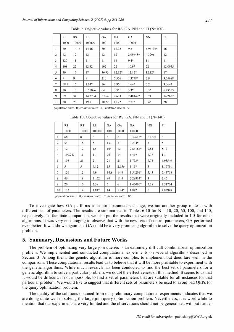
Table 9. Objective values for RS, GA, NN and FI (N=100)
RS
1000
RS
10000
RS
100000
GA
100
GA
1000
GA
10000
NN FI
1 60 14.16 14.16 60 12.72 9.2 6.96192* 16
2 42 12 12 12 12 2.99648* 4.3296 12
3 120 11 11 11 11 9.4* 11 11
4 108 22 12.32 102 22 10.9* 22 12.0035
5 39 17 17 36.93 12.12* 12.12* 12.12* 17
6 9 9 9 210 7.556 1.3778* 3.9 3.05688
7 58.5 16 1.64* 16 2.96 1.64* 5.2 3.3644
8 20 10 6.50086 64 3.3* 3.3* 3.3* 6.49555
9 69 34 14.2284 5.864 2.683 2.48447* 3.71 14.2622
10 30 28 19.7 10.22 10.22 7.77* 9.45 28
population size: 60; crossover rate: 0.4; mutation rate: 0.05
Table 10 . Objective values for RS, GA, NN and FI (N=140)
RS
1000
RS
10000
RS
100000
GA
100
GA
1000
GA
10000
NN FI
1 68 8 8 8 8 3.32615* 6.1824 8
2 54 18 5 133 5 3.234* 5 5
3 12 12 12 104 12 2.86162* 9.84 5.12
4 190.243 11 11 76 14 6.46* 7.77 11
5 108 21 21 21 21 5.793* 7.74 6.98549
6 5 5 4.12 15 2.656 1.15* 5 1.17791
7 126 12 4.9 14.8 14.8 1.54201* 5.43 5.43768
8 46 18 11.52 90 11.4 2.28914* 3 2.46
9 20 16 2.38 6 6 1.47080* 5.28 2.51734
10 132 14 1.84* 14 1.84* 1.84* 6 4.83948
population size: 100; crossover rate: 0.2; mutation rate: 0.05
To investigate how GA performs as control parameters change, we ran another group of tests with different sets of parameters. The results are summarized in Tables 6-10 for N = 10, 20, 60, 100, and 140, respectively. To facilitate comparison, we also put the results that were originally included in 1-5 for other algorithms. It was very encouraging to observe that with the new sets of control parameters, GA performed even better. It was shown again that GA could be a very promising algorithm to solve the query optimization problem.
5. Summary, Discussions and Future Works The problem of optimizing very large join queries is an extremely difficult combinatorial optimization
problem. We implemented and conducted computational experiments on several algorithms described in Section 3. Among them, the genetic algorithm is more complex to implement but does fare well in the comparisons. These computational results lead us to believe that it will be more profitable to experiment with the genetic algorithms. While much research has been conducted to find the best set of parameters for a genetic algorithm to solve a particular problem, we doubt the effectiveness of this method. It seems to us that it would be difficult, if not impossible, to find a set of parameters that are suitable for all instances for that particular problem. We would like to suggest that different sets of parameters be used to avoid bad QEPs for the query optimization problem.
The quality of the solutions obtained from our preliminary computational experiments indicates that we are doing quite well in solving the large join query optimization problem. Nevertheless, it is worthwhile to mention that our experiments are very limited and the observations should not be generalized without further
JIC email for subscription: [email protected]

Z. Zhou: Using Heuristics and Genetic Algorithms for Large-scale Database Query Optimization 278
investigation. GA and other heuristics have their own advantages and disadvantages. For some complex, large scale NP-hard problems like query optimization, GA may be a viable technique and is preferred because of its robustness and flexibility and its capability to exploit and explore the search spaces.
It is anticipated that the models for query optimization in distributed database systems and solution techniques developed for these models may be of practical, as well as theoretical use. Nevertheless, much more needs to be done to solve the distributed database design problems if the potential benefits of distributed database systems are to be achieved. We have shown the complexity of query optimization problems in large scale distributed database systems. Two stage methods (composite procedures) that apply the order construction procedures to begin with and the order improvement procedures next have the potentials to generate better results. First, we note that heuristics may find a solution that is not even a local optimal point. Some instances might cause a heuristic to break down. So it is in general useful (or even necessary) to use some local improvement procedures (like hill climbing, edge exchange, etc.) to obtain better solutions after an order construction procedure is completed. Heuristics, including the ones we discussed above, are not very expensive in terms of computation time. So it is also feasible to combine them with some other local improvement procedures in order to find better, local optimal solution(s). For optimization problems such as query optimization, we may be better off to enhance the GA algorithm. Since GA randomly searches some point in the solution space, it may end up with a point which is even not the local optimal point. We suggest that for optimization problems in general and for query optimization in particular, a post processing procedure be added to the GA. More specifically, we suggest that some techniques such as HCA or other local improvement procedures are used to find the local optimal points after the GA procedure is terminated.
For query optimization, a major challenge is to explore the space of bushy trees. The problem will become even more complex, but the benefits in terms of cost reduction can be significant. In addition, some relaxation or greedy heuristics, such as nearest merge, assignment problem, spanning tree, etc. that could be particularly suitable for this kind of search space might be used and possibly generate high quality solutions.
Our cost models are mainly for memory resident databases. While it is a reasonable assumption and will become more relevant, we understand that this assumption may not hold in some cases. It is of interest to see how well the heuristics and genetic algorithm we developed will perform under these circumstances.
Other objective functions also need to be taken into consideration. While we expect that algorithms including nearest neighbor, farthest insertion, genetic algorithms will be effective, we will try to modify the problem by changing the objective from minimizing total cost to other ones, such as minimizing response time. We will test whether the algorithms will be able to adapt to major changes in problem specification and continue to produce excellent results.
Other solution methods that have been shown to be very effective for TSP problems should also be tested for solving query optimization problems. Order construction procedures, such as nearest merge algorithms, nearest addition algorithms, cheapest insertion algorithms, arbitrary insertion, etc., may also turn out to be very good techniques for query optimization also. Local order improvement procedures, such as ones similar to variable r-opt for TSP need to be tested too
6. Appendix: The Traveling salesman problem and its variants The travailing salesman problem (TSP) is probably one of the most studied problems in combinatorial
optimization. In this appendix, we present several new variants of the classic traveling salesman problem and discuss their time complexity, which will, hopefully, lead to a better understanding the query optimization models we introduce in this paper. The Classical TSP Problem The statement of the traveling salesman problem is very simple: a traveling salesman must visit each and every city in his territory exactly once and then return to the starting city. Given the cost of travel between all pairs of cities, how should the traveling salesman plan his itinerary so that the total cost of his tour is minimum? More formally, TSP is defined as follows: INSTANCE: Integer n>2 and n*n matrix C = (cij), where each cij is a nonnegative integer.
QUESTION: Which cyclic permutationπ of the integers from 1 to n minimizing ? ci i
i
n
π ( )
=∑
1
JIC email for contribution: [email protected]

Journal of Information and Computing Science, 2 (2007) 4, pp 261-280
279
If the salesman can start his tour in any city but does not have to return to the first city in the end, the TSP is referred to as Open TSP (OTSP) or Wandering Salesman Problem (WSP). Multiplication TSP (MTSP)
If we define the objective function as the product of the costs of the edges in the tour, we get a new type of TSP problem which we will refer to as multiplication TSP. INSTANCE: Integer n>2 and n*n matrix C = (cij) , where each cij is a nonnegative integer.
QUESTION: Which cyclic permutationπ of the integers from 1 to n minimizing ? ci i
i
n
π ( )
=∏
1
Proposition 1: The multiplication TSP (MTSP) is NP-hard. Cumulative Multiplication TSP (CMTSP) INSTANCE: Integer n>2 and n*n matrix C = (cij), where each cij is a nonnegative integer.
QUESTION: Which cyclic permutationπ of the integers from 1 to n minimizing ? ci ii
n
i
n
π ( )==∏∑
11
Proposition 2: The cumulative multiplication TSP (CMTSP) is NP-hard. Weighted Cumulative Multiplication TSP (WCMTSP)
Now let us assume that there is a weight associated with each city (node). We define the objective function as the sum of the weighted products of the costs of the edges in all the sub-tours from the 1-st city to the 2-nd city, the 1-st city to the 3-rd city, …, the 1-st city to the current city, we get yet another new variant of the TSP problem (we call weighted cumulative multiplication TSP or cumulative multiplication TSP with node weight).
INSTANCE. Integer n>2, a vector of nonnegative integers, S = (si), and n*n matrix C = (cij), where each cij is a nonnegative integer.
QUESTION. Which cyclic permutation π of the integers from 1 to n minimizing
s s c j j s jj
i
i
n
( ( ))* ( ( ))( ( ( , )* ( ( ))))π π π1 2 1 1 212
1
+ +==
−
∏∑ + where we define s(π(n+1)) = s(π(1)).
Proposition 3: The weighted cumulative multiplication TSP (WCMTSP) is NP-hard. In the same way as we treated the classical TSP problem, we can also define the open versions (denoted as OMTSP, OCMTSP, and OWCMTSP, respectively) of MTSP, CMTSP, and WCMTSP by requiring open tours instead of close tours.
In order to show the time complexity of open versions of these variants of the classical traveling salesman problem, we need to introduce another problem which is well known to be NP-hard, Hamiltonian path problem. Hamiltonian Path
Hamiltonian cycle in a graph is a cycle (with n edges) passing all the vertices of this graph; a graph is said to be Hamiltonian if it has at least one Hamiltonian cycle. Hamiltonian path is a path (rather than a cycle and thus having n-1 edges) passing all the vertices of the graph. Both Hamiltonian cycle and Hamiltonian path are proved to be NP-hard [6]. Proposition 4: OMTSP, OCMTSP, and OWCMTSP are NP-hard. Proof: In the following we show only that OWCMTSP is NP-hard as stated in proposition 4 since the result will be used in the next subsection. The same arguments can be easily extended to OMTSP and OCMTSP to prove their NP-completeness.
We will make use of the result related to the Hamiltonian path problem. First, it is obvious that OCMTSP ∈ NP. Second, the Hamiltonian path problem can be polynomially transformed into an OCMTSP problem. Given any graph G = (V, E), we construct an instance of the |V|-city OCMTSP by letting cij = 1 if [vi, vj] ∈ E, and 2 otherwise. Let s(i) = 1 for all nodes. It is not difficult to see that there is a tour with objective value of |V|-1 if and only if there exists a Hamiltonian path in G.
JIC email for subscription: [email protected]

Z. Zhou: Using Heuristics and Genetic Algorithms for Large-scale Database Query Optimization 7. References
JIC email for contribution: [email protected]
280
[1] P.M.G. Apers, A.R. Hevner and S.B.Yao. Optimization algorithms for distributed queries. IEEE Transactions on Software Engineering, 1983, 9(1): 57-68.
[2] K. Bennett, M.C. Ferris and Y.E. Ioannidis. A genetic algorithm for database query optimization. In: R. Belew and L. Booker (eds.). Proceedings of the 4th International Conference on Genetic Algorithms. Los Altos, CA: Morgan Kaufmann Publishers, 1991, 400-407.
[3] P.A.Bernstein, N. Goodman, E. Wong, C.L. Reeve and J.B. Rothnie. Query processing in a system for distributed databases (SDD-1), ACM Transaction on Database Systems, 1981, 6(4): 602-625.
[4] L.Davis. Applying adaptive algorithms to epistatic domains. Proceedings of the International Joint Conference on Artificial Intelligence, 1985, 162-164.
[5] R. Epstein, M. Stonebraker and E. Wong. Query processing in a distributed relational database system. In: Proceedings of the ACM SIGMOD International Conference on Management of Data (Austin, Texas), 1978.
[6] M.R. Garey and D.S. Johnson. Computers and Intractability: A Guide to the Theory of NP-Completeness. W. H. Freeman, 1979.
[7] G. Graefe. Query evaluation techniques for large databases. ACM Computing Surveys, 1993, 25 (2): 73-170.
[8] G. Graefe, R.L. Cole, D.L. Davison, W.J. McKenna, and R.H. Wolniewicz. Extensible query optimization and parallel execution in Volcano. In: J.C. Freytag, G. Vossen and D. Maier (eds.). Query Processing for Advanced Database Applications, San Mateo, CA: Morgan-Kaufman. 1992.
[9] G. Graefe and W.J. McKenna. The Volcano optimizer generator: extensibility and efficient search. In: Proceedings of the 9th Conference on Data Engineering. Vienna, Austria, 1993, 209-218.
[10] T. Ibaraki and T. Kameda. On the optimal nesting order for computing N-relation joins. ACM Transactions on Database Systems. 1984, 9(3): 482-502.
[11] Y.E. Ioannidis. and Y.C. Kang. Randomized algorithms for optimizing large join queries. Proceedings of ACM-SIGMOD International Conference on Management of Data. 1990, 312-321.
[12] Y.E. Ioannidis. and Y.C. Kang. Left-deep vs. bushy tree: an analysis of strategy space and its implications for query optimization. ACM SIGMOD Report. 1991, 20(2): 168-177.
[13] Y.E. Ioannidis and E. Wong. Query optimization by simulated annealing. Proceedings of ACM-SIGMOD International Conference on Management of Data. 1987, 9-22.
[14] M. Jarke and J. Koch. Query optimization in database systems. ACM Computing Surveys. 1984, 16(2): 111-152.
[15] R. Krishnamurthy, H. Boral and C. Zaniolo. Optimization of nonrecursive queries. Proceedings of the 12th International Conference on Very Large Data Bases. 1986, 128-137.
[16] G.M. Lohman, C. Mohan, L.M. Haas, B.G. Lindsay, P.G. Salinger, P.F. Wilms, and D. Daniels. Query processing in R*. In: W. Kim (eds.), Query Processing in Database Systems, Springer-Verlag. 1985, 314-325.
[17] K. Ono, and G.M. Lohman. Measuring the complexity of join enumeration in query optimization. In: D. McLeod, R. Sacks-Davis and H. Schek (eds.). Proceedings of the 16th International Conference on Very Large Data Bases, 1990, 314-325.
[18] P.G. Selingers, M.M. Astrahan, D.D. Chamberlin, R.A. Lorie, and T.G. Price. Access path selection in a relational database management system. Proceedings of ACM-SIGMOD Conference on Management of Data. 1979, 23-34.
[19] A.N. Swami. Optimization of Large Join Queries. unpublished Ph.D. thesis, Stanford University, 1989.
[20] A.N. Swami and A. Gupta. Optimization large join queries. Proceedings of ACM SIGMOD International Conference on Management of Data. 1988, 8-17.
[21] A.N. Swami and B.R. Iyer. A polynomial time algorithms for optimizing join queries. Proceedings of IEEE Data Engineering Conference. 1993, 345-354.