using information from demographic analysis in … · using information from demographic analysis...
TRANSCRIPT

USING INFORMATION FROM DEMOGRAPHIC ANALYSIS IN POST-ENUMERATION SURVEY ESTIMATION
William Bell Statistical Research Division, U.S. Bureau of the Census
Washington, DC 20233 ph: (301) 763-3957
April 29, 1992
ABSTRACT
Population estimates from the Post Enumeration Survey (PES), used to measure decennial census undercount, are based on dual system estimation (DSE), typically assuming independence within strata defined by age-race-sex-geography. We avoid the independence assumption within strata by using information from demographic analysis (DA) at the national level (population totals or sex ratios) to determine some function of the individual strata 2x2 table probabilities that is assumed constant across strata within an age-race-sex group. One candidate function is the cross-product ratio, but other functions can be used that lead to different DSEs. We consider several such DSEs, and use DA results for 1990 to apply them to data from the 1990 U. S. census and PES.
Kev Words: census undercount, dual system estimation, correlation bias
This paper reports the general results of research undertaken by Census Bureau staff. The views expressed are attributed to the author and do not necessarily reflect those of the Census Bureau.

1. INTRODUCTION
Population estimates from the 1990 U.S. Post-Enumeration Survey (PES), used in
estimating 1990 decennial census undercount, are based on dual-system estimation within
poststrata defined by age-race-sex-geography and other variables. (People are assigned to
strata based on characteristics of their data collected; hence the term “poststratum.“) This
uses a 2x2 table for each poststratum with margins defined by “in or out of census” and “in
or out of PES.” The underlying model for the table is multinomial, defined by the
probabilities pij (i,j = 1,2) of the cells of the table (constrained to sum to l), and an
unknown population size N. Assuming the two systems (census and PES) can be matched
to determine how many people were included in both systems and how many were included
in one but not the other, the available data are the (estimated) counts for three cells of the
table, with the out-out cell missing. The fundamental problem faced is that there are four
quantities to estimate (three of the probabilities and N) and only three pieces of data.
The usual solution to this problem is to assume independence of capture in the census
and PES. Sekar and Deming (1949) pointed out, however, that even if independence holds
for individuals, it will not generally hold in aggregated 2x2 tables if the capture
probabilities are heterogeneous across individuals, so that assuming independence in this
case leads to a biased estimator (“correlation bias”). They suggested stratification to
minimize these effects by minimizing heterogeneity.
Wolter (1990) gave a method to avoid assuming independence in the 2x2 tables
assuming sex ratios are known (e.g. from demographic analysis) by using them as an
additional piece of “data.” This allows estimation of cross-product ratios 9 =
p11p22/p12p21 in 2x2 tables for males while assuming independence for females, or
estimation of a common cross product ratio for males and females. Cohen and Zhang
(1989) investigated the performance of the first of these estimators via a simulation study.
2
Bell and Diffendal (1990) considered some variations on this approach, including possible
use of demographic analysis population totals to permit estimation of 8 for both males and
females. Isaki and Schultz (1986) suggested a related method using demographic analysis
population totals, and applied this to data from the 1980 Post Enumeration Program
(PEP). Choi, Steel, and Skinner (1988) discuss application of Walter’s (1990) method to
adjustment of the 1986 Australian census, but their results differed little from the usual
DSEs assuming independence since their PES sex ratios were deemed mostly adequate.
A problem one faces in using Walter’s approach is that demographic analysis data is
typically available only at the national level by age-rac+sex, while, as noted earlier, dual
system estimation is typically performed for subnational geographic areas further stratified
by other variables (e.g. owner versus renter status). Since 0’s are not preserved under
aggregation if heterogeneity is present, subnational use of 15% estimated at the national
level (as was done in Cohen and Zhang (1989) and Bell and Diffendal (1990)) is incorrect
and leads to what might be called “reverse correlation bias.” For this reason undercount
estimates using 1980 PEP and 1988 test census data presented in Bell and Diffendal (1990)
are likely to be overestimates. Interestingly, even with this flaw, in Cohen and Zhang’s
(1989) simulation study the DSE using 6 estimated at the national level outperformed the
DSE assuming independence if the demographic analysis sex ratios were known with
sufficient accuracy.
The present paper develops methods for using national level demographic analysis
data to avoid assuming independence in subnational 2x2 tables, to try to produce DSEs
with reduced bias, without the reverse correlation bias problem noted above. This is done
by (1) determining a national control total using information from demographic analysis,
(2) assuming some parametric function of the 2x2 table probabilities, such as 0, is constant
across all tables within age-race-sex strata, and (3) determining this parameter so the
resulting subnational DSEs, when aggregated, agree with the national control total.

3
Following some preliminaries in section 2, our methodology is developed in section 3. The
methodology, in fact, yields a whole family of estimators corresponding to different
assumptions that might be made about the 2x2 table probabilities. While the assumption
that B (or some other parameter) is constant across strata within age-race-sex can
certainly be questioned, notice that the usual DSE makes the more restrictive assumption
that 6’is not only constant, but equal to 1.
Section 4 applies four alternative DSEs developed in section 3 to data from the 1990
U.S. census and PES. Sex ratios from demographic analysis are used and independence is
assumed for females. Resulting undercount rates for the alternative DSEs for males by
PES poststrata are compared with each other, and to undercount rates estimated by the
DSE assuming independence. Undercount rates from the alternative DSEs for nonblack
males 30 and older and for black males 20 and older are found to be significantly higher
than those from DSEs assuming independence, reflecting possible correlation bias for adult
males. The undercount rates vary between the different alternative DSEs, though
generally not as much as the alternative DSEs differ from the DSE assuming independence.
Explicit measures of correlation bias used in the total error model of Mulry and Spencer
(1990) are also developed corresponding to the four alternative DSEs. These turn out to be
sensitive to the assumptions underlying the alternative estimators, and appear subject to
some data limitations as well.
Section 5 discusses limitations of the methodology, including some limitations of
demographic analysis, the approach used to deal with 2x2 tables having negative cells, and
the approach used to deal with “combined” and “collapsed” poststrata. Section 6 provides
a summary and conclusions. Also, an appendix provides an expression for the bias in DSEs
that is simpler, more intuitive, and more general than that given in Sekar and Deming
(1949) and Wolter (1986).

4
2 PRELIMINARIES
To fix notation, the basic 2x2 tables of model probabilities and corresponding data
for some PES poststratum k are:
Census
Model
PES
In out
In Pkll pk12
out pk21 pk22
Total pk+l pk+2
Total
pkl+
pk2+
1
Data
PES
In out Total
In xkll Xk12 xkl+
out xk21
Total xk+l
Some comments about the data items are in order. xk+l is a sample weighted estimate of
the total population in poststratum k based on the PES sample. Similarly, xkll is a
sample weighted estimate of the number of people included in the census who would also be
included in the PES if it canvassed everyone in poststratum k, not just a sample.
Determination of xkII depends on being able to determine whether each PES sample
person was included (a match) or was not included (a nonmatch) in the census. xk2I is
obtained by subtraction: x k21 = xk+l -xkll. Next, xkI+ is the census count in
poststratum k, reduced by the number of census imputed persons and an estimate of
erroneous enumerations. Neither imputed persons nor erroneous enumerations would have
a chance to be included in the PES. Estimates of erroneous enumerations are obtained
from a related sample, the “E-sample,” which is roughly composed of census records for
those blocks selected for the PES. More is said about this in section 5.2. xkI2 is obtained
by subtraction: xkI2 = xkl+ - xklI. Further details about the operation of the PES are
discussed in Hogan (1990).
We assume that nationally there are K poststrata such as the above within an

5
age-race-sex group. Unless specified, the notation refers to 2x2 tables for males, though
we distinguish quantities for males and females when necessary by an additional “m” or “f”
subscript.
Notice SOme Of the 2x2 table data are missing, in particular, xk22 and Nk = xkII i-
Xk12 + Xk21 + Xk22’ the true size of the population in poststratum k. The DSE of Nk
assuming independence (pkij = pki+pk+j for i,j = l,2) will be denoted fi:, and is given by
fi: = Xk(l) + &2 -1 where xk22 = xk12 xk21/xkll
and x k(1) = Xkll + Xk12 + Xk21’ Alternatively, one can show that
‘: = Xkl+ Xk+l/xkll ’
(24
(24
If independence does not hold in the 2x2 table, then fi: is a biased estimator. (Here
we are considering expectation in the context of the dual system model, and are ignoring
sampling variability in the table entries.) Sekar and Deming (1949) and Wolter (1986, eq.
(2.2)) give an expression for the approximate bias in the particular case of independence
holding for individuals who have heterogeneous probabilities. In the appendix, we give a
simpler, more intuitive, and more general expression for the bias. The estimators
developed in the next section all attempt to use national information from DA to reduce
the bias in subnational DSEs.
Because both xkll and EE are estimates subject to sampling error, it is possible for
xk12 to be negative, although it is estimating a nonnegative quantity. Allowing xk12 < 0
could result in intuitively unappealing or even nonsensical results for some of our estimates.
To avoid this, when xkI2 < 0 we reset xkI2 = 0, and multiply the in-PES column by
xkI+/xkII. This yields xkII = xkI+, and in fact leaves fii given by (2.1) or (2.2)

6
unchanged, a desirable property since (2.2) does not directly depend on xk12. More will be
said about this resealing in section 5.2.
3. METHODOLOGY
We assume that sex ratios, r DA , at the national level by age groups and race (black
and nonblack) are known from demographic analysis. We also assume independence holds
K -1 for females and so use I?: = C Nfk and I? m= r DA$ q @A, say. (Dropping the k=l
-DA subscript k implies aggregation over poststrata.) The estimators we present here use N
as a control total for males. The same approach could be used with N *DAdefinedtobethe
population total for males from demographic analysis (and similarly for females), if desired,
but we use sex ratios because of limitations of DA discussed in section 5.1. We develop our
approach first for the particular estimator that assumes the cross product ratio for males,
‘k = pkllpk22~pk12pk21 is constant across poststrata, i.e. ok = ofor k=l,...,K. It is then
easy to see how the approach extends to other estimators.
Suppose it were known that ok = 0 for all k. Then it can be shown that maximum
likelihood estimation (MLE) under the multinomial model corresponding to the 2x2 table
yields the following estimate of Nk for males:
If B = 1 independence holds and Ni = Nlf. If B > 1 then Ni has a negative bias given in
the appendix.
We now determine an estimate 8 of 0 such that (let N1 = C N1 x1 k k’ 22
NDA K -a = kCINk = rjl+ (a- 1) iii2.
=

It is then easy to see that
8 = 1 + A/x;, where A = N -DA+
Combining (3.1) and (3.2) we get
-8 Nk = fi; + A (ji;22/?;2) .
(3.2)
(3.3)
Note A is the discrepancy between DA and the usual (independence) DSEs aggregated to
the national level. Use of (3.3) amounts to allocating this discrepancy across the k
poststrata proportional to the estimates of the (2,2) cell under independence, xiz2. To
4 simplify notation in what follows, we drop the carat from 0 in Nk and just write fii.
It should now be easy to see how to generate additional estimators by (1) assuming
some function (parameter) of the 2x2 table probabilities is constant across poststrata, and
(2) determining the value of this parameter so that the resulting DSEs, when aggregated
-DA over poststrata, give the control total, N . For example, suppose we assume rk = 7 for
all k where
Pk(in PESlin census)
7k=Pk( in PES not in census = pkll/pkl+
Pk21/Pk2+ ’
The resulting MLE of Nk for given 7 can be shown to be
fik’ = Xkl+ + 7 LXk21 + ‘;221
= ‘: + (?-l&21 + &2] . (3.4

8
If 7 = 1 independence holds and l?$ = filI; if 7 > 1, $7: has a negative bias. Using (3.4) in
it is easy to see that
+ = 1 + A / [x21 + x22]
and, substituting (3.5) into (3.4),
-T -1 Nk = Nk + a ([xk21
(3.5)
W)
(3.6) shows that fig (dropping the carat from 7 to simplify notation) allocates the
discrepancy A across poststrata proportional to xk21 + #,,, the number of people in
poststratum k estimated by 6: to have been missed by the census.
Table 1 lists two additional functions of 2x2 table probabilities that might be
assumed constant over poststrata, and the corresponding DSEs by maximum likelihood for
a given value of the function (parameter). The subscript k has been dropped in Table 1 for
convenience. While many other estimators are possible, in what follows we shall focus on
the four alternative estimators in Table 1 as representing some sensible alternatives to fi:.
Along with fi[ and fiz this includes
‘f: = xmk(l)/ (l-pmk22) where pmk22/pfk22 = p for all k
and pa22 = (1 - pfkl+)(I - P~+~) is estimated by (I - x~~~/x~+~)(I - xfkll/xfkl+),
and
‘;z = (xx~~+)/(x”kl+ - Xk21) where X = pk21/(&+ pk2+) for d1 k*

9
More explicitly, A = Pk(in PES 1 out of census)/Pk(in census). fit is a generalization of
the “behavioral response” estimator discussed by Wolter (1986), for which X = 1 is
assumed.
Keep in mind that Nk, Nk, Nk, and 3: are different estimators, being based on -e ~7 -p
different assumptions. In fact, part of our interest in them centers on how different they
are from each other relative to how different they are from fi:. This is investigated in the
next section in the context of the application of these estimators to data from the 1990 U.S.
census and PES. fig and l%t also differ from ki and fil in two important theoretical
respects. First, neither fif: nor l?t reduces to fii for given values of p or X, that is,
independence is not a particular case of the general assumptions underlying these
-DA estimators. Second, values of p and X that solve C tip - N k k
=OandxfiA-fiDA=O k k
cannot be obtained analytically, and so must be determined numerically. For the results in
the next section, this was done using Newton-Raphson iteration.
As an aside, we mention that our approach to estimating 8, 7, or other such
parameters, may not necessarily be the same as doing MLE subject to the constraint
c fie = r;TDA, k k
though our approach would seem to be at least close to MLE. One could do
MLE of 8, say, by parameterizing the 2x2 table probabilities in terms of 8 and two table
probabilities (pks) specific to poststratum k, evaluating the contribution of poststratum k
to the aggregate likelihood for different values of 0 and the two pk’s for each poststratum,
and picking the values of 0 and the pk’s to maximize the aggregate likelihood. Our
approach maximizes the likelihood within each poststratum for any given value of 0, but it
could be that with some value of 0 other than our 8, and with pk’s that are not MLE’s for a
given 0 but are such that the constraint C fie = fiDA is satisfied, a higher aggregate k k
likelihood value might be obtained. The same comments obviously apply to estimation of
the parameters for any of the other estimators.

10
4. APPLICATION TO THE 1990 CENSUS AND PES
Table 2 gives sex ratios and male and female population totals from the 1990 census,
the PES (from DSEs assuming independence), and demographic analysis. (The population
totals and resulting sex ratios for the census and DA have estimates of the military and
institutional population removed, since this population is not in the PES universe.) Of
particular interest to us are the sex ratios (number of males over number of females) in
Table 2.a. For blacks, the sex ratios at ages 20 and older for the census and PES are
considerably lower than those for DA. For nonblacks, the census and PES sex ratios are
slightly lower than those for DA at ages 30 and older. The census and PES sex ratios are
generally not very different. Examination of the population totals in Tables 2.b. and 2.~.
reveals that, especially for blacks, the discrepancies in the sex ratios for DA and the PES
are usually due to the PES population totals for males being lower than those from DA.
The PES and DA population totals for females are not so different, suggesting that
independence may not be a bad assumption for females. While these results could be due
to a variety of errors in the census, PES, or DA, a leading explanation is correlation bias
for males in the PES. Very similar results were observed in 1980 (Fay, Passel, and
Robinson 1988).
The methodology described in section 3 was applied to the 1990 PES data and DA
sex ratios to produce the alternative DSEs for males listed in Table 1, assuming that
independence holds for females. Table 3 gives the corresponding estimates of the
parameters (8, 7, jj, and i) defining the alternative estimators, along with standard errors
obtained by replication methods using the VPLX computer program of Fay (1990). The
values of 3 and 7 exceed 1, the value under independence, by more than two standard
errors for blacks over age 20 and for nonblacks age 3044 and 45-64, reflecting the
potential correlation bias for males in these age-race groups. Notice also that the 3 values
for blacks and nonblacks, though not exactly the same, are not greatly different except at

11
age 20-29. The estimates of B might suggest that correlation bias does not differ very
much by race, though the 7 values for blacks and nonblacks do not appear so similar.
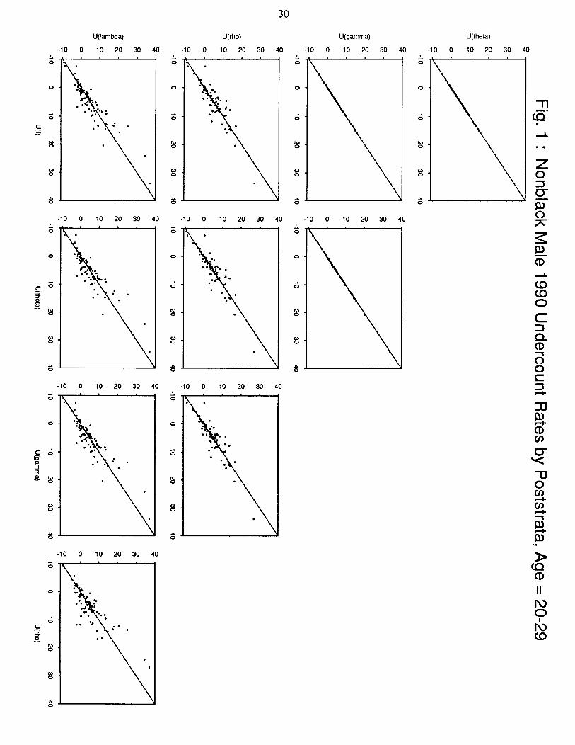
The alternative DSEs were used to produce corresponding estimates of census
undercount rates, lOO(1 - fi/cen), where ten is the census count, and fi any of the DSEs in
Table 1. This was done for males by poststrata, and the resulting undercount rates for the
adult age groups are plotted in the accompanying graphs. The labelling of the graphs is as
follows: U(1) denotes the undercount rates corresponding to $, U(theta) those
corresponding to fi[, etc. Each point in the graphs corresponds to a particular male
poststratum for either nonblacks or blacks. Several “combined” poststrata were split as
discussed in section 5.3. In total, there turn out to be 94 separate nonblack poststrata and
33 separate black poststrata for each age group. Three poststrata with undercounts for all
the estimators lower than -25% (overcounts) have been omitted from the graphs to
improve clarity. Examination of data for these poststrata revealed no explanation for these
“outliers.” Also, three points were omitted from graphs involving Up for which Uf: > 50%.
There was no ready explanation for these “outliers” either, although one can observe from
the graphs that fi[ seems more prone to producing extreme undercount rates than do the
other DSEs.
Figures 1. through 8. show male undercount rates for one estimator plotted against
those of another, for all possible pairs of the five estimators listed in Table 1, for each adult
age group. A 45 degree line (y=x) is provided for reference in all the plots. The set of
plots in the first column of any one of the graphs shows how each of the undercount rates
for the alternative DSEs compares with U1 for a particular age group. For nonblack males
age 20-29, the points in the plots lie mostly near the 45 degree line. For nonblack males 30
and older, or for black males 20 and older, many of the points in the plots lie considerably
above the 45 degree line, reflecting the significant correlation bias in l?: estimated by the
alternative DSEs.

12
The remaining 3x3 triangle of plots for any given age show to what extent the
undercount rates for the different alternative DSEs are similar. In these plots, the points
are scattered about both sides of the 45 degree line, as they effectively must be since all the
alternative estimators must yield the same national total population for males to maintain
the DA sex ratios. The graphs show some variation between the alternative estimators,
but, except for nonblack males age 20-29 for which little correlation bias was estimated,
the variation between undercount rates for alternative estimators is generally less than the
amount by which the undercount rates for the alternative estimators differ from fil.
In PES planning, a decision was made to use the DSE assuming independence, rather
than any of the alternative DSEs, as the production PES estimator. The alternative DSEs
were used for evaluation purposes, however, including the production of estimates for males
of the correlation bias parameter r = ?22/;Ci2 - 1 being used in total error model
evaluations as described in detail by Mulry and Spencer (1990). Here we let ji22 denote an
aggregation over poststrata of the (2,2) cell estimates for any of the alternative DSEs not
to the national level, but to what are called “evaluation poststrata.” Similarly, the Eii22%
are aggregated to x1 ’ 22 s for evaluation poststrata. There are 13 evaluation poststrata and
they are classified as minority (numbers 1,3,5,8,11), these including aggregates of
individual black, Hispanic, and Asian poststrata, or as nonminority (all others). We
produced estimates of r by age groups for each evaluation poststrata from the four
alternative DSEs. These estimates and their standard errors obtained by replication using
VPLX are shown in Table 4. Notice that i corresponding to Ne is constant over all
nonminority evaluation poststrata for a given age. This is because 7 = 0 - 1, so assuming 0
constant within age-race implies 7 constant within age-race. Thus, for all nonminority
evaluation poststrata, ;i = 3 - 1 is constant within age groups. For minority evaluation
poststrata, which are composed partly of blacks and partly of nonblacks, ;i is a weighted
average of the B - 1 values for blacks and nonblacks, with the weights varying across

13
evaluation poststrata depending on their black-nonblack composition.
Table 4 shows considerable variation in ? depending on which alternative DSE is
used, reflecting sensitivity to the assumptions underlying the different estimators. There
are also a number of cases of unusual estimates of 7 (e.g. ? > 10) and of very large
standard errors for ?. This instability is sometimes due to large amounts of sampling error,
and may also be due to other data limitiations, including those discussed in the following
section. The most stable estimates of 7 are the Fe’s, due to the relation between 7 and 0
discussed in the preceeding paragraph. Thus, Fe may provide some useful information
about correlation bias as defined by Mulry and Spencer, but we also see inferences which
might be drawn about r are sensitive to the assumptions made and subject to data
limitations.
5. SOME LIMITATIONS OF THE METHODOLOGY
One obvious general limitation to the methodology presented here is that different
assumptions lead to different estimators and produce different results. Furthermore, there
is no way with our available data to confirm or refute the assumptions underlying any of
the alternative estimators. However, it should also be kept in mind that assuming
independence (no correlation bias) is even more restrictive, and does appear to be refuted
for adult males by the data (subject to limitations of data quality including those discussed
below). Another general limitation of the methodology presented here is that it provides
alternative estimators, and resulting estimates of correlation bias, only for males, and does
so by assuming no correlation bias for females. The reason for this is related to the
limitations of demographic analysis discussed next.
5.1 Some Limitations of Demogranhic Analvsis
Demographic analysis provides population estimates through estimates of the

14
components of population change and the basic accounting identity:
Populatior+ = PopulationtSl + Birthst - Deathst + Immigratior+ - Emmigratior+ .
The generalization of this identity to the age-specific or age-race-sex specific setting is
fairly obvious. By pushing the time of the origin population back, only the components of
change are relevant - e.g. everyone under 65 years of age in 1990 was born after 1925.
The estimates of these components of population change are the basis for using
demographic analysis to evaluate coverage of the 1990 census for the population under 65,
with data from Medicare enrollment used to supplement the information on the 65 and
over population.
Errors in demographic analysis estimates of population arise from errors in the
estimates of the components. Das Gupta (1991) suggests that the most important of these
are errors in corrections for incompleteness of birth registration (particularly for blacks),
errors in estimates of undocumented immigration, and errors in estimates of emmigration.
It is believed that, for the most part, these errors are not differential by sex (see, however,
Robinson, Das Gupta, and Ahmed (1990) for an exception), and so do not much affect sex
ratios (number of males/number of females) derived from demographic analysis. It is
primarily for this reason that we use sex ratios rather than population totals from
demographic analysis. Also, the estimators developed here, if based on demographic
analysis population totals, would be directly sensitive to errors in these totals. This seems
an undesirable property, especially since there is some reliance in demographic analysis on
subjective judgments about levels of emmigration and undocumented immigration.
Difficulties in racial classification restrict demographic analysis to a racial
stratification of just black-nonblack. Even this has become more difficult in recent years
with increasing numbers of births to interracial couples.

15
A full discussion of demographic analysis, its errors, and its usefulness in measuring
census coverage is beyond the scope of this paper. For more details see Fay, Passel, and
Robinson (1988), Clogg, Himes, and Dajani (1990)) Das Gupta (1991)) and Passe1 (1990).
5.2 Dealing with xl2 <A
Another important limitation is the occurrence of poststratum 2x2 tables with
xl2 < 0, particularly for males. (We drop the k subscript here for convenience.) Recall
xl2 = x1+ -xll, where x1+ is the census count less imputations (ten) less an estimate of
erroneous enumerations, and x1 1 is the estimate of census-PES matches. In more detail,
x1+ = cen(1 - EE/Etot) where EE is the E-sample weighted estimate of erroneous
enumerations in the poststratum, and Etot is the corresponding E-sample weighted
population estimate. Theoretically, xl2 > 0, but xl2 < 0 can arise due to sampling error in
xll, EE, and Etot. This occurred in about one-fourth of the male age-race-state tables for
the 1980 PEP 3-8 data. A number of these occurrences involved presumably small sample
sizes (e.g. tables for blacks in states with small black populations), so fewer occurrences of
xl2 < 0 were expected in 1990. However, contrary to expectations, about one-third of the
2x2 tables in 1990 had xl2 < 0. Exact counts by age-race-sex are given in Table 5.
One approach to dealing with this problem is to use a different estimate of x1+, and
consequently of xl2 = x 1+
- xll. A logical choice uses Etot in place of ten in estimating
x1+, i.e. x1+ = Etot(1 - EE/Etot) = Etot - EE. Since xll, EE, and Etot all derive from
the same sample of blocks, one might expect positive correlation in their sampling errors
that would tend to reduce the number of occurrences of xl2 < 0, relative to results
obtained using ten rather than Etot. Unfortunately, this was not the case. Table 5 shows
that roughly the same proportion of poststrata had xl2 < 0 whether census counts or
E-sample totals were used in estimating the in-census margins. Thus, we have not
bothered to compute DSEs using the Etot-based estimate of xl+. It is also worth

16
mentioning that the poststrata with xl2 < 0 for one estimate of x1+ were frequently not
the same ones with xl2 < 0 for the other estimate of x1+.
As described in section 2.1, when xl2 < 0, we reset xl2 = 0 and rescale the first
column (the “in PES” column) of the 2x2 table by xl+/xll. This modification does not
affect the DSEs assuming independence, but it creates an artificial situation for the
alternative DSEs, since they explicitly use the three observed cells of the 2x2 tables, and
not just the marginal totals and matches. The sizable number of tables with xl2 < 0 raises
a difficult question as to whether the alternative DSEs perform sensibly in these cases.
Further research will examine alternate ways to define the sample-weighted estimation of
the 2x2 table entries to avoid or reduce the occurrences of xl2 < 0; until then, this remains
a significant limitation to our analysis.
5.3 Dealing with “Combined” and “Collapsed” Poststrata
The methodology of section 3 assumes that all PES poststrata can be classified as
exclusively black or nonblack. However, of the 116 original poststratum “groups” (sets of
12 poststrata defined identically except for the 12 age-sex categories), 11 of these were
“combined” poststratum groups that included both blacks and nonblacks (9 of which were
combined black-Hispanic poststratum groups). Combined poststrata were defined in areas
of the country where preliminary population estimates suggested the black (or Hispanic)
population was too small to yield adequate PES sample size for separate estimation.
Direct estimates of the xij’s for separate black and nonblack 2x2 tables were unavailable in
combined poststrata. To produce separate 2x2 tables, the combined 2x2 table was split
PrOpOrtiOnd t0 the black and nonblack census COUntS (Say, cenB k and cenNB k)) which . .
B were available. Thus, xkij = xkij (cenB,k/cenk) and x~~j = Xkij cenNB,k/cenk), where ‘(
ten k = cenB’k + ten NB k. (we did not remove imputations from the census counts used,
’ which would have made little difference, nor did we remove estimates of erroneous

17
enumerations, which were not available separately.) This splitting of the combined 2x2
table yields the same results for fil as what was done for the production DSEs, which was
t0 use the same “adjustment faCtOr," AFk = ti:/cenk) for both blacks and nonblacks.
Then I%: k = AFk
fi:(cenN~,k/cenk),
X ceng k = fii(ceng,k/cenk) and fiiD,k = AFk , x CenNB,k =
which is also what would be obtained for $A k -1 ,
and NND,k from our
splitting of the 2x2 table for the combined poststratum.
An analogous situation arose with poststrata that were tlcollapsedl’ across age or sex,
since the methodology of section 3 assumes all poststrata involve a single age-sex group.
Fifteen PES poststrata were collapsed with another poststratum over sex or age, mostly
because of insufficient PES sample size without the collapsing. Most of these involved
collapsing males 65+ in a poststratum group with the corresponding females 65+; a few
cases involved collapsing over age groups. The resulting collapsed 2x2 tables were split
apart proportional to the appropriate census counts, analogous to what was done with the
2x2 tables for “combined” poststrata. Again, this is in the same spirit as what would be
done for collapsed poststrata with the DSE assuming independence.
6. SUMMARY AND CONCLUSIONS
Demographic analysis sex ratios for adult ages at the national level for 1990 differ
significantly from those from the 1990 PES. Comparison of DA and PES national
population totals suggests independence of inclusion in the census and PES may not be a
bad assumption for females. Consequently, while the differences in sex ratios could be due
to a variety of errors in the census, DA, or PES, a leading explanation is correlation bias
for adult males in the PES. Section 3 develops a methodology that attempts to address the
correlation bias problem by defining alternative dual system estimators for males that are
constrained to reproduce the national DA sex ratios for age-race groups. Analogous
methods could be used to constrain to DA population totals; this was not done here

18
because DA totals are believed to be subject to considerably more error than the DA sex
ratios, and use of DA totals would directly transmit such errors to the resulting estimators.
The alternative DSEs proposed assume some function of the 2x2 table probabilities (a
parameter) is constant across male poststrata within age-race groups. Different choices of
such functions lead to different estimators. The parameters are then estimated by
constraining the alternative DSEs to reproduce the DA sex ratios. This generalizes an
approach of Wolter (1990) in (1) generating a whole family of estimators for consideration
that result from different assumptions about what parameter is constant over poststrata,
and (2) providing a method for estimation at subnational levels.
Four alternative DSEs corresponding to four different parametric functions assumed
constant over poststrata were applied to the 1990 PES data. These estimators produced
considerably higher undercount rates for black males 20 and older, and for nonblack males
30 and older, than did the DSE assuming independence. The differences between the
alternative DSEs were generally smaller than the differences between them and the DSE
assuming independence.
There are several important limitations to the results presented here. First, the
methodology is limited by the quality of the DA sex ratios, which we have not discussed in
detail. Second, different assumptions lead to different alternative estimators and different
results, and our available data cannot support any one alternative estimator over any
other. Such considerations must also recognize however, that the assumption of
independence made by the usual DSE is even more restrictive, and appears to be refuted by
the data for adult males. Finally, ad-hoc methods were used to deal with 2x2 tables for
which xl2 < 0. Because this occurred in about one third of the 2x2 tables, this must be
regarded as a significant limitation to our results. Work is currently underway on an
alternative approach to estimating the entries of the 2x2 tables in a way that will generally
avoid the problem of xl2 < 0.

19
Appendix: Bias in l?’ for Fixed 0 Under Possible Heteroneneitv and Dependence
For simplicity of notation we drop the k subscript; it is to be understood here that we
are dealing with a single poststratum. We consider the bias in the context of the DSE
given by (3.1) for a given fixed (not estimated) 0. Our basic result is that,
-8 E(N -
) -N = NpZ2 [B/B-l] + O(1) where 8 = PllP22/P12P21- (A4
In (A.l) the pij = NV% p!‘. are the probabilities in the “average table,” and Lindexes l lJ
individuals in the poststratum with probabilities pt that are allowed to exhibit both
dependence (pt # pf+~:~) and heterogeneity (p~j # Pf; for e # I’) . We see. fie is biased
unless we use B = 8, which is the cross-product ratio in the average table. Also, setting
e = 1 gives
Eue - N = ND22 [P12P21/P11P22 - 11 + O(1) (A-2)
If heterogeneity is present, but independence holds for all individuals 1, then (A.2) reduces
to an expression for the “correlation bias” given by Sekar and Deming (1949) and Wolter
(1986, eq. (2.2)).
Proof of Results:
From (3.1) it is easy to see that
E[fie] = N + E[&i2 - x22] , (A.3)
-e so the bias in N is the same as that in Et ;2 = $2 = @y12/xll)* We expand
g(xll,x12,x21) = x21~12/~ll in a Taylor series about mll,m12,1fi21, where ~ij = NPij =

20
zp!. = 1 1J E$jl = E[xijl)
and where xfj is 1 if the bh individual falls in cell (i,j) of the table
(which occurs with probability pt) and 0 otherwise. This yields the following:
where I%. . is between x.. and m.. for (i,j) = (l,l),( 1,2),(2,1). 13 1J ‘3
For the above we assume ml1
and xl1 (and hence fill) are bounded away from 0. Notice that ml1 = 0 would imply
lj 11 = 0 and then pfl = 0 for all L, so this assumption seems sensible.
Assuming different individuals behave independently, i.e. x~j is independent of x~: j,
as long as L # .P , we have
Var(xij) = !Zpe.(l-pfj) = NPij - Npfj - N{N-‘X(P!.)~ - Fuji L lJ e lJ
= NPij(l-Pij) - N{N-1~(p~j-~ij)2~
I NPij(l-Dij)
< N/4.
It then follows that 1 E[(xij-mij)(xi, j,-mi, j,)] ] < N/4 for all i,j,i’,j’, Using this and
taking the expectation of (A.4)) we get when replacing the iiiij by Npij:
%(xlp12’x21N = w$$&/P11) + O(1)
where O(1) remains bounded as N + 00. Therefore, since 8 is fixed, for large N we get
21
w&l -x221 = N%jZ1P12/P11) - NP22 + O(1).
From (A.3) we see this confirms the expression (A.l) for E[$e].
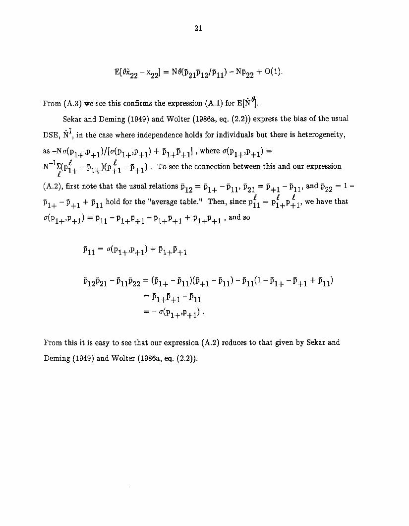
Sekar and Deming (1949) and Wolter (1986a, eq. (2.2)) express the bias of the usual
DSE, fil, in the case where independence holds for individuals but there is heterogeneity,
as -N~(P~+,P+~)/[~(P~+,P+~) + P~+P+~I , where ~(P~+,P+~) =
N-lX( p’ l 1+ - pl+)(p:l - p+l) . To see the connection between this and our expression
(A.2)) first note that the usual relations p,, = pl+ - pll, p21 = p+l - pll, and p22 = l-
p,, - P+1 + Pll hold for the “average table.” Then, since pfl = pf+pfl, we have that
~(P~+,P+~) = Pll - P1+P+l - P1+P+l + Pl+P+, , and so
iill = a(Pl+,P+l) + P1+P+1
p12p21 - PllP22 = 61, - rQ(P+1- Pl,) - Pll(l - Pl, - P+1 + Pll)
= Pl+I’+l - Pll
= - a(P1+,P+l )*
From this it is easy to see that our expression (A.2) reduces to that given by Sekar and
Deming (1949) and Wolter (1986a, eq. (2.2)).

22
REFERENCES
Bell, W. R. and Diffendal, G. J. (1990) “Using Information from Demographic Analysis in Post-Enumeration Survey (PES) Estimation,” paper presented at the annual meeting of the American Statistical Association, August 1990, Anaheim, California.
Choi, C. Y., Steel, D. G., and Skinner, T. J. (1988) “Adjusting the 1986 Australian Census Count for Under-Enumeration,” Survev Methodolopv, 14, 173-190.
Clogg, C. C., C. L. Himes, and A. N. Dajani (1990) “An Evaluation of the Logic, Assumptions, Procedures, and Available Documentation for Demographic Analysis as a Method for Estimating Population by Age, Sex, and Race,” report on phase I of a joint statistical agreement between the U. S. Census Bureau and Pennsylvania State University on Analysis Estimates of Population”,
“Evaluating and Improving Demographic
Pennsylvania State University. Population Issues Research Center,
Cohen, M. L. and Zhang, X. D. (1989) “Three Issues Concerning Coverage Evaluation in the Census,” Proceedings of the Fifth Annual Research Conference, U. S. Department of Commerce, Bureau of the Census, 176-191.
Das Gupta, P. (1991) “Total Error in the Demographic Estimates of Population,” report on demographic analysis evaluation project D-11, U. S. Department of Commerce, Bureau of the Census.
Fay, R. E. (1990) “Draft Documentation of VPLX,” U. S. Department of Commerce, Bureau of the Census.
Fay, R. E., J. S. Passel, and J. G. Robinson (1988) “The Coverage of Population in the 1980 Census,” Evaluation and Research Report PHC80-E4, U. S. Department of Commerce, Bureau of the Census.
Hogan, H. (1990) “The 1990 PES: An Overview,” Proceedings of the American Statistical Association, Survey Research Methods Section.
Isaki, C. T. and Schultz, L. K. (1986) “Dual System Estimation Using Demographic Analysis Data,” Journal of Official Statistics, 2, 169-179.
Muir T
, M. H. and Spencer, B. D. (1990) “Total Error in Post Enumeration Survey PES) Estimates of Population: The Dress Rehearsal Census of 1988,”
Proceedings of the 1990 Annual Research Conference, U. S. Department of Commerce, Bureau of the Census, 326361.
Passel, J. S. (1990) “Demographic Analysis: A Report on Its Utility for Adjusting the 1990 Census,” report to the Special Advisory Panel to the U. S. Department of Commerce, The Urban Institute.

23
Robinson, J. G., P. Das Gupta, and B. Ahmed (1990) “A Case Study in the Investigation of Errors in Estimates of Coverage Based on Demographic Analysis: Black Adults Aged 30 to 64 in 1980,” paper presented at the annual meeting of the American Statistical Association, August 1990, Anaheim, California.
Sekar, C. C. and Deming, W. E. (1949) “On a Method of Estimating Birth and Death Rates and the Extent of Registration,” Journal of the American Statistical Association, 44, 101-115.
Wolter, K. M. (1986) “Some Coverage Error Models for Census Data,” Journal of the American Statistical Association, 81, 338-353.
Wolter, K. M. (1990) “Capture-Recapture Estimation in the Presence of a Known Sex Ratio,” Biometrics, 46, 157-162.

1.
2.
3.
4.
5.
24
Table 1
Alternative Dual System Estimates and their Underlying Assumptions
Estimator
fil = x(1) + g2
AI where x22 = x12x21/xll
Assumntion
Independence
. NB = x(1)
AI + &22 e = p11p22/p12p21 constant over poststrata
CT = fil + (3”1)[x21 + “i2] 7 = p11p2+/p1+p21 constant over poststrata
= P(in PES Iin census)/P(in PES ] not in census)
tip = “(l)/(l - 6m22) p = pm22/pf22 constant over poststrata
,. NX = ox;+w1+ -x21) X = pz1/(p1+p2+) constant over poststrata
= P(in PES ] out of census)/P(in census)
Table 2
Data for 1990 from the census, the Post Enumeration Survey (PES), and Demographic Analysis (DA)
a. Sex Ratios:
Age Census
o-9 1.053 1.051 1.051 1.023 1.036 1.027 10-19 1.046 1.040 1.043 .994 .993 .994 20-29 1.006 1.019 1.019 .831 .808 .896 30-44 .987 .996 1.014 .807 .837 .907 45-64 .936 .944 .957 .790 .805 .893
65+ .699 .700 .707 .628 .634 .661
Nonblacks PES DA Census
Blacks PES DA

25
Table 2 (continued)
b. Population Totals for Males (in millionsl:
Age Census Nonblacks
PES DA Census
o-9 16.0 16.5 16.4 2.82 3.03 3.10 10-19 15.0 15.2 14.9 2.60 2.73 2.67 20-29 17.2 18.1 17.6 2.28 2.37 2.57 3044 25.7 26.4 26.5 3.00 3.20 3.43 45-64 20.0 20.1 20.5 2.01 2.04 2.28 65+ 11.1 11.0 11.3 .92 .91 .96
C. Population Totals for Females (in millions):
Age Census
o-9 15.2 10-19 14.3 20-29 17.1 3044 26.1 45-64 21.4 65+ 15.9
Nonblacks PES
15.7 14.6 17.8 26.5 21.3 15.7
DA
15.6 14.3 17.2 26.1 21.4 16.0
Not es -*
(1)
(2)
(3)
Census
2.76 2.92 3.02 2.62 2.75 2.68 2.74 2.93 2.87 3.69 3.83 3.78 2.54 2.54 2.55 1.47 1.44 1.45
Blacks PES
Blacks PES
DA
DA
Estimates of the military and institutional population are removed from the census and DA since these populations are not part of the PES universe. For this reason, the figures here will not agree with published census and DA figures that include the military and institutional population.
The census data are also adjusted to try to make them comparable to demographic analysis in regard to age reporting and racial (black-nonblack) classification. Demographic analysis determines race according to the racial classification of births, which shows some systematic differences from responses to the census race question.
The data in the above tables were as of late May 1991. Revisions were later made to the demographic analysis data and to some of the comparability adjustments made to the census data. Thus, the data in these tables should not be taken as any sort of official figures. The changes to the sex ratios, however, were very slight, which is all that matters for the results shown here.

26
Table 3
1990 Parameters for Alternative Dual System Estimators (using demographic analysis sex ratios)
Nonblack:
Sex Ratios
a.Jg DA PES
o-9 1.051 1.051 10-19 1.043 1.040 20-29 1.019 1.019 3044 1.014 .996 45-64 .957 .944
65+ .707 .700
Black. -*
o-9 1.027 1.036 .70 .45 10-19 .994 .993 1.06 .71 20-29 .896 .808 3.45 .81 3044 .907 .837 3.17 .61 45-64 .893 .805 6.26 1.72
65+ .661 .634 3.45 1.22
SexRatios
DA PES
s s.e. i s.e. 2 s.e. A s.e.
1.00 .74 1.00 .072 .96 .64 1.02 .072 1.38 .84 1.03 .077 1.24 .69 .99 .072 1.03 .37 1.00 .053 1.48 .48 1.02 .050 3.54 .79 1.23 .053 5.33 1.16 .85 .043 5.01 1.47 1.26 .073 4.30 1.12 .82 .046 3.32 1.39 1.25 .14 2.71 .80 .77 .079
a s.e. 3
.95 1.01 1.53 1.47 1.91 1.50
s.e. 2, s.e. B s.e.
.079 .66 .36 1.09 .094 .12 1.00 .56 1.02 .12 .12 3.62 .63 .76 .056
.083 4.95 .94 .78 .059 .16 7.79 1.63 .58 .41 .21 3.71 1.12 .68 .lO

27
Table 4
1990 Estimates of Correlation Bias Parameters and their Standard Errors Using Alternative DSE's
Evaluation Poststratum 1 age tau(theta) se tau(gamma) se tautrho) o-9 -0.19 0.40 -0.15
10-19 0.10 0.61 0.10 20-29 1.46 0.64 1.26 30-44 2.25 0.53 1.57 45-64 4.96 1.38 2.91 65+ 2.37 0.96 1.28
Evaluation Poststratum 2 o-9 -0.00 0.73 -0.00
10-19 0.37 0.83 0.54 20-29 0.03 0.37 0.13 30-44 2.53 0.78 10.07 45-64 4.01 1.46 6.04 65+ 2.31 1.39 3.88
Evaluation Poststratum 3 o-9 -0.22 0.41 -0.24
10-19 0.18 0.55 0.26 20-29 1.45 0.70 1.92 30-44 2.29 0.52 2.46 45-64 5.03 1.42 4.69 65+ 2.40 0.95 2.39
Evaluation Poststratum 4 o-9 -0.00 0.73 -0 .oo
10-19 0.37 0.83 0.80 20-29 0.03 0.37 0.03 30-44 2.53 0.78 4.53 45-64 4.01 1.46 10.48 65+ 2.31 1.39 8.16
Evaluation Poststratum 5 o-9 -0.28 0.43 -0.17
10-19 0.05 0.70 0.07 20-29 1.68 0.56 1.35 30-44 2.18 0.59 2.50 45-64 5.22 1.69 9.07 65+ 2.44 1.22 2.15
Evaluation Poststratum 6 o-9 -0.00 0.73 -0.00
10-19 0.37 0.83 0.19 20-29 0.03 0.37 0.02 30-44 2.53 0.78 1.69 45-64 4.01 1.46 2.95 65+ 2.31 1.39 1.24
Evaluation Poststratum 7 o-9 -0.00 0.73 -0.00
10-19 0.37 0.83 0.36 20-29 0.03 0.37 0.12 30-44 2.53 0.78 2.91 45-64 4.01 1.46 3.69 65+ 2.31 1.39 2.34
0.27 -0.52 0.49 -0.10 0.61 1.27 0.54 4.31 1.09 7.62 0.60 2.10
1.66 -0.49 0.66 0.83 3.07 1.25 0.46 1.27 0.77 1.73 1.37 2.05 3.69 7.17 10.20
10.88 0.74 4.35 18.33 21.82 6.50 4.55 6.17 9.78 12.31 5.05 9.30 12.22 4.18 6.75
0.53 0.24 0.87 1.01 1.54 0.80 0.93 1.43 1.80 1.98 1.13 1.19 0.97 2.32 1.96 0.98 1.69 1.33 2.99 1.79 1.90 5.55 3.44 4.01 26.71 1.38 1.71 1.47 2.98 2.57
2.06 0.65 2.47 1.31 4.13 2.13 0.18 1.85 1.11 3.91 0.38 -0.08 0.43 -0.35 0.42 3.06 3.87 3.38 4.09 3.61 9.61 0.12 1.21 11.17 11.22
13.14 7.74 12.02 10.51 18.26
0.28 -0.22 0.49 -0.55 0.34 0.46 -0.20 0.49 -0.38 0.50 0.41 2.21 1.06 1.02 0.90 0.97 2.79 1.56 2.61 1.76 5.92 2.75 2.44 10.40 49.45 1.22 1.28 1.31 1.40 1.39
0.45 -0.55 0.53 -0.19 0.72 0.44 -0.54 0.49 -0.29 0.64 0.26 0.80 0.78 -0.42 0.35 0.75 2.43 1.78 1.09 1.08 1.67 4.30 2.82 2.63 2.18 0.82 1.89 2.76 0.46 0.95
0.90 0.67 1.57 0.18 1.29 0.83 0.49 1.06 -0.09 0.89 1.33 1.09 2.06 2.68 4.41 1.85 1.39 1.66 2.81 2.47 1.64 4.73 2.45 2.97 1.72 1.57 3.25 2.02 1.87 1.62
0% 0.56 0.99 2.48 3.78 1.23
taullambda) se -0.11 0.65 0.14 0.90 2.25 1.82 1.65 1.29 2.75 120.75 1.13 1.37

28
Evaluation Poststratum 8 we tau(theta) se tau(gamma)
-0.31 0.11 3.56 2.00 5.24 1.65
o-9 -0.28 0.44 10-19 0.12 0.60 20-29 2.45 0.89 30-44 2.21 0.56 45-64 5.08 1.49 65+ 2.38 0.93
Evaluation Poststratum 9 o-9 -0.00 0.73
10-19 0.37 0.83 20-29 0.03 0.37 30-44 2.53 0.78 45-64 4.01 1.46 65+ 2.31 1.39
Evaluation Poststratum 10 o-9 -0.00 0.73
10-19 0.37 0.83 20-29 0.03 0.37 30-44 2.53 0.78 45-64 4.01 1.46 65+ 2.31 1.39
Evaluation Poststratum 11 o-9 -0.05 0.61
10-19 0.31 0.69 20-29 0.31 0.39 30-44 2.46 0.65 45-64 4.01 1.47 65+ 2.31 1.38
Evaluation Poststratum 12 o-9 -0.00 0.73
10-19 0.37 0.83 20-29 0.03 0.37 30-44 2.53 0.78 45-64 4.01 1.46 65+ 2.31 1.39
Evaluation Poststratum 13 o-9 -0.00 0.73
10-19 0.37 0.83 20-29 0.03 0.37 30-44 2.53 0.78 45-64 4.01 1.46 65+ 2.31 1.39
05:2 tau(rho)
-0.70 0.62 -0.76 2.06 0.83 0.68 0.38 2.99 2.07 0.90 0.65
05;3 0.51 1.67 1.10 2.98 0.91
taullambda) 0.32 0.12 4.92 1.87 5.14 1.52
1?4 1.05 4.18 1.33
72.00 1.63
-0.00 0.34 -0.46 0.44 -0.59 0.41 0.22 0.50 0.50 1.31 -0.61 0.48 0.01 0.20 0.32 0.69 -0.63 0.25 1.62 0.78 3.64 2.52 0.78 0.99 1.09 0.47 2.33 1.89 0.02 0.48 1.04 0.64 0.55 0.79 0.17 0.60
-0.00 2.53 1.13 2.45 1.31 4.36 1.49 3.60 0.89 1.89 1.99 4.36 0.05 0.60 0.16 0.64 -0.04 0.82 6.11 6.67 1.81 1.91 5.46 7.31
15.71 20.68 6.71 6.94 14.35 20.43 3.59 3.12 1.12 4.60 3.70 3.66
-0.04 0.18 -0.34 0.46 0.10 0.23 0.18 0.80 0.19 0.15 -0.06 0.47 0.84 0.19 2.53 1.47 4.08 2.23 2.17 2.00 2.57 2.34 4.38 4.93
-0.62 0.23 -0.59 0.27 -0.60 0.17 -0.03 0.32 7.03 6848.67 4.68 6.66
-0.00 0.31 -0.08 0.80 -0.77 0.32 0.21 0.49 1.41 2.07 -0.12 0.79 0.02 0.23 -0.25 0.44 -0.33 0.39 3.85 4.38 1.87 2.81 5.89 8.70 5.16 5.57 2.93 5.23 5.18 6.99
10.86 14.24 13.08 15.95 19.28 27.64
-0.00 0.67 0.17 0.97 -0.21 0.87 0.40 0.93 0.33 1.03 0.43 1.38 0.04 0.51 -0.69 0.73 0.13 0.88 6.76 6.60 3.99 3.66 7.64 8.60 6.27 4.76 3.64 3.47 7.36 6.61 2.93 2.32 2.97 2.94 3.02 2.87
Notes: tau(theta), tau(gamma), tau(rho), and tau(lambda) are estimates of the correlation bias parameter tau from the alternative dual system estimators (that control to the demographic analysis sex ratios) corresponding to the constant theta, constant gamma, constant rho, and generalized behavioral response estimators (constant lambda) defined elsewhere.
Evaluation poststrata 1, 3, 5, 8, and 11 are aggregates of minority PES poststrata (black, Hispanic, or As:.an); the other evaluation poststrata are aggregates of nonminority PES poststrata.

29
Table 5
Number of 1990 2x2 Tables with xl2 < 0 by Age-Sex-Race
x1+ = cen( 1-EE/Etot) x1+ = Etot - EE
Nonblacks Blacks Nonblacks &s M E &I E
Blacks M E &I F
o-9 29 35 6 8 24 8 9 lo-19 36 34 12 10 39 z: 14 20-29 3; iii i 1; 22 3044
3:
ii i 3 10
45-64 41 37 10 13 28 1: 8 65+ 39 31 8 7 32 22 7 7
# poststrata in 94 each age-sex-race group
94 33 33 94 94 33 33
The Note: Etot is the sample-weighted total from the E-sample for a given poststratum. two parts of the table show results for two alternative definitions of the in-census marginal total, x1+.
30
0
8
%
U(lambda) U(rho)
-10 0 10 20 30 40 -10 0 10 20 30 40
z
-10 0 10 20 30 40 -10 0 10 20 30 40
U(gamma) U(theta)
-10 0 10 20 30 40 -10 0 10 20 30 40

31
U(lambda)
-20 -10 0 10 20 30 40
1. 0
0
-20 -10 0 10 20 30 40
-20 -10 0 10 20 30 40
-20 -10 0 10 20 30 40
U(rho) U(gamma) U(theta)
-20 -10 0 10 20 30 40 -20 -10 0 10 20 30 40 -20 -10 0 10 20 30 40
-20 -10 0 10 20 30 40 k 0
1. 0
0
;;
8
8
8

32
0
8
8
U(lambda) U(rho)
-20 -10 0 10 20 30 40 -20 -10 0 10 20 30 40
0
8
U(theta)
-20 -10 0 10 20 30 40

33
U(lambda)
-20 0 10 20 30 40 50
0 10 20 30 40 50
-20 0 10 20 30 40 50
-20 0 10 20 30 40 50
-20
U(rho)
0 IO 20 30 40 50
-20 0 10 20 30 40 50
-20 0 10 20 30 40 50
-20
U(gamma) U(theta)
0 10 20 30 40 50 -20 0 10 20 30 40 50

U(lambda) U(rho) Warnma) U(theta)
-10 0 10 20 30 40 50 -10 0 10 20 30 40 xl -10 0 10 20 30 40 50 -10 0 10 20 30 40 50
1. 0 . .
. .

35
U(lambda)
0 10 20 30 40 50 -20
U(rho)
0 10 20 30 40 50
U(gamma) U(theta)
-20 0 10 20 30 40 50 -20 0 10 20 30 40 50
l-l 5’ . m . .
I70

36
U(lambda)
-10 0 10 20 30 40 50
U(rho) U(gamma) U(theta)
-10 0 10 20 30 40 50 -10 0 10 20 30 40 50 -10 0 10 20 30 40 50

37
8
U(iambda) U(rho) U(gamma) U(theta)
-30 -10 0 10 20 30 40 -30 -10 0 10 20 30 40 -30 -10 0 10 20 30 40 -30 -10 0 10 20 30 40