using lidar to analyze vegetation structure and...
TRANSCRIPT
Josh Kelly | Western North Carolina Alliance | July 1, 2014
Using LiDAR to Analyze Vegetation Structure and
Ecological Depature in the Upper Warwoman Watershed, Georgia
PAGE 1
Abstract
Ecological restoration has become one of the guiding principles of National Forest management.
However, it can be difficult to identify a reference or desired condition as a restoration goal, and
furthermore, accurately assessing ecosystem condition is dependent of the quality of the data
available. LANDFIRE Biophysical Settings are computer models that combine scientific research,
historical information, and expert opinion to describe the disturbance probabilities of
ecosystems and simulate a natural range of variation as a restoration target. Ecological zone
maps are the most accurate ecosystem maps available for the Southern Blue Ridge Ecoregion
and can be cross-walked to LANDFIRE Biophysical Settings. Light Detection and Ranging (LiDAR)
data are recognized as one of the most comprehensive and accurate data sources, where
available, for measuring vegetation structure. The current condition of the upper Warwoman
Watershed in Rabun County, Georgia was analyzed with the use of ecological zone maps,
LANDFIRE Biophysical Settings, and LiDAR vegetation models. In total, 4,900 hectares of
Chatahoochee National Forest were evaluated using LiDAR measured height and US Forest
Service stand records to estimate forest age. LiDAR measurements of canopy cover and shrub
density were used to evaluate canopy closure. Of seven forest ecosystems evaluated, five were
found to be highly departed from reference conditions. Age and canopy closure were compared
with NRV conditions predicted by the biophysical settings model to determine the level of
departure with each ecozone. In general, ecosystems with a more frequent historical fire return
interval were more departed from reference conditions than mesic ecosystems. All ecosystems
had less young forest than predicted by Biophysical Setting models, demonstrating a very low
rate of disturbance. All oak and pine ecosystems had canopies that were much more closed than
the reference models,with canopy openings and young forest concentrated in prescribed fire
areas. This study indicates that continued fire management and other techniques that create
and maintain early-seral and open-canopy forest along with the continued restoration of old-
growth conditions on public land in the Warwoman Watershed would be ecologically beneficial.
Introduction
Ecological restoration is a scientific discipline that offers strategies for land management that
can improve the health, productivity, and resilience of ecosystems. One difficulty in ecological
restoration can be identifying conditions to restore ecosystems to. This can be especially
challenging in areas in which it is believed that human influence has caused significant and, in
some cases, undesired, change in ecosystem processes as in much of eastern North America.
LANDFIRE Biophysical Setting models are viable options for addressing the challenges associated
with choosing a reference condition. Biophysical Setting models have been developed for each
ecosystem in the U.S. by regional panels of experts that define the probabilities of disturbances
such as fire, wind, ice, insects, disease, and other natural dynamics. The disturbances are used
as “transitions” between S-classes - successional and structural conditions defined in the models
as “states”. After the state and transition framework of the model has been created and
PAGE 2
probabilities entered into ST-Sim software, the models are run through a thousand year
simulation that predicts the percentages of the various S-classes that would be expected for
each ecosystem today. This becomes the reference, or natural range of variation, for each
ecosystem (Landfire 2013). Stakeholders for the Warwoman Watershed met in January 2014 to
review, revise, and localize the applicable biophysical settings for north Georgia, using models
created for western North Carolina in November 2012 as a starting point.
Compared to previous models, the most significant changes were made to the Low Elevation
Pine BpS. The Low Elevation Pine Model had not been evaluated or peer reviewed since its
original drafting, and new dendrochronological evidence (LaForest 2012) indicates uneven age
structure and lower incidence of stand replacement fire than was incorporated in the original
model. In other systems, results were quite similar to previous modeling despite that addition
of landslide events as a disturbance in cove forests. For all models, fire regimes prior to fire
suppression were used, with frequencies of surface fire, mixed-severity fire, and high-severity
fire conservatively estimated. surface fire and mixed severity fire were much more common
than stand replacement fire in all models.
LiDAR technology has emerged as perhaps the most precise and accurate way to measure the
physical structure of large forested areas and has been used to accurately measure tree height,
canopy closure, basal area, and even coarse woody debris (Hopkins et al. 2009; Lefsky et al.
1999; Suarez et al. 2004; Wulder et al. 2012; Zimble et al. 2003). For northeast Georgia, LiDAR
data were collected in March and April of 2010.
Analyzing the physical structure of ecosystems requires a reliable map of where ecosystems
occur. Fortunately, the Southern Blue Ridge Fire Learning Network has invested substantial
resources into mapping the ecological zones of the study area (Simon et al. 2007; Simon 2011).
Ecological zones are analogous to the concept of ecological systems and represent potential
vegetation rather than existing vegetation. The resultant map products are accurate, consistent
over millions of hectares, and facilitate the analysis of vegetation across a gradient of
productivity in which each ecosystem has a discreet potential for tree growth, tree height, and
natural disturbance.
The eCAP methodology developed by The Nature Conservancy uses Biophysical Settings,
ecosystem maps (in this case, ecozone mapping), an assessment of current ecosystem
conditions, and scenario forecasting to guide land management. This study measures the
ecological departure for the ecosystems in question (Low et al. 2010), however it excludes the
scenario forecasting. Ecological departure is calculated by comparing the current percentage of
s-classes to the reference condition as determined by the biophysical settings models in each
ecosystem. By identifying the most departed ecosystems and the S-classes leading to the
departure of each ecosystem, land managers can prioritize activities so as to decrease the
departure of ecosystems from the natural range of variation.
PAGE 3
Methodology
LiDAR Processing
Raw LiDAR data for the Warwoman Watershed were acquired from Earth Explorer
(http://earthexplorer.usgs.gov/). LiDAR point clouds were processed into canopy height, canopy
cover, and shrub density models with the use of Fusion© Software, a free software package
developed by the University of Washington and the USFS Northwest Research Station. The
LiDAR data from the USGS are in UTM projection, so all LiDAR models are in units of meters.
Canopy height models were produced at 6m pixel size with values <0m and >60m (192’) being
excluded from analysis as the tallest known tree in the ecoregion is 192’ tall (http://www.ents-
bbs.org/viewtopic.php?f=74&t=2423 ). Canopy cover and shrub density models were produced
at 15m pixel size. Percent Canopy cover was determined based on the number of first returns
occurring above 1m in height and percent shrub density was calculated from the number of
total returns between 1 and 5 m above the ground. The three LiDAR vegetation models (canopy
height, canopy cover and shrub density) created in Fusion© were imported into ArcMap as ASCII
files and converted to raster format.
GIS Analysis
Ecozones were first lumped into broader types that could be cross-walked to Biophysical
Settings (see Table 1). A total of 7 ecosystems were then evaluated separately.
In two cases LiDAR data were used to refine Ecozone mapping of ecosystem boundaries. In the
local stakeholder meeting, several participants commented that the Dry-Mesic Oak Hickory
ecosystem appeared to be over-mapped. When analyzed with LiDAR it was evident that a
significant portion of the Dry Mesic OakHickory Ecozone had a canopy height above 30 meters.
While 30m is not uncharacteristic for maximum height in Dry-Mesic Oak-Hickory, large areas of
canopy >30 meters tended to occur on concave and north facing slopes. In the opinion of local
experts, this section of Dry Mesic Oak-Hickory was improperly mapped. The high-canopy
portion of the Dry-Mesic Oak Hickory Ecozone was often adjacent to the Cove Forest Ecozone.
The decision was made to intersect the Dry-Mesic Oak Hickory Ecozone with areas of tree height
greater than 30 meters. Five majority filter operations were performed on pixels in that zone of
overlap to eliminate patches of small pixels, which were then left within the Dry Mesic Oak-
Hickory Ecosystem. The results were then erased from the Dry-Mesic Oak Hickory Ecozone and
added to the Mesic Oak Hickory Ecozone. The total area refined was 1439 acres (582 hectares),
about 16% of the original area of the Dry-Mesic Oak Hickory Ecozone, and within the 80%
accuracy threshold sought by the author of the ecozone maps.
In the case of Cove Forest, all of the Cove Forest associated gridcodes (4, 5, 6 & 29) were lumped
into a single class and then separated into Rich Cove Forest and Acidic Cove Forest ecosystems
based on shrub density. Cove Forest in which shrub density was classified as “high” (>50%) were
PAGE 4
placed in Acidic Cove Forest while Cove Forest with “low” shrub density was placed in Rich Cove
Forest.
Next, the LiDAR vegetation models were reclassified into broad categories and then converted
to polygons. Shrub density below 50% was classified as low and the remainder was classified as
high shrub density. Canopy cover was reclassified into open or closed canopy depending on
whether pixels were below or above 60% canopy cover respectively. Additionaly, canopy height
wassplit into two groups, greater than and less than 5m, with forest < 5 m used to denote the
Early S-Class.
Taking inspiration from previous studies, Canopy height models served as a surrogate for age) in
order to identify the Early S-class,which overlaps but is not necessarily synonymous with
concepts of early successional habitat (Weber & Boss 2009. LiDAR height data alone was used
becausethere has been no commercial logging in the Forest Service portion of the watershed for
20 years and the FS Veg database does not track young forest created by prescribed fire.
Additionally, Forest Service data often overlooks natural disturbances like wind throw,
landslides, insect outbreaks, disease, or individual tree mortality if they occur at a scale smaller
than the stand level.
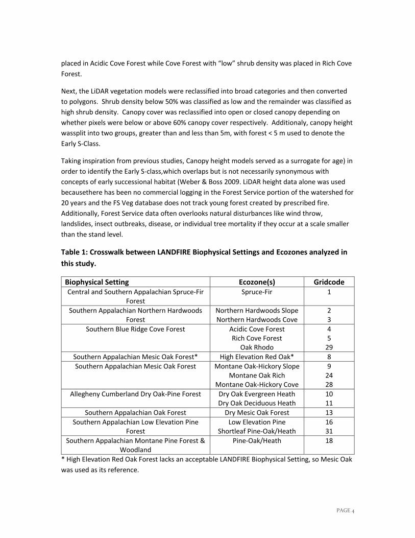
Table 1: Crosswalk between LANDFIRE Biophysical Settings and Ecozones analyzed in
this study.
Biophysical Setting Ecozone(s) Gridcode Central and Southern Appalachian Spruce-Fir
Forest Spruce-Fir 1
Southern Appalachian Northern Hardwoods Forest
Northern Hardwoods Slope Northern Hardwoods Cove
2 3
Southern Blue Ridge Cove Forest Acidic Cove Forest Rich Cove Forest
Oak Rhodo
4 5
29
Southern Appalachian Mesic Oak Forest* High Elevation Red Oak* 8
Southern Appalachian Mesic Oak Forest Montane Oak-Hickory Slope Montane Oak Rich
Montane Oak-Hickory Cove
9 24 28
Allegheny Cumberland Dry Oak-Pine Forest Dry Oak Evergreen Heath Dry Oak Deciduous Heath
10 11
Southern Appalachian Oak Forest Dry Mesic Oak Forest 13
Southern Appalachian Low Elevation Pine Forest
Low Elevation Pine Shortleaf Pine-Oak/Heath
16 31
Southern Appalachian Montane Pine Forest & Woodland
Pine-Oak/Heath 18
* High Elevation Red Oak Forest lacks an acceptable LANDFIRE Biophysical Setting, so Mesic Oak
was used as its reference.
PAGE 5
The remaining forests were reclassified into Mid, Late and Old-growth age classes based on
stand age data extracted from the Forest Service’s FSVeg database, which tracks conditions of
stands throughout Forest Service ownership (see Table 2). These ages are consistent with and
informed by the “Guidance for Conserving and Restoring Old-Growth Forest Communities in the
Southern Region” (USDA Forest Service 1998). Old-growth forest was analyzed in systems in
which LANDFIRE BpS models have been revised during the Cherokee National Forest Landscape
Restoration Initiative and at local workshops in Asheville, NC and Clayton, GA to include old-
growth S-classes.
Once the LiDAR vegetation models were reclassified into broad categories, canopy cover, shrub
density, age data, and ecozone data were intersected to create a single polygon layer. This was
then clipped to a layer of Forest Service ownership. Condition and S-class was determined for
each polygon based on its combination of age, canopy cover and shrub density (see Table 3).
Because Biophysical Setting (BpS) models do not have specific S-classes for shrub density, areas
of high shrub density were aggregated with closed canopied S-classes. High shrub density
generally corresponds to areas of evergreen shrubs in the genera Rhododendron and Kalmia.
These evergreen shrubs tend to exclude many herbs and shade intolerant tree seedlings and
such environments are considered to be ecologically analogous to a closed canopy in this study.
Table 2: Physical Metrics used to define S-classes in this analysis
Ecozone/Ecosystem Max Early-Seral Height
Mid-Seral Age
Old-Growth Age
Canopy Cover Classes
Shrub Density Classes
Acidic Cove* 5 m (16.4’) < 100 years ≥ 140 years <60% = Open
>50% = Acidic Cove
Rich Cove* 5 m (16.4’) < 100 years ≥ 140 years <60% = Open
<50%= Rich Cove
Mesic Oak 5 m (16.4’) < 70 years ≥ 130 years <60% = Open
>50% = High Shrub Cover
Dry Mesic Oak 5 m (16.4’) < 70 years ≥ 130 years <60% = Open
>50% = High Shrub Cover
Dry Oak 5 m (16.4’) < 70 years ≥ 130 years <60% = Open
>50% = High Shrub Cover
Shortleaf Pine 5 m (16.4’) < 70 years ≥ 130 years <60% = Open
>50% = High Shrub Cover
Pine-Oak Heath 5 m (16.4’) < 70 years No BpS Model
<60% = Open
>50% = High Shrub Cover
* Acidic Cove and Rich Cove were separated in this analysis by shrub density; high shrub density
being defined as Acidic Cove
PAGE 6
Finally, the total area of each S-class and each condition class was used to determine the
percentage of each within each ecosystem. The percentages of S-classes measured with LiDAR
were compared with the percentages of S-classes from the Natural Range of Variation described
by BpS models to calculate ecological departure with the following equation:
Ecosystems with a departure scores ≤33% are considered to be consistent with reference
conditions, those with scores 33% ≥ and ≤ 66% are considered to be moderately departed from
reference condition, and scores > 66% reflect high departure from reference conditions.
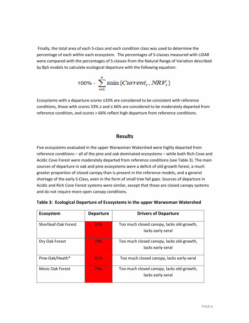
Results
Five ecosystems evaluated in the upper Warwoman Watershed were highly departed from
reference conditions – all of the pine and oak dominated ecosystems – while both Rich Cove and
Acidic Cove Forest were moderately departed from reference conditions (see Table 3). The main
sources of departure in oak and pine ecosystems were a deficit of old-growth forest, a much
greater proportion of closed canopy than is present in the reference models, and a general
shortage of the early S-Class, even in the form of small tree fall gaps. Sources of departure in
Acidic and Rich Cove Forest systems were similar, except that those are closed canopy systems
and do not require more open canopy conditions.
Table 3: Ecological Departure of Ecosystems in the upper Warwoman Watershed
Ecosystem Departure Drivers of Departure
Shortleaf-Oak Forest 83% Too much closed canopy, lacks old-growth,
lacks early-seral
Dry Oak Forest 79% Too much closed canopy, lacks old-growth,
lacks early-seral
Pine-Oak/Heath* 83% Too much closed canopy, lacks early-seral
Mesic Oak Forest 70% Too much closed canopy, lacks old-growth,
lacks early-seral

PAGE 7
Dry-Mesic Oak Hickory
Forest
68% Too much closed canopy, lacks old-growth,
lacks early-seral
Acidic Cove Forest 55% Lacks old-growth, lacks early seral
Rich Cove Forest 53% Lacks old-growth, lacks early seral
* Old-Growth S-classes not included in the Pine/Oak Heath model
The Early S-Class, or areas of forest canopy < 5m tall (16.4’), made up 1.3% of the analysis area
as of 2010 for a total of 172 acres (69.6 ha). This figure is inclusive of maintained wildlife fields
and canopy gaps as small as 36 square meters (387 square feet). Open canopy forest was
likewise a small percentage of the analysis area with 1,072 acres (434 ha) making up 7.9% of
Forest Service ownership in the analysis area. The small percentage of young forest and open-
canopied forest is indicative of a very low level of disturbance in the upper Warwoman
Watershed since the early 1990’s.
Shrub density, or the proportion of LiDAR returns that encountered an object between zero and
five meters, is a measure that is not accounted for in Landfire Biophysical Setting models.
However, it is widely observed that shrub density is high in many parts of the Southern Blue
Ridge and there is evidence that shrub density has increased concurrent with the era of fire
suppression (Pinchot and Ashe 1898; Frost 2000). Somewhat alarmingly, 71% of the upper
Warwoman Watershed had high shrub density (>50% shrub cover) as of April 2010.
While low proportions of young forest and open-canopied forest and a high shrub density
characterize the current condition of the upper Warwoman Watershed, significant differences
were observed between areas inside and outside prescribed fire units. The Early S-Class was
observed to be 12 times more abundant inside prescribed fire units than outside. Open S-
Classes were six times more abundant, the condition of high shrub density was 16% less
abundant, and median shrub density was 10% lower inside prescribed fire units than outside
(See Table 4).
Table 4: Acreages and Relative Percentages of Forest Conditions in the upper
Warwoman Watershed
Rx Fire Units Non-Fire Units Upper Warwoman
Early S-Class Acres 132.9 39.3 172.2
% Early S-Class 4.8% 0.4% 1.3%
Open Canopy Acres 665.3 406.8 1,072.1
% Open Canopy 24% 3.9% 8.1%
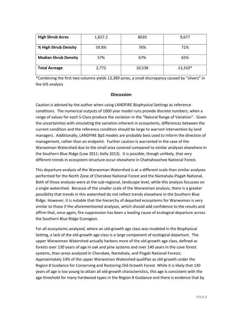
PAGE 8
High Shrub Acres 1,657.2 8020 9,677
% High Shrub Density 59.8% 76% 71%
Median Shrub Density 57% 67% 65%
Total Acreage 2,772 10,538 13,310*
*Combining the first two columns yields 13,389 acres, a small discrepancy caused by “slivers” in
the GIS analysis
Discussion
Caution is advised by the author when using LANDFIRE Biophysical Settings as reference
conditions. The numerical outputs of 1000 year model runs provide discrete numbers, when a
range of values for each S-Class produce the variation in the “Natural Range of Variation”. Given
the uncertainties with simulating the variation inherent in ecosystems, differences between the
current condition and the reference condition should be large to warrant intervention by land
managers. Additionally, LANDFIRE BpS models are probably best used to inform the direction of
management, rather than an endpoint. Further caution is warranted in the case of the
Warwoman Watershed due to the small area covered compared to similar analyses elsewhere in
the Southern Blue Ridge (Low 2011; Kelly 2013). It is possible, though unlikely, that very
different trends in ecosystem structure occur elsewhere in Chattahoochee National Forest.
This departure analysis of the Warwoman Watershed is at a different scale than similar analyses
performed for the North Zone of Cherokee National Forest and the Nantahala-Pisgah National.
Both of those analyses were at the sub-regional, landscape level, while this analysis focusses on
a single watershed. Because of the smaller scale of the Warwoman analysis, there is a greater
possibility that trends in this watershed do not reflect trends elsewhere in the Southern Blue
Ridge. However, it is notable that the hierarchy of departed ecosystems for Warwoman is very
similar to those if the aforementioned analyses, which should add confidence to the results and
affirm that, once again, fire suppression has been a leading cause of ecological departure across
the Southern Blue Ridge Ecoregion.
For all ecosystems analyzed, where an old-growth age class was modeled in the Biophysical
Setting, a lack of the old-growth age class is a large component of ecological departure. The
upper Warwoman Watershed actually harbors more of the old-growth age class, defined as
forests over 130 years of age in oak and pine systems and over 140 years in the cove forest
systems, than areas analyzed in Cherokee, Nantahala, and Pisgah National Forests.
Approximately 14% of the upper Warwoman Watershed qualifies as old-growth under the
Region 8 Guidance for Conserving and Restoring Old-Growth Forest. While it is likely that 130
years of age is too young to attain all old-growth characteristics, this age is consistent with the
age threshold for many hardwood types in the Region 8 Guidance and there is evidence that by
PAGE 9
160 years, some secondary hardwood forests have characteristics of old-growth (USDA 1998;
Scheff 2012). From the standpoint of the eCAP methodology, there is clear justification for
increasing the oldest age classes in all ecosystems at upper Warwoman.
The rate of disturbance is the past several decades has been remarkably low. Even with an
inclusive definition of young forest in which all areas in which the forest canopy is less than five
meters tall were counted, only 1.3% of Forest Service Land in the analysis area is in the Early S-
Class, and most of that occurs in prescribed fire areas. This seems noteworthy, especially given
that the areas as small as 36 m² (387 ft²) were analyzed with LiDAR. Studies on reference sites
in mesic hardwood forests support a constant rate of tree fall disturbance on the order of 2-4%
per decade (Lorimer, Runkle). Given that most of the Southern Blue Ridge was logged in a short
time frame within four decades either side of the turn of the 20th century, it may be that most of
the forest in the upper Warwoman Watershed has not reached an age class in which canopy
trees are falling as frequently as at the study sites. It is also worth noting that only ¼ of the
upper Warwoman Ecosystems fall into the either Mesic Oak-Hickory (1697 acres), Acidic Cove
Forest (1,310 acres), or Rich Cove Forest (198 acres). Very few, if any, studies have examined
the rate of gap formation in submesic to xeric forests in the Southern Appalachians, and it may
be that disturbance in such forests in the absence of fire actually occurs at a lower rate than in
mesic forests. This is a topic worthy of investigation. In any case, there is a striking shortage of
young forest in the upper Warwoman Watershed relative to reference models.
Open S-Classes, or forests with less than 60% canopy closure, are an abundant structural
condition in all of the Biophysical Setting models except for cove forests. According to LiDAR
analysis, 8% of the Forest Service ownership at upper Warwoman qualified as open canopy as of
2010. Values for the total proportion of open-canopy predicted by LANDFIRE BpS models
ranged from 51% open-canopy S-Classes for Mesic Oak Hickory to 92% open-canopy S-Classes
for Shortleaf-Oak. LANDFIRE BpS models predict that 63% of Forest Service ownership in the
upper Warwoman Watershed based on 1000 year model runs. Like, young forest, open-canopy
forest is dependent on disturbance and edaphic factors like thin soil and rock. The lack of open
canopy relative to LANDFIRE BpS models reflects that the rate of disturbance for the past
several decades has been lower than the probabilities of disturbance used in the models. A
reduction in the frequency and extent of fire since the time of Federal ownership in the early
20th century one factor that has allowed forest canopies to close, and an absence of fire and
other disturbance has kept canopies closed.
In addition to historical accounts and modeling efforts, evidence can be found that fire can play
a large role in influencing the structure of Southern Blue Ridge forests in comparing areas that
have experienced fire to those that have not. In the upper Warwoman Watershed, it is clear
that prescribed fire has influenced forest structure, mostly by increasing light penetration,
decreasing shrub cover, and increasing the proportion of regenerating forest (see Table 4).
Prescribed fire has clearly been the most impactful vegetation management activity at upper
Warwoman in recent times and this should be welcome news to fire ecologists and
PAGE 10
Chattahoochee, though it may cause worries among those that are skeptical of the role of fire in
eastern ecosystems (Matlack 2013). The fact that prescribed fire is having an effect on
vegetation structure is indicative of the fact that prescribed fire has been successful in
diversifying structural conditions where it has been applied. As an added benefit, reduction of
shrub cover would likely mean a decrease in fuel loading and severe fire behavior if continued
over the long-term.
Works Cited
Clark, Matthew, David Clark and Dar Roberts. 2004. Small-footprint LiDAR estimation of sub-canopy
elevation and tree height in a tropical rain forest landscape. Remote Sensing of Environment 91
68-89
Harding, D.J., Ma Lefsky, G.G. Parker, and J.B. Blair. 2001. Laser altimeter canopy height methods and
validation for closed-canopy broadleaf forests. Remote Sensing of Environment 76: 283-297
Hopkinson, Chris, and Laura Chasmer. 2009. Testing LiDAR Models of Fractional Cover Across
Multiple Forest Ecozones. Remote Sensing of Environment 113 (1) (January 15): 275–288.
Hunter, William C., David Buehler, Ronald Canterbury, John Confer, and Paul Hamel. 2001.
Conservation of disturbance dependent birds in eastern North America. Wildlife Society Bulletin,
29(2): 440-455
Hyde, P., R. Dubayah, B. Peterson, J.B. Blair, M. Hofton, C. Hunsaker, R. Knox, and W. Walker. 2005.
Mapping Forest Structure for Wildlife Habitat Analysis Using Waveform Lidar: Validation of
Montane Ecosystems. Remote Sensing of Environment 96 (3–4) (June 30): 427–437.
doi:10.1016/j.rse.2005.03.005.
Junttila, Virpi, Andrew O. Finley, John B. Bradford, and Tuomo Kauranne. 2013. “Strategies for
Minimizing Sample Size for Use in Airborne LiDAR-based Forest Inventory.” Forest Ecology and
Management 292 (0) (March 15): 75–85
Kane, Van R., Jonathan D. Bakker, Robert J. McGaughey, James A. Lutz, Rolf F. Gersonde, and Jerry F.
Franklin. 2010. Examining conifer canopy structural complexity across forest ages and elevations
with LiDAR data. Canadian Journal Of Forest Research 40, no. 4: 774-787. Lefsky, Michael A., D.
Harding, W.B. Cohen, G. Parker, and H.H. Shugart. 1999. Surface LiDAR Remote Sensing of Basal
Area and Biomass in Deciduous Forests of Eastern Maryland. Remote Sensing of Environment 67:
83-98
Litvaitis, John A. 2001. Importance of early successional habitats to mammals in eastern forests.
Wildlife Society Bulletin. 29(2): 466-473.
Lefsky, Michael A., Warren B. Cohen, and Geoffrey G. Parker. 2002. Lidar remote sensing for
ecosystem studies. Bioscience52, no. 1: 19-30.
PAGE 11
Loudermilk, E.L., W.P. Cropper Jr., R.J. Mitchell, and H. Lee. 2011. Longleaf Pine (Pinus Palustris) and
Hardwood Dynamics in a Fire-maintained Ecosystem: A Simulation Approach. Ecological
Modelling 222 (15) (August 10): 2733–2750.
Lovell, J.L., D.L.B. Jupp, G.J. Newnham, and D.S. Culvenor. 2011. Measuring Tree Stem Diameters
Using Intensity Profiles from Ground-based Scanning Lidar from a Fixed Viewpoint. ISPRS
Journal of Photogrammetry and Remote Sensing 66 (1) (January): 46–55. Marek K. Jakubowski,
Qinghua Guo, Maggi Kelly, Tradeoffs between lidar pulse density and forest measurement
accuracy, Remote Sensing of Environment, Volume 130, 15 March 2013, Pages 245-253,
Low, Greg, Provencher, and Abele. 2010. Enhanced Conservation Action Planning: Assessing
Landscape Condition and Predicting Benefits of Conservation Strategies. Journal of Conservation
Planning Vol. 6 (2010) 36—60
Martinuzzi, Sebastián, Lee A. Vierling, William A. Gould, Michael J. Falkowski, Jeffrey S. Evans, Andrew
T. Hudak, and Kerri T. Vierling. 2009. Mapping Snags and Understory Shrubs for a LiDAR-based
Assessment of Wildlife Habitat Suitability. Remote Sensing of Environment 113 (12) (December
15): 2533–2546.
Newfont, Katherine. 2012. Blue Ridge Commons: Environmental Activism and Forest History in
Western North Carolina. University of Georgia Press: Athens, Georgia.
Richardson, Jeffrey J, and L. Monika Moskal. 2011. Strengths and Limitations of Assessing Forest
Density and Spatial Configuration with Aerial LiDAR. Remote Sensing of Environment 115 (10)
(October 17): 2640–2651
Simon, Steven A.; Collins, Thomas K.; Kauffman, Gary L.; McNab, W. Henry; Ulrey, Christopher J.
2005., “Ecological Zones in the Southern Appalachians; First Approximation”, Res. Pap. SRS-41.
Asheville, NC: U.S. Department of Agriculture, Forest Service, Southern Research Station. 41 p
Simon, Steven A. 2011. Ecological Zones in the Southern Appalachians; Third Approximation. Report
to Nanthalal-Pisgah National Forest.
Stephens, Peter R., Mark O. Kimberley, Peter N. Beets, Thomas S.H. Paul, Nigel Searles, Alan Bell, Cris
Brack, and James Broadley. 2012. Airborne Scanning LiDAR in a Double Sampling Forest Carbon
Inventory. Remote Sensing of Urban Environments 117 (0) (February 15): 348–357.
Suarez, Juan C., Carlos Ontiveros, Steve Smith, and Stewart Snape. 2004. The Use of Airborne LiDAR
and Aerial Photography in the Estimation of Invidual Tree Heights in Forestry. 7th AGILE
Conference on Geographic Information Science 19 April – 1 May 2004, Heraklion, Greece
Vega, Cedric and Benoit St- Onge. 2009. Mapping site index and age by linking a time series of canopy
height models with growth curves. Forest Ecology and Management. 257: 951-959.

PAGE 12
Weber, Theodore C., and Daniel E. Boss. 2009. Use of LiDAR and Supplemental Data to Estimate
Forest Maturity in Charles County, MD, USA. Forest Ecology and Management 258 (9) (October
10): 2068–2075. doi:10.1016/j.foreco.2009.08.001.
Wulder, Michael A., Joanne C. White, Ross F. Nelson, Erik Næsset, Hans Ole Ørka, Nicholas C. Coops,
Thomas Hilker, Christopher W. Bater, and Terje Gobakken. 2012. Lidar Sampling for Large-area
Forest Characterization: A Review. Remote Sensing of Environment 121 (0) (June): 196–209.
Zimble, Daniel A., David L. Evans, George C. Carlson, Robert C. Parker, Stephen C. Grado, and Patrick
D. Gerard. 2003. Characterizing Vertical Forest Structure Using Small-footprint Airborne LiDAR.
Remote Sensing of Environment 87 (2–3) (October 15): 171–182.
“Using LiDAR to Analyze Forest Structure and Ecological Departure in the Upper Warwoman
Watershed, GA” is supported by Promoting Ecosystem Resiliency through Collaboration:
Landscapes, Learning and Restoration, a cooperative agreement between The Nature
Conservancy, USDA Forest Service and agencies of the Department of the Interior. For more
information, contact Lynn Decker at ldecker @ tnc.org or (801) 320-0524.
In accordance with Federal law and U.S. Department of Agriculture policy, this institution is prohibited from discriminating on the basis of race, color, national origin, sex, age, or disability. (Not all prohibited bases apply to all programs.)
To file a complaint of discrimination, write USDA, Director, Office of Civil Rights, Room 326-W, Whitten Building, 1400 Independence Avenue SW, Washington, DC 20250-9410 or call (202) 720-5964 (voice and TDD). USDA is an equal opportunity provider and employer.