Using Machine Learning to Predict Path-Based Slackfrom Graph-Based Timing Analysis

Andrew B. Kahng†‡, Uday Mallappa‡, Lawrence Saul††CSE and ‡ECE Departments, UC San Diego, La Jolla, CA, USA

{abk, umallapp, saul}@ucsd.edu

Abstract—With diminishing margins in advanced technologynodes, accuracy of timing analysis is a serious concern. Improvedaccuracy helps to reduce overdesign, particularly in P&R-basedoptimization and timing closure steps, but comes at the cost ofruntime. A major factor in accurate estimation of timing slack,especially for low-voltage corners, is the propagation of transitiontime. In graph-based analysis (GBA), worst-case transition timeis propagated through a given gate, independent of the pathunder analysis, and is hence pessimistic. The timing pessimismresults in overdesign and/or inability to fully recover power andarea during optimization. In path-based analysis (PBA), path-specific transition times are propagated, reducing pessimism.However, PBA incurs severe (4X or more) runtime overheadsrelative to GBA, and is often avoided in the early stages ofphysical implementation. With numerous operating corners, useof PBA is even more burdensome. In this paper, we proposea machine learning model, based on bigrams of path stages,to predict expensive PBA results from relatively inexpensiveGBA results. We identify electrical and structural features ofthe circuit that affect PBA-GBA divergence with respect toendpoint arrival times. We use GBA and PBA analysis of agiven testcase design along with artificially generated timingpaths, in combination with a classification and regression tree(CART) approach, to develop a predictive model for PBA-GBAdivergence. Empirical studies demonstrate that our model hasthe potential to substantially reduce pessimism while retainingthe lower turnaround time of GBA analysis. For example, amodel trained on a post-CTS and tested on a post-route databasefor the leon3mp design in 28nm FDSOI foundry enablementreduces divergence from true PBA slack (i.e., model predictiondivergence, versus GBA divergence) from 9.43ps to 6.06ps (meanabsolute error), 26.79ps to 19.72ps (99th percentile error), and50.78ps to 39.46ps (maximum error).

I. INTRODUCTION

Long runtimes of modern electronic design automation(EDA) tools for designs with over a million instances andmany multi-corner multi-mode (MCMM) timing scenariosblock quick turnaround time in system-on-chip (SOC) design.A significant portion of runtime is spent on analysis oftiming across multiple process, voltage and temperature (PVT)corners. At the same time, accurate, signoff-quality timinganalysis is essential during place-and-route and optimizationsteps, to avoid loops in the flow as well as overdesign thatwastes area and power. Tools such as [20] and [21] supportgraph-based analysis (GBA) and path-based analysis (PBA)modes in static timing analysis (STA), enabling a tradeoff ofaccuracy versus turnaround time.

In GBA mode, pessimistic transition time is propagated ateach node of the timing graph. Figure 1(a) illustrates transitionpropagation from launch flip-flop L2 to capture flip-flop C1.At instance A1, the worst of its input transition times ispropagated from input to output. However, the worst transitiontime occurs on the pin that is not part of the L2-C1 timing path.Since cell delay estimation is a function of input transitiontime, the GBA-mode delay calculation for instance A2 isperformed using a pessimistic transition time. This pessimismaccumulates along the timing path, leading to pessimistic

(a)

(b)

Fig. 1. Transition propagation in (a) GBA mode and (b) PBA mode.

arrival time calculation at the endpoint. Further, the transitiontime at the endpoint influences the setup requirement of flip-flop C1, adding further pessimism to the reported slack of thetiming path.

In PBA mode, path-specific transition time is propagated ateach node of the timing graph. Figure 1(b) illustrates transitionpropagation for the L2-C1 timing path in PBA mode. Forinstance A1, actual path-specific transition time is propagated,and is therefore used in the cell delay calculation for A2.As the number of timing paths to an endpoint increases,there is an exponential increase in possibilities of transitionpropagation and delay calculation at each node.1 The path-specific transition propagation and arrival time estimation ateach node is runtime-intensive. Figure 2 shows that for publicbenchmark designs [16] [17] [19] implemented in a 28nmFDSOI foundry enablement, a commercial signoff STA toolexhibits slowdowns (PBA runtime, relative to GBA runtime) ashigh as 15X for leon3mp [19] (108K flip-flops, 450K signalnets), and 150X for megaboom [17] (350K flip-flops, 960Ksignal nets).2 The need for faster path-based analysis is calledout in, e.g., Molina [4]; Kahng [5] names prediction of PBAslacks from GBA analysis as a key near-term challenge formachine learning in IC implementation.

Modern IC implementation in advanced nodes relies onMCMM analysis and PBA mode for signoff. Thus, if PBAwere to be “fast” (i.e., without significant runtime or other

1Details of PBA are given in proprietary tool documentation of major EDAvendors, and analysis outcomes typically have subtle differences across tools.

2This slowdown is seen with “exhaustive” and“slack_greater_than -1” PBA, which assures accuracy in thepath-based analysis and provides the least pessimistic basis for optimization.Because runtimes are so long with exhaustive mode, users must typically use“path” mode in which path-specific timing recalculation is performed onlyfor some set of timing paths. Analysis using path mode does not guaranteeto report worst possible paths to a given endpoint of interest, but can have aslittle as 2X runtime overhead (pba_mode path and nworst 1) versusGBA.

603

2018 IEEE 36th International Conference on Computer Design

2576-6996/18/$31.00 ©2018 IEEEDOI 10.1109/ICCD.2018.00096

Fig. 2. Ratio of PBA runtime to GBA runtime on log scale (commercialsignoff STA tool; 28nm FDSOI foundry enablement) for public-domain designexamples (see Table V for details) ranging in size from 4K flip-flops and 40Kinstances to 350K flip-flops and 990K instances.

overheads) relative to GBA, then only PBA would be used.Unfortunately, today’s PBA runtime overheads force the de-sign methodology to make difficult accuracy-runtime tradeoffchoices. If there is a high timing violation count in earlyphases of physical implementation, timing analysis accuracymay not be a primary concern. Hence, designers will typicallyuse less-accurate but relatively inexpensive GBA mode in theearly stages of design. Later in the design cycle, as the designconverges towards fewer violations, designers must enablePBA mode, at a minimum for timing paths which fail in GBAmode, so as to obtain less-pessimistic, path-specific timingslacks and prevent over-fixing.3 However, by this time, damagehas already been done to the design’s power and area metricsas a result of performing GBA-driven optimizations.

Figure 3 illustrates the magnitude of PBA-GBA divergenceusing a commercial signoff timer for the megaboom test-case implemented in 28nm FDSOI. One worst GBA pathis extracted per endpoint (corresponding to “nworst 1” incommonly-used STA tool Tcl), and the top 15K timing pathsare plotted in decreasing order of PBA-GBA divergence (bythe nature of PBA and GBA, the latter is always pessimisticwith respect to the former). The maximum PBA-GBA diver-gence of 110ps means that the GBA can be pessimistic by110ps as compared to PBA, for this testcase.

Fig. 3. PBA-GBA divergence for the megaboom design (350K flip-flops,990K instances) signed off at 1.2ns clock period in 28nm FDSOI technology.

3The turnaround time overheads of PBA are compounded by having manyMCMM scenarios in timing closure during final stages of implementation,especially for low-power, high-performance designs in advanced nodes.

We emphasize that PBA-GBA divergence is costly – interms of design quality and/or design schedule – in all con-texts. More specifically:

• if GBA slack is positive and PBA slack is positive, thendivergence of slack values reduces the ability to exploitavailable timing slack during power optimization in GBAmode;

• if GBA slack is negative and PBA slack is positive, thenthe divergence in GBA results in fixing of false violations,with attendant schedule, area and power impacts; and

• if GBA slack is negative and PBA slack is negative, thenthe divergence in GBA results in over-fixing of timingviolations, again impacting schedule, power and area.

Thus, predicting PBA without significant runtime overhead canenable improvement of design quality and schedule, indepen-dent of timing slack value. This strongly motivates our presentwork to develop a fast predictor of PBA from GBA analysis.

In the following, we define PBA-GBA path arrival timedivergence as the arrival time change at the endpoint of atiming path in PBA mode as compared to GBA mode. Wecan think of this as a path-consistent juxtaposition of thetwo analyses. Similarly, we define PBA-GBA transition timedivergence for an arc of a timing path as the delta betweentransition time in PBA mode as compared to GBA mode. Anendpoint-consistent definition of divergence is also possible:for endpoint consistency, we define PBA-GBA endpoint arrivaltime divergence as the arrival time difference at a givenendpoint between the worst timing path reported by PBA, andthe worst timing path reported by GBA. Our work assumesthat the clock path does not undergo a significant changein PBA mode as compared to GBA mode. A clock networkis primarily comprised of single-input cells, which results infewer transition propagation conflicts except for rise and fallconflicts. In addition, the sharper (smaller) transition timesrequired in the clock network are more resistant to PBA-GBA variation.4 With this assumption, we approximate PBA-GBA endpoint slack divergence as PBA-GBA endpoint arrivaltime divergence. Unless specified, we use the term “PBA-GBA divergence” to indicate PBA-GBA path arrival timedivergence.The major contributions of our work include the following.

• To our knowledge, we are the first to develop a predictorof PBA from GBA, addressing a challenge noted in [4]and [5] and potentially reducing overdesign as well asdesign schedule.

• We propose a novel combination of bigram-based pathmodeling, classification and regression trees, and selec-tion of model features available from GBA.

• We perform studies in a 28nm FDSOI foundry enable-ment with a range of open benchmark designs, anddemonstrate significant reductions of pessimism, withoutsignificant runtime overhead.

The remainder of our paper is organized as follows. In Sec-tion II, we introduce terminologies, then elaborate on the back-ground of the PBA-GBA divergence problem before formallydefining our problem statement. In Section III, we describeour modeling methodology and model feature selection. In

4Our background studies confirm that the change in clock skew in PBAmode is insignificant.

604

Section IV, we describe our experimental validation setup andresults, along with challenges yet unaddressed by our modelingapproach. Section V concludes with directions for ongoing andfuture research.

II. BACKGROUND

Table I introduces the terminologies and definitions we usein our work.

TABLE ITERMS AND DEFINITIONS.

Term DefinitionBigram or bigram unit Two consecutive (cell) stages in a timing pathAT Arrival timeTR Transition timePD Propagation delaySL Timing slackCL[j] Load capacitance of a driving instance (cell) jFO[j] Fanout of driver cell jDR[j] Drive strength of instance jNm Number of stages in a timing pathNs[j] Stage depth of instance j relative to launch flopNbg Number of bigrams in a timing pathG[j] (Logical) functionality of an instance jATgba[i, j] (ATpba[i, j]) AT of instance j, pin i in GBA (PBA) modeTRgba[i, j] (TRpba[i, j]) TR of instance j, pin i in GBA (PBA) modeTR MAXgba[j] maxi{TRgba[i, j]}ΔTR[i, j] TRgba[i, j] − TRpba[i, j]

TR ratgba[i, j] 1 − TRgba[i,j]

TR MAXgba[i,j](TR ratio)

Acc TR ratgba[i, j]∑Ns[j]

0 TR ratgba[i, j] (accum. TR ratio)PDgba[j] (PDpba[j]) PD of an instance j in GBA (PBA) modeSLgba[j] (SLpba[j]) SL of an endpoint j in GBA (PBA) modeΔPD[j] PDgba[j] − PDpba[j]ΔAT [i, j] ATgba[i, j] − ATpba[i, j]ΔSL[j] SLgba[j] − SLpba[j]

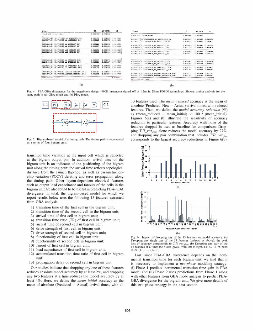
Figures 4(a) and (b) show a timing path trace with endpointarrival times of 1.803ns and 1.693ns in GBA and PBA modes,respectively.5 The PBA-GBA divergence of this timing path is110ps. Pin U1245606/B has a transition time difference of38ps and pin U1245606/Z has an arrival time difference of16ps; these are manifestations of (i) arrival time differencesfrom previous stages and (ii) transition time difference in thecurrent stage due to imbalance in the fanin cone of U1245606.This example highlights the challenge of deciphering graph-based timing analysis reports to estimate hidden path-specifictransition time and arrival time information. Section II-Cbelow discusses electrical and physical features that influencethe PBA-GBA divergence.

Speed, accuracy and scalability of STA has for decades beena focus of industry R&D attention; see, e.g., TAU Workshop[18] presentations. However, there are few prior works onthe use of machine learning for prediction of STA outcomes.Methods to reduce miscorrelation between STA engines orlong optimization runtimes are given by [2] and [3], and[6] seeks to reduce STA runtime itself through distributedcomputing. Kahng et al. [1] provide methodology to modelsignal integrity (SI) effects on path arrival time, using machinelearning. Since their model [1] predicts SI from non-SI, thedegree of pessimism in SI prediction is not a primary concern.However, as noted above, model optimism could be a seriousconcern when predicting PBA from GBA, since an optimisticPBA prediction might mask a real timing violation.

5The path report format shown, as well as certain timing analysis optionnames from tool Tcl mentioned in our discussion, are copyrighted by one ormore EDA companies.

A. Problem Statement

Formally, our problem is: Given a training set Ptrain of(PBA-GBA) path-consistent path analysis pairs, such as thepair shown in Figure 4, use Ptrain to train a learning modelthat predicts PBA-GBA divergence for a testing set Ptest

(where Ptest ∩ Ptrain = ∅) of paths that are analyzed inonly GBA mode. Metrics for evaluation of model quality aredescribed in Section III-A. Experiments used to validate ourmodel are described in Section IV.

B. Intuition for Bigram-Based Modeling

PBA-GBA divergence of a timing path can be estimatedeither stage-wise or path-wise. We refer to the latter approachas lumped path modeling. For stage-wise modeling, n ≥ 1consecutive stages in a timing path are termed an n-gramor n-gram unit within the path. As n increases, stage-wisemodeling (by n-gram units) approaches lumped modeling. Thedefinitions of PBA-GBA divergence in Section I straightfor-wardly extend to stage-wise modeling. The accumulation ofPBA-GBA divergence over the n-grams in a path leads to apath-specific PBA-GBA divergence. Figure 5 shows a bigram-based (n = 2) representation of a timing path from launchflip-flop L1 to capture flip-flop C1.

Based on numerous preliminary studies, we have chosenstage bigrams as the fundamental unit for our modelingapproach. We observe that lumped modeling shields stage-specific details and inter-stage variations, and in our attemptsis prone to large optimistic errors. The lumped approach alsohas a very large space of features (which in general grows withthe number of stages) available to characterize a given path.Furthermore, it is difficult to identify outlier stages that arethe “root causes” of misprediction. By contrast, stage-basedmodeling ensures a fine-grain modeling for each stage andaccounts for inter-stage variation of circuit features. Since pathprediction is an accumulation of stage predictions, boundingstage-wise errors helps limit path mispredictions. (Practically,we find that it is also easier to identify and diagnose outliersin a stage-based model, and to improve the model by addingfeatures that reduce mispredictions for these outliers.)

We also observe that PBA-GBA divergence arises from theexistence of ‘competing’ transition values at inputs of a cell.However, this will be translated into arrival time divergenceonly for the next stage in a given timing path. This naturallymotivates use of a bigram as the basic modeling unit to capturePBA-GBA divergence. We find that the training of n-grammodels for n > 2 is hampered by the combinatorial explosionof possible n-grams (e.g., over a given cell library), whiletraining of bigram models to achieve accurate prediction iscomputationally more tractable.

C. Selection of Features

We have evaluated a comprehensive set of electrical andphysical features of a bigram unit that can affect PBA-GBA divergence. Our analyses indicate that transition timein GBA mode TRgba at the primary input of a bigram unit,and transition time ratio in GBA mode TR ratgba, are twomandatory features that strongly impact PBA-GBA divergenceof the bigram unit. However, these two features alone areinsufficient for accurate prediction of PBA-GBA divergence.Features such as cell drive strength and gate type influence the

605

(a) (b)

Fig. 4. PBA-GBA divergence for the megaboom design (990K instances) signed off at 1.2ns in 28nm FDSOI technology. Shown: timing analysis for thesame path in (a) GBA mode and (b) PBA mode.

Fig. 5. Bigram-based model of a timing path. The timing path is representedas a series of four bigram units.

transition time variation at the input cell which is reflectedat the bigram output pin. In addition, arrival time of thebigram unit is an indicator of the positioning of the bigramunit along the timing path: the arrival time reflects topologicaldistance from the launch flip-flop, as well as parametric on-chip variation (POCV) derating and error propagation alongthe timing path. Other layout-dependent electrical featuressuch as output load capacitance and fanouts of the cells in thebigram unit are also found to be useful in predicting PBA-GBAdivergence. In total, the bigram-based model for which wereport results below uses the following 13 features extractedfrom GBA analysis:

1) transition time of the first cell in the bigram unit;2) transition time of the second cell in the bigram unit;3) arrival time of first cell in bigram unit;4) transition time ratio (TR) of first cell in bigram unit;5) arrival time of second cell in bigram unit;6) drive strength of first cell in bigram unit;7) drive strength of second cell in bigram unit;8) functionality of first cell in bigram unit;9) functionality of second cell in bigram unit;

10) fanout of first cell in bigram unit;11) load capacitance of first cell in bigram unit;12) accumulated transition time ratio of first cell in bigram

unit;13) propagation delay of second cell in bigram unit.

Our studies indicate that dropping any one of these featuresreduces absolute model accuracy by at least 2%, and droppingany two features at a time reduces the model accuracy by atleast 4%. Here, we define the mean initial accuracy as themean of absolute (Predicted − Actual) arrival times, with all

13 features used. The mean reduced accuracy is the mean ofabsolute (Predicted New − Actual) arrival times, with reducedfeatures. Then, we define the model accuracy reduction (%)as (mean reduced − mean initial) × 100 / (mean initial).Figures 6(a) and (b) illustrate the sensitivity of accuracyreduction to particular features. Accuracy with none of thefeatures dropped is used as baseline for comparison. Drop-ping TR ratgba alone reduces the model accuracy by 27%,and dropping any pair combination that includes TR ratgbacorresponds to the largest accuracy reductions in Figure 6(b).

(a)

(b)

Fig. 6. Impact of dropping any of the 13 features on model accuracy. (a)Dropping any single one of the 13 features (indexed as above); the peakloss of accuracy corresponds to TR retgba. (b) Dropping any pair of the13 features at a time; the x-axis gives, from left to right, C(13,2) = 78 pairs(1,2), (1,3), ..., (12,13).

Last, since PBA-GBA divergence depends on the incre-mental transition time for each bigram unit, we find that itis necessary to implement a two-phase modeling strategy:(i) Phase 1 predicts incremental transition time gain in PBAmode, and (ii) Phase 2 uses predictions from Phase 1 alongwith other features from GBA mode analysis to predict PBA-GBA divergence for the bigram unit. We give more details ofthis two-phase strategy in the next section.

606

III. MODELING METHODOLOGY

After selection of features, our modeling methodology in-cludes application of machine learning techniques that capturecomplex interactions of the features and their impact on PBA-GBA divergence. We find that linear regression techniques failto capture nonlinearity of predictions and complex interactionsbetween features. For example, interaction of features suchas input transition, output load and cell drive strength influ-ence PBA-GBA divergence. We have also evaluated nonlinearmodeling techniques such as multivariate adaptive regressionsplines (MARS) [10] which suffer from two-sided distributionof error. Since PBA is always optimistic as compared to GBA,a pessimistic prediction (i.e., prediction of less timing slackthan the given GBA slack) is incorrect. With bigram-basedmodeling, as the number of data points used for modelingincreases (1M+), our results indicate that MARS is not scal-able when higher-order effects are introduced. Ultimately, forimproved accuracy, reduced variance and faster runtimes, wehave focused our efforts on tree ensemble methods. Randomforests of classification and regression trees give the bestresults so far, and Figure 7 illustrates the visual aid inherent intree-based modeling, which helps to better understand featureimportance and classification criteria. We discuss more aboutclassification and regression trees in Section III-B.

Fig. 7. Tree-based classification with 1.7M training samples and 13 features.Feature X[4], which corresponds to TR ratgba, splits the data space into75% and 25% with a split value of 0.493, indicating its importance inclassifying input data.

A. Reporting Metrics

PBA-GBA divergence signifies the pessimism in GBAmode. Therefore, reduction in this pessimism is an appropriatemetric to evaluate the predictive model. Figure 9 shows a path-consistent plot of actual GBA versus PBA path arrival times.The maximum PBA-GBA divergence is 110ps. The blue bandsignifies the pessimism in GBA mode as compared to PBAmode. The intent of machine learning-based PBA predictionis to reduce width of the blue band in a predicted PBA versusactual PBA plot. Ideally, the plot of predicted PBA versusactual PBA would be the straight orange line Y = X , i.e.,zero pessimism in the prediction.

Table II shows actual PBA-GBA divergence metrics froma commercial signoff timer that we use as the reference toquantify the accuracy of our predictive model.

Table III explains path-consistent and endpoint-consistentdivergence metrics that we define for model predictions.

TABLE IIPBA-GBA DIVERGENCE METRICS.

Notation Meaningactual maxpath Upper bound of actual PBA-GBA divergence

actual 99ppath 99th percentile value of sorted PBA-GBA divergence(in ascending order)

actual meanpath Mean absolute value of actual PBA-GBA divergence

These “model *” metrics help assess the divergence of model-predicted PBA timing from actual PBA timing. Metrics thatindicate our model accuracy are 99th percentile value ofdivergence, mean absolute value of divergence, and worst-case prediction divergence. Reduction of “model *” metrics,as compared to reference PBA-GBA divergence “actual *”metrics, shows reduction of pessimism. This is conceptuallyportrayed in Figure 8.

Fig. 8. Reduction of model * metrics as compared to actual * divergencemetrics signifies reduction of pessimism.

TABLE IIIMODEL PREDICTION-BASED DIVERGENCE METRICS.

Notation MeaningPath-consistent prediction metrics

model maxpath Worst-case pessimistic prediction divergencemodel optpath Worst-case optimistic prediction divergence

model 99ppath 99th percentile value of absolute prediction divergencevalues (in ascending order)

model meanpath Mean absolute value of prediction divergence valuesEndpoint-consistent prediction metrics

model maxend Worst-case pessimistic prediction divergencemodel optend Worst-case optimistic prediction divergence

model 99pend 99th percentile value of absolute prediction divergencevalues (in ascending order)

model meanend Mean absolute value of prediction divergence values

Fig. 9. PBA versus GBA path-consistent arrival times (with a maximum PBA-GBA divergence of 110ps) reported by a commercial timer for the megaboomtestcase in 28nm FDSOI technology.

607

B. Classification and regression treesClassification and regression trees (CART) [8] are nonlinear

techniques for constructing predictive models from data. Themodels are obtained by recursively partitioning the data spaceinto feature space and fitting a simple predictive model withineach partition. This recursive partitioning can model a dataset with complex feature interactions. In the context of PBA-GBA prediction, regression trees can be used to predict PBAarrival time for each bigram unit, i.e., we use features of thetest data (GBA analysis results) to predict PBA arrival timefor each data point. Classification trees can predict PBA-GBAdivergence (incremental arrival time gain) where the modeluses features of the test data to predict PBA-GBA divergencefor each data point.

An important realization is that since regression tree-basedmodeling is limited by the span of PBA arrival time values inthe training data, testing is always constrained by the rangeof arrival time values covered in the training phase. On theother hand, classification tree-based modeling is limited by therange of PBA-GBA arrival time increments used in trainingdata. During testing, if a data point exceeds the class valueused in training data, the model is constrained by the span ofincrements in the training data.

As an example, consider a training data set with GBA andPBA arrival time ranges of 24ps to 345ps, and 14ps to 326ps,respectively, along with PBA-GBA divergence range of 0psto 40ps. In regression-based modeling, a test data point withGBA arrival time of 560ps is constrained by the span oftraining data, which is 345ps in this case. In classification-based modeling, predicted PBA-GBA divergence will be fromone of the values in the range of 0ps to 40ps. If we ensurethat the span of possible PBA-GBA divergence values arecovered in the training data, mispredictions can be reduced.In addition, having positive class values gives us “sensibilityby construction” in our predictions, since actual PBA-GBAdivergence can never be negative.

Our preliminary studies, summarized in Table IV for thenetcard testcase, lead us to use the classification tree approachfor PBA-GBA divergence prediction.

TABLE IVREGRESSION VERSUS CLASSIFICATION TREES (NETCARD).

Metric Regression Classificationmodel optpath 18.65ps 8.21psmodel 99ppath 12.96ps 6.44ps

C. Model DefinitionFor Phase 1 and Phase 2 of our modeling, Equations (1)

and (2) capture PBA-GBA divergence in transition time andarrival time respectively, for each bigram unit.

ΔTRbg = f(CL, DR,G, FO, TRgba, ATgba,

TR ratgba, Acc TR ratgba)(1)

ΔATbg = f(CL, DR,G, FO, TRgba, ATgba,

TR ratgba, Acc TR ratgba,ΔTRbg)(2)

PBA-GBA divergence for a timing path is estimated bycumulative addition of bigram PBA-GBA divergence valuesin the timing path. This is explained in Equation (3).

ΔATpath =

Nbg∑

1

ΔATbg (3)

Our model is an ensemble of 50 regression trees.6 We usemean squared error as our criterion for tree splitting, and all13 input features are used in determining a given split point.We do not set any bound on the depth of regression tree, oron the number of leaf nodes for each tree in the ensemble.

D. Modeling Flow

We propose a modeling flow as illustrated in Figure 10.During the model training, both GBA and PBA path-consistenttiming reports are used as inputs. We then extract featuresrequired to model PBA-GBA divergence for each bigrampair. During the model testing, the model predicts PBA-GBA divergence for any unseen (i.e., new) GBA timing path.Predicted PBA timing results that are output by our model cansubsequently serve as, e.g., inputs to optimization and sizingsteps of the physical implementation flow.

Fig. 10. Our modeling flow.

IV. EXPERIMENTAL VALIDATION

We now describe our design of experiments to validate thepredictive model. For each of these experiments, we discussour modeling results.

A. Design of Experiments

Our experiments use in-house developed artificial designsand five real designs as listed in Table V. Artificial designs arecreated for potential availability during an initial, “bootstrap”training phase of modeling. We use 28nm FDSOI foundrytechnology libraries for all our experiments. Training andtest data is split using a random number generator. In ourexperience, the choice of random seed does not significantlyimpact model accuracy. Runtimes on a single thread on anIntel Xeon 2.6 GHz server are as follows. For a trainingdata set with 2.44M bigrams, data preparation time is 362seconds, and model training time is 219 seconds; this is a one-time overhead for realistic use cases. After a trained model isavailable, data preparation time for a test data set with 1.04Mbigrams is 178 seconds, and model inference runtime is 17seconds. For the same testcase, GBA runtime on test datais 156 seconds, whereas PBA runtime is 1080 seconds. Fora design going through optimization phases, recurrent PBA

608

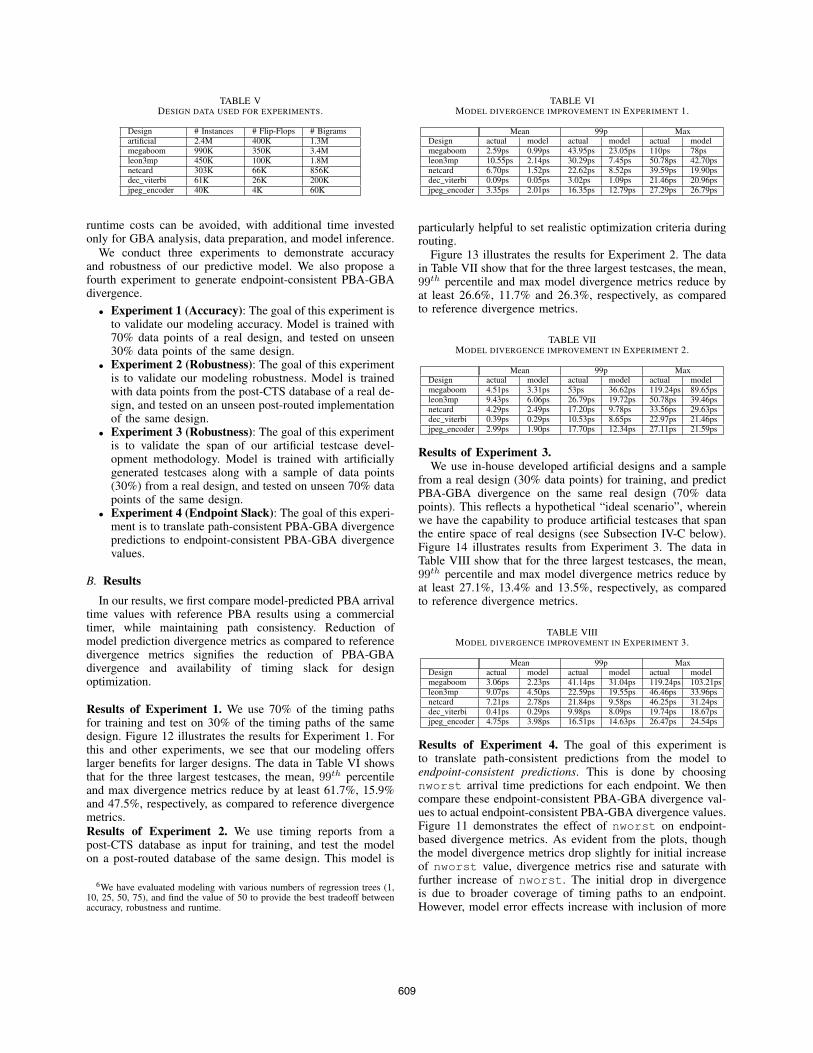
TABLE VDESIGN DATA USED FOR EXPERIMENTS.

Design # Instances # Flip-Flops # Bigramsartificial 2.4M 400K 1.3Mmegaboom 990K 350K 3.4Mleon3mp 450K 100K 1.8Mnetcard 303K 66K 856Kdec viterbi 61K 26K 200Kjpeg encoder 40K 4K 60K

runtime costs can be avoided, with additional time investedonly for GBA analysis, data preparation, and model inference.

We conduct three experiments to demonstrate accuracyand robustness of our predictive model. We also propose afourth experiment to generate endpoint-consistent PBA-GBAdivergence.

• Experiment 1 (Accuracy): The goal of this experiment isto validate our modeling accuracy. Model is trained with70% data points of a real design, and tested on unseen30% data points of the same design.

• Experiment 2 (Robustness): The goal of this experimentis to validate our modeling robustness. Model is trainedwith data points from the post-CTS database of a real de-sign, and tested on an unseen post-routed implementationof the same design.

• Experiment 3 (Robustness): The goal of this experimentis to validate the span of our artificial testcase devel-opment methodology. Model is trained with artificiallygenerated testcases along with a sample of data points(30%) from a real design, and tested on unseen 70% datapoints of the same design.

• Experiment 4 (Endpoint Slack): The goal of this experi-ment is to translate path-consistent PBA-GBA divergencepredictions to endpoint-consistent PBA-GBA divergencevalues.

B. ResultsIn our results, we first compare model-predicted PBA arrival

time values with reference PBA results using a commercialtimer, while maintaining path consistency. Reduction ofmodel prediction divergence metrics as compared to referencedivergence metrics signifies the reduction of PBA-GBAdivergence and availability of timing slack for designoptimization.

Results of Experiment 1. We use 70% of the timing pathsfor training and test on 30% of the timing paths of the samedesign. Figure 12 illustrates the results for Experiment 1. Forthis and other experiments, we see that our modeling offerslarger benefits for larger designs. The data in Table VI showsthat for the three largest testcases, the mean, 99th percentileand max divergence metrics reduce by at least 61.7%, 15.9%and 47.5%, respectively, as compared to reference divergencemetrics.Results of Experiment 2. We use timing reports from apost-CTS database as input for training, and test the modelon a post-routed database of the same design. This model is

6We have evaluated modeling with various numbers of regression trees (1,10, 25, 50, 75), and find the value of 50 to provide the best tradeoff betweenaccuracy, robustness and runtime.

TABLE VIMODEL DIVERGENCE IMPROVEMENT IN EXPERIMENT 1.

Mean 99p MaxDesign actual model actual model actual modelmegaboom 2.59ps 0.99ps 43.95ps 23.05ps 110ps 78psleon3mp 10.55ps 2.14ps 30.29ps 7.45ps 50.78ps 42.70psnetcard 6.70ps 1.52ps 22.62ps 8.52ps 39.59ps 19.90psdec viterbi 0.09ps 0.05ps 3.02ps 1.09ps 21.46ps 20.96psjpeg encoder 3.35ps 2.01ps 16.35ps 12.79ps 27.29ps 26.79ps

particularly helpful to set realistic optimization criteria duringrouting.

Figure 13 illustrates the results for Experiment 2. The datain Table VII show that for the three largest testcases, the mean,99th percentile and max model divergence metrics reduce byat least 26.6%, 11.7% and 26.3%, respectively, as comparedto reference divergence metrics.

TABLE VIIMODEL DIVERGENCE IMPROVEMENT IN EXPERIMENT 2.

Mean 99p MaxDesign actual model actual model actual modelmegaboom 4.51ps 3.31ps 53ps 36.62ps 119.24ps 89.65psleon3mp 9.43ps 6.06ps 26.79ps 19.72ps 50.78ps 39.46psnetcard 4.29ps 2.49ps 17.20ps 9.78ps 33.56ps 29.63psdec viterbi 0.39ps 0.29ps 10.53ps 8.65ps 22.97ps 21.46psjpeg encoder 2.99ps 1.90ps 17.70ps 12.34ps 27.11ps 21.59ps

Results of Experiment 3.We use in-house developed artificial designs and a sample

from a real design (30% data points) for training, and predictPBA-GBA divergence on the same real design (70% datapoints). This reflects a hypothetical “ideal scenario”, whereinwe have the capability to produce artificial testcases that spanthe entire space of real designs (see Subsection IV-C below).Figure 14 illustrates results from Experiment 3. The data inTable VIII show that for the three largest testcases, the mean,99th percentile and max model divergence metrics reduce byat least 27.1%, 13.4% and 13.5%, respectively, as comparedto reference divergence metrics.

TABLE VIIIMODEL DIVERGENCE IMPROVEMENT IN EXPERIMENT 3.

Mean 99p MaxDesign actual model actual model actual modelmegaboom 3.06ps 2.23ps 41.14ps 31.04ps 119.24ps 103.21psleon3mp 9.07ps 4.50ps 22.59ps 19.55ps 46.46ps 33.96psnetcard 7.21ps 2.78ps 21.84ps 9.58ps 46.25ps 31.24psdec viterbi 0.41ps 0.29ps 9.98ps 8.09ps 19.74ps 18.67psjpeg encoder 4.75ps 3.98ps 16.51ps 14.63ps 26.47ps 24.54ps

Results of Experiment 4. The goal of this experiment isto translate path-consistent predictions from the model toendpoint-consistent predictions. This is done by choosingnworst arrival time predictions for each endpoint. We thencompare these endpoint-consistent PBA-GBA divergence val-ues to actual endpoint-consistent PBA-GBA divergence values.Figure 11 demonstrates the effect of nworst on endpoint-based divergence metrics. As evident from the plots, thoughthe model divergence metrics drop slightly for initial increaseof nworst value, divergence metrics rise and saturate withfurther increase of nworst. The initial drop in divergenceis due to broader coverage of timing paths to an endpoint.However, model error effects increase with inclusion of more

609

Fig. 11. Plots of prediction error with nworst of endpoints.

data points (i.e., worst GBA paths) per endpoint, and theendpoint-consistent accuracy metric saturates with increase innworst. Potentially, nworst 3 could be a point of interestto derive endpoint-based arrival time or slack predictions. Atthe same time, achieving better use of, say, nworst 20 GBAanalysis is an important direction for future work.

C. Challenges

Two important remaining challenges for our modelingapproach are (i) the reduction or elimination of remainingoptimism in PBA slack prediction, and (ii) endpoint-consistentpessimism reduction. In this subsection, we provide severalcomments regarding the former challenge.

First, while optimistic predictions are evident in our ex-perimental results, we note that for any endpoint, the arrivaltime gain lower-bounds the slack gain. In other words, forany endpoint, slack gain is likely to be larger than arrival timegain. This is because sharper transition times at the endpointin PBA mode lead to reduction of the setup time requirementat the endpoint. Since our present model predicts arrival timegain, there is actually some leftover “budget” with respect toslack gain prediction – and this in effect reduces the optimismof our model. For the leon3mp testcase, this “budget” averages4.46ps over all endpoints, as plotted in Figure 15.

Second, we observe that misprediction is at least partlya consequence of a test data point’s distance from nearesttraining data points in the modeling feature space. In an idealscenario, our artificial circuits for any (technology and library)design enablement would effectively span (cover) the entirereal design space, such that a one-time trained model couldaccurately predict PBA timing from GBA timing on any realdesign. However, our current artificial circuits methodology isfar from enabling such an ideal use case. Thus, an importantdirection for future work is to incrementally train models withreal design data along with artificial and previous circuit data,always testing on subsequent design iterations. In an extensionof our current approach, test data points encountered that arefar from training data set could be incrementally includedinto the training data set to help reduce model mispredictions.Further, detailed PBA analysis can be performed every fewdesign iterations, to identify mispredicted outliers for inclusionin future (incremental) training. Such a methodology might

follow the flow shown in Figure 16.7 Last, we recall theprimary motivation of reducing overdesign during the opti-mization flow – not replacing the golden signoff tool andPBA signoff analysis. The model calibration flow illustratedin Figure 16 helps make isolated optimistic predictions lesssignificant as compared to the benefits obtained from reducingoverdesign earlier in the design process.

V. CONCLUSIONS

In this work, we are the first to apply machine learningtechniques to model PBA-GBA divergence in endpoint arrivaltimes, addressing an important accuracy-runtime tradeoff instatic timing analysis [4] [5]. We propose a model based ondecision trees along with electrical and physical features ofstage bigrams in timing paths. We assess potential benefits ofour model using 28nm FDSOI foundry technology, a leadingcommercial signoff STA tool, and implementations of publictestcase designs up to 1M+ instances. We measure the decreaseof PBA-GBA divergence obtained by the model, accordingto several metrics and in several usage scenarios. In ourexperiments, model-predicted PBA arrival times reduce mean,99th percentile and max divergence metrics by at least 26.6%,13.4% and 11.7%, respectively as compared to reference PBA-GBA divergence metrics. Such reductions can help avoid over-fixing and achieve improved power and area outcomes duringoptimization. In addition, both model training and inferenceare efficient, with a training time of 219 seconds and inferencetime of 17 seconds for a test data set with 1.04M bigrams.

A number of ongoing and future works remain. (1) We areseeking to integrate our predictive models with an academicsizer and optimizer, to explore the benefit from reducedpessimism in MCMM timing closure and sizing for leakageand total power reduction. (2) As shown by Experiment 3 andas discussed in Subsection IV-C, significant work remains tobe done toward design of artificial testcases that can train well-performing models for a given design enablement, withoutreliance on any actual designs. (3) Reduction or eliminationof remaining optimism in PBA slack prediction, as well asendpoint-consistent pessimism reduction, present additionalchallenges for future research. Both the available “budget”of arrival time gain versus slack gain, and the proposed in-cremental model calibration flow, may provide mitigations forthe problem of optimism. (4) Last, as noted in the Experiment4 discussion, achieving better use of multiple (nworst � 1)GBA paths to a given endpoint is an important direction topursue.

ACKNOWLEDGMENTS

We thank Dr. Tuck-Boon Chan of Qualcomm and Dr. Sid-dhartha Nath for providing valuable feedback. Research in UCSan Diego ABKGroup is supported in part by funding fromNSF, DARPA, Qualcomm, Samsung, NXP, Mentor Graphicsand the C-DEN center.

7A comment: As a design undergoes changes during the design cycle,performing PBA analysis after any given design change would bring sig-nificant runtime overhead. The ultimate bar for value obtained from GBA-based predictive model is faster design convergence through avoidance ofPBA analysis overheads.

610

Fig. 12. Results of Experiment 1 for actual GBA path arrival time (top row) and predicted PBA path arrival time (bottom row) versus actual PBA path arrivaltime for, in left-to-right order, megaboom, leon3mp, netcard, dec viterbi and jpeg encoder.

Fig. 13. Results of Experiment 2 for actual GBA path arrival time (top row) and predicted PBA path arrival time (bottom row) versus actual PBA path arrivaltime for, in left-to-right order, megaboom, leon3mp, netcard, dec viterbi and jpeg encoder.

REFERENCES

[1] A. B. Kahng, M. Luo and S. Nath, “SI for Free: Machine Learning of InterconnectCoupling Delay and Transition Effects”, Proc. SLIP, 2015, pp. 1-8.

[2] A. B. Kahng, S. Kang, H. Lee, S. Nath and J. Wadhwani, “Learning-BasedApproximation of Interconnect Delay and Slew in Signoff Timing Tools”, Proc.SLIP, 2013, pp. 1-8.

[3] S. S. Han, A. B. Kahng, S. Nath and A. Vydyanathan, “A Deep LearningMethodology to Proliferate Golden Signoff Timing”, Proc. DATE, 2014, pp. 1-6.

[4] R. Molina, EDA Vendors Should Improve the Runtime Performance of Path-Based Timing Analysis, http://www.electronicdesign.com/eda/eda-vendors-should-improve-runtime-performance-path-based-analysis, May 2013.

[5] A. B. Kahng, “Machine Learning Applications in Physical Design: Recent Resultsand Directions”, Proc. ISPD, 2018, pp. 68-73.

[6] T.-W. Huang and M. D. F. Wong, “Timing Closure: Speeding Up IncrementalPath-Based Timing Analysis with MapReduce”, Proc. SLIP, 2015, pp. 1-6.

[7] J. Bhasker and R. Chadha, Static Timing Analysis for Nanometer Designs: APractical Approach, Springer, 2009.

[8] L. Breiman, J. H. Friedman, R. A. Olshen and C. J. Stone, Classification andRegression Trees, Chapman & Hall/CRC, 1984.

[9] T. Hastie, R. Tibshirani and J. Friedman, The Elements of Statistical Learning:Data Mining, Inference, and Prediction, Springer, 2009.

[10] J. H. Friedman, “Multivariate Adaptive Regression Splines”, Annals of Statistics19(1) (1991), pp. 1-67.

[11] L. Breiman, “Random Forests”, Machine Learning 45 (2001), pp. 5-32.[12] Synopsys, Inc., https://www.synopsys.com

[13] Cadence Design Systems, Inc., https://www.cadence.com[14] scikit-learn, http://scikit-learn.org[15] PyTorch, https://pytorch.org[16] OpenCores, https://opencores.org[17] RISC-V, https://riscv.org[18] TAU Workshop, https://www.tauworkshop.com[19] M. M. Ozdal, C. Amin, A. Ayupov, S. Burns, G. Wilke and C. Zhuo, “The ISPD-

2012 Discrete Cell Sizing Contest and Benchmark Suite”, Proc. ISPD, 2012, pp.161-164.

[20] Synopsys PrimeTime User Guide, http://www.synopsys.com/Tools/Implementation/SignOff/Pages/PrimeTime.aspx

[21] Cadence Tempus User Guide. https://www.cadence.com/content/cadence-www/global/en US/home/tools/digital-design-and-signoff/silicon-signoff/tempus-timing-signoff-solution.html

611

Fig. 14. Results of Experiment 3 for actual GBA path arrival time (top row) and predicted PBA path arrival time (bottom row) versus actual PBA path arrivaltime for, in left-to-right order, megaboom, leon3mp, netcard, dec viterbi and jpeg encoder.

Fig. 15. Arrival time gain versus slack gain for the leon3mp testcase with anaverage “budget” of 4.46ps (indicated by red arrow) and a maximum “budget”of 17.88ps over 100K endpoints.

Fig. 16. A potential incremental modeling flow to reduce mispredictions.

612