Using Markov Decision Processes to Solve a Portfolio Allocation

Problem

Daniel Bookstaber

April 26, 2005

Contents

1 Introduction 3

2 Defining the Model 42.1 The Stochastic Model for a Single Asset . . . . . . . . . . . . . . . . . . . . . . . . . 4

2.1.1 States: . . . . . . . . . . . . . . . . . . . . . . . . . . . . . . . . . . . . . . . . 42.2 Transitions: . . . . . . . . . . . . . . . . . . . . . . . . . . . . . . . . . . . . . . . . . 42.3 The Markov Decision Process . . . . . . . . . . . . . . . . . . . . . . . . . . . . . . . 5

2.3.1 Decision Epochs: . . . . . . . . . . . . . . . . . . . . . . . . . . . . . . . . . . 52.3.2 States: . . . . . . . . . . . . . . . . . . . . . . . . . . . . . . . . . . . . . . . . 52.3.3 Actions: . . . . . . . . . . . . . . . . . . . . . . . . . . . . . . . . . . . . . . . 52.3.4 Transitions: . . . . . . . . . . . . . . . . . . . . . . . . . . . . . . . . . . . . . 62.3.5 Rewards: . . . . . . . . . . . . . . . . . . . . . . . . . . . . . . . . . . . . . . 62.3.6 Policy: . . . . . . . . . . . . . . . . . . . . . . . . . . . . . . . . . . . . . . . . 62.3.7 Solving for the Optimal Policy Using Value Iteration . . . . . . . . . . . . . . 6

3 Solving the Optimal Policy with a Small State Space 73.1 Assuming a Distribution and Generating Data . . . . . . . . . . . . . . . . . . . . . 73.2 Solving the Optimal Policy with a Model Using Real Data . . . . . . . . . . . . . . . 123.3 The Greedy Policy . . . . . . . . . . . . . . . . . . . . . . . . . . . . . . . . . . . . . 123.4 The Intermediate Heuristic . . . . . . . . . . . . . . . . . . . . . . . . . . . . . . . . 123.5 Value Iteration Policy . . . . . . . . . . . . . . . . . . . . . . . . . . . . . . . . . . . 123.6 Results . . . . . . . . . . . . . . . . . . . . . . . . . . . . . . . . . . . . . . . . . . . . 13

4 Extending the Model to Two Assets 154.1 Defining The Two Stock System . . . . . . . . . . . . . . . . . . . . . . . . . . . . . 154.2 Calculating the MDP Transition Probability Matrix . . . . . . . . . . . . . . . . . . 17

4.2.1 Independent Stocks . . . . . . . . . . . . . . . . . . . . . . . . . . . . . . . . 174.2.2 Moderately Correlated assets . . . . . . . . . . . . . . . . . . . . . . . . . . . 184.2.3 Strongly Correlated assets . . . . . . . . . . . . . . . . . . . . . . . . . . . . . 19

1

4.3 Performance . . . . . . . . . . . . . . . . . . . . . . . . . . . . . . . . . . . . . . . . . 19

5 Defining the Model for the Large State/Action Space 205.1 Action Space . . . . . . . . . . . . . . . . . . . . . . . . . . . . . . . . . . . . . . . . 225.2 State Space . . . . . . . . . . . . . . . . . . . . . . . . . . . . . . . . . . . . . . . . . 24

6 Defining the Constrained Markov Decision Process 256.1 Decision Epochs: . . . . . . . . . . . . . . . . . . . . . . . . . . . . . . . . . . . . . . 256.2 States: . . . . . . . . . . . . . . . . . . . . . . . . . . . . . . . . . . . . . . . . . . . . 256.3 Actions: . . . . . . . . . . . . . . . . . . . . . . . . . . . . . . . . . . . . . . . . . . . 256.4 Transitions: . . . . . . . . . . . . . . . . . . . . . . . . . . . . . . . . . . . . . . . . . 256.5 Rewards: . . . . . . . . . . . . . . . . . . . . . . . . . . . . . . . . . . . . . . . . . . 25

7 Solving an Optimal Policy for the Constrained MDP 267.1 Off-Policy Q-Learning . . . . . . . . . . . . . . . . . . . . . . . . . . . . . . . . . . . 267.2 Sarsa(λ) . . . . . . . . . . . . . . . . . . . . . . . . . . . . . . . . . . . . . . . . . . . 277.3 Approximating the Values for each State . . . . . . . . . . . . . . . . . . . . . . . . . 287.4 Results . . . . . . . . . . . . . . . . . . . . . . . . . . . . . . . . . . . . . . . . . . . . 29

8 Conclusion 30

9 References 32

2

1 Introduction

This paper investigates solutions to a portfolio allocation problem using a Markov Decision Process(MDP) framework. The two challenges for the problem we examine are uncertainty about the valueof assets which follow a stochastic model and a large state/action space that makes it difficult toapply conventional techniques to solve.

The portfolio allocation problem attempts to maximize the return of a portfolio of assets overa finite time horizon, each with an expected return. Specifically, we wish to learn a policy thatoptimally chooses which assets to buy and sell. The appeal of this instance is both the stochasticnature of the problem and the accessibility of real world data to experiment with. We assume wehave a fixed amount of capital and a fixed universe of assets we can buy and sell. We also assumewe are given an expected return for each asset which changes each time period following a welldefined Markov process. The changing expected return of each asset makes the problem stochasticand the large number of assets and possible portfolios creates a large state/action space.

The first part of the paper examines a miniature version of the problem to illustrate conventionalsolutions on both data derived from an assumed distribution and real market data. This is meantto introduce notation, formally specify the MDP and give intuition about the model.

The second part shows why the conventional solutions are intractable for the large state spaceproblem. We then suggest a different framework to model the same problem and present twoalgorithms to solve the model.

3

2 Defining the Model

The portfolio selection model actually consists of two models, one models the stochastic movementof the expected return for each stock and another models the entire portfolio. In this section weformally define both models and the notation that will be used throughout the paper.

2.1 The Stochastic Model for a Single Asset

We define each asset as following a Markov model that transitions each period. Each state of theMarkov model has an expected return associated with it, as well as a standard deviation of theexpected return.

2.1.1 States:

The set of M states the Markov model can take are defined as:

E = {e1, e1, . . . , eM}

Each state, ei, gives an expected return, α̂i, for an asset in state ei. Each state also has a standarddeviation of the expected return, σ̂i, which measures the deviation of actual returns from theexpected return.

2.2 Transitions:

Each time period the asset transitions to either the same state or a new state. If the asset is in stateet at time t, the probability that it transitions to state et+1 at time t+1 is expressed as p(et, et+1).We use a transition probability matrix to describe the set of transition probabilities where the rowdescribes the current state and the column describes the future state:

State e1 e2 · · · eM

e1 p(e1, e1) p(e1, e2) · · · p(e1, eM )e2 p(e2, e1) p(e2, e2) · · · p(e2, eM )...

......

. . ....

eM p(eM , e1) p(eM , e2) · · · p(eM , eM )

Table 1: The transition probability matrix for the Markov model. This gives the probability of anasset transitioning from one state to another for each time period.

The Markov model is an input to the Markov decision process we define below.

4

2.3 The Markov Decision Process

The Markov decision process (MDP) takes the Markov state for each asset with its associatedexpected return and standard deviation and assigns a weight, describing how much of our capitalto invest in that asset. Each state in the MDP contains the current weight invested and theeconomic state of all assets. We also define actions which allow us to modify the weights of assetsfrom period to period. Finally we define rewards which specify how much expected return theportfolio generates in its current state.

2.3.1 Decision Epochs:

The set of decision epochs is defined as:

t = 1, 2, . . . , T

at each decision epoch t we observe the state st, choose an action at and receive a reward rt(s, a)which is a function of the state and action of that decision epoch.

2.3.2 States:

The state space S of the MDP consists of all possible combinations of economic states and weightsfor all stocks in the universe. For simplicity, we allow a discrete set of weights W . If there are Nstocks at time t, the state st of the MDP is the economic state of each stock i at time t, ei,t, andthe proportion of money wi,t, invested in the stock. Explicitly we write st as:

st =((e1,t, . . . , eN,t), (wi,t, . . . , wN,t)

)If there are N stocks where each stock can take M economic states and have W different weights

assigned to it, then the cardinality of the state space for one stock is MW and the cardinality ofthe state space for the MDP is NMW .

2.3.3 Actions:

The action space A consists of all possible actions we can take, where an action means modifying theweights for each stock in the universe. Each decision epoch we take an action, at, which modifiesthe weight assigned to each stock. If there are N stocks, the action at is an N element vectordefined as:

at =(a1,t, . . . aN,t

)where ai,t is the change to the weight of stock i at time t.With N stocks and W different weights, the action space at any given state is NW .

5

2.3.4 Transitions:

Each decision epoch, the MDP transitions to the same state or a new state, depending on thetransitions of the Markov model for each asset in the portfolio and the action we take. If the MDPis at state st at time t, the probability that it transitions to state st+1 at time t + 1 is expressed asp(st, at, st+1).

2.3.5 Rewards:

The reward is the expected return from period t to t + 1 of our portfolio less transaction costs,where the expected return for an individual asset is given by its state. Formally we define thereturn of stock i from t to t + 1 as α̂i.

C(at) is the transaction cost function based on the action we take:

C(at) = c

N∑i=1

|ai,t| (1)

where 0 ≤ c ≤ 1.The reward from stock i currently in state (ei,t, wi,t) when we take action ai,t is defined as:

rt(ei,t, wi,t, at) = (wi,t + ai,t)α̂i,t − C(ai,t) (2)

When dealing with the reward for the entire portfolio, any leftover capital not invested in stocksis invested in a risk free asset giving a risk free rate of return rc. Therefore we can write the rewardfor several stocks as:

rt((~et, ~wt),~at) =[ N∑

i=1

rt(ei,t, wi,t, ai,t

]+ rc ∗ (1−

∑i=1

(wi,t + ai,t)) (3)

2.3.6 Policy:

A policy is a function that maps an action to every state. We say a policy is optimal if it generatesat least as much total reward as all other possible policies.

2.3.7 Solving for the Optimal Policy Using Value Iteration

Using the MDP above, the value iteration algorithm is one conventional method to solve for theoptimal policy. We use the value iteration algorithm suggested by Puterman to find a stationaryε-optimal policy. The algorithm is shown in figure 1.

6

1. Select υ0, specify ε > 0, and set n = 0.

2. For each s ∈ S, compute υn+1(s) by

υn+1(s) = maxa∈As

{r(s, a) +

∑j∈S

λp(j|s, a)υn(j)}

(4)

3. If|υn+1 − υn| < ε(1− λ)/2λ (5)

go to step 4. Otherwise increment n by 1 and return to step 2.

4. For each s ∈ S, choose

dε(s) ∈ arg maxa∈As

{r(s, a) +

∑j∈S

λp(j|s, a)υn+1(j)}

(6)

and stop

Figure 1: The value iteration algorithm, which solves for an optimal policy using a dynamic pro-gramming approach and bootstrapping. This is a good method to use on small state spaces.

3 Solving the Optimal Policy with a Small State Space

In this section we present several methods to find policies for the MDP with a small state space bylimiting the number of assets and allowing only a few discrete weights. We only allow one stock inthe universe and a risk free asset.

3.1 Assuming a Distribution and Generating Data

First we present a simple example with a Markov model we sample from to generate the movementof an asset. We use this example to illustrate the value iteration method. We define a Markovmodel for the asset with 3 states. The expected return associated with each state is given in table2.

State Exp Return0 -.011 .00012 .005

Table 2: The expected return of each state of the Markov model.

We also define a transition probability matrix for the Markov model in table 3. It is importantto note this is only the transition probability matrix for the Markov model states, which comprises

7

only part of the Markov decision process states.

State 0 1 20 .5 .4 .11 .1 .6 .32 .05 .05 .9

Table 3: The transition probability matrix for the Markov model.

Each state of the MDP contains the Markov model state and the weight assigned to the stock.For simplicity, we only allow 3 weights: −1, 0, 1. These weights mean we can use all our money toshort the stock, invest nothing in the stock and everything in cash, or use all our capital to longthe stock.

Therefore we have a total of 9 different MDP states describing the Markov state and weight ofthat asset. We write the entire MDP state space below where for the first number is the Markovstate and the second number if the weight of the asset in our portfolio.

S = {(0,−1), (1,−1), (2,−1), (0, 0), (1, 0), (2, 0), (0, 1), (1, 1), (2, 1)}

We can now explicitly write the transition probability matrix for the Markov decision process.Unfortunately this is very large since each transition depends on the action we take. Therefore weprovide a transition probability matrix for the Markov decision process given a specific action.

Since we limit the investment in the stock to the domain [−1, 1], there is a limited set of actionsfor each state. For example, if our current weight on the stock is -1 with the signal in state i, theavailable set of actions are Ai,−1 = {0, 1, 2}. However if our current weight on the stock is 0, theavailable set of actions are Ai,0 = {−1, 0, 1}. Therefore the tables only show transitions to allowablestates which explains why they are different sizes.

State (0,-1) (1,-1) (2,-1)(0,1) 0.5 0.4 0.1(1,1) 0.1 0.6 0.3(2,1) 0.05 0.05 0.9

Table 4: The transition probability matrix of the MDP when the action is -2

We are now able to apply the value iteration algorithm to our example. We run the algorithmwith the discount factor λ = .95. We specify the cost function as:

C(at) = .003 ∗ at (7)

which means for every 1% of capital we wish to invest, we have to pay .3% in transaction costs.Table 9 shows the convergence of the expected reward for each state every 10 iterations:Table 10 shows the optimal policy mapping an action to each state using step 4 of the algorithm:Not surprisingly, the optimal policy for this simple example is predictable. When the asset is

in the state 0 which predicts a strong negative return, we always perform the action that gives us

8

State (0,-1) (1,-1) (2,-1) (0,0) (1,0) (2,0)(0,0) 0.5 0.4 0.1 0 0 0(1,0) 0.1 0.6 0.3 0 0 0(2,0) 0.05 0.05 0.9 0 0 0(0,1) 0 0 0 0.5 0.4 0.1(1,1) 0 0 0 0.1 0.6 0.3(2,1) 0 0 0 0.05 0.05 0.9

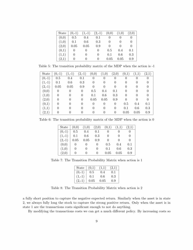
Table 5: The transition probability matrix of the MDP when the action is -1

State (0,-1) (1,-1) (2,-1) (0,0) (1,0) (2,0) (0,1) (1,1) (2,1)(0,-1) 0.5 0.4 0.1 0 0 0 0 0 0(1,-1) 0.1 0.6 0.3 0 0 0 0 0 0(2,-1) 0.05 0.05 0.9 0 0 0 0 0 0(0,0) 0 0 0 0.5 0.4 0.1 0 0 0(1,0) 0 0 0 0.1 0.6 0.3 0 0 0(2,0) 0 0 0 0.05 0.05 0.9 0 0 0(0,1) 0 0 0 0 0 0 0.5 0.4 0.1(1,1) 0 0 0 0 0 0 0.1 0.6 0.3(2,1) 0 0 0 0 0 0 0.05 0.05 0.9

Table 6: The transition probability matrix of the MDP when the action is 0

State (0,0) (1,0) (2,0) (0,1) (1,1) (2,1)(0,-1) 0.5 0.4 0.1 0 0 0(1,-1) 0.1 0.6 0.3 0 0 0(2,-1) 0.05 0.05 0.9 0 0 0(0,0) 0 0 0 0.5 0.4 0.1(1,0) 0 0 0 0.1 0.6 0.3(2,0) 0 0 0 0.05 0.05 0.9

Table 7: The Transition Probability Matrix when action is 1

State (0,1) (1,1) (2,1)(0,-1) 0.5 0.4 0.1(1,-1) 0.1 0.6 0.3(2,-1) 0.05 0.05 0.9

Table 8: The Transition Probability Matrix when action is 2

a fully short position to capture the negative expected return. Similarly when the asset is in state2, we always fully long the stock to capture the strong positive return. Only when the asset is instate 1 are the transactions costs significant enough to not do anything.

By modifying the transactions costs we can get a much different policy. By increasing costs so

9

N State Epsilon(0 -1) (0 0) (0 1) (1 -1) (1 0) (1 1) (2 -1) (2 0) (2 1)

0 0 0 0 0 0 0 0 0 01 0.010 0.007 0.004 0 0 0 -0.001 0.002 0.005 0.01010 0.035 0.032 0.029 0.022 0.024 0.025 0.029 0.032 0.035 0.00320 0.055 0.052 0.049 0.041 0.043 0.044 0.049 0.052 0.055 0.00230 0.066 0.063 0.060 0.052 0.055 0.056 0.060 0.063 0.066 0.0009140 0.073 0.070 0.067 0.059 0.061 0.063 0.067 0.070 0.073 0.0005450 0.077 0.074 0.071 0.064 0.066 0.067 0.072 0.075 0.078 0.0003255 0.079 0.076 0.073 0.065 0.067 0.068 0.073 0.076 0.079 0.00025

Table 9: Iterations of the value iteration algorithm with Cost = .003. We can see the value of eachstate converge towards a stable value.

State Action(0 -1) 0(0 0) -1(0 1) -2(1 -1) 0(1 0) 0(1 1) 0(2 -1) 2(2 0) 1(2 1) 0

Table 10: The optimal policy derived from the value iteration algorithm with cost = .003. Toderive the optimal policy, for each state we choose the action that maximizes the expected rewardas given from the value iteration algorithm.

that C(a) = .04 ∗ a, the new optimal policy changes as shown in table 11.

Table 11: Optimal Policy of Value Iteration with Cost = .04State Action(0 -1) 0(0 0) 0(0 1) 0(1 -1) 0(1 0) 0(1 1) 0(2 -1) 2(2 0) 1(2 1) 0

10

Here we see the only time we act is when the stock is in economic state 2. Perhaps by inspectingthe expected return of every state you would expect the optimal policy to always short the stockwhen in state 0 because of its large return and not act in the other states. However, while the returnisn’t as large as state 0, the probability of staying in state 2 is high enough that we should long thestock because we expect high return for several periods, thus justifying the high transaction costs.

11

3.2 Solving the Optimal Policy with a Model Using Real Data

In this section we use a Markov model derived from real movements of an actual asset. We presenttwo myopic policy-finding heuristics and compare them to the value iteration optimal policy byexamining the cumulative expected return. We can also look at cumulative real return, althoughthis data is much more noisy since it depends on the quality of the assets Markov model. Alsoreal returns are very volatile and a few outlier days can affect the entire history. Finally we canexamine cumulative transaction costs to see how much costs each policy incurs. We ran the analysison Coca-Cola over the time period from 5/21/1998 to 1/27/2005.

3.3 The Greedy Policy

The greedy policy maximizes the one period reward. For each state, we choose the action thatmaximizes reward. Therefore, if there is no expected return greater than transaction costs (whichis often the case) the policy never buys or sells the stock since any action would result in a negativereturn over that period due to transaction costs.

3.4 The Intermediate Heuristic

The intermediate heuristic chooses the action as a mathematical function of the expected return ofthe stock α̂i,t and the transaction cost constant c. The action is defined as:

a = kα̂t

c(8)

where k is a parameter. When k = 1, this policy will always invest in the direction of theexpected return such that the one period return is zero (since it buys as much as the transactionscosts allow). When 0 < k < 1, the policy is more greedy and myopic by always realizing positivereward for the current period but still investing some in the direction of the expected return.Similarly, when k > 1 it becomes less greedy and myopic by accepting a negative reward for thecurrent period and investing more quickly in the stock. In the case when actions are not realnumbers but a discrete set, the action is set to the nearest allowable action.

We solve for the k that maximizes expected return over a sample period using Monte Carlosimulation of the assets Markov model. To choose the optimal value for k, we iterate throughseveral possible values of k. For each k, we use Monte Carlo simulation to create a million days ofasset states using the transition probability matrix for the Markov model. Next we calculate theaverage return over that period using the policy for that k. We then choose the k that maximizedaverage return. The algorithm is given in figure 3.4.

3.5 Value Iteration Policy

To get the optimal value iteration policy, we used λ = .999 for the discount factor with ε = .01 forconvergence. It ran for 3000 iterations before it converged.

12

maxK = 0maxR = 0For each value of k

r = 0s_0 = random economic statew_0 = 0For t = 1 to 1,000,000

s_t = simulated state given s_{t-1}expReturn = expected return of state s_taction a_t = k * expReturn / cround a_t to the nearest allowed actionr = r + r(s_t, a_t)

if(r > maxR)maxR = rmaxK = k

Figure 2: Intermediate Heuristic Algorithm For Optimal k

3.6 Results

Figure 3.6 shows the results of cumulative expected reward for the three different policies. This isthe true test to see which policy is optimal since it was optimized on rewards given from the model.

We see the value iteration optimal policy barely beats the function approximation policy. Thegreedy policy never puts on a trade because the expected return is never greater than the transactioncosts. There are two explanations why the function approximation policy is almost the same as thevalue iteration policy. First, this Markov decision process is very simple, so a heuristic should beable to get close to the optimal policy. Secondly, the function approximation policy was optimizedusing information contained in the transition probability matrix, therefore it is not completelynaive to the behavior of the model. If we just blindly chose a value for k, it would have performedsignificantly worse. The greedy policy is just a straight line because it never invested in the stockand put 100% in the risk free cash investment.

Figure 4 shows the daily weights for each policy, which gives an idea of how quickly the policyreacts to changes in the expected return of the stock. The value iteration is the quickest to changeits weight when the expected return changes. The intermediate heuristic is just a bit slower toadjust the weight which causes it to perform slightly worse. The greedy weight is always zero sincethe expected return never goes above the transaction costs.

Figure 5 shows the cumulative realized reward following the three different policies. Althoughthe cumulative expected reward following the value iteration and intermediate heuristic policiesdon’t differ by much, we see the effects on the realized reward are significant. To calculate realizedreward, we simply substitute the expected return predicted by our model with the actual return ofthe stock over the same period. The greedy policy realized reward is just a straight line because it

13

Figure 3: Cumulative Expected Reward for Coca Cola using 3 different optimal policies

never invests in the stock and therefore receives return .Figure 6 gives the cumulative transactions costs for the three different policies. The greedy

policy never transacts and therefore has no transaction costs. The intermediate heuristic andvalue iteration policies have almost identical costs, although the intermediate heuristic transacts insmaller quantities over a few days rather than once like the value iteration policy does.

14

Figure 4: Daily weight of investment in Coca Cola using 3 different optimal policies

4 Extending the Model to Two Assets

The previous analysis can be extended to the two asset case where each asset follows a differentMarkov process. With more than one asset in the system, we also must consider the relationshipbetween the assets, defined by the conditional transition probabilities. This section shows howto apply the techniques of the previous section to a two asset model and shows the results whenthe policies solved assuming independent assets are applied to dependent assets. We assume atheoretical distribution for each asset.

4.1 Defining The Two Stock System

We use the Markov process presented in the previous section for stock A. The expected returns foreach state of stock A are shown in table 12.

15

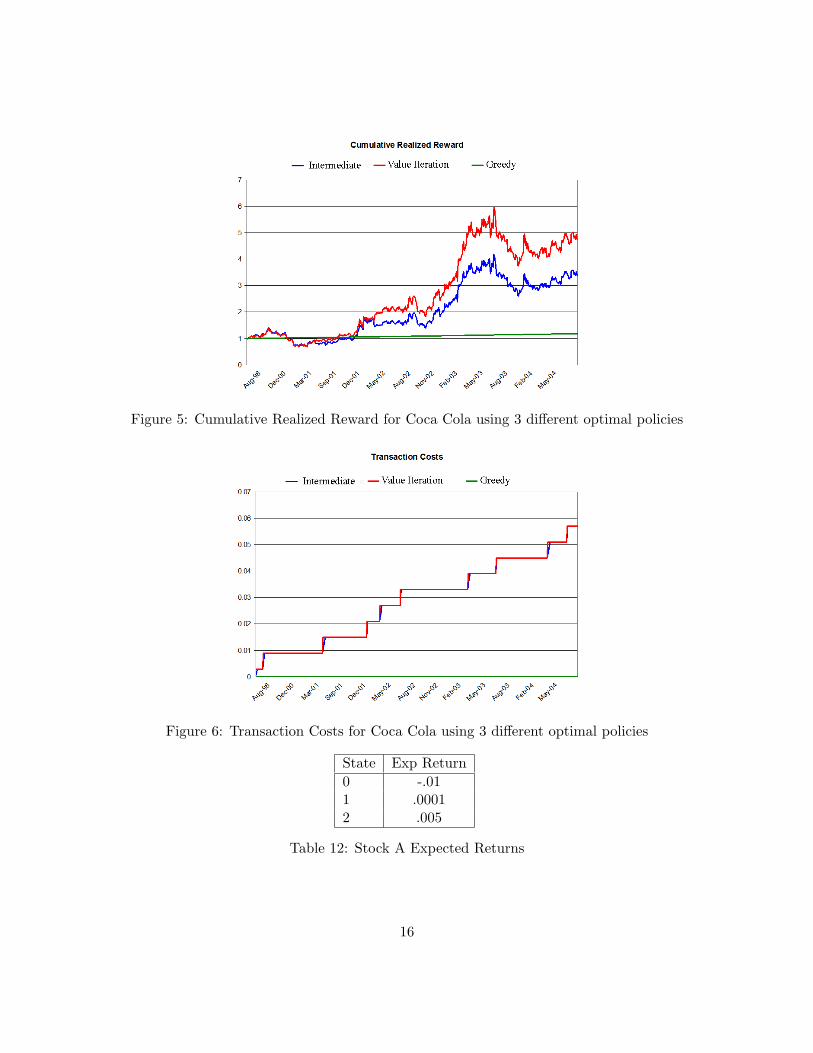
Figure 5: Cumulative Realized Reward for Coca Cola using 3 different optimal policies

Figure 6: Transaction Costs for Coca Cola using 3 different optimal policies

State Exp Return0 -.011 .00012 .005

Table 12: Stock A Expected Returns

16

The transition probability matrix for stock A is given in table 13.

State 0 1 20 .5 .4 .11 .1 .6 .32 .05 .05 .9

Table 13: Stock A Transition Probability Matrix

Next we define the expected returns and transition probability matrix for the second stock. Theexpected returns are shown in table 14. The TPM is given in table 15.

State Exp Return0 -.0021 -.00052 .006

Table 14: Stock B Expected Returns

State 0 1 20 0.2 0.6 0.21 0.5 0.2 0.32 0.1 0.1 0.7

Table 15: Stock B Model Transition Probability Matrix

Assuming we can still hold weights of {−1, 0, 1} as in the previous example for both stocks,the state space for the Markov Decision Process when N = 2, M = 3 and W = 3 is NMW = 512.However we still include the constraint that

∑Ni=1 |wi| ≤ 1 stating we can only invest at most 100%

of our capital. This constraint also reduces the state space. Although the state space has expandedfrom the 1 stock problem, it is still tractable using the methods from the previous section.

4.2 Calculating the MDP Transition Probability Matrix

4.2.1 Independent Stocks

The assumption that the stocks move independently eases the calculation of the transition proba-bility matrix for the MDP. To calculate the transition probability matrix with multiple assets, weneed to include the asset into the subscript of the economic state. Therefore eA,i means asset A isin economic state i. Also we recall that p(eA,i, eA,j) refers to the probability that asset A transitionfrom economic state i to state j. We also note that p({eA,ieB,k}, {eA,jeB,l}) refers to the probabilitythat asset A transitions from economic state i to j and asset B transitions from economic state kto l. Since these events are independent, we can write:

p({eA,ieB,k}, {eA,jeB,l}) = p(eA,i, eA,j) ∗ p(eB,k, eB,l) (9)

17

Using this approach and incorporating the weights as the other part of the MDP state, we cancompute the transition probability matrix for the MDP. Since the state space is much larger, weonly show the transitions of economic states for all combinations of A and B together. This isthe essential data to build the much larger transition probability matrix for the MDP which alsoincorporates weights into the state because these probabilities are then just placed in the propercells since the weights don’t affect transition probabilities. Table 16 shows the joint transitionprobabilities assuming independence based only on the economic state transitions.

A 0 0 0 1 1 1 2 2 2B 0 1 2 0 1 2 0 1 2

0 0 0.1 0.3 0.1 0.08 0.24 0.08 0.02 0.06 0.020 1 0.25 0.1 0.15 0.2 0.08 0.12 0.05 0.02 0.030 2 0.05 0.05 0.4 0.04 0.04 0.32 0.01 0.01 0.081 0 0.02 0.06 0.02 0.12 0.36 0.12 0.06 0.18 0.061 1 0.05 0.02 0.03 0.3 0.12 0.18 0.15 0.06 0.091 2 0.01 0.01 0.08 0.06 0.06 0.48 0.03 0.03 0.242 0 0.01 0.03 0.01 0.01 0.03 0.01 0.18 0.54 0.182 1 0.025 0.01 0.015 0.025 0.01 0.015 0.45 0.18 0.272 2 0.005 0.005 0.04 0.005 0.005 0.04 0.09 0.09 0.72

Table 16: Transition Probability Matrix for a Two Independent asset MDP

4.2.2 Moderately Correlated assets

If the assets are no longer independent but correlated, then we can no longer express the joint tran-sition probabilities as a product of the two individual transition probabilities. For the moderatelycorrelated asset case, we assume asset B transitions independently of asset A but that asset A isconditional on B. Using the law of conditional probability:

p(A ∩B) = P (A)P (B|A)

we can write:

p({eA,ieB,k}, {eA,jeB,l}) = p({eA,i, eA,j}|{eB,k, eB,l})p({eB,k, eB,l}) (10)

To simplify even more, we only condition on the previous state of asset B, not the transition ofasset B. Therefore the final joint probability is written:

p({eA,ieB,k}, {eA,jeB,l}) = p(eA,i, eA,j |eB,k) ∗ p(eB,k, eB,l) (11)

Table 17 shows the joint probabilities p(eA,i, eA,j |eB,k) for the moderate correlation case. Thiscan be compared with table 13 to see the effect effect on asset A.

18

TPM for A given B is in state 0 TPM for A given B is in state 1 TPM for A given B is in state 2State 0 1 2 State 0 1 2 State 0 1 2

0 0.6 0.3 0.1 0 0.2 0.6 0.2 0 0.2 0.4 0.41 0.4 0.4 0.2 1 0.05 0.9 0.05 1 0.1 0.2 0.72 0.3 0.2 0.5 2 0.1 0.8 0.1 2 0.025 0.075 0.9

Table 17: Moderately Correlated Transition Probability Matrix for asset A Conditional on theState of asset B

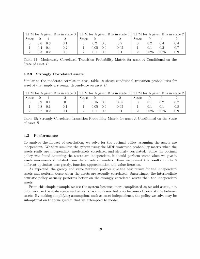
4.2.3 Strongly Correlated assets

Similar to the moderate correlation case, table 18 shows conditional transition probabilities forasset A that imply a stronger dependence on asset B.

TPM for A given B is in state 0 TPM for A given B is in state 1 TPM for A given B is in state 2State 0 1 2 State 0 1 2 State 0 1 2

0 0.9 0.1 0 0 0.15 0.8 0.05 0 0.1 0.2 0.71 0.8 0.1 0.1 1 0.05 0.9 0.05 1 0.1 0.1 0.82 0.7 0.2 0.1 2 0.1 0.8 0.1 2 0.025 0.075 0.9

Table 18: Strongly Correlated Transition Probability Matrix for asset A Conditional on the Stateof asset B

4.3 Performance

To analyze the impact of correlation, we solve for the optimal policy assuming the assets areindependent. We then simulate the system using the MDP transition probability matrix when theassets really are independent, moderately correlated and strongly correlated. Since the optimalpolicy was found assuming the assets are independent, it should perform worse when we give itassets movements simulated from the correlated models. Here we present the results for the 3different optimizations; greedy, function approximation and value iteration.

As expected, the greedy and value iteration policies give the best return for the independentassets and perform worse when the assets are actually correlated. Surprisingly, the intermediateheuristic policy actually performs better on the strongly correlated assets than the independentassets.

From this simple example we see the system becomes more complicated as we add assets, notonly because the state space and action space increases but also because of correlations betweenassets. By making simplifying assumptions such as asset independence, the policy we solve may besub-optimal on the true system that we attempted to model.

19

Figure 7: Cumulative Expected Reward for the Greedy Policy with 2 assets

5 Defining the Model for the Large State/Action Space

Until now we have shown how to solve optimal policies for small state spaces. However, in realitymarkets have thousands of assets which create a very large state/action space.

With N assets, M model states and W weight states, the state space has a size of |S| = (MW )N .With 2000 assets, 12 model states and a conservative estimate of 20 weights states, the state spacehas 2402000 states. While some of the state space is infeasible due to constraints (such as the sumof the weights equals 1), it is still far too large to apply the techniques we’ve used.

Furthermore, the action space for a given state is |A| = WN . With the same number of weightsand assets as above, each state has 202000 available actions.

The obvious problem with defining the MDP in this form is the size is exponential with respectto the number of assets. It would be difficult to obtain accurate estimates for the value of eachstate with such a massive state space and no constraints. Therefore we will model a new Markovdecision process for each individual asset.

In order to optimize a portfolio of assets when each asset has its own Markov decision process,we need something that still ties them together as a portfolio. Otherwise it will be difficult tomaximize expected return for the portfolio.

20

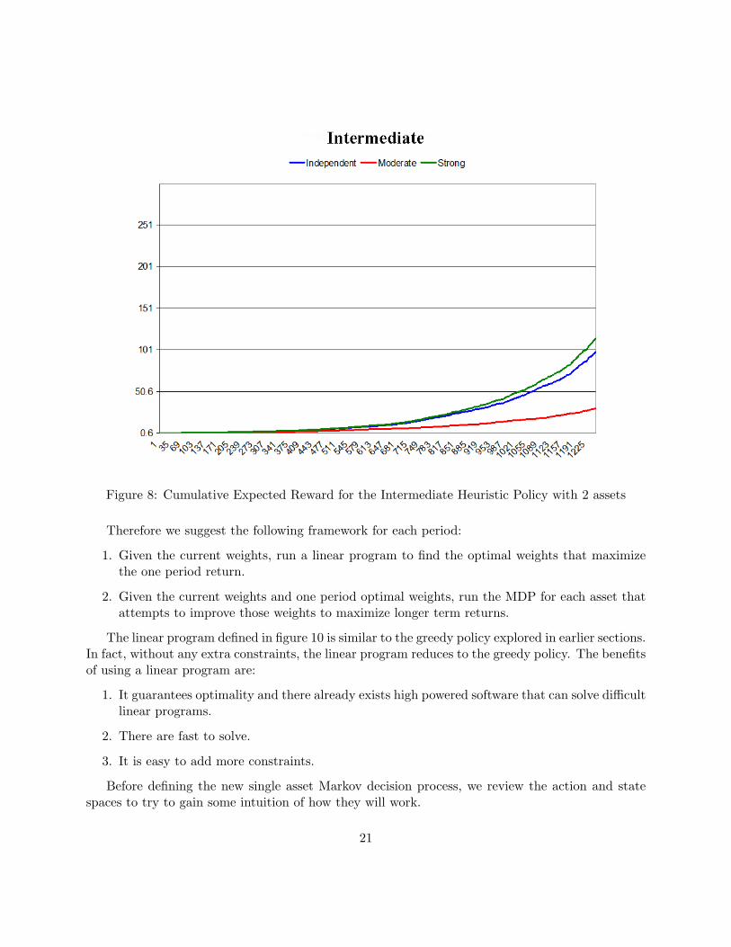
Figure 8: Cumulative Expected Reward for the Intermediate Heuristic Policy with 2 assets

Therefore we suggest the following framework for each period:

1. Given the current weights, run a linear program to find the optimal weights that maximizethe one period return.

2. Given the current weights and one period optimal weights, run the MDP for each asset thatattempts to improve those weights to maximize longer term returns.

The linear program defined in figure 10 is similar to the greedy policy explored in earlier sections.In fact, without any extra constraints, the linear program reduces to the greedy policy. The benefitsof using a linear program are:

1. It guarantees optimality and there already exists high powered software that can solve difficultlinear programs.

2. There are fast to solve.

3. It is easy to add more constraints.

Before defining the new single asset Markov decision process, we review the action and statespaces to try to gain some intuition of how they will work.

21

Figure 9: Cumulative Expected Reward for the Value Iteration Policy with 2 assets

5.1 Action Space

The action space is similar to a binary model. Given the current weight and the new weight fromthe linear program, the MDP can take the 6 following actions:

1. Accept the new weight given by the myopic optimization.

2. Increase the current weight by some constant amount.

3. Decrease the current weight by some constant amount.

4. Keep the weight from the previous day.

5. Increase the new weight by some constant amount.

6. Decrease the new weight by some constant amount.

The idea is the linear program gives a new weight that will maximize the one period return.However, if we can give enough information to our MDP, it should realize that by increasing the

22

Let w+i be the positive new weight assigned to asset i, w−

i be the negative new weight assigned toasset i and wi be the current weight of asset i. Let UB be the maximum weight allowed for onestock. Let α̂i be the expected return for stock i. Let ∆+

i be the positive change in weight for asseti and ∆−

i be the negative change in weight for asset i. Let c be the transactions cost constant.Then the linear program is defined as:

maximize

W∑i

w+i α̂i + w−

i α̂i − c(∆+i −∆−

i )

such that ∀i ∈W

w+i − wi ≤ UB

w−i − wi ≤ −UB

w+i ≥ 0

w−i ≤ 0

w+i −∆+

i ≤ wi

w−i −∆−

i ≥ wi

andW∑i

w+i − w−

i ≤ 1

Figure 10: The linear program used for the greedy policy

23

linear programs new weight, while it may be sub optimal for the next period, it will capture morereturn in the future.

For example, suppose the a asset with a current expected return of .05% will increase itsexpected return by .1% per day over the next two weeks. On the first day, the linear programonly sees the expected return was .05% today and .06% tomorrow, therefore may make a smallincrement in the weight. Similarly tomorrow it will make another small increment in the weight.However, the MDP may realize the asset is in a state that gives high expected return over the next2 weeks. Therefore, it may take the new weight from the linear program and adjust it upwardsmore, thereby capturing more of the return earlier on with less transactions costs.

5.2 State Space

We must consider what a meaningful state space for this new process would be. It needs to give asense of longer term movements in the asset, why the linear program assigned the new weight tothe asset, and any future movement of the asset so that we can make a decision that will maximizelonger term return. Therefore the state will actually contain a vector of asset features that try toencapsulate this information. Figure 11 lists the asset features contained in the new state. We thenprovide a description for each feature.

Figure 11: asset Features for the Single asset MDP

1. Expected return for the asset.

2. Standard deviation of the predicted expected return.

3. Current weight.

4. New weight assigned by the myopic optimization.

The expected return for the asset is the most importantThe current weight is the current percentage we’re holding of the asset. The new weight is what

the myopic optimization determined would maximize the one period portfolio return. These twoinputs are necessary to help the intertemporal decide whether to leave the current weight, take thenew weight or make its own modification to the weight.

The duration of the expected return of a particular asset describes how many days the expectedreturn will last. For example, one model may look at short term phenomenon while another modellooks at longer term behaviors. Both model may give an expected return of .1% per day, but if thelong term model expects that return to last for 30 days while the short term only expects 5 days,then the intertemporal optimization should prefer the long term signal to the short term signal.

The standard deviation of the expected return describes the models confidence in its prediction.If two assets have the same predicted return but the standard deviation on the first asset is muchhigher than the second, the intertemporal optimization should be more willing to invest in thesecond asset.

24

6 Defining the Constrained Markov Decision Process

The constrained MDP we define is for a single asset.

6.1 Decision Epochs:

The set of decision epochs is the same as the previous MDP.

6.2 States:

The state space S of the MDP consists of all possible combinations of asset features. If there are Ffeatures, then the MDP state is an F element vector where each element is the value of a feature.

6.3 Actions:

The action space A consists of the 4 actions described above. Each action leads to a new weight.Therefore if our current weight is wt, we take action at which gives us the new weight wt+1.

6.4 Transitions:

Each decision epoch, the MDP transitions to the same state or a new state, depending on thetransitions of the individual asset features.

6.5 Rewards:

The reward is the expected return from period t to t + 1 of the asset less transaction costs.

25

7 Solving an Optimal Policy for the Constrained MDP

To solve for the optimal policy, we will employ two different reinforcement learning algorithms thatuse a set of training data to approximate the value for each state. After we have trained themsufficiently, we can test them on an out of sample data set.

But first we make several important observations about the new Markov decision process. Weonly have a limited data set to learn a policy with, which means we will not see all the states intraining that will be encountered in the future. Furthermore, while there are not many features inthe state space, most of the features are in the real domain. As a result, we need to use functionapproximation to approximate the values of unseen states from the values of encountered states.Also, to simplify the process, we actually discretize the state space with some specified resolutionsuch that we have a discrete set of states. This addresses both the problem of limited training dataand real valued feature variables.

Secondly, there are only six actions available from any state but an infinite number of states(assuming some of the features are in the real domain). It is difficult to predict the probability oftomorrow’s state since it relies on the randomness of the economic model transition probabilitiesand the assignment of weights from the linear program. Therefore, if we can estimate the valueof a state action pair, we can easily choose the best action by just comparing the value for the 6actions with the current state and taking the maximum action. The value of state action pairs fora given policy π is written as Qπ(s, a).

The next two subsections describe the two algorithms we employ to derive our policy. Forboth learning algorithms we use function approximation to generalize the value of visited statesto those that haven’t been visited. Typical function approximators include neural networks, linearregression and k-nearest neighbor. We use the general idea of training an approximator, whichmeans giving the approximator a state/action value pair which it can use to generalize to unseenstates. In the case of a neural network, this implies feeding the state/action value pair through thenetwork to train the weights. In the case of k-nearest neighbor, it simply means storing that pairin memory.

In describing the two algorithms below, we use both psuedocode and descriptions given bySutton and Barto in their book Reinforcement Learning.

7.1 Off-Policy Q-Learning

Off-Policy Q-Learning uses a one step update to learn the values of each state. Therefore, once wehave visited a state and take an action, we update the value of that state/action pair by the rewardwe receive next period plus the maximum value for all actions taken at the new state. Therefore weuse bootstrapping by updating the estimated value of a state using the estimated values of otherstates.

Off-policy learning allows you to fully explore the state/action space because you can take anyrandom action. This is a major advantage as it allows you to visit much more states than if youhad to try to follow some specific policy. However, the disadvantage of one step updates is it maytake longer to converge because of the bootstrapping. Table 19 shows the learning algorithm inpsuedocode.

26

Off-Policy Q Learning(MDP, γ)

1. Initialize A(a) arbitrarily for all a

2. Initialize s and a

3. Initialize exploration policy π′

4. Repeat (for each episode):

(a) Observe r and s′

(b) Q(s, a)→ Q(s, a) + α[r + γ maxa′ Q(s′, a′)−Q(s, a)

](c) Train A(a) on input s and output Q(s, a)

(d) Choose a′ acoording to exploration policy π′

(e) s→ s′, a→ a′

Table 19: Q-learning using off-policy learning and on-line approximator updating

7.2 Sarsa(λ)

Sarsa is a learning algorithm that estimates Q(st, at) using the following update rule:

Q(st, at)← Q(st, at) + α[rt+1 + γQ(st+1, at+1)−Q(st, at)]. (12)

This rule uses every element of the quintuple of events, (st, at, rt+1, st+1, at+1), that make up atransition from one state action pair to the next. This quintuple give rise to the name Sarsa forthe algorithm.

The algorithm can also be implemented using eligibility traces as a Sarsa(λ) algorithm where0 ≤ λ ≤ 1 is a parameter than controls the number of steps to update a state action pairs value.If λ = 0, we do a 1 step update similar to dynamic program, while if λ = 1, we do a full episodeupdate similar to monte carlo learning. When λ is inbetween, it becomes a hybrid of the two. Letet(s, a) denote the trace for state-action pair s, a. Then the update can be written as

Qt+1(s, a) = Qt(s, a) + α∆tet(s, a)

for all s, a where

∆t = rt+1 + γQt(st+1, at+1)−Qt(st, at)

and

et(s, a) =

{γλet−1(s, a) + 1 if s = st and a = at,γλet−1(s, a) otherwise.

(13)

27

Sarsa(λ) is an on-policy algorithm, meaning it approximates Qπ(s, a), the action values for thecurrent policy, π, then improve the policy gradually based on the approximate values for the currentpolicy. The policy improvement can be done in many ways, such as using the ε-greedy policy withrespect to the current action-value estimates.

After each episode we will have a training set Q for the states and actions visited in the episode.We divide the training set by action into six subsets, each of which is used to train the neural networkfor that action. For the pseudocode below, A(a) refers to the approximator for action a. To getthe value Q(s, a), we pass the features for state s to the approximator A(a). The full algorithm isgiven in table 20.

The advantage with the online approach is it provides much more accurate updates since thereis less bootstrapping than the offline methods. However, you have to run many more iterations toget the same number of updates per state, therefore if time is an issue (which in our case it is) itmay not converge to good estimates.

sarsa(MDP, γ, λ)

1. Initialize Q(s, a) = 0 and e(s, a) = 0 for all s, a

2. Initialize A(a) arbitrarily for all a

3. Repeat (for each episode):

(a) Initialize s, a

(b) Repeat (for each step of episode):

i. Take action a, observe r, s′

ii. Choose a′ from s′ using current policy π

iii. ∆→ r + γQ(s′, a′)−Q(s, a)iv. e(s, a)→ e(s, a) + 1v. For all s, a where e(s, a) > 0:

A. ∆ = rt+1 + γQt(s′, a′)−Qt(st, at)B. Q(s, a)→ Q(s, a) + α∆e(s, a)C. e(s, a)→ γλe(s, a)

vi. s→ s′, a→ a′

(c) Train A(a) on the set of data points (s,Q(s, a)) for all s visited in the episode

Table 20: Sarsa(λ) using on-policy learning and trace weights for approximator training

7.3 Approximating the Values for each State

Unfortunately with four dimensions it is difficult to visualize the relationship between values andstates that both algorithms learn using training data. Therefore we reduced the dimensionality by

28

isolating two of the dimensions and average across the other dimensions for a given set of values.For example, we can get the average value for the set of states where the expected return is .005and the current weight is .01 by look at all states that satisfy these conditions and taking theaverage value. While it’s not perfectly accurate, it gives some intuition into the learning processand provides a sanity check to ensure the algorithms are running properly.

For each graph, the lower left corner shows negative expected returns and negative weights andthe upper right corner shows positive expected returns with positive weights. Therefore, you wouldexpect most mappings to have a diagonal ridge of positive values the tapers off towards the othertwo corners.

Figure 12 shows the value mappings for the online Sarsa learning algorithm. All the graphs lookgood except for the increment new weight action, which doesn’t appear to have learned any clearrelationship. It could be that the dimension reduction doesn’t translate well for this action, so thatthere are several very different states that are averaged together and cancel each other out. Also,the online sarsa takes longer to converge and therefore it’s possible we didn’t run it for enoughiterations to converge to clear values.

Figure 13 gives the value mappings for the offline Q-Learning algorithm. These graphs all lookgood. It is interesting to note the small space explored for the two increment actions. This mayhave been a function of the random policy followed which didn’t give enough increment actions.

7.4 Results

We used 3 different policies and evaluated them over 252 days of market data during 2004. The firstpolicy, the greedy policy, just takes the new weight given by the linear program every period. Thesecond policy, the off-line Q-Learning policy, chooses the action that maximizes expected returnusing approximators trained from the off-line Q-Learning algorithm. The final policy, the on-lineSarsa policy, chooses the aciton that maximizes the expected return using approximators trainedfrom the on-line Sarsa policy.

We chose a k-nearest neighbor method for function approximation. Gordon suggests usingk-nearest neighbor instead of neural network or linear regression for large state spaces since k-nearest neighbor approximation cannot produce anything that hasn’t already been seen. Since wewere already concerned that the learning algorithms weren’t being trained enough, using a neuralnetwork or linear regression would add another layer of uncertainty in the approximation process.

We used a universe of 2000 stocks and added several constraints to keep a balanced portfolio.We were only allowed to invest .5% in any one stock and had to be equally invested in each sector.We trained both learning algorithms using data from 2001-2003. The cumulative return for the 3policies is given in figure 14.

We were surprised that the greedy algorithm outperformed both learning algorithms. There aremany different possible reasons for this behavior. The first is that the learning algorithms neededmore iterations to more accurately estimate the state/action value mapping. We used a somewhatcoarse discretization so that the learning algorithms could update each state more times. However,perhaps the grid was too coarse which combined with k-nearest neighbor approximation failed togive good estimates for values.

29

Perhaps k-nearest neighbor failed to generalize well and a neural network or some other approx-imator would give better function approximation. Especially if the relationship is very nonlinear,k-nearest neighbor tends to smooth these nonlinear features and therefore would give a poor esti-mate.

Bent and Van Hentenryck note a Markov decision process may be too complicated a model forthis type of problem since the uncertainty in the system does not depend on the action. MDP’sare useful because the uncertainty in the system is a function of both the states and the actions.However, in our case, the uncertainty in the system is completely a function of the Markov processfor each stock. Regardless of the actions we take to buy or sell assets, each asset will follow itsown Markov process independent of our actions. Therefore the MDP model we used may be toocomplicated, especially for such a large search space. The MDP model would be better suited toa market condition where the action to buy or sell a stock affects its movement. In this case, thesystem becomes much more complicated and the uncertainty stems from both the Markov processof the asset and the action to buy or sell.

Finally, by breaking the portfolio MDP into several MDPs, one for each asset, perhaps thereisn’t enough communication between components so that suboptimal decisions are made. Eachasset MDP makes its own decision using information contained in the state features. Perhapsexpanding the number of features we use to describe the state would improve this communicationand each MDP could make a better decision for the portfolio. These features could include:

1. Duration of the expected return predicted by the Markov process.

2. Stability of the weight assigned by the linear program.

3. Tightness of the weight against constraints imposed on the optimization.

4. The old and new weights of stocks correlated with this stock.

However, each new feature adds a dimension to the state space and compounds the problem offunction approximation so there is a clear tradeoff.

8 Conclusion

With a small state space, its clear a Markov decision process is a good model for the portfolioproblem that can produce an optimal policy. However, the weakness of Markov decision processesis its dependence on estimating values throughout the state space. When we moved to a largerstate space, the well known techniques like value iteration could not be used.

We introduced two algorithms using reinforcement learning combined with linear programmingto try to cope with the large state space. We also simplified the model by posing each stock as itsown Markov decision process, rather than trying to model the entire portfolio as an MDP. Thesetwo algorithms failed to improve on the simple greedy approach of using the weights given by thelinear program.

30

Although the two algorithms we implemented failed to beat the greedy algorithm, with moreresearch this framework could still be used. There were several implementation specific decisionsmade that could have affected performance. We suggested a few in our analysis in the last section.

31

9 References

MARTIN L. PUTERMAN, 1994, ”Markov Decision Processes”, John Wiley & Sons, New York

RICHARD S. SUTTON and ANDREW G BARTO, 1998, ”Reinforcement Learning”, The MITPress, Cambridge, Massachusetts

GEOFFREY J. GORDON, 2005, ”Stable Function Approximation in Dynamic Programming”

RUSSELL BENT and PASCAL VAN HENTENRYCK, 2005, ”Online Stochastic OptimizationWithout Distributions”

32

Figure 12: State/Action Value Mapping for each action computed using on-line Sarsa algorithm33

Figure 13: State/Action Value Mapping for each action computed using off-line Q-Learning algo-rithm

34

Figure 14: Cumulative portfolio return achieved by following the 3 different policies. The greedyalgorithm outperforms both learning algorithms.

35