Using modern hardware for effectivelarge data visualization

Martin Florek

2006

Using modern hardware for effectivelarge data visualization

diploma thesis

Martin Florek

Univerzita Komenského v Bratislave

Fakulta Matematiky, Fyziky a Informatiky

Katedra Aplikovanej Informatiky

computer graphics

supervisor: Mgr. Matej Novotný

Bratislava 2006

Declaration on word of honour

I hereby declare, that the research and results presented in this thesis

were conducted by myself using the mentioned literature and advices of my

supervisors.

i

Abstract

The actual technology behind visualization is meant to provide fast and

accurate rendering results and thus to support the exploratory data anal-

ysis in an information visualization environment. A crucial element in the

exploratory process is overall interactivity, especially when dealing with mul-

tidimensional data. However, with the ever growing volume of nowadays

data, a fast and interactive display easily becomes static, giving only slow or

even none actual interaction feedback.

The technical improvements presented in this work are oriented on using

modern graphics hardware to modify the standard rendering process of a

popular information visualization display, the parallel coordinates and scat-

terplot, in an interaction-oriented way. By intelligently using the advanced

features of the now common hardware we achieved great improvement over

standard CPU-oriented implementations in terms of both speed and visual

quality.

ii

Contents

Declaration on word of honor . . . . . . . . . . . . . . . . . . . . . i

Abstract . . . . . . . . . . . . . . . . . . . . . . . . . . . . . . . . . ii

1 Introduction 1

1.1 Interaction . . . . . . . . . . . . . . . . . . . . . . . . . . . . . 2

1.2 Parallel Coordinates . . . . . . . . . . . . . . . . . . . . . . . 3

1.3 Scatterplot . . . . . . . . . . . . . . . . . . . . . . . . . . . . . 5

1.4 Identifying the problem . . . . . . . . . . . . . . . . . . . . . . 6

2 State of the art report 8

2.1 Scientific Visualization . . . . . . . . . . . . . . . . . . . . . . 9

2.2 Medical Visualization . . . . . . . . . . . . . . . . . . . . . . . 10

2.3 Information Visualization . . . . . . . . . . . . . . . . . . . . 11

2.4 Other rendering . . . . . . . . . . . . . . . . . . . . . . . . . . 12

2.5 Difference between rendering for InfoVis and other applications 12

2.6 Hardware acceleration in information visualization . . . . . . . 14

3 Software specification 18

3.1 Introduction . . . . . . . . . . . . . . . . . . . . . . . . . . . . 18

3.2 Overall Description . . . . . . . . . . . . . . . . . . . . . . . . 18

3.3 Main system features . . . . . . . . . . . . . . . . . . . . . . . 19

iii

3.4 Technologies . . . . . . . . . . . . . . . . . . . . . . . . . . . . 20

3.5 System requirements . . . . . . . . . . . . . . . . . . . . . . . 21

3.6 Other Nonfunctional Requirements . . . . . . . . . . . . . . . 21

4 Implementation 23

4.1 Incorporating the GPU . . . . . . . . . . . . . . . . . . . . . . 24

4.1.1 GPU vs. CPU . . . . . . . . . . . . . . . . . . . . . . . 25

4.2 Parallel Coordinates . . . . . . . . . . . . . . . . . . . . . . . 26

4.2.1 Immediate mode . . . . . . . . . . . . . . . . . . . . . 26

4.2.2 Vertex arrays and vertex programs . . . . . . . . . . . 27

4.2.3 Performance cap hit . . . . . . . . . . . . . . . . . . . 28

4.2.4 Experiments . . . . . . . . . . . . . . . . . . . . . . . . 28

4.2.5 Improving visuals . . . . . . . . . . . . . . . . . . . . . 29

4.2.6 Conclusions . . . . . . . . . . . . . . . . . . . . . . . . 34

4.3 Scatterplot . . . . . . . . . . . . . . . . . . . . . . . . . . . . . 34

4.3.1 Immediate mode . . . . . . . . . . . . . . . . . . . . . 34

4.3.2 Vertex arrays and vertex programs . . . . . . . . . . . 34

4.3.3 Fish-eye . . . . . . . . . . . . . . . . . . . . . . . . . . 35

4.3.4 Conclusions . . . . . . . . . . . . . . . . . . . . . . . . 36

4.4 Sorting the data . . . . . . . . . . . . . . . . . . . . . . . . . . 36

4.5 Histogram . . . . . . . . . . . . . . . . . . . . . . . . . . . . . 37

5 Summary 38

6 Abstrakt v Slovenčine 42

iv

Chapter 1

Introduction

Information visualization1 uses graphical representation of data to sup-

port and accomplish important tasks like decision making, data exploration

or analysis. Compared to scientific visualization, where the data usually

contains an underlying spatial geometry, the data in the information visu-

alization domain are often highly multidimensional and usually have no a

priori structure or layout.

The motivation for graphical depiction of data is the wide information

highway that is provided to humans through the sense of vision. Even the

most complicated structures and information can (using a proper visual-

ization) be communicated between the man and the machine. Numerous

projection methods and graphical metaphors were designed in the field of in-

formation visualization [1] [2] [3]. However, the fully comprehensive mental

image of a multidimensional information is only built through the means of

user interaction [4].

1InfoVis

1

Our work is oriented on technical improvements. First we will show you

basic InfoVis techniques for displaying the data and then we will reveal our

implementations, how to make those displays fast. Therefore the most im-

portant chapter is the Implementation chapter.

1.1 Interaction

By performing direct manipulation inside the display, through observing

the data from different aspects and under different conditions the users im-

merse themselves in the data. If the display reacts within a fraction of a

second (say 100 ms) the user gets the feeling of actually touching the data

[5] and can better understand the intrinsic structures of the observed space

or model.

In an information visualization environment the interaction provides (a-

mong others) an access to changing parameters of the visualization and to

selecting and emphasizing areas of interest. But if the actual time to refresh

the display after such an action takes too long for the user to notice the dif-

ference or to perceive the fluent changes the interaction suffers greatly. This

happens for large data cases in combination with demanding visualization

techniques. Parallel coordinates are an example of a popular and widely ac-

claimed visualization method that faces severe problems when large data is

observed.

2

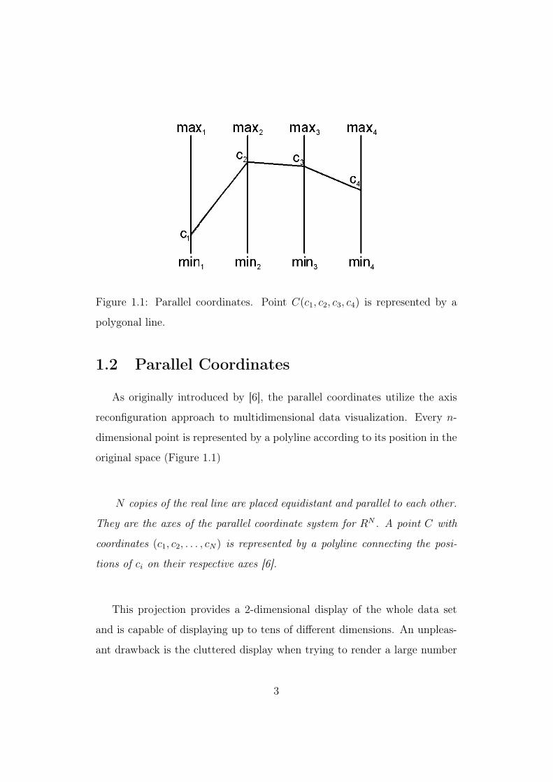
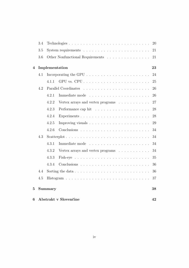
Figure 1.1: Parallel coordinates. Point C(c1, c2, c3, c4) is represented by a

polygonal line.

1.2 Parallel Coordinates

As originally introduced by [6], the parallel coordinates utilize the axis

reconfiguration approach to multidimensional data visualization. Every n-

dimensional point is represented by a polyline according to its position in the

original space (Figure 1.1)

N copies of the real line are placed equidistant and parallel to each other.

They are the axes of the parallel coordinate system for RN . A point C with

coordinates (c1, c2, . . . , cN) is represented by a polyline connecting the posi-

tions of ci on their respective axes [6].

This projection provides a 2-dimensional display of the whole data set

and is capable of displaying up to tens of different dimensions. An unpleas-

ant drawback is the cluttered display when trying to render a large number

3

of samples (Figure 1.2). Interaction and even mere understanding of such a

display is complicated.

Figure 1.2: cluttered parallel coordinates view

A common graphical feature of the parallel coordinates is semi-transpa-

rency of the polylines. It gives better understanding of an over plotted display

by steering the visual importance toward the dense areas where multiple semi-

transparent lines overlap. However this improvement has certain limitations

due to the dynamic range of the alpha channel [7]. In addition to that the

use of transparency and color blending introduces a significant performance

issue.

4

1.3 Scatterplot

Figure 1.3: Scatterplot display example

Scatterplot is another popular method for information visualization.

Each sample is represented by a dot on a graph where vertical and horizontal

axes represent two chosen dimensions (Figure 1.3). Resulting pattern shows

relation between them.

Also in scatterplot display, when rendering large amount of samples, the

display can easily get cluttered. In scatterplot display we do not use blending

5

to solve this issue, but we use fish-eye projection to achieve magnifying lens

effect [8].

1.4 Identifying the problem

We try to make InfoVis displays more interactive, then they are today.

We try to maximize the performance of rendering. So we need to balance

the CPU vs. GPU load. We have to identify which parts of the system are

CPU, GPU, RAM and VRAM intensive.

Some datasets are RAM intensive because they are vast and have many

dimensions, sometime hundreds. So we must carefully choose data structures

to hold the data, so we can effectively work with them.

If we want to get the maximum interactivity, we must render as fast as

possible. That means, combining several methods, such as using shaders and

storing the data in VRAM2. Rendering of the data will become GPU inten-

sive with large datasets, so we will try several techniques of rendering and

choose the best one.

The CPU intensive part is the filtering. When user is selecting the data

we must quickly change the degree of interest (DOI), which is not so trivial

to make it fast, when making logical operations between different selections

and of course when we work with hundreds of thousands of records or even

more. In many cases (usually for good and informative rendering output) we2Actually, storing data in VRAM did not yield any performance boost.

6

need to sort the data according to DOI, which can not be done with simple

quicksort, because the data is always almost sorted containing mainly zeros

and ones.

7

Chapter 2

State of the art report

Visualization is a subset of computer graphics and image processing. It

can be divided in categories such as Scientific Visualization, Medical Visual-

ization, Information Visualization, Flow Visualization etc.

In Medical Visualization, hardware acceleration has been used for several

years now. It is mainly because, they visualize big volumetric datasets, of

which visualization on CPU was very slow. GPU provides enough power to

render volumes at interactive speed1.

Information Visualization systems of past did not need HW acceleration,

because they were usually displaying only small data, thus rendering was

interactive. But by the end of the 20th century the fast development of data

acquisition and data storage technology cause the data sets to grow in size.

InfoVis systems became slow and work became inconvenient because of lack

of interactivity.1single channel volumes up to 512×512×512 on cards with at least 256MB of VRAM.

And 4 channels on cards with at least 640MB of VRAM (3Dlabs Wildcat Realizm 800)

8

2.1 Scientific Visualization

SciVis is a graphical representation of data, to understand it and gain

insight into it. It is mainly aimed towards visualizing large spatial data such

as those from physical simulations or from observation of real world phenom-

ena. Such data can consist of millions of entries.

SciVis also deals with visualization of computational fluid dynamics, finite

element analysis, meteorology, data fusion etc. Example of SciVis is shown

on Figure 2.1.

Figure 2.1: SciVis example

from The AVS Workbook c©Ken Flurchick 2003

Even though complicated in its dimensionality and large in its size, the

data that is the object of scientific visualization often contain some kind of

underlying geometry. This is given by the space of the modeled environment –

e.g. a chamber inside an engine, geographical whereabouts of a thunderstorm,

interior of a building etc.

9

2.2 Medical Visualization

Medical Visualization is mainly about volume rendering. Data is pro-

vided from CT and MR scans in form of slices, which represents the whole

head, for example.

In volumetric rendering there are several methods like shear warp or di-

rect volume rendering with 3D textures. Shear warp is unimportant for our

purposes, so for further study of this method see [9].

Figure 2.2: direct volume rendering

http://www.crs4.it/vic/activities/direct-volume-rendering/

One of the direct volume rendering techniques is texture mapping. Gelder

et. al. implemented 3D texture mapping which produces a high quality 3D

image at interactive rendering speeds [10]. Direct volume rendering allows

users to view and interact in real-time with the volume. Users can render

perspective views of 3D voxel data and make arbitrary cuts. This technique

10

can be used for our purposes, such as visualizing 3D scatterplots2.

2.3 Information Visualization

Information Visualization combines several methods and brings some new

as it works with more general data without any particular geometry.

Two of the most popular InfoVis techniques are Scatterplot and Parallel

Coordinates 2.3. Each of these methods is described in more detail in later

chapters.

Figure 2.3: parallel coordinates by Martin Florek

In visualization, there is one very important aspect. That is, that user

can have multiple views on the same data [11]. In every view, user can

choose different style of visualization. Also linking between these views is

very important. That means, that if user changes data (make selection, add2for more complex 3D scatterplots, voxel representation is insufficient

11

to selection, etc.) in one view, all other views are affected.

2.4 Other rendering

Other rendering methods are rendering polygons, point clouds and glyphs.

Examples of these methods can be seen in Figures 2.4 and 2.5.

For rendering of huge amounts of polygons and/or lines and/or points we

will use modern graphics card with full OpenGL 2.0 support and support

of EXT_framebuffer_object extension. Todays gaming cards, which can be

found inside general purpose PCs, can render hundreds of millions of polygons

per second. But gaming cards acceleration of primitives such as points and

lines (which we will render the most) is not so good, because games don’t need

them. Professional CAD graphics cards has excellent acceleration for lines

and points, so our system would certainly run better on such hardware, but

it won’t be necessary. The reason for not using CAD cards is their big price

not worth their performance and only the newest and the most expensive

ones support advanced features such as high definition textures and others.

2.5 Difference between rendering for InfoVis

and other applications

Rendering for InfoVis system is completely different then rendering for

other applications such as games and CAD systems.

Rendering for games inclines toward detailed polygonal models, cutting-

edge graphic effects and in general, toward eye-candy. This is the complete

opposite of rendering in InfoVis systems. This does not incline to eye-candy,

12

Figure 2.4: Stanford bunny

Figure 2.5: point clouds Stanford bunny

but toward clarity, visibility, occlusion.

CAD systems are oriented on rendering a mixture of polygons, lines a

and points, which is closer to InfoVis rendering then games rendering, but it

is still a whole lot different.

13

But all have one common thing, they are fast or should be fast. So we

will learn from both styles (games and CAD) and implement usable things

into our system. We will take just the performance part, not the eye-candy

one.

2.6 Hardware acceleration in information visu-

alization

There is very little or almost no related work on making HW accelerated

InfoVis system. And why is that? It is because that ten years ago research

was dedicated to making things clear and to make them interactive. It was

believed that in few years there will be fast enough computers to make the

systems interactive. Now years have passed and the interactivity is still poor

as it was in middle nineties3. In that time data become larger, then those

days systems can handle in interactive way. We want to interact in real-time

with displayed informations, so focus is changing toward interaction.

One focus of our research is to use modern graphics card for effective

displaying of large datasets. So the rendering of all display-critical parts will

be accelerated with graphics card on general purpose PC.

Here are some examples from current InfoVis applications, such as Xmdv

(Figure 2.6), which is a free tool popular in academic spheres.

3before, those systems were fast enough, because data were small

14

Figure 2.6: XmdvTool

There is also SimVis (Figure 2.7) which is developed in VRVis Research

Center in Vienna, Austria. This tool is an interactive visual analysis system,

which received many acknowledgments at scientific conferences.

Also known, is an open source project The InfoVis Toolkit (Figure 2.8).

This is just framework written in Java to ease the development of InfoVis

applications.

15

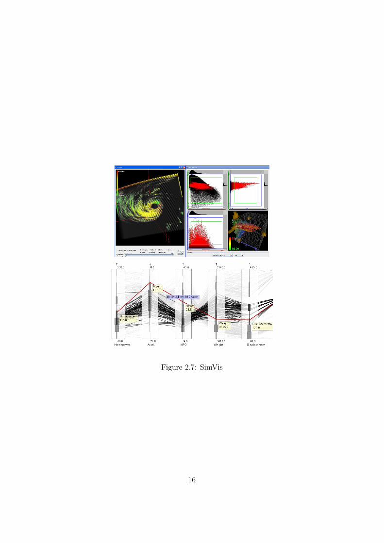
Figure 2.7: SimVis

16

Figure 2.8: The InfoVis Toolkit

17

Chapter 3

Software specification

3.1 Introduction

The purpose of our system is to present our techniques of fast rendering

of InfoVis views. It should not replace older applications, but just show the

way to go (and ways not to go) if one wants interactive views.

3.2 Overall Description

We gave our system codename ffVis. It is much faster then todays systems

as Xmdv [12] and therefore more interactive. User can interact in real-time

in almost all cases, except of really big datasets.

Our system contains one main window, where user is able to load data.

After loading the data, the main window shows information about the num-

ber of dimensions, number of records, etc.. From the main window user can

open new view windows, where he/she can view the actual data and explore

it. Views contain the most common styles as parallel coordinates and scat-

18

terplot.

In the view windows (user is able to open as many view windows as neces-

sary) user can choose from viewing style and will be able to perform different

actions.

User can interact with the system in various phases as can be seen on 3.1.

Figure 3.1: interaction phases

3.3 Main system features

• multiple views

• linking multiple views

• brushing (AND, OR, NOT)

• constraints, change viewing intervals

• text description of dimensions

• in scatterplot view, user can select channels

19

• and flip channels

• and use fish-eye with adjustable radius and distortion

• in parallel coordinates it is able to add/remove axes,

• exchange of axes and

• flipping axes intervals,

• then selection on axes

• and coloring according to axis and degree of interest (DOI)

• user has full control over colors, that mean that user can customize

every color in the system

• user can use different transfer functions on density values

3.4 Technologies

We have decided to program our system in language C++ with OpenGL

for hardware acceleration of graphics. It was developed on a Microsoft Win-

dows platform.

We were deciding between various libraries for graphical user interface. In

particular we were deciding between MFC, .NET Framework 2 and wxWid-

gets. MFC was rejected because of no chance of porting to other platforms

other then Microsoft Windows and more complicated work on making GUI

then .NET Framework. wxWidgets was refused because of no easy-to-use

GUI designer.

20

Finally we have chosen the Microsoft .NET Framework 2. Because of ease

of designing GUI, the speed of GUI (GUI part of .NET Framework 2 is nearly

as fast as MFC or WinApi) and because in future it will be supported on

UNIX and Linux platforms. Thanks to project MONO (http://www.mono-

project.com/) for developing the .NET Framework port for UNIX and Linux.

And of course, the Microsoft Visual C++ 2005 Express Edition is for free.

We use GLEW extensions loading library for loading OpenGL extensions

with multiple contexts support1.

3.5 System requirements

Minimum system requirements are a PC with Windows XP with in-

stalled .NET Framework 2 2 and a graphics card with full GLSL support

(we need branching in fragment program) and with floating point blending

with proper drivers. Application also needs to support of OpenGL’s ex-

tension EXT_frame-buffer_object. nVidia GeForce 66003 and up and ATi

Radeon X10004 and up.

3.6 Other Nonfunctional Requirements

Our system is fast and the interaction is possible in real-time. Our system

is robust, what means that it won’t crash on unexpected cases, like user1multiple contexts are necessary for support of multiple view2without .NET Framework 2 the app will not start, it will crash on start attempt3GF 6200 does not support fp16 blending4we did not havy any to test on, but it should run

21

making something illogical, etc..

22

Chapter 4

Implementation

This is the most important chapter of this diploma thesis. It shows tech-

nical details of our implementations.

As mentioned in software specification chapter, our system is written

in C++ language, with the use of OpenGL for hardware acceleration of

graphics. Our system can read data in okc format, which is also used by the

Xmdv tool and is easy to implement.

Data of arbitrary size1 can be read-in, limited only by system memory.

We tested our system with data up to 150.000 records with 5 dimensions,

and achieved speeds were acceptable.

23

Figure 4.1: The same data containing 150.000 samples. Rendering the par-

allel coordinates plot using the popular free visualization tool Xmdv took

more than 20 seconds (left). Our implementation (right) of parallel coordi-

nates works interactively with the data.

4.1 Incorporating the GPU

Even though the advanced rendering and processing capabilities of nowadays

graphics cards are originally oriented on producing realistic images and spe-

cial effects in real time, much of this functionality can also be used to improve

information visualization.

The current graphics hardware with its wide range of advanced processing

features provides a promising solution to improve the interactivity of large

data visualization. Scientific visualization with numerous volumetric render-

ing approaches and applications uses the graphics hardware for quite a long

time now.1we have limitation of 128 dimensions because of sorting the data, there is no limitation

on number of records

24

Figure 4.2: A simple visualization pipeline. In its original form (top) the

CPU has to perform much more operations than now (bottom).

However in information visualization domain, the actual technological

improvements using the GPU receive little attention. In contrast to that, this

project focuses on accelerating parallel coordinates and scatterplot using the

GPU in order to produce a display that is capable of displaying data sets with

tens or hundreds of thousand samples while still providing fast interaction

options to the user (Figure 4.1)

4.1.1 GPU vs. CPU

The parallel coordinates projection has a well defined and simple geomet-

ric nature which nicely favors GPU over CPU. With the powerful geometry

processing units and parallel pipelines of the GPU many sub-tasks of the vi-

sualization process can be transferred to the graphics hardware (Figure 4.2.)

The comparison of using CPU and GPU to do visualization tasks is il-

25

lustrated in Figure 4.1. The left picture shows a rendition by the Xmdv vi-

sualization tool [12] that took 20 seconds to accomplish. Our GPU-powered

solution (right) performs about 60 times faster.

4.2 Parallel Coordinates

In this section we will describe our implementations of a hardware accel-

erated parallel coordinates display and we will show our experimental results.

4.2.1 Immediate mode

Our first implementation was naive immediate mode, where the screen

coordinates are computed on CPU and each record (line strip) is send to the

GPU vertex by vertex:

for (each record) {

// compute color according to DOI

glColor3f(color);

glBegin(GL_LINE_STRIP);

for (every axis) {

// compute vertex coordinates from zoom range and window height

glVertex3f(coordinates);

}

glEnd();

}

26

This implementation runs fine. On smaller data sets the rendering of

parallel coordinates is instant. On larger data sets, this method was clearly

CPU bound, because of millions of function calls per frame and too many

mathematical operations.

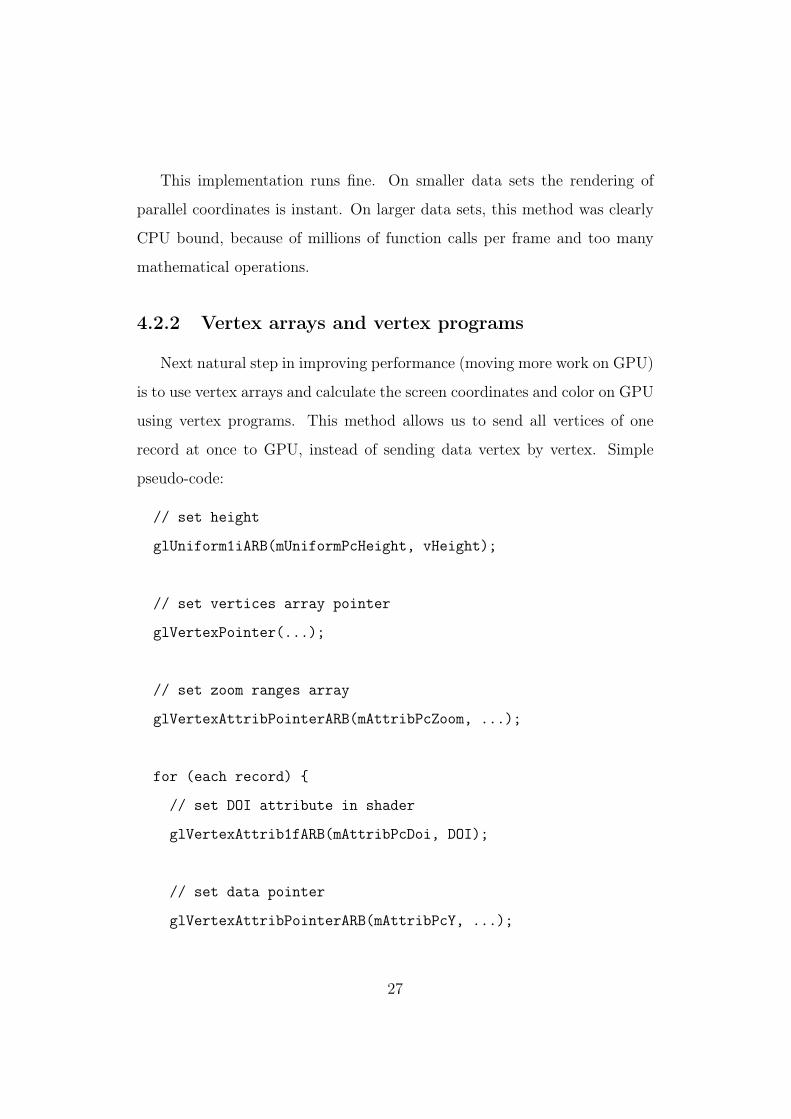
4.2.2 Vertex arrays and vertex programs

Next natural step in improving performance (moving more work on GPU)

is to use vertex arrays and calculate the screen coordinates and color on GPU

using vertex programs. This method allows us to send all vertices of one

record at once to GPU, instead of sending data vertex by vertex. Simple

pseudo-code:

// set height

glUniform1iARB(mUniformPcHeight, vHeight);

// set vertices array pointer

glVertexPointer(...);

// set zoom ranges array

glVertexAttribPointerARB(mAttribPcZoom, ...);

for (each record) {

// set DOI attribute in shader

glVertexAttrib1fARB(mAttribPcDoi, DOI);

// set data pointer

glVertexAttribPointerARB(mAttribPcY, ...);

27

// render

glDrawElements(GL_LINE_STRIP, ...);

}

We heavily reduced the CPU load, because we moved all the math onto

the GPU, which is faster and processes more vertices in parallel. But the

function call number was still too high on larger data sets.

Next simple step in reducing number of function calls (and of course

reducing CPU load on large data sets) was to pack multiple records to one,

instead of glDrawElements we use glMultiDrawElements. This method need

some data preprocessing before each batch, but it is just simple data copying,

so it is very cheap. We reduced function call number several times. From

now on, our implementation is not CPU bound.

4.2.3 Performance cap hit

After trying several other methods (which we will discuss in next sub-

section) and with help of nVidia’s instrumented driver and gDEBugger [13]

we reached the conclusion, that our current implementation is rasterization

bound, and only more powerful graphics card will improve performance.

gDEBugger showed, that graphics card spends 98% of the time on raster

operations.

4.2.4 Experiments

Here we will present other methods, which did not improve performance

and were abandoned.

28

ASM vs. glSlang

We tried both version of vertex programs, the assembler ones and also

the high level glSlang. There was no difference in rendering speed.

VBO

We also tried to store all the data in graphics memory, using vertex buffer

objects (VBO)2. We did no observe any speed difference between storing data

in VRAM and regular RAM so we abandoned this path.

Using quads

It is known, that quads should be better accelerated then lines on gaming

cards. So we tried to render degenerated quads instead of lines. The quads

method did not bring any performance gain, only the visual side was worse.

This method was also abandoned.

4.2.5 Improving visuals

Blending

A common feature of a parallel coordinates display is the use of semi-

transparent polylines to clear up an over plotted display. The resulting

frequency-like graphical representation gives more information than a clut-

tered and indistinct visualization without the transparency. Dense areas are

emphasized by higher opacity values in contrast to the sparsely populated

areas which are less saturated (Figure 4.3)

2150.000 records with 5 dimensions take around 4MB of RAM

29

Figure 4.3: Transparency and alpha blending turn a cluttered and indistinct

display (left) into a much clearer shape (right).

Introducing transparency to the visualization brings the drawback of re-

duced performance. The cause is the large amount of overlapping fragments

created by numerous lines and therefore many raster operations.

Even with simple blending the performance is reduced by up to 70 percent

in an average parallel coordinates display. This could easily make a visual-

ization incapable of interactive response. We used stencil test performed on

the GPU to eliminate a significant number of fragments thus gaining some

of the lost performance.

The resulting visualization using the stencil test operates 2.5 times faster

than without the stencil test, reducing the 70 percent performance penalty

to less than 25 with the alpha blending on (Figure 4.4).

30

Figure 4.4: Comparison of blending performance on around 50k records

Figure 4.5: Cluttered view with simple blending.

Advanced blending and FBO

Sometimes simple linear blending is not enough to make display more

clear. Especially for large data sets, where can huge overdraw occur (Figure

4.5). We want arbitrary blending e.g. logarithmic, or even arbitrary opacity

mapping function.

31

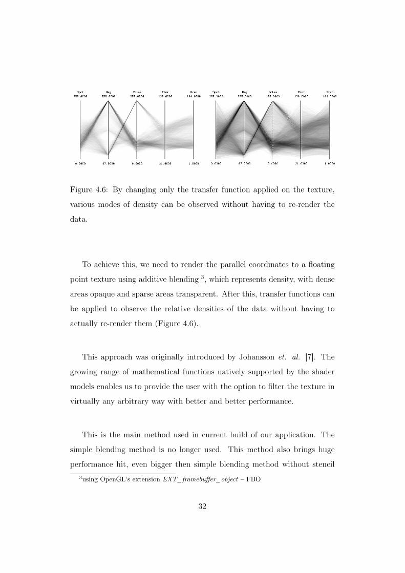
Figure 4.6: By changing only the transfer function applied on the texture,

various modes of density can be observed without having to re-render the

data.

To achieve this, we need to render the parallel coordinates to a floating

point texture using additive blending 3, which represents density, with dense

areas opaque and sparse areas transparent. After this, transfer functions can

be applied to observe the relative densities of the data without having to

actually re-render them (Figure 4.6).

This approach was originally introduced by Johansson et. al. [7]. The

growing range of mathematical functions natively supported by the shader

models enables us to provide the user with the option to filter the texture in

virtually any arbitrary way with better and better performance.

This is the main method used in current build of our application. The

simple blending method is no longer used. This method also brings huge

performance hit, even bigger then simple blending method without stencil3using OpenGL’s extension EXT_framebuffer_object – FBO

32

testing4. This is mainly because we use floating point textures to get more

then 255 density levels5. Our current implementation supports up to 4095.

This is limitation of fp16 blending, fp32 blending is currently unsupported

on today gaming graphic cards6.

Computing maximum value from density texture

Maximum value is needed to properly apply transfer functions. Without

it, we won’t be able to normalize density values. Monitor can display RGB

values in intervals from 0 to 1. All values above 1 are clamped to 1, so all in-

formation is lost. Therefore we compute maximum value of density texture,

then normalize each value and after that we apply transfer function to that

normalized value.

To compute maximum value from density texture, we originally imple-

mented simple, but slow method, where we read back all the texture values to

RAM and iterate through all values and find the max value. The slowest part

is the read back and on larger textures the time to compute the maximum

value was long. So we implemented another simple method called reductions,

mentioned in [14], which runs on GPU and only the final maximum value is

read back to RAM. We need it for other computations on CPU, otherwise we

would store it in 1× 1 texture, to speed the process an additional bit more.

On our surprise the GPU versions through reductions did not yield any

performance boost.4FPS dropped from 10 to 2. with simple method it was 3 FPS an same data5255 levels can be achieved with standard 8-bit textures6This limitation can be pushed with simple trick presented in [7]

33

4.2.6 Conclusions

Our current HW implementation7 renders 150.000 records with 5 dimen-

sions in 400× 400 sized window in 500 milliseconds with advanced blending

on. Using CPU version, without any blending, we achieve rendering time

of around 1000 milliseconds. Current HW implementation is rasterization

bound, so only a more powerful graphics card can improve performance.

4.3 Scatterplot

Here we will describe our implementations of a hardware accelerated scat-

terplot display.

4.3.1 Immediate mode

As with parallel coordinates, in scatterplot we implemented immediate

mode also as the first. The screen coordinates and color are computed on

CPU and each record (point) is send to the GPU vertex by vertex. This

implementation performed very well, even for large data sets. In spite of

good performance we were hoping for better performance.

4.3.2 Vertex arrays and vertex programs

With vertex arrays and vertex programs we need only one function call

to send all the data to GPU. Performance did improve several times on large

data sets. We achieve up to 300 FPS when rendering 150.000 elements in

arbitrary sized window.8 This is due to fact, that only small point is rendered7we use glSlang shaders, not ASM8even 3.000× 1.000!

34

for each record, thus generating smaller amount of fragments compared to

parallel coordinates display.

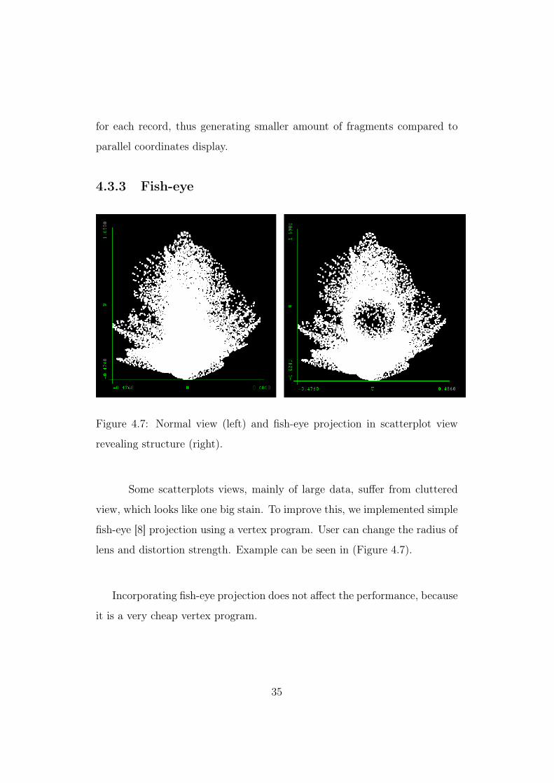
4.3.3 Fish-eye

Figure 4.7: Normal view (left) and fish-eye projection in scatterplot view

revealing structure (right).

Some scatterplots views, mainly of large data, suffer from cluttered

view, which looks like one big stain. To improve this, we implemented simple

fish-eye [8] projection using a vertex program. User can change the radius of

lens and distortion strength. Example can be seen in (Figure 4.7).

Incorporating fish-eye projection does not affect the performance, because

it is a very cheap vertex program.

35

4.3.4 Conclusions

Our scatterplot display, which is using simple vertex arrays9 and vertex

programs, is instant on all tested datasets (up to 150.000 records with 5

dimensions).

4.4 Sorting the data

Very important part of our system is fast sorting of data according to DOI

after each change to selection. This is needed to easily render data in cor-

rect way. Implementation in C of quicksort algorithm gave very poor results,

because the data is almost always sorted. So we used introsort implemented

in STL10. Using STL’s sort on our data structure was a bit difficult, but we

succeeded11. This difficulties also brings constraint of max 128 dimension on

input data 12.

On our test machine, sorting with C’s qsort function of 150.000 nearly

sorted records lasted for up to 1 minute! Thus making the display useless.

STL’s implementation of introsort sorts the same data in 20 milliseconds.9we do not store data in video RAM

10Standard Template Library11look into complicatedsort.h and .cpp files12we could provide some more, but the final application becomes larger, the compila-

tion time is too long, and there is also limitation in compiler for this method and more

dimensions are not necessary for major data sets

36

4.5 Histogram

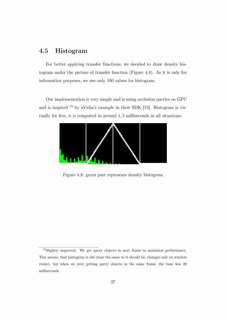
For better applying transfer functions, we decided to draw density his-

togram under the picture of transfer function (Figure 4.8). As it is only for

information purposes, we use only 100 values for histogram.

Our implementation is very simple and is using occlusion queries on GPU

and is inspired 13 by nVidia’s example in their SDK [15]. Histogram is vir-

tually for free, it is computed in around 1, 5 milliseconds in all situations.

Figure 4.8: green part represents density histogram

13Slightly improved. We get query objects in next frame to maximize performance.

This means, that histogram is old (near the same as it should be, changes only on window

resize), but when we were getting query objects in the same frame, the time was 20

milliseconds

37

Chapter 5

Summary

All measurements were performed on the following testing machine: Athlon

64 3000+, PCI-E Asus GF 6600GT 128MB, 2GB RAM and Windows XP

SP2.

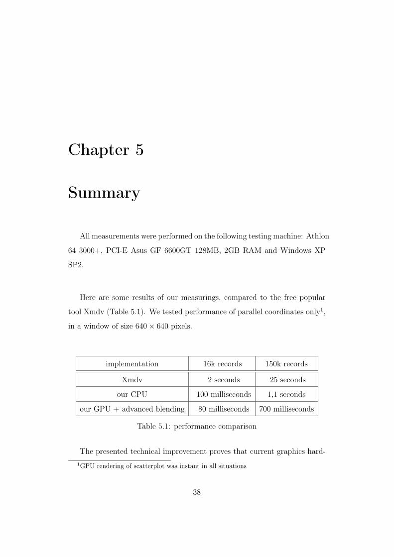
Here are some results of our measurings, compared to the free popular

tool Xmdv (Table 5.1). We tested performance of parallel coordinates only1,

in a window of size 640× 640 pixels.

implementation 16k records 150k records

Xmdv 2 seconds 25 seconds

our CPU 100 milliseconds 1,1 seconds

our GPU + advanced blending 80 milliseconds 700 milliseconds

Table 5.1: performance comparison

The presented technical improvement proves that current graphics hard-1GPU rendering of scatterplot was instant in all situations

38

ware can be used also for such a specific rendering task as the parallel coor-

dinates or scatterplot display. By exploiting features of the shader models

and parallel processing pipelines we achieved a significant performance boost.

The only bottleneck that the technical modifications can not improve is the

performance of the rasterization on the GPU.

As the wide variety of GPU functions and features grows with every

next generation of the graphics cards, there is much space for extending the

concept of hardware-accelerated information visualization. More and more

interaction tasks can be performed in parallel on the GPU, leaving the CPU

free for non-geometric or more data-oriented operations.

39

Bibliography

[1] E. R. TUFTE. Envisioning information. 1990.

[2] C. WARE. Information visualization: perception for design. 2000.

[3] STUART K. CARD, JOCK D. MACKINLAY, and BEN SHNEIDER-

MAN. Readings in information visualization: Using vision to think.

1999.

[4] R. KOSARA, H. HAUSER, and D. GRESH. An interaction view on

information visualization. EUROGRAPHICS 2003, 2003.

[5] S. EICK and G. WILLS. High interaction graphics. 1995.

[6] A. INSELBERG and B. DIMSDALE. Parallel coordinates: a tool for

visualizing multidimensional geometry. IEEE Visualization’90 Proceed-

ings, pages 361–378, 1990.

[7] JIMMY JOHANSSON PATRIC. Revealing structure within clustered

parallel coordinates displays, 2005.

[8] MANOJIT SARKAR and MARC H. BROWN. Graphical fisheye views

of graphs. 1992.

40

[9] PHILIPPE LACROUTE and MARC LEVOY. Fast volume rendering

using a shear-warp factorization of the viewing transformation. 1994,

Computer Graphics, 28(Annual Conference Series):451-458.

[10] ORION WILSON, ALLEN VANGELDER, and JANE WILHELMS. Di-

rect volume rendering via 3d textures. Technical Report UCSC-CRL-

94-19, June 29, 1994.

[11] M. Q. WANG BALDONADO, A. WOODRUFF, and A. KUCHINSKY.

Guidelines for using multiple views in information visualization. Pro-

ceedings of AVI 2000, Palermo, Italy, May 2000, pages 110–119, 2000.

[12] Xmdv. http://davis.wpi.edu/xmdv/.

[13] gDEBugger. http://www.gremedy.com/.

[14] JENS KRUGER. Linear algebra on gpus. SIGGRAPH 2005.

[15] nVidia SDK image histogram. http://developer.nvidia.com/page/tools.html.

41

Chapter 6

Abstrakt v Slovenčine

Dnešná technológia v pozadí vizualizácie má poskytnúť rýchle a presné

zobrazovanie a teda podporiť analýzu dát v prostredí vizualizácie informá-

cií1. Rozhodujúci element v procese skúmania dát je celková interaktívnosť,

špeciálne keď sa jedná o mnohorozmerné dáta. Avšak so stále rastúcim ob-

jemom dát, sa rýchle a interaktívne zobrazovanie ľahko stane statickým,

dávajúc iba pomalú až žiadnu interaktívnu spätnú väzbu.

Technické zlepšenia prezentované v tejto práci sú orientované na využi-

tie moderného hardvéru pre zmenu štandardného procesu zobrazovania po-

pulárnych techník v InfoVis, paralelných súradníc 2 a „scatterplot-u“, inter-

aktívnym spôsobom. Inteligentným využitím pokročilých vlastností, dnes už

bežne dostupného grafického hardvéru, sme dosiahli velké zlepšenie oproti

implementáciam, ktoré využívajú iba CPU, v rýchlosti zobrazovania a tiež

vo vizuálnej kvalite.

1InfoVis2parallel coordinates

42