UA

Aa

b

a

ARR1A

KLGPF

1

lgsopfstattc

U

h1

International Journal of Greenhouse Gas Control 46 (2016) 215–227

Contents lists available at ScienceDirect

International Journal of Greenhouse Gas Control

j ourna l h o mepage: www.elsev ier .com/ locate / i jggc

sing pulse testing for leakage detection in carbon storage reservoirs: field demonstration

lexander Y. Suna,∗, Jiemin Lua, Barry M. Freifeldb, Susan D. Hovorkaa, Akand Islama

Bureau of Economic Geology, Jackson School of Geosciences, University of Texas at Austin, Austin, TX, United StatesEarth Sciences Division, Lawrence Berkeley National Laboratory, Berkeley, CA, United States

r t i c l e i n f o

rticle history:eceived 31 July 2015eceived in revised form9 December 2015ccepted 12 January 2016

eywords:eakage detectioneological carbon sequestrationulse testingrequency domain analysis

a b s t r a c t

Monitoring techniques capable of deep subsurface detection are desirable for early warning and leakagepathway identification in geologic carbon storage formations. This work demonstrates the feasibility ofa pulse-testing-based leakage detection procedure, in which the storage reservoir is stimulated usingperiodic injection patterns and the acquired pressure perturbation signals are analyzed in the frequencydomain to detect potential deviations in the reservoir’s frequency domain responses. Unlike the tradi-tional well testing and associated time domain analyses, pulse testing aims to minimize the interferenceof reservoir operations and other ambient noise by selecting appropriate pulsing frequencies such thatreservoir responses to coded injection patterns can be uniquely determined in frequency domain. Fielddemonstration of this pulse-testing leakage detection technique was carried out at a CO2 enhanced oilrecovery site—the Cranfield site located in Mississippi, USA, which has long been used as a carbon storageresearch site. During the demonstration, two sets of pulsing experiments (baseline and leak tests) wereperformed using 90-min and 150-min pulsing periods to demonstrate feasibility of time-lapse leakage

Author's Copy

detection. For leak tests, an artificial leakage source was created through rate-controlled venting of CO2

from one of the monitoring wells because of the lack of known leakage pathways at the site. Our resultsshow that leakage events caused a significant deviation in the amplitude of the frequency response func-tion, indicating that pulse testing may be deployed as a cost-effective active monitoring technique, witha great potential for site-wide automated monitoring.

© 2016 Elsevier Ltd. All rights reserved.

. Introduction

Carbon capture and storage (CCS) is being pursued as aarge-scale mitigation option for making dramatic reductions inreenhouse gas emissions from power plants and other industrialources. A recent report by the International Energy Agency pointsut that CCS is the “only technology available today that has theotential to protect the climate while preserving the value of fossiluel reserves and existing infrastructure” (IEA, 2013). For geologictorage, supercritical CO2 is injected into deep geologic formationshat are typically located 1–3 km below surface (e.g., depleted oilnd gas reservoirs, unminable coal seams, or saline aquifers). Poten-

ial leakage through abandoned wells and geologic faults representhe greatest risk to geologic carbon storage projects. To ensureontainment efficiency and public safety, the fate and transport of

∗ Corresponding author at: University Station, Box X, Austin, TX 78713,nited States.

E-mail address: alex.sun@beg.utexas.edu (A.Y. Sun).

ttp://dx.doi.org/10.1016/j.ijggc.2016.01.015750-5836/© 2016 Elsevier Ltd. All rights reserved.

injected CO2 plume must be closely monitored during the life cycleof a geological sequestration project. Over the last decade, a widearray of monitoring methods have been developed and demon-strated for leakage detection, including pressure monitoring, soilgas monitoring, groundwater sampling, geophysical surveys, veg-etation stress, eddy covariance, and remote sensing (Lewicki et al.,2007; Trautz et al., 2012). Leakage pathways tend to be morediffused and the leak signals more attenuated as the distancefrom the source increases. Thus, monitoring methods/instrumentscapable of deep subsurface detection are more desirable for earlywarning and leakage pathway identification. Common methodssuitable for deep subsurface monitoring can be roughly classifiedinto surface-based and downhole technologies. The former mainlyincludes time-lapse seismic surveys, while the latter includes well-bore sensors and tools such as downhole pressure and temperaturegauges, fluid samplers, microseismic sensors, and distributed opti-

cal sensing cables.

Pressure sensing is one of the most studied and, arguably, mostwell established leakage detection methods for deep subsurfacemonitoring. A large number of analytical and numerical modeling

2 Green

wiae2Bodto2snCieelitca

cUslstrpnpuntspe

2

gl

Fl

's

16 A.Y. Sun et al. / International Journal of

orks have been performed to quantify pressure anomalies result-ng from focused leakage (e.g., from faults and abandoned wells)nd diffusive leakage (e.g., from leaky caprocks) (e.g., Nordbottent al., 2005; Cihan et al., 2011; Sun and Nicot, 2012; Sun et al.,013b; Kang et al., 2014; Dempsey et al., 2014; Heath et al., 2014;irkholzer et al., 2015). Major advantages of pressure sensing overther deep subsurface detection technologies include its (i) earlyetection potential; (ii) cost effectiveness; (iii) suitability for con-inuous, automated, long-term deployment; and (iv) suitability forptimal sensing or targeted monitoring (Jung et al., 2013; Sun et al.,013a; Jenkins et al., 2015; Hu et al., 2015). Concerns over pressureensing include its lack of sensitivity to “small” leaks and its prone-ess to noise interference, especially when deployed for monitoringO2 enhanced oil recovery (CO2-EOR) reservoirs. Notwithstand-

ng the large number of theoretical studies, relatively few fieldxperiments have been conducted to date to demonstrate theffectiveness and limitations associated with the pressure-basedeakage detection for carbon storage reservoirs. Here, a distinctions made between field experiments that are designed to quantifyhe effect of pressure responses to leakage and those that merelyollect pressure data as side products. We refer the former categorys active monitoring, while the latter as passive monitoring.

This paper presents results from a series of deep subsurface testsonducted recently at a CO2-EOR field near Cranfield, Mississippi,SA. These tests were exclusively designed to investigate the fea-

ibility of deploying pulse testing as a simple and cost-effectiveeakage detection technique. Pulse testing can be considered apecial type of pressure transient testing. During pulse testing,he injection rate is varied periodically while reservoir pressureesponses are continuously monitored in observation wells. Theressure data are then analyzed to characterize hydraulic commu-ication between wells and to infer reservoir parameters. Althoughulse testing has long been used in reservoir characterization, itsse for monitoring the integrity of carbon storage formations isew and, as far as we know, has never been tested in the field. Inhe following sections, we present the background of our field studyite, the experimental design and methodologies, field data inter-retation, and discussion. Finally, lessons learned from the fieldxperiment are summarized.

. Background of study site

Author

The Cranfield site has been used as a demonstration site foreologic carbon storage during the last seven years, under col-aboration between the Southeast Regional Carbon Sequestration

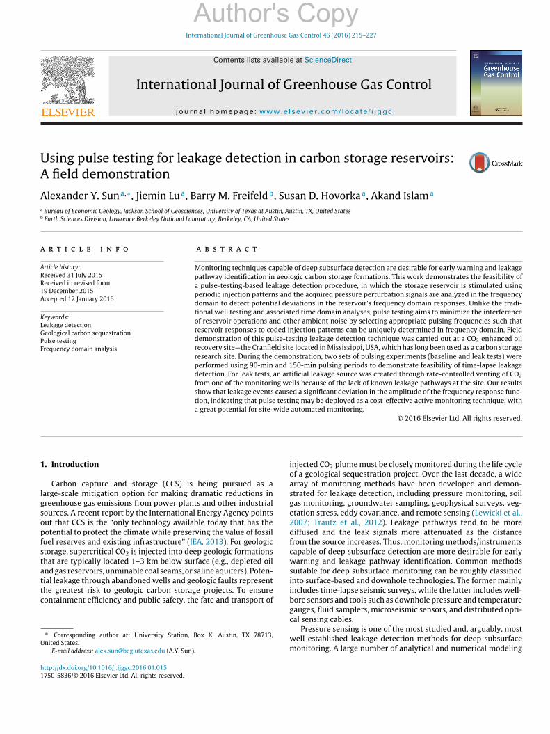
ig. 1. Areal view of the detailed area of study at Cranfield site (Lon: −91.141◦ , Lat: 31.56eak experiments, F3 was used as a “leaky” well. Locations of the flowback tank and traile

house Gas Control 46 (2016) 215–227

Partnership (SECARB) and Denbury Onshore LLC (Denbury). Oil andgas production originally started at the site in 1944. Gas recyclingwas used to maintain reservoir pressure until 1959, when the gascap was depleted. By 1966, most of the wells had been plugged andabandoned. The reservoir remained idle until Denbury began CO2flooding for EOR in July 2008. The source of CO2 was produced froma nearby natural source in Jackson Dome, Mississippi. The Cran-field site was originally selected by SECARB to develop the practiceof “stacked storage,” which would use the EOR operations to sup-port infrastructure setup, characterization, and public acceptancefor longer-term saline storage of CO2 (Hovorka et al., 2013).

The Cranfield reservoir is a four-way structural closure (with anorthwest-trending crestal graben) located about 3,010 m belowground surface. The reservoir formation comprises fluvial sand-stones and conglomerates of the Cretaceous lower TuscaloosaFormation, which is underlain by a regional unconformity on top ofshales and sandstones of the Dantzler Formation. The regional con-fining zone overlying the reservoir is 60 m of the middle Tuscaloosamarine mudstone. The CO2 injection interval at the Cranfield site islocally referred to as the D and E units, which range from 14 to 24 min thickness and were deposited as part of a laterally continuous butinternally complex fluvial formation comprised of fining-upwardsandstones and conglomerates. Chlorite coatings appear to havepreserved porosity and inhibited quartz cementation, but occludedpermeability. The stacking facies pattern of point-bar and channelsand bodies as found in the D–E units can have a significant impacton flow and transport paths, as many previous studies have shown(Knudby and Carrera, 2005; Sun et al., 2008). The reservoir tem-perature is about 129 ◦C, and reservoir pressure before CO2-EORstarted is around 32 MPa, which is close to the original hydrostaticpressure in place. The dip of the reservoir interval ranges from 1to 3 degrees. More detailed descriptions of the regional and sitegeology related to Cranfield can be found in Lu et al. (2012).

Many of the past research and development activities at theCranfield site had been conducted at its Detailed Area of Study(DAS) site, which consists of three colinear wells, including oneinjector (CFU31-F1) and two monitoring wells (CFU31-F2 andCFU31-F3) (Fig. 1). These three wells will be referred to as F1, F2, andF3 in the rest of this paper. The surface separation distance betweenF1 and F2 is 69.8 m, and between F2 and F3 it is 29.9 m. The bottom-hole distance between F1 and F2 is 60 m; between F1 and F3 it is

Copy

93 m; and between F2 and F3 it is 33.5 m. F2 and F3 were completedwith fiberglass casing to facilitate electrical resistance tomography(ERT) measurements and other well loggings during site character-ization. Fig. 2 shows the vertical distributions of permeability and

4◦), which consists of an injector (F1) and two monitoring wells (F2 and F3). Duringr area are also labeled.

A.Y. Sun et al. / International Journal of Greenhouse Gas Control 46 (2016) 215–227 217

0 20 40

3175

3180

3185

3190

3195

3200

3205

Dep

th (m

)

0 100 200

3175

3180

3185

3190

3195

3200

3205

Dep

th (m

)

0 20 40

3175

3180

3185

3190

3195

3200

3205

Dep

th (m

)

0 1000 2000

3175

3180

3185

3190

3195

3200

3205

Dep

th (m

)

CFU-F2 CFU-F3

(a) (b) (c) (d)

d from

ptfla

2udtdgdtnssmTspsS

tpa(pzo

Author's Copy

Porosity (%) Perm (md)

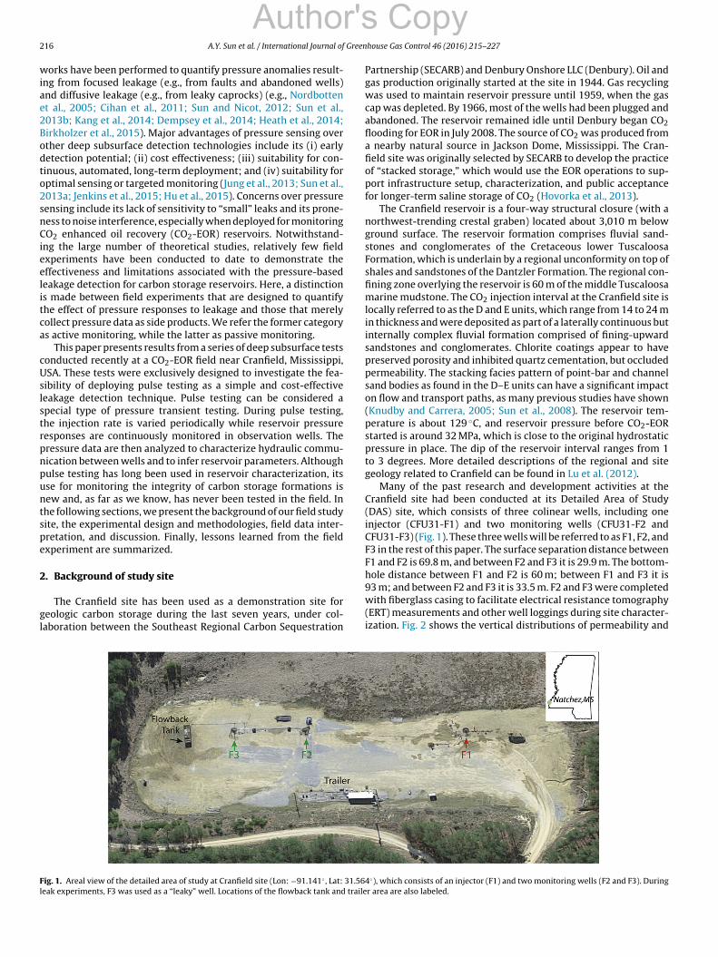
Fig. 2. Porosity and permeability profiles obtaine

orosity values obtained from core samples, which reflect the ver-ically and laterally heterogeneous nature of the lower Tuscaloosauvial formation. All three wells are located just outside the oil fieldnd completed in the water zone below the oil–water contact.

Injection of CO2 into brine at F1 was initiated on December 1,009 with an initial rate of 175 kg/min, which was increased grad-ally to 350 kg/min. Continuous fluid sampling was carried outuring the first month of CO2 injection, and two subsequent tracerests using sulfur hexafluoride and noble gases were conducted atifferent injection rates to measure flow velocity changes. A mainoal of that experiment was to obtain high-resolution monitoringata as the reservoir went through phase changes. Experimen-al results indicated that the DAS wells were connected throughumerous, separate fluid flow pathways (Lu et al., 2012). To confirmtorage permanence and track the CO2 plume pattern, crosswelleismic tomography was done before injection started and then 10onths after the initiation of injection (Ajo-Franklin et al., 2013).

he time-lapse seismic tomography revealed two spatial zones ofignificant CO2 saturation, which corresponds to zones of elevatedermeability in lower Tuscaloosa D and E units (Fig. 2) and are con-istent with results from time-lapse sonic logs and the Reservoiraturation Tool (RST) logs.

The injection rate at Cranfield has been about 1 million metricons per year since 2008 (Hovorka et al., 2013). High-resolutionressure gauges were initially deployed in both the reservoirnd the above-zone monitoring interval in a monitoring well

EGL-7) located near the center of the Cranfield site to monitorressure responses to the initiation of injection. The injectionone gauge showed a pressure increase within days of the startf injection and pressure increased steadily for 3 months, raising

Porosity (%) Perm (md)

core sample analyses for (a, b) F2 and (c, d) F3.

the reservoir pressure to approximately 5.2 MPa (754 psi) abovethe initial conditions (Meckel et al., 2008). Experience gained fromEGL-7 suggests that continuous pressure monitoring has merits incapturing high-frequency pressure variations. However, isolatingthe causes of these variations was challenging using passivemonitoring alone because of the ambiguity caused by reservoiroperations (Hovorka et al., 2013). In contrast, the time-lapse pulse-testing leakage detection proposed in this study is an appealing,active monitoring technique that is designed to counteract noiseinterference to pressure signals. In the next section, we describethe main principles underlying pulse testing and provide detailson field experimental design and execution.

3. Methodology

3.1. Pulse testing

Pulse testing was originally introduced to reservoir characteri-zation in the 1960s (Johnson et al., 1966). Since then, the technologyhas been demonstrated for crosswell pressure transient testing inmany reservoir studies (e.g., McKinley et al., 1968; Beliveau, 1989;Fokker and Verga, 2011). The simplest pulse testing involves theuse of square or rectangular pulses. If conditions permit, harmonicpulse testing (HPT) may also be done, in which case sinusoidal exci-tation to the reservoir is introduced through the pulser well andpressure responses are continuously monitored in both the pulser

well and the monitoring well(s). Compared to square pulses, HPTdata are easier to analyze because only a single sinusoid is involvedper test; however, the test itself is more complicated to adminis-ter and requires special equipment to generate sinusoidal rates. So

2 Green

frSC22

veaoMer(

thTb

P

wωpaiAtsftV

tt

P

wrraqcaita�v1piforc

pdta

's

18 A.Y. Sun et al. / International Journal of

ar, HPT has been investigated mainly in analytical and numericaleservoir modeling (Hollaender et al., 2002; Ahn and Horne, 2010;un et al., 2015), groundwater applications (Rasmussen et al., 2003;ardiff et al., 2013; Guiltinan and Becker, 2015; Renner and Messar,006), and laboratory core sample characterization (Bernabé et al.,006).

By design, the interference of instrumentation noise and reser-oir operations can be significantly suppressed or even completelyliminated in pulse testing by selecting a priori the pulsing periodsnd, thereby, frequencies of signals. Such is the main advantagef active pressure monitoring over passive pressure monitoring.oreover, repeating pulse testing at multiple pulsing periods may

xtract additional information on reservoir properties and improveeservoir parameter estimation, as shown in previous studiesCardiff et al., 2013; Fokker and Verga, 2011).

Using Fourier expansion, the pulse function applied at an injec-or can be approximated using superposition of sinusoids, eachaving a frequency that is a multiple of the fundamental frequency.he corresponding pressure response at a monitoring well can thene approximated as

(r, t) =N∑

n=1

An sin(nωt + �n), (1)

here P is pressure, r is distance from the pulser, t is elapsed time, = 2�/T is the fundamental frequency determined by the pulsingeriod T, and An and �n represent the amplitude and phase associ-ted with the nth sinusoid, respectively. It can be shown throughntegration that the square pulse contains only odd multiples of ω.ccording to the Nyquist sampling theorem, the highest frequency

hat can be resolved is determined by 1/(2�t), where �t is theampling interval. Eq. (1) implies that pressure responses acquiredrom pulse testing can be analyzed using similar frequency-domainechniques developed for HPT (Ahn and Horne, 2010; Fokker anderga, 2011; Sun et al., 2015).

Let Pinj and Pobj denote the pressure responses obtained fromhe injector and a monitoring well, the excitation–response rela-ionship of the reservoir is given by the convolution integral

obs =∫ t

0

Pinj(t − �)g(�)d�, (2)

here g(·) is the transfer or kernel function. Let Pinj and Pobs rep-esent the Fourier transform of Pinj and Pobj, the system frequencyesponse function H(ω) (i.e., the Fourier transform of g(·)) is defineds the ratio between Pobs and Pinj , namely, H(ω) = Pobs/Pinj . The fre-uency response function depends on mobility, porosity, and totalompressibility of the reservoir under study, and thus it provides

characterization of the reservoir’s excitation-response behaviorn frequency domain. For homogeneous isotropic reservoirs, pulseesting determines the value of mobility-thickness product (kb/�)nd porosity-compressibility-thickness product (�ctb), where k, b,, �, and ct represent permeability, effective reservoir thickness,iscosity, porosity, and total compressibility, respectively (Kamal,983). In this work, the frequency-domain data are used to estimatearameters through an analytical forward model. Each data point

n frequency domain represents system responses to a particularrequency embedded in the pulsing signal (see Eq. (1)). By focusingnly on those frequencies with meaningful data, the ambiguitieselated to time domain analyses, especially those caused by noise,an be lessened.

The main idea behind pulse-testing-based leakage detection

Author

rocedure is that if one or more new leaks occur within theetectable range of an observer, the observer’s pressure responseso pulser will be modified, which then leads to an observable devi-tion in H(ω) from its baseline. Thus, this technique is similar to

house Gas Control 46 (2016) 215–227

time-lapse seismic methods in principle. When deployed as a rou-tine monitoring method, each pulse test without anomaly can inturn serve as the baseline for the next test. The requirement of abaseline is common among time-lapse monitoring methods. Alter-natively, a forward model can be developed to predict the nominalsystem behavior (i.e., in absence of leakage) in lieu of the baseline.The latter aspect is examined in the following analyses in Section4.3.

In a multiphase fluid setting, it is commonly assumed that theinjected fluid displaces the ambient fluid in a piston-like fashionsuch that two fluid banks are formed and the saturation gradi-ent within each fluid zone is approximately zero (Abbaszadeh andKamal, 1989). Theoretical and numerical validation of the time-lapse HPT leakage detection concept have been provided in Sunet al. (2014, 2015) for single- and multiphase flows. In general, theamplitude of H(ω) decreases monotonically with increasing pulsefrequency. Longer pulsing periods may help probe leaks locatedfarther away (provided that the observation well is still sensitiveto both the pulser and leaks), but at the expense of longer exper-iment time. For carbon storage reservoirs, the authors suggestedthat the fluid condition at observation locations should not changesignificantly between two HPTs for the time-lapse method to givemeaningful results.

The purpose of our Cranfield DAS experiment is to provide afield-scale validation of the pulse-testing leakage detection con-cept. CO2 flooding at the injector F1 has been ongoing sinceDecember 2009. At Cranfield site, the operator injects CO2 contin-uously rather than using the conventional water-alternating gasEOR strategy. For those reasons, it was expected that the injectioninterval underneath the DAS site is mostly saturated with super-critical CO2 and the nonlinear effect related to multiphase flows isminimal. Also, fluid conditions between different sets of pulse testswere not expected to change significantly.

3.2. Field experiment design and procedure

The field campaign consists of baseline and leak experiments,which were conducted sequentially. Before the field experiments,high-resolution permanent downhole gauges (Ranger PermanentHybrid Digital Addressable Surface Read Out Gauge, Ranger GaugeSystems, Sugar Land, Texas, USA) were installed in well F2 andF3 on December 16–17, 2014. The control lines in each well con-sist of hybrid fiber-optic electrical cables encapsulated in 0.635-cm(1/4-in.) stainless steel tubing and were installed using a capillaryinjection unit through a lubricator and packoff. Resolution of thepressure gauge is 68.9 Pa (0.01 psi) and its data polling frequency isset to every 2 s. As discussed below, these highly sensitive pressuregauges are necessary to detect small pressure anomalies. Recordskept by our well management subcontractor (Sandia Technologies,LLC, Houston, TX, USA) show that the depth of the downhole gaugeassembly is 3221.1 m (10,568 ft) in F2 and 3222.0 m (10,571 ft)in F3. Ideally, the bottom-hole pressure (BHP) at F1 should alsobe monitored during the experiment to normalize the frequencyresponse function, H(ω). However, it was not an option for thisproject. Thus, we mainly used the monitoring well data duringanalyses.

For the baseline, two sets of pulse testing experiments were per-formed on January 19 and January 20, 2015, one using a 90-minperiod and the other using a 150-min period. Each period startswith a shutin half cycle (50% of the time), followed by a constant-rate injection half cycle. These pulses were introduced to F1 bymanually turning on/off the wellhead choke valve. F2 was used as

Copy

the monitoring well in all experiments.The actual pulse testing does not require additional equipment

other than pressure gauges. However, because there is no knownleakage pathway at the DAS site, for demonstration F3 was used to

A.Y. Sun et al. / International Journal of Greenhouse Gas Control 46 (2016) 215–227 219

F3 WellheadWing Valve

Micromotion Flowmeter

To Gas Buster

ReducingBushing 1” x ½”

T2

P2

T1

P1

Equipment @ F3

Norman Filter

Fluid Sampling Port

ReducingBushing

2” x ½”

dP1

T Temperature

P Pressure

F into

m ollect

cpbwfFiiCatflPoutmrt

p“Jgsalarb

ciwiwwcpti

Author's Copy

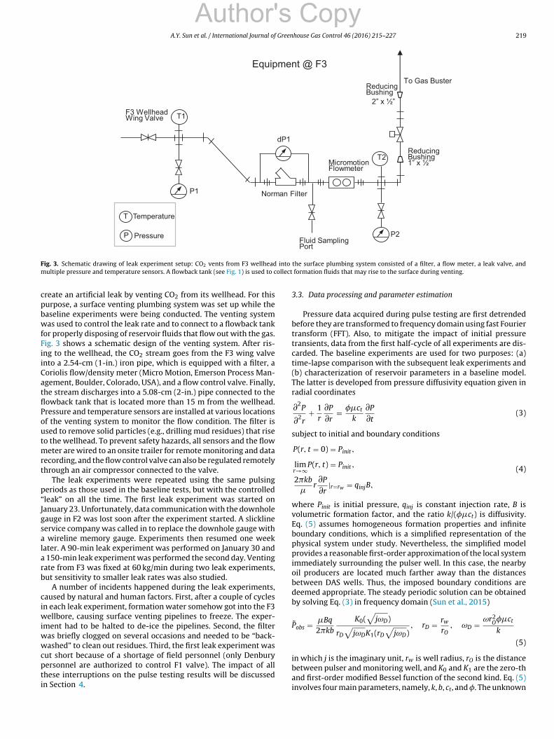
ig. 3. Schematic drawing of leak experiment setup: CO2 vents from F3 wellheadultiple pressure and temperature sensors. A flowback tank (see Fig. 1) is used to c

reate an artificial leak by venting CO2 from its wellhead. For thisurpose, a surface venting plumbing system was set up while theaseline experiments were being conducted. The venting systemas used to control the leak rate and to connect to a flowback tank

or properly disposing of reservoir fluids that flow out with the gas.ig. 3 shows a schematic design of the venting system. After ris-ng to the wellhead, the CO2 stream goes from the F3 wing valvento a 2.54-cm (1-in.) iron pipe, which is equipped with a filter, aoriolis flow/density meter (Micro Motion, Emerson Process Man-gement, Boulder, Colorado, USA), and a flow control valve. Finally,he stream discharges into a 5.08-cm (2-in.) pipe connected to theowback tank that is located more than 15 m from the wellhead.ressure and temperature sensors are installed at various locationsf the venting system to monitor the flow condition. The filter issed to remove solid particles (e.g., drilling mud residues) that riseo the wellhead. To prevent safety hazards, all sensors and the flow

eter are wired to an onsite trailer for remote monitoring and dataecording, and the flow control valve can also be regulated remotelyhrough an air compressor connected to the valve.

The leak experiments were repeated using the same pulsingeriods as those used in the baseline tests, but with the controlledleak” on all the time. The first leak experiment was started onanuary 23. Unfortunately, data communication with the downholeauge in F2 was lost soon after the experiment started. A slicklineervice company was called in to replace the downhole gauge with

wireline memory gauge. Experiments then resumed one weekater. A 90-min leak experiment was performed on January 30 and

150-min leak experiment was performed the second day. Ventingate from F3 was fixed at 60 kg/min during two leak experiments,ut sensitivity to smaller leak rates was also studied.

A number of incidents happened during the leak experiments,aused by natural and human factors. First, after a couple of cyclesn each leak experiment, formation water somehow got into the F3

ellbore, causing surface venting pipelines to freeze. The exper-ment had to be halted to de-ice the pipelines. Second, the filter

as briefly clogged on several occasions and needed to be “back-ashed” to clean out residues. Third, the first leak experiment was

ut short because of a shortage of field personnel (only Denburyersonnel are authorized to control F1 valve). The impact of allhese interruptions on the pulse testing results will be discussedn Section 4.

the surface plumbing system consisted of a filter, a flow meter, a leak valve, and formation fluids that may rise to the surface during venting.

3.3. Data processing and parameter estimation

Pressure data acquired during pulse testing are first detrendedbefore they are transformed to frequency domain using fast Fouriertransform (FFT). Also, to mitigate the impact of initial pressuretransients, data from the first half-cycle of all experiments are dis-carded. The baseline experiments are used for two purposes: (a)time-lapse comparison with the subsequent leak experiments and(b) characterization of reservoir parameters in a baseline model.The latter is developed from pressure diffusivity equation given inradial coordinates

∂2P

∂2r

+ 1r

∂P

∂r= ��ct

k

∂P

∂t(3)

subject to initial and boundary conditions

P(r, t = 0) = Pinit,

limr→∞

P(r, t) = Pinit,

2�kb

�r∂P

∂r|r=rw = qinjB,

(4)

where Pinit is initial pressure, qinj is constant injection rate, B isvolumetric formation factor, and the ratio k/(��ct) is diffusivity.Eq. (5) assumes homogeneous formation properties and infiniteboundary conditions, which is a simplified representation of thephysical system under study. Nevertheless, the simplified modelprovides a reasonable first-order approximation of the local systemimmediately surrounding the pulser well. In this case, the nearbyoil producers are located much farther away than the distancesbetween DAS wells. Thus, the imposed boundary conditions aredeemed appropriate. The steady periodic solution can be obtainedby solving Eq. (3) in frequency domain (Sun et al., 2015)

Pobs = �Bq

2�kb

K0(√

jωD)

rD

√jωDK1(rD

√jωD)

, rD = rw

rO, ωD = ωr2

O��ct

k

(5)

in which j is the imaginary unit, rw is well radius, rO is the distancebetween pulser and monitoring well, and K0 and K1 are the zero-thand first-order modified Bessel function of the second kind. Eq. (5)involves four main parameters, namely, k, b, ct, and �. The unknown

220 A.Y. Sun et al. / International Journal of Greenhouse Gas Control 46 (2016) 215–227

12:00 13:00 14:00 15:00 16:00 17:00 18:004717.5

4718

4718.5

Time

Pre

ssur

e (p

si)

(a) 90−min baseline @F2, raw data

1810

3620

Pul

se@

F1(b

bl/d

ay)

12:00 13:00 14:00 15:00 16:00 17:00 18:00−0.5

−0.25

0

0.25

0.5

Time

ΔP

(psi

)

(b) ΔP @F2, after trend removal

12:00 13:00 14:00 15:00 16:00 17:00 18:004715.8

4716

4716.2

4716.4

4716.6

Time

Pre

ssur

e (p

si)

(c) 90−min baseline @F3, raw data

1810

3620

Pul

se@

F1(b

bl/d

ay)

12:00 13:00 14:00 15:00 16:00 17:00 18:00−0. 5

−0.25

0

0.25

0.5

Time

ΔP

(psi

)

(d) ΔP @F3, after trend removal

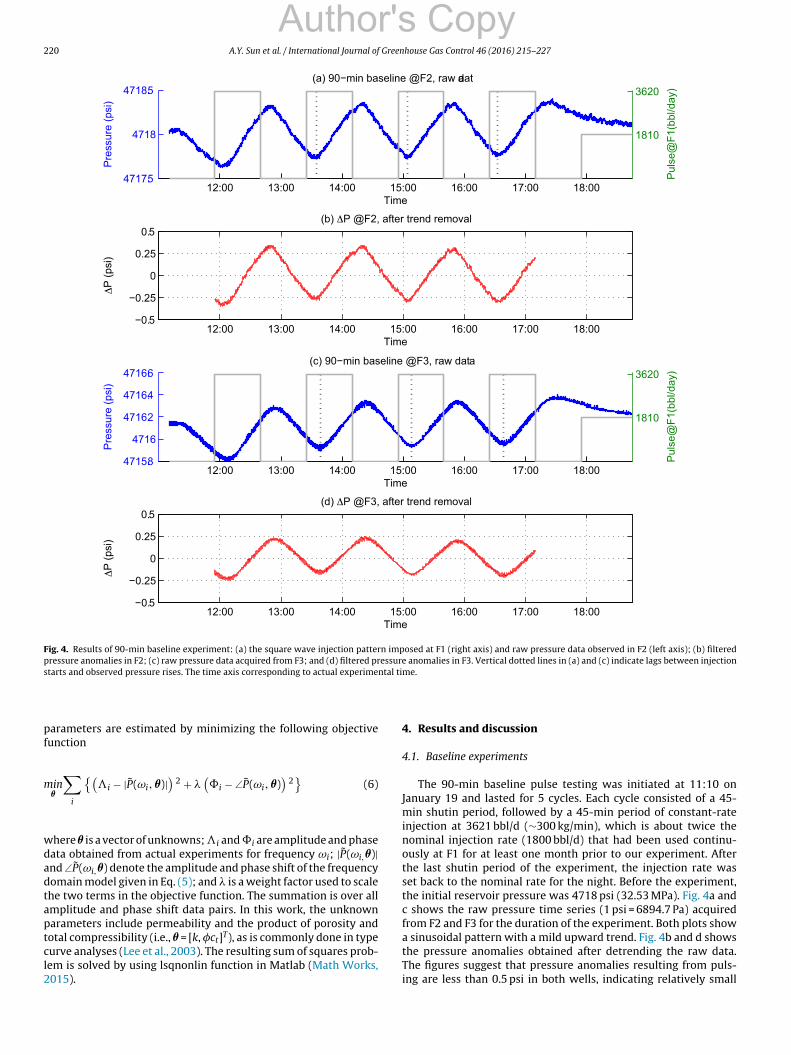
Fig. 4. Results of 90-min baseline experiment: (a) the square wave injection pattern imposed at F1 (right axis) and raw pressure data observed in F2 (left axis); (b) filteredpressure anomalies in F2; (c) raw pressure data acquired from F3; and (d) filtered pressure anomalies in F3. Vertical dotted lines in (a) and (c) indicate lags between injections ntal ti

pf

m

wdadtaptcl2

Author's Copy

tarts and observed pressure rises. The time axis corresponding to actual experime

arameters are estimated by minimizing the following objectiveunction

in�

∑i

{(i − |P(ωi, �)|

)2 +

(�i − ∠P(ωi, �)

)2}

(6)

here � is a vector of unknowns; i and �i are amplitude and phaseata obtained from actual experiments for frequency ωi; |P(ωi,�)|nd ∠P(ωi,�) denote the amplitude and phase shift of the frequencyomain model given in Eq. (5); and is a weight factor used to scalehe two terms in the objective function. The summation is over allmplitude and phase shift data pairs. In this work, the unknownarameters include permeability and the product of porosity and

otal compressibility (i.e., � = [k, �ct]T), as is commonly done in typeurve analyses (Lee et al., 2003). The resulting sum of squares prob-em is solved by using lsqnonlin function in Matlab (Math Works,015).

me.

4. Results and discussion

4.1. Baseline experiments

The 90-min baseline pulse testing was initiated at 11:10 onJanuary 19 and lasted for 5 cycles. Each cycle consisted of a 45-min shutin period, followed by a 45-min period of constant-rateinjection at 3621 bbl/d (∼300 kg/min), which is about twice thenominal injection rate (1800 bbl/d) that had been used continu-ously at F1 for at least one month prior to our experiment. Afterthe last shutin period of the experiment, the injection rate wasset back to the nominal rate for the night. Before the experiment,the initial reservoir pressure was 4718 psi (32.53 MPa). Fig. 4a andc shows the raw pressure time series (1 psi = 6894.7 Pa) acquiredfrom F2 and F3 for the duration of the experiment. Both plots show

a sinusoidal pattern with a mild upward trend. Fig. 4b and d showsthe pressure anomalies obtained after detrending the raw data.The figures suggest that pressure anomalies resulting from puls-ing are less than 0.5 psi in both wells, indicating relatively small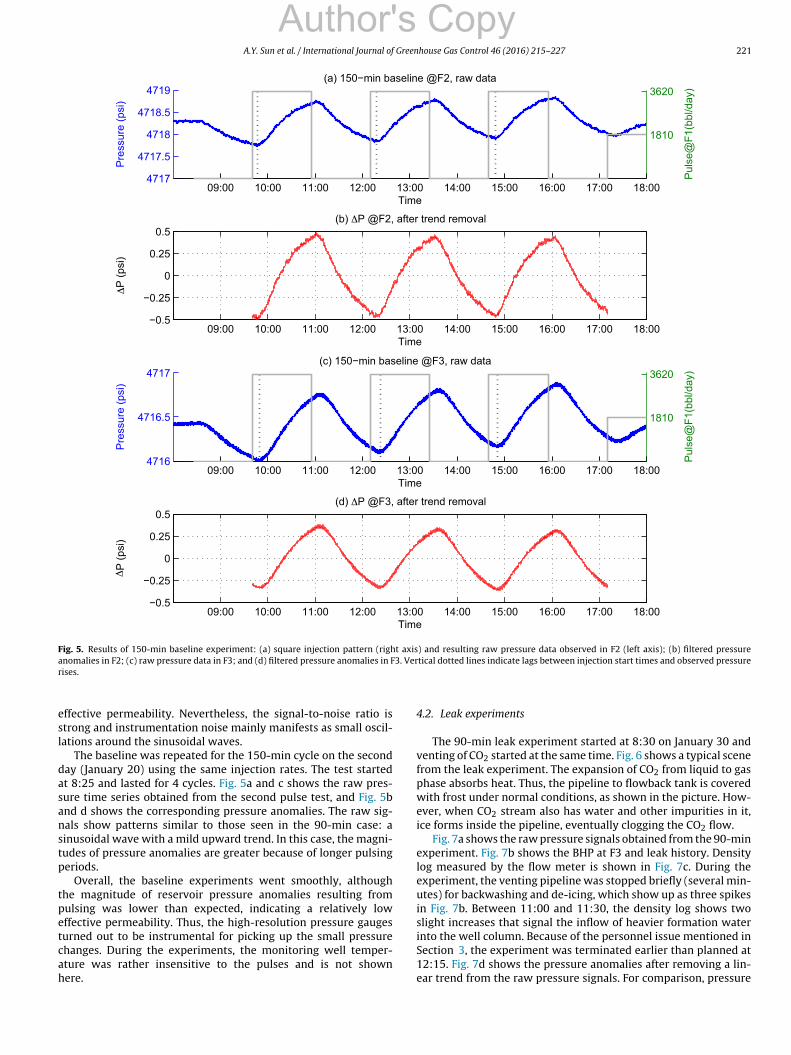

A.Y. Sun et al. / International Journal of Greenhouse Gas Control 46 (2016) 215–227 221

09:00 10:00 11:00 12:00 13:00 14:00 15:00 16:00 17:00 18:004717

4717.5

4718

4718.5

4719

Time

Pre

ssur

e (p

si)

(a) 150−min baseline @F2, raw data

1810

3620

Pul

se@

F1(b

bl/d

ay)

09:00 10:00 11:00 12:00 13:00 14:00 15:00 16:00 17:00 18:00−0.5

−0.25

0

0.25

0.5

Time

ΔP

(psi

)

(b) ΔP @F2, after trend removal

09:00 10:00 11:00 12:00 13:00 14:00 15:00 16:00 17:00 18:004716

4716.5

4717

Time

Pre

ssur

e (p

si)

(c) 150−min baseline @F3, raw data

1810

3620

Pul

se@

F1(b

bl/d

ay)

09:00 10:00 11:00 12:00 13:00 14:00 15:00 16:00 17:00 18:00−0. 5

−0.25

0

0.25

0.5

Time

ΔP

(psi

)

(d) ΔP @F3, after trend removal

Fig. 5. Results of 150-min baseline experiment: (a) square injection pattern (right axis) and resulting raw pressure data observed in F2 (left axis); (b) filtered pressurea 3. Verr

esl

dasanstp

tpetcah

Author's Copy

nomalies in F2; (c) raw pressure data in F3; and (d) filtered pressure anomalies in Fises.

ffective permeability. Nevertheless, the signal-to-noise ratio istrong and instrumentation noise mainly manifests as small oscil-ations around the sinusoidal waves.

The baseline was repeated for the 150-min cycle on the seconday (January 20) using the same injection rates. The test startedt 8:25 and lasted for 4 cycles. Fig. 5a and c shows the raw pres-ure time series obtained from the second pulse test, and Fig. 5bnd d shows the corresponding pressure anomalies. The raw sig-als show patterns similar to those seen in the 90-min case: ainusoidal wave with a mild upward trend. In this case, the magni-udes of pressure anomalies are greater because of longer pulsingeriods.

Overall, the baseline experiments went smoothly, althoughhe magnitude of reservoir pressure anomalies resulting fromulsing was lower than expected, indicating a relatively lowffective permeability. Thus, the high-resolution pressure gauges

urned out to be instrumental for picking up the small pressurehanges. During the experiments, the monitoring well temper-ture was rather insensitive to the pulses and is not shownere.

tical dotted lines indicate lags between injection start times and observed pressure

4.2. Leak experiments

The 90-min leak experiment started at 8:30 on January 30 andventing of CO2 started at the same time. Fig. 6 shows a typical scenefrom the leak experiment. The expansion of CO2 from liquid to gasphase absorbs heat. Thus, the pipeline to flowback tank is coveredwith frost under normal conditions, as shown in the picture. How-ever, when CO2 stream also has water and other impurities in it,ice forms inside the pipeline, eventually clogging the CO2 flow.

Fig. 7a shows the raw pressure signals obtained from the 90-minexperiment. Fig. 7b shows the BHP at F3 and leak history. Densitylog measured by the flow meter is shown in Fig. 7c. During theexperiment, the venting pipeline was stopped briefly (several min-utes) for backwashing and de-icing, which show up as three spikesin Fig. 7b. Between 11:00 and 11:30, the density log shows twoslight increases that signal the inflow of heavier formation water

into the well column. Because of the personnel issue mentioned inSection 3, the experiment was terminated earlier than planned at12:15. Fig. 7d shows the pressure anomalies after removing a lin-ear trend from the raw pressure signals. For comparison, pressure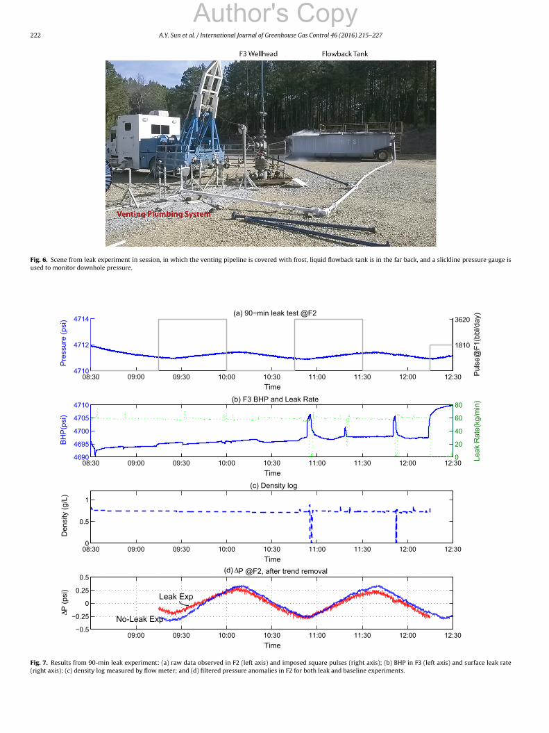

222 A.Y. Sun et al. / International Journal of Greenhouse Gas Control 46 (2016) 215–227

Fig. 6. Scene from leak experiment in session, in which the venting pipeline is covered with frost, liquid flowback tank is in the far back, and a slickline pressure gauge isused to monitor downhole pressure.

09:00 12:004710

4712

4714

Time

Pre

ssur

e (p

si)

(a) 90−min leak test @F2

1810

3620

Pul

se@

F1(b

bl/d

ay)

08:30 09:00 09:30 10:00 10:30 11:00 11:30 12:00 12:304690

4695

4700

4705

4710

Time

BH

P(p

si)

(b) F3 BHP and Leak Rate

0

20

40

60

80

Leak

Rat

e(kg

/min

)

08:30 09:00 09:30 10:00 10:30 11:00 11:30 12:00 12:300

0.5

1

Time

Den

sity

(g/L

)

(c) Density log

09:00 09:30 10:00 10:30 11:00 11:30 12:00 12:30−0.5

−0.25

0

0.25

0.5

Time

Δ P (p

si)

(d) ΔP @F2, after trend removal

08:30 09:30 10:00 10:30 11:00 11:30 12:30

Leak Exp

No-Leak Exp

Fig. 7. Results from 90-min leak experiment: (a) raw data observed in F2 (left axis) and imposed square pulses (right axis); (b) BHP in F3 (left axis) and surface leak rate(right axis); (c) density log measured by flow meter; and (d) filtered pressure anomalies in F2 for both leak and baseline experiments.

Author's Copy

A.Y. Sun et al. / International Journal of Greenhouse Gas Control 46 (2016) 215–227 223

09:00 12:00 15:00Time

Pre

ssur

e (p

si)

(a) 150−min leak test @F2

1810

3620

Pul

se@

F1(b

bl/d

ay)

09:00 10:00 11:00 12:00 13:00 14:00 15:004690

4700

4710

4720

Time

BH

P(p

si)

(b) F3 BHP and Leak Rate

0

50

100

150

Leak

Rat

e(kg

/min

)

09:00 10:00 11:00 12:00 13:00 14:00 15:000

0.5

1

Time

Den

sity

(g/L

)

(c) Density log

09:00 10:00 11:00 12:00 13:00 14:00 15:00−0.5

−0.25

0

0.25

0.5

Time

ΔP

(psi

)

(d) ΔP @F2, after trend removal

10:00 11:00 13:00 14:00

F ) and

(

ainst

VfciargmFiw

ftscr

Author's Copy

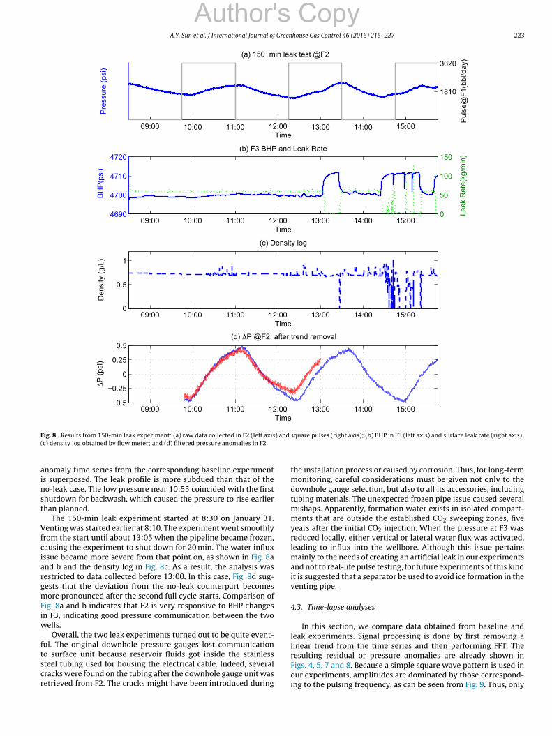
ig. 8. Results from 150-min leak experiment: (a) raw data collected in F2 (left axisc) density log obtained by flow meter; and (d) filtered pressure anomalies in F2.

nomaly time series from the corresponding baseline experiments superposed. The leak profile is more subdued than that of theo-leak case. The low pressure near 10:55 coincided with the firsthutdown for backwash, which caused the pressure to rise earlierhan planned.

The 150-min leak experiment started at 8:30 on January 31.enting was started earlier at 8:10. The experiment went smoothly

rom the start until about 13:05 when the pipeline became frozen,ausing the experiment to shut down for 20 min. The water influxssue became more severe from that point on, as shown in Fig. 8and b and the density log in Fig. 8c. As a result, the analysis wasestricted to data collected before 13:00. In this case, Fig. 8d sug-ests that the deviation from the no-leak counterpart becomesore pronounced after the second full cycle starts. Comparison of

ig. 8a and b indicates that F2 is very responsive to BHP changesn F3, indicating good pressure communication between the two

ells.Overall, the two leak experiments turned out to be quite event-

ul. The original downhole pressure gauges lost communication

o surface unit because reservoir fluids got inside the stainlessteel tubing used for housing the electrical cable. Indeed, severalracks were found on the tubing after the downhole gauge unit wasetrieved from F2. The cracks might have been introduced during

square pulses (right axis); (b) BHP in F3 (left axis) and surface leak rate (right axis);

the installation process or caused by corrosion. Thus, for long-termmonitoring, careful considerations must be given not only to thedownhole gauge selection, but also to all its accessories, includingtubing materials. The unexpected frozen pipe issue caused severalmishaps. Apparently, formation water exists in isolated compart-ments that are outside the established CO2 sweeping zones, fiveyears after the initial CO2 injection. When the pressure at F3 wasreduced locally, either vertical or lateral water flux was activated,leading to influx into the wellbore. Although this issue pertainsmainly to the needs of creating an artificial leak in our experimentsand not to real-life pulse testing, for future experiments of this kindit is suggested that a separator be used to avoid ice formation in theventing pipe.

4.3. Time-lapse analyses

In this section, we compare data obtained from baseline andleak experiments. Signal processing is done by first removing alinear trend from the time series and then performing FFT. The

resulting residual or pressure anomalies are already shown inFigs. 4, 5, 7 and 8. Because a simple square wave pattern is used inour experiments, amplitudes are dominated by those correspond-ing to the pulsing frequency, as can be seen from Fig. 9. Thus, only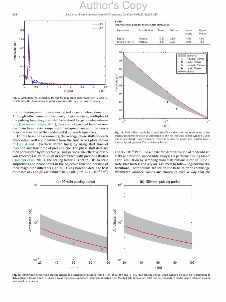

224 A.Y. Sun et al. / International Journal of Greenhouse Gas Control 46 (2016) 215–227

0 0.5 1 1.5 2 2.5 3 3.5

x 10−3

0

0.05

0.1

0.15

0.2

0.25

0.3

ω (1/s)

Am

plitu

de (p

si)

F2F3

Fw

tAttor

oiitv(ate

Table 1Prior statistics used for Monte Carlo simulation.

Parameter Distribution Mean Std. dev. Lowerbound

Upperbound

log(k) Normal 0.37 0.55 −4.61 4.61log [(�ct)1010] Normal −2.43 0.25 −6.91 1.61

10−5 10−4 10 −30.1

0.2

0.3

0.4

0.5

0.6

0.7

0.8

0.9

ω (s−1)

Am

plitu

de (p

si)

Model CINoLeak, 90minLeak, 90mi nNoLeak, 150mi nLeak, 90minModel

Fig. 11. Leak (filled symbols) caused significant deviation in amplitudes of fre-

Carlo simulation by sampling from distributions listed in Table 1.

Fde

Author's Copy

ig. 9. Amplitude vs. frequency for the 90-min pulse experiment for F2 and F3,hich show the dominating amplitudes occur at the base pulsing frequency.

he dominating amplitudes are extracted for parameter estimation.lthough other non-zero frequency responses (e.g., multiples of

he pulsing frequency) can also be utilized for parameter estima-ion (Fokker and Verga, 2011), they are not pursued here becauseur main focus is on comparing time-lapse changes in frequencyesponse function at the fundamental pulsing frequencies.

For the baseline experiments, the average phase shifts for eachbservation well are identified from the time series plots shownn Figs. 4 and 5 (vertical dotted lines) by using start time ofnjection and start time of pressure rise. The phase shift data arehen normalized by respective pulsing periods. The effective reser-oir thickness is set to 25 m in accordance with previous studiesHosseini et al., 2013). The scaling factor is set to 0.01 to scale

mplitudes and phase shifts in the objective function because ofheir magnitude differences, Eq. (6). Using baseline data, the beststimates of k and �ct are found to be 1.5 mD (1 mD = 1 × 10−15 m2)

20 40 60 80 10010−1

100

101(a) 90−min pulsing period

r (m)

Am

plitu

de (p

si)

ig. 10. Amplitude of observed pulsing signals as a function of distance from F1 for (a) 9ata obtained from F2 and F3. Shaded areas represent confidence intervals estimated frostimated parameters.

quency response function as compared to the no-leak case (open symbols). Solidline is calculated using estimated reservoir parameter values and shaded area isformed by using lower 95% confidence bound.

and 9 × 10−12 Pa−1. To facilitate the demonstration of model-basedleakage detection, uncertainty analyses is performed using Monte

Note that both k and �ct are assumed to follow log-normal dis-tributions. Their bounds are set on the basis of prior knowledge.Parameter variance values are chosen in such a way that the

20 40 60 80 10010−1

100

101(b) 150−min pulsing period

r (m)

Am

plitu

de (p

si)

0-min and (b) 150-min pulsing period. Open symbols on each plot correspond tom Monte Carlo simulation, solid line corresponds to model values calculated using

Green

abtb

upottmohsp(afiDuH

Fr

s

A.Y. Sun et al. / International Journal of

mplitude deviations are just outside the confidence bounds of theaseline model (see discussion below). A large number of realiza-ions (20,000) are used in lieu of more delicate sampling schemesecause the analytical model is fast to run.

The estimated effective permeability is relatively low but notnreasonable. Previously, Ajo-Franklin et al. (2013) estimated theermeability and porosity values to be 64 mD and 0.25 on the basisf F2 core samples. It is well known that crosswell testing reflectshe effective formation properties of the reservoir volume betweenhe pulser and observation well pair, whereas core sample analysis

ainly provides point property estimates and may not be extrap-lated to large distances beyond the logged well, especially foreterogeneous formations. On the basis of their U-tube samplingtudies, Lu et al. (2012) noted that at the DAS site multiple flowathways exist over a distance of tens of meters. Hosseini et al.2013) could not identify a good linear correlation between porositynd log permeability using core sample data from six wells at Cran-eld site. Thus, because of the highly complex nature of the fluvial

Author'

–E units, it is not surprising that effective permeability estimatedsing pulse testing data differs from the core sample estimates.owever, a key difference between our experiments and the 2009

16:00 16:15 16:30 16:45 17:00 17:1−0.1

−0.05

0

0.05

0.1

0.15

Tim

ΔP

@F2

(p

si)

(a) Δ P @

16:00 16:15 16:30 16:45 17:00 17:14709

4710

4711

4712

Tim

BH

P (p

si)

(b) F3 BHP and

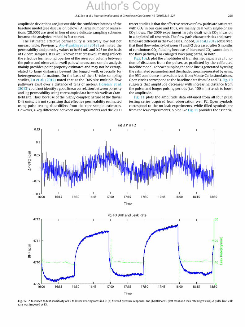
ig. 12. A test used to test sensitivity of F2 to lower venting rates in F3: (a) filtered pressuate was imposed at F3.

house Gas Control 46 (2016) 215–227 225

tracer studies is that the effective reservoir flow paths are saturatedwith CO2 in our case and thus, we mainly deal with single-phaseCO2 flows. The 2009 experiment largely dealt with CO2 invasionin a depleted oil reservoir. The flow path characteristics and traveltimes are different in the two cases. Indeed, Lu et al. (2012) observedthat fluid flow velocity between F1 and F2 decreased after 5 monthsof continuous CO2 flooding because of increased CO2 saturation inthe flow pathways or enlarged sweeping paths, or both.

Figs. 10a,b plot the amplitudes of transformed signals as a func-tion of distances from the pulser, as predicted by the calibratedbaseline model. For each subplot, the solid line is generated by usingthe estimated parameters and the shaded area is generated by usingthe 95% confidence interval derived from Monte Carlo simulations.Open circles correspond to the baseline data from F2 and F3. Fig. 10suggests that amplitude decreases with increasing distance fromthe pulser and longer pulsing periods (i.e., 150-min) tends to boostthe amplitude.

Fig. 11 plots the amplitude data obtained from all four pulse

Copy

testing series acquired from observation well F2. Open symbolscorrespond to the no-leak experiments, while filled symbols arefrom the leak experiments. A plot like Fig. 11 provides the essential

5 17:30 17:45 18:00 18:15 18:30

e

F2

5 17:30 17:45 18:00 18:15 18:30

e

Leak Rate

0

10

20

30Le

ak R

ate(

kg/m

in)

re response, and (b) BHP at F3 (left axis) and leak rate (right axis). A pulse like leak

2 Green

icaT1atlTd

llhfdatta9tupelaaagadoptosorr

aootisfoicl

tbdPofdmlia(t

's

26 A.Y. Sun et al. / International Journal of

nformation required for time-lapse diagnosis of leakage. In thisase, the chart shows a clear drop in the amplitude of leak data,s predicted by the analytical models given in Sun et al. (2015).he percentages of amplitude attenuation are 29% and 20% in the50-min and 90-min experiments. The trend of amplitude attenu-tion as a function of pulsing frequency (ω) is also consistent withhe analytical solutions presented in Sun et al. (2015), particularlyonger pulsing frequencies reveal larger amplitude attenuation.hus, Fig. 11 graphically validates the concept of time-lapse leakageetection using DAS data.

As mentioned before, a more challenging situation is when base-ine data are not readily available (e.g., at a site with pre-existingeak wells). For these situations, we propose that a statisticalypothesis testing approach be used, which involves a calibrated

orward model. The performance of pulse-testing-based leakageetection is then dependent on the model’s prediction capability,t least for diagnosing the initial testing results. As an illustration,he variance of k and �ct in Table 1 are manually selected such thathe leaks can be identified using the baseline model with reason-ble confidence. The resulting one-way lower confidence bound,5% in this case, is obtained from Monte Carlo simulation and plot-ed in Fig. 11. For the present case, results suggest that parameterncertainties should be relatively mild to be able to isolate theresence of leaks. When model uncertainty increases, the differ-nce between deviations caused by model uncertainty and that byeakage becomes blurred. Such difficulty, however, is pertinent toll monitoring technologies requiring the use of predictive modelsnd can only be tackled through acquiring additional site char-cterization information which, preferably, is acquired through aoal-oriented experimental design approach developed for leak-ge monitoring (Sun and Sun, 2015). A model that is originallyeveloped for capacity estimation may not possess the sensitivityr accuracy needed for leakage detection uses. It is worthwhile tooint out that the shaded area in Fig. 11 is related to model predic-ion uncertainty, but not sample variance. The latter quantity cannly be obtained by repeating the same pulse test configurationeveral times, and is expected to be much smaller than the rangef model prediction uncertainty because it is mainly affected byandom fluctuations in experimental conditions (e.g., in injectionates), not by model uncertainties.

To simulate the worst-case scenario, the venting rate was fixedt 60 kg/min throughout the leak experiments, which is about 20%f the injection rate. Several sensitivity studies were performedn January 30 after the first leak experiment was terminated. Inhese experiments, the leak rate at F3 was pulsed while F1 wasnjecting at a constant nominal rate. The purpose was to observeensitivity of F2 to different leak rates. Fig. 12 shows an examplerom the smallest leak rate we tested, which is 10 kg/min or 3%f the injection rate. In this case, the magnitude of filtered signals less than 0.05 psi (345 Pa), but the effect of sinusoidal variationsan be still observed in F2, indicating that F2 is sensitive to smallereak rates at F3.

In general, several criteria need to be satisfied for pulsing testingo be used as a detection procedure. First, observation wells need toe sensitive to pulsing. Typical distances between injectors and pro-ucers in oil and gas reservoirs range from 100 to 500 m (Lyons andlisga, 2011). The distances between DAS wells fall on the low sidef the range, implying longer pulsing periods are probably neededor reservoirs having similar properties as Cranfield. However, weeal with a reservoir with relatively low effective permeability. Forore permeable reservoirs, the area of coverage is expected to be

arger. Second, observation wells need to be sensitive to leaks. It is

Author

mportant to place monitoring wells at positions that can enhancenomaly discovery through (adaptive) monitoring network designSun et al., 2013a). In a benchmark study, Class et al. (2009) showedhat a leak located 100 m from the injector can reach a maximum

house Gas Control 46 (2016) 215–227

leak rate of about 1.2 kg/min when the injection rate is 532 kg/min,which is on the same order of magnitude as the smallest leakrate we tested at DAS. Thus, we expect that the pulsing testingprocedure demonstrated here has the potential to be deployed atthe well-pattern scale. Finally and probably more importantly, thecause of frequency response deviation can be attributed to leakage.Although pulse testing is designed to avoid most commonly seenreservoir noise, site-specific conditions need to be considered dur-ing the triage phase. The last criterion requires the emplacement ofa comprehensive data management plan such that anomalies canbe analyzed and verified through multiple sources of information.

5. Summary and conclusions

A series of field experiments were performed at Cranfield’s DASsite to demonstrate the concept of time-lapse leakage detection.Results suggest that leakage introduced significant deviations inthe reservoir’s frequency response function. Thus, pulse testing hasthe potential to be deployed as a cost-effective leakage detectionprocedure. Because it is an active monitoring technique, pulse test-ing can avoid much of the interference caused by reservoir noise.The wide availability of smart sensing technologies and the rela-tively straightforward testing procedure imply that pulse testing issuitable for long-term monitoring without significant additionalinvestment from field operators. Cranfield’s DAS site offers sev-eral conditions that favor this particular demonstration, such asthe proximity of the three wells, the relatively stable flow condi-tions after 5 years of CO2 flooding, and the small impact of nearbyproduction activities. The low permeability of the reservoir mayhave smoothed the pressure perturbations and made them appearmore sinusoidal, but it also dampened the observed responses. Inour case, the limited field access time prevented a more compre-hensive set of leakage experiments from being done. In the future,we hope this simple technique can be tested by more researchersand reservoir operators to demonstrate its efficacy under differentfield settings.

Acknowledgments

This work was supported by the U.S. Department ofEnergy, National Energy Technology Laboratory under grant DE-FE0012231. The authors are grateful to the following individualsfor their help during the field experiments: Denbury field tech-nicians; Mr. Ramon Trevino, the SECARB project manager at theBureau of Economic Geology; Mr.Paul Cook and Alex Morales atLawrence Berkeley National Lab; Mr. Kirk Delaune at Sandia Tech-nologies, LLC; and NETL project manager Mr. Brian Dressel. Theauthors are thankful to the two reviewers (Drs. Michael Cardiff andPeter Fokker) for their constructive comments during the review ofthe original manuscript.

References

Abbaszadeh, M., Kamal, M., 1989. Pressure-transient testing of water-injectionwells. SPE Reserv. Eng. 4 (01), 115–124.

Ahn, S., Horne, R.N., 2010. Estimating permeability distributions from pressurepulse testing. In: SPE Annual Technical Conference and Exhibition, Society ofPetroleum Engineers.

Ajo-Franklin, J., Peterson, J., Doetsch, J., Daley, T., 2013. High-resolutioncharacterization of a co 2 plume using crosswell seismic tomography:Cranfield, MS, USA. Int. J. Greenh. Gas Control 18, 497–509.

Beliveau, D., 1989. Pressure transients characterize fractured Midale unit. J. Petrol.

Copy

Technol. 41 (12), 1–354.Bernabé, Y., Mok, U., Evans, B., 2006. A note on the oscillating flow method for

measuring rock permeability. Int. J. Rock Mech. Mining Sci. 43 (2), 311–316.Birkholzer, J.T., Oldenburg, C.M., Zhou, Q., 2015. CO2 migration and pressure

evolution in deep saline aquifers. Int. J. Greenh. Gas Control.

Green

C

C

C

D

F

G

H

H

H

H

H

I

J

J

J

K

K

s

A.Y. Sun et al. / International Journal of

ardiff, M., Bakhos, T., Kitanidis, P., Barrash, W., 2013. Aquifer heterogeneitycharacterization with oscillatory pumping: sensitivity analysis and imagingpotential. Water Resour. Res. 49 (9), 5395–5410.

ihan, A., Zhou, Q., Birkholzer, J.T., 2011. Analytical solutions for pressureperturbation and fluid leakage through aquitards and wells inmultilayered-aquifer systems. Water Resour. Res. 47 (10).

lass, H., Ebigbo, A., Helmig, R., Dahle, H.K., Nordbotten, J.M., Celia, M.A., Audigane,P., Darcis, M., Ennis-King, J., Fan, Y., et al., 2009. A benchmark study onproblems related to co2 storage in geologic formations. Comput. Geosci. 13 (4),409–434.

empsey, D., Kelkar, S., Pawar, R., 2014. Passive injection: a strategy for mitigatingreservoir pressurization, induced seismicity and brine migration in geologic co2 storage. Int. J. Greenh. Gas Control 28, 96–113.

okker, P.A., Verga, F., 2011. Application of harmonic pulse testing to water–oildisplacement. J. Petrol. Sci. Eng. 79 (3), 125–134.

uiltinan, E., Becker, M.W., 2015. Measuring well hydraulic connectivity infractured bedrock using periodic slug tests. J. Hydrol. 521, 100–107.

eath, J.E., McKenna, S.A., Dewers, T.A., Roach, J.D., Kobos, P.H., 2014. MultiwellCO2 injectivity: impact of boundary conditions and brine extraction ongeologic CO2 storage efficiency and pressure buildup. Environ. Sci. Technol. 48(2), 1067–1074.

ollaender, F., Hammond, P.S., Gringarten, A.C., 2002. Harmonic testing forcontinuous well and reservoir monitoring. In: SPE Annual TechnicalConference and Exhibition, Society of Petroleum Engineers.

osseini, S.A., Lashgari, H., Choi, J.W., Nicot, J.-P., Lu, J., Hovorka, S.D., 2013. Staticand dynamic reservoir modeling for geological CO2 sequestration at Cranfield,Mississippi, USA. Int. J. Greenh. Gas Control 18, 449–462.

ovorka, S.D., Meckel, T.A., Trevino, R.H., 2013. Monitoring a large-volumeinjection at Cranfield, Mississippi – project design and recommendations. Int. J.Greenh. Gas Control 18, 345–360 http://www.sciencedirect.com/science/article/pii/S1750583613001527.

u, L., Bayer, P., Alt-Epping, P., Tatomir, A., Sauter, M., Brauchler, R., 2015.Time-lapse pressure tomography for characterizing CO2 plume evolution in adeep saline aquifer. Int. J. Greenh. Gas Control 39, 91–106.

EA, 2013. Technology Roadmap: Carbon Capture and Storage, 2013 ed., Tech. rep.International Energy Agency, Paris, France.

enkins, C., Chadwick, A., Hovorka, S.D., 2015. The state of the art in monitoring andverification – ten years on. Int. J. Greenh. Gas Control http://www.sciencedirect.com/science/article/pii/S1750583615001723.

ohnson, C.R., Greenkorn, R., Woods, E., et al., 1966. Pulse-testing: a new methodfor describing reservoir flow properties between wells. J. Petrol. Technol. 18(12), 1–599.

ung, Y., Zhou, Q., Birkholzer, J.T., 2013. Early detection of brine and CO2 leakagethrough abandoned wells using pressure and surface-deformation monitoringdata: concept and demonstration. Adv. Water Resour. 62, 555–569.

Author'

amal, M.M., 1983. Interference and pulse testing – a review. J. Petrol. Technol. 35(12), 2–257.

ang, M., Nordbotten, J.M., Doster, F., Celia, M.A., 2014. Analytical solutions fortwo-phase subsurface flow to a leaky fault considering vertical flow effects andfault properties. Water Resour. Res. 50 (4), 3536–3552.

house Gas Control 46 (2016) 215–227 227

Knudby, C., Carrera, J., 2005. On the relationship between indicators ofgeostatistical, flow and transport connectivity. Adv. Water Resour. 28 (4),405–421.

Lee, J., Rollins, J.B., Spivey, J.P., 2003. Pressure Transient Testing. Henry L. DohertyMemorial Fund of AIME, Society of Petroleum Engineers, Richardson, TX.

Lewicki, J., Oldenburg, C., Dobeck, L., Spangler, L., 2007. Surface CO2 leakage duringtwo shallow subsurface CO2 releases. Geophys. Res. Lett. 34 (24).

Lu, J., Cook, P.J., Hosseini, S.A., Yang, C., Romanak, K.D., Zhang, T., Freifeld, B.M.,Smyth, R.C., Zeng, H., Hovorka, S.D., 2012. Complex fluid flow revealed bymonitoring CO2 injection in a fluvial formation. J. Geophys. Res.: Solid Earth(1978–2012) 117 (B3).

Lyons, W.C., Plisga, G.J., 2011. Standard Handbook of Petroleum and Natural GasEngineering, 2nd ed. Gulf Professional Publishing, Burlington, MA.

Math Works, 2015. Matlab User Manual Version r2015b. Math WorksIncorporation, Natick, MA.

McKinley, R., Vela, S., Carlton, L., 1968. A field application of pulse-testing fordetailed reservoir description. J. Petrol. Technol. 20 (03), 313–321.

Meckel, T., Hovorka, S., Kalyanaraman, N., 2008. Continuous pressure monitoringfor large volume CO2 injections. In: 9th International Conference onGreenhouse Gas Control Technologies (GHGT-9), Washington, DC, pp. 16–20.

Nordbotten, J.M., Celia, M.A., Bachu, S., Dahle, H.K., 2005. Semianalytical solutionfor CO2 leakage through an abandoned well. Environ. Sci. Technol. 39 (2),602–611, http://dx.doi.org/10.1021/es035338i.

Rasmussen, T.C., Haborak, K.G., Young, M.H., 2003. Estimating aquifer hydraulicproperties using sinusoidal pumping at the savannah river site, South Carolina,USA. Hydrogeol. J. 11 (4), 466–482.

Renner, J., Messar, M., 2006. Periodic pumping tests. Geophys. J. Int. 167 (1),479–493.

Sun, A.Y., Kianinejad, A., Lu, J., Hovorka, S., 2014. A frequency-domain diagnosistool for early leakage detection at geologic carbon sequestration sites. EnergyProc. 63, 4051–4061.

Sun, A.Y., Lu, J., Hovorka, S., 2015. A harmonic pulse testing method for leakagedetection in deep subsurface storage formations. Water Resour.

Sun, A.Y., Nicot, J.-P., 2012. Inversion of pressure anomaly data for detectingleakage at geologic carbon sequestration sites. Adv. Water Resour. 44, 20–29.

Sun, A.Y., Nicot, J.-P., Zhang, X., 2013a. Optimal design of pressure-based, leakagedetection monitoring networks for geologic carbon sequestration repositories.Int. J. Greenh. Gas Control 19, 251–261.

Sun, A.Y., Ritzi, R.W., Sims, D.W., 2008. Characterization and modeling of spatialvariability in a complex alluvial aquifer: implications on solute transport.Water Resour. Res. 44 (4).

Sun, A.Y., Zeidouni, M., Nicot, J.-P., Lu, Z., Zhang, D., 2013b. Assessing leakagedetectability at geologic CO2 sequestration sites using the probabilisticcollocation method. Adv. Water Resour. 56, 49–60.

Sun, N.-Z., Sun, A.Y., 2015. Model Calibration and Parameter Estimation: For

Copy

Environmental and Water Resource Systems. Springer.Trautz, R.C., Pugh, J.D., Varadharajan, C., Zheng, L., Bianchi, M., Nico, P.S., Spycher,

N.F., Newell, D.L., Esposito, R.A., Wu, Y., et al., 2012. Effect of dissolved CO2 on ashallow groundwater system: a controlled release field experiment. Environ.Sci. Technol. 47 (1), 298–305.