using social cognitive theory to predict obesity behaviors

Walden UniversityScholarWorks

Walden Dissertations and Doctoral Studies Walden Dissertations and Doctoral StudiesCollection

2018

Using Social Cognitive Theory to Predict ObesityBehaviors in Hispanic American ChildrenAugustina AnyikwaWalden University

Follow this and additional works at: https://scholarworks.waldenu.edu/dissertations

Part of the Epidemiology Commons, and the Public Health Education and Promotion Commons

This Dissertation is brought to you for free and open access by the Walden Dissertations and Doctoral Studies Collection at ScholarWorks. It has beenaccepted for inclusion in Walden Dissertations and Doctoral Studies by an authorized administrator of ScholarWorks. For more information, pleasecontact [email protected].

http://www.waldenu.edu/?utm_source=scholarworks.waldenu.edu%2Fdissertations%2F5675&utm_medium=PDF&utm_campaign=PDFCoverPages

http://www.waldenu.edu/?utm_source=scholarworks.waldenu.edu%2Fdissertations%2F5675&utm_medium=PDF&utm_campaign=PDFCoverPages

https://scholarworks.waldenu.edu?utm_source=scholarworks.waldenu.edu%2Fdissertations%2F5675&utm_medium=PDF&utm_campaign=PDFCoverPages

https://scholarworks.waldenu.edu/dissertations?utm_source=scholarworks.waldenu.edu%2Fdissertations%2F5675&utm_medium=PDF&utm_campaign=PDFCoverPages

https://scholarworks.waldenu.edu/dissanddoc?utm_source=scholarworks.waldenu.edu%2Fdissertations%2F5675&utm_medium=PDF&utm_campaign=PDFCoverPages

https://scholarworks.waldenu.edu/dissanddoc?utm_source=scholarworks.waldenu.edu%2Fdissertations%2F5675&utm_medium=PDF&utm_campaign=PDFCoverPages

https://scholarworks.waldenu.edu/dissertations?utm_source=scholarworks.waldenu.edu%2Fdissertations%2F5675&utm_medium=PDF&utm_campaign=PDFCoverPages

http://network.bepress.com/hgg/discipline/740?utm_source=scholarworks.waldenu.edu%2Fdissertations%2F5675&utm_medium=PDF&utm_campaign=PDFCoverPages

http://network.bepress.com/hgg/discipline/743?utm_source=scholarworks.waldenu.edu%2Fdissertations%2F5675&utm_medium=PDF&utm_campaign=PDFCoverPages

mailto:[email protected]

Walden University

College of Health Sciences

This is to certify that the doctoral dissertation by

Augustina Anyikwa

has been found to be complete and satisfactory in all respects,

and that any and all revisions required by

the review committee have been made.

Review Committee

Dr. Manoj Sharma, Committee Chairperson, Health Services Faculty

Dr. Ji Shen, Committee Member, Health Services Faculty

Dr. Scott McDoniel, University Reviewer, Health Services Faculty

Chief Academic Officer

Eric Riedel, Ph.D.

Walden University

2018

Abstract

Using Social Cognitive Theory to Predict Obesity Behaviors in Hispanic American

Children

By

Augustina Anyikwa

MA, Central Michigan University, 2001

BSN, Howard University, 1994

Dissertation Submitted in Partial Fulfillment

of the Requirements for the Degree of

Doctor of Philosophy

Public Health- Epidemiology

Walden University

November 2018

Abstract

Childhood obesity is a growing challenge in the U.S. Hispanic American population.

There is a need for evidence-based approaches to combat this problem. Social Cognitive

Theory (SCT) is one such approach. The purpose of this study was to examine the extent

to which selected constructs of SCT (expectations, self-efficacy, self-efficacy in

overcoming barriers and self-control) could predict five childhood obesity prevention

behaviors, namely time spent on television watching, time spent on physical activities,

water consumption, consumption of fruits and vegetables, and meal portion size among

Hispanic American children. A quantitative cross-sectional research design was

employed for this study. Data were collected from a sample of 235 Hispanic American

children between the ages of 11 and 15 years, using a cluster sampling method. A

reliable survey instrument used for data collection in this study Promoting Healthy

Lifestyle Survey, was developed and validated by Sharma, Wagner, and Wilkerson

(2014) from three community churches in three different Georgia counties. Multiple

regression analyses were used to determine the predictability of the independent

variables, which were the constructs of SCT, and the dependent variables, which were the

five behaviors. Significant SCT predictor of television-watching behavior was

expectations (p = 0.004; adjusted R2 = 0.08). The statistically significant physical activity

SCT predictor was self-efficacy (p < 0.001, adjusted R2 = 0.24). It is envisaged that the

results of the study will assist public health education practitioners in developing

concerted interventions among Hispanic American children and families designed to

reduce childhood obesity facilitating a positive social change.

Using Social Cognitive Theory to Predict Obesity Behaviors in Hispanic American

Children

By

Augustina Anyikwa

MA, Central Michigan University, 2001

BSN, Howard University, 1994

Walden University

November 2018

Acknowledgements

I give all glory to God for His word which states that I can do all things through

Christ that strengthen me. This project testifies this word of God. My four wonderful

children who played a role one way or another both financial supports and

encouragements during this journey. Friends I made through this journey and the ones

that left me because I did not have time for them, I thank them.

I am grateful for the gift of my chair. He is a true God gift to help channel this

journey. Dr. Manoj Sharma, I say a huge thank you. I also appreciate my committee

member Dr. Ji: You’re awesome. I cannot forget my URR committee Dr. Scott

McDaniel: Thank you. This project would not have come to this phase if it was not the

great contributions from all that brought huge success.

i

Table of Contents

List of Tables……………………………………………………………………………v

List of Figures ................................................................................................................... vii

Chapter 1: Introduction to the Study ....................................................................................1

Background ..............................................................................................................1

Problem Statement ...................................................................................................2

Purpose of Study ......................................................................................................4

Research Questions ..................................................................................................4

Theoretical Framework ............................................................................................5

Nature of the Study ..................................................................................................6

Definitions of Terms ................................................................................................7

Significance of the Study .........................................................................................9

Assumptions ...........................................................................................................10

Limitations .............................................................................................................10

Delimitations ..........................................................................................................11

Summary ................................................................................................................11

Chapter 2: Literature Review .............................................................................................13

Literature Search Strategy......................................................................................15

Epidemiology of Obesity Risk Factors ..................................................................16

Social Cognitive Theory and Health Behavior ......................................................20

ii

Television Watching ..............................................................................................25

Physical Activity ....................................................................................................29

Dietary....................................................................................................................33

Eating More Fruits .................................................................................................35

Serving More Vegetables per Day .........................................................................36

Water Consumption ...............................................................................................37

Summary ................................................................................................................39

Chapter 3: Research Method ..............................................................................................41

Validity of the Instrument ......................................................................................42

Research Design Rationale ....................................................................................42

Data Collection ......................................................................................................43

Instrumentation and Operationalization of Constructs ..........................................44

Description of Dependent and Independent Variables ..........................................44

Dependent Variable ...................................................................................44

Independent Variables (key variables of interest) .....................................46

How the Range of the Research Variables Were Computed .....................48

Independent Variables (Used as Covariates): ............................................51

Research Questions, Associated Variables, and Statistical Analysis Procedures ..52

Analysis Software and Subject Protection .............................................................54

Missing Data ..........................................................................................................54

Storage of Research Data .......................................................................................54

Summary ................................................................................................................55

iii

Chapter 4: Data Collection and Analysis ...........................................................................56

Analysis of Missing Data .......................................................................................56

Outcome of Analysis Based on the Research Questions .......................................60

Demographics ............................................................................................60

Research Question 2 ..................................................................................66




Findings Regarding Social Construct Theory Measures ...........................79

Self-efficacy for Overcoming Barriers ......................................................79

Findings Regarding Covariates ..................................................................80

Physical Activity ........................................................................................81

Healthy Eating ...........................................................................................82

Chapter 5: Conclusions, Recommendations, Limitations ..................................................83

Interpretation of the Findings.................................................................................84

Limitations .............................................................................................................88

Recommendations ..................................................................................................89

Implications for Social Change ..............................................................................90

Conclusion .............................................................................................................92

References ..........................................................................................................................94

Appendix A: The Questionnaire ........................................................................................98

Appendix B: Student Assent Form ..................................................................................111

iv

Appendix C ......................................................................................................................116

Model Selection and Verification of Model Assumptions ..............................................116

Appendix D: Code Book ..................................................................................................129

v

List of Tables

Table 1. Description of Five Behaviors of Interest Used as Dependent Variables ............29

Table 2 Description of the Four Social Cognitive Constructs Used as Independent

Variables ...............................................................................................................30

Table 3. Description of Independent Variables Used as Covariates ..................................33

Table 4. Summary of Missing Values ...............................................................................37

Table 5. Participants by Gender and Age ..........................................................................38

Table 6. Expectation Measures Related to Question 1 Responses ....................................38

Table 7. Multiple Regression Analysis for Watching Television Within the Prior

24 Hours (n=215) ...............................................................................................40

Table 8. Multiple Regression Analysis for Watching Television Within the past

24 Hours (n=215) ...............................................................................................41

Table 9. Time Spent Watching Television (Reference Category -Female .......................41

Table 10. Multiple Regression Analysis for Time Spent on Physical Activity Within

the Prior 24 Hours (n=215) ............................................................................42

Table 11. Multiple Regression Analysis for Time Spent on Physical Activity Within

the Past 24 Hours (n=215) ................................................................................42

Table 12. Odds Ratios and 95% Confidence Intervals ......................................................43

Table 13. Multiple Regression Analysis for Number of Glasses of Water consumed

in the Prior 24 Hours (n=215) ...........................................................................44


vi

in the Prior 24 Hours (n=215) ..........................................................................45


in the Past 24 Hours (n=215) ............................................................................46

Table 16. Multiple Regression Analysis Summary for Consumption of fruits

and Vegetables ...................................................................................................46

Table 17. The Logistic Regression on Portion size ...........................................................47

Table 18. Odds Ratios and 95% Confidence Intervals for the Association Between

Variables of Interest and Meal Portion .............................................................48

vii

List of Figures

Figure 1. Overall Summary of missing variables, cases, and value ..................................37

Figure 2. Analysis of missing value patterns ....................................................................38

1

Chapter 1: Introduction to the Study

In the contemporary public health environment, overweight and obesity have become

major concerns for public health advocates (Ogden, Carroll, Kit, & Flegal, 2012). Obesity

is abnormal accumulation of body fat—usually 30% or more over body mass index (BMI) or

an individual's ideal body weight (Centers for Disease Control and Prevention [CDC], 2015a. Excess

weight was calibrated in terms of fat, muscle, bone, water, or a combination of these factors

using a body mass index usually expressed in units of 225 kg/m or greater (Centers for Disease

Control and Prevention [CDC], 2015a). The percentage of children ages 5 to 11 years who were

obese increased from 7% in 1980 to nearly 18% in 2012 (CDC, 2015a), and such increases have

become problematic and costly for children under 17 years (Ng et al., 2013). Munro (2015)

agreed that healthcare spending which related to obesity in the United States was approaching

$10,000 per person annually.

Background

According to the CDC (2012), 36% of non-Hispanic American/Latino African American

children ages 9-10 years are clinically obese in the United States. There are a great racial and ethnic

differences in the prevalence of overweight both children and young youth in United States.

Similarly, 30% of Hispanic Americans, and 17% of children 2 to 19 years of age are also clinically

classified as obese (CDC, 2010). In 2007, no state in the United States was able to meet the Healthy

People 2020 objective to reduce obesity by 15%. Healthy People is a program of a nationwide

focuses on health promotion and disease prevention by the United States Department of Health

and Human Services. Lack of physical activity and sedentary lifestyles are some of the assumed

2

causes of individuals becoming overweight. This study used social cognitive theory (SCT) to

predict obesity behaviors in Hispanic American/Latino children in three regions in Georgia. The

Hispanic American/Latino community is burdened by limited resources to provide their children

with coping strategies in which daily food preparation plays a vital role. The Hispanic American

community’s beliefs regarding good parenting skills, well-being, and body concepts are all

practices derived from cultural ideas and values (Andes et al., 2012). Andes et al. (2012) noted

that the neighborhood food environment leads to poor food selections, resulting in family activities

that inevitably lead to obesity in children from this community. Knowledge of childhood obesity

and its resulting challenges is crucial to public health practitioners who must evaluate and

implement programs that incorporate real nutrition and address obesity.

Nutrition is the key to maintaining optimal health and preventing chronic diseases. Daily

consumption of the recommended five servings of fruits and vegetables is a significant factor in

reducing chronic disease risk (Stephens, 2011). Promoting healthy eating behaviors among

adolescents is important, as an adequate and a balanced diet helps promote long-term healthy

behaviors (Larson, Neumark-Sztainer, Story, van den Berg, & Hannan, 2011). Unhealthy eating

habits are not confined only to United States youth.

Problem Statement

Increased incidence of obesity and its domestic and allied effects are becoming a public

health challenge in the state of Georgia. The medical consequences of childhood obesity are many,

starting with short-term effects, such as risk factors for cardiovascular disease, (e.g., high blood

3

pressure and high cholesterol). Obesity also results in pre-diabetes, bone and joint problems, and

long-term effects such as heart disease, type 2 diabetes, stroke, and cancer of the breast, colon,

esophagus, kidney, pancreas, cervix, and thyroid (CDC, 2015b; Kelly et al., 2013; Ogden, 2012).

In 2012, the state of Georgia ranked 18 out of 50 states in obesity rates among two- to five-

year-old children from low-income families (CDC, 2013a). The breakdown of obesity rate for this

age bracket by race in Georgia for the same year was 26.2% Caucasian, 28.1% African American,

and 37.2% Hispanic American (CDC, 2013a). Per Davis, Cook, and Cohen (2010), children in

lower income brackets suffer more health problems linked to obesity than their counterparts in

higher-income brackets. Researchers have performed elaborate studies on childhood obesity with

emphases on etiological issues consisting of improper nutrition, poor lifestyle choices such as lack

of exercise or sedentary lifestyle, and lack of amenities such as walking paths or parks. Poverty

environments are not conducive to reducing obesity in children (Ogden et al., 2012; World Health

Organization [WHO], 2014). Additionally, Glenn et al. (2012) argued that low-income Hispanic

American/Latino families are prone to feeding their children with unhealthy foods.

The purpose of this research was to examine the extent to which selected social cognitive

theory constructs (expectations, self-efficacy, self-efficacy in overcoming barriers, and self-

control) applied with the behaviors of: Moderate engagement in daily physical activity of 30

minutes. Limit on television viewing to two hours per day. Increasing water consumption to eight

glasses per day. Limit on portion sizes. Increasing fruit and vegetable intake to five or more

servings per day. Limit on portion sizes. Increasing fruit and vegetable intake to five or more

servings per day.

4

Purpose of Study

A quantitative cross-sectional design was used to ascertain the extent to which the SCC

constructs of expectations, self-efficacy, self-efficacy in overcoming barriers, and self-control

predict duration for television viewing, period of physical activity, consumption of fruit and

vegetables, consumption of water, and portion size for upper elementary Hispanic American

children. The study was intended also to provide opportunities for investigators to explore avenues

of initiating, encouraging, and enhancing health-promoting strategies to prevent or curb obesity in

children. Carrying out the study might provide more information that physical educators or health

advocates could use in remediating the dangers of childhood obesity in Hispanic American

communities in some Georgia counties.

Research Questions

The following research questions were used to guide this study:

RQ1: To what extent if any did the select SCT predict television-watching behavior among

the subject population?

H01: Select SCT constructs did not predict television-watching behavior among the subject

population.

Ha1: Select SCT constructs do predict television-watching behavior among the subject

population.

RQ2: To what extent if any did the SCT constructs predict physical activity behavior

among the subject population?

5

H02: Select SCT constructs did not predict physical activity behavior among the subject

population.

Ha2: Select SCT constructs did predict physical activity behavior among the subject

population.

RQ3: To what extent if any did select SCT constructs predict water consumption among


H03: Select SCT constructs did not predict water consumption among the subject

population.

Ha3: Select SCT constructs did predict water consumption among the subject population.

RQ4: To what extent if any did select SCT constructs predict fruit and vegetable intake


H04: Select SCT constructs did not predict fruit and vegetable intake among the subject

population.

Ha4: Select SCT constructs did predict fruit and vegetable intake among the subject

population.

Theoretical Framework

This theory social cognitive was used to predict behaviors such as physical activity,

television viewing, water consumption, and fruit and vegetable intake among Hispanic

American/Latino children. The primary constructs of the social cognitive theory are self-efficacy

or behavior-specific confidence in one’s ability to influence one’s habit, expectations about

expected costs and benefits for different health practices, and self-control or personal goals

6

(Bandura, 1986; Glanz et al., 2014). Self-efficacy was a fundamental requirement for behavior

change. Expectations are of three kinds and pertain to physical outcomes, social results of approval

and disapproval, and positive and negative self-evaluative reactions. Expectations are a function

of outcome expectations or anticipatory results of a behavior and outcome expectancies or the

value that a person places on a given outcome. Self-control involved setting goals that are proximal

and distal and adjusted the course of change (Sharma & Romas, 2017).

The purpose of this study was to examine the extent to which selected social cognitive

theory constructs (expectations, self-efficacy, self-efficacy in overcoming barriers, and self-

control) predicted the five behaviors of daily moderate intense 30-minute physical activity. The

research also examined limited television viewing to 2 hours per day, increased water consumption

to eight glasses per day, limited portion sizes, and increased fruit and vegetable intake to five or

more servings per day for upper elementary Hispanic American children.

Nature of the Study

A quantitative approach was applied to construct, collect, and analyze data from

participants in the study population, a sample drawn from Hispanic American children ages 11-15

from three community churches in different counties (Clayton, DeKalb, and Gwinnett) in Georgia.

There was no current research that evaluated the relation between obesity and urbanization among

Hispanic American children in these three counties in Georgia. The primary data collection

instrument was conducted with a survey questionnaire. The subjects of this study were Hispanic

American/Latino children attending churches in these three counties between the ages of 11 and

15. This researcher obtained parental demographic and socioeconomic data through a

7

questionnaire tool, Promoting Healthy Lifestyles Survey, that was validated for African American

children.

The primary constructs of the SCT are self-efficacy, expectations about expected costs and

benefits for different health habits, and self-control or personal goals (Bandura, 1986; Glanz et al.,

2014). Self-efficacy was a fundamental requirement for behavior change and refers to confidence

in one’s ability to influence one’s habits. Expectations are a function of (a) outcome expectations

or anticipatory results of a behavior and (b) outcome expectancies, or the value that a person places

on a given outcome. Self-control involves setting goals that are proximal and distal and adjust the

course of change (Sharma & Romas, 2017). Regression analysis was used to determine the

association between the independent and the dependent variables of this study.

Definitions of Terms

The following operational words were employed in this study:

Body mass index (BMI): is a number calculated using a person’s weight and height to

derive a body fat percentage to determine whether an individual is overweight or obese, calculated

with 18.5 (kg/m2) to 24.9 (kg/m2) being normal weight, 25.0 (kg/m2) to 29.9 (kg/m2) being

overweight from 30.0 (kg/m2) and above as being obesity.

Expectations: Bandura (1986) defined expectation as the extent of value that a person

places on an outcome.

Fruits consumption: This measure refers to the number of servings of fruits that

participants have consumed in the preceding 24 hours.

8

Outcome expectations: Bandura (1986) defined outcome expectation as the anticipated

results of a behavior.

Outcome expectations of physical activity: These are the anticipatory effects of behavior

(Bandura, 2004). The outcome expectations for physical activity were measured per participant’s

exercising for 30 minutes a day. The measurement was premised as follows: Never (0), Hardly

ever (1), Sometimes (2), Almost always (3), Always.

Physical activity: This phrase refers to the number of minutes of self-reported exercise in

which an individual had engaged in the preceding 24 hours.

Portion size: This phrase refers to the quantity of a food that a participant consumes at a

meal.

Self-control for physical activity: This term was defined by (Bandura, 2004) as the ability

to set personal goals and to self-reward oneself on accomplishing those goals. Self-control for

physical activity is exercising every day for 30 minutes at home, rewarding oneself with

something, and being measured for exercising on a scale of not at all sure (0), slightly sure (1),

moderately sure (2), very sure (3), completely sure (4) with a possible range of 0-8.

TV watching: This term is operationalized as hours spent watching television in the

preceding 24 hours.

Vegetable consumption: This term is operationalized as the number of servings of

vegetables consumed in the preceding 24 hours.

Water drinking: This term is operationalized as the number of ounces of water consumed

in the preceding 24 hours.

9

Significance of the Study

The consensus of the research data is that Hispanic Americans/Latinos are among the

racial or ethnic minority communities of children in the United States experiencing the highest

rates of obesity within their representative age groups (Andes et al., 2012). This prevalence of

increasing obesity among Hispanic American/Latino children is due to certain behavioral and

developmental challenges exacerbated by cultural and language barriers (Andes et al., 2012).

Further, Hispanic American children face poorer developmental outcomes resulting in

dropping out of school, substance abuse, and an inability to afford adequate health insurance which

ultimately leads to a lack of access to health care. The findings of this study may support the

development of early stage interventions which may improve parental awareness through

education regarding the value of healthier childhood and adolescent lifestyle. The burden of

chronic disease attributable to childhood obesity carries enormous health and economic

implications. According to CDC (2017) the National Center for Health Statistics, in 2002,

employers and privately insured families spent $36.5 billion on obesity-related diseases, an

increase of $3.6 billion from 1987 representing 9.6% of total U.S. healthcare spending. The

prevalence of obesity. Direct and indirect costs of obesity are estimated at $117 billion and

represent 5-7% of all U.S. healthcare costs. A figure that is most likely underestimated. Of these

costs, $127 million are related to pediatric inpatient hospital costs (Colditz & Stein, 2012).

Children with a secondary diagnosis of obesity upon hospital admission incurred significantly

higher hospital fees and longer lengths of stay for common pediatric hospitalizations (Woolford,

Gebremariam, Clark, & Davis, 2012).

10

Increasing incidences of childhood obesity coupled with an increase in the aging

population in the U.S. will likely soon stress healthcare resources beyond current and predicted

estimates. Healthcare costs will continue to rise with the rising rate of childhood obesity, especially

in the absence of a reasonable cure or prevention. In economic rationing, The U.S. has limited

resources. the discovery of influential factors parents uses to promote the health of overweight and

obese children will direct educational efforts and interventions grounded in theory and supported

through research. The findings of this study may provide further opportunities for investigators to

initiate, encourage, and enhance health-promotion strategies. The finding of this study may guide

health promotion interventions that address the escalating and burdensome healthcare costs

associated with obesity and obesity-related diseases.

Assumptions

Secondly, the researcher assumed that the participants would answer the questionnaire

truthfully. It was assumed that the participants would answer the questionnaire truthfully and

would be able to recall time or quantity measured within 24 hours prior to the admiration of

questionnaire. The researcher hoped to elicit correct responses by assuring members that they

would be anonymous, and the researcher would hold the participants’ responses confidentially in

compliance with university Institutional Review Board (IRB) requirements.

Limitations

Study limitations included Hispanic American/Latino males and females ages 11-15. As

such, the results may not be generalizable to other races, ethnicities, ages, or grade levels. Further,

11

there is a chance that respondents may not correctly report the length of time watching television,

the quantity of food eaten, the amount of water drank, or the specific vegetables requested to be

eaten for the survey. These limitations could lead to possible underestimations or overestimations

of the behavior data.

Delimitations

The scope of the study was limited to children ages 11-15 from DeKalb, Clayton, and

Gwinnett Georgia counties. The respondents might be bias with positive answers. The limitation

of the being monitored while completing the survey. Possible time and place could affect the

responses.

Summary

A child who is overweight or obese presents the parent with major economic, social, and

cultural challenges. Previous studies helped to create the foundation for this research, which will

aim to prevent childhood obesity in Hispanic American communities. The outcomes of this study

will provide invaluable information to be used by parents and professionals in education and

healthcare to assist in the pursuit of healthy children.

The results of the study intend to promote health education in upper elementary school

children in the form of a regular program of (a) moderate to intense physical activity of 30 minutes

or more daily, (b) a decrease in the length of television watching to 2 hours a day, (c) drinking at

least 8 glasses of water a day, and (d) eating at least five servings of vegetables and fruits a day.

As Glanz et al. (2015) asserted, “The concepts of social cognitive theory provide ways for new

behavioral research in health education” (p. 165).

12

The findings of this study hold the potential for proper interventions at an early stage,

bringing awareness to parents through education regarding a healthy lifestyle. These interventions,

if properly implemented by health educators, physical education teachers, and parents, could

contribute to reducing the high healthcare costs. The study findings may offer healthcare providers

the knowledge and insight to assist parents in promoting healthy lifestyles for their children.

13

Chapter 2: Literature Review

As stated in chapter 1, the goal of this quantitative cross-sectional study was to

ascertain the extent to which the SCT constructs utilized overcame self-control barriers when

predicting the duration of daily television viewing, the duration of daily physical activity, the daily

consumption of fruits and vegetables, the daily consumption of water, and meal portion size for

upper elementary Hispanic American children three community churches in Clayton, DeKalb, and

Gwinnett Georgia counties.

According to the CDC (2016), the increasing prevalence of childhood obesity has

become a significant health concern for the Hispanic American and Latino community in the

United States. Zoorob et al. (2014) asserted that investigation of the linkages between physical

movement, diet, and obesity lead to information that instructors, dieticians, and curriculum

supervisors could use to mediate and decrease the dangers of obesity. Despite the research

confirming these linkages, the growth of childhood obesity continues and requires further

research to determine the various behavioral, genetic, and social components associated with

obesity.

This literature review focused on the association between race, diet, and physical

activity among Hispanic American children. It is intended to explore the increase and incidence of

childhood obesity, particularly among the Hispanic American and Latino community, and by

extension among the broader communities across the United States. The medical consequences of

childhood obesity include short-term effects, such as risk factors for cardiovascular disease (e.g.,

high blood pressure and high cholesterol), prediabetes, bone and joint problems, and long-term

14

effects such as heart disease. Child obesity also predisposes children to Type 2 diabetes, stroke,

and cancer of the breast, colon, esophagus, kidney, pancreas, cervix, and thyroid (CDC, 2015b;

Kelly et al., 2013; Ogden, 2012).

In 2012, Georgia ranked second of 50 states in obesity rates among two to five-year-old

children from low-income families (CDC, 2013a). The ethnic breakdown for this age bracket was

26.2% Caucasian, 28.1% African American, and 37.2% Hispanic American (CDC, 2013a).

According to Davis et al. (2010), people in lower income brackets suffer more health problems

linked to obesity than their counterparts in higher-income brackets. Ogden et al., (2012) concluded

that there is a correlation between childhood obesity and etiological issues including improper

nutrition, poor lifestyle choices, lack of exercise or an intentional sedentary lifestyle, and a lack of

amenities such as places to walk. The literature drew a connection between inadequate dietary

intake, lack of exercise and recreation facilities, and increased childhood obesity among the

Hispanic American community in the state of Georgia (see Ogden et al., 2012; WHO, 2014). The

CDC (2013a) showed that about 71% of adults over 18 years old only in DeKalb County, Georgia

consume less than five servings of fruits and vegetables daily (BRFSS, 2016). These findings are

causes for public health concern due to the likelihood of these adults being a negative role model

for healthy eating lifestyles in adolescents and children at their respective homes and are also less

likely to provide adequate fruits and vegetables for their young ones in DeKalb County

communities. The BRFSS project expectation is to increase fruit and vegetable intake for children

ages 2-5 years old only in DeKalb County.

15

The increasing frequency of childhood obesity in the Hispanic American and Latino

community in the state of Georgia is the focus of this study. The purpose of the research was to

examine the extent to which television viewing, physical exercise, water consumption, and meal

portion controls could affect the assumptions of the survey and by extension decrease childhood

obesity in the Hispanic American and Latino community in the counties specified in the study.

The predictors were age, gender, race, the number of times a survey subject was taught about

healthy eating at school, the number of times a survey subject was instructed to do physical

activity/exercise at home, the likelihood each survey subject would complete each behavior, and

the self-efficacy and self-control required to perform each behavior. The following changes in

behavior are the desired outcomes of the study. (1) Moderately intense physical activity of 30

minutes daily. (2) Decreased television viewing to two hours per day. (3) Increasing water

consumption to eight glasses per day. (4) Reducing food portion sizes. (5) An increase in fruit and

vegetable intake to five or more servings per day.

Literature Search Strategy

I employed a matrix method to review the literature. The matrix method is a technique for

organizing and reviewing research literature (Garrard, 2007). The first step in the use of this

process was to create a paper trail to keep track of where a search had been conducted to find

materials relevant to the study. The next step was to organize the most relevant documents for

review. The third phase was to use the review matrix to extract information from the documents.

In addition, I wrote the review of the literature and constructed notes that linked to relevant articles.

16

I used a broad range of keywords: Diet, television viewing, ethnicity, race, subjective

social elements, weight, obesity, obesity, physical movement, and youth. I searched for articles

from databases such as Medline, SAGE, CINAHL, and ProQuest. I scanned through materials

and examined their purpose, method, population tested, type of study, relevance to the general

problem, specific hypotheses relevant to this study, and general background importance to this

study. I created references during the process of review for later use in the study.

Epidemiology of Obesity Risk Factors

As noted by the CDC (2016a), the condition of being overweight occurs when people

consume a greater number of calories than their body metabolism requires. Overweight conditions

worsen when people have inactive lifestyles and do not participate in sufficient physical activity

to burn off the excess calories. Prevalence of obesity in the United States has increased over the

past 30 years (CDC, 2013; Schauer & Buruera, 2016). The CDC (2013) asserted that 66% of

American adults and 33% of children were obese as reported in 2003 and 2004. The CDC (2016)

stated that 33% of American adults are overweight and are 24 times more obese than adolescents.

The CDC (2016) reported that overweight increases an individual’s risk of numerous diseases,

including diabetes, stroke, heart attack, certain cancers, and various coronary illnesses. According

to the CDC (2015), being physically active and consuming fewer carbohydrates are key

determinants of weight fluctuation, yet these are not the only determinants. Indicators of future

obesity are often evident as early in life as toddlerhood. In a longitudinal investigation of ethnic

differences in 2- to 12-year-olds, Nader et al. (2012) found that children who were overweight at

any time during grade school had an 80% chance of being overweight by age 12. Of children who

17

were above the 50th BMI percentile for their sexual orientation and age (well beneath the 85th

percentile cutoff for being overweight), 40% were obese by the time they reached the age of 12.

Around 30% of obese pre-adult females and 10% of pre-adult males were overweight as adults

(Howie & Pate, 2012). Freedman et al (2011) showed a higher overweight among children

remaining at or beyond the 85th percentile for age and sexual orientation using a body mass index.

The frequency of obesity has increased at all population age levels, as indicated by the

National Health and Nutrition Examination Survey (NHANES) is a survey research program

conducted by National Center for Health Statistics (NCHS) to assess the health and nutritional

status of adults and children in the United States and to track changes over time. The relationship

between obesity and income differs by ethnicity and race (CDC, 2016a; Hartline-Grafton, 2016).

Obesity among African Americans and Spanish/Latino American males diminished for incomes

at more than 350% above the poverty level and at 130% below the poverty level (CDC, 2015).

Specifically, 44% of African American males with earnings above 350% of the poverty level were

obese, contrasted with 29.9% of African American males 130% below the poverty level (CDC,

2011). Also, 40% of Spanish/Latino American males with earnings 350% above the poverty level

were obese, contrasted with 29.9% of those 130% below the poverty line. As indicated by the CDC

(2011), obesity among females expanded as pay diminished. Twenty-nine percent of females with

earnings 350% above the poverty level were obese, but 42% of those with incomes 130% below

poverty level were obese (CDC 2011). The CDC (2016) showed that the pattern was comparable

for non-Hispanic American Caucasian, African American, and Spanish/Latino American females.

18

Hispanic American Caucasian females with incomes 350% above the poverty level had a 27.5%

obesity rate (CDC, 2017).

The pervasiveness of adolescent obesity requires an examination of the relevant

components of excessive weight gain (Tolfrey & Zakrewski, 2012). Based on self-report obesity

levels are 36% for non-Hispanic Americans, 30% for Hispanic Americans, and 17% for children

ages 2 to 19 years (CDC, 2015a). The CDC (2011) reported that there were significant racial and

ethnic differences in the prevalence of obesity in the United States among children and adolescents.

Obesity was more prevalent among Hispanic American males’ ages 2 to 19 years than among

Caucasian males. Obesity among African American females was greater than obesity in

Spanish/Latino American females (CDC, 2013).

Lack of physical activity and sedentary lifestyles can result in obesity (Lee, 2015). College

students are at risk for obesity because of their eating styles and lack of physical activity. Research

has shown (Lee, 2015) that increased physical activity helps to eliminate weight disparities among

college students (Lee, 2015). According to Lee (2015), there is a decline in physical activity for

people ages 18 to 65, an effect differentiated by race and ethnicity. For example, a greater

percentage of Caucasian and non- Spanish/Latino American adults age ranges meet physical

activity recommendations than do African Americans (Lee, 2015). Lee showed that this pattern

holds true for adolescents in grades 9 through 12 as well.

Smith (2011) differentiated the relationship between and among race, diet, and physical

activity in young ages. Smith (2011) observed that the rate of obesity in grown-ups had multiplied

and that the rate of adolescent obesity had tripled. His research also showed a connection between

19

obesity and increases in hypertension, pre-diabetes, coronary illness, joint pain, and other diseases.

Among the factors that contribute to excessive caloric intake, Smith noted, were excessive

snacking, eating out, inactivity, and poor nutrition.

Stephens (2011) observed that an individual’s nutrition is vital to maintaining

optimal health and preventing chronic diseases. His recommendations included consumption daily

of five servings of fruits and vegetables as a means for reducing chronic disease risk. Larson,

Neumark-Sztainer, Story, van den Berg, and Hannan (2011) asserted that promoting healthy eating

behaviors among adolescents is important, as this can encourage healthy habits on a long-term

basis. Unhealthy eating habits are confined not only to United States youth. According to a survey

by Stephens, McNaughton, Crawford, MacFarlane, and Ball (2011), only 5% of adolescents’ ages

14 to 16 years met the Australian guide to healthy eating recommendations for vegetables, and

only 1% met the recommendation for eating fruits. Project EATS-I and Project EAT-II showed a

decline in fruit and vegetable consumption during the transition from early to mid-adolescence

(Larson et al., 2011). Stephens et al. recommended further study of the factors that influence

adolescents’ nutritional intake.

The CDC (2016) observed that 13.9% of students were obese nationwide in 2015. Among

all male students, the pervasiveness of obesity was greater (16.8%) than it was for all female

students (10.8%). More specifically, the frequency of obesity was larger amongst Caucasian and

Hispanic American males (15.6% and 19.4% respectively) than for Caucasian and Hispanic

American female students (9.1% and 13.3% respectively). The incidence of obesity for 9th, 10th,

11th, and 12th grade male students (15,4%, 18.2%, 18.4%, and 15.0% respectively) exceeded the

20

incidence for than 9th, 10th, 11th, and 12th grade female students (10.3%, 12.1%, 10.2%, and 10.5%

respectively).

Social Cognitive Theory and Health Behavior

The social psychological hypothesis may be relevant in influencing behavioral change.

According to Glanz, Rimer, and Lewis (2012), human conduct could be reflected in a model in

which there is collaboration between behavior and individual variables, including comprehension

and natural influences. "Among the different variables are the individual's capacities to symbolize,

to foresee the results of conduct, to learn by watching others, to have trust in performing manner,

to self-direct a conduct, and to think about and break down experience" (Glanz et al., 2014, p.

165). Wellbeing instructors have utilized the social psychological hypothesis to execute methods

and procedures to expand and encourage of positive conduct change (Glanz et al., 2014). The

hypothesis includes a few ideas, namely, "environment, circumstance, behavioral capacity, desires,

anticipations, restraint, observational learning, fortifications, self-viability, enthusiastic adapting

reactions, and corresponding determinism" (Glanz et al., 2014).

The environment comprises elements that are outside the individual (Glanz et al., 2014).

These elements include family, companions, associates, and access to food. An individual's

capacity to perform given actions could be identified as behavioral ability. Self-adequacy is the

certainty the individual has in performing a behavior and in overcoming the obstacles to

performing the work. As indicated by Glanz et al. (2014), a person utilizes passionate adapting

reactions as techniques to overcome stress. Complementary determinism includes correspondence

between the individual and the context in which the behavior is performed.

21

I selected social cognitive theory for this study because it was relevant to health

education. According to Glanz et al. (2014), the theory summarizes different cognitive, emotional,

and behavioral understandings of behavior change. The concepts and processes identified by this

method indicate significant opportunities for new behavioral research and practice in health

education (Glanz et al., 2014). This study addressed racial diversity as a socio-cultural factor, and

risk factors that required developing more accurate health promotion for interventions.

There was a need for systematic behavioral studies that adequately reified theoretical

frameworks. Such studies are also required to assist in response planning effective program. One

theory that had been useful in health education for nearly three decades is Bandura’s (1986) social

cognitive theory. Social cognitive theory offers a practical framework. Within Bandura’s (1986)

theory, the primary constructs are self-efficacy (i.e., behavior-specific confidence in one’s ability

to influence one’s habits, expectations about expected costs, and benefits for different health

practices) and self-control (i.e., goals that persons set for themselves). Self-efficacy is a

fundamental requirement for behavior change. Expectations for such change pertain to physical

outcomes, social results of approval and disapproval, and positive and negative self-evaluative

reactions. Expectations are a function of actual results, anticipatory effects of behavior, or the value

that a person places on a given outcome. The demonstration of self-control involves setting goals

that are proximal and distal and that adjust the course for change.

The purpose of this study was to examine the extent to which selected social cognitive

theory constructs (expectations, self-efficacy, and self-control) could predict the four behaviors in

upper elementary children of Hispanic American and Latino community in Georgia as follows:

22

Moderately intense physical activity of 30 minutes daily. Limiting television viewing to

two hours per day. Increasing water consumption to eight glasses per day. Increasing fruit and

vegetable intake to five or more servings per day. The remainder of this section described several

studies on the application of social cognitive theory.

Lubans et al. (2011) social cognitive theory inspects and assesses a social psychological

model of physical movement in pre-adult females. Is reasoned that the design gives flexibility on

which scales are incorporated and includes a scope of projects and intercessions for pre-adult

females. Plotnikoff, Costigan, Karunamumi, and Lubans (2013) analyzed the utilization of the

social behavior for physical activities in children. Is concluded that the dominant part of the

physical activity was not explained and recommended more future studies. Anderson, Winett, and

Wojcik (2012) analyzed how the social cognitive theory represents of food purchases and

utilization among grown-ups. Is asserted that social psychological theory proposes that self-

viability is the best determinant of eating nutritious food in connection with directing nourishment

allowances and purchases.

Neumark-Sztainer, Eisenberg, Fulkerson, Story, and Larson (2013) conducted a five-year

longitudinal study of the relationship between family eating patterns and eating disorders in

teenagers. Youth from 31 Minnesota schools finished the EAT Review. The researchers

conjectured that young females had less consistent eating pattern than young males with regular

family suppers. The report showed that standard family eating among juvenile females was

connected which is a useful practice with less time to perform useful practices for controlling their

weight; in any case, family suppers for young men did not foresee lower levels of eating disorders

23

(Neumark-Sztainer et al., 2013). This study proposed that parents investigate approaches to

expanding the practice of having dinners as a family. The study was important because it inspected

whether race/ethnicity influences diet and physical movement among undergraduates in the Virgin

Islands. The study included data about the area of where suppers were taken (grounds, family

home) and provision for family interaction concerning adhering to a proper diet and taking an

interest in physical activity. Neumark-Sztainer et al. (2013) recommended that being active with

the family can affect eating, which might affect undergraduates' eating practices. On the chance

that children should participate in the preparation of suppers in their families, such experience can

influence their eating practices. The study recommended that households in the U.S. try to arrange

their meals so that they could eat together (Neumark-Sztainer et al., 2013).

Neumark-Sztainer et al. (2013) reviewed the utilization of the EAT Venture and the social,

intellectual theory. Their motivation was to give the analytical results from years of examination

of family dinner as a component of Task EAT. Center gatherings comprised 141 centers with

secondary school young people (Neumark-Sztainer et al., 2013). Participants at the research

centers responded to the survey questions on the centrality of family suppers affecting wellbeing

practices. The discoveries demonstrated that numerous young people still trusted that family

suppers are important, yet there were differences in the relationship between the examples of

family dinners in homes (Neumark-Sztainer et al., 2013). Is recommended further research on

family supper meals and wellbeing results. They suggested that family dinners contain great

nourishment in the United States. This study was of an alternative culture and included looking at

the relationship between the variables, if any.

24

Arcan et al. (2012) analyzed people’s reports of access to food in homes and the

relationship between parents and children the same food. Is cited an ethnic examination of young

people longitudinally from 1999-2004. Affiliations were analyzed independently for male and

female secondary school adolescents and post-secondary adults (Arcan et al., 2012). The report

documented that 28% of males and 38% of females had less than three servings of food a day. The

post-secondary adults had an even lower intake of vegetables. The input of parents was like that

of their children (Arcan et al., 2012). This study concluded that children acquired good behavior

from watching their parents.

Bauer, Nelson, Boutelle, and Neumark-Sztainer (2012) conducted a longitudinal study on

how parents’ behavior can affect their children’s capacity to be physically active. The parents were

concerns about their children’s nonphysical activity and stationary practices for five years later.

Teenagers and adolescents were studied and asked to respond to whether their parents urged them

to stay physically active and were worried about their staying fit. Their physical movement and

stationary ways of life were surveyed utilizing linear relapse models. The outcomes showed the

parental support anticipated teenagers' propensities; both parents differently affected males and

females. The researchers reasoned that parents ought to continue urging their children to perform

physical movement, yet more research is expected to show more ways for parents to support their

children. This study showed parents strengthen and empower their children to behave positively.

Plotnikoff, Costigan, Karunamuni, and Lubans (2013) assessed and inspected the social

psychological hypothesis to clarify reasons for physical action and conduct among young people.

This posits that social behavior determinants change behavior (Plotnikoff et al., 2013). Is expressed

25

the view that this hypothesis was vital in controlling mediation and fostering positive behavior

change. They inferred that further studies that utilized satisfactory strategies were required because

the proof of the social psychological hypothesis for depicting a youthful populace’s physical action

was limited.

Television Watching

The relationship between time spent on television and obesity has been reported in several

research studies (Sharma & Wilkerson, 2012). Those studies indicated four potential problems that

connect excessive television viewing to obesity. The problems with extensive television watching

are:

1. Excessive TV viewing reduces vitality by dislodging physical action (CDC, 2016).

2. It encourages consumption of high calorie high-fat foods (Jordan & Robinson, 2011;

Robinson, 2014).

3. It increases lack of adequate nutrition. (4) It decreases metabolic rate. Besides

excessive television viewing, TV advertising induces the purchase of non-nutritious,

“junk” foods by parents who compulsively do so because of pressure from their

children (Taras, Sallis, Patterson, Nader, & Nelson, 2011).

Bryant, Lucove, Evenson, and Marshall (2012) found that nations with the most elevated

promotion of non-nutritious food showed the greatest amount of youth obesity, the U.S being

among the top-ranked in the world. As indicated by Schlosser (2012), companies worldwide have

created entire divisions to target children and to influence parental purchases, especially for food.

Such phenomena as "brand dependability" and "pestering strategies" can appear as early as two

26

years of age and is highly effective. In a study by Taras et al. (2012), children’s television viewing

had a direct effect on parental purchases and consequent increases in BMI in youngsters. Research

suggested that high sugar, high-fat foods were the most asked for by children and most purchased

by parents. The research illustrated the connection between caloric consumption, the number of

television viewing hours, the amount of nourishments asked for, the number of obtained

nourishments, and the frequency of eating while viewing TV. The result of this research was to

connect these factors with a BMI increase in children. Swiss researchers Stettler, Endorser, and

Suter (2014), on the other hand, discovered that time spent viewing television was a risk for obesity

in children regardless of the programming. A shortcoming of the Swiss research was that TV

viewing time excluded weekend viewing; notwithstanding, the study demonstrated the effect of

television viewing on childhood obesity.

A study of 4- to 11-year-old children by Sharma and Wilkerson (2014) found that

significant inversely-related predictors for childhood obesity were (a) a relatively high number of

physical education hours and (b) regular TV viewing. In the case of watching TV, the number of

times that classes taught children about healthy nutrition (p < 0.03) and self-control for watching

less than two hours of TV (p < 0.04) were significant predictors (Sharma & Wilkerson, 2014).

They did not find the other two constructs of expectations and self-efficacy to be significant

predictors. The mean scores of these latter two constructs were in the middle of the range. They

did not find any intervention for those two constructs implemented in the target population. The

absence of such interventions and the relatively lower values were possible reasons that these

constructs were not able to add predictive potential. The mean number of hours of TV watching

27

was found to be 2.51, with 65.9% viewing less than two hours of TV (the desired value). The

percentage of students who watched three or more hours of TV per day was 34.1%, as compared

to CDC’s national data of 38.2% (CDC, 2012). While the content of nutrition classes is not known,

it is likely that these levels conveyed a message about excessive TV viewing.

To determine whether viewing television for a long duration has a benefit than duration of

physical activity. Bellissimo, Pencharz, Thomas, and Anderson (2011) regulated glucose preload

to 9 to 14-year-old, ordinary weight Canadian males. In the television study, is were unable to

report a significant reduction in less hunger after the preload of around 228 kcal in one 22-minute

lunch period. Sanctuary, Giacomelli, Kent, Roemmich, and Epstein (2011) supported this finding.

In their exploratory study, male and female children of same age ate for longer lengths of time,

had more desire to eat, ignored any feelings of being full, and frequently ate while viewing

television. These studies, however, were based upon small sample sizes making a generalization

to obese children problematic. Francis and Birch (2012) under research facility conditions

discovered no difference in food consumption in preschool youngsters.

From 2003 to 2006, 17.1% of children between the ages of 2 and 19 were labeled obese

(CDC, 2011; Dietz, Remains, Weschler, Malepati, & Sherry, 2012). This figure is triple that of

two decades prior. The frequency of youngsters’ being overweight has dramatically increased after

the 1980s, and the obesity frequency of teenagers has significantly multiplied (Weschler,

McKenna, Lee, & Dietz, 2014). The aggregate expense of obesity for adults and children,

including medical expenses and the estimation of wages lost by adults not able to work due to

complications resulting from obesity was about $117 billion in 2014 (Weschler et al., 2014).

28

Youthful obesity is particularly destructive because of its costs and physical results (Olshansky et

al., 2015). The CDC (2015b) reported that adolescent obesity leads to secondary diseases like

hypertension, osteoarthritis, dyslipidemia, type 2 diabetes, coronary illness, stroke, bladder

infection, sleep apnea, respiratory issues, and individual tumors. Olshansky et al. (2015) concluded

that obesity is an "undermining storm" that may bring about decreased life expectancy, especially

during the first half of the twenty-first century, with the present generation of children living

shorter and less productive lives than their parents (Olshansky et al., 2015).

Moore et al. (2013) directed a longitudinal study utilizing information from the

Framingham Children Study (FCS) to inspect the relationship between physical action and change

in obesity over a period of eight years. The researchers used activity and anthropometry

measurement for 103 youths to examine the impact of the physical work on changes in the muscle

to fat ratio ratios from preschool elementary (Moore et al., 2013). Results revealed that children in

the most regular activity of the typical day-by-day movement from ages 4 to 11 years had lower

BMI, triceps, and an aggregate of five skinfold all through adolescence (Moore et al., 2013). By

age 11, the total of five skinfold was 95.1, 94.5, and 74.1 for small, center, and high physical

activity (Moore et al., 2013). The effectiveness was apparent for both males and females (Moore

et al., 2013). The mean BMI + SE for the low, direct, and high action gatherings were 20.3 + 0.6,

19.8 + 0.5, and 18.6+ 0.6, respectively Moore et al. (2013) demonstrated that larger amounts of

physical action in adolescence leads to the development of less muscle to fat ratios.

Trost, Sirard, Dowda, Pfeiffer, and Pate (2013) performed a cross-sectional study that

inspected physical movement in preschool children identified as overweight. They used a sample

29

of 245 children from three to five years of age and their parents (242 mothers and 173 fathers)

from nine preschool destinations. They surveyed physical movement at preschool on various days,

utilizing two independent measures. Parents completed a questionnaire that surveyed socio-

demographic data, parental height and weight, demonstration of physical movement, support for

physical action, dynamic toys, wearing running clothes at home, children’s TV viewing, and

playing in the recreation park. Their use of two-way ANCOVA at the .05 level of significance

revealed that young males depicted as overweight were inherently less dynamic than their

companions who were not overweight and that no critical difference was apparent in young

females. Despite the established connection between adolescents’ weight status and parents’

obesity, there was no difference in parental influence on physical activity. Trost et al. (2013)

presumed that children were critically at risk for obesity under the condition of low levels of

physical movement.

Physical Activity

Daatar and Sturm (2014) investigated the relationship between BMI and physical training

(PE) instructional time in primary schools. They inspected 9,751 kindergartners and checked on

the effect on BMI in second grade utilizing the children as the control. They established that one

extra hour in physical training decreases BMI among young obese females or in danger of

becoming overweight in kindergarten (coefficient = - 0.31, P < .001) but had no significant impact

among males who were overweight or at risk of becoming overweight young males (coefficient =

- 0.07, P = .25) or among young males (coefficient = 0.04, P = 0.31) or young females (coefficient

30

= 0.01, P = .80) with an ordinary BMI. Dataar and Sturm (2014) reasoned that physical training

projects might be successful interventions for decreasing obesity in childhood.

Kimm et al. (2015) reported that physical movement plays a crucial role in counteracting

obesity and diabetes. Is reported on the findings of a 10-year longitudinal study of 2,287 young

females living in the United States. The study evaluated the participants at years 1 (the benchmark),

3, 5, Age 7-10 Females’ motions were classified as dynamic, reasonably active, or dormant. The

researchers used longitudinal relapse models to look at the relationship between changes in

movement, and changes in BMI were classified as skinfold thicknesses. Kimm et al. (2015)

reported that a decrease in an action of 10 metabolic proportionate [MET] times per week was

associated with an expanded BMI of 0.14 kg/m2 (SE 0.03) and with skinfold thickness of 0.62

mm (0.17) for young African American females. The same report indicated a 0.09 kg/m2 (0.02)

and 0.63mm (0.13) for young Caucasian females. At ages 18 or 19 years, BMI for females falls in

the middle of dynamic for latent young females were 2.98 kg/m2 (P< 0.0001) for African

American young females. Kimm et al. (2015) inferred that adjustments in the movement level in

intensive exercise in American young females influenced changes in BMI and obesity. Extended

physical activity; drinking more water instead of sweetened beverages, eating more servings of

fruits and vegetables, and eating smaller portions were important techniques for decreasing weight.

The CDC (2016) indicated that of the total number of students, 14.3% did not engage in a

physical activity for a minimum of 60 minutes. Here, the term physical activity was defined as any

movement that would increase heart rate and cause breathing at an elevated rate of respiration on

a minimum of one day of the seven days that preceded the survey. Physical activities meant to

31

increase their heart rate and make them breathe hard some of the time on no less than six of the

seven days before the survey. The incidence of non-performance of physical activity was greater

for female (17.5%) than male students (11.1%). However, incidence was greater for Caucasian,

African American, and Hispanic American female students (14.3%, 25.2%, and 19.2%

respectively) than for Caucasian, African American, and Hispanic American male students (8.8%,

16.2%, and 11.9 respectively). There was also a greater rate of non-performance for 9th, 10th, 11th,

and 12th grade females (14.7%, 15.8%, 18.2%, and 21.4% respectively than was recorded for 9th,

10th, 11th, and 12th grade males (9.5%, 10.4%, 12.4%, and 12.4% respectively).

The incidence of non-performance of physical activity (pursuant to the survey’s operating

definition) was greater for African American and Hispanic American students (20.4% and 15.6%

respectively) than for Caucasian students (11.6%). However, the frequency of non-involvement in

physical activity was greater for African American students of any sex (20.4%) than the 15.6% for

Hispanic American students of any sex. Again, the incidence was greater for African American

and Hispanic American female students (25.2% and 19.2% respective) than was the incidence for

Caucasian females (14.3%). Also, the incidence was greater for African American females

(25.2%) than for Hispanic American females (19.2%), as it was for African American males

(16.2%) versus Caucasian males (8.8%).

The prevalence of the previously defined non-participation in physical activity not having

participated on in at least 60 minutes of physical activity at least one day per week was more

pronounced for 11th and 12th graders (15.5% and 16.9% respectively than it was for 9th graders

(12.0%). The survey also reported that non-participation in physical activity was greater for 12th

32

graders than for 10th graders (16.9% versus 13.1%), for 11th and 12th grade females (18.2% and

21.4% respectively) over females in 9th grade (14.7%), for females in 12th grade over females in

10th grade (21.4% versus 15.8%), and for males in 11th grade over males in 9th grade males (12.4%

versus 9.5%). Youth Risk Behavior Surveillance-the United States (YRBS) (2015) reported that

between 2011 and 2015, it was not possible to identify significant linear trends regarding the

pervasiveness of the physical activity variable. The prevalence of the variable did not change

significantly from 2013 (15.2%) to 2015 (14.3%), according to the CDC (2016). The incidence of

non-participation in physical activity across 37 states fell into a range from 10.7% to 22.9%

(median: 15.9%), and in 18 large urban school districts, the pervasiveness ranged between 13.2%

and 30.1% (median: 21.6%).

Healthy People (2012) suggested that interest in physical activity is one segment that

maintains a stable society. However, contemporary living and working conditions have diminished

interest in physical development (McManus & Mellecker, 2014). McManus and Mellecker (2014)

asserted that stationary lifestyles have produced overweight individuals and extended the risks

associated with such a physical condition. More undergraduates have unbalanced lifestyles and

there has been a concomitant increase in associated risks. There has been a decrease in physical

activity among undergraduates’ ages 18 to 24 years (Jeffery, 2013; McManus & Mellecker, 2014).

The American School Wellbeing Alliance (2011) reported that only 19% of students exhibited

enthusiasm for current physical activity (five days or more), and only 28% participated in physical

activity for three days or more.

33

Dietary

Use of vegetables and organic products varied among ethnic and racial gatherings, as

indicated by the CDC (2015). The self-reporting survey report utilized the Behavioral Risk Factors

Surveillance System (BRFSS) for 2015. The effects of eating vegetables five or more times each

day were more pronounced in males than in females (CDC, 2016). Those who reported eating five

or more vegetables per day were Caucasians (12.6%), African American (11.2%), Hispanic

Americans (1.7%), Native American (17.5%), Asian Pacific Islander (10.5%), and others (16.5%)

(CDC, 2015).

The researcher requested that participants complete a computerized telephone study using

different measures but testing the same arrangement parameters and sample. Per the CDC (2015)

report, the outcomes showed a need to achieve an eating regimen high in vegetables and fruits.

The survey recommended a complement of physical action by all participants, particularly racial

and ethnic minorities (CDC, 2015). This information demonstrated how different population

segments consume vegetables. This information should have an influence on what people,

including children, eat at home, yet the information from CDC indicated ethnic contrasts that might

influence undergraduates' eating routines.

The Youth Physical Activity and Nutrition Survey was designed and distributed to middle

schools in Florida by Howie and Pate (2014). The study’s purpose was to collect data on physical

activity, nutrition knowledge, and health practices among middle school students. The sample was

4,452 students with data collected in spring 2013. The detailed survey tested participants by age

34

range from 12 to 14 years and the sample was a representative on age, grade level, race, and

ethnicity. The results indicated that only 22.8% consumed five or more fruits and vegetables daily.

There were substantial differences in grade level and ethnicity. However, there were no significant

differences in survey reports based on sex or gender. African Americans reported 29.9%

consumption, and Caucasians consumed 20%. The results for eating breakfast were significant for

the 5th grade level, gender, and ethnicity. For physical activity, there was a significant difference

in ethnicity with African American youth at 11% who did not engage in any physical activity and

Caucasian youth at 5% (Howie & Pate, 2014). Is concluded that these findings only indicated that

the obesity epidemic would continue, and that female youth and Hispanic American youth should

be the focus of physical activity intervention.

Factors such as race, age, wage, and gender have been found to affect sustenance choices

(Kuchler & Lin, 2012). Westenhefer (2015), in a study done on the Eating Regimen and Wellbeing

Learning Audit, reported that age and gender do influence sustenance choices. Aruguete, DeBord,

Yates, and Edman (2015) coordinated a study and investigated ethnic and gender by introducing

variances in eating standard among undergraduates using a sample of 424 students from a

Midwestern college. The undergraduates self-reported their ethnicity as African American,

Caucasian, multiethnic, and other. The undergraduates carefully, completed a study during class

time for two semesters. Demographic information was assembled and assessed for gender

introduction, age, weight, stature, ethnicity, diet, body mass, and work out.

The BMI outcomes showed that there was a noticeable effect of ethnicity in the survey

report benchmarks, especially since non-Caucasians were more energetic than the Caucasians.

35

However, there was no difference in age for gender introduction. The study included age as a

covariate to control the effect of age on ethnicity. Bundle differences were analyzed using the 2-

way sex ethnicity ANCOVA. The study surmised that African Americans had a higher BMI than

Caucasians and that BMI fundamentally influenced ethnicity. Ethnicity affected body frustration,

self-loathing, and calorie counting. The Aruguete et al. (2015) study suggested that race may affect

students in the United States. This study broke down how race affected eating standards and

physical activity choices among undergraduates in the Midwestern College.

Franko et al. (2012) studied an online sustenance program using the telephone to reach

participants. Six hundred and six undergraduates from six universities, ages 18 to 24 years, took

part in the study. The researchers randomized the participants and assigned them to trial and control

groups. Undergraduates accepted the consent structure and data collection took place in a PC lab.

Fifty-eight percent of the sample was non-Hispanic American Caucasian, 14% non-Hispanic

American 15% Hispanic American, 6% Asian, and 7% of the sample was African American

(Franko et al., 2012). The undergraduates showed potential for personal wellbeing after becoming

familiar with a sustenance program. Where undergraduates were influenced at an early age to

adhere to the healthy practices of their families, they may transmit this behavior to others for their

entire lives.

Eating More Fruits

The CDC (2016) showed that of all students, 20.0% consumed fruit or consumed pure fruit

juice at least three times daily during the week prior to the survey (Youth Risk Behavior

Surveillance-the United States (YRBSUS), 2015). The survey noted that the routine of consuming

36

fruits or 100% fruit juice at least three times daily was higher for males than females (22.1% versus

18.0%). The practice was also higher among African American (29.1%) and Hispanic American

males (26.6%) than for African American and Hispanic American females (both 20.5%); the

practice was also more in evidence for Hispanic American males in 9th than for Hispanic American

females in 9th grade (24.3% versus 16.9%). The survey report also indicated higher prevalence of

100% fruit juice consumption after meals for African American and Hispanic American students

(25.1% and 23.6% respectively) than the 17.0% for Caucasian students. Also, it was more

prevalent for African American females in 10th grade and 10th grade Hispanic American females

(both at 20.5%) than for 10th grade Caucasian females at 16.0%. The survey also reported a higher

prevalence for 10th grade African American males and Hispanic American males (29.1% and

26.6% respectively) than for the survey’s reported 18% for 10th grade Caucasian males (YRBSUS

2015).

Between 1999 and 2015, there is evidence of a significant decrease in the pervasiveness of

fruit or fruit juice consumption variable (24.9% to 20.0%). In all, there was no identified significant

quadratic trend in the survey report. The prevalence of eating and fruit or drinking 100% fruit

juices three or more times per day decreased significantly from 2013 (21.9%) to 2015 (20.0%).

Across 36 states, the prevalence of eating fruit or drinking 100% fruit juices three or more times

per day ranged from 13.1% to 22.5% (median: 17.0%). Across 18 large urban school districts, the

prevalence increased from 17.3% to 24.6% (median: 21.4%) (YRBSUS 2015).

Serving More Vegetables per Day

37

The CDC (2016) measured vegetable consumption in terms of a variable of having

consumed vegetables at least three times daily during the seven days prior to the collection of study

date. For this variable, the CDC reported that for all states 14.8% of students met standard within

the Georgia Public Schools and School Districts. Among males, the incidence of meeting the

threshold was higher for males (16.6%) than for females (12.9%). The same relationship held true

(a) for Hispanic American male students (18.8%) compared with Hispanic American female

students (12.7%) and (b) for 9th and 10th grade males (17.1% and 15.9% respectively) compared

with 9th and 10th grade female students (11.6% and 11.2% respectively). Additionally, the

incidence of the vegetable consumption variable was reported as greater (a) for Hispanic

Americans (15.8%) than for Caucasians (13.5%) and greater for Hispanic American males (18.8%)

than for Caucasian males (13.9%), (b) for 12th grade students (16.0%) than for 10th grade (13.5%)

students, and (c) greater for female students in 11th grade (13.9%) than for female students in 10th

grade (11.2%). The CDC (2016) and YRBSUS (2015) report no significant change in the variable

from 2013 (15.7%) to 2015 (14.8%). For 32 states, the variable ranged between 9.1% and 18.1%

(median: 12.6%), and for 16 large urban school districts, it ranged between 9.5% and 16.8%

(median: 12.6%) (CDC, 2016).

Water Consumption

For all states, failure to meet the threshold conditions of the variable was 3.5%. The

reported results showed a greater incidence for African American (8.7%) than for Caucasian and

Hispanic American (2.7% and 3.3% respectively). The survey showed, however, that the incidence

was greater for African American females (9.0%) than for Caucasian and Hispanic American

38

females (2.5% and 2.8% respective), and greater for African American males (7.8%) than for

Caucasian and Hispanic American males (2.9% and 3.8% respectively). The prevalence for not

meeting the drunk water threshold was greater among females in 10th grade (4.4%) than it was for

females in 11th grade (2.0%) (YRBSUS 2015). The survey variable for abstention from water was

first used for the 2015 national Youth Risk Behavior Surveillance System. Hence, long- and short-

term trend data are not available. I excluded this survey question from the standard questionnaire

used in the state and large urban school district surveys in 2015. Thus, the range and median

prevalence estimates across states and large urban school districts for the prevalence of not having

drunk water are not available (CDC, 2016; YRBSUS, 2015).

For the variable defined as drinking a minimum of two glasses of water per day during the

seven days prior to national survey data collection was 64.3%. This variable was greater for 10th

grade males than for 10th grade females (67.5% versus 60.6%). It was also (a) greater for

Caucasians and Hispanic Americans (66.3% and 63.7% respectively) than for African Americans

(50.8%), (b) greater for Caucasian and Hispanic American females (65.7% and 62.7% than for

African American females (47.4%), (c) greater for Caucasian and Hispanic American males

(67.2% and 64.7% respectively) than for African American males (54.1%), (d) greater for 11th and

12th graders (65.8% and 66.6% respectively) than for 9th graders (61.3%), (e) greater for 12th

graders (66.6%) than for 10th graders (63.9%), (f) greater for female 11th graders (66.1%) than for

female 9th and 10th graders (61.3% and 60.6% respectively), and (g) greater for male 10th and 12th

graders (67.5% and 67.6% respectively) than for male 9th graders (61.7%).

39

Nationally, regarding consumption of three or more glasses of water daily during the seven

days prior to the survey, the incidence was 49.5%. For males, the incidence at 51.0% was greater

than for females at 48.1%. So also, the value was greater for Hispanic American males at 52.5%

than for Hispanic American females at 47.9% (YRBSUS, 2015). The value of the variable was (a)

greater for Caucasian and Hispanic American students at 49.9% and 50.3% than for African

American students at 39.1%, (b) greater for Caucasian and Hispanic American females at 49.7%

and 47.9% respectively than for African American females at 35.7%, (c) greater for Hispanic

American males at 52.5% than for African American males at 42.2%, (d) greater for female 11th

grader at 51.4% than for female 10th graders at 46.1% (CDC, 2016).

Summary

The increasing incidence of childhood obesity in the Hispanic American and Latino

children from community churches in three different counties in the state of Georgia is the focus

of this study. Particularly, concerning the healthcare and social challenges, includes costs

elements, not only in Georgia but across the United States. The study will examine the extent to

which the selected social cognitive theory behaviors could help decrease incidences of child

obesity in the Hispanic American community, particularly in these three Counties in, Georgia.

Focusing on the following: (1) Daily moderately intense physical activity of 30 minutes, (2)

Decreased television viewing to two hours per day. (3) Increasing water consumption to eight

glasses per day. (4) Reducing food portion sizes. (5) Increasing fruit and vegetable intake to five

or more servings per day

40

I employed a matrix method to review the relevant literature. By using a broad range of

keywords, diet, television viewing, ethnicity, race, subjective social elements, weight, obesity,

physical movement, youth, and subjective social hypothesis. I searched for articles from databases

such as Medline, Sage, CINAHL, and ProQuest. I also focused the study on the social cognitive

theory and health behavior.

The literature review has principally focused on the association between race, diet, and

physical activity among Hispanic American children in these three counties in Georgia. The salient

predictors explored in the analysis were epidemiology of obesity risk factors, television watching,

physical activity, eating more fruits, portion size control, serving of vegetables per day; drinking

water per day.

41

Chapter 3: Research Method

The major goal of this quantitative cross-sectional study was to ascertain the extent to

which the SCC constructs of expectations, self-efficacy in overcoming barriers, and self-control

predict duration for television viewing, period of physical activity, consumption of fruits and

vegetables, consumption of water, and portion size for upper elementary Hispanic American

children. I expected that this study may provide further opportunities for investigators, physical

educators, and health advocates to explore avenues of initiating, encouraging, and enhancing

health-promoting strategies to prevent or curb obesity in children. According to Davis et al. (2010),

people in lower-income brackets suffered more health problems linked to obesity than their

counterparts in higher-income brackets. Ogden et al. (2012) concluded that there was a correlation

between childhood obesity and etiological issues consisting of improper nutrition, poor lifestyle

choices, lack of exercise or an intentional sedentary lifestyle, and a lack of amenities such as places

to walk. The literature drew a connection between inadequate dietary intake, lack of exercise and

recreation facilities, and increased childhood obesity among the Hispanic American community in

the state of Georgia (see Ogden et al., 2012; WHO, 2014). Utilizing the Behavioral Risk Factor

Surveillance System (BRFSS), the CDC (2016), the State of Georgia ranked second in childhood

obesity rates. About 71% of adults over 18 years old in DeKalb County, Georgia consume less

than five servings of fruits and vegetables daily. Established in 1984, the Behavioral Risk Factor

Surveillance System (BRFSS) is the nation's premier system of health-related telephone surveys

that collect state data about U.S. residents regarding their health-related risk behaviors, chronic

health conditions, and use of preventive services.

42

The CDC BRFSS project findings are cause for public health concerns due to the

likelihood that the study subject adults would be negative role models for healthy eating lifestyles

for adolescents and children in their respective homes by not providing the requisite fruits and

vegetables recommended for their young ones in the three subject county communities.

This chapter describes the research design and statistical procedures employed in the

research questions. It also describes sample size estimation, sampling method,

dependent/independent variables, and data types and format. It addresses ethical considerations

related to research survey instrument administration, the validity of survey instruments, issues

related to non-response, and missing data.

Validity of the Instrument

The survey instrument used for data collection in this study Promoting Healthy Lifestyle

Survey, was developed and validated by Sharma, Wagner, and Wilkerson (2014). The instrument

has proven to be robust and reliable in different settings. This survey being used in this study has

been validated in several other studies involving preteen and teen children.

Research Design Rationale

The study was conducted in three different community churches located in three counties

in Georgia (DeKalb, Clayton, and Gwinnett counties). The target population consisted of Hispanic

American/Latino children ages 11-15. The researcher chose to use community-based church and

faith organizations for their study sample as the study was not government sponsored. Again, as

the study is not government sponsored, the county and city administrations will be reluctant to

43

cooperate with the researcher in the study, because of its likely negative impact on the school

calendar, time, and curriculum.

In view of the difficulty of using a simple random sampling approach due to cost and time

constraints, I used a convenience sample approach to collect data for this research. I collected and

distributed the questionnaire through an assigned church youth leader assistant at each church.

This process was repeated until all of the required samples were obtained.

Data Collection

The researcher adopted the following processes in collecting data from the research

population and sites: A study sample of 235 participants with complete respondents of 79

participants from each county surveyed. The study sample population were Hispanic

American/Latino church children in DeKalb, Clayton, and Gwinnett counties in Georgia. The

ages of the sample population were 11 to 15 years old the researcher liaised with Hispanic

American resident church pastors as contacts. The pastor then assigned researcher a youth leader

of Hispanic American origin to assist as the facilitator throughout the process. A letter of

cooperation was elicited from the management of the local churches and resident pastors the

facilitators assisted in the distribution and administration of the assent/informed consent forms to

parents under direct supervision of the researcher. Consent was conducted in the church

auditorium and classes in sub-cells. Questionnaires were distributed, completed, and retrieved

from the church auditorium/classes under the supervision of the researcher. No foreseeable risk

was envisaged in the process of data collection; however, presumptive minimal risk was

addressed by the completion of informed consent/assent forms. Letters of cooperation from the

44

resident pastors were attached to Institutional Review Board (IRB) subsequent submission for

approval before conducting the survey. A Hispanic American version of the assent/informed

consent form was designed for ease of communication with the participants’ parents.

Instrumentation and Operationalization of Constructs

The theoretical framework of this research was based on SCT constructs as postulated by

Bandura. The primary constructs of the SCT are self-efficacy or behavior-specific confidence in

one’s ability to influence one’s habit, expectations about expected costs and benefits for different

health practices, and self-control or personal goals (Bandura, 1986; Glanz et al., 2014). These

constructs were operationalized using the Promoting Healthy Lifestyle Survey. Formal permission

was obtained to use this survey (see Appendix A).

Description of Dependent and Independent Variables

Dependent Variable

The dependent variables are the five behaviors of interest defined in Table 1.

45

Table 1

Description of Five Behaviors of Interest Used as Dependent Variables

s/n Variable/Description Data Type Format

1

Time spent on

physical activity or

exercise in past 24

hours

Numerical

Continuous variable

Less than 30 min, 30

min or more

2 Time spent watching

TV in past 24 hours

Numerical

Continuous variable

2 hrs or less, more than

2 hrs

3

Glasses of water:

Number of glasses

of water student

drank in the past 24

hours

Numerical

Continuous/categorical

variable

Less than 8 glasses, 8

glasses or more

4

Servings of fruits

and Vegetables:

Number of servings

of fruit and

vegetable student ate

in the past 24 hours

Numerical

Continuous variable

Less than 5 servings, 5

servings or more

5

Meal Portion size:

Students typical

meal portion size

Categorical

Ordinal

small =1, medium=2,

large=3, very large=4

46

Variable format may be stated as “continuous/categorical.” Where variable format is stated as

“continuous/categorical,” it implies that data for such variables will be collected as continuous

data but used in the analysis as both continuous data (just the way they were collected) and

categorical data (classified as indicated after collection).

Independent Variables (key variables of interest)

The research variables of interest are the four SCT constructs. They were included in the

analysis as independent variables. See Table 2.

47

Table 2

Description of the Four Social Cognitive Constructs Used as Independent Variables

s/n Variable/ Description Format

1

Expectations: defined as

the extent of value that a

person places on an

outcome.

Numerical

Data collected

with Likert Scale

(0 to 4) but used

in analysis as

metric variable

with range of 0-

64

2

Self-efficacy: refers to

behavior-specific

confidence in one’s ability

to influence one’s habits.

Numerical

Data collected

with Likert Scale

(0 to 4) but used

in analysis as

numerical

variable with

range of 0-4

3

Self-efficacy in

overcoming barriers: refers

to behavior-specific

confidence in one’s ability

to influence one’s habits in

the presence of an

inhibiting factor.

Numerical

Data collected

with Likert Scale

(0 to 4) but used

in analysis as

numerical

variable with

range of 0-8

4

Self-control: the ability to

set personal goals and self-

reward oneself on

accomplishing those goals.

Numerical

Data collected

with Likert Scale

(0 to 4) but used

in analysis as

numerical

variable with

range of 0-8

48

How the Range of the Research Variables Were Computed

Expectation. Expectation was a function of (a) outcome expectations or anticipatory

results of a behavior (captured in survey items 12-31) and (b) outcome expectancies or the value

that a person places on a given outcome (captured in survey items 32-41). For each student, the

value for the expectation variable for each of the five behaviors was computed as follows:

Expectation for 30 minutes or more of physical activity: (item 12 X item 32) + (item 13 X item

33) + (item 14 X item 34) + (item 15 X item 35)Expectation for two hours or less of watching

television: (item 16 X item 36) + (item 17 X item 37) + (item 18 X item 34) + (item 19 X item

38)

Expectation for drinking water instead of sweetened beverages.: (item 20 X item 38) +

(item 21 X item 39) + (item 22 X item 40) + (item 23 X item 41) Expectation for eating five or

more servings of fruits and vegetables: (item 24 X item 40) + (item 25 X item 39) + (item 26 X

item 32) + (item 27 X item 41).

Expectation for eating smaller portion size: (item 28 X item 41) + (item 29 X item 40) +

(item 30 X item 39) + (item 31 X item 38)

Computing the variables in this way would mean that the value for expectation for each

student in each of the five behaviors would range from 0 – 64. For example, if a randomly selected

student responds “always = 4” for items 12, 13, 14, 15 representing outcome expectations and

responds “extremely important =4” for items 32, 33, 34, 35 representing outcome expectancies.

Then for such a student, the expectation scores 30 minutes or more of physical activity equals

49

expectation times expectancy times four questions, 4 x 4 x 4 = 64. The scores for the remaining

four behaviors for this student would be computed in the same way.

Self-efficacy. Self-efficacy refers to behavior-specific confidence in one’s ability to

influence one’s habits. For each student, the value for the self-efficacy variable for each of the five

behaviors was computed as follows:

● Self-efficacy for 30 minutes or more of physical activity. Item 42

● Self-efficacy for 2 hrs or less of watching television: Item 47

● Self-efficacy for drinking water instead of sweetened beverages: Item 52

● Self-efficacy for eating five or more servings of fruits and vegetables: Item 57

● Self-efficacy for eating smaller portion size: Item 64

Computing the variable this way meant that the value for self-efficacy for each student in

each of the five behaviors ranged from 0 – 4. For example, if a randomly selected student

responded “very sure = 3” for item 42 and another student responded “Slightly Sure = 2” also for

items 42. Then such a student’s score for self- efficacy for 30 minutes or more of physical activity

= 3 and 2 respectively. The scores for the remaining four behaviors for these students will be

computed the same way.

Self-efficacy in overcoming barriers. This variable is the self-reported ability to

overcome obstacles to carrying out a given behavior. For each student, value for the self-efficacy

in overcoming barriers variable for each of the five behaviors were computed as follows:

● Self-efficacy in overcoming barriers for 30 min or more of physical activity: item 43 +

item 44

50

● Self-efficacy in overcoming barriers for 2 hrs or less of watching television: item 48 +

item 49

● Self-efficacy in overcoming barriers for drinking water instead of sweetened

beverages: item 53 + item 54

● Self-efficacy in overcoming barriers for eating 5 or more servings of fruits and

vegetables: item 58 + item 59

● Self-efficacy in overcoming barriers for eating smaller portion size: item 63 + item 64

Computing the variable in this way meant that the value for self-efficacy in overcoming

barriers for each student in each of the five behaviors will range from 0 to 8. For example, if a

randomly selected student responded “Completely Sure = 4” for item 48 and responded

“Completely Sure = 4” for item 49, then for such a student the score for self-efficacy in overcoming

barriers for watching television for two hours or less = 4 + 4=8. The scores for the remaining four

behaviors for this student was computed the same way.

Self-control. Self-control was defined by Bandura (2004) as the ability to set personal

goals and to self-reward oneself on accomplishing those goals. For each student, the values for the

self -control variable for each of the five behaviors were computed as follows:

Self -control for 30 min or more of physical activity: item 45 + item 46

Self -control for 2 hrs or less of watching television: item 50 + item 51

● Self -control for drinking water instead of sweetened beverages: item 55 + item 56

● Self -control for eating 5 or more servings of fruits and vegetables: item 60 + item 61

● Self -control for eating smaller portion size: item 65 + item 66

51

Computing the variable this way will mean that the value for self –control for each student

in each of the five behaviors will range from 0 – 8. For example, if a randomly selected student

responded “Completely Sure = 4” for item 60 and responded “Completely Sure = 4” for items 61,

then for such a student, the Score for self -control for eating 5 or more servings of fruits and

vegetables = 4 + 4=8. The scores for the remaining four behaviors for this student will be computed

the same way.

Independent Variables (Used as Covariates):

It is possible to believe that students who were taught the importance of exercise and

healthy eating as part of their weekly curriculum would behave differently compared to students

who were not taught such behaviors.

Gender and age were included in the study as it is believed that certain behaviors like

physical activity may differ among boys versus girls and younger versus older students. The

instrument for data collection also included questions regarding this covariate (see Table 3).

Table 3

Description of Independent Variables Used as Covariates

s/n Variable/Description Data Type Format

1

Age: Students age,

ranging from less than

11 to more than 16yrs

Categorical

continuous >11yrs,

12yrs, 13yrs, 14yrs,

15yrs, 16yrs, >16yrs

2 Gender: Male /female Categorical Nominal: male=1,

female=0

3

Taught about healthy

eating: number of

times students were

taught in school the

past one week.

Categorical

continuous Never=0,

once=1, twice=2,

three or more times=3

52

4

Taught about physical

activity or exercise:

number of times

students were taught in

school the past one

week.

Categorical

Ordinal: Never=0,

once=1, twice=2,

three or more times=3

Research Questions, Associated Variables, and Statistical Analysis Procedures

The researcher conducted appropriate descriptive and univariate analysis to report relevant

statistics and to ensure that assumptions of parametric statistical procedure was used in this work

and was not be violated. The following statistical procedures were included, independent variables,

and covariates in the analysis related to all five research questions and hypothesis.

● Statistical procedure: Linear multiple regression and binary logistic regression except for

research question 5, where only Ordinal logistic regression was used.

● Independent variables: Expectation, self-efficacy, self-efficacy in overcoming barriers,

self-control.

● Covariates: Age, gender, race, how often healthy eating was taught, how often physical

activity or exercise was taught.

The following research questions guides in this study.

H01: Select SCT constructs did not predict television-watching behavior among the subject

population.

Ha1: Select SCT constructs do predict television-watching behavior among the subject

population.

53

RQ2: To what extent if any did the SCT constructs predict physical activity behavior


H02: Select SCT constructs did not predict physical activity behavior among the subject

population.

Ha2: Select SCT constructs did predict physical activity behavior among the subject

population.

RQ3: To what extent if any did select SCT constructs predict water consumption among


H03: Select SCT constructs did not predict water consumption among the subject

population.

Ha3: Select SCT constructs did predict water consumption among the subject population.

RQ4: To what extent if any did select SCT constructs predict fruit and vegetable intake


H04: Select SCT constructs did not predict fruit and vegetable intake among the subject

population.

Ha4: Select SCT constructs did predict fruit and vegetable intake among the subject

population.

RQ5: To what extent if any did select SCT constructs predict portion size among the subject

population?

H05: Select SCT did not predict portion size among the subject population.

Ha5: Select SCT constructs did predict portion size among the subject population.

54

Analysis Software and Subject Protection

For this analysis, I employed IBM SPSS version 24, SAS version 9, R-statistical package

version 3.2.4 (Revised) and MS Excel to address the research questions. This study demanded a

high level of confidentiality. The survey instrument was administered anonymously as respondents

was not required to state their name or any other information that would identify them specifically

out of the participating population. I coded collected data that did not reveal the identity of any

individual respondent. Finally, I obtained informed consent from both parents and participant

before conducting the survey. In consideration of the fact that there may be perceptions of a

negative grade for refusal to participate as a subject, the instrument in its introduction clearly

stated, “This survey is voluntary. You may choose not to complete it or not to answer individual

questions. All data from this survey will be anonymous and kept secret. It will not be used for

grading …there will be no penalty if you do not participate. The three church leaders have been

contacted and obtained their permission before collecting the data, until received Walden

University’s IRB approval.

Missing Data

Using SPSS, to conduct post analysis in cases of missing data to ensure that they are

missing at random. In other words, I did conduct a post analysis to ensure that missing data did

not differ systematically from the data used in the analysis. An appropriate imputation technique

was used to reanalyze the research questions where necessary to verify that outcomes did not differ

significantly because of observations excluded from the missing data.

Storage of Research Data

55

Retained only data that is needed for this research well stored and securely for five to seven

years. Although I created duplicate hard and soft copies, the major location of storage would be

online file sharing services (e.g., Drop box) that would allow access to such data from any

computer with an internet connection. I had employed online storage since it would facilitate a

remote access/backup solution. An individual identification, password, and encryption electronic

signatures or watermarking for protecting and keeping track of authorship was implemented for a

change that might be made in the data file.

Summary

This research was conducted using survey data obtained from administering the Promoting

Healthy Lifestyle Survey. To describe the data, univariate descriptive statistics were employed.

Conducted a missing data analysis to ensure that data not missing systematically. A multiple

imputation as necessary was used to reanalyze data as necessary to ensure that research outcomes

do not differ significantly because of observations excluded due to missing data.

The research questions were addressed using multiple linear regression and logistics

regression. The final analysis was enhanced using multiple but compatible statistical applications

for tasks where they are most suited: IBM SPSS version 24, SAS version 9, R-statistical package

version 3.2.4, G*Power version 3.2.9.2, and Microsoft Excel.

56

Chapter 4: Data Collection and Analysis

The target population for this study consisted of Hispanic American/Latino children ages

11-15. The study was conducted in three different community churches located in three counties

in Georgia (DeKalb was coded as 001, Clayton was coded as 002, and Gwinnett was coded as

003). Data was collected from the three sources using the Promoting Healthy Lifestyle Survey.

The researcher liaised with resident church pastors as contacts and Hispanic American

facilitators of the study. The facilitators assisted in the process of interpreting for parents who

cannot understand English well with consent/assent forms.

Analysis of Missing Data

An analysis of missing data was conducted on 63 variables with data from 235 participants

using the survey instrument. This analysis revealed that 20 out of the 235 participants (about 9%)

did not respond to one or more of the 63 variables. Missing variable analysis was conducted to

ensure that the missing values were missing at random (MAR). Responses missing not at random

(MNAR) would indicate that participants may have systematically failed to respond to certain

questions for specific reasons. Conclusions drawn from the analysis of a data set with high values

of MNAR responses have a high likelihood of producing misleading results (Barnard & Meng,

2012; Horton & Lipsitz, 2013).

The analysis indicated that, overall, 19 out of the 63 variables on which data were collected

were missing at least one value. Many of the 19 variables, however, were missing just one value

so that less than 1% (27 out of 14,805) of all values were missing (see Figure 1 and Table 4).

57

Further analysis showed that the missing values were largely missing at random since missing

value pattern analysis did not show contiguous missing (see Figure 2).

58

Table 4

Description Summary of Missing Values

59

Figure 1. Overall summary of missing variables, cases, and values.

Figure 2. Analysis of missing value patterns.

Data therefore indicates that the result of inferences made without the missing values would

not be biased, given that the overall percentage of missing values is less than 1% and there was no

60

continues missing data, which would have suggested that respondents were not responding

systematically to certain questions.

Outcome of Analysis Based on the Research Questions

Demographics

As stated, the target population for this study consists of Hispanic American/Latino

children ages 11-15. The study was conducted in three different community churches located in

three counties in Georgia (DeKalb, Clayton and Gwinnett counties). Data was collected using the

Promoting Healthy Lifestyles Survey. The demographics of respondents are as follows:

Table 5

Participants by Gender and Age

Male (n=85) Female (n=130)

Age 11 12 13 14 15 11 12 13 14 15

Number 14 28 15 15 13 25 46 29 15 15

Percent 17 33 18 18 15 19 35 22 12 12

Using the five research questions as a guide, analysis was subsequently conducted to

determine the extent to which SCC construct measures of expectation, self-efficacy, self-efficacy

for overcoming barriers, and self-control can be used to predict specific obesity prone behaviors

among the participants, controlling for demographic variables.

Research Question 1

To what extent, if any, did select social construct theory predict television-watching

behavior within the subject population?

61

Table 6

Expectation Measures Related to Question 1 Responses

*The measures of expectation, self-efficacy, self-efficacy in overcoming barriers, and self-control

were computed as discussed in Chapter 3.

A multiple linear regression model was applied to the data address this research question (see

Appendix D):

𝑌𝑡𝑠𝑡𝑣 = 𝛽0 + 𝛽𝑒𝑥𝑝𝑡𝑛𝑡𝑣 + 𝛽𝑠𝑒𝑙𝑓𝑒𝑐𝑡𝑣 + 𝛽𝑔𝑒𝑛𝑑𝑒𝑟 + 𝛽𝑡𝑝𝑎2 + 𝜀𝑖

The model, overall, accounted for about 8% percent of the variation in time spent watching

television among respondents (see Table 7).

Table 7

62

Multiple Regression Analysis Summary for Television Watching Within the Prior 24

Hours (n = 215)

Variable ß SE(ß) t Sig.(p)

Expectation for

watching TV (exptntv) -0.03 0.01 2.94 0.004 **

Self-Control for

watching TV (selfectv) -0.07 0.04 1.63 0.11

Gender (male) -0.30 0.16 1.92 0.06

Number of times

physical activity was

taught in past week

(tpa2: more than 2

(times)⸸

-0.37 0.22 1.66 0.10

Adjusted R2 = 0.081

F=5.69 0.00023

Note. Number of times physical activity was taught in past week(tpa2) is a dichotomous variable:

2 time or less versus more than 2 times; **p<0.01.

In terms of social construct theory, the results indicate that for every 1-unit increase in the

indices of expectation for watching tv, there is, on average, a decrease of about 0.03 hours (2

minutes) in time spent watching TV among the respondents, controlling for all other explanatory

variables (p-value =0.00). Self-control for television watching was also found to decrease amount

of time spent watching television by 0.07 hours (4 minutes) among respondents (p = 0.1). The

effects of self-efficacy and self-efficacy for overcoming barriers for watching TV were not

significant.

The result also indicated that after accounting for the effects of all included explanatory

variables, males spent 0.3 hours (18 minutes) less time, on average, watching television compared

63

to females (p-value=0.06). The number of times students were taught physical activity in school

had a significant effect on the amount of time respondents spent watching television. Students who

reported being taught physical activity more than twice a week spent about 0.37 hours (22 minutes)

less time, on average, watching television compared to those taught physical activities twice or

less in a week (p-value =0.1).

64

Table 8

Multiple Regression Analysis Summary for Television Watching Within the Past 24 Hours (n =

215)


Expectation for

watching TV (exptntv) -0.03 0.01 -2.9 0.00 **

Self-Control for

watching TV (selfectv) -0.07 0.04 -1.6 0.1

Gender (male) -0.3 0.15 -1.9 0.05

Number of times


taught in past week

(tpa2: more than (2

times)⸸

-0.4 0.2 -1.7 0.1

Adjusted R2 = 0.1

F=5.69 0

⸸ Number of times physical activity was taught in past week (tpa2) is a dichotomous variable: 2

times or less versus more than 2 times.

*p <0.05, **p <0.01, ***p<0.001

Using 2 hours of television watching as the demarcation, the logistic regression model underlying

Table 9 was subsequently used to investigate odds of watching television for 2 hours or more

between males and females.

𝑙𝑜𝑔 [𝑝

1−𝑝] = 𝛽0 + 𝛽𝑔𝑒𝑛𝑑𝑒𝑟 + 𝜀𝑖

The result revealed that, compared to females (see Table 9), males are 53.3% less likely to have

watched television for 2 hours or more within the past 24 hours (see Table 10).

Table 9

65

Time Spent Watching Television (Reference Category = Female)

Variables/Categories Odds Ratio (n=215)

Watched television for more

than 2 hours 0.467 [0.2657, 0.812] **

*p <0.05 **p <0.01 ***p <0.001

Note. Odds ratios and 95% confidence intervals for the association between gender and time spent

watching television (p equals the probability that the respondent watched television for 2 hours or

more within the last 24 hours).

Table 10

Time Spent Watching Television (Reference Category = Male)


Expectation for

watching TV

(exptntv)

-0.03266 0.01113 -2.94 0.00371

**

Self-Control for

watching TV

(selfectv)

-0.06953 0.04276 -1.63 0.10546

Gender (male) -0.29891 0.15588 -1.92 0.05652

Number of times


taught in past week

(tpa2: more than

2times)⸸

-0.36828 0.22142 -1.66 0.09775

Adjusted R2 = 0.081

F=5.69 0.00023

⸸ Number of times physical activity was taught in past week(tpa2) is a dichotomous variable:

2time or less Vs More than 2times

*p <0.05 **p <0.01 ***p <0.001

Using 2 hrs of television watching as demarcation, the logistic regression model below

was subsequently used to investigate odds of watching television for 2 hrs or more between boys

and girls.

66

log [𝑝

1 − 𝑝] = 𝛽0 + 𝛽gender + εi

The result indicated that compared to girls, boys are 53.3% less likely to have watched television for 2 hrs

or more within the past 24 hrs.

Research Question 2

To what extent if any does select social construct theory predict physical activity behavior among


67

Table 11

Multiple Regression Analysis for Time Spent on Physical Activity Within the Past 24 Hours

(n=215)

*The indices for expectation, self-efficacy, self-efficacy in overcoming barriers, and self-control

were computed as outlined in chapter 3. For gender and number of times healthy eating was taught

(the 2) can be found on Table 18

Using variable selection and iterative approach based on parsimony considerations, the

following multiple linear regression model was considered best to address this research question:

𝑌𝑡𝑠𝑝𝑎 = 𝛽𝑠𝑒𝑙𝑓𝑒𝑝𝑎 + 𝛽𝑎𝑔𝑒 + 𝛽𝑔𝑒𝑛𝑑𝑒𝑟 + 𝛽𝑡ℎ𝑒2 + 𝜀𝑖

The model overall accounted for about 24% percent of the variation in time spent watching

television among respondents (see Table 12). (See Appendix D for detailed variable selection

procedure and assumption verification for this model and see Appendix E for the definition of

variables.) With respect to the measures of social construct theory, the result of analysis for

research question 2 were that for every 1-unit increase in the indices of self-efficacy for physical

activity, there was, on average, an increase of about 5 minutes spent on physical activity controlling

68

for age, gender, and number of times students were taught healthy eating in school (p-value

<0.001). All other social cognitive theory measures were found to have no significant effect on

time spent on physical activities by respondents.

Table 12

Odds Ratios and 95% Confidence Intervals for the Association Between Gender (reference

category=female) and Time Spent on Physical Activity (Probability Modeled: P Is the Probability

that the Respondent Watched Television for 2 hours or More Within the Last 24 Hours)


Spent more than 30min

in physical activity 4.9 [2.7, 9.2] **

*p <0.05 **p <0.01 ***p <0.001

Research Question 3

To what extent if any did select social construct theory predict water consumption among the

subject population?

69

Table 13

Description of Independent Variables Used as Covariates

Note. The indices for expectation, self-efficacy, self-efficacy in overcoming barriers, and self-

control were computed as outlined in chapter 3. Descriptive for number of times healthy eating

and physical activity were as taught (the2 and tpa2 respectively) can be found on Table 1.

Using variable selection and an iterative approach based on parsimony considerations, the


𝑌𝑔𝑜𝑤 = 𝛽𝑠𝑒𝑙𝑓𝑒𝑑𝑤 + 𝛽𝑠𝑒𝑙𝑓𝑒𝑐𝑑𝑤 + 𝛽𝑎𝑔𝑒 + 𝛽𝑡𝑝𝑎2 + 𝛽𝑡ℎ𝑒2 + 𝜀𝑖

The model, overall, accounted for about 27.4% percent of the variation in number of glasses of

water consumed among respondents (see Table 13). Analysis of research question 3 showed that

for every 1-unit increase in the index of self-efficacy for drinking water, there is, on average, an

additional 1/3 of a glass of water consumed by the respondents, controlling for all other variables

included in the model above (p-value = 0.02). Similarly, there was on average, an additional 1/5

70

of glass of water consumed for every 1-unit increase in self-control for drinking water, controlling

for all other included variables in the model above (p-value = 0.00). Other social construct

measures (expectation for drinking water and self-efficacy for overcoming barrier for drinking

water) were found to have insignificant effect on number of glasses of water consumed by

respondents, as shown in (Table 14).

Considering the covariates and controlling for included explanatory variables, the results

indicated that for every 1-year increase in the age of participating students, an additional 1/5 of a

glass of water was consumed, on average, among the respondents (p-value=0.01). Students who

reported being taught physical activity more than 2 times a week, on average, consumed additional

2/3 of a glass of water in the past 24 hours compared to those taught physical activity twice or less

in a week (p-value =0.01). Students who reported being taught healthy eating more than 2 times a

week were shown to have drunk about 2/3 of a glass of water less than those taught healthy eating

twice or less in a week (p-value =0.01).

71

Table 14

Summary of Multiple Regression Analysis for Number of Glasses of Water Student Consumed in

the Past 24 hours (N=215)

Variable ß SE(ß) T Sig.(p)

Self-efficacy for

drinking water

(selfedw)

0.32 0.14 2.3 0.02 *

Self-control for

drinking water

(selfecdw)

0.23 0.07 3.3 0.00 **

Age 0.19 0.07 2.58 0.01 *

Number of times


taught in past week

(tpa2: more than

2times)⸸

0.69 0.27 2.53 0.01 *

Number of times

healthy eating was

taught in past week

(the2: more than

2times) ‡

-0.61 0.24 -2.55 0.01 *

Adjusted R2 =

0.2739

F=17.15 <0.00

⸸ Number of times physical activity was taught in past week(tpa2) is a dichotomous variable: 2

times or less versus more than 2times

‡ Number of times healthy eating was taught in past week(the2) is a dichotomous variable: 2 times

or less versus more than 2times

*p <0.05 **p <0.01 ***p <0.001

A logistic regression model could not be implemented for research question 3 to determine

differences among gender in drinking up the ideal 8 glasses of water a day because all responses

were below the demarcation value of 8 glasses of water.

Research Question 4

72

To what extent if any does select social construct theories predict fruit and vegetable intake


Table 15

Multiple Regression Analysis Summary for Consumption of Fruits and Vegetables

Male (n=85) Female (n=130)

Mean SD Range Mean SD Range

Number of servings of fruits and

vegetable consumed in the past 24 hours

(sofv)

2.86 2.16 8 3.33 2.14 10

Expectation for eating fruits and

vegetables (exptnsofv)

17.74 7.37 30 16.49 7.45 32

Self-control for eating fruits and

vegetables (selfecsofv)

1.66 1.83 6 1.78 1.76 6

Age 12.82 1.33 4 12.61 1.25 4

were computed as outlined in chapter 3. Description for gender can be found on Table 15.

Using variable selection and iterative approach, and based on considerations for parsimony, the


The above model, overall, accounted for about 28.9% percent of the variation in number of

servings of fruits and vegetables consumed among respondents (see Table 16).

Table 16

73

Summary of Multiple Regression Analysis for Number of Servings of Fruits and Vegetables

Consumed by Students in the Previous 24 Hours (N=215)

Variable ß SE(ß) T Sig.(p)

Expectation for

eating fruits and

vegetables

(exptnsofv)

0.06 0.02 2.96 0.00 **

Self-control for

eating fruits and

vegetables

(selfecsofv)

0.33 0.09 3.51 0.00

***

Age 0.5 0.11 4.62 6.74e-

06 ***

Gender (male) -0.62 0.28 -2.24 0.03 *

Adjusted R2 = 0.2887

F=22.72 <0.00

*p <0.05 **p <0.01 ***p <0.001

Analysis of research question 4 indicates that for every 1-unit increase in the indices of

expectation for eating fruits and vegetable, there is, on average, an additional 1/10 the of servings

of fruits and vegetables consumed among the respondents, controlling for all other variable

included in the model above (p-value = 0.00). Also, on average, an additional 1/3 of servings of

fruits and vegetables were consumed for every 1-unit increase in the index for self-control for

eating fruits and vegetables, controlling for all other included variables in the model above (p-

value =0.00). Other social construct measures (self-efficacy for overcoming barrier and self-

efficacy for eating vegetables and fruits) were found to have insignificant effect on number of

servings of fruits and vegetables consumed by respondents (see Table 16).

Considering the covariates and controlling for included explanatory variables, the result

indicated that for every 1-year increase in the age of participating students, an additional 1/2

74

serving of fruits and vegetable was consumed, on average, among the respondents (p-value <0.00).

Compared to females, males consumed about 2/3 less servings of fruits and vegetables within the

past 24 hours (p-value =0.03). A logistic regression model could not be implemented for research

question 4 to determine differences between males and females with respect to consuming the ideal

amount of 5 servings per day because only four of the responses were above the demarcation value

of 5 servings of fruits and vegetables per day.

Research Question 5

To what extent if any did select social construct theory predict portion size among the subject

population?

75

Table 17

The Logistic Regression on Portion Size

*The indices for expectation, self-efficacy, self-efficacy in overcoming barriers, and self-control

were computed as outlined in chapter 3. The meal portion size, number of times of healthy eating.

The number of respondents whose typical meal portion sizes are small or very large were both less

than 5

The following model was used to analyze the data:

𝑙𝑜𝑔 [𝑝

1 − 𝑝] = 𝛽0 + 𝛽𝑒𝑥𝑝𝑡𝑛𝑠𝑝𝑠 + 𝛽𝑠𝑒𝑙𝑓𝑒𝑠𝑝𝑠 + 𝛽𝑠𝑒𝑙𝑓𝑒𝑏𝑠𝑝𝑠 + 𝛽𝑠𝑒𝑙𝑓𝑒𝑐𝑠𝑝𝑠 + 𝛽𝑎𝑔𝑒 + 𝛽𝑔𝑒𝑛𝑑𝑒𝑟 + 𝛽𝑡𝑝𝑎2 + 𝛽𝑡ℎ𝑒2

+ 𝜀𝑖

Where p is the probability that the participant’s typical meal portion size is large or very large. The

logistic regression test for model fit using the logistic model above indicated that the model was

76

appropriate (X2(5) =52.37, P<0.00). Analysis showed that in terms of social construct theory

measures, the probability of students consuming large or very large meal portion sizes compared

to consuming small or medium meal portion sizes decreases by 14.07%, on average, for every 1-

unit increase in the index for measuring an expectation of small portion size (odds ratio=0.86, 95%

CI=0.81, 0.90). Similarly, for every 1-unit increase in the index for measuring students’ self-

control for meal portion size, the likelihood of participants consuming large or very large meal

portion sizes decreases by 59.09%, on average (Odds ratio=0.41, 95% CI=0.07, 1.34). The results

for the remaining two social construct measures (self-efficacy and self-efficacy for overcoming

barriers) showed overly poor precision to be accepted as reliable, that is, their confidence bounds

are too large comparatively (see Table 17).

With reference to the covariates, the results indicated that after accounting for all other

variable in the model above, the probability of consuming large or very large meal portion size

decreases by about 7%, on average, for every 1yr increase in participants age (Odds ratio=0.92,

95% CI=0.71, 1.19). Males are 85%, on average, more likely to consume large or very large meal

portion sizes in comparison with females (Odds ratio=1.85, 95% CI=0.97, 3.60). Students who are

taught physical activity three times or more in a week are about 66% more likely to eat large or

very large portion size than small or medium meal portion size compared to students who were

taught about physical exercise less than 3 times in a week (Odds ratio=1.66, 95% CI=0.55, 4.99).

Students who were taught about healthy eating three times or more in a week were 2.76 times more

likely to consume large or very large portion size than small or medium meal portion size compared

to students who were taught about healthy eating less than 3 times in a week. The precision of the

77

outcome in this instance is however too poor for the result to be taken as reliable. i.e., the

confidence bounds are comparatively too large (see Table 17).

Table 18

Odds Ratios and 95% Confidence Intervals for the Association Between Variables of Interest and

Meal Portion Size


Expectation for eating small portion

size (exptnsps) 0.86 [0.80, 0.90]

Self-efficacy for overcoming barrier

for portion size (selfebsps) 2.11 [0.30, 18.06]

Self-control for portion size

(selfecsps) 0.40 [0.07, 1.34]

Age 0.92 [0.71, 1.19]

Reference category = female

Gender 1.85 [0.96, 3.60]

Reference category= tpa2 less than 3

Number of times physical activity

were taught in a week(tpa2). 1.65 [0.55, 4.99]

Reference category=the2 equal to 3

or more

Number of times healthy eating taught

in a week (the2). 2.76 [1.01, 8]

⸸Number of times physical activity was taught in the past week (tpa2) is a dichotomous variable:

2 times or less versus more than 2 times

‡ Number of times healthy eating was taught in past week (the2) is a dichotomous variable: 2 times

or less versus more than 2 times

*p <0.05 **p <0.01 ***p <0.001

Summary of Findings

The purpose of the study was to ascertain the extent to which the social cognitive theory

constructs of expectations, self-efficacy, self-efficacy in overcoming barriers, and self-control

predict the obesity prone behaviors among upper elementary Hispanic American children,

78

specifically, time spent watching television, time spent on physical activity, lack of consumption

of fruit and vegetables, lack of consumption of water, and eating large meal portion sizes. Using

Promoting Healthy Lifestyles Survey (Sharma et al., 2014.), data was collected on demographics

and on indices used as quantitative measures of the selected social constructs from 235 upper

elementary children aged 11 to 15 year who were of Hispanic American origin in three counties

in Georgia: DeKalb, Clayton, and Gwinnett.

After accounting for missing data, 215 respondents were found to have responded to all

questions and were, therefore, included in the analysis. Participants with missing data were

analyzed to ensure that their lack of response to certain questions was not systematic or the result

of specific reasons, which would have otherwise biased the findings. It was established that the

missing data was not systematic, but the result of chance. Five research questions were targeted

by the enquiry:

1. To what extent if any does select SCT constructs predicts television-watching behavior


2. To what extent if any does select SCT constructs predict physical activity behavior


3. To what extent if any does select SCT constructs predict water consumption among the

subject population?

4. To what extent if any does the select SCT constructs predict fruit and vegetable intake


79

5. To what extent if any does select SCT constructs predict portion size among the subject

population?

Findings Regarding Social Construct Theory Measures

Expectation with respect to the social construct theory measure of expectation, after

controlling for all other explanatory variables included in the study, analysis revealed that for

every 1-unit increase in the index of expectation: there was, on average, a decrease of about 2

minutes in time spent watching tv among the respondents (ß = -0.03hrs, p-value =0.00).There

was, on average, an additional 1/10 of a serving of fruits and vegetables consumed among the

respondents (ß = 0.02, p-value = 0.00). The study also indicated that the probability that students

would consume large or very large meal portion sizes compared to consuming small or medium

meal portion sizes decreases by 14.07%, on average, for every 1-unit increase in the index for

measuring expectation for small portion sizes (odds ratio=0.86, 95% CI=0.81, 0.91).

There was no significant effect on the social construct of expectation for time spent on

physical activity or on number of glasses of water consumed by participants. With respect to

social construct theory measure of self-efficacy, after controlling for all other explanatory

variable included in the study, analysis indicated that for every 1-unit increase in the indices for

measuring the social construct of self-efficacy, there was, on average, an additional 1/3 glass of

water consumed among the respondents, controlling for all other variable included in the model

above (ß = 0.31, p-value = 0.02). Other than the above, self-efficacy was found to have no

significant or reliable effect on any other of the remaining four behaviors in this study.

Self-efficacy for Overcoming Barriers

80

With respect to social construct theory measure of self-efficacy for overcoming barriers,

after controlling for all other explanatory variable included in the study, the analysis indicated that

self-efficacy for overcoming barrier has no significant or reliable effect on any of the five obesity

prone behaviors under study. However, with respect to social construct theory measure of self-

control, after controlling for all other explanatory variable included in the study, the analysis

indicated that for every 1-unit increase in the index of self-control. There was about a 4-minute

decrease in the amount of time spent watching television among respondents (ß = -0.07hrs, p-

value=0.10). There was, on average, an additional 1/5 glass of water consumed among respondents

(ß =0.23, p-value = 0.00). There was, on average, an additional 1/3 serving of fruits and vegetables

(ß =0.33, p-value =0.00). The likelihood of participants consuming large or very large meal portion

size decreased by 59.09%, on average (odds ratio=0.40, 95% CI=0.07, 1.34). There was no

significant effect of self-control on time spent on physical activities.

Findings Regarding Covariates

Gender. In summary, findings indicated that participants’ gender played a major role in

participants disposition toward many of the obesity prone behaviors that are of interest in this

study. After accounting for social construct theory measures and other covariates, analysis

indicated, compared to females: Males spent 18 minutes less time, on average, watching television

(ß = -0.291hrs, p-value=0.05). Males spent 11 minutes more, on average, on physical activity (ß =

10.62 min, p-value < 0.00). Males consumed less fruits and vegetables within the past 24 hours at

the time of data collection by about a 2/3 serving (ß = -0.62, p-value =0.03). Boys are 85%, on

average, more likely to consume large or very large meal portion size, compared to females (Odds

81

ratio=1.85, 95% CI=0.96, 3.60). There was no significant gender effect on the number of glasses

of water consumed. Age was found to have significant effect after controlling for all included

variables.

Age. Analysis indicated that for every 1-year increase in age: There was an average

increase of 3 more minutes of exercise among respondents (ß = 2.54 min, p-value =.0.001).

There was an additional 1/5 glass of water consumed, on average, among the respondents (ß =

0.2, 0.19, p-value=0.01). There was an additional 1/2 serving of fruits and vegetable consumed,

on average, among the respondents (ß =.0.5, p-value <0.00). The probability of consuming a

large or very large meal portion size decreases by about 7%, on average (odds ratio 1.0, 95%

CI=.0.7, 1.2). There was no age effect on time spent watching television.

Physical Activity

For students who reported being taught physical activities three or more times a week, the

findings showed: These students spent about 22 minutes less time, on average, watching television

compared to those who were taught physical activities twice or less in a week (ß = -.48 hrs, p-value

=.1). They consumed an additional 2/3 glass of water in the prior 24 hours compared to those who

were taught physical activity twice or less in a week (ß =, p-value =0.01). They were about 66%

more likely to eat large or very large portion sizes than small or medium meal portion sizes

compared to students who were taught physical exercise less than 3 times in a week (odds

ratio=1.66, 95% CI=0.55, 4.99). There was no significant effect of being taught physical activities

on the number of servings of fruit and vegetable consumed by participants. Somewhat

counterintuitively, there was also no significant effect of being taught physical activity on amount

82

of time spent by participants on physical activities in the prior 24 hours at the time the survey was

administered.

Healthy Eating

For students who reported being taught about healthy eating three or more times a week,

the results showed: These students spent about 6 more minutes, on average, on physical activity

compared to those taught healthy eating twice or less in a week (ß =6.08, p-value =.0.01). They

drank about 2/3 of a glass of water less than those taught healthy eating twice or less in a week (ß

= -0.6, 0.61, p-value =0.01). There was no significant effect of being taught healthy eating 3 times

or more on time spent watching television or on number of servings of fruits and vegetables

consumed compared to those who were taught healthy eating less than 3 times in the past week.

Counter intuitively, students who are taught about healthy eating three times or more in a week

were shown to be 2.8 times more likely to consume large or very large portion sizes than small or

medium meal portion sizes compared to students who were taught about healthy eating less than

3 times in a week. The precision of the outcome of analysis in this instance was too poor for the

result to be taken as reliable; that is, the confidence bounds were comparatively too large (odds

ratio=2.8, 2.8 95% CI=1.01, 8.32).

83

Chapter 5: Conclusions, Recommendations, Limitations

This chapter reviews the goals some findings of this study. Its recommendations, limitation,

significant findings in this project, the purpose of the study, the limitations, and summary

discussed. The goal of this quantitative cross-sectional study was to ascertain the extent to which

the SCT constructs of expectations, self-efficacy, self-efficacy in overcoming barriers, and self-

control predict duration of television viewing and physical activity, consumption of fruit and

vegetables and water, and portion size of food for upper elementary Hispanic American children

in the context of Hispanic Americans from three community churches in three different counties

(Clayton, DeKalb, Gwinnett) Georgia.

The primary social constructs employed in this study are defined briefly as follows:

● Expectations: a function of actual results, anticipatory effects of behavior, or the

value that a person places on a given outcome

● Self-control: the ability to set personal goals and reward yourself for accomplishing

those goals. It involves setting goals that are proximal and distal and adjust the course

for changes in behavior

● Self-efficacy: behavior-specific confidence in one’s ability to influence one’s habits

● Self-efficacy in overcoming barriers: This term refers to behavior-specific confidence

in one’s ability to influence one’s habits in the presence of inhibiting factors

Sharma et al. (2016), had a study population that was predominantly Caucasian (64.7%)

and African American or African American (22.8%). Children of Hispanic American or Latino

origin were not part of the study, an extensive search of literature showed that Sharma et al.’s work

84

closely matched with this study in terms of predictors and covariates. Their results are being

compared with the findings in this project.

Interpretation of the Findings

RQ1 examined the extent to which select SCT constructs predicts television-watching

behavior in the target population. The results indicated that, among the four social cognitive

constructs examined, only the social cognitive construct of expectation had a clear predictive effect

on time spent watching television (p = .00). In addition to the construct of expectation, self-control

(p = 0.10), gender (p = .06), and the number times a physical activity was taught in a week (p = .1)

altogether explained about 8% of the variation in time spent watching television (adjusted R2 =

0.1).

In the same study using the same set of predictors, but among a predominantly Caucasian

population (64.7%), Sharma (2006) found that only self-control and number of times healthy

eating was taught in school were significant predictors and both accounted for about 5.5% of

variation in television watching. Both Sharma et al. and this study have the construct of self-control

as common effective predictors. Differences in outcomes among covariates may be attributed to

demographics.

Focusing on the predictive impact of childhood obesity, the descriptive statistics for this

study indicated that, on average, males spent about 1.5 hours watching television within the prior

24 hours before the survey, and females spent about 2 hours (see Table 14). Using 2 hours of

television watching as a demarcation, the logistic regression model result indicated that

compared to females, males are 53.3% less likely to have watched television for 2 hours or more

85

within the prior 24 hours. It was also found that for the social cognitive construct of expectation,

every 1-unit increase in the indices of expectation for watching TV, leads to on average a

decrease of about 0.03 hours (2 minutes) in time spent watching TV among the respondents,

controlling for all other explanatory variables (p = 0.004; see Table 3). However, across all

respondents, on average, both males and females reported about 17 units of measure of

expectations (expected positive benefits) for watching less television. Assuming a linear

relationship and proportional matching, this will amount to a decrease of about 34 minutes (17 x

2 minutes) of TV watching among the target population. By extension, it will require increasing

a child’s expectation by 90 units of the measure of expectation to reduce time spent watching

television to the accepted 2 hours a day for a child who reported the maximum 5 hours of

television watching in the prior 24 hours before the survey (i.e., a reduction of 3 hours =180

minutes will require 2 times 90 units of the measure of expectations). This later interpretation

had to be taken with reservation since the relationship between the social cognitive construct of

expectation and time spent watching television may not necessarily be linear or directly

proportional.

Findings related to RQ1, therefore, suggest that, among the target population, increasing a

child’s social cognitive construct of expectation will have the most impact among all predictors in

this study and that females may need higher intensity and/or different programs set to reduce time

spent watching television compared to males given that they are on average 2 times more likely to

spend more than 2 hours watching television.

86

RQ2 concerned the extent to which the select SCT predicted physical activity behavior in

the subject population. The analysis indicated that only self-efficacy was found to be a

significant predictor of time spent on physical activity (p < 0.001). In addition to self-efficacy,

age (p = 0.001), gender (p <0.001) and number of times healthy eating was taught in a week (p =

0.01) altogether explained about 24% of the variation in time spent on physical activity in the

target population (adjusted R2 = 0.24). Sharma et al. (2006) reported self-efficacy and number of

times physical activity was taught as significant predictor and found that both accounted for

7.2% of the variation in time spent in physical activity. Hence both Sharma et al. and the results

of this study found self-efficacy to be the only social cognitive construct that had a significant

predictive effect on time spent in physical activity.

Considering the covariates of age, gender, and the number of times healthy eating was

taught in the prior week, the results seems intuitive. Soccer seems to be a very popular game among

males in the demographic, but there seems to be no such popular sport for females outside of

school. The fact that the survey was conducted over the weekend in churches may have meant that

males were more physically active playing soccer on a Saturday, for example. However, the

absence of number of times physical activity was taught as a significant predictor was, however,

counter-intuitive and needs to be further investigated.

RQ3 examined the extent to which select SCT predicted water consumption among the

subject population. Among the four social cognitive constructs, self-efficacy (p = 0.02) and self-

control (p = 0.001) were found to be significant predictors for water consumption. In addition to

self-efficacy and self-control, age (p = 0.01), the number of times physical activity was taught (p

87

= 0.012), and the number of times healthy eating was taught (p = 0.01) altogether accounted for

about 27% of variation in water consumption among respondents (adjusted R2 = 27.39). Sharma

(2006) reported finding that only the social cognitive construct of expectation significantly

predicted water consumption (R2 = 9).

RQ4 examined the extent to which select social construct theories predicted fruit and

vegetable intake among the subject population. The social cognitive constructs of expectation (p

=0.003) and self-control (p = 0.00) were found to be significant predictors of fruits and vegetables

consumption among the four social cognitive constructs being studied. In addition to expectation

and self-control, age (p < 0.001) and gender (p = 0.03) together explained about 28% of variation

in fruits and vegetable consumption (adjusted R2 = 0.28).

RQ5 examined the extent to which select social construct theories predicted portion size

among the subject population. Binary logistic regression was used to analyze the odds of eating

large or very large portion sizes versus small or medium food portion sizes. The analysis indicated

that, on average, the construct of expectation decreased the odds of consuming large or very large

portion sizes by 14.07%, and self-control decreased the odds by 59.09%. Other social cognitive

constructs showed inadequate precision to be accepted as reliable (i.e., overly wide confidence

bounds).

With reference to the covariates, males were found to be 85%, on average, more likely to

consume large or very large meal portion sizes compared to females (odds ratio=1.85, 95%

CI=0.96, 3.60). However, students who were taught physical activity three times or more in a week

were found to be about 66% more likely to eat large or very large portion sizes than small or

88

medium meal portion sizes compared to students who were taught about physical exercise less

than 3 times in a week (odds ratio=1.65, 95% CI=0.55, 4.99). A possible explanation here could

be that students involved in physical activities tend to eat more. More counter-intuitive is the result

that students who were taught about healthy eating three times or more in a week were 2.76 times

more likely to consume large or very large portion sizes than small or medium meal portion sizes

compared to students who were taught about healthy eating less than 3 times in a week (95% C.

I=1.01, 8.32). The results relating number of times physical activity and healthy eating were taught

versus the odds of eating large or very large portion size need to be investigated further.

Over all, the ability of the select social cognitive construct theory constructs of expectation,

self-efficacy, and self-control to predict listed behaviors of interest in this research did not differ

from what could be expected from the literature. This study has, however, unlike previous works

in this area, highlighted alignment of specific select constructs with specific behaviors among

children of Hispanic American and Latino origin. This study also highlighted the fact that teaching

children about healthy eating makes has an influence if taught at least 2 or more times a week. The

persisting effect of gender difference was also noted. This points to the fact that a program

designed to counteract the studied behavior must be considered for females compared to males to

achieve equal improvement in increased time on physical activity and reduced time spent watching

television.

Limitations

An important limitation was the small sample size, which precluded generalization of the

findings to a more ambitious segment of the Hispanic American population. Also, the subjects

89

were drawn from no more than one community church in each of three Georgia counties, which

further limited generalizability. Another limitation is the near certainty that students had varying

levels of reading ability. Therefore, some may have had more difficulty with survey instructions

than did others. To ameliorate this challenge, facilitators were instructed to aid participants taking

the survey by reading survey questions if they perceived that to be necessary in individual

instances.

Potential response inaccuracy owing to forgetfulness is another possible limitation. Survey

questions asked the respondents to recall events from the prior 24 hours, and imprecise recall could

possibly have distorted the response of certain respondents. Furthermore, the study made no

predetermination as to the likelihood of a subject forgetting the exact number of glasses of water

or servings of vegetable and fruits consumed within the past 24 hours. There is also the possible

limitation in answer bias toward social desirability. For instance, if a child understands that

spending less time watching television is considered more desirable, there may be tendency to

underreport such behavior. To control this threat to results validity, facilitators were informed of

the possibility of their observing such threats before collecting data, and clear directions were

given to them to ensure consistent assessment and implementation plan.

Recommendations

From the linear interpretation assuming a proportional relationship between expectation,

for example, and time spent watching television implies that a 90-unit increase in expectation will

be required to reduce the time a child who spends up to the reported maximum of 5 hours watching

tv down to the desired 2 hours. (This study found that every unit of increase in expectation leads

90

to an average 2-minute decrease in time spent watching television). This researcher recommends

further research to answer two related questions:

To what extent and by what mechanism does the frequency of a behavior—e.g., time

spent watching tv—decrease as select social construct—e.g., expectation increases. Does this

happen linearly, indicating direct proportionality, or is there a curvilinear relationship indicative

of a peak and diminishing return at some point?

How could 90 units of the construct of expectation be concretized to determine, for

example, what extension of inputs is required to increase a child’s expectation by that much? These

questions apply to the four-other social cognitive constructs in this study. Due to time and resource

constraints, this study could only target a localized population of children of Hispanic American

and Latino origin.

The researcher recommends further study of the latency between instruction and survey to

determine whether there is a relationship to changes in behavior. It would also be instructive to

experiment with the type and duration of instruction to determine the influence of these variables

on behavior change. Since this study did not provide definitive evidence in support of social

cognitive theory, newer fourth generation multi-theory models such as integrative model of

behavioral prediction and multi-theory model of health behavior change need to be utilized by

future interventions (Sharma, 2017).

Implications for Social Change

Social change is the motivation that promoted the choice for this study. Being aware of the

increased incidence of obesity and its domestic and allied effects are becoming a public health

91

concern not only in the State of Georgia but in the United States. Just the medical cost of childhood

obesity is many, starting with short-term effects such as risk factors for cardiovascular disease,

(e.g., high blood pressure and high cholesterol). Obesity also results in pre-diabetes, bone and joint

problems, and long-term effects such as heart disease, type 2 diabetes, stroke and cancer of the

breast, colon, esophagus, kidney, pancreas, cervix, and thyroid (CDC, 2015b).

This study showed a significant association between childhood obesity and the children’s

physical activity levels. There were no significant associations between childhood obesity and

other variables (portion food size, drinking 8 glasses, eating fruits/ vegetables). The present study

provides a foundation for various social changes and efforts that could be directed toward reversing

the trend of childhood obesity among Hispanic American children in Georgia. In the literature

review we evaluated lack of physical activity sedentary lifestyles (watching TV for more than 2

hours), poor nutrition is some of the assumed causes of obesity. Knowledge of childhood obesity

and its resulting challenges is crucial to public health practitioners who must evaluate and

implement programs that incorporate real nutrition and address obesity. This study may also be

implemented to create and promote a positive social change by educating parents not only the

children on the benefits of regular physical activity among Hispanic American children in Georgia.

This improved knowledge and awareness would lead to a significant reduction in the rate

of childhood obesity in Georgia and in the 50 States in America. Currently, numerous obesity-

control and prevention initiatives and policies have been launched in several states and localities

(Chriqui, 2013). A program just like the one CDC is funding for 50 state-based initiatives that aim

to control and prevent obesity by promoting physical activity and healthy eating practices (CDC,

92

2016c). The same goes to local and community-level initiatives to continue to promote behavioral

change in the children’s physical activity levels, similar interventions could be recommended for

other states and minority communities. Supporting and promoting community-based initiatives

that focused on environments, social and physical environments in low-income areas could be

effective in reducing the prevalence of childhood obesity among American children.

Conclusion

Inactivity and obesity in childhood is more likely to result in inactivity and obesity in

adulthood (Jones et al., 2013). Raising a child that is overweight or obese challenges parents

economically, socially, and culturally. The notion that education of children relating to obesity

factors holds some promise for changing the behavior of children who would otherwise drift

toward being overweight and obese. This research establishes the validity of this notion as it

applies to church-going school children from the Hispanic American community. Instruction may

not be the key to every goal in life, but, coupled with support from home, the use of instruction as

an obesity management tool for young children deserves to be developed and tested. This

conclusion is reinforced by the findings of this study.

The benefits of the study’s findings accrue not only to participants but also to society,

directly or indirectly, in curbing the annual medical cost of obesity-related illnesses. The results

of the study can lead to the promotion of health education in school children in the form of (a)

moderate to intense physical activity of 30 minutes or more daily, (b) a decrease in the length of

time watching television to 2 hours a day, (c) drinking of at least 8 glasses of water a day, and (d)

eating more vegetables and fruits—at least five servings a day. The framework of social

93

cognitive theory allows us to understand how effective interventions become possible but seems

old and did not suit this target population. Newer multi-theory models need to be utilized by

future interventions.

94

References

Ajibade, P. B. (2011). Physical activity patterns by campus housing status among African

American female college students. Journal of African American Studies, 42(4), 548-560.

Andes, K., Findlay, T., Geller, A., Gonzalez-Casanova, I., Keefe-Oates, B., Plumlee, C., & Rios,

V. (2012). Hispanic American health coalition of Georgia. Retrieved from

http://www.healthcaregeorgia.org/uploads/publications/Georgia_Latino_Health_report_2

012

Bandura, A. B. (2004). Social cognitive theory. Retrieved from http://www.uky.edu/eushe2

/Bandura/Bandura1989ACD.pdf Barnard, J., and Meng, X.L. (1999) Applications of

multiple imputation in medical studies: from AIDS to NHANES. PMID: 0347858

Canavera, M., Sharma, M., & Murnan, J. (2008-2009). Development and pilot testing a social

cognitive theory-based intervention to prevent childhood obesity among elementary

students in rural Kentucky. International Quarterly of Community Health Education,

29(1), 57-70.

Centers for Disease Control and Prevention. (2013). Youth risk behavior surveillance United

States. Retrieved from http://www.cdc.gov/mmwr/preview /mmwrhtml/ss6304a1htm

Centers for Disease Control and Prevention (2015a). Youth risk behavior surveillance-United

States. Morbidity and Mortality Weekly Report MMWR, 53, 1-96.

Colditz, A., & Stein, C. (2014). Adolescent physical activity and perceived competence: Does

change in activity level impact self-perception? Journal of Adolescent Health, 40(5).

95

Dai, C., & Sharma, M. (2014). Predicting childhood obesity prevention behaviors using social

cognitive theory for elementary school students in Taiwan. International Journal of Health

Promotion and Education ,1-7 doi:10.1080/14635240.2014.923283

Elmore, S., & Sharma, M. (2013-14). Predicting childhood obesity prevention behaviors using

social cognitive theory among upper elementary African American children. International

Quarterly of Community Health Education, 34(2), 187-197. doi:10.2190/IQ.34.2.

Glanz, K., Rimer, B. K., & Viswanath, K. (2014). Health behavior and health education: Theory,

research and practice (3rd ed.). New York, NY: John Wiley & Sons.

Horton, N.J., & Lipsitz, S.R. (2001). Multiple imputation in practice: Comparison of software

packages for regression models with missing variables. The American Statistician, 55, 244-

254.

Kelly, A.S., Barlow, S. E., Rao, G., Inge, T. H., Hayman, L. L. Steinberger, J., & American Heart

Association. (2013). Severe obesity in children and adolescents: Identification, associated

health risks, and treatment approaches: A scientific statement from the American Heart

Association. Circulation, 128(15), 1689-1712.

Larson, N., Neumark-Sztainer, D., Story, M., Van den berg, P., & Hannan, P. (2011). Predictors

of fruit and vegetable intake in young adulthood. Retrieved from

http://www.ncbi.nlm.nih.gov/pub

Munro, D. (2015). U.S. Healthcare spending on track to hit $10,000 per person this year. Forbes.

Retrieved from http://www.forbes.com/sites/danmunro/2015/u_s_healthcare_spending-

on-track-to-hit-10000-perpersons-this-year/

96

Ng, M., Fleming, T., Robinson, M., Thomson, B., Graetz, N., Margono, C., & Gakidou, E. (2014).

Global, regional, and national prevalence of overweight and obesity in children and adults

during 1980-2013: A systematic analysis for the” Global Burden of Disease Study.” The

Lancet, 384(9945), 766-781.

Ogden, A., Carroll, N., Kit, C., & Flegal, W. (2012). Prevalence of obesity and trends in body

mass index among US children and adolescents, 1999-2010. PubMed. Retrieved from

http://www.ncbi.nlm.nih.gov/Pubmed 222533364

Rubin, D.B. (1996). “Multiple Imputation after 18+ Years,” Journal of the American Statistical

Association, 91, 473-489.

Schafer, J.L. (1997). Analysis of Incomplete Multivariate Data, New York: Chapman and Hall.

SAS 9.2 User guide. Retrieved from https://support.sas.com/documentation/cdl/en /statug

/63033/HTML/default/viewer.htm#statug_surveyreg_sect023.htm

Schauer, P B & Burguera, B. L (2016). Obesity? Cleveland Clinic Center for Continued

Education. Retrieved from http://www.clevelandclinicmeded.com/medicalpubs /disease

management/endocrine/obesity/

Sharma, M. (2017). Theoretical foundations of health education and health promotion. (3rd ed.).

Burlington, MA: Jones and Bartlett Publishers.

Sharma, M., Mehan, M., &Surabhi, S. (2008-2009). Using social cognitive theory to predict

obesity prevention behaviors among preadolescents in India. International Quarterly of

Community Health Education, 29(4), 351-361.

Sharma, M., & Petosa, L. (2014). Measurement and evaluation for health educators

97

(1st ed.). Burlington, MA: Jones & Bartlett Learning.

Sharma, M., & Romas, J. (2012). Theoretical foundations of health education and health

promotion (2nd ed.). Sudbury, MA: Jones & Bartlett.

Sharma, M., Wagner, D.L., & Wilkerson, J. (2014). Predicting childhood obesity prevention

behaviors using social cognitive theory. International Quarterly of Community Health

Education, 24(3), 191-203.

Sharma, M., Wagner, D. I., & Wilkerson, J. (2005-2006). Predicting childhood obesity prevention

behaviors using social cognitive theory. International Quarterly of Community Health

Education, 24(3), 191-203.

Stephens, L., McNaughton, S, Crawford, D., McFarlane, A., & Ball, K. (2011). Correlates of

dietary resilience among socioeconomically disadvantaged adolescents. National Center

for Biotechnology Information. Retrieved from http://dx.doi.org/10.1038/ejcn.2011.107

Sullivan, G. M., & Feinn, R. (2012). Using Effect Size—or Why the P Value Is Not Enough.

Journal of Graduate Medical Education, 4(3), 279–282. http://doi.org /10.4300/JGME-D-

12-00156.1

Woolford, S., Gebremariam, A., Clark, S., & Davis, M. (2012). Incremental hospital charges

associated with obesity associated with a secondary diagnosis in children. Retrieved from

http://www.onlinelibrary.wiley.com/doi:10.1038/oby.27.224

World Health Organization. (2014). Childhood overweight and obesity. Retrieved from

http://www.who.int/dietphysicalactivity/childhood/en/

98

Zoorob, R., Buchowski, M., Beech, B. M., Canedo, J. R., Chandrasekhar, R., Akohoue, S.,

& Hull, P. C. (2014). Healthy families study: Design of a childhood obesity prevention

trial for Hispanic American families. Contemporary Clinical Trials, 35(2), 108-12

Appendix A: The Questionnaire

HEALTH FOR ALL IRB# 2018.01.29.16:50:47

Promoting Healthy Lifestyles: Survey

Assent & Directions: This survey is voluntary, which means you may choose not to complete it or

not to answer individual questions. There is no direct benefit of this survey to you. All data from

this survey will be anonymous and kept secret. Thanks for your help!

1. What is your race? Caucasian

African American or African American

Asian

American Indian

Hispanic American

Other _________________

2. How old are you today? Younger than 11 years old

12 years old

13 years old

14 years old

15 years old

16 years old

Older than 16 years

………………………………………………………………………………………………………

99

3. Are you a…? Boy

Girl

………………………………………………………………………………………………

……….

4. How many times have you been taught in school about healthy eating?

Never

Once

Twice

Three or more class lessons

………………………………………………………………………………………………………

.

5. How many times have you been taught in school to do physical activity or exercise at

home?

Never

Once

Twice


………………………………………………………………………………………………………

.

6. Since yesterday at this time, how many minutes did you exercise at home? (please write)

_____ minutes

………………………………………………………………………………………………………

.

7. Since yesterday at this time, how many hours TV did you watch? (please write)

______ hour(s)

………………………………………………………………………………………………………

.

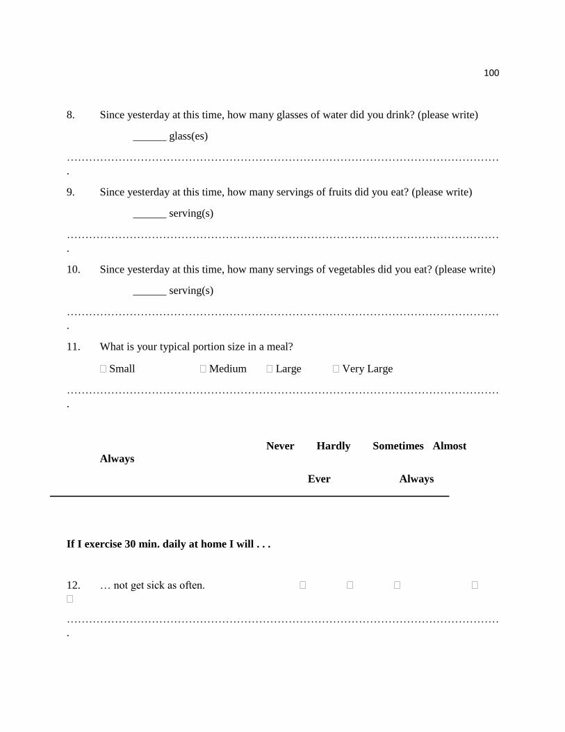
100

8. Since yesterday at this time, how many glasses of water did you drink? (please write)

______ glass(es)

………………………………………………………………………………………………………

.

9. Since yesterday at this time, how many servings of fruits did you eat? (please write)

______ serving(s)

………………………………………………………………………………………………………

.

10. Since yesterday at this time, how many servings of vegetables did you eat? (please write)

______ serving(s)

………………………………………………………………………………………………………

.

11. What is your typical portion size in a meal?

Small Medium Large Very Large

………………………………………………………………………………………………………

.

Never Hardly Sometimes Almost

Always

Ever Always

If I exercise 30 min. daily at home I will . . .

12. … not get sick as often.

………………………………………………………………………………………………………

.

101

13. …have more confidence.

………………………………………………………………………………………………………

.

14. …have more fun.

………………………………………………………………………………………………………

.

15. …look better.

………………………………………………………………………………………………………

.

If I watch TV less than 2 hours/day I will . . .

16. … have more friends.

………………………………………………………………………………………………………

.

17. …have more free time.

………………………………………………………………………………………………………

.

18. …have more fun.

………………………………………………………………………………………………………

.

102

19. …be more relaxed.

………………………………………………………………………………………………………

.

If I drink water instead of sweetened beverages I will . . .

20. … be more relaxed.

………………………………………………………………………………………………………

.

21. …feel better.

………………………………………………………………………………………………………

.

22. …have more energy.

………………………………………………………………………………………………………

.

23. …have better weight.

………………………………………………………………………………………………………

.

103

Never Hardly Sometimes Almost

Always

Ever Always

If I eat 5 or more servings of fruits and

vegetables I will . . .

24. … have more energy.

………………………………………………………………………………………………………

.

25. …feel better.

………………………………………………………………………………………………………

.

26. …not get sick as often.

………………………………………………………………………………………………………

.


………………………………………………………………………………………………………

.

If I eat smaller portion size I will…


104

………………………………………………………………………………………………………

.

29. …have more energy.

………………………………………………………………………………………………………

.

30. …feel better.

………………………………………………………………………………………………………

.

31. …be more relaxed.

………………………………………………………………………………………………………

.

Not at All- Slightly- Moderately -Very -Extremely

(Important)

How important is it to you that you . . .?

32. … not get sick as often?

………………………………………………………………………………………………………

.

33. …have more confidence?

………………………………………………………………………………………………………

.

34. …have more fun?

………………………………………………………………………………………………………

.

35. …look better?

………………………………………………………………………………………………………

.

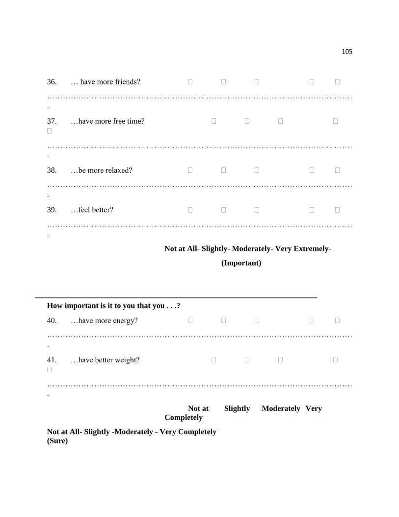
105

36. … have more friends?

………………………………………………………………………………………………………

.

37. …have more free time?

………………………………………………………………………………………………………

.

38. …be more relaxed?

………………………………………………………………………………………………………

.

39. …feel better?

………………………………………………………………………………………………………

.

Not at All- Slightly- Moderately- Very Extremely-

(Important)

How important is it to you that you . . .?

40. …have more energy?

………………………………………………………………………………………………………

.

41. …have better weight?

………………………………………………………………………………………………………

.

Not at Slightly Moderately Very

Completely

Not at All- Slightly -Moderately - Very Completely

(Sure)

106

How sure are you that you can . . .?

42. … exercise every day for

30 minutes at home?

………………………………………………………………………………………………………

.

43. … exercise for 30 minutes

at home even if you are tired?

………………………………………………………………………………………………………

.

44. … exercise for 30 minutes

at home even if you are busy?

………………………………………………………………………………………………………

.

45. … set goals to exercise every day for

30 minutes at home?

………………………………………………………………………………………………………

.

46. … reward yourself with

something you like for exercising?

………………………………………………………………………………………………………

.

47. … watch TV no more than

2 hours per day?

………………………………………………………………………………………………………

.

48. … reduce watching TV even if your

107

favorite shows are coming?

………………………………………………………………………………………………………

.

49. … reduce watching TV even if everyone

else in the family is watching?

………………………………………………………………………………………………………

.

50. … set goals to watch TV to no

more than 2 hours per day?

………………………………………………………………………………………………………

.


something you like for reducing

watching TV?

………………………………………………………………………………………………………

.

52. … drink more water?

………………………………………………………………………………………………………

.

53. … drink water every day

instead of sweet drinks?

………………………………………………………………………………………………………

.

54. … drink more water every day

even if you do not feel thirsty?

108

………………………………………………………………………………………………………

.

Not at all - Slightly -Moderately- Very- Completely

(SURE)

How sure are you that you can . . .?

55. … set goals to replace sweet drinks with

water every day?

………………………………………………………………………………………………………

.


something you like for drinking

water instead of sweet drinks?

………………………………………………………………………………………………………

.

57. …eat 5 or more servings of fruits and

vegetables every day?

………………………………………………………………………………………………………

.

58. …eat 5 or more servings of fruits and

vegetables every day even if you do not

like them?

109

………………………………………………………………………………………………………

.

59. … eat 5 or more servings of fruits and

vegetables every day even if others in your

family do not like them?

………………………………………………………………………………………………………

.

60. …set goals to eat 5 or more servings of

fruits and vegetables?

………………………………………………………………………………………………………

.

61. … reward yourself with something

you like for eating 5 or more servings

of fruits and vegetables every day?

………………………………………………………………………………………………………

.

62. …eat smaller portion sizes?

………………………………………………………………………………………………………

.

63. … eat smaller portion sizes even

when you are hungry?

………………………………………………………………………………………………………

.

64. … eat smaller portion sizes even

when family members force you to eat?

………………………………………………………………………………………………………

.

110

65. …set goals to eat smaller portion sizes?

………………………………………………………………………………………………………

.

66. … reward yourself with something you

like for eating smaller portion sizes?

………………………………………………………………………………………………………

.

Thank you for your time!

111

Appendix B: Student Assent Form

Hello, my name is Augustina Anyikwa and I am doing a research project to learn about Childhood

obesity and how we as community can help to prevent it. I am inviting you to join my project. I

am inviting all Hispanic American children attending this church from the ages of 11-15. Able to

understand, read, and /or write English to be in the study. I am going to read this form with your

leader to you. I want you to learn about the project before you decide if you want to be in it.

WHO I AM: I am a student at Walden University. I am working on my doctoral degree and I live

in DeKalb County.

ABOUT THE PROJECT: If you agree to be in this project, you will be asked to:

The study will be conducted once at the school, questionnaire will be read out to participants in

group if possible. To complete it might take lee than 30 minutes.

Researcher will meet with the participants that met the criteria in a designated area in the church.

Here are few sample questions:

African American or African American

Asian

American Indian

Hispanic American

Other _________________

…………………………………………………………………………………………………

…….

112

How old are you today?

Younger than 11 years old

12 years old

13 years old

14 years old

15 years old

16 years old

older than 16 years

………………………………………………………………………………………………

………

Are you a…? Boy

Girl

…………………………………………………………………………………………………

…….

How many times have you been taught in school about healthy eating?

Never

Once

Twice


…………………………………………………………………………………………………

…….

How many times have you been taught in school to do physical activity or exercise at

home?

Never

Once

Twice

113


IT’S YOUR CHOICE: You don’t have to be in this project if you don’t want to. If you decide now

that you want to join the project, you can still change your mind later. If you want to stop, you can.

Being in this project might make you tired or stressed, just like 30 minutes or more completing the

survey just one time. But we are hoping this project might help others by eating healthy and being

physically active may reduce the incidences of obesity and diseases that comes with it therefore

helping people to live longer and healthy.

No payment. There is no personal gain, but individual participants will be made aware how their

participation will assist in informing positive social change in prevention of childhood obesity in

the community.

PRIVACY:

Everything you tell me during this project will be kept private. That means that no one else will

know your name or what answers you gave. The only time I must tell someone is if I learn about

something that could hurt you or someone else.

ASKING QUESTIONS:

You can ask me any questions you want now. If you think of a question later, you or your parents

can reach me at 404 464 6925. If. If you or your parents would like to ask my university a question,

you can call 612-312-1210.

I will give you a copy of this form to keep.

114

If you want to join the project, please sign your name below.

Name

Signature

Date

Researcher Signature

115

IRB will enter approval number here and it expires on IRB will enter expiration date.

The researcher will give you a copy of this form to keep.

Obtaining Your Consent

If you feel you understand the study well enough to decide about it, please indicate your consent

by signing below.

Printed Name of Parent

Printed Name of Child

Date of consent

Parent’s Signature

Researcher’s Signature

116

Appendix C

Model Selection and Verification of Model Assumptions

Research Question 1

To what extent if any does select social construct theory predicts television-watching behavior


First a multiple linear regression model including all considered variable was used.

𝑌𝑡𝑠𝑡𝑣 = 𝛽0 + 𝛽𝑒𝑥𝑝𝑡𝑛𝑡𝑣 + 𝛽𝑠𝑒𝑙𝑓𝑒𝑡𝑣 + 𝛽𝑠𝑒𝑙𝑓𝑒𝑏𝑡𝑣 + 𝛽𝑠𝑒𝑙𝑓𝑒𝑐𝑡𝑣 + 𝛽𝑎𝑔𝑒 + 𝛽𝑔𝑒𝑛𝑑𝑒𝑟 + 𝛽𝑡𝑝𝑎2 + 𝛽𝑡ℎ𝑒2 + 𝜀𝑖

See appendix E for definition of variables.

Analysis of the regression output indicated that there is multicollinearity among the variables. The

variable with the strongest indicator of multicollinearity (selfebtv, vif=14.231) was then removed.

The categorical variables representing number times physical activities and healthy eating were

taught in school (tpa & the respectively) were binned into dichotomous variable due to sparse

responses (see descriptive below). Subsequently auto-variable selection tool in R was employed

to identity “best subset” model as Model 4 (see table 1 below).

Table A1

Best Subsets Regression

Model Index Predictors

1 exptntv

2 exptntv gender

3 exptntv gender tpa2

4 exptntv selfectv gender tpa2

5 exptntv selfectv gender tpa2 the2

117

6 exptntv selfectv age gender tpa2 the2

7 exptntv selfetv selfectv age gender tpa2 the2

Table A2

Subsets Regression Summary

Adj.

Model R-Square R- Square AIC SBIC SBC MSEP FPE HSP

APC

1 0.06 0.05 666.98 56.80 677.10 1.29 1.29 0.00 0.96

2 0.0777 0.0690 665.2421 55.15 678.72 1.28 1.28 0.00 0.95

3 0.0864 0.0734 665.2217 55.2202 682.0749 1.2805 1.2800 0.0060 0.9483

4 0.0977 0.0805 664.5320 54.6931 684.7558 1.2767 1.2759 0.0060 0.9453

5 0.1034 0.0819 665.1771 55.4767 688.7715 1.2809 1.2798 0.0060 0.9481

6 0.1046 0.0788 666.8853 57.2788 693.8504 1.2915 1.2900 0.0060 0.9557

7 0.1047 0.0744 668.8700 59.3418 699.2058 1.3040 1.3020 0.0061 0.9645

The resulting model below (model 4) has variables with VIF all less than 2 and was adopted as

final model for research question 1.

Final model for research question1:

𝑌𝑡𝑠𝑡𝑣 = 𝛽0 + 𝛽𝑒𝑥𝑝𝑡𝑛𝑡𝑣 + 𝛽𝑠𝑒𝑙𝑓𝑒𝑐𝑡𝑣 + 𝛽𝑔𝑒𝑛𝑑𝑒𝑟 + 𝛽𝑡𝑝𝑎2 + 𝜀𝑖


Testing model assumptions for research question 1:

The selected final model was tested for key assumptions of multiple linear regressions. The figures

below indicated that deviation from expected perfect outcome was not to the extent that will affect

the validity of results. The plot of residual vs. fitted values (fig. 1) indicated that the assumptions

118

of constant variance was not violated. There was no

discernable pattern in these plots and the fitted line seem horizontal indicating that the variance

does not change significantly as data value increases. Fig. 2 indicated that deviation from

normality was not severe and considered adequate with n=215.

Using 2 hrs. of television watching as demarcation, the logistic regression model below was

subsequently used to investigate the relationship between select social construct theory and

probability of watching television 2 hrs. between males and females.

𝑙𝑜𝑔 [𝑝

1 − 𝑝] = 𝛽0 + 𝛽𝑔𝑒𝑛𝑑𝑒𝑟 + 𝜀𝑖

where p is the probability that the participant watched television for 2 hrs or more within the last

24 hours. Test for model fit for logistics regression was conducted by comparing the null and

deviance residual using logistic model above indicated that the model is appropriate (X2(1) =7.33,

P= 0.0068).

Research Question 2

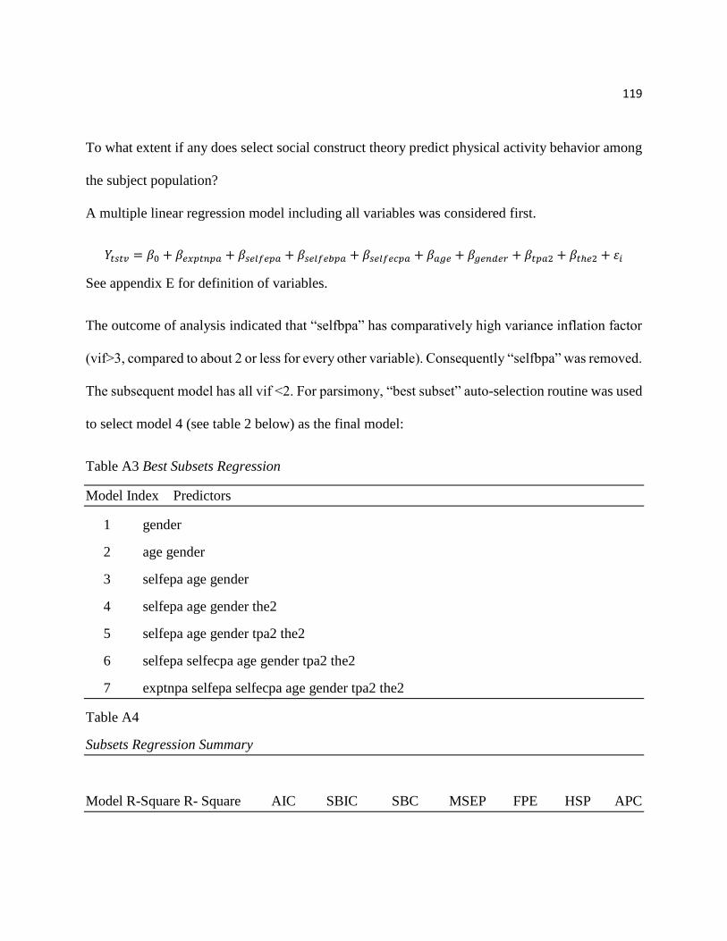
119

To what extent if any does select social construct theory predict physical activity behavior among


A multiple linear regression model including all variables was considered first.

𝑌𝑡𝑠𝑡𝑣 = 𝛽0 + 𝛽𝑒𝑥𝑝𝑡𝑛𝑝𝑎 + 𝛽𝑠𝑒𝑙𝑓𝑒𝑝𝑎 + 𝛽𝑠𝑒𝑙𝑓𝑒𝑏𝑝𝑎 + 𝛽𝑠𝑒𝑙𝑓𝑒𝑐𝑝𝑎 + 𝛽𝑎𝑔𝑒 + 𝛽𝑔𝑒𝑛𝑑𝑒𝑟 + 𝛽𝑡𝑝𝑎2 + 𝛽𝑡ℎ𝑒2 + 𝜀𝑖


The outcome of analysis indicated that “selfbpa” has comparatively high variance inflation factor

(vif>3, compared to about 2 or less for every other variable). Consequently “selfbpa” was removed.

The subsequent model has all vif <2. For parsimony, “best subset” auto-selection routine was used

to select model 4 (see table 2 below) as the final model:

Table A3 Best Subsets Regression


1 gender

2 age gender

3 selfepa age gender

4 selfepa age gender the2

5 selfepa age gender tpa2 the2

6 selfepa selfecpa age gender tpa2 the2

7 exptnpa selfepa selfecpa age gender tpa2 the2

Table A4


Model R-Square R- Square AIC SBIC SBC MSEP FPE HSP APC

120

1 0.1113 0.1071 1777.6889 1166.9751 1787.8008 226.1568 226.1372 1.0569

0.9054

2 0.1919 0.1842 1759.2546 1148.8231 1772.7371 207.6013 207.5561 0.9701

0.8310

3 0.2360 0.2251 1749.1864 1139.1048 1766.0396 198.1387 198.0612 0.9259

0.7930

4 0.2574 0.2433 1745.0596 1135.2823 1765.2835 194.4148 194.2965 0.9085

0.7779

5 0.2585 0.2407 1746.7576 1137.0713 1770.3521 196.0087 195.8382 0.9160

0.7841

6 0.2586 0.2372 1748.7192 1139.1122 1775.6843 197.8671 197.6349 0.9247

0.7913

7 0.2587 0.2336 1750.6958 1141.1676 1781.0316 199.7664 199.4625 0.9335

0.7986

Final model for research question 2:

𝑌𝑡𝑠𝑝𝑎 = 𝛽𝑠𝑒𝑙𝑓𝑒𝑝𝑎 + 𝛽𝑎𝑔𝑒 + 𝛽𝑔𝑒𝑛𝑑𝑒𝑟 + 𝛽𝑡ℎ𝑒2 + 𝜀𝑖

Testing model assumptions for research question 2:

The selected final model was tested for key assumptions of multiple linear regressions. The figures

below indicated that deviation from expected perfect outcome was not to the extent that will affect

the validity of results. The plot of residual vs. fitted values (fig. 3) indicated that the assumptions

of constant variance was not violated. There was no discernable pattern in these plots and the fitted

line seem more or less horizontal indicating that the variance does not change significantly as data

value increases.

121

Fig. 4 indicated that deviation from normality was not too severe and considered adequate with

n=215.

Using 30 minutes of exercise as demarcation, the logistic regression model below was used to

investigate the relationship between select social construct theory and probability of exercising

30min or more between males and females

𝑙𝑜𝑔 [𝑝

1 − 𝑝] = 𝛽0 + 𝛽𝑔𝑒𝑛𝑑𝑒𝑟 + 𝜀𝑖

where p is the probability that the participant exercised 30min or more within the last 24 hours.

Test for model fit for logistics regression was conducted by comparing the null and

deviance residual using logistic model above indicated that the model is appropriate (X2(1) =28.3,

P<0.0001).

Fig 3 Fig 4

122

Research Question 3

To what extent if any does select social construct theory predict water consumption among the

subject population?

In order to address this question, a multiple linear regression model including all variables of

interest was considered first.


See Appendix E for definition of variables.

The outcome of analysis indicated that “selfebdw” has the highest variance inflation factor

(vif>12). Consequently “selfebdw” was removed. The resulting model has all vif <3. “best subset”

auto-selection routine was used to select model 5 (see table 3 below) as the final model:

Table A5



123

1 selfecdw

2 selfecdw age

3 selfedw selfecdw age

4 selfecdw age tpa2 the2

5 selfedw selfecdw age tpa2 the2

6 exptndw selfedw selfecdw age tpa2 the2

7 exptndw selfedw selfecdw age gender tpa2 the2


Adj.


1 0.2161 0.2124 722.4246 111.9919 732.5365 1.6703 1.6702 0.0078 0.7987

2 0.2416 0.2345 717.2931 106.9157 730.7757 1.6312 1.6308 0.0076 0.7798

3 0.2594 0.2489 714.1913 103.9240 731.0444 1.6081 1.6074 0.0075 0.7687

4 0.2729 0.2591 712.2309 102.1164 732.4547 1.5938 1.5929 0.0074 0.7617

5 0.2909 0.2739 708.8582 99.0524 732.4527 1.5694 1.5681 0.0073 0.7498

6 0.2951 0.2748 709.5629 99.8999 736.5280 1.5751 1.5732 0.0074 0.7523

7 0.2979 0.2742 710.7025 101.1743 741.0382 1.5840 1.5816 0.0074 0.7563

Final model for research question 3

𝑌𝑔𝑜𝑤 = 𝛽𝑠𝑒𝑙𝑓𝑒𝑑𝑤 + 𝛽𝑠𝑒𝑙𝑓𝑒𝑐𝑑𝑤 + 𝛽𝑎𝑔𝑒 + 𝛽𝑡𝑝𝑎2 + 𝛽𝑡ℎ𝑒2 + 𝜀𝑖

124

Testing Model Assumptions for Research Question 3:

The selected final model was tested for key assumptions of multiple linear regressions. The

figures below indicated that deviation from expected perfect outcome was not to the extent that

will affect the validity of results. The plot of residual vs. fitted values (fig. 6) indicated that the

assumptions of constant variance was not violated. There was no discernable pattern in these plots

and the fitted line seem horizontal indicating that the variance does not change significantly as

data value increases. Fig. 7 indicated that deviation from normality was not severe and considered

adequate with n=215.

125

Figure 6 Figure 7

Logistic regression model was not implemented for research question 3 because all responses were

below the demarcation value of eight glasses of water.

Research Question 4

To what extent if any does select social construct theories predict fruit and vegetable intake among


Multiple linear regression model including all variables of interest was considered first.



Fig 7

126

The outcome of initial analysis indicated that “selfebsofv” has the highest variance inflation factor

(vif>22). Consequently “selfebsofv” was removed. In the resulting model, “selfesofv” has

comparatively high vif (>5) and was subsequently removed. Thereafter, “best subset” auto-

selection routine was used to select model 4 (see Table 4) as the final model:

Table A6



1 selfecsofv

2 selfecsofv age

3 exptnsofv selfecsofv age

4 exptnsofv selfecsofv age gender

5 exptnsofv selfecsofv age gender tpa2

6 exptnsofv selfecsofv age gender tpa2 the2


Adj.


1 0.2035 0.1997 928.6105 318.0021 938.7224 4.3581 4.3577 0.0204 0.8115

2 0.2615 0.2545 914.3531 303.9647 927.8356 4.0790 4.0781 0.0191 0.7594

3 0.2854 0.2752 909.2802 299.0712 926.1334 3.9846 3.9830 0.0186 0.7417

4 0.3020 0.2887 906.2048 296.2160 926.4287 3.9288 3.9264 0.0184 0.7312

5 0.3125 0.2961 904.9500 295.1767 928.5444 3.9070 3.9036 0.0183 0.7269

6 0.3143 0.2945 906.4011 296.7264 933.3662 3.9347 3.9301 0.0184 0.7319

Final model for research question 4

127

𝑌𝑠𝑜𝑓𝑣 = 𝛽0 + 𝛽𝑒𝑥𝑝𝑡𝑛𝑠𝑜𝑓𝑣 + 𝛽𝑠𝑒𝑙𝑓𝑒𝑐𝑠𝑜𝑓𝑣 + 𝛽𝑎𝑔𝑒 + 𝛽𝑔𝑒𝑛𝑑𝑒𝑟 + 𝜀𝑖


Testing Model Assumptions for Research Question 4:

The selected final model was tested for key assumptions of multiple linear regressions. The

figures below indicated that deviation from expected perfect outcome was not to the extent that

will affect the validity of results. The plot of standardized residual vs. fitted values (fig. 8) indicated

that the assumptions of constant variance was not severely violated. There was no discernable

pattern in these plots and the fitted line seem horizontal, apart from lower predicted values,

indicating that the variance does not change significantly as data value increases. Fig. 9 indicated

there is deviation from normality, simple transformations (log and square root of response

variable) did not adequately correct this deviation from normality. However, given fairly large

sample size (n=215), we know that by central limit theorem, the inference will still yield relatively

valid result.

128

Figure 9

Figure 8

A logistic regression model could not be implemented for research question 4 because

only four of the responses were above the demarcation value of 5 servings of fruit and 5

servings of vegetable.

Research Question 5

To what extent if any does select social construct theory predict portion size among the subject

population? The number of respondents whose typical meal portion size are small or very large

were both less than 5 (4 & 3 respectively). Meal portion size was therefore binned to create a

dichotomous variable (small or medium=0, and large or very large = 1). The following model was

used to analysis the data:

Fig 9

Fig 8

129

𝑙𝑜𝑔 [𝑝

1 − 𝑝] = 𝛽0 + 𝛽𝑒𝑥𝑝𝑡𝑛𝑠𝑝𝑠 + 𝛽𝑠𝑒𝑙𝑓𝑒𝑠𝑝𝑠 + 𝛽𝑠𝑒𝑙𝑓𝑒𝑏𝑠𝑝𝑠 + 𝛽𝑠𝑒𝑙𝑓𝑒𝑐𝑠𝑝𝑠 + 𝛽𝑎𝑔𝑒 + 𝛽𝑔𝑒𝑛𝑑𝑒𝑟 + 𝛽𝑡𝑝𝑎2 + 𝛽𝑡ℎ𝑒2

+ 𝜀𝑖

where p is the probability that the participant’s typical meal portion size is large or very large

Test for logistic regression model fit:

Test for model fit for logistics regression was conducted by comparing the null and deviance

residual using logistic model above indicated that the model is appropriate (X2(8) =52.4, P

<0.0001).

Appendix D: Code Book

HEALTH FOR ALL

Promoting Healthy Lifestyles: Survey

s/n Variable Name &

Description

Variable name

(coding)

Data Type Format

1 Age: Students age,

ranging from less than 11

to more than 16yrs

Age Categorical Ordinal: >11yrs,

12yrs, 13yrs,

14yrs, 15yrs,

16yrs, >16yrs

130

2 Gender: Male /female Sex Categorical Nominal: male=1,

female=0

3 Race: African American

refers to African

American or African

American, Indian refers to

Indian American

Race Categorical Nominal:

Caucasian=1,

African

American=2,

Hispanic

American=3,

Asian=4,

Indian=5, other=6

4 Taught about healthy

eating: number of times

students were taught in

school the past one week.

the (the2=binary

coding

2orless|>2)

Categorical Ordinal: Never=0,

once=1, twice=2,

three or more

times=3

5 Taught about physical

activity or exercise:

number of times students

were taught in school the

past one week.

tpa (tpa2=binary

coding

2orless|>2)

Categorical Ordinal: Never=0,

once=1, twice=2,

three or more

times=3

6 Time spent on physical

activity or exercise in

past 24 hours

tspa

(tspa2=binary

coding)

Numerical Continuous

/categorical

variable

Less than 30 min

(0), 30min or

more (1)

7 Time spent watching TV

in past 24 hours

tstv (tstv2=binary

coding)

Numerical Continuous

/categorical

variable

Less than 2 hrs

(0), 2 hrs or more

(1)

131

8 Glasses of water:

Number of glasses of

water student drank in the

past 24 hours

Gow Numerical Continuous

/categorical

variable

Less than 8

glasses (0), 8

glasses or more

(1)

9 Servings of fruit:

Number of servings of

fruit student ate in the past

24 hours

Sof Numerical Continuous

/categorical

variable

Less than 5

servings (0), 5

servings or more

(1)

10 Servings of vegetable:

Number of servings of

vegetable student ate in

the past 24 hours

Sov Numerical Continuous

/categorical

variable

Less than 5

servings (0), 5

servings or more

(1)

10b Total Servings of fruits

& vegetable: Total

number of servings of

fruits and vegetable

student ate in the past 24

hours

Sofv Numerical Continuous

11 Meal Portion size:

Students typical meal

portion size

Mps (mps2) Categorical Ordinal: small =1,

medium=2,

large=3, very

large=4 [for

mps2: small or

medium =0 while

132

large or very

large=1]

Motivation (mpa): If I exercise 30 min. daily at home I will . . .

12 …not get sick as often mpa_12 Likert Scale Scale of 0 to 4:

Never=0, Hardly

ever=1,

Sometimes=2,

Almost

Always=3,

Always=4

13 …have more confidence mpa_13 Likert Scale Scale of 0 to 4:

Never=0, Hardly

ever=1,

Sometimes=2,

Almost

Always=3,

Always=4

14

…have more fun

mpa_14

Likert Scale

Scale of 0 to 4:

Never=0, Hardly

ever=1,

Sometimes=2,

Almost

Always=3,

Always=4

15 …look better mpa_15 Likert Scale Scale of 0 to 4:

Never=0, Hardly

ever=1,

Sometimes=2,

Almost

Always=3,

Always=4

133

Motivation (mtv) If I watch TV less than 2 hours/day I will...

16 … have more friends. mtv_16 Likert Scale Scale of 0 to 4:

Never=0, Hardly

ever=1,

Sometimes=2,

Almost

Always=3,

Always=4

17 …have more free time. mtv_17 Likert Scale Scale of 0 to 4:

Never=0, Hardly

ever=1,

Sometimes=2,

Almost

Always=3,

Always=4

18 …have more fun. mtv_18 Likert Scale Scale of 0 to 4:

Never=0, Hardly

ever=1,

Sometimes=2,

Almost

Always=3,

Always=4

19 …be more relaxed. mtv_19 Likert Scale Scale of 0 to 4:

Never=0, Hardly

ever=1,

Sometimes=2,

Almost

Always=3,

Always=4

Motivation (mgow): If I drink water instead of sweetened beverages I will . . .

20 …be more relaxed. mgow_20 Likert Scale Scale of 0 to 4:

Never=0, Hardly

ever=1,

Sometimes=2,

Almost

134

Always=3,

Always=4

21 …feel better. mgow_21 Likert Scale Scale of 0 to 4:

Never=0, Hardly

ever=1,

Sometimes=2,

Almost

Always=3,

Always=4

22 …have more energy. mgow_22 Likert Scale Scale of 0 to 4:

Never=0, Hardly

ever=1,

Sometimes=2,

Almost

Always=3,

Always=4

23 …have better weight. mgow_23 Likert Scale Scale of 0 to 4:

Never=0, Hardly

ever=1,

Sometimes=2,

Almost

Always=3,

Always=4

Motivation (msov): If I eat 5 or more servings of fruits and vegetables I will .

. .

24 … have more energy. msov_24 Likert Scale Scale of 0 to 4:

Never=0, Hardly

ever=1,

Sometimes=2,

Almost

Always=3,

Always=4

25 …feel better. msov_25 Likert Scale Scale of 0 to 4:

Never=0, Hardly

135

ever=1,

Sometimes=2,

Almost

Always=3,

Always=4

26 …not get sick as often. msov_26 Likert Scale Scale of 0 to 4:

Never=0, Hardly

ever=1,

Sometimes=2,

Almost

Always=3,

Always=4

27 …have better weight. msov_27 Likert Scale Scale of 0 to 4:

Never=0, Hardly

ever=1,

Sometimes=2,

Almost

Always=3,

Always=4

Motivation (mmps): If I eat smaller portion size I will…

28 …have better weight. mmps_28 Likert Scale Scale of 0 to 4:

Never=0, Hardly

ever=1,

Sometimes=2,

Almost

Always=3,

Always=4

29 …have more energy.

mmps_29 Likert Scale Scale of 0 to 4:

Never=0, Hardly

ever=1,

Sometimes=2,

Almost

Always=3,

Always=4

136

30 …feel better. mmps_30 Likert Scale Scale of 0 to 4:

Never=0, Hardly

ever=1,

Sometimes=2,

Almost

Always=3,

Always=4

31 …be more relaxed. mmps_31 Likert Scale Scale of 0 to 4:

Never=0, Hardly

ever=1,

Sometimes=2,

Almost

Always=3,

Always=4

Motivation (mimp): How important is it to you that you . . .

32 … not get sick as often?

mimp_32 Likert Scale Scale of 0 to 4:

Not at All

important=0,

Slightly important

= 1, Moderately

important = 2,

Very important =

3,Extremely

Important =4

33 …have more

confidence?


Not at All

important=0,

Slightly important

= 1, Moderately

important = 2,

Very important =

3, Extremely

Important =4

34 …have more fun? mimp_34 Likert Scale Scale of 0 to 4:

Not at All

important=0,

Slightly important

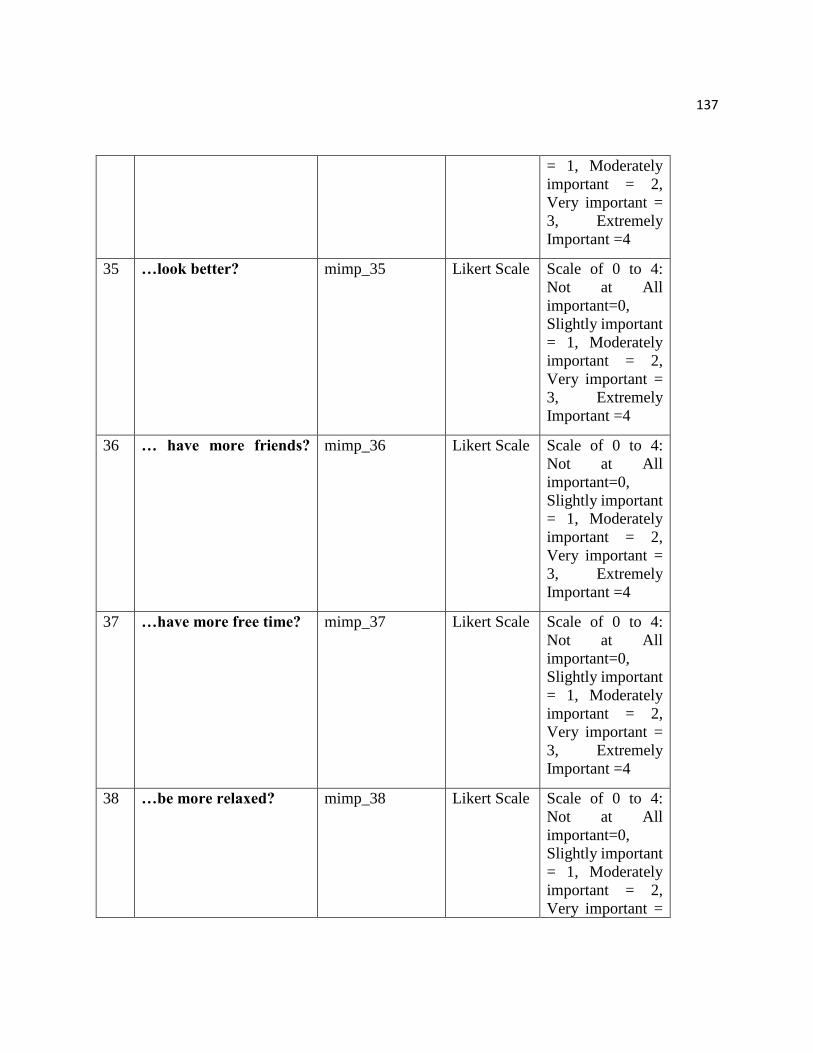
137

= 1, Moderately

important = 2,

Very important =

3, Extremely

Important =4

35 …look better? mimp_35 Likert Scale Scale of 0 to 4:

Not at All

important=0,

Slightly important

= 1, Moderately

important = 2,

Very important =

3, Extremely

Important =4

36 … have more friends?


Not at All

important=0,

Slightly important

= 1, Moderately

important = 2,

Very important =

3, Extremely

Important =4

37 …have more free time? mimp_37 Likert Scale Scale of 0 to 4:

Not at All

important=0,

Slightly important

= 1, Moderately

important = 2,

Very important =

3, Extremely

Important =4

38 …be more relaxed? mimp_38 Likert Scale Scale of 0 to 4:

Not at All

important=0,

Slightly important

= 1, Moderately

important = 2,

Very important =

138

3, Extremely

Important =4

39 …feel better? mimp_39 Likert Scale Scale of 0 to 4:

Not at All

important=0,

Slightly important

= 1, Moderately

important = 2,

Very important =

3, Extremely

Important =4

40 …have more energy mimp_40 Likert Scale Scale of 0 to 4:

Not at All

important=0,

Slightly important

= 1, Moderately

important = 2,

Very important =

3, Extremely

Important =4

41 …have better weight? mimp_41 Likert Scale Scale of 0 to 4:

Not at All

important=0,

Slightly important

= 1, Moderately

important = 2,

Very important =

3, Extremely

Important =4

Motivation (msure): How sure are you that you can . . .

42 … exercise every day for

30 minutes at home?

msure_42 Likert Scale Scale of 0 to 4:

Not at all sure =0,

Slightly sure= 1,

Moderately sure =

2, Very sure = 3,

Completely sure =

4

139

43 … exercise for 30 minutes

at home even if you are

tired?


Not at all sure =0,

Slightly sure= 1,

Moderately sure =

2, Very sure = 3,

Completely sure =

4

44 … exercise for 30 minutes

at home even if you are

busy?


Not at all sure =0,

Slightly sure= 1,

Moderately sure =

2, Very sure = 3,

Completely sure =

4

45 … set goals to exercise

every day for 30 minutes

at home?


Not at all sure =0,

Slightly sure= 1,

Moderately sure =

2, Very sure = 3,

Completely sure =

4

46 … reward yourself with

something you like for

exercising?


Not at all sure =0,

Slightly sure= 1,

Moderately sure =

2, Very sure = 3,

Completely sure =

4

47 … watch TV no more than

2 hours per day?


Not at all sure =0,

Slightly sure= 1,

Moderately sure =

2, Very sure = 3,

Completely sure =

4

48 … reduce watching TV

even if your favorite

shows are coming?


Not at all sure =0,

Slightly sure= 1,

140

Moderately sure =

2, Very sure = 3,

Completely sure =

4

49 … reduce watching TV

even if everyone else in

the family is watching?


Not at all sure =0,

Slightly sure= 1,

Moderately sure =

2, Very sure = 3,

Completely sure =

4

50 … set goals to watch TV

to no more than 2 hours

per day?


Not at all sure =0,

Slightly sure= 1,

Moderately sure =

2, Very sure = 3,

Completely sure =

4



reducing watching TV?


Not at all sure =0,

Slightly sure= 1,

Moderately sure =

2, Very sure = 3,

Completely sure =

4

52 … drink more water? msure_52 Likert Scale Scale of 0 to 4:

Not at all sure =0,

Slightly sure= 1,

Moderately sure =

2, Very sure = 3,

Completely sure =

4

53 … drink water every day

instead of sweet drinks?


Not at all sure =0,

Slightly sure= 1,

Moderately sure =

2, Very sure = 3,

141

Completely sure =

4

54 … drink more water every

day even if you do not feel

thirsty?


Not at all sure =0,

Slightly sure= 1,

Moderately sure =

2, Very sure = 3,

Completely sure =

4

55 … set goals to replace

sweet drinks with water

every day?


Not at all sure =0,

Slightly sure= 1,

Moderately sure =

2, Very sure = 3,

Completely sure =

4



drinking water instead of

sweet drinks?


Not at all sure =0,

Slightly sure= 1,

Moderately sure =

2, Very sure = 3,

Completely sure =

4

57 …eat 5 or more servings

of fruits and

vegetables every day?


Not at all sure =0,

Slightly sure= 1,

Moderately sure =

2, Very sure = 3,

Completely sure =

4

58 …eat 5 or more servings

of fruits and

vegetables every day even

if you do not

like them?


Not at all sure =0,

Slightly sure= 1,

Moderately sure =

2, Very sure = 3,

Completely sure =

4

142

59 … eat 5 or more servings

of fruits and

vegetables every day even

if others in your

family do not like them?


Not at all sure =0,

Slightly sure= 1,

Moderately sure =

2, Very sure = 3,

Completely sure =

4

60 …set goals to eat 5 or

more servings of

fruits and vegetables?


Not at all sure =0,

Slightly sure= 1,

Moderately sure =

2, Very sure = 3,

Completely sure =

4


something

you like for eating 5 or

more servings

of fruits and vegetables

every day?


Not at all sure =0,

Slightly sure= 1,

Moderately sure =

2, Very sure = 3,

Completely sure =

4

62 …eat smaller portion

sizes?


Not at all sure =0,

Slightly sure= 1,

Moderately sure =

2, Very sure = 3,

Completely sure =

4

63 … eat smaller portion

sizes even when you are

hungry?


Not at all sure =0,

Slightly sure= 1,

Moderately sure =

2, Very sure = 3,

Completely sure =

4

143

64 … eat smaller portion

sizes even when family

members force you to eat?


Not at all sure =0,

Slightly sure= 1,

Moderately sure =

2, Very sure = 3,

Completely sure =

4

65 …set goals to eat smaller

portion sizes?


Not at all sure =0,

Slightly sure= 1,

Moderately sure =

2, Very sure = 3,

Completely sure =

4


something you

like for eating smaller

portion sizes?


Not at all sure =0,

Slightly sure= 1,

Moderately sure =

2, Very sure = 3,

Completely sure =

4

using social cognitive theory to predict obesity behaviors

Documents