W. J. Usery Workplace Research Group Paper Series

Working Paper 2016-8-1

August 2016

Using Spatial Factor Analysis to Measure Human Development

Qihua Qiu

Georgia State University

Jaesang Sung

Georgia State University Will Davis

Georgia State University Rusty Tchernis Georgia State University, IZA, and NBER This paper can be downloaded at: http://uwrg.gsu.edu

ANDREW YOUNG SCHOOL

O F P O L I C Y S T U D I E S

1

Using Spatial Factor Analysis to Measure Human

Development1

Qihua Qiu†, Jaesang Sung†, Will Davis†, and Rusty Tchernis†,§

†Department of Economics, Georgia State University

§IZA & NBER

August 18, 2016

Abstract

In this paper, we propose a Bayesian factor analysis model with the purpose of serving as an

alternate approach to calculating the UNDP’s Human Development Index, as well as providing a

general methodology which can be used to augment existing indices or build new ones. In

addition to addressing several potential issues of the official HDI, we also estimate an alternative

“green HDI” index by adding a new environmental variable, and build a novel MDG index as an

example of constructing a new index with a more complex variable structure. Under our

methodology, we find the “living standard” dimension provides a greater proportional

contribution to human development than it is assigned by the official HDI while the “longevity”

dimension provides a lower proportional contribution. The results also show considerable levels

of general disagreement when compared to the ranks of the official HDI. We show that

incorporating an environmental variable increases the amount of disagreement between model

based ranks and the official HDI, but decreases the amount of uncertainty associated with model

ranks. In addition, we report the sensitivity of our methods to the choice of functional form and

data imputation procedures.

Keywords: Human Development Index, factor analysis

JEL Classification: O15, O57

1 We would like to thank Spencer Banzhaf, Alberto Chong and Andrew Foster for valuable comments and

suggestions. Address correspondence to Qihua Qiu, qqiu@student.gsu.edu, Department of Economics, Georgia

State University, Atlanta GA 30303.

2

1. Introduction

Designed as a ranking system to track global human development, the Human Development

Index (HDI) was first introduced in 1990 by the United Nations Development Programme

(UNDP) in their now long running series of annual Human Development Reports (HDR). Prior

to the HDI’s initial publication, GDP, GDP per capita, and GNP had long served as the primary

indicators of development for academics, policymakers, and other interested parties; but each

lacked something the UNDP saw as vital to fully understanding global development - the human

factor. Defined by the first HDR as, “…the process of enlarging people’s choices” (UNDP,

1990), human development is simply any method by which nations expand or strengthen their

citizens’ access to human capital building resources. Based on this notion, the HDI formulates its

national ranks using three key indicators which are believed to be connected to a country’s

human development level: longevity, education, and decency of living standards.2

In the years since its introduction, the HDI has come to serve as the standard for government

agencies, private industry professionals, development groups, and academic researchers

interested in studying and comparing national levels of human development. During a session in

2006, the National Congress of Indonesian Human Development restated their use of HDI as an

economic indicator of development outcomes and the satisfaction of basic human living needs

(Fattah and Muji, 2012). The government of Ireland also provides more development aid to

countries classified as “low human development” by the HDI (O’Neill, 2005; Wolff et al., 2011).

In private industry, the pharmaceutical company Merck sells drugs at a significant discount to

nearly all of the countries categorized as “low human development” (Petersen and Rother, 2001;

Wolff et al., 2011). Additionally, there have been proposals when designing international climate

2 For a more detailed account of the rationale behind the design of the first HDI, see Anand and Sen (1994).

3

change policy that each country’s HDI ranking should be factored into their reduction

obligations for greenhouse gas emissions (Hu, 2009; Wolff et al., 2011). In research, the HDI is

widely used as an alternative to other traditional economic indicators when evaluating a nation’s

relative level of human development (Anand and Ravallion, 1993; Easterlin, 2000). Furthermore,

the HDI is not only heavily utilized by economists and other social scientists, but a wide array of

academic disciplines including the medical research community.3

With the HDI’s position as a top index now solidified through time and use, it serves as an

advantageous exercise to reevaluate its formulation. When studied critically, the HDI does have

a number of potential issues which we seek to address. Each of the three indicators used to

calculate the official HDI are assigned deterministic weights relating to the proportional

contribution they are assumed to provide towards a nation’s human development level.

Additionally, the HDI does not incorporate a measure of uncertainty in their rankings; implying

that each publication of the official HDI can be interpreted as only one of many potential

rankings. A considerable number of previous studies have attempted to address these and similar

concerns with potential methods to correct for deterministic weights across dimensions

(Ravallion, 2012), and lack of uncertainty from measurement error, index structure, and formula

volatility (Noorbakhsh, 1998; Morse, 2003a; Wolff et al., 2009). Abayomi and Pizarro (2013)

take a Bayesian framework to generate the confidence intervals of the HDI with the goal of

incorporating uncertainty by first assuming prior distributions of both the underlying data and

variable weights, and then examining the posterior replicates. An even more relevant study to our

paper, Hoyland et al. (2012) also adopt a Bayesian factor analysis model; but it differs from our

3 For instance, the relationship between the HDI and health has extensively been studied in topics such as: cancer (Bray et al.,

2012), infant and maternal death (Lee et al., 1997), depressive episodes (Cifuentes et al., 2008), kidney cancer incidents and

incident-to-mortality rates (Patel et al., 2012), suicide (Shah, 2009), and prevalence of physical inactivity (Dumith et al., 2011).

4

methodology in that they allow for correlations among indicators by first assuming correlations

among the factor loadings of the HDI’s four manifest variables.

This paper adopts a Bayesian factor analysis model which was initially developed to address

many of the same concerns present in the material deprivation index (Hogan and Tchernis,

2004).4 The model assumes an underlying latent variable, a factor representing levels of human

development, which is manifested in the observed measures. The factor is influenced by the

observed variables, and the strength of this influence is computed strictly from the data as

opposed to expert opinion. The results of our model are summarized by computing the posterior

distribution of ranks for all countries which are then presented with confidence intervals. This

gives a more comprehensive view of a nation’s standing relative to its peers given the inherent

uncertainty of the estimation process. To further reduce the uncertainty of our measurements, we

also include measures of spatial correlation and national population. Spatial correlation is often

used in related literature as it allows for the incorporation of potential spillover effects from other

factors which are highly correlated with HDI (Eberhardt et al. 2013; Ertur and Koch, 2011;

Conley and Ligon, 2002; Keller, 2002).5

We illustrate the flexibility of our model to the inclusion of additional data in two ways. First,

we add a measure of environmental sustainability to the HDI. Common candidates used as

environmental variables are resource consumption, such as a nation’s net natural capital stock

(Neumayer, 2001; Morse, 2003b), and pollution levels, which we see in prior literature using

CO2 emissions per capita. To construct our “green HDI”, we also use CO2 emissions per capita as

4 The same model has also been adopted in the measurement of county health rankings for Wisconsin and Texas (Courtemanche

et al., 2015). 5 The spatial dependence of HDI is based on prior literature. Research and development or long-run economic growth, both of

which could be correlated with each factor of the index, has the documented potential for international spillovers (Eberhardt et al.

2013; Ertur and Koch, 2011; Conley and Ligon, 2002; Keller, 2002). Additionally, Malczewski (2010) shows that there are

statistically significant geographical groups of high and low life expectancies in Poland.

5

it is recommended by the UNDP for the purposes of international analysis (Fuentes-Nieva and

Pereira, 2010). Second, our general method is also easily utilized when trying to construct new

indices as well. To exemplify the process of formulating a completely novel index, we construct

an “MDG index” using data from the United Nations Millennium Development Goals (MDG).6

Since the MDG’s primary purpose was to track global development progress overtime, it can be

interpreted as an alternative measure of human development to the HDI. Given the complex and

decentralized nature of the MDG’s design, a considerable quantity of prior research also attempts

to construct an index summarizing information presented by the MDG’s targets (Alkire and

Santos, 2010; De Muro et al. 2011; Abayomi and Pizarro, 2013).

2. Methods

Methods of the official HDI

As a precursor to discussing our methods, it is of use to summarize the methodology used by the

UNDP to formulate the official HDI. Since 2010, the HDI has constructed its three development

indicators using four manifest variables: life expectancy at birth (longevity), mean years of

schooling (education), expected years of schooling (education), and purchasing power-adjusted

real GNI per capita (living standard). 7

6 Established in 2000, the MDG are a set of eight development goals which the United Nations member countries committed to

achieve by the year 2015. 7 Since its introduction in 1990, the HDI has seen several alterations to its formulation. Some changes have been minor, but a

considerable overhaul was done in 2010. Prior to 2010, the four variables used to construct HDI were life expectancy at birth

(longevity), adult literacy rate (education), combined educational enrollment (education), and purchasing power-adjusted real GDP per capita (living standard). Three normalized indicators (longevity, education, living standard) are calculated from the four

variables. A simple average of the three indicators is scaled to range from 0 to 1 to represent the HDI score.

6

First, the three indicators are derived and normalized using the HDI’s four observed variables.

These indicators are the Life Expectancy Index (LEI), Education Index (EI), and Income Index

(II). Each indicator is constructed using the following method:

𝐿𝑖𝑓𝑒 𝐸𝑥𝑝𝑒𝑐𝑡𝑎𝑛𝑐𝑦 𝐼𝑛𝑑𝑒𝑥(𝐿𝐸𝐼) =𝐿𝐸 − 20

85 − 20

𝐸𝑑𝑢𝑐𝑎𝑡𝑖𝑜𝑛 𝐼𝑛𝑑𝑒𝑥(𝐸𝐼) =𝑀𝑌𝑆𝐼 + 𝐸𝑌𝑆𝐼

2

𝑀𝑌𝑆𝐼 =𝑀𝑌𝑆

15 , 𝐸𝑌𝑆𝐼 =

𝐸𝑌𝑆

18

𝐼𝑛𝑐𝑜𝑚𝑒 𝐼𝑛𝑑𝑒𝑥 (𝐼𝐼) =ln(𝐺𝑁𝐼𝑝𝑐) − ln(100)

ln(75,000 ) − ln(100)

After calculating the three indicators, the indicators’ geometric mean is found using the formula

below:

𝐻𝐷𝐼 = √𝐿𝐸𝐼 ∗ 𝐸𝐼 ∗ 𝐼𝐼3

With this algorithm, the UNDP is able to guarantee that each HDI score will fall into the

range of values from 0 to 1. Following the designation of each nation’s raw HDI score, countries

are both ranked and categorized into one of the following four development tiers: “very high

development” (HDI≥0.8), “high development” (HDI 0.7-0.8), “medium development” (HDI

0.55-0.7), and “low development” (HDI<0.55).

7

Proposed model

The official HDI presents several potential issues which we seek to address, including: the use of

ad hoc weightings, no measure of uncertainty in rankings, no measure of spatial correlation

between nations, and no consideration for country population differences. We now propose a

hierarchical factor analysis model with spatial correlation to correct for each of the problems

above.

Prior to adding either spatial correlation or adjusting for population, our basic factor analysis

model is specified as:

𝑌𝑖𝑗 = 𝜇𝑗 + 𝜆𝑗𝛿𝑖 + 휀𝑖𝑗

where 𝑌𝑖𝑗 represents the manifest variables, 𝑗 = 1,… , 𝐽, of country 𝑖 = 1, . . , 𝑁; 𝜇𝑗 is the average

across countries of manifest variable 𝑌𝑖𝑗; 𝛿𝑖 is the latent factor which represents a country’s level

of human development, and which also serves as our model-based index; 𝜆𝑗 is the factor loading

for variable 𝑗, and represents the covariance between the latent development measure, 𝛿𝑖, and the

manifest variable 𝑌𝑖𝑗; and finally 휀𝑖𝑗~𝑁(0, 𝜎𝑗2) is the model’s normally distributed idiosyncratic

error.

The model assumes each 휀𝑖𝑗 to be both independently and identically distributed, implying

that all manifest variables, 𝑌𝑖𝑗, are correlated with one another only through our latent factor, 𝛿𝑖.

Additionally, the basic factor analysis model assumes factor scores to be normally distributed,

𝛿𝑖~𝑁(0, 1).

With the basic model now defined, the next step in developing our full model is incorporating

spatial correlation. We use a Conditionally Autoregressive model which specifies the

8

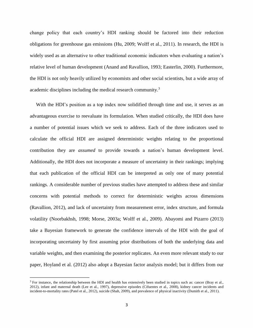
relationship between factor scores for both a country,𝑖, and its neighbors. While neighbors can

be defined in a number of ways, we use the simplest definition based on adjacency in terms of

either a land or maritime connection. We define a set of neighbors for country 𝑖as ℛ𝑖 , and

specify the conditional distribution of the country’s factor score in the following way:

𝛿𝑖|𝛿𝑗~𝑁(∑ 𝜔𝛿𝑗𝑗∈ℛ𝑖

, 𝜈)

where 𝜔 measures degree of spatial correlation and the conditional variance, 𝜈, is a measure of

residual variation.

Primarily, our specification has two attractive properties. First, it intuitively defines the

relationship between neighboring countries through the distribution mean of factor scores. More

flexible models could include additional levels of dependence through both the conditional mean

and conditional variance, but these are not statistically identified within a factor analysis model.8

Second, by setting the conditional variance such that𝜈 = 1, our conditional specification results

in a simple marginal distribution for the vector of factor scores:

𝛿~N(0, (𝐼 − 𝜔𝑊)−1)

where 𝑊 is an 𝑁 × 𝑁 “neighbor matrix” such that 𝑊𝑖𝑘 = 𝑊𝑘𝑖 = 1 if a country 𝑘 is adjacent to

country 𝑖 in terms of either land or maritime connections, and 𝑊𝑖𝑘 = 0 if otherwise.

Additionally, 𝑊𝑖𝑖 = 0. It is also important to note that since the variance matrix of 𝛿 is a full

matrix under this specification, all countries are correlated with one another even if they do not

share a common border.

8 For a more detailed discussion of this, see Hogan and Tchernis (2004).

9

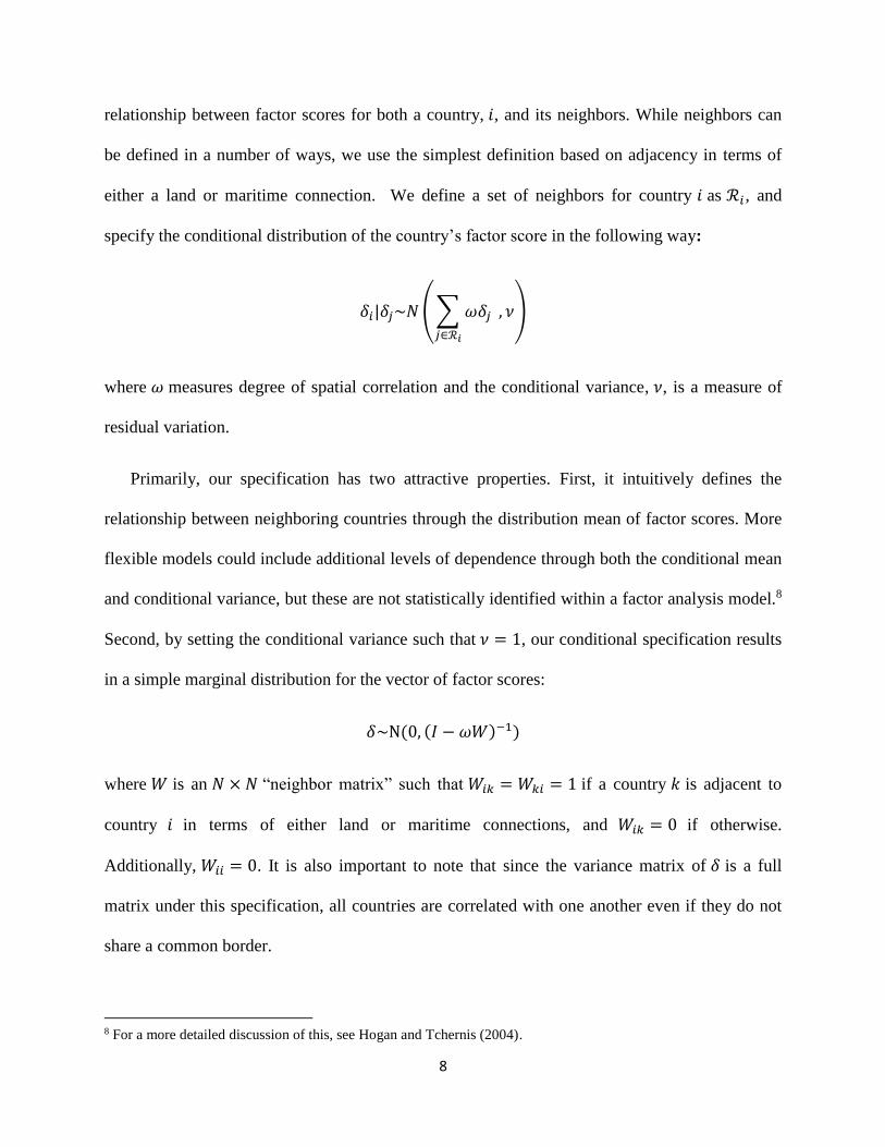
For our last step of model development, we introduce population sizes into both the inverse

variance of the error terms and factor scores. The intuition is that a priori we are less uncertain

regarding the amount of noise in the manifest variables and factor scores of countries with larger

populations compared to countries with smaller populations.

The final model, in vector notation, is now presented as:

𝑌|𝛿~𝑁(𝜇 + 𝛬𝛿,𝑀−1⨂𝛴)

𝛿~N(0,𝑀−12𝝍𝑀−

12)

where 𝑌 is a vector of 𝑌𝑖𝑗’s stacked over j and then i; 𝛬 = 𝐼𝑁⨂𝜆, with 𝐼𝑁 as an 𝑁 × 𝑁 identity

matrix, 𝜆 = (𝜆1, 𝜆2, … , 𝜆𝐽)′𝑎𝑛𝑑⨂ denotes a Kronecker product; 𝛴 is a diagonal matrix with 𝜎𝑗

2

as the diagonal elements, and 0’s as the off-diagonal elements; 𝝍 = (𝐼 − 𝜔𝑊)−1; 𝑀 is an 𝑁 × 𝑁

matrix with country populations 𝑚1, 𝑚2, … ,𝑚𝑁 along the diagonal and 0’s elsewhere.

To complete the model we also specify the prior distribution of our parameters. We use a set

of conjugate, but non-informative, priors which simplify the derivation of the posterior

distributions without providing much information. This implies that the posterior distributions

are informed primarily from the data and not the prior distribution assumptions. We delegate the

details of this to Appendix I.

Following Hogan and Tchernis (2004), we work with the variance stabilizing square root

transformation of the original variables, such that 𝑌𝑖𝑗 = (𝑆𝑖𝑗)1

2, where 𝑆𝑖𝑗’s are the HDI’s non-

10

transformed variables.9 This implies that 𝑣𝑎𝑟(𝑌𝑖𝑗) is inversely proportionate to the country’s

population, 𝑚𝑖 (Cressie and Chan, 1989; Hogan and Tchernis, 2004).

Our model is estimated using Markov Chain Monte Carlo (MCMC) methods, specifically

Metropolis-Hastings with Gibbs Sampler. The method’s primary goal is to produce a summary

of the distribution of ranks for each of country. At each iteration of the sampler, for which we

run 4,000 total iterations after the convergence phase of 500 iterations, we rank the draws from

the posterior distribution of the factor scores. This allows us to produce samples from the

posterior distribution of the countries’ ranks. A more detailed description of the estimation

process can be found in Appendix I.

Our Bayesian methodology can be seen as an improvement over the methodology of official

HDI in several respects. First, our model based ranks are a function of the weighted manifest

variables. This implies that the weights are informed by the data as opposed to expert opinion.

Second, we are able to provide a summary of uncertainty through our ranking distributions.

Third, our rank for each country is informed by data for both the specific country and any

potential spillover effects from neighboring countries using spatial correlation. Finally, we

incorporate additional information contained in a country’s population, resulting in a priori

lower uncertainty for more populous nations. Even though our model provides a flexible

structure for the estimation of country ranks, there are a number of potential sensitivity issues

which we also address in Section 5.

Using the methods outlined in this section, we calculate three sets of ranks: ranks using only

data from the official HDI, ranks for our green HDI which combines official HDI data and an

9 𝑆𝑖𝑗 is already in a “per-capita” form (e.g. GNI per capita, population mean years of schooling, etc.).

11

environmental dimension, and the ranks for our MDG index which uses a comprehensive set of

variables found in the MDG data. The next section explains the sources for our data as well as

information regarding any variable selection.

3. Data

Data for model based HDI

For data pertaining to official HDI variables, we utilize the data used to construct 2010’s official

HDI. The data for each of the 195 countries are publicly available on the UNDP’s website.10 Of

the full dataset we collected, 8 of the 195 countries are excluded from our estimation due to

missing data as they are also removed from the estimation of official HDI. The four manifest

variables used to calculate official HDI are: years of life expectancy at birth, mean years of

schooling for adults, the expected years of schooling for children, and GNI per capita. For our

measure of spatial correlation, we use both land and maritime borders to construct the “neighbor

matrix” W. Country population measures for 2010 are gathered from the World Bank’s total

population midyear estimates.11

Since our model’s ability to add information from new variables without assuming their effect

a priori is perhaps its greatest strength, we exemplify this contribution through our estimation of

a green HDI which includes an environmental variable not found in the official HDI. The

purpose of including an environmental variable is to account for a nation’s environmental

sustainability with respect to their human development factors. We use CO2 emissions per capita

10 The data was downloaded on 06/01/2016 from http://hdr.undp.org/en/data. 11 World Bank Total Population Data: http://data.worldbank.org/indicator/SP.POP.TOTL?page=1

12

(hereafter CO2 ) for the purposes of this paper. One common hurdle prior research has

encountered when adding CO2 to their models is the inherently uncertain relationship between

carbon emissions and development levels.12 Unlike previous studies (Fuentes-Nieva and Pereira,

2010; Bravo, 2014) which rely on assumptions regarding the effect of CO2 on human

development, our method uses only the data to inform the model about this relationship, with the

sign of the factor loading communicating whether CO2 contributes positively to a nation’s

human development level or not. National CO2 emissions per capita data for 2010 are collected

from the 2014 Human Development Report (UNDP and Malik, 2014).

Data for constructing the Millennium Development Goals index

While we show the potential for our model to estimate and add variables to an existing index, our

method also applies to the creation of new and more complex indices as well. We illustrate this

by designing a novel index for measuring human development using the United Nation’s

Millennium Development Goals (MDG). The MDG includes 8 broad primary goals with a total

of 80 indicator variables used to track their progress. Due to the large number of MDG variables

we choose to include in the estimation, our model has an inherent advantage in that we are able

to skip the deterministic assignment of factor weights a priori, as they are a direct product of our

model’s estimation. We can also ignore assumptions regarding variable groupings, allowing us to

avoid a high quantity of extra correlation parameters. Using our model, correlations between

variables, regardless of their dimensions, are captured solely by the spatial correlation structure

embedded in the latent factor.

12 The functional form of our environmental variable is addressed more extensively in Section 5.

13

Data for each MDG variable is collected directly from the United Nation Development

Program.13 While primary target data is available for 234 countries and comparable areas, there

is a considerable quantity of missing observations in the UNDP’s dataset. With this in mind, of

the 80 potential MDG indicator variables available to us we select the 12 which have the most

complete data across countries to serve as our MDG index’s manifest variables.14 Comparing

datasets across time, we also find 2010 to be the year with the most complete collection of data

for the greatest number of countries. To help ensure accurate post-analysis comparisons between

the HDI and our new MDG index, we restrict the selection of observations for our MDG data to

the same 187 countries ranked by the official HDI.

After selecting our manifest variables, we impute values for the missing MDG data using two

separate methods. The first round of imputation is a naïve imputation process for which the

variables are imputed in order from those with the highest to the lowest number of non-missing

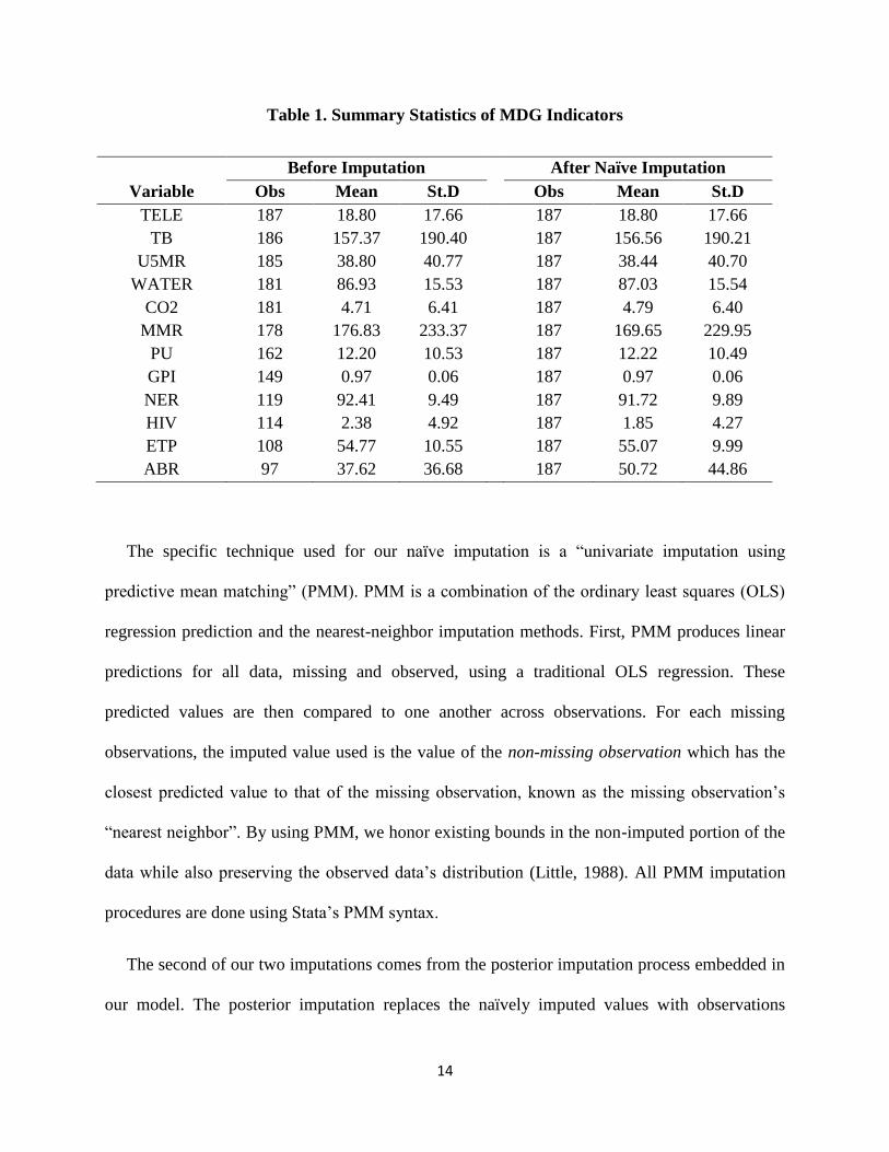
observations. Table 1 presents summary statistics for the 12 manifest variables both before and

after the naïve imputation. As it shows, the number of missing observations among variables

varies considerably, and the change in variable means and standard deviations following the

naïve imputation is relatively low.

13 Millennium Development Goals Indicators: http://mdgs.un.org/unsd/mdg/Data.aspx 14 The 12 selected indicators are: (1) “maternal morality ratio per 100,000 live births” (MMR), (2) “children under

five mortality rate per 1,000 live births” (U5MR), (3) “population undernourished, percentage”(PU), (4) “total net

enrolment ratio in primary education, both sexes”(NER), (5) “gender parity index in primary level enrolment” (GPI),

(6) “tuberculosis prevalence rate per 100,000 population (mid-point)” (TB), (7) “proportion of the population using

improved drinking water sources” (WATER), (8) “people living with HIV, 15-49 years old, percentage” (HIV), (9)

“carbon dioxide emissions (CO2), metric tons of CO2 per capita (CDIAC)” (CO2), (10) “fixed-telephone

subscriptions per 100 inhabitants” (TELE), (11) “employment-to-population ratio, both sexes, percentage” (ETP),

and (12) “adolescent birth rate, per 1,000 women” (ABR).

14

Table 1. Summary Statistics of MDG Indicators

Before Imputation After Naïve Imputation

Variable Obs Mean St.D Obs Mean St.D

TELE 187 18.80 17.66 187 18.80 17.66

TB 186 157.37 190.40 187 156.56 190.21

U5MR 185 38.80 40.77 187 38.44 40.70

WATER 181 86.93 15.53 187 87.03 15.54

CO2 181 4.71 6.41 187 4.79 6.40

MMR 178 176.83 233.37 187 169.65 229.95

PU 162 12.20 10.53 187 12.22 10.49

GPI 149 0.97 0.06 187 0.97 0.06

NER 119 92.41 9.49 187 91.72 9.89

HIV 114 2.38 4.92 187 1.85 4.27

ETP 108 54.77 10.55 187 55.07 9.99

ABR 97 37.62 36.68 187 50.72 44.86

The specific technique used for our naïve imputation is a “univariate imputation using

predictive mean matching” (PMM). PMM is a combination of the ordinary least squares (OLS)

regression prediction and the nearest-neighbor imputation methods. First, PMM produces linear

predictions for all data, missing and observed, using a traditional OLS regression. These

predicted values are then compared to one another across observations. For each missing

observations, the imputed value used is the value of the non-missing observation which has the

closest predicted value to that of the missing observation, known as the missing observation’s

“nearest neighbor”. By using PMM, we honor existing bounds in the non-imputed portion of the

data while also preserving the observed data’s distribution (Little, 1988). All PMM imputation

procedures are done using Stata’s PMM syntax.

The second of our two imputations comes from the posterior imputation process embedded in

our model. The posterior imputation replaces the naïvely imputed values with observations

15

sampled from the distributions of missing data. This allows us to take potential uncertainty

inherent in the missing data into better account (Rubin, 1976; Little and Rubin, 2002; Daniels

and Hogan, 2008). We address the posterior imputation more fully, along with the sensitivity of

our results to the choice of imputation process, in Section 5.

4. Results

Model based ranks vs. official HDI ranks

The rankings of official HDI fail to account for either uncertainty, spatial correlation, or

population. Alternatively, our index ranks are estimated in terms of distributions, which provide

a measure of uncertainty. Since factor weightings are different between our model-based index

and the official HDI, there must be some differences between the posterior mean ranks and the

official HDI ranks. We compare the two rankings, including the information for the 99%

confidence interval of the posterior ranks, in Figure 1.

For Figure 1 and subsequent figures of the same layout, the dashed grid lines partition the

0%-20% (1st), 20%-40% (2nd), 40%-60% (3rd), 60%-80% (4th), and 80%-100% (5th) quintiles of

ranks respectively. The solid dots show the locations of both posterior mean ranks and official

HDI ranks. Solid horizontal lines across each dot represent the 99% confidence interval for each

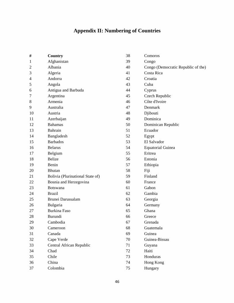
country’s posterior model based rank. The numbers in Figure 1 correspond to individual country

identifiers, which are assigned alphabetically and can be referenced in Appendix II.

16

It is immediately apparent that our model’s rankings harbor a considerable level of

uncertainty for some countries, with several confidence intervals even reaching across quintiles.

Interestingly, this uncertainty persists in various degrees along the entire spectrum of ranks as

opposed to being prevalent in only certain categories of development. As an example, Bhutan, a

low development level country, has a posterior 99% confidence interval of (141, 164), implying

that their rank could fall into either the 4th or the 5th quintile. Similar results are also found for

more highly developed nations like Kuwait, which has a posterior 99% confidence interval of

(10, 45), implying that its rank could fall into either the 1st or 2nd quintiles. While Bhutan and

Kuwait represent the most extreme examples, it is not uncommon for nations to be categorized

into different quintiles given their confidence intervals.

The relationship between the rank of the country and the amount of uncertainty is an inverted

U-shape, with levels of uncertainty decreasing for the most and least developed countries. This is

due to a number of factors. First, countries ranked and the top (bottom) have the highest (lowest)

values for each manifest variable. Second, these often tend to be the most populous countries.

Third, they are also closer to one another on average geographically, leading to a reduction in

uncertainty through spatial smoothing. Finally, this is also due to the truncation of variable

values from both below or above for the most and least developed countries.

Another feature of Figure 1 is that it shows the discordance between our model-based ranks

and those of the official HDI. The greater the distance between solid dots and the 45o line, the

greater the disagreement between our model-based ranks and the ranks of official HDI. For only

9 countries are our model-based and official HDI ranks the same. For 87 countries, the absolute

value of difference between the two ranks is less than 5. For 54 countries however, the absolute

value of difference is larger than 10.

17

Figure 1. Posterior Mean and 99% CI of Model-based HDI Ranks vs. Official HDI Ranks

Discordance between model based and official HDI ranks

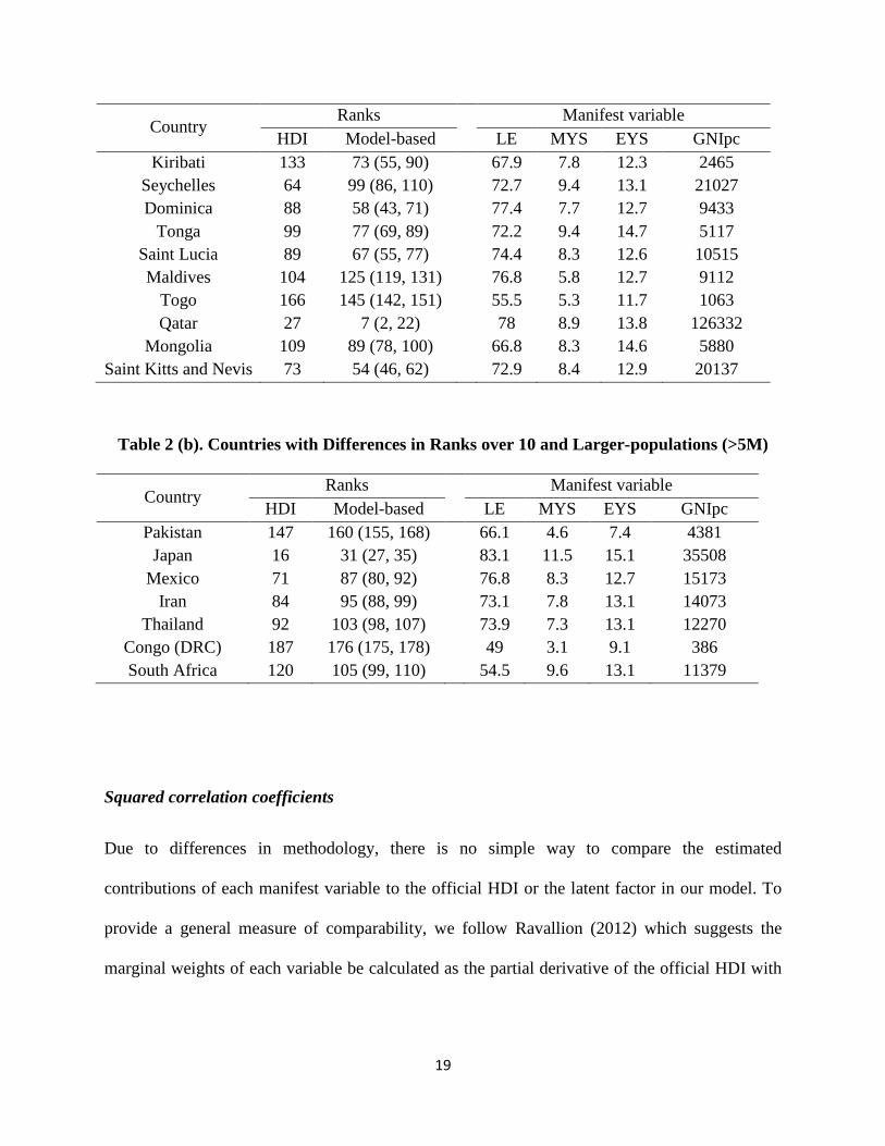
Table 2(a) shows the ten countries which have the largest differences between their official HDI

rankings and their rankings as determined by our model. As an example, Mongolia is ranked 109

in the 2010 official HDI; but is assigned a posterior mean rank of 89 by our model with a 99%

confidence interval of (78, 100). Therefore, Mongolia’s posterior confidence interval fails to

even cover the range of its official HDI rank. It is reasonable to conclude from our results that

18

the official HDI underestimates Mongolia’s level of human development. Alternatively, Mexico,

which has an official HDI rank of 71, has posterior mean rank of 87 in our model with a 99%

confidence interval of (80, 92). So, in an opposite pattern to Mongolia, the official HDI seems to

very much overestimate the human development level of Mexico given our findings. Since the

majority of these highly discordant countries have relatively small populations, we also present

the seven nations with large populations (over five million) which also have a difference-in-

ranks between their model based and official HDI rankings larger than 10 in Table 2(b).

The most plausible reason behind these large discordances in rank is the difference in factor

weights between the official HDI and our model based index. As we discuss in the following

section, our model based index assigns a greater proportional contribution to the “living standard”

indicator but a lower proportional contribution to the “longevity” indicator; implying that

countries with either outstanding or dismal performance in these two dimensions see a

considerable amount of movement between the two indices.

Table 2 (a). Ten Countries with the Largest Differences in Ranks

Between Official HDI and Model-based HDI

19

Country Ranks Manifest variable

HDI Model-based LE MYS EYS GNIpc

Kiribati 133 73 (55, 90) 67.9 7.8 12.3 2465

Seychelles 64 99 (86, 110) 72.7 9.4 13.1 21027

Dominica 88 58 (43, 71) 77.4 7.7 12.7 9433

Tonga 99 77 (69, 89) 72.2 9.4 14.7 5117

Saint Lucia 89 67 (55, 77) 74.4 8.3 12.6 10515

Maldives 104 125 (119, 131) 76.8 5.8 12.7 9112

Togo 166 145 (142, 151) 55.5 5.3 11.7 1063

Qatar 27 7 (2, 22) 78 8.9 13.8 126332

Mongolia 109 89 (78, 100) 66.8 8.3 14.6 5880

Saint Kitts and Nevis 73 54 (46, 62) 72.9 8.4 12.9 20137

Table 2 (b). Countries with Differences in Ranks over 10 and Larger-populations (>5M)

Country Ranks Manifest variable

HDI Model-based LE MYS EYS GNIpc

Pakistan 147 160 (155, 168) 66.1 4.6 7.4 4381

Japan 16 31 (27, 35) 83.1 11.5 15.1 35508

Mexico 71 87 (80, 92) 76.8 8.3 12.7 15173

Iran 84 95 (88, 99) 73.1 7.8 13.1 14073

Thailand 92 103 (98, 107) 73.9 7.3 13.1 12270

Congo (DRC) 187 176 (175, 178) 49 3.1 9.1 386

South Africa 120 105 (99, 110) 54.5 9.6 13.1 11379

Squared correlation coefficients

Due to differences in methodology, there is no simple way to compare the estimated

contributions of each manifest variable to the official HDI or the latent factor in our model. To

provide a general measure of comparability, we follow Ravallion (2012) which suggests the

marginal weights of each variable be calculated as the partial derivative of the official HDI with

20

respect to each variable.15 Following this, we can therefore obtain the marginal weights of each

variable in the official HDI by regressing standardized HDI scores on standardized manifest

variables.

To summarize the contribution of each variable to the latent factor in our model, we apply the

methods of Hogan and Tchernis (2004) and present normalized “squared correlation

coefficients”. The “squared correlation coefficient” for each variable 𝑗 is specified as:

ρj2 =

λj2

λj2 + 𝜎𝑗

2

Each correlation coefficient is the proportion of variation in the manifest variable, 𝑗, that is

explained by the latent human development factor. In Table 3, we compare the normalized

marginal weights for each manifest variable of the official HDI to the normalized “squared

correlation coefficients” produced by our model-based index.

Table 3. Comparison of HDI Weights and Normalized Squared Correlations 𝛒𝟐

Variable HDI Weights (95% CI) ρ2(95% CI)

Life Expectancy at Birth 0.33 (0.32, 0.34) 0.19 (0.17, 0.20)

Mean Years of Schooling 0.29 (0.29, 0.29) 0.27 (0.27, 0.28)

Expected Years of Schooling 0.23 (0.22, 0.24) 0.27 (0.27, 0.28)

GNI per capita 0.15 (0.14, 0.15) 0.26 (0.26, 0.27)

15 For a more detailed overview, see Ravallion (2012).

21

With respect to our results, we find the “longevity” dimension offers a lower contribution to a

country’s human development level than the weights of official HDI would suggest. Our model

also attributes a much greater contribution to the “living standard” dimension when compared to

official HDI. Additionally, while the official HDI assigns a greater proportional contribution to

“mean years of schooling” than “expected years of schooling”, our model assigns identical levels

of contribution to both variables of the “education” dimension.

The most and least developed countries

One of the HDI’s primary purposes is to identify the countries with both the highest and lowest

levels of human development. Distinguishing countries with best practices establishes role

models for other nations; while identifying the least developed countries has significant

implications for nations with lower levels of human development. Since comparing the relative

performance of nations is so important, it again becomes a potential concern that the official HDI

offers only a single rank for each country as opposed to a plausible range of values. This can be

especially detrimental to countries which border the poorest rankings of human development, as

it may disqualify them from participating in beneficial international assistance programs should

their official HDI rank fall outside of a program’s bounds. Since our method produces

distributions of ranks, we are able to estimate and assign probabilities for each country to be

among the least or most developed.

In Figure 2 we estimate the probability of countries being among the top 10 most developed

countries using our model, along with their official HDI rankings. Of the 187 total countries, 17

have non-zero probabilities of being included in our model’s “Top 10”. Additionally, for these

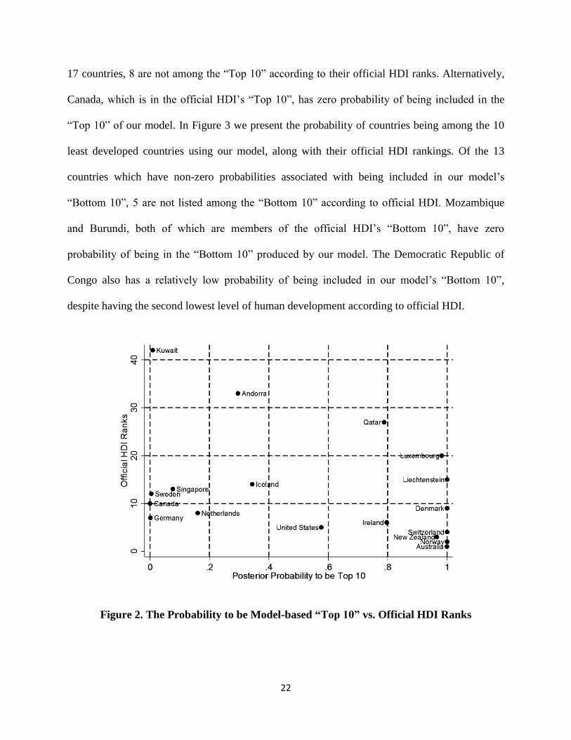
22

17 countries, 8 are not among the “Top 10” according to their official HDI ranks. Alternatively,

Canada, which is in the official HDI’s “Top 10”, has zero probability of being included in the

“Top 10” of our model. In Figure 3 we present the probability of countries being among the 10

least developed countries using our model, along with their official HDI rankings. Of the 13

countries which have non-zero probabilities associated with being included in our model’s

“Bottom 10”, 5 are not listed among the “Bottom 10” according to official HDI. Mozambique

and Burundi, both of which are members of the official HDI’s “Bottom 10”, have zero

probability of being in the “Bottom 10” produced by our model. The Democratic Republic of

Congo also has a relatively low probability of being included in our model’s “Bottom 10”,

despite having the second lowest level of human development according to official HDI.

Figure 2. The Probability to be Model-based “Top 10” vs. Official HDI Ranks

23

Figure 3. The Probability to be Model-based “Bottom 10” vs. Official HDI Ranks

Incorporation of an environmental indicator

We incorporate CO2 to construct a model of HDI with an additional indicator representing a

country’s environmental stewardship and emissions level. We present the posterior ranks of our

green HDI with those of the 2010 official HDI in Figure 4. The inclusion of CO2 shifts the

posterior ranks of some countries and presents slightly more discordance between the ranks of

our model and the ranks of official HDI compared to the results of our model withoutCO2.

Without CO2 the sum of absolute differences between the ranks of our model and those of the

official HDI is 1335.9. After includingCO2, the sum of absolute differences increases to 1463.9,

implying a 10% increase in discordance between our model’s results and the ranks of official

24

HDI when using CO2 .16 Comparing the results of our model with and without CO2 to one

another, we find the sum of absolute differences to be 1038.99.17 This implies that while there is

a level of disagreement between the ranks of our model under different specifications, it is lower

than the level of discordance for either model when compared to the official HDI.

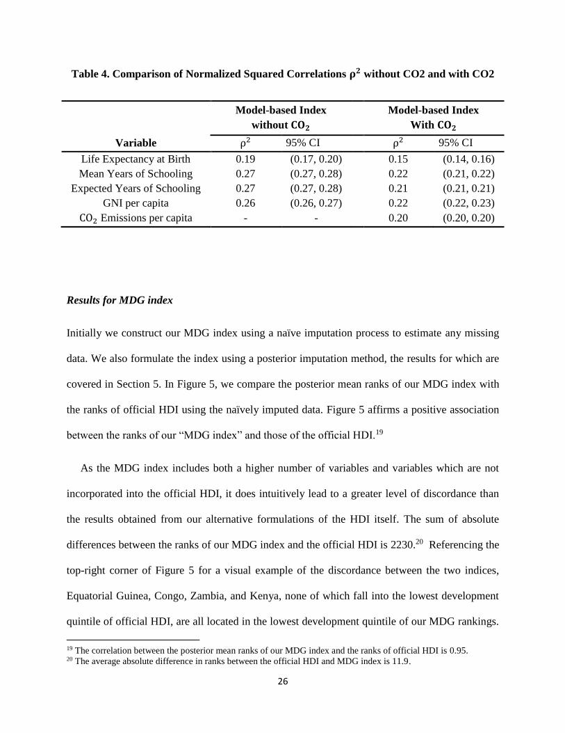
Table 4 shows the specific changes in the “squared correlation coefficients” between the

rankings of our model with and without CO2. While “education” remains the dominant indicator

of human development, the proportional contribution attributed to CO2 is similar to that of the

other variables. The contribution of “health” also becomes smaller after adding the

environmental dimension, which is likely a result of CO2 capturing certain health issues

associated with a country’s pollution level. The addition of CO2 also leads to considerable

movements in rank for several oil producing nations. As example, Trinidad and Tobago and

Kuwait, which are ranked 63 and 42 respectively by official HDI, both see dramatic

improvements in rank under our green HDI model; moving to posterior mean rankings of 30.69

and 4.86 respectively.

Another interesting difference between the rankings of our model with and without CO2 is

that the ranks of our green HDI are estimated with less uncertainty than the ranks of our original

model. This can be seen by comparing the confidence intervals shown in Figure 4 to those of

Figure 1. To confirm this, we also sum the standard deviations of the posterior ranks for each

country produced by our model with and without CO2. After including CO2, the sum of standard

deviations of our posterior ranks decreases from 397.9 to 352.9, an 11% decline, indicating less

16 The average absolute difference in ranks between the official HDI and our model increases from 7.1 to 7.8 after

including CO2. 17 The average absolute difference in ranks between our model with and without CO2 is 5.6.

25

uncertainty.18 One possible reason for this is that we simply accept the positive correlation

between CO2 and the official HDI score. Since we let the factor loading produced by our model

decide the direction of its contribution to human development, CO2 is incorporated “as is”

without alteration to its direction or functional form. The sensitivity of our model to functional

form changes of CO2 is explored in Section 5.

Figure 4. Posterior Mean and 99% CI of Model-based “Green” HDI Ranks

vs. Official HDI Ranks

18 The average standard deviation in posterior country rank decreases from 2.13 to 1.89.

26

Table 4. Comparison of Normalized Squared Correlations 𝛒𝟐 without CO2 and with CO2

Model-based Index

without 𝐂𝐎𝟐

Model-based Index

With 𝐂𝐎𝟐

Variable ρ2 95% CI ρ2 95% CI

Life Expectancy at Birth 0.19 (0.17, 0.20) 0.15 (0.14, 0.16)

Mean Years of Schooling 0.27 (0.27, 0.28) 0.22 (0.21, 0.22)

Expected Years of Schooling 0.27 (0.27, 0.28) 0.21 (0.21, 0.21)

GNI per capita 0.26 (0.26, 0.27) 0.22 (0.22, 0.23)

CO2 Emissions per capita - - 0.20 (0.20, 0.20)

Results for MDG index

Initially we construct our MDG index using a naïve imputation process to estimate any missing

data. We also formulate the index using a posterior imputation method, the results for which are

covered in Section 5. In Figure 5, we compare the posterior mean ranks of our MDG index with

the ranks of official HDI using the naïvely imputed data. Figure 5 affirms a positive association

between the ranks of our “MDG index” and those of the official HDI.19

As the MDG index includes both a higher number of variables and variables which are not

incorporated into the official HDI, it does intuitively lead to a greater level of discordance than

the results obtained from our alternative formulations of the HDI itself. The sum of absolute

differences between the ranks of our MDG index and the official HDI is 2230.20 Referencing the

top-right corner of Figure 5 for a visual example of the discordance between the two indices,

Equatorial Guinea, Congo, Zambia, and Kenya, none of which fall into the lowest development

quintile of official HDI, are all located in the lowest development quintile of our MDG rankings.

19 The correlation between the posterior mean ranks of our MDG index and the ranks of official HDI is 0.95. 20 The average absolute difference in ranks between the official HDI and MDG index is 11.9.

27

Therefore, the official HDI is likely overestimating the development levels of these countries

with respect to the findings of our MDG index. Alternatively, with reference to the bottom-left

corner of Figure 5, Brunei and Lithuania are both ranked outside of the most developed quintile

of our posterior MDG ranks while they are included in the most developed quintile of the official

HDI. It is therefore possible that the official HDI overestimates the development level of these

countries given our findings. We also find the total level of uncertainty produced by our MDG

index to be lower than our estimations of HDI and green HDI, with a sum standard deviations of

264, corresponding to an average standard deviation in ranks of 1.4.

28

Figure 5. Posterior Mean and 99% CI of Model-based MDG Ranks vs. Official HDI Ranks

5. Sensitivity Analysis

In this section we explore the sensitivity of our results with regards to three aspects of the data.

First, we address the sensitivity to choices of functional form by comparing results using GNIpc

vs. ln(GNIpc), which is used in calculating the official HDI. Second, we compare the results

29

using CO2 vs. ln(CO2). Finally, we address the sensitivity to the choice of methods used to

impute the missing data of our MDG index.

Calculating HDI using the logarithm of GNI per capita

To account for the diminishing effect of income on development, we use the natural logarithm of

GNI per capita as an alternative measure in our model based HDI. Recall that the official HDI

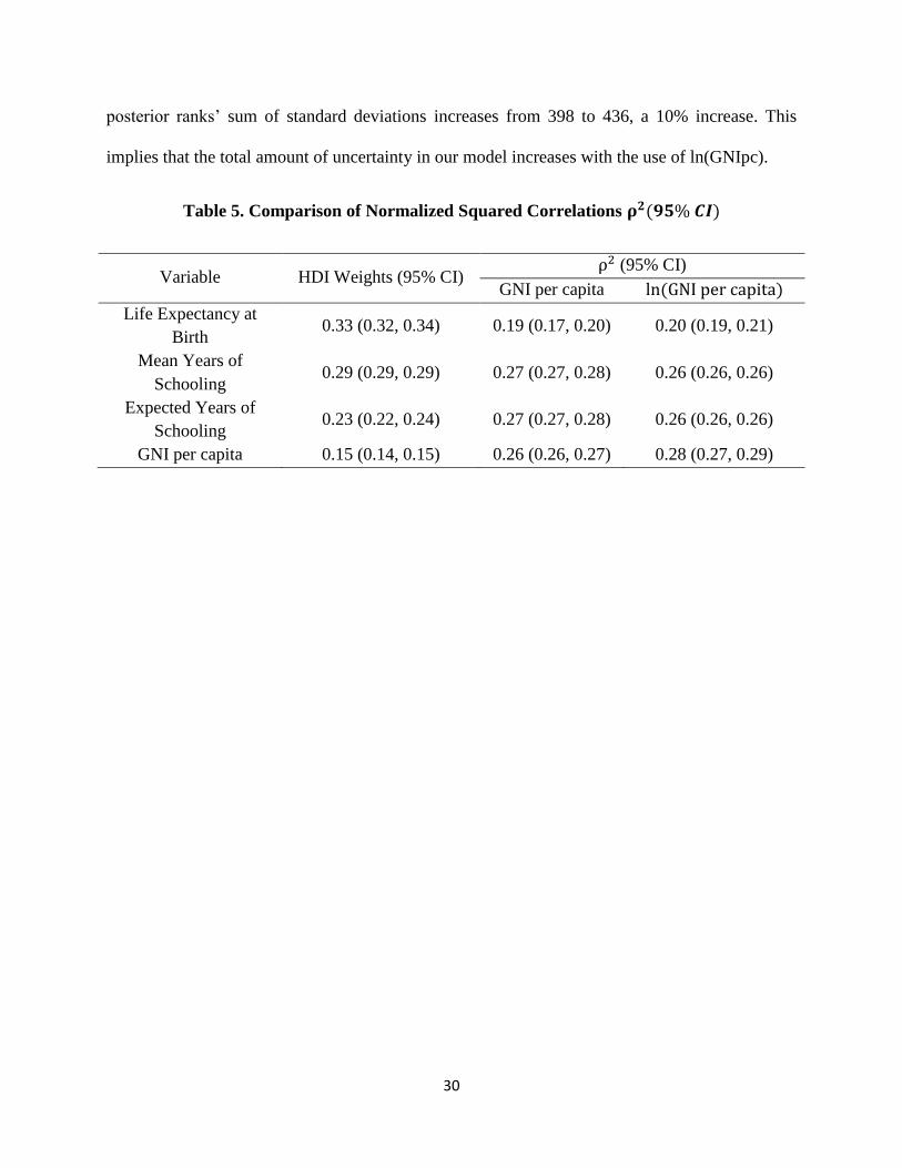
also uses the logarithm of GNIpc to calculate their Income Index. Table 5 compares the

normalized “squared correlation coefficients” of our model using both GNI per capita and

ln(GNIpc), along with the factor weightings of official HDI. We can see that there are no

substantial changes in the squared correlation coefficient due to the change in the functional form

of GNIpc.

Figure 6 presents our model based ranks using ln(GNIpc) versus the ranks of official HDI.

Looking between Figure 6 and Figure 1, we see that changing the functional form of GNI per

capita does not substantially alter the posterior ranks of our model. However, comparing the

ranks of our model and the official HDI, the sum of absolute differences between the official

HDI and our model based index using ln(GNIpc) decreases from 1337 to 986, a decline of

26%.21 This is most likely due to the fact that ln(GNIpc) is the functional form specification used

to calculate the official HDI’s Income Index. The discordance between the results of our model

using GNI per capita and ln(GNIpc) is 640, which is 35% smaller than the discordance between

the ranks of official HDI and our model-based index using ln(GNIpc).22 While the discordance

between the results of our model and the official HDI decreases when using ln(GNIpc), the

21 The average absolute difference in rank between official HDI and our model is 5.8 when using ln(GNI),

comparing to 7.1 when using GNI per capita. 22 The average absolute difference in rank between our model with GNI per capita and ln(GNI) is 3.4.

30

posterior ranks’ sum of standard deviations increases from 398 to 436, a 10% increase. This

implies that the total amount of uncertainty in our model increases with the use of ln(GNIpc).

Table 5. Comparison of Normalized Squared Correlations 𝛒𝟐(𝟗𝟓%𝑪𝑰)

Variable HDI Weights (95% CI) ρ2 (95% CI)

GNI per capita ln(GNIpercapita)

Life Expectancy at

Birth 0.33 (0.32, 0.34) 0.19 (0.17, 0.20) 0.20 (0.19, 0.21)

Mean Years of

Schooling 0.29 (0.29, 0.29) 0.27 (0.27, 0.28) 0.26 (0.26, 0.26)

Expected Years of

Schooling 0.23 (0.22, 0.24) 0.27 (0.27, 0.28) 0.26 (0.26, 0.26)

GNI per capita 0.15 (0.14, 0.15) 0.26 (0.26, 0.27) 0.28 (0.27, 0.29)

31

Figure 6. Posterior Mean and 99% CI of Model-based Ranks vs. Official HDI Ranks

Using ln(GNI per capita)

Calculating green HDI with the logarithm of 𝑪𝑶𝟐

We observe a positive association between CO2 level and country specific human development

level, as measured by official HDI score. Figure 7(a) shows the relationship between official

HDI score and CO2 in 2010 for the 187 countries of our sample. Figure 7(b) shows the same

32

relationship, except delineated by the official HDI’s development level categories. 23 For

countries in the categories of “low development”, “medium development” and “high

development”, the relationship between CO2 and official HDI ranking is apparently positive. It is

only for countries in the “very high development” category that the association become

seemingly insignificant.24

While the relationship between CO2 and human development level is positive, it is decidedly

non-linear. To account for this, we also formulate our green HDI ranks using the natural

logarithm of CO2. Table 6 compares the normalized “squared correlation coefficients” using each

possible functional form combination of both GNI per capita and CO2. The small variation in

variable contributions between estimations further substantiates our claim that the logarithmic

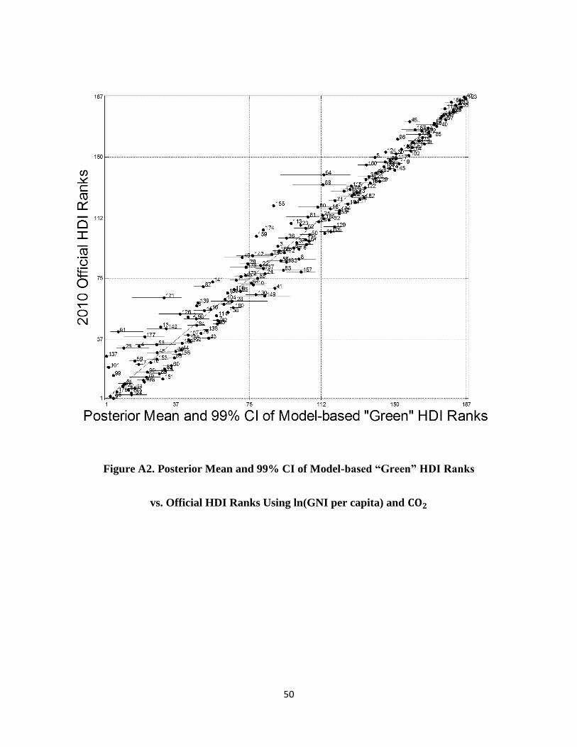
functional form does little to alter the factor weightings of our model-based index. Figures A1,

A2 and A3 in Appendix III display the ranks of our green HDI versus those of the official HDI

using the specifications in columns (2), (3), and (4) of Table 6. When compared to Figure 6,

alteration to the functional form of CO2 seems to have a negligible effect on the level of

discordance between our green HDI and official HDI for each of the three estimations.

As discussed in the previous section, using the logarithm of GNI per capita results in a

considerable decrease in discordance between the ranks of our model and the official HDI. Using

the logarithm of GNI per capita in our green HDI also decreases the level of discordance

between our model and the official HDI, resulting in a decrease in the sum of absolute

differences in rank from 1464 to 1334, a decline of 9%.25 The sum of absolute differences

23 “very high development” (HDI≥0.8), “high development” (HDI 0.7-0.8), “medium development” (HDI 0.55-0.7),

and “low development” (HDI<0.55) 24 The correlation coefficients between CO2 emissions and official HDI are 0.50, 0.31, 0.37, and -0.06 for countries

of “low development”, “medium development”, “high development” and “very high development”, respectively. 25 The average of absolute differences in rank decreases from 7.8 to 7.1.

33

between our green HDI ranks with GNI per capita and ln(GNI) is 572, corresponding to an

average difference of 3.1. Using ln(GNI) in our green HDI also leads to an increase in

uncertainty compared to our green HDI index with GNI per capita. The sum of standard

deviations changes from 353 to 385 when using ln(GNI), an increase of 9%.26

We also see that using the logarithm of CO2 substantially decreases the discordance between

the ranks of our model and the official HDI, leading to a decrease in the sum of absolute

differences in ranks from 1464 to 1255, a decline of 14%.27 Comparing the results of our model

with and without the logarithm of CO2, the sum of absolute differences between the two indices

is 462, corresponding to an average difference in rank of 2.5. Additionally, the total amount of

uncertainty changes very little for our model when using different functional forms of CO2.28

Tables showing the measures of discordance and uncertainty between all functional form

combinations produced by our model are shown in Appendix IV.

26 The average standard deviation increases from 1.9 to 2.1. 27 The average of absolute differences in rank decreases from 7.8 to 6.7. 28 Compared to using CO2, the inclusion of the logarithm of CO2 leads to only a 1% increase in total uncertainty.

34

(a)

(b)

Figure 7. Relationship between 𝑪𝑶𝟐 and Official HDI for Countries with Different HDI

Score in 2010

35

Table 6. Comparison of Normalized Squared Correlations 𝛒𝟐(𝟗𝟓%𝑪𝑰)

GNI per capita ln(GNIpercapita)

(1) (2) (3) (4)

Variable CO2 ln(CO2) CO2 ln(CO2)

Life Expectancy at Birth 0.15 (0.14, 0.16) 0.16 (0.15, 0.17) 0.16 (0.15, 0.17) 0.16 (0.15, 0.17)

Mean Years of Schooling 0.22 (0.21, 0.22) 0.22 (0.21, 0.23) 0.21 (0.21, 0.21) 0.20 (0.20, 0.20)

Expected Years of Schooling 0.21 (0.21, 0.21) 0.22 (0.21, 0.22) 0.20 (0.20, 0.20) 0.20 (0.20, 0.20)

GNI per capita 0.22 (0.22, 0.23) 0.21 (0.21, 0.22) 0.23 (0.23, 0.24) 0.24 (0.23, 0.25)

CO2 Emissions per capita 0.20 (0.20, 0.20) 0.19 (0.19, 0.20) 0.20 (0.19, 0.20) 0.21 (0.20, 0.21)

Results using posterior imputation

Following the naïve imputation process for the MDG dataset, we next formulate our MDG index

using the posterior imputation process built into our model. Figure 8 presents the relationship

between the rankings of our MDG index following posterior imputation and the rankings of

official HDI. We have shown earlier that there is a substantial amount of data missing from

MDG data which were imputed. However, we used these imputed values as data without directly

accounting for the uncertainty of imputation. In this section we incorporate the imputation of

missing data into the estimation algorithm. Similarly to multiple imputations method, the

posterior imputation process also obtains draws from the posterior distribution of the missing

values at each iteration of the sampler. We present the results in Figure 8.

While the posterior mean ranks for most countries remains stable, the uncertainty of rankings

following posterior imputation appears much larger for some countries when compared to the

uncertainty of the naïve imputation results. The more missing values a country has, the more

36

uncertainty it will show following posterior imputation. This leads to countries like Liechtenstein

and Hong Kong having extreme confidence intervals compared to the average. Additionally,

higher levels of missing data increase the magnitude of separation between a country’s naïve and

posterior imputation mean ranks.

Formally measuring the amount of discordance between our model under the two imputation

processes and the official HDI, we see an increase in the sum of squared differences in rank from

42,812 to 55,533 using posterior imputation, a change of almost 30%. While the sum of squared

differences increases considerably following posterior imputation, the sum of absolute

differences remains relatively unchanged (a 4% increase from 2230 to 2322).29 This implies that

several outlier countries see a considerable change in rank between the two imputation methods

while the general discordance changes a comparably small amount. As for the uncertainty, the

sum of standard deviations increases from 264 to 569. Tables showing measures of discordance

and uncertainty for the MDG index under both imputation measures can be found in Appendix

IV.

29 The average of absolute differences in rank increases from 11.9 to 12.4.

37

Figure 8. Posterior Mean and 99% CI of MDG Ranks Using Posterior Imputation

vs. Official HDI Ranks

38

6. Conclusion

In this paper, we propose a Bayesian factor analysis model with the purpose of serving as an

alternate approach to calculating the UNDP’s Human Development Index, as well as providing a

general methodology which can be used to augment existing indices or build new ones. We

address several potential issues of the official HDI using the following methods. First, our model

produces data-driven weights for each manifest variable’s contribution to the latent factor of

human development. This is in contrast to the ad hoc factor weights currently used to calculate

the scores of official HDI. Second, our model reports its posterior ranks in terms of distributions,

incorporating a measure of uncertainty which is absent from the official HDI’s international

rankings. Third, we adjust the level of uncertainty by incorporating a measure of spatial

correlation between countries while also including country populations in our estimation. Each

of these additions helps to improve the precision of our ranking distributions. To then illustrate

the potential applications and flexibly of our model, we estimate an alternative green HDI index

by adding a new environmental variable, CO2. Then as an example of constructing a new index

with a more complex variable structure, we build a novel MDG index using data from the

Millennium Development Goals project.

Under our methodology, we find the “living standard” dimension provides a greater

proportional contribution to human development than it is assigned by the official HDI while the

“longevity” dimension provides a lower proportional contribution. The results of our model also

show considerable levels of general disagreement when compared to the ranks of the official

HDI. Countries which are officially categorized into a particular quintile can even arguably be

assigned to a different quintile under our estimation. Therefore, the nations constituting a

country’s “peers” under the rankings of our model can vary widely from the peers observed

39

under the official HDI, leading to a much different picture of a country’s relative development

level. We also find our incorporation of CO2 to shift the posterior ranks of some countries

substantially, again moving them across quintiles in some cases. It can then be argued that

incorporating CO2 is necessary, as it makes a non-negligible difference in the evaluation of

human development level. Additionally, even with the complicated structure of the MDG’s

indicator variables, we show that our model is able to successfully construct the desired MDG

index. Constructing an MDG index exemplifies the adaptive nature of our methodology and

provides a blueprint which further researchers can implement to efficiently build indices that

may have previously seemed too complex.

Looking to the change in results between different functional forms, we find our model to be

more sensitive to functional alterations of GNI per capita than CO2. The most plausible reason

why changing between GNI per capita and its logarithm causes more variation in estimation is

because the scale of GNI per capita is much larger than that of CO2. This implies the values of

the variable itself change much more between the two specifications. With this said, the amount

of discordance between our model with GNI per capita and the logarithm of GNI per capita is

smaller than the level of discordance between either model specification and official HDI. Also,

after adding CO2 our results become much less sensitive to the same functional form changes of

GNI per capita. We therefore fail to conclude that our methodology is particularly sensitive to

functional form changes. Nonetheless, our model does still allow for the construction of indices

and addition of new variables using the minimum number of assumptions, since none are needed

for either variable grouping or the direction of relationships between the variables used in the

index and the latent factor of interest.

40

References

Abayomi, K. and G. Pizarro (2013). "Monitoring human development goals: A straightforward

(Bayesian) methodology for cross-national indices." Social Indicators Research 110(2): 489-515.

Alkire, S. and M. E. Santos (2010). "Acute multidimensional poverty: A new index for

developing countries." United Nations Development Programme Human Development Report

Office Background Paper (2010/11).

Anand, S. and M. Ravallion (1993). "Human development in poor countries: on the role of

private incomes and public services." The Journal of Economic Perspectives 7(1): 133-150.

Bravo, G. (2014). "The Human Sustainable Development Index: New calculations and a first

critical analysis." Ecological Indicators 37: 145-150.

Bray, F., A. Jemal, N. Grey, J. Ferlay and D. Forman (2012). "Global cancer transitions

according to the Human Development Index (2008–2030): a population-based study." The

Lancet Oncology 13(8): 790-801.

Cifuentes, M., G. Sembajwe, S. Tak, R. Gore, D. Kriebel and L. Punnett (2008). "The

association of major depressive episodes with income inequality and the human development

index." Social Science & Medicine 67(4): 529-539.

Conley, T. G. and E. Ligon (2002). "Economic distance and cross-country spillovers." Journal of

Economic Growth 7(2): 157-187.

Courtemanche, C., S. Soneji and R. Tchernis (2015). "Modeling Area‐Level Health Rankings."

Health Services Research 50(5): 1413-1431.

Cressie, N. and N. H. Chan (1989). "Spatial modeling of regional variables." Journal of the

American Statistical Association 84(406): 393-401.

Daniels, M. J. and J. W. Hogan (2008). Missing data in longitudinal studies: Strategies for

Bayesian modeling and sensitivity analysis, CRC Press.

De Muro, P., M. Mazziotta and A. Pareto (2011). "Composite indices of development and

poverty: An application to MDGs." Social Indicators Research 104(1): 1-18.

Dumith, S. C., P. C. Hallal, R. S. Reis and H. W. Kohl (2011). "Worldwide prevalence of

physical inactivity and its association with human development index in 76 countries."

Preventive Medicine 53(1): 24-28.

Easterlin, R. A. (2000). "The worldwide standard of living since 1800." The Journal of

Economic Perspectives 14(1): 7-26.

Eberhardt, M., C. Helmers and H. Strauss (2013). "Do spillovers matter when estimating private

returns to R&D?" Review of Economics and Statistics 95(2): 436-448.

Ertur, C. and W. Koch (2011). "A contribution to the theory and empirics of Schumpeterian

growth with worldwide interactions." Journal of Economic Growth 16(3): 215-255.

Fattah, S. and A. Muji. (2012). "Local government expenditure allocation toward Human

Development Index at Jeneponto regency, South Sulawesi, Indonesia." International

41

Organization of Scientific Research (IOSR) Journal of Humanities and Social Science 5(6): 40-

50.

Fuentes-Nieva, R. and I. Pereira (2010). "The disconnect between indicators of sustainability and

human development." Human Development Research Paper 34.

Hogan, J. W. and R. Tchernis (2004). "Bayesian factor analysis for spatially correlated data, with

application to summarizing area-level material deprivation from census data." Journal of the

American Statistical Association 99(466): 314-324.

Høyland, B., K. Moene and F. Willumsen (2012). "The tyranny of international index rankings."

Journal of Development Economics 97(1): 1-14.

Hu, A. (2009). "A new approach at Copenhagen." China Dialogue [Accessed on June 1st 2016]:

https://www.chinadialogue.net/article/show/single/en/2892-A-new-approach-at-Copenhagen-1-

Keller, W. (2002). “Geographic localization of international technology diffusion”. The

American Economic Review 92(1): 120-142.

Lee, K., S. Park, B. Khoshnood, H. L. Hsieh and R. Mittendorf (1997). "Human development

index as a predictor of infant and maternal mortality rates." The Journal of Pediatrics 131(3):

430-433.

Little R. J. and D. B. Rubin (2002). "Statistical analysis with missing data." Second Edition.

Wiley Series in Probability and Stistics. New York, NY: Wiley, 2002 1.

Little, R. J. (1988). "Missing-data adjustments in large surveys." Journal of Business &

Economic Statistics 6(3): 287-296.

Malczewski, J. (2010). "Exploring spatial autocorrelation of life expectancy in Poland with

global and local statistics." GeoJournal 75 (1): 79-92.

Morse, S. (2003a). "For better or for worse, till the human development index do us part?"

Ecological Economics 45(2): 281-296.

Morse, S. (2003b). "Greening the United Nations' human development index?" Sustainable

Development 11(4): 183-198.

Neumayer, E. (2001). "The human development index and sustainability—a constructive

proposal." Ecological Economics 39(1): 101-114.

Noorbakhsh, F. (1998). "A modified human development index." World Development 26(3):

517-528.

O'Neill, H. (2005). "Ireland's foreign aid in 2004." Irish Studies in International Affairs 16: 279-

316.

Patel, A. R., S. M. Prasad, Y.-C. T. Shih and S. E. Eggener (2012). "The association of the

human development index with global kidney cancer incidence and mortality." The Journal of

Urology 187(6): 1978-1983.

Petersen, M. and L. Rother (2001). "Maker agrees to cut price of 2 AIDS drugs in Brazil." New

York Times [Accessed on June 1st 2016]: http://www.nytimes.com/2001/03/31/world/maker-

42

agrees-to-cut-price-of-2-aids-drugs-in-brazil.html

Ravallion, M. (2012). "Troubling tradeoffs in the human development index." Journal of

Development Economics 99(2): 201-209.

Rubin, D. B. (1976). "Inference and missing data." Biometrika 63(3): 581-592.

Sen, A. and S. Anand (1994). "Human development index: methodology and measurement."

New York: Human Development Report Office Occasional Paper 12.

Shah, A. (2009). "The relationship between elderly suicide rates and the human development

index: a cross-national study of secondary data from the World Health Organization and the

United Nations." International Psychogeriatrics 21(01): 69-77.

United Nation Development Programme (UNDP) (1990). “The Human Development Report

1990”. UN.

United Nations Development Programme (UNDP) and K. Malik. (2014). “Human Development

Report 2014: Sustaining human progress: Reducing vulnerabilities and building resilience”. UN.

Wolff, H., H. Chong and M. Auffhammer (2011). "Classification, detection and consequences of

data error: Evidence from the Human Development Index." The Economic Journal 121(553):

843-870.

43

Appendix I: Gibbs Sampler Algorithm

Following Hogan and Tchernis (2004), the factor analysis model in our paper is stated in

aforementioned hierarchical form as follows:

𝑌|𝛿~𝑁(𝜇 + 𝛬𝛿,𝑀−1⨂𝛴)

𝛿~N(0,𝑀−12𝝍𝑀−

12)

where:

𝜇 = [𝜇1, 𝜇2, 𝜇3, 𝜇4]′;

𝛬 = 𝐼𝑁⨂𝜆, with𝜆 = [𝜆1, 𝜆2, 𝜆3, 𝜆4]′;

𝝍 = (𝐼 − 𝜔𝑊)−1;

𝛴 = 𝑑𝑖𝑎𝑔(𝜎12, 𝜎2

2, 𝜎32, 𝜎4

2) with all the off-diagonal elements equal to 0.

Therefore, the parameters to estimate are𝜆,𝛿, 𝜇, 𝛴 and 𝜔.

Step 1: Sample elements of λ.

Let 1𝑁 be an 𝑁 × 1 vector with all elements equal to 1. Therefore, for each λj, 𝑗 = 1,2,3,4, let the

estimation equation be 𝑌𝑗 − 1𝑁′𝜇𝑗 = 𝜆𝑗𝛿 + 휀𝑗, where 𝑌𝑗 is the 𝑁 × 1 vector of manifest variable

𝑌𝑖𝑗, and 휀𝑗~𝑁(0, 𝜎𝑗2/𝑀). Let the prior distribution be λj~N(𝑎, A), where 𝑎 = 0, 𝐴 = 1000.

Hence, the posterior of λjis drawn from conditional distribution 𝑁(𝑏, 𝐵), where:

𝐵 = (1/𝐴 + 𝛿′𝑀𝛿/𝜎𝑗2)

−1

44

𝑏 = 𝐵[𝑎/𝐴 + 𝛿′𝑀(𝑌𝑗 − 1𝑁𝜇𝑗)/𝜎𝑗2]

As factor loadings, λj’s are restricted to be positive.

Step 2: Sample 𝛿.

Let the estimation equation be 𝑌 − 𝜇⨂1𝑁 = 𝛬𝛿 + 휀, where 𝑌 is the 𝑁𝐽 × 1 vector of manifest

variable 𝑌𝑖𝑗 , and 휀~𝑁(0,𝑀−1⨂𝛴) . We have known that the prior distribution is

𝛿~N(0,𝑀−1

2𝝍𝑀−1

2).

Hence, the posterior of 𝛿 is drawn from conditional distribution 𝑁(𝑑, 𝐷), where:

𝐷 = [(𝑀−12𝝍𝑀−

12)

−1

+ 𝛬′(𝑀−1⨂𝞢)−𝟏𝛬]

−1

𝑑 = 𝐷[𝛬′(𝑀−1⨂𝛴)−𝟏(𝑌 − 𝜇⨂1𝑁)]

Step 3: Sample elements of 𝜇.

For each 𝜇j, 𝑗 = 1,2,3,4 , let the estimation equation be 𝑌𝑗 − 𝜆𝑗𝛿 = 1𝑁𝜇𝑗 + 휀𝑗 . Let the prior

distribution be 𝜇j~N(𝑐, C), where 𝑐 = 0, 𝐶 = 1000.

Hence, the posterior of 𝜇j is drawn from conditional distribution 𝑁(𝑒, 𝐸), where:

𝐸 = (1/𝐶 + 1𝑁′𝑀1𝑁/𝜎𝑗2)

−1

𝑒 = 𝐸[𝑐/𝐶 + 1𝑁′𝑀(𝑌𝑗 − 𝜆𝑗𝛿)/𝜎𝑗

2]

Step 4: Sample elements of 𝛴.

For each 𝜎𝑗2, 𝑗 = 1,2,3,4 , let the estimation equation be 𝑌𝑗 = 𝜆𝑗𝛿 + 1𝑁𝜇𝑗 + 휀𝑗 . Let the prior

distribution be 𝜎𝑗2~𝐼𝐺(𝛼0, β0), where 𝛼0 = 0.001, β0 = 0.001.

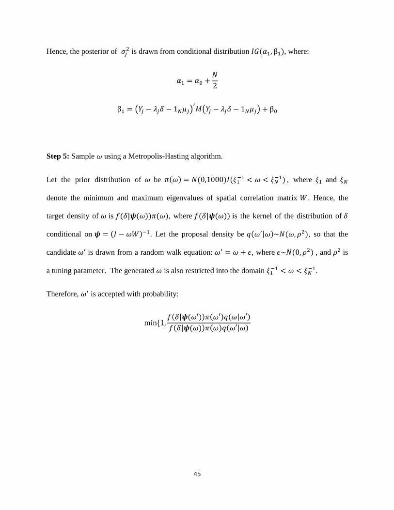
45

Hence, the posterior of 𝜎𝑗2 is drawn from conditional distribution 𝐼𝐺(𝛼1, β1), where:

𝛼1 = 𝛼0 +𝑁

2

β1 = (𝑌𝑗 − 𝜆𝑗𝛿 − 1𝑁𝜇𝑗)′𝑀(𝑌𝑗 − 𝜆𝑗𝛿 − 1𝑁𝜇𝑗) + β0

Step 5: Sample 𝜔 using a Metropolis-Hasting algorithm.

Let the prior distribution of 𝜔 be 𝜋(𝜔) = 𝑁(0,1000)𝐼(𝜉1−1 < 𝜔 < 𝜉𝑁

−1) , where 𝜉1 and 𝜉𝑁

denote the minimum and maximum eigenvalues of spatial correlation matrix 𝑊 . Hence, the

target density of 𝜔 is 𝑓(𝛿|𝝍(𝜔))𝜋(𝜔), where 𝑓(𝛿|𝝍(𝜔)) is the kernel of the distribution of 𝛿

conditional on 𝝍 = (𝐼 − 𝜔𝑊)−1. Let the proposal density be 𝑞(𝜔′|𝜔)~𝑁(𝜔, 𝜌2), so that the

candidate 𝜔′ is drawn from a random walk equation: 𝜔′ = 𝜔 + 𝜖, where 𝜖~𝑁(0, 𝜌2) , and 𝜌2 is

a tuning parameter. The generated 𝜔 is also restricted into the domain 𝜉1−1 < 𝜔 < 𝜉𝑁

−1.

Therefore, 𝜔′ is accepted with probability:

min{1,𝑓(𝛿|𝝍(𝜔′))𝜋(𝜔′)𝑞(𝜔|𝜔′)

𝑓(𝛿|𝝍(𝜔))𝜋(𝜔)𝑞(𝜔′|𝜔)

46

Appendix II: Numbering of Countries

# Country

1 Afghanistan

2 Albania

3 Algeria

4 Andorra

5 Angola

6 Antigua and Barbuda

7 Argentina

8 Armenia

9 Australia

10 Austria

11 Azerbaijan

12 Bahamas

13 Bahrain

14 Bangladesh

15 Barbados

16 Belarus

17 Belgium

18 Belize

19 Benin

20 Bhutan

21 Bolivia (Plurinational State of)

22 Bosnia and Herzegovina

23 Botswana

24 Brazil

25 Brunei Darussalam

26 Bulgaria

27 Burkina Faso

28 Burundi

29 Cambodia

30 Cameroon

31 Canada

32 Cape Verde

33 Central African Republic

34 Chad

35 Chile

36 China

37 Colombia

38 Comoros

39 Congo

40 Congo (Democratic Republic of the)

41 Costa Rica

42 Croatia

43 Cuba

44 Cyprus

45 Czech Republic

46 Côte d'Ivoire

47 Denmark

48 Djibouti

49 Dominica

50 Dominican Republic

51 Ecuador

52 Egypt

53 El Salvador

54 Equatorial Guinea

55 Eritrea

56 Estonia

57 Ethiopia

58 Fiji

59 Finland

60 France

61 Gabon

62 Gambia

63 Georgia

64 Germany

65 Ghana

66 Greece

67 Grenada

68 Guatemala

69 Guinea

70 Guinea-Bissau

71 Guyana

72 Haiti

73 Honduras

74 Hong Kong

75 Hungary

47

76 Iceland

77 India

78 Indonesia

79 Iran (Islamic Republic of)

80 Iraq

81 Ireland

82 Israel

83 Italy

84 Jamaica

85 Japan

86 Jordan

87 Kazakhstan

88 Kenya

89 Kiribati

90 Korea (Republic of)

91 Kuwait

92 Kyrgyzstan

93 Lao People's Democratic Republic

94 Latvia

95 Lebanon

96 Lesotho

97 Liberia

98 Libya

99 Liechtenstein

100 Lithuania

101 Luxembourg

102 Madagascar

103 Malawi

104 Malaysia

105 Maldives

106 Mali

107 Malta

108 Mauritania

109 Mauritius

110 Mexico

111 Micronesia (Federated States of)

112 Moldova (Republic of)

113 Mongolia

114 Montenegro

115 Morocco

116 Mozambique

117 Myanmar

118 Namibia

119 Nepal

120 Netherlands

121 New Zealand

122 Nicaragua

123 Niger

124 Nigeria

125 Norway

126 Oman

127 Pakistan

128 Palau

129 Palestine, State of

130 Panama

131 Papua New Guinea

132 Paraguay

133 Peru

134 Philippines

135 Poland

136 Portugal

137 Qatar

138 Romania

139 Russian Federation

140 Rwanda

141 Saint Kitts and Nevis

142 Saint Lucia

143 Saint Vincent and the Grenadines

144 Samoa

145 Sao Tome and Principe

146 Saudi Arabia

147 Senegal

148 Serbia

149 Seychelles

150 Sierra Leone

151 Singapore

152 Slovakia

153 Slovenia

154 Solomon Islands

155 South Africa

156 Spain

157 Sri Lanka

158 Sudan

159 Suriname

160 Swaziland

161 Sweden

48

162 Switzerland

163 Syrian Arab Republic

164 Tajikistan

165 Tanzania (United Republic of)

166 Thailand

167 The former Yugoslav Republic of Macedonia

168 Timor-Leste

169 Togo

170 Tonga

171 Trinidad and Tobago

172 Tunisia

173 Turkey

174 Turkmenistan

175 Uganda

176 Ukraine

177 United Arab Emirates

178 United Kingdom

179 United States

180 Uruguay

181 Uzbekistan

182 Vanuatu

183 Venezuela (Bolivarian Republic of)

184 Viet Nam

185 Yemen

186 Zambia

187 Zimbabwe

49

Appendix III: Figures of “Green” HDI Using Different Functional Forms

Figure A1. Posterior Mean and 99% CI of Model-based “Green” HDI Ranks

vs. Official HDI Ranks Using GNI per capita and ln(𝐂𝐎𝟐)

50

Figure A2. Posterior Mean and 99% CI of Model-based “Green” HDI Ranks

vs. Official HDI Ranks Using ln(GNI per capita) and 𝐂𝐎𝟐

51

Figure A3. Posterior Mean and 99% CI of Model-based “Green” HDI Ranks

vs. Official HDI Ranks Using ln(GNI per capita) and ln(𝐂𝐎𝟐)

52

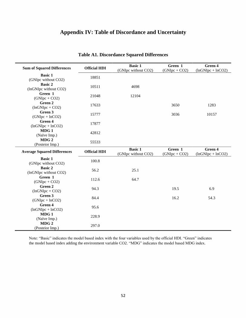
Appendix IV: Table of Discordance and Uncertainty

Table A1. Discordance Squared Differences

Sum of Squared Differences Official HDI Basic 1

(GNIpc without CO2) Green 1

(GNIpc + CO2) Green 4

(lnGNIpc + lnCO2)

Basic 1

(GNIpc without CO2) 18851

Basic 2

(lnGNIpc without CO2) 10511 4698

Green 1

(GNIpc + CO2) 21048 12104

Green 2

(lnGNIpc + CO2) 17633

3650 1283

Green 3

(GNIpc + lnCO2) 15777

3036 10157

Green 4

(lnGNIpc + lnCO2) 17877

MDG 1

(Naïve Imp.) 42812

MDG 2

(Posteior Imp.) 55533

Average Squared Differences Official HDI Basic 1

(GNIpc without CO2) Green 1

(GNIpc + CO2) Green 4

(lnGNIpc + lnCO2)

Basic 1

(GNIpc without CO2) 100.8

Basic 2

(lnGNIpc without CO2) 56.2 25.1

Green 1

(GNIpc + CO2) 112.6 64.7

Green 2

(lnGNIpc + CO2) 94.3

19.5 6.9

Green 3

(GNIpc + lnCO2) 84.4

16.2 54.3

Green 4

(lnGNIpc + lnCO2) 95.6

MDG 1

(Naïve Imp.) 228.9

MDG 2

(Posteior Imp.) 297.0

Note: “Basic” indicates the model based index with the four variables used by the official HDI. “Green” indicates

the model based index adding the environment variable CO2. “MDG” indicates the model based MDG index.

53

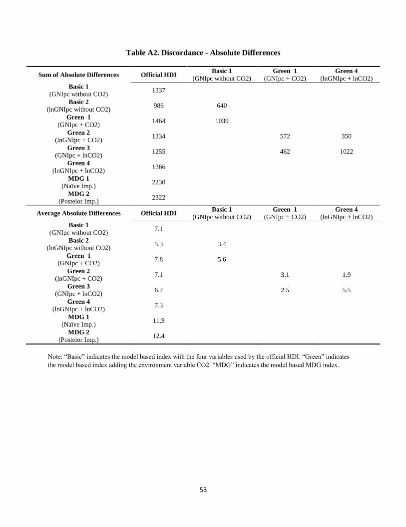
Table A2. Discordance - Absolute Differences

Sum of Absolute Differences Official HDI Basic 1

(GNIpc without CO2) Green 1

(GNIpc + CO2) Green 4

(lnGNIpc + lnCO2)

Basic 1

(GNIpc without CO2) 1337

Basic 2

(lnGNIpc without CO2) 986 640

Green 1

(GNIpc + CO2) 1464 1039

Green 2

(lnGNIpc + CO2) 1334

572 350

Green 3

(GNIpc + lnCO2) 1255

462 1022

Green 4

(lnGNIpc + lnCO2) 1366

MDG 1

(Naïve Imp.) 2230

MDG 2

(Posteior Imp.) 2322

Average Absolute Differences Official HDI Basic 1

(GNIpc without CO2) Green 1

(GNIpc + CO2) Green 4

(lnGNIpc + lnCO2)

Basic 1

(GNIpc without CO2) 7.1

Basic 2

(lnGNIpc without CO2) 5.3 3.4

Green 1

(GNIpc + CO2) 7.8 5.6

Green 2

(lnGNIpc + CO2) 7.1

3.1 1.9

Green 3

(GNIpc + lnCO2) 6.7

2.5 5.5

Green 4

(lnGNIpc + lnCO2) 7.3

MDG 1

(Naïve Imp.) 11.9

MDG 2

(Posteior Imp.) 12.4

Note: “Basic” indicates the model based index with the four variables used by the official HDI. “Green” indicates

the model based index adding the environment variable CO2. “MDG” indicates the model based MDG index.

54

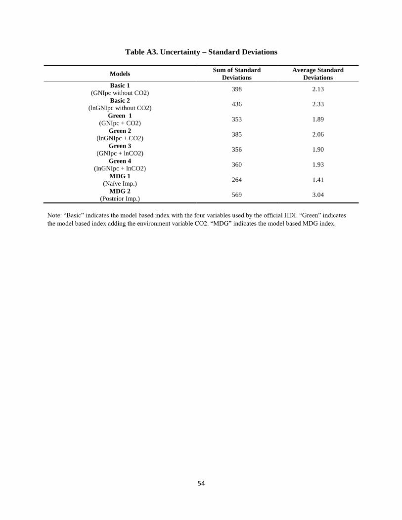
Table A3. Uncertainty – Standard Deviations

Models Sum of Standard

Deviations

Average Standard

Deviations

Basic 1

(GNIpc without CO2) 398 2.13

Basic 2

(lnGNIpc without CO2) 436 2.33

Green 1

(GNIpc + CO2) 353 1.89

Green 2

(lnGNIpc + CO2) 385 2.06

Green 3

(GNIpc + lnCO2) 356 1.90

Green 4

(lnGNIpc + lnCO2) 360 1.93

MDG 1

(Naïve Imp.) 264 1.41

MDG 2

(Posteior Imp.) 569 3.04

Note: “Basic” indicates the model based index with the four variables used by the official HDI. “Green” indicates

the model based index adding the environment variable CO2. “MDG” indicates the model based MDG index.