using statistics to make inferences 10
DESCRIPTION
Using Statistics To Make Inferences 10. Summary To fit a straight line through data. Goals Given raw data, or the appropriate sums, to fit a straight line through the data. Practical Recall last weeks practical. Perform scatter plots, evaluate correlations and add regression lines. 1. - PowerPoint PPT PresentationTRANSCRIPT

10.11
Using Statistics To Make Inferences 10
Summary To fit a straight line through data.
Goals
Given raw data, or the appropriate sums, to fit a straight line through the data.
Practical Recall last weeks practical. Perform scatter
plots, evaluate correlations and add regression lines.
Wednesday 19 April 2023 11:01 PM
10.22
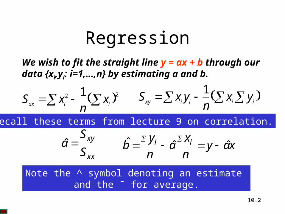
Regression We wish to fit the straight line y = ax + b through our data {xi,yi: i=1,…,n} by estimating a and b.
22 1iixx x
nxS iiiixy yx
nyxS
1
Note the ^ symbol denoting an estimate and the ¯ for average.
xx
xy
S
Sa ˆ xay
n
xa
n
yb ii ˆˆˆ
Recall these terms from lecture 9 on correlation.

10.33
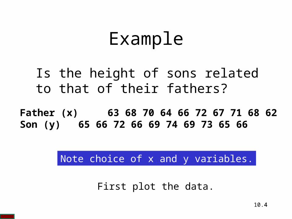
Example
Is the height of sons related to that of their fathers?
Father 63 68 70 64 66 72 67 71 68 62Son 65 66 72 66 69 74 69 73 65 66
Which is the independent (x) variable?
10.44
Example
Is the height of sons related to that of their fathers?
Father (x) 63 68 70 64 66 72 67 71 68 62Son (y) 65 66 72 66 69 74 69 73 65 66
Note choice of x and y variables.
First plot the data.
10.55
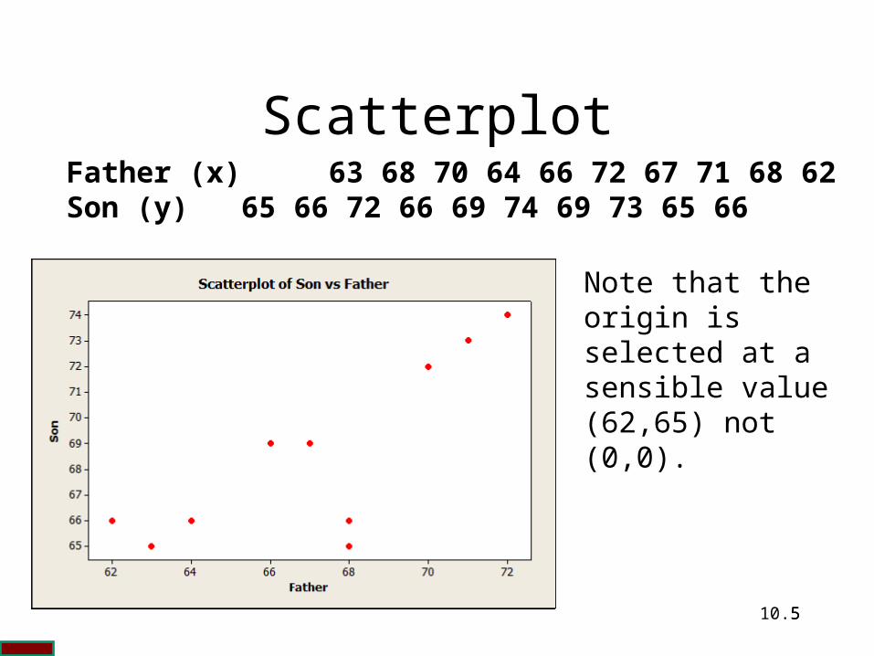
ScatterplotFather (x) 63 68 70 64 66 72 67 71 68 62Son (y) 65 66 72 66 69 74 69 73 65 66
Note that the origin is selected at a sensible value (62,65) not (0,0).
10.66
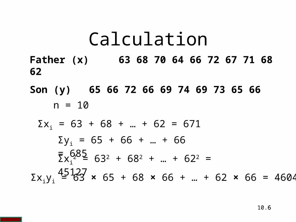
CalculationFather (x) 63 68 70 64 66 72 67 71 68 62
Son (y) 65 66 72 66 69 74 69 73 65 66
n = 10
Σxi = 63 + 68 + … + 62 = 671
Σyi = 65 + 66 + … + 66 = 685 Σxi
2 = 632 + 682 + … + 622 = 45127 Σxiyi = 63 × 65 + 68 × 66 + … + 62 × 66 = 46047

10.77
Calculation Sxx
n = 10 Σxi = 671 Σyi = 685 Σxi2 = 45127 Σxiyi =
46047
9.10210
67145127
1 222 iixx x
nxS

10.88
Calculation Sxy
n = 10 Σxi = 671 Σyi = 685 Σxi2 = 45127 Σxiyi =
46047
5.8310
68567146047
1 iiiixy yxn
yxS

10.99
Calculation Gradient an = 10 Σxi = 671 Σyi = 685 Sxx = 102.9 Sxy = 83.5
8115.09.1025.83
ˆ xx
xy
S
Sa Gradient or slope

10.1010
Calculation Intercept bn = 10 Σxi = 671 Σyi = 685
Son = 14.05 + 0.81 × Father
8115.09.1025.83
ˆ xx
xy
S
Sa
05.1410671
8115.010685
ˆˆ
nx
any
b ii
Gradient or slope
Intercept orconstant
a
Sxx = 102.9 Sxy = 83.5

10.1111
ResultsSon = 14.05 + 0.8115 × Father
To produce the line select two extreme values for the x variable.
Father
Son
727068666462
74737271706968676665
Scatterplot of Son vs FatherFather = 72 then Son = 14.05 + 0.8115 × 72 = 72.478Father = 62 then Son = 14.05 + 0.8115 × 62 = 64.363

10.1212
ResultsFather = 72 Son = 72.48 and Father = 62 Son = 64.36
Father
Son
727068666462
75.0
72.5
70.0
67.5
65.0
Fitted Line PlotSon = 14.05 + 0.8115 Father
10.1313
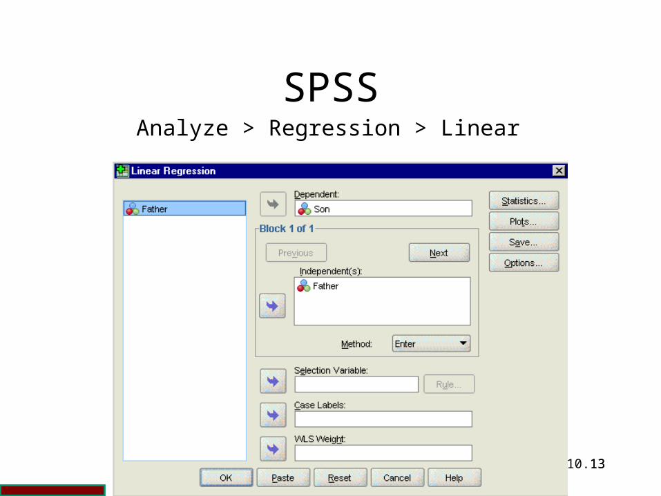
SPSSAnalyze > Regression > Linear

10.1414
SPSSSame intercept and gradient
Coefficientsa
14.051 14.573 .964 .363
.811 .217 .798 3.741 .006
(Constant)
Father
Model1
B Std. Error
UnstandardizedCoefficients
Beta
StandardizedCoefficients
t Sig.
Dependent Variable: Sona.
10.1515
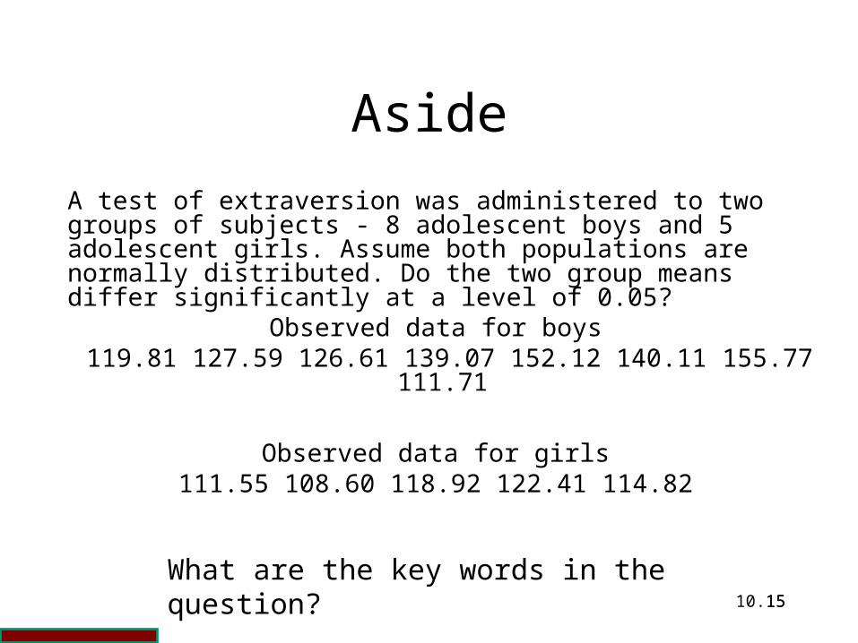
Aside
A test of extraversion was administered to two groups of subjects - 8 adolescent boys and 5 adolescent girls. Assume both populations are normally distributed. Do the two group means differ significantly at a level of 0.05?
Observed data for boys119.81 127.59 126.61 139.07 152.12 140.11 155.77
111.71
Observed data for girls111.55 108.60 118.92 122.41 114.82
What are the key words in the question?

10.1616
Aside
A test of extraversion was administered to two groups of subjects - 8 adolescent boys and 5 adolescent girls. Assume both populations are normally distributed. Do the two group means differ significantly at a level of 0.05?
Observed data for boys119.81 127.59 126.61 139.07 152.12 140.11 155.77
111.71
Observed data for girls111.55 108.60 118.92 122.41 114.82
CCCCCCCCCCCc
10.1717
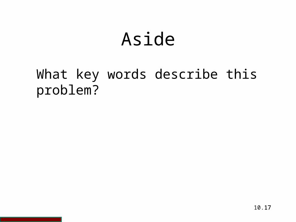
Aside
What key words describe this problem?

10.1818
Aside
two samplecomparison of means
Which tests might be appropriate?

10.1919
Aside
z or tWhich is appropriate here?
Since σ is not available we use a two sample t test.
CCCCCCCc
10.2020
Example
On 28 January 1986, the space shuttle Challenger was launched at a temperature of 31°F. The ensuing catastrophe was caused by a combustion gas leak through a joint in one of the booster rockets, which was sealed by a device called an O-ring. The data (in the print version of the notes) relate launch temperature to the number of O-rings under thermal distress for 24 previous launches.

10.2121
Challenger's Rollout From Orbiter Processing Facility To
The Vehicle Assembly Building

10.2222
The Crew Of The Final, Ill-fated Flight Of The Challenger

10.2323
The Challenger Breaks Apart 73 Seconds Into Its Final
Mission

10.2424
Debris Recovered From Space Shuttle Challenger

10.2525
Example
On January 28, 1986, the space shuttle Challenger was launched at a temperature of 31°F. The ensuing catastrophe was caused by a combustion gas leak through a joint in one of the booster rockets, which was sealed by a device called an O-ring. The data (in the print version of the notes) relate launch temperature to the number of O-rings under thermal distress for 24 previous launches.
First plot the data.Variables are number of rings that fail and temperature.Which is independent?

10.2626
Scatterplot
Temperature (°F)Num
ber
of O
Rin
gs
that
fail
80757065605550
3
2
1
0

10.2727
Calculation SxxHere the independent variable is Temp (x) and the dependent variable is Ring (y)
120024
1680118800
1 222 iixx x
nxS
n = 24 ΣTempi = 1680 ΣRingi = 10
ΣTempi2 = 118800 ΣTempi Ringi = 627

10.2828
Calculation Sxy
Here the independent variable is Temp (x) and the dependent variable is Ring (y)
7310
101680627
1 iiiixy yxn
yxS
n = 24 ΣTempi = 1680 ΣRingi = 10
ΣTempi2 = 118800 ΣTempi Ringi = 627

10.2929
Calculation Gradient a
n = 24 ΣTempi = 1680 ΣRingi = 10
0608.01200
73ˆ
xx
xy
S
Sa
Sxx = 1200 Sxy = -73

10.3030
Calculation Intercept b
n = 24 ΣTempi = 1680 ΣRingi = 10
1200xxS 73xyS
0608.01200
73ˆ
xx
xy
S
Sa
6750.4168024
0608.0
24
10ˆ1ˆ iix
n
ay
nb
10.3131
Results
Temperature (°F)
Num
ber
of O
Rin
gs
that fa
il
80757065605550
3
2
1
0
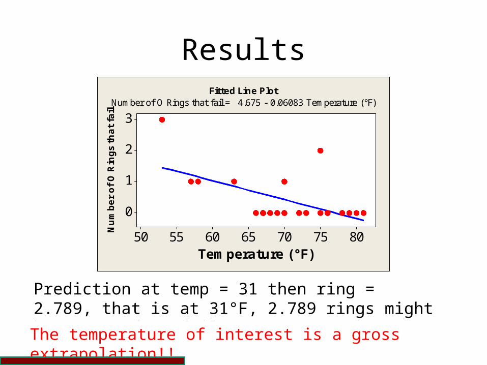
Fitted Line PlotNumber of O Rings that fail = 4.675 - 0.06083 Temperature (°F)
Prediction at temp = 31 then ring = 2.789, that is at 31°F, 2.789 rings might be expected to fail!
The temperature of interest is a gross extrapolation!!

10.3232
Conclusion
Richard Phillips Feynman (May 11, 1918 – February 15, 1988) was an American physicist known for his work in the path integral formulation of quantum mechanics, the theory of quantum electrodynamics, and the physics of the superfluidity of supercooled liquid helium, as well as in particle physics. For his contributions to the development of quantum electrodynamics, Feynman, jointly with Julian Schwinger and Sin-Itiro Tomonaga, received the Nobel Prize in Physics in 1965.

10.3333
Conclusion
Feynman played an important role on the Presidential Rogers Commission, which investigated the Challenger disaster. During a televised hearing, Feynman demonstrated that the material used in the shuttle's O-rings became less resilient in cold weather by immersing a sample of the material in ice-cold water. The Commission ultimately determined that the disaster was caused by the primary O-ring not properly sealing due to extremely cold weather at Cape Canaveral.

10.3434
SPSSSame intercept and gradient
Coefficientsa
4.675 1.327 3.523 .002
-.061 .019 -.567 -3.225 .004
(Constant)
Temp
Model1
B Std. Error
UnstandardizedCoefficients
Beta
StandardizedCoefficients
t Sig.
Dependent Variable: Ringa.

10.3535
SPSSScatter plots/Regression
Graphs > Legacy Dialogs > Scatter/Dot
Simple scatter

10.3636
SPSS
10.3737
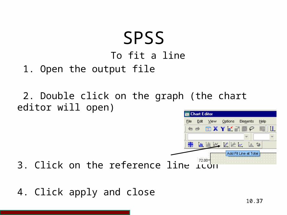
SPSSTo fit a line
1. Open the output file
2. Double click on the graph (the chart editor will open)
3. Click on the reference line icon
4. Click apply and close

10.3838
SPSS

10.3939
What Is Multiple Regression?
An example of performing a multiple regression in SPSS is now presented. Multiple regression is a statistical technique that allows the prediction of a score on one variable on the basis of the scores on several other variables.

10.4040
How Does Multiple Regression Relate To
Correlation? In a previous section you met correlation and the regression line. If two variables are correlated, then knowing the score on one variable will allow you to predict the score on the other variable. The stronger the correlation, the closer the scores will fall to the regression line and therefore the more accurate the prediction.
10.4141
How Does Multiple Regression Relate To
Correlation? Multiple regression is simply an extension of this principle, where one variable is predicted on the basis of several other variables. Having more than one independent variable is useful when predicting human behaviour, as actions, thoughts and emotions are all likely to be influenced by some combination of several factors. Using multiple regression theories (or models) can be tested about precisely which set of variables is influencing behaviour.

10.4242
When Should I Use Multiple Regression?
1. You can use this statistical technique when exploring linear relationships between dependent and independent variables – that is, when the relationship follows a straight line.

10.4343
When Should I Use Multiple Regression?
2. The dependent variable that you are seeking to predict should be measured on a continuous scale (such as interval or ratio scale). There is a separate regression method called logistic regression that can be used for dichotomous dependent variables.
10.4444
When Should I Use Multiple Regression?
3. The independent variables that you select should be measured on a ratio, interval, or ordinal scale. A nominal independent variable is legitimate but only if it is dichotomous, i.e. there are no more than two categories.

10.4545
When Should I Use Multiple Regression?
For example, sex is acceptable (where male is coded as 1 and female as 0) but gender identity (masculine, feminine and androgynous) could not be coded as a single variable. Instead, you would create three different variables each with two categories (masculine/not masculine; feminine/not feminine and androgynous/not androgynous). The term dummy variable is used to describe this type of dichotomous variable.

10.4646
When Should I Use Multiple Regression?
4. Multiple regression requires a large number of observations. The number of cases (participants) must substantially exceed the number of independent variables you are using in your regression. The absolute minimum is that you have five times as many participants as independent variables. A more acceptable ratio is 10:1, but some people argue that this should be as high as 40:1 for some statistical selection methods.

10.4747
Terminology
There are certain terms that need to clarifying to allow you to understand the results of this statistical technique.

10.4848
Beta (standardised regression coefficients)
The beta value is a measure of how strongly each independent variable influences the dependent variable. The beta is measured in units of standard deviation. For example, a beta value of 2.5 indicates that a change of one standard deviation in the independent variable will result in a change of 2.5 standard deviations in the dependent variable. Thus, the higher the beta value the greater the impact of the independent variable on the dependent variable.

10.4949
Beta (standardised regression coefficients)
When you have only one independent variable in your model, then beta is equivalent to the correlation coefficient between the independent and the dependent variable. When you have more than one independent variable, you cannot compare the contribution of each independent variable by simply comparing the correlation coefficients. The beta regression coefficient is computed to allow you to make such comparisons and to assess the strength of the relationship between each independent variable to the dependent variable.
10.5050
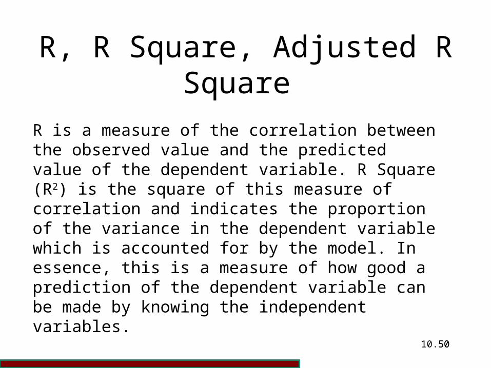
R, R Square, Adjusted R Square
R is a measure of the correlation between the observed value and the predicted value of the dependent variable. R Square (R2) is the square of this measure of correlation and indicates the proportion of the variance in the dependent variable which is accounted for by the model. In essence, this is a measure of how good a prediction of the dependent variable can be made by knowing the independent variables.

10.5151
R, R Square, Adjusted R Square
However, R square tends to somewhat over-estimate the success of the model when applied to the real world. An Adjusted R Square value is calculated which takes into account the number of variables in the model and the number of observations (participants) the model is based on. This Adjusted R Square value gives the most useful measure of the success of the model. If, for example an Adjusted R Square value of 0.75 it can be said that the model has accounted for 75% of the variance in the dependent variable.
10.5252
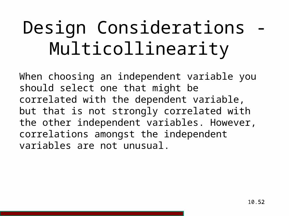
Design Considerations - Multicollinearity
When choosing an independent variable you should select one that might be correlated with the dependent variable, but that is not strongly correlated with the other independent variables. However, correlations amongst the independent variables are not unusual.

10.5353
Design Considerations - Multicollinearity
The term multicollinearity (or collinearity) is used to describe the situation when a high correlation is detected between two or more independent variables. Such high correlations cause problems when trying to draw inferences about the relative contribution of each independent variable to the success of the model. SPSS provides you with a means of checking for this and it is described below.

10.5454
Example Study
Brace, Kemp and Snelgar 2012 SPSS for Psychologists ISBN: 9780230362727 introduced the following example. In an investigation of children’s spelling Corriene Reed, decided to look at the importance of several psycholinguistic variables on spelling performance. Previous research has shown that age of acquisition has an effect on children’s reading and also on object naming.

10.5555
Example Study
A total of 64 children, aged between 7 and 9 years, completed standardised reading and spelling tests and were then asked to spell 48 words that varied systematically according to certain features such as age of acquisition, word frequency, word length, and imageability. Word length and age of acquisition emerged as significant independents of whether the word was likely to be spelt correctly.

10.5656
Example Study
Further analysis was conducted on the data to determine whether the spelling performance on this list of 48 words accurately reflected the children’s spelling ability as estimated by a standardised spelling test. Children’s chronological age, their reading age, their standardised reading score and their standardised spelling score were chosen as the independent variables. The dependent variable was the percentage correct spelling score attained by each child using the list of 48 words.

10.5757
Example Study
The aim is to reproduce some of the findings from the analysis. As you will see, the standardised spelling score derived from a validated test emerged as strongly independent of the spelling score achieved on the word list. The data file employed contains only a subset of the data collected and is used here to demonstrate multiple regression.

10.5858
How To Perform The Test
Within SPSS selectAnalyze > Regression > Linear

10.5959
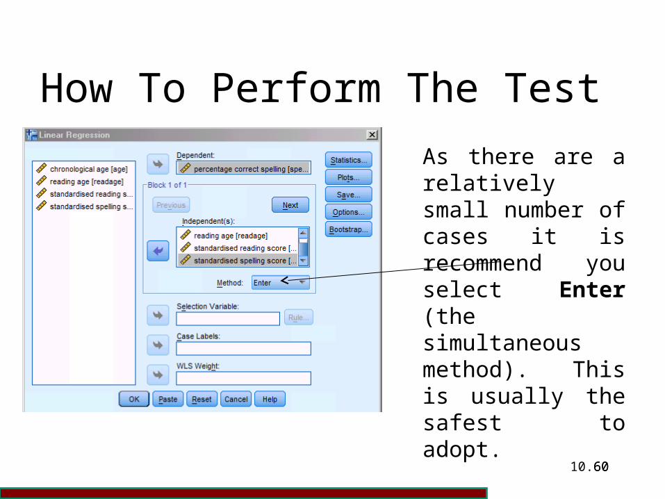
How To Perform The Test
You will then be presented with the Linear Regression dialogue box shown below. You now need to select the dependent and the independent variables. The percentage correct spelling score (“spelperc”) is chosen as the independent variable. As the dependent variables, chronological age (“age”), reading age (“readage”), standardised reading score (“standsc”), and standardised spelling score (“spellsc”) are chosen.
10.6060
How To Perform The Test
As there are a relatively small number of cases it is recommend you select Enter (the simultaneous method). This is usually the safest to adopt.

10.6161
How To Perform The Test
Now click on the Statistics button. This will bring up the Linear Regression: Statistics dialogue box shown.

10.6262
How To Perform The Test
The Collinearity diagnostics (Collinearity – a high correlation is detected between two or more independent variables) option (employed below) gives some useful additional output that allows you to assess whether you have a problem with collinearity in your data. The R squared change option (not considered here) is useful if you have selected a statistical method such as stepwise as it makes clear how the power of the model changes with the addition or removal of a independent variable from the model.

10.6363
How To Perform The Test
When you have selected the statistics options you require, click on the Continue button. This will return you to the Linear Regression dialogue box. Now click on the OK button. The output that will be produced is illustrated below.
10.6464
How To Perform The Test
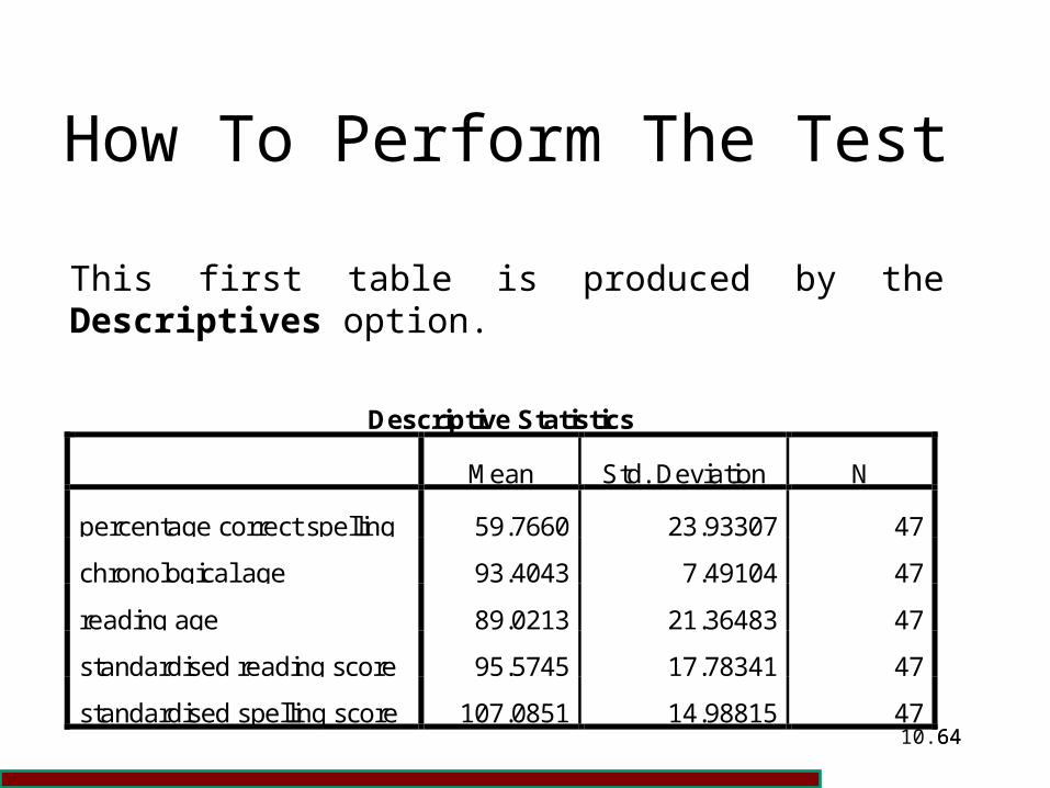
This first table is produced by the Descriptives option.
Descriptive Statistics
Mean Std. Deviation N
percentage correct spelling 59.7660 23.93307 47
chronological age 93.4043 7.49104 47
reading age 89.0213 21.36483 47
standardised reading score 95.5745 17.78341 47
standardised spelling score 107.0851 14.98815 47

10.6565
How To Perform The Test
This second table gives details of the correlation between each pair of variables. Strong correlations between the dependent and the independent variables are not ideal. The values here are acceptable.
(see the next slide)

10.6666
How To Perform The Test Correlations
percentage
correct spelling
chronological
age reading age
standardised
reading score
standardised
spelling score
percentage correct spelling 1.000 -.074 .623 .778 .847
chronological age -.074 1.000 .124 -.344 -.416
reading age .623 .124 1.000 .683 .570
standardised reading score .778 -.344 .683 1.000 .793
Pearson Correlation
standardised spelling score .847 -.416 .570 .793 1.000
percentage correct spelling . .311 .000 .000 .000
chronological age .311 . .203 .009 .002
reading age .000 .203 . .000 .000
standardised reading score .000 .009 .000 . .000
Sig. (1-tailed)
standardised spelling score .000 .002 .000 .000 .
percentage correct spelling 47 47 47 47 47
chronological age 47 47 47 47 47
reading age 47 47 47 47 47
standardised reading score 47 47 47 47 47
N
standardised spelling score 47 47 47 47 47

10.6767
How To Perform The Test
This third table tells us about the independent variables and the method used. All of the independent variables were entered simultaneously (because the Enter method was selected).
Variables Entered/Removedb
Variables
Entered
Variables
Removed Method
standardised
spelling score,
chronological
age, reading
age,
standardised
reading score
. Enter
a. All requested variables entered.
b. Dependent Variable: percentage correct spelling

10.6868
How To Perform The Test
This table is important. The Adjusted R Square value tells us that the model accounts for 83.8% of variance in the spelling scores – a very good model!
Model Summary
Model R R Square
Adjusted R
Square
Std. Error of the
Estimate
1 .923a .852 .838 9.63766
a. Predictors: (Constant), standardised spelling score, chronological
age, reading age, standardised reading score

10.6969
How To Perform The Test
This table reports an ANOVA, which assesses the overall significance of our model. As p < 0.0005 the model is significant.
ANOVAb
Model Sum of Squares df Mean Square F Sig.
Regression 22447.277 4 5611.819 60.417 .000a
Residual 3901.149 42 92.884
1
Total 26348.426 46
a. Predictors: (Constant), standardised spelling score, chronological age, reading age,
standardised reading score
b. Dependent Variable: percentage correct spelling

10.7070
How To Perform The Test
The Standardized Beta Coefficients give a measure of the contribution of each variable to the model. A large value indicates that a unit change in this independent variable has a large effect on the dependent variable. The t and Sig (p) values give a rough indication of the impact of each independent variable – a big absolute t value and small p value suggests that an independent variable is having a large impact on the dependent variable. If you requested Collinearity diagnostics these will also be included in this table – see below.
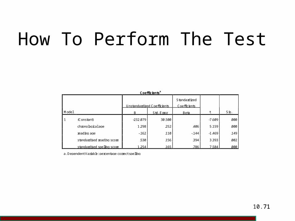
10.7171
How To Perform The Test
Coefficientsa
Unstandardized Coefficients
Standardized
Coefficients
Model B Std. Error Beta t Sig.
(Constant) -232.079 30.500 -7.609 .000
chronological age 1.298 .252 .406 5.159 .000
reading age -.162 .110 -.144 -1.469 .149
standardised reading score .530 .156 .394 3.393 .002
1
standardised spelling score 1.254 .165 .786 7.584 .000
a. Dependent Variable: percentage correct spelling

10.7272
Collinearity diagnostics
If you requested the optional Collinearity diagnostics, these will be shown in an additional two columns of the Coefficients table (the last table shown above) and a further table (titled Collinearity diagnostics) that is not shown here. Ignore this extra table and simply look at the two new columns.

10.7373
Collinearity diagnostics
Coefficientsa
Unstandardized Coefficients
Standardized
Coefficients Collinearity Statistics
Model B Std. Error Beta t Sig. Tolerance VIF
(Constant) -232.079 30.500 -7.609 .000
chronological age 1.298 .252 .406 5.159 .000 .568 1.759
reading age -.162 .110 -.144 -1.469 .149 .365 2.737
standardised reading score .530 .156 .394 3.393 .002 .262 3.820
1
standardised spelling score 1.254 .165 .786 7.584 .000 .329 3.044
a. Dependent Variable: percentage correct spelling
10.7474
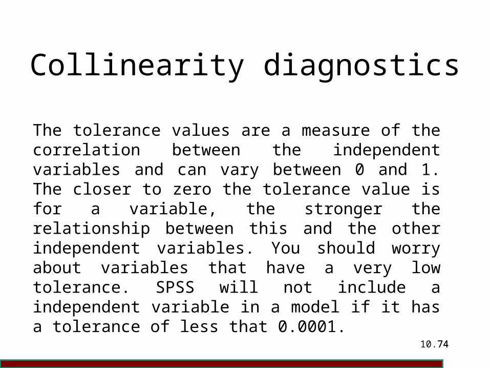
Collinearity diagnostics
The tolerance values are a measure of the correlation between the independent variables and can vary between 0 and 1. The closer to zero the tolerance value is for a variable, the stronger the relationship between this and the other independent variables. You should worry about variables that have a very low tolerance. SPSS will not include a independent variable in a model if it has a tolerance of less that 0.0001.

10.7575
Collinearity diagnostics
However, you may want to set your own criteria rather higher – perhaps excluding any variable that has a tolerance level of less than 0.01. The Variance Inflation Factor (VIF) is an alternative measure of collinearity (in fact it is the reciprocal of tolerance) in which a large value indicates a strong relationship between independent variables.

10.7676
Reporting The Results
When reporting the results of a multiple regression analysis, you want to inform the reader about the proportion of the variance accounted for by your model, the significance of your model and the significance of the independent variables. Write in the results section:

10.7777
Reporting The Results
Using the enter method, a significant model emerged (F4,42=60.417, p < 0.0005. Adjusted R square = .838). Significant variables are shown below:
I ndependent Variable Beta p
Chronological age .406 p < 0.0005
Standardised reading score .394 p = 0.002
Standardised spelling score .786 p < 0.0005
Reading age was not a significant independent in this model.

10.7878
Future Lectures
During the last week of the course there will be no formal lecture.
During the lecture session I will review previous examinations with questions proposed by the audience.

10.7979
Read
Read Howitt and Cramer pages 75-82
Read Russo (e-text) pages 202-213
Read Davis and Smith pages 173-192

10.8080
Whoops!
Souvenir mugs misspell Obama's name
Telegraph 07 Jun 2010
Australia's parliamentary gift shop has withdrawn commemorative mugs that misspelt President Barack Obama's name.

10.8181
Whoops!
Up to 69 you have a one in six chance of getting cancer. After 70 it drops to one in three.
BBC News website
5 February 2008

10.8282
Whoops!
TextReviews LLC is driven by a team of experienced publishing professionals, sales executives, marketers, and software developers. Review Summary of “Statitics for the Behavioral and Social Sciences: A Brief Course 5/e” Pearson
Accessed 17 April 2012
# Question
13 Using the following scale, please rate how well this table of contents appears to cover the topics you consider essential for your course.
Answer
A
B
C
D
F