Using Supertasks to Improve Processor Utilization in

Multiprocessor Real-time Systems∗

Philip Holman and James H. Anderson

Department of Computer Science

University of North Carolina

Chapel Hill, NC 27599-3175

E-mail: {holman,anderson}@cs.unc.edu

December 2002

Abstract

We revisit the problem of supertasking in Pfair-scheduled multiprocessor systems. In this approach, a set

of tasks, called component tasks, is assigned to a server task, called a supertask , which is then scheduled as an

ordinary Pfair task. Whenever a supertask is scheduled, its processor time is allocated to its component tasks

according to an internal scheduling algorithm. Hence, supertasking is an example of hierarchal scheduling.

In this paper, we present a generalized “reweighting” algorithm. The goal of reweighting is to assign

a fraction of a processor to a given supertask so that all timing requirements of its component tasks are

met. The generalized reweighting algorithm we present breaks new ground in three important ways. First,

component tasks are permitted to have non-integer execution costs. Consequently, supertasking can now be

used to ameliorate schedulability loss due to the integer-cost assumption of Pfair scheduling. To the best of

our knowledge, no other techniques have been proposed to address this problem. Second, blocking terms are

included in the analysis. Since blocking terms are used to account for a wide range of behaviors commonly

found in actual systems (e.g., non-preemptivity, resource sharing, deferrable execution, etc.), their inclusion

is a necessary step towards utilizing supertasks in practice. Finally, the scope of supertasking has been

extended by employing a more flexible global-scheduling model. This added flexibility allows supertasks to

be utilized in systems that do not satisfy strict Pfairness. To demonstrate the efficacy of the supertasking

approach, we present an experimental evaluation of our algorithm that suggests that reweighting may often

result in almost no schedulability loss in practice.

∗Work supported by NSF grants CCR 9972211, CCR 9988327, and ITR 0082866.

1 Introduction

Multiprocessor scheduling techniques fall into two general categories: partitioning and global scheduling . In

the partitioning approach, each processor schedules tasks independently from a local ready queue. In contrast,

all ready tasks are stored in a single queue under global scheduling and interprocessor migration is allowed.

Presently, partitioning is the favored approach, largely because well-understood uniprocessor scheduling algo-

rithms can be used for per-processor scheduling. Despite its popularity, the partitioning approach is inherently

suboptimal when scheduling periodic tasks. A well-known example of this is a two-processor system that con-

tains three synchronous periodic tasks, each with an execution cost of 2 and a period of 3. Completing each job

before the release of its successor is impossible in such a system without migration.

One particularly promising global-scheduling approach is proportionate-fair (Pfair) scheduling, first proposed

by Baruah et al. [1]. Pfair scheduling is presently the only known optimal method for scheduling recurrent tasks

in a multiprocessor system. Under Pfair scheduling, each task is assigned a weight , w, that specifies the rate at

which it should execute. Tasks are scheduled using a fixed-size allocation quantum so that each task’s actual

allocation over any time interval [0, L) is strictly within one quantum of its ideal allocation, w · L.Unfortunately, in prior work on Pfair scheduling, it is assumed that all execution costs are expressed as

multiples of the quantum size. Consequently, the theoretical optimality of Pfair scheduling hinges on the

assumption that the quantum size can be made arbitrarily small. In actual systems, practical factors, such as

context-switching and scheduling overhead, impose an implicit lower bound on the quantum size. When the

quantum size is restricted, Pfair scheduling algorithms are not optimal. For instance, a periodic task with a

worst-case execution time of 11 ms would need to reserve 20 ms of processor time in a Pfair-scheduled system

that uses a 10-ms quantum. Such an inflated reservation results in considerable schedulability loss. Although

context-switching and migration overhead is the most common criticism of Pfair scheduling, recent experimental

work [7] suggests that this integer-cost problem is actually a more serious concern.

Hybrid Approach. In recent work, we investigated the use of supertasks in Pfair-scheduled systems [3].

Under supertasking, a set of tasks, called component tasks , is assigned to a server task, called a supertask ,

which is then scheduled as an ordinary Pfair task. Whenever a supertask is scheduled, its processor time is

allocated to its component tasks according to an internal scheduling algorithm.

Although a supertask should ideally be assigned a weight equal to the cumulative utilization of its component

tasks, Moir and Ramamurthy [5] demonstrated that the timing requirements of component tasks may be violated

when using such an assignment. In prior work [3], we proved that such violations can be avoided by using a

more pessimistic weight assignment. Unfortunately, this prior work suggests that reweighting will almost always

result in schedulability loss. However, empirical data presented later suggests that this loss should be very small

(and often negligible) in practice.

Although conceptually similar to partitioning, supertasking provides more flexibility when selecting task

1

assignments. Whereas the number of processors and their capacities are fixed under partitioning, the number

of supertasks and their capacities are not. Indeed, supertask capacities (i.e., weights) can be assigned after

making task assignments. This weight-assignment problem is referred to as the reweighting problem. For the

purpose of assigning tasks, each supertask can temporarily be granted a unit capacity (weight). Following the

assignment of tasks, these weights can then be reduced to minimize schedulability loss.

Furthermore, supertasking can be used to ameliorate schedulability loss due to the integer-cost problem.

By packing tasks into supertasks and using a uniprocessor scheduling algorithm that does not require integer

execution costs, loss due to the integer-cost problem can be traded for loss due to reweighting. Later, we

present empirical evidence that shows the efficacy of this trade-off. Indeed, the results presented later suggest

that reweighting may often result in almost no schedulability loss in practice.

Contributions of this Paper. Unfortunately, the theory of supertasking has not been sufficiently developed

to permit its use in practice. In prior work on supertasking [3, 5], it has been assumed that the global scheduler

respects strict Pfairness, that component tasks have integer execution costs, and that component tasks are

independent. These latter two assumptions are obviously unrealistic. Furthermore, there has been recent

interest in applying Pfair scheduling with relaxed scheduling constraints [2, 8]. This interest stems from the

fact that relaxing scheduling constraints typically permits the use of simpler algorithms, which, in turn, reduces

overhead. For instance, our prior work on supertasks proved that allowing component tasks to experience

bounded deadline misses can result in substantial schedulability gains [3].

In this paper, we present a generalized reweighting algorithm that extends our prior work on reweighting in

the following three ways: (i) execution costs are no longer assumed to be integral; (ii) the global-scheduling

model supports the use of relaxed fairness constraints; (iii) blocking terms are included in the analysis. In

addition to the reasons given above, these three extensions are important because many task behaviors commonly

encountered in practice, such as blocking and self-suspension, can disrupt fair allocation rates and hence are

problematic under fair scheduling. By utilizing supertasks, tasks exhibiting such behaviors can be grouped

together and scheduled using unfair uniprocessor algorithms, resulting in considerably less schedulability loss.

The remainder of the paper is organized as follows. Sec. 2 summarizes background information and notational

conventions. In Sec. 3, the reweighting condition used in our analysis is derived. Our reweighting algorithm is

then presented and analyzed in Secs. 4 and 5. Sec. 6 contains experimental results that demonstrate the efficacy

of using supertasks to reduce schedulability loss. We conclude in Sec. 7.

2 Background

Given a set of component tasks τ , our goal is to compute the smallest weight that can be assigned to the

corresponding supertask S so that the schedulability of τ is ensured. (We will precisely define the schedulability

2

0 5 10 15 20

T1

T2

T3

T4

T5

T6

(a) Strict Pfairness

Strict Pfairness

Lag & WindowRelaxed

LEGEND

Lag Relaxed

0 5 10 15 20

T1

T3

T6

T2

T4

T5

(b) Relaxed Pfairness

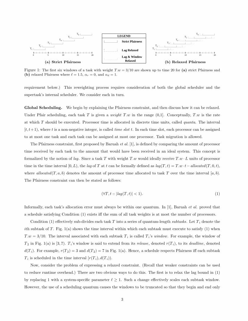
Figure 1: The first six windows of a task with weight T.w = 3/10 are shown up to time 20 for (a) strict Pfairness and(b) relaxed Pfairness where � = 1.5, αr = 0, and αd = 1.

requirement below.) This reweighting process requires consideration of both the global scheduler and the

supertask’s internal scheduler. We consider each in turn.

Global Scheduling. We begin by explaining the Pfairness constraint, and then discuss how it can be relaxed.

Under Pfair scheduling, each task T is given a weight T .w in the range (0,1]. Conceptually, T .w is the rate

at which T should be executed. Processor time is allocated in discrete time units, called quanta. The interval

[t, t+1), where t is a non-negative integer, is called time slot t. In each time slot, each processor can be assigned

to at most one task and each task can be assigned at most one processor. Task migration is allowed.

The Pfairness constraint, first proposed by Baruah et al. [1], is defined by comparing the amount of processor

time received by each task to the amount that would have been received in an ideal system. This concept is

formalized by the notion of lag . Since a task T with weight T .w would ideally receive T .w ·L units of processortime in the time interval [0, L), the lag of T at t can be formally defined as lag(T , t) = T .w · t−allocated(T , 0, t),

where allocated(T, a, b) denotes the amount of processor time allocated to task T over the time interval [a, b).

The Pfairness constraint can then be stated as follows:

(∀T , t :: |lag(T , t)| < 1). (1)

Informally, each task’s allocation error must always be within one quantum. In [1], Baruah et al. proved that

a schedule satisfying Condition (1) exists iff the sum of all task weights is at most the number of processors.

Condition (1) effectively sub-divides each task T into a series of quantum-length subtasks. Let T i denote the

ith subtask of T . Fig. 1(a) shows the time interval within which each subtask must execute to satisfy (1) when

T .w = 3/10. The interval associated with each subtask T i is called T i’s window . For example, the window of

T 2 in Fig. 1(a) is [3, 7). T i’s window is said to extend from its release, denoted r(T i), to its deadline, denoted

d(T i). For example, r(T 2) = 3 and d(T 2) = 7 in Fig. 1(a). Hence, a schedule respects Pfairness iff each subtask

T i is scheduled in the time interval [r(T i), d(T i)).

Now, consider the problem of expressing a relaxed constraint. (Recall that weaker constraints can be used

to reduce runtime overhead.) There are two obvious ways to do this. The first is to relax the lag bound in (1)

by replacing 1 with a system-specific parameter � ≥ 1. Such a change effectively scales each subtask window.

However, the use of a scheduling quantum causes the windows to be truncated so that they begin and end only

3

on slot boundaries. As a result, this scaling may not be uniform across all subtasks, as shown in Fig. 1(b). In

this figure, � = 1.5. Notice that the windows of T 2, T 3, and T 4 are each affected differently by the scaling.

Alternatively, the Pfairness constraint can be relaxed by applying a uniform extension to all windows. Let

αr and αd denote the maximum number of slots by which each window’s release and deadline, respectively, are

extended. (Assume that αr and αd are non-negative integers.) Fig. 1(b) illustrates the case in which � = 1.5,

αr = 0, and αd = 1. Note that each window’s deadline is extended one slot beyond its lag-based placement.

To avoid confusion, we will refer to the window obtained by using αr and αd as the extended window of the

subtask. For example, T 2 has a deadline at time 9 and an extended deadline at time 10 in Fig. 1(b). As shown

below, only the sum of these parameters, α = αr + αd, will be important when reweighting.

The following theorem formally expresses the impact � and α have on the amount of time available to

component tasks over any interval of time.

Theorem 1 Any task T with weight T .w executing in a relaxed Pfair-scheduled system characterized by �, αr,

and αd will receive at least max(0, T .w · (L− α)− 2��+ 1) quanta of execution time over each slot interval of

length L, where L is any non-negative integer and α = αr + αd.

Proof. When αr = αd = 0, the lag bound implies that |allocated(T , 0, u) − T .w · u| < � must hold at every

time u. Since allocated(T , 0, u) is always an integer at slot boundaries, this bound can be rewritten as shown

below when u corresponds to a slot boundary.

T .w · u− ��+ 1 ≤ allocated(T , 0, u) ≤ T .w · u+ �� − 1

Informally, T .w ·u− ��+1 (respectively, T .w ·u+ ��−1) is the number of subtasks with deadlines at or before(respectively, with releases before) integer time u.

However, a subtask with a deadline at d that is scheduled under relaxed window constraints may not complete

until its extended deadline at time d+αd. Thus, subtasks with deadlines after u−αd should not be counted in

the lower bound. Similarly, subtasks with releases before u + αr may have been scheduled before u and hence

should be counted in the upper bound. These adjustments yield the following bounds:

T .w · (u− αd)− ��+ 1 ≤ allocated(T , 0, u) ≤ T .w · (u+ αr) + �� − 1. (2)

The derivation given below completes the proof.

allocated(T , t, t+ L)

= allocated(T , 0, t+ L)− allocated(T , 0, t) , by definition

≥ [T .w · (t+ L− αd)− ��+ 1]− [ T .w · (t+ αr) + �� − 1] , by (2)

4

= T .w · (t+ αr) + �+ T .w · (L− α)− 2�� − T .w · (t+ αr) + ��+ 2 , rewriting

≥ T .w · (L− α)− 2��+ 1 , a+ b� ≥ a�+ b� − 1 ✷

Local Scheduling. We assume that τ (the set of component tasks under consideration) consists solely of N

periodic or sporadic tasks. Each sporadic (respectively, periodic) task T is characterized by the tuple (θ, e, p),

where T .e is the execution requirement of each job, T .p is the minimum (respectively, exact) separation between

consecutive jobs releases, and θ is the release time of the first job. (θ is mentioned here only for completeness; it

will not be needed in our analysis.) We assume that all job releases and deadlines of component tasks coincide

with slot boundaries. We further assume that each such task has a tardiness threshold T .c, which is the allowable

difference between a job’s completion time and its deadline. Hence, T ’s jobs have hard deadlines when T .c = 0

and soft deadlines otherwise. (Whereas relaxed fairness constraints can be exploited to reduce global-scheduling

overhead, tardiness thresholds can be used to reduce the schedulability loss caused by reweighting.) Based on

these parameters, we can formally state the component-task schedulability condition. τ is said to be schedulable

by S with respect to some component-task scheduling algorithm σ (defined below) if and only if for all tasks T

in τ and for all jobs of T , the tardiness of the job does not exceed T .c in the schedule produced by σ.

We now define σ. A job of task T with an absolute deadline at d can be considered to have an effective

deadline at time d+T .c due to the use of tardiness thresholds. Hence, an earliest-effective-deadline-first (EEDF)

policy is the obvious choice for σ. Under this policy, jobs with earlier effective deadlines are given higher priority.

To simplify the presentation of our results, we define a few shorthand notations. Let T .u = T .e/T .p denote

the utilization of T , and let U denote the sum of these values across all tasks in τ . Also, let τ(L) denote the

subset of τ consisting only of tasks with tardiness thresholds at most L.

3 Reweighting Problem

In this section, we present the reweighting problem and discuss some of its characteristics.

Deriving a Reweighting Condition. Suppose that τ is scheduled using EEDF priorities and that some

job J of task T both violates its tardiness threshold and is the first job to do so. Let tr (respectively, td) be

the release (respectively, deadline) of J . Due to the violation, there must exist an interval I = [t, t+ L), where

t ≤ tr and t + L = td + T .c, such that the total demand for processing time exceeded the available processing

time, as expressed in (3).

demand(τ , T , I) > available(I) (3)

For simplicity, we henceforth assume that t falls on a slot boundary, which implies that L is an integer.1

1In most cases, this assumption should hold. When it does not, we can still derive a necessary condition for a timing violationof the form given by (3) by manipulating the form of the blocking term, which is introduced below.

5

Under EEDF scheduling, demand(τ , T , I) can be expressed as a combination of two terms. First, processor

time is demanded by all jobs with releases at or after t and effective deadlines at or before t+ L. Each task T ′

has at most max(L − T ′.c, 0)/T ′.p� such jobs in any interval of length L. (When T ′ is a sporadic task, this

bound is tight.) The second term is a generic “blocking” term, denoted b(τ , T , L), which accounts for all other

forms of demand.2 Since the form of b(τ , T , L) will be system-specific, we simply assume for now that b(τ , T , L)

is an arbitrary function. Using these two terms leads to the following inequality:

demand(τ , T , I) ≤∑

T ′∈τ(L)

⌊L− T ′.cT ′.p

⌋· T ′.e+ b(τ , T , L). (4)

When τ is serviced by a dedicated uniprocessor, available(I) = |I| = L. On the other hand, when τ is

serviced by a supertask S, available(I) = allocated(S, t, t + L). Hence, (3) and (4) imply that a tardiness

violation can occur only if the following condition holds for some task T in τ and some L ≥ T .p+ T .c:

allocated(S, t, t+ L) <∑

T ′∈τ(L)

⌊L− T ′.cT ′.p

⌋· T ′.e+ b(τ , T , L). (5)

By the contrapositive of (5), τ will be schedulable whenever the condition shown below holds for each task

T in τ , every integer t, and every integer L ≥ T .p+ T .c.

allocated(S, t, t+ L) ≥∑

T ′∈τ(L)

⌊L− T ′.cT ′.p

⌋· T ′.e+ b(τ , T , L) (6)

To eliminate allocated(S, t, t+L) from the left-hand side of (6), we can substitute the lower bound provided

by Theorem 1, which produces the following condition:

S.w · (L− α)− 2��+ 1 ≥∑

T ′∈τ(L)

⌊L− T ′.cT ′.p

⌋· T ′.e+ b(τ , T , L). (7)

Our goal in reweighting is to assign S.w so that (7) holds for each task T in τ , every integer t, and every

integer L ≥ T .p + T .c. An obvious first step in this process is to determine when this goal is unattainable.

Hence, consider letting S.w = 1 and assume that the right-hand side of (7) is minimized, i.e., zero. Simplifying

the inequality yields L−α−2��+1 ≥ 0, which is satisfied iff L ≥ α+2�−1. It follows that (7) can be satisfiedonly if (8), shown below, holds, which we assume henceforth.

(∀T ′ : T ′ ∈ τ : T ′.p+ T ′.c ≥ α+ 2�− 1) (8)

To facilitate the selection of S.w, (7) can be solved for S.w, which produces (9). Notice that, in order to

2Blocking terms are often needed to account for complex task behaviors and the looseness of analytical bounds. Hence, the“demand” represented by a blocking term does not necessarily represent requests for processor time.

6

eliminate the floor operator in the left-hand side of (7), a ceiling operator was introduced. This operator will

prove to be problematic for reasons that are explained later.

S.w ≥

⌈ ∑T ′∈τ(L)

⌊L−T ′

.cT ′

.p

⌋· T ′.e+ b(τ , T , L)

⌉+ 2�− 1

L− α(9)

To simplify our presentation, we let ∆J denote the right-hand side of (9), as shown below.

∆J (τ , T , L) =

⌈ ∑T ′∈τ(L)

⌊L−T ′

.cT ′

.p

⌋· T ′.e+ b(τ , T , L)

⌉+ 2�− 1

L− α(10)

The J subscript signifies that this function determines the total demand of the component-task set by considering

the demand of each job. Hence, we say that ∆J uses a job-based demand bound . (We present a second ∆ function

below that bounds the total demand using an alternative approach.) Using ∆J , the reweighting condition that

must be satisfied can be expressed as follows:

S.w ≥ max{ ∆J(τ , T , L) | T ∈ τ ∧ L ≥ T .p+ T .c }. (11)

Balancing Schedulability Loss and Computational Overhead. Despite the tightness of the demand

bound used in ∆J (i.e., (4)), it may be preferable to use a looser bound that requires less computation. For

instance, consider replacing ∆J in (11) with ∆U , which is defined below. ∆U is derived from ∆J by simply

removing the floor operators from the demand bound. Hence, ∆U upper bounds ∆J .

∆U (τ , T , L) =

⌈ ∑T ′∈τ(L)

T ′.u · (L− T ′.c) + b(τ , T , L)

⌉+ 2�− 1

L− α(12)

Whereas ∆J uses a job-based demand bound, ∆U bounds demand by considering the utilization of each task.

Hence, we say that ∆U uses a utilization-based demand bound . ∆U has an advantage over ∆J in that it requires

less time to evaluate than ∆J since ∆U ’s summations can be pre-computed. As we demonstrate later, using

∆U instead of ∆J tends to reduce the duration of the reweighting process, but at the expense of precision.

Impact of Sampling. The most direct route to assigning S.w so that (11) is satisfied would be to determineanalytically the value of L that maximizes ∆J (or ∆U , depending on which is used) for each task. Although

this analysis may seem trivial at first glance, it is not. To understand why, consider a simple case in which τ

consists of only three independent, periodic, hard-real-time tasks with parameters (0, 8.8, 80), (0, 7.65, 45), and

(0, 3.3, 55). Note that U = 0.34. Further, assume that the global scheduler respects strict Pfairness.

Fig. 2(a) shows a plot of ∆U (τ , T , L) as a function of L for T =(0, 8.8, 80). As shown, the plot does have

7

0.348

0.35

0.352

0.354

0.356

0.358

0.36

0.362

0.364

0.366

0.368

80 90 100 110 120

Del

taU

L

Illustration of the Sampling Problem using DeltaU

DeltaU FunctionSample (Test) Points

Integer-valued MaximumReal-valued Maximum

(a)

0.14

0.16

0.18

0.2

0.22

0.24

0.26

0.28

0.3

0.32

0.34

50 100 150 200 250 300

Del

taJ

L

Illustration of the Sampling Problem using DeltaJ

(b)

Figure 2: (a) Plot of ∆U illustrating the sampling problem posed by the reweighting condition. The points shown onthe graph correspond to integer values of L and hence are the points of interest. (b) Plot of ∆J for the same task set.Although the plot is increasing over the interval shown, ∆J , like ∆U , will approach its limit from above. (Note that therange of the x-axis differs in these two plots.)

regularly-spaced peaks at which the function is maximized. However, these peaks may not correspond to integer

values of L. Since (11) only considers integer values of L, using the maximum with respect to real values of L

can result in the selection of an overly-pessimistic weight.

The problem that must be addressed is that of sampling a function at regularly-spaced intervals and finding

the maximum of the samples. Although this may be relatively straightforward for cases as simple as that shown

in Fig. 2(a), it will not be in general. For instance, Fig. 2(b) shows the plot of ∆J (τ , T , L) as a function of

L for the same component-task set τ . Although the jumps are still predictable, they are no longer uniform.

Hence, we do not expect reweighting to be a trivial task, particularly when blocking terms are involved.

Problem Definition. For the remainder of the paper, we assume that the reweighting condition has the

following form, where ∆ denotes either ∆J or ∆U :

S.w ≥ max{ ∆(τ , T , L) | T ∈ τ ∧ L ≥ T .p+ T .c }. (13)

Furthermore, we will use wopt to denote the optimal weight assignment with respect to ∆, as shown below.

wopt = max{ ∆(τ , T , L) | T ∈ τ ∧ L ≥ T .p+ T .c }. (14)

4 The Algorithm

We now present our reweighting algorithm and briefly explain the concepts underlying its design.

8

Algorithm Overview. The algorithm, which is shown in Fig. 3, takes the following four input parameters:

the task set τ , a search-interval limit λ, a per-task computation limit η, and an initial weight w0. The latter three

arguments provide a means of controlling the duration and precision of the reweighting process. λ (respectively,

η) specifies the maximum value of L (respectively, the maximum number of unique values of L) that should be

checked for any task. w0 is then the smallest value of S.w of interest to the user.The goal of Reweight is to ensure that the variable w satisfies w ≥ max{ ∆(τ , T , L) | T ∈ τ ∧ L ≥ T .p+T .c }

when line 17 is executed. This is accomplished by first initializing w to w0 (line 1) and then checking ∆ values

in a systematic manner to ensure that w upper bounds each. Whenever a ∆ value is found that exceeds w, w

is assigned that value (lines 7 and 13). We now give a detailed description of the Reweight procedure, followed

by a brief discussion of its various mechanisms.

Definitions and Assumptions. We begin by defining the basic elements of Reweight and stating assump-

tions made of each. Since it is not necessary to know the exact form of these elements in order to understand

the operation of the algorithm, we do not derive many of them until Sec. 5. First, assume that φ is a function

that upper bounds ∆ for all values of L ≥ L0, as formally stated below.

(∀T ,L : T ∈ τ ∧ L ≥ L0 : φ(τ , T , L) ≥ ∆(τ , T , L)) (15)

We refer to L0 as the activation point of φ. Furthermore, assume that φ changes monotonically as L increases

and that the nature of the φ’s monotonicity is determined by the characteristic function Ψ. Specifically, assume

that φ(τ , T , L) is decreasing (respectively, non-decreasing) with respect to increasing L when Ψ(τ , T ) > 0

(respectively, when Ψ(τ , T ) ≤ 0). Also, let wφ(τ , T ) denote the limit of φ(τ , T , L) as L → ∞, as shown below.

wφ(τ , T ) = limL→∞

φ(τ , T , L) (16)

Finally, the subroutines AdvanceSetup and Advance represent a filtering mechanism (explained below) that

selects which L values to check. Assume that AdvanceSetup is used to initialize the filter and that Advance

returns the next value of L to check given the last-checked value. In trying to understand the basic operation

of the algorithm, it is sufficient to assume that no filtering is performed, i.e., assume that AdvanceSetup does

nothing and that Advance simply returns L+ 1.

Detailed Description. In line 1, w is initialized. Line 2 then selects the next task T to consider, followed

by the initialization of temporary variables in lines 3–5. (n tracks the number of L-values that have been

checked for T .) A brute-force check of L-values less than L0 then occurs in lines 6–9. This loop ensures that

w ≥ max{ ∆(τ , T , L) | L0 > L ≥ T .p + T .c } holds. Note that this check is mandatory, i.e., the control

parameters η and λ do not affect the duration of the loop. Lines 10–16 then perform the remaining checks.

9

procedure Reweight(τ , λ, η, w0) returns rational1: w := w0;2: for each T ∈ τ do3: n := 0;4: L := T .p + T .c;5: AdvanceSetup(τ , T , L);6: while L < L0 do7: w := max(w, ∆(τ , T , L));8: n := n + 1;9: L := Advance(τ , T , L)

od;10: if Ψ(τ , T ) ≤ 0 then11: w := max(w, wφ(τ , T ))

else12: while (L < λ) ∧ (n < η) ∧ (w < φ(τ , T , L)) do13: w := max(w, ∆(τ , T , L));14: n := n + 1;15: L := Advance(τ , T , L)

od;16: w := max(w, φ(τ , T , L))

fiod;

17: return w

Figure 3: Algorithm for selecting a Pfair supertask weight that satisfies (13).

(The purpose of φ, Ψ, and L0 is explained below.) If φ is non-decreasing with increasing L (line 10), then w

must upper bound φ’s limit to ensure that it upper bounds φ (and hence ∆), which is guaranteed by line 11.

Otherwise, the evaluations continue in lines 12–16 until the termination condition given in line 12 is satisfied.

If termination of this loop is not caused by either η or λ, then w ≥ max{ ∆(τ , T , L) | L ≥ T .p+ T .c } holds atline 16. Otherwise, the assignment at line 16 establishes this latter condition. (The correctness of lines 10–16

is explained below.) Finally, the selected w value is returned in line 17 after all tasks have been considered.

Notice that the algorithm never checks whether w exceeds unity. In practice, such a check should be

performed to avoid unnecessary computation. We omit this check to simplify the presentation.

Termination Mechanism. We now explain in detail how the monotonicity of φ can be exploited both to

detect when termination may occur safely and to force premature termination of the algorithm (at the expense

of precision). When φ monotonically decreases with increasing L, Property (17), shown below, can be used to

determine when termination may occur safely.

w ≥ φ(τ , T ,L)⇒ w ≥ max{ φ(τ , T , L) | L ≥ L } ⇒ w ≥ max{ ∆(τ , T , L) | L ≥ L } (17)

10

L

w

φw

φ

∆

(a)

L

L 0

φ

∆

(b)

L

Checked Values

∆

(c)

Figure 4: (a) Illustration of how φ’s bounding property can be used to detect when w upper bounds the tail of the∆ function. (b) Illustration of how L0 can be used to exclude transient effects when deriving φ. (c) Illustration ofhow the monotonicity of ∆ between jumps can be exploited to avoid unnecessary computation. Marks on the lower linecorrespond to integer values of L, while dashed lines denote which L values are actually checked.

Informally, (17) states that, if w upper bounds φ at L = L, then it also upper bounds the tail of the φ function.Since (15) implies that the tail of φ upper bounds the tail of ∆, it follows that the situation resembles that

depicted in Fig. 4(a) and that all values of L ≥ L can be skipped. On the other hand, when φ is non-decreasingwith increasing L, then w must be set to the limit of φ as L → ∞ since the limit is the smallest value that

upper bounds the tail of φ (and hence the tail of ∆). The correctness of lines 10–16 follows.

The purpose of L0 is to ensure that φ tightly bounds ∆. In practice, ∆ may experience transient effects

due to resource-sharing contention and other complex task interactions. In most cases, such effects appear only

when L is small. Consequently, the selection of a φ function can be facilitated by setting L0 so that these effects

can be ignored. For instance, consider Fig. 4(b), which illustrates how transient effects can make the selection of

a φ function difficult. Note that the placement of L0 shown in the figure guarantees that all transient behavior

occurs prior to L0. Hence, the transient behavior can be ignored when selecting φ, as shown. (Recall that a

mandatory check of all L-values preceding L0 is performed by the loop spanning lines 6–9.)

Filtering Mechanism. Consider evaluating max{ ∆(τ , T , L) | b ≥ L ≥ a } for some given task T . We canavoid checking every L value in [a, b] by exploiting the fact that both ∆J and ∆U monotonically decrease as L

increases whenever the ceiling expressions in their numerators remain constant. (See (10) and (12), respectively.)

Consequently, only the smallest value of L associated with each unique value of the ceiling expression (greater

than its initial value, which is set by L = a) must be checked. Here, we are exploiting the predictability of the

∆’s jumps, which was noted earlier when considering Fig. 2. Since we can analytically determine where these

jumps occur, we can restrict our attention to the first L-value that follows each jump. (Recall that only integer

values of L are checked, but that jumps may occur at non-integer points.) Fig. 4(c) illustrates this idea. In

this figure, marks shown on the lower line denote points at which L is an integer, i.e., points that may require

a check, while dashed lines denote where checks are actually performed based on filtering. Notice that only the

first integer value of L that follows each jump in the ∆ function is checked.

11

Unfortunately, determining which values of L to check requires exact knowledge of the ∆ function’s form.

Hence, no single algorithm will be applicable in all situations. Due to space limitations, we are unable to present

multiple sample implementations. Instead, this optimization is represented abstractly with the AdvanceSetup

and Advance subroutines. For the remainder of the paper, we make the following assumptions concerning

AdvanceSetup and Advance: (i) they always terminate, (ii) they correctly determine which L-values to check,

and (iii) they do not alter any of the Reweight procedure’s variables.

5 Analysis

In this section, we derive expressions for φ, Ψ, and wφ, and then state and prove some basic properties of the

Reweight procedure.

Definitions. First, let w∆(τ , T ) be defined as shown below.

w∆(τ , T ) = limL→∞

∆(τ , T , L) (18)

Note that (18) parallels (16). Also, note that we are assuming that ∆ converges to a single value in the limit.3

In addition, we will use the shorthand notations given below.4

w∆(τ) = max{ w∆(τ , T ) | T ∈ τ } (19)

wφ(τ) = max{ wφ(τ , T ) | T ∈ τ } (20)

Basic Properties of Reweighting. We state the following properties without proof. (Each of these prop-

erties follows trivially from previously-stated observations.)

(P1) wopt ≥ w∆(τ)

(P2) If Reweight is invoked with η = λ =∞ (respectively, with η < ∞ or λ < ∞) and terminates, then w willbe equal to (respectively, at least) max(wopt , w0,max{ wφ(τ , T ) | T ∈ τ ∧Ψ(τ , T ) ≤ 0}) upon termination.

By (P1), the smallest weight that can possible satisfy (13) is w∆(τ). Hence, (P2) implies that initializing w

to any value less than w∆(τ) produces the same result as initializing w to w∆(τ), assuming that termination

occurs in both cases. Based on these observations, we make the following assumption:

(A1) Reweight is never invoked with w0 < w∆(τ , T , L).

3By (10) and (12), ∆ fails to converge only if b(τ , T , L)/L does not converge, which is highly unlikely to occur in practice.4For reasons explained later, it is desirable and should be straightforward to define φ so that the relationship wφ(τ , T ) = w∆(τ, T )

holds. Hence, w∆(τ) is expected to always equal wφ(τ).

12

Deriving φ. We (necessarily) begin by deriving a expression for φ that will satisfy the assumptions made in

the previous section. Recall that φ must satisfy two properties. First, φ must upper bound ∆ for all L ≥ L0, as

formally stated in (15). Second, φ must be monotonic with respect to changes in L. When considering either ∆J

or ∆U (see (10) and (12)), one immediately unappealing characteristic is the τ(L) expression in the summation

range. τ(L) is problematic because it introduces jumps into the ∆ function that, if duplicated in φ, will likely

violate the monotonicity requirement. We avoid this problem by imposing the following lower bound on L0:

L0 ≥ max(max{ T .c | T ∈ τ }, min{ T .p+ T .c | T ∈ τ }). (21)

The first subexpression in the right-hand side of (21) guarantees that τ(L) = τ for all L ≥ L0, while the second

subexpression is a trivial lower bound for L0 that is implied by (13). Given (21), we can bound ∆ using a

function of the form shown below, which is derived directly from (12).

U · L − ∑T ′∈τ

T ′.u · T ′.c+ b(τ , T , L) + 2�

L− α(22)

Unfortunately, the above function still may not satisfy the monotonicity requirement due to the b(τ , T , L) term.

Indeed, no function can be guaranteed to upper bound b(τ , T , L) without placing some restriction on its form.

Henceforth, we assume that, for all L ≥ L0, b(τ , T , L) is upper bounded by the linear expression defined below.

(∀T ,L : T ∈ τ ∧ L ≥ L0 : b1(τ , T )L+ b2(τ , T ) ≥ b(τ , T , L)) (23)

(We chose to use a linear expression because all blocking terms of which we are aware can be tightly bounded by

such an expression.) Combining (23) with (22) and reorganizing yields the definitions for φ, Ψ, and wφ shown

below and Theorem 2.

φ(τ , T , L) = wφ(τ , T ) +Ψ(τ ,T )L − α (24)

Ψ(τ , T ) = b2(τ , T ) + 2�+ α · wφ(τ , T )−∑

T ′∈τ

T ′.u · T ′.c (25)

wφ(τ , T ) = U + b1(τ , T ) (26)

Theorem 2 Given (8), (21), (24), (25), and (26), φ is (i) monotonically decreasing when Ψ > 0, (ii) constant

when Ψ = 0, and (iii) monotonically increasing when Ψ < 0, with respect to increasing L ≥ L0.

Proof. By (8), L > α+ 2�− 1 for all L ≥ min{ T .p+ T .c | T ∈ τ }. Since � ≥ 1⇒ α+ 2�− 1 > α and (21)

implies that L0 ≥ min{ T .p+ T .c | T ∈ τ } holds, it follows that L− α > 0 for all L ≥ L0. The theorem then

follows trivially from (24), (25), and (26). ✷

13

Guaranteeing Termination. Given the above definitions, we now turn our attention to the problem of

guaranteeing the termination of our reweighting algorithm. In this subsection, we derive necessary and suffi-

cient conditions for non-terminating behavior and then use these conditions to develop a sufficient termination

condition. We begin by briefly explaining why non-terminating behavior can occur in Reweight, but not in the

reweighting algorithm given by us in earlier work [3].

The root cause of non-terminating behavior in the Reweight procedure is the form of the demand bound

given in (4), which differs from the form of the demand bound used in [3]. When tasks are independent and

have integer execution costs, as assumed in [3], the right-hand side of (4) is integer-valued. As a result, (7)

can be solved for S.w without introducing a ceiling operator, i.e., the ceiling operator can be removed from the

right-hand side of (9). To illustrate the impact of the ceiling operator, consider the case in which τ consists of

only independent, hard-real-time tasks with integer execution costs and in which the global scheduler respects

strict Pfairness. Removing the ceiling operator from ∆J and ∆U and substituting α = 0, � = 1, T .c = 0, and

b(τ , T , L) = b1(τ , T ) = b2(τ , T ) = 0 yields the function definitions below.

∆J (τ , T , L) =∑T ′∈τ

⌊L

T ′.p

⌋T ′.eL

+1L

∆U (τ , T , L) =1LU · L�+ 1

L

Hence, letting φ(τ , T , L) = U + 1/L is sufficient to ensure that the assumptions made of φ hold. In addition,

this special-case definition bounds the ∆ functions more tightly than the general-case definition given in (24).

(Applying (24) results in the definition φ(τ , T , L) = U + 2/L.) A side effect of this improved tightness is that

both ∆ functions intersect φ at the hyperperiod of τ , which guarantees that the exit condition in line 12 holds at

the hyperperiod. Hence, the Reweight algorithm is guaranteed to terminate when this special-case φ definition

is used. (This property is formally proven in [3].)

In contrast, using the φ definition given in (24) guarantees that φ never intersects either ∆ function. This

is because φ is derived from ∆U by using a strict upper bound of the form x� < x+ 1 to eliminate the ceiling

operator in ∆U . Consequently, termination is not guaranteed when using the general-case definition of φ.

The following theorem gives a necessary and sufficient condition for non-terminating behavior.

Theorem 3 Given that λ = η = ∞ and L0 < ∞, the Reweight procedure will not terminate if and only if

there exists a task T such that (i) Ψ(τ , T ) > 0, (ii) max{ ∆(τ , T , L) | L ≥ T .p + T .c } ≤ wφ(τ , T ), and (iii)

w ≤ wφ(τ , T ) holds when T is considered at line 2.

Proof. It follows from Fig. 3 that non-terminating behavior can only be caused by executing the loop spanning

lines 12–15 unboundedly. Hence, the necessity of Condition (i) is obvious since this loop would be unreachable

otherwise. Furthermore, the combination of Conditions (ii) and (iii) imply that w ≤ wφ(τ , T ) is invariant

across all iterations of the loop. Specifically, Condition (iii) ensures that the invariant holds initially, while the

Condition (ii) ensures that the invariant cannot be violated by the assignments in lines 7 and 13.

14

Consider the implications of this invariant. By Condition (i), Theorem 2, and (24), φmonotonically decreases

across iterations of the loop spanning lines 12–15 and approaches wφ(τ , T ) in the limit. Furthermore, (24) implies

that φ(τ , T , L) > wφ(τ , T ) for all L > 0 when Condition (i) holds. It follows from the above invariant that

φ(τ , T , L) > w is invariant throughout the execution of this loop. Hence, the exit condition in line 12 will never

be satisfied when Conditions (ii) and (iii) hold.

It remains only to show that termination is guaranteed when either Condition (ii) or (iii) does not hold.

It is trivial to show that w > wφ(τ , T ) will eventually hold if either of these conditions does not. Since w

is non-decreasing across the execution of the reweighting algorithm, it follows that w ≤ wφ(τ , T ) cannot be

re-established once it has been falsified. Furthermore, the fact that φ(τ , T , L) approaches wφ(τ , T ) in the limit

(see (24)) implies that φ(τ , T , L) will eventually grow smaller than any w value that satisfies w > wφ(τ , T ).

When this occurs, the exit condition in line 12 will be satisfied. Hence, the loop spanning lines 12–15 will

eventually terminate if either Condition (ii) or (iii) does not hold. ✷

Corollary 1, shown below, provides a sufficient termination condition for the Reweight procedure.

Corollary 1 The Reweight procedure will always terminate when invoked with w0 > wφ(τ).

Proof. When the stated condition holds, w will be initialized to a value greater than each wφ(τ , T ) value.

Hence, the conditions for non-terminating behavior set forth in Theorem 3 cannot be satisfied. ✷

Corollary 1 characterizes the consequence of introducing the ceiling operator when deriving (9). Effec-

tively, the inclusion of this operator results in a “blindspot” in the algorithm, consisting of the weight range

[w∆(τ), wφ(τ)]. (Note that (15) implies that w∆(τ) ≤ wφ(τ).) This range follows from the combination of (P1)

and Corollary 1. Specifically, (P1) bounds the range of all possible solutions to [w∆(τ), 1], while Corollary 1 im-

plies that Reweight should only be used to search for solutions in the range (wφ(τ), 1]. However, it is important

to note that when w∆(τ) = wφ(τ), this range is reduced to a single point. In such cases, this limitation will

be of very little practical importance since Reweight will be capable of assigning weights that are arbitrarily

close to w∆(τ). Furthermore, observe that the relationship w∆(τ) < wφ(τ) can only arise when φ bounds ∆

loosely. Given the flexibility provided by L0, it is doubtful that such loose bounds will ever be used. Hence,

this limitation, though theoretically unappealing, should seldom, if ever, cause problems in practice.

Bounding the Number of Function Evaluations. We now focus on deriving a bound on the number of ∆

and φ evaluations performed when Reweight is invoked. Although a derivation of time complexity figures would

be preferable, such a derivation is not possible due to the system-dependent forms of the filtering subroutines,

AdvanceSetup and Advance, and the blocking terms. The following lemma and theorem state and prove

pessimistic bounds on the number of ∆ and φ evaluations performed. Specifically, the presented bounds are

derived by assuming that filtering is not used and that Reweight is invoked with λ = η =∞.

15

Lemma 1 Suppose w = w > wφ(τ , T ) holds when some task T is considered in line 2 of the Reweight procedure.

If Ψ(τ , T ) ≤ 0, then ∆ is evaluated at most max(L0 − T .p − T .c, 0) times and φ is never evaluated when

considering T . If Ψ(τ , T ) > 0, then ∆ is evaluated at most max(L0 − T .p − T .c, 0) + max(L∗ − max(T .p +T .c, L0), 0) times and φ is evaluated at most max(L∗ −max(T .p+ T .c, L0), 0) + 1 times when considering T ,

where L∗ =⌈

Ψ(τ ,T )w0−wφ(τ ,T )

+α⌉.

Proof. L-values are checked in three locations within the Reweight procedure. First, lines 6–9 evaluate ∆ for

each selected L in [T .p + T .c, max(T .p + T .c, L0)). Hence, ∆ is evaluated at most max(L0 − T .p − T .c, 0)

times by these lines. In addition, these are the only L-values checked when Ψ(τ , T ) ≤ 0.Second, lines 12–15 evaluate both ∆ and φ once per loop iteration and hence once for each selected L in

[max(T .p + T .c, L0), max(L∗, max(T .p + T .c, L0))), where L∗ is the smallest L that satisfies w ≥ φ(τ , T , L).

It follows that at most max(L∗ −max(T .p+ T .c, L0), 0) evaluations occur due to iterations of this loop. Since

w is non-decreasing and φ monotonically decreases across iterations of the loop, changing (increasing) w can

only reduce the number of loop iterations performed prior to termination. Therefore, the number of iterations

is maximized when w remains constant, i.e., w = w, throughout the loop’s execution. Solving w ≥ φ(τ , T , L)

for L∗ yields L∗ = Ψ(τ , T )/(w − wφ(τ , T )) + α�.Finally, φ is evaluated two additional times, at lines 12 and 16, for the L-value that causes the loop to exit.

However, since these evaluations use the same parameters, the evaluation in line 16 can be avoided by using a

temporary variable. Hence, we count both as a single evaluation. The lemma follows. ✷

Theorem 4 If Reweight is invoked with some w0 satisfying w0 > wφ(τ), then ∆ is evaluated at most

∑T∈τ

max(L0 − T .p− T .c, 0) +∑

T∈τ∧Ψ(τ,T )>0

max(L∗ −max(T .p+ T .c, L0), 0)

times and φ is evaluated at most

∑T∈τ∧Ψ(τ,T )>0

[max(L∗ −max(T .p+ T .c, L0), 0) + 1]

times, where L∗ =⌈

Ψ(τ ,T )w0−wφ(τ ,T )

+α⌉.

Proof. The theorem follows easily from the previous lemma. ✷

6 Experimental Results

In this section, we summarize the results of two series of experiments. These experiments were conducted to

determine the efficacy of using supertasks to reduce the schedulability loss caused by the integer-cost problem

16

and by task synchronization.

Integer-cost Problem. In the first series of experiments, we randomly generated 1,000 component-task

sets, each of which consisted of 5x independent, hard-real-time tasks, for each x ∈ [1, 16]. For each set, the

schedulability loss relative to U was computed for (i) using Pfair scheduling without supertasks, (ii) using the

old reweighting algorithm [3] with each of ∆J and ∆U , and (iii) using the new reweighting algorithm (of this

paper) with each of ∆J and ∆U . Recall that the integer-cost assumption of Pfair scheduling, which is also an

assumption of the old reweighting algorithm, forces tasks to reserve processor time in multiples of the scheduling

quantum. Hence, using the old reweighting algorithm results in schedulability loss due to both the integer-cost

assumption and reweighting.

The schedulability-loss sample means are shown in Fig. 5(a). In addition, Fig. 5(b) shows the associated

relative error bounds based upon the half-length of a 99% confidence interval. Due to the extremely low

schedulability loss resulting from reweighting with ∆J , the line corresponding to the use of ∆J with the old

reweighting algorithm has been omitted for clarity: the omitted line is virtually co-linear with that of the “Pfair

w/o Supertasks” case. Note also that the line corresponding to the use of ∆J with the new reweighting algorithm

is virtually co-linear with the x-axis, i.e., almost no schedulability loss occurs in this case.5

Although the ∆U version of our new reweighting algorithm does not perform as well as the ∆J version,

Fig. 5(a) shows that the mean schedulability loss observed when using the new reweighting algorithm with ∆U

improved upon that of Pfair scheduling without supertasks for sets consisting of at least 45 tasks. Furthermore,

Fig. 5(c) shows that the majority of sets consisting of 35 tasks or more experienced less loss when using new

reweighting algorithm with ∆U than when using Pfair scheduling without supertasks.

Although the ∆J version of our new reweighting algorithm is the clear choice in terms of minimizing schedu-

lability loss, its precision is obtained at the expense of computational overhead. The cost of reweighting with ∆J

is illustrated in Fig. 5(d). Specifically, this graph shows that the use of ∆J with the new reweighting algorithm

instead of ∆U resulted in approximately 10,000 times the number of function evaluations.

The Synchronization Problem. In the second series of experiments, we considered the problem of schedul-

ing tasks that share resources through semaphore-based locks. Specifically, we compared the use of the hybrid

SP/SWSP protocol6 proposed in [4], which supports task synchronization at the global-scheduling level, to the

use of the priority-ceiling protocol (PCP) [6] within a supertask. (See [6] for details on deriving blocking terms

when using the PCP.)

5The high relative error around N = 5 in Fig. 5(b) is likely due to the combination of the extremely low schedulability loss andthe inherent variability encountered when using a small number of tasks. This follows from the fact that relative error is computedby dividing the absolute error by the computed mean. Hence, when the mean is very small, even slight variations in the samplesresult in very large relative-error estimates.

6The SP/SWSP protocol is actually a combination of two protocols. When critical sections are sufficiently short, the skipprotocol (SP) is use to prevent critical sections from being preempted. On the other hand, long critical sections are executedremotely by special server tasks under the static-weight server protocol (SWSP). These protocols are explained in detail in [4].

17

0

0.005

0.01

0.015

0.02

0.025

0.03

0.035

0.04

0.045

0.05

0 10 20 30 40 50 60 70 80

Mea

n S

ched

ulab

ility

Los

s

Number of Tasks

Comparison of Mean Schedulability Loss (1000 Samples per Point)

Pfair w/o SupertasksPfair w/ Old DeltaU Reweighting

Pfair w/ New DeltaU ReweightingPfair w/ New DeltaJ Reweighting

(a) Mean Schedulability Loss

0

20

40

60

80

100

0 10 20 30 40 50 60 70 80

Per

cent

age

of T

ask

Set

s th

at S

how

ed Im

prov

emen

t

Number of Tasks

Frequency of Improvement over the Pfair w/o Supertasks Case

DeltaJDeltaU

(c) Improvement Frequency

0

0.1

0.2

0.3

0.4

0.5

0.6

0 10 20 30 40 50 60 70 80

(Hal

fleng

th o

f 99%

Con

fiden

ce In

terv

al)

/ (S

ampl

e M

ean)

Number of Tasks

Relative Error in Computed Schedulability-Loss Means

Pfair w/o SupertasksPfair w/ Old DeltaU Reweighting

Pfair w/ New DeltaU ReweightingPfair w/ New DeltaJ Reweighting

(b) Relative Error

1

10

100

1000

10000

100000

1e+06

1e+07

0 10 20 30 40 50 60 70 80

Mea

n N

umbe

r of

L V

alue

s T

este

d

Number of Tasks

Mean Number of L Values Tested before Termination

Pfair w/ Old DeltaU ReweightingPfair w/ Old DeltaJ Reweighting

Pfair w/ New DeltaU ReweightingPfair w/ New DeltaJ Reweighting

(d) Number of Computations

Figure 5: Results from the first series of experiments, including (a) the mean schedulability loss, (b) the relative errorbased upon the half-length of a 99% confidence interval, (c) the percentage of task sets tested that experienced moreschedulability loss due to the Pfair’s integer-cost requirement than from reweighting, and (d) the mean number of ∆evaluations performed by the reweighting algorithm before terminating (shown in log scale). Each point is based uponthe performance of 1,000 randomly-generated task sets.

To compare these two alternatives, we conducted four experiments, in which critical-section durations were

limited to 1/4, 1, 2, and 4 quanta, respectively. The latter values were chosen because the hybrid SP/SWSP

protocol has been shown to perform well when critical-section durations are at most one-quarter of the quantum

size [4]. However, its performance drops off quickly as critical-section durations increase.

For each duration bound, the schedulability loss experienced by 15,000 randomly-generated sets of hard

real-time tasks was computed. As in the first series of experiments, we determined the schedulability loss due

to using each of ∆U and ∆J with the new reweighting algorithm. Fig. 6 shows the (smoothed) sample data

collected from these experiments. (Due to non-uniform sample distribution, no sample means were computed.)

In each graph, schedulability loss is plotted against the task set’s cumulative locking utilization, which is the

18

0

0.005

0.01

0.015

0.02

0.025

0.03

0.035

0.04

0.045

0 0.001 0.002 0.003 0.004 0.005 0.006

Sch

edul

abili

ty L

oss

Cumulative Lock Utilization for All Locks

Schedulability Loss due to Shared Resources with Cost Bound 0.25 (Raw Samples with Window Smoothing)

SP/SWSP Hybrid ProtocolDeltaU ReweightingDeltaJ Reweighting

(a)

0

0.05

0.1

0.15

0.2

0.25

0.3

0.35

0.4

0.45

0.5

0 0.005 0.01 0.015 0.02 0.025

Sch

edul

abili

ty L

oss

Cumulative Lock Utilization for All Locks

Schedulability Loss due to Shared Resources with Cost Bound 2.0 (Raw Samples with Window Smoothing)

SP/SWSP Hybrid ProtocolDeltaU ReweightingDeltaJ Reweighting

(c)

0

0.01

0.02

0.03

0.04

0.05

0.06

0.07

0.08

0 0.005 0.01 0.015 0.02

Sch

edul

abili

ty L

oss

Cumulative Lock Utilization for All Locks

Schedulability Loss due to Shared Resources with Cost Bound 1.0 (Raw Samples with Window Smoothing)

SP/SWSP Hybrid ProtocolDeltaU ReweightingDeltaJ Reweighting

(b)

0

0.1

0.2

0.3

0.4

0.5

0.6

0 0.005 0.01 0.015 0.02 0.025 0.03 0.035 0.04

Sch

edul

abili

ty L

oss

Cumulative Lock Utilization for All Locks

Schedulability Loss due to Shared Resources with Cost Bound 4.0 (Raw Samples with Window Smoothing)

SP/SWSP Hybrid ProtocolDeltaU ReweightingDeltaJ Reweighting

(d)

Figure 6: Results for second series of experiments. Due to non-uniform sample distribution, raw sample data is shown.(The sample data has been smoothed to make the performance trend easier to see.) The graphs show the schedulabilityloss due to resource sharing when using supertasks with the priority-ceiling protocol and when using Pfair schedulingdirectly with the SP/SWSP protocol. For the former case, schedulability loss is shown for both the ∆J and ∆U cases.In these experiments, critical-section durations were limited to at most (a) 1/4, (b) 1, (c) 2, and (d) 4 quanta.

fraction of U that is associated with critical sections. The small range of the x-axis is primarily an artifact of

the random-generation process. However, the schedulability of a system degrades quickly as locking utilization

is increased due to the disruptive nature of locking. In particular, if a critical section is preempted, then its

length can effectively be magnified by several orders of magnitude.

As shown, reweighting with ∆J again performs extremely well, resulting in very low schedulability loss in

all cases. Indeed, the associated line is difficult to see in the figure because it is only slightly above the x-axis.

On the other hand, reweighting based upon ∆U and the hybrid SP/SWSP protocol perform comparably for

1/4-bound case. However, reweighting with ∆U clearly improves upon the hybrid protocol in all other cases.

Although these results clearly suggest that supporting task synchronization through the use of supertasks

is preferable, it is important to keep in mind that this approach is only applicable in special cases. Specifically,

the PCP can be used only when all tasks that require the lock in question are component tasks of the same

supertask. On the other hand, the use of hybrid protocol is unrestricted.

19

7 Conclusion

In this paper, we have presented and formally analyzed a new reweighting algorithm that extends prior work in

three important ways. First, tasks are permitted to use non-integer execution costs. As a result, supertasking can

be used to reduce schedulability loss due to the integer-cost requirement of Pfair scheduling. Second, blocking

terms have been incorporated into the analysis. Since blocking terms are used to account for a wide range

of behaviors commonly found in actual systems, including non-preemptivity, resource sharing, and deferrable

execution, their inclusion is quite important from a practical standpoint. Finally, the model of the global

scheduler has been generalized to permit the use of supertasks in a wider range of systems.

We also conducted a series of experiments to determine the efficacy of using supertasking to reduce schedula-

bility loss caused by the integer-cost requirement and by task synchronization. The results of these experiments

suggest not only that supertasking is an effective mechanism for reducing schedulability loss, but also that

reweighting with ∆J may often result in negligible loss. This latter result is quite interesting because it suggests

that the use of supertasks may result in near-optimal processor utilization in multiprocessor real-time systems.

References

[1] S. Baruah, N. Cohen, C.G. Plaxton, and D. Varvel. Proportionate progress: A notion of fairness in resource

allocation. Algorithmica, 15:600–625, 1996.

[2] A. Chandra, M. Adler, and P. Shenoy. Deadline fair scheduling: Bridging the theory and practice of proportionate

fair scheduling in multiprocessor systems. Technical Report TR00-38, Department of Computer Science, University

of Massachusetts at Amherst, December 2000.

[3] P. Holman and J. Anderson. Guaranteeing pfair supertasks by reweighting. In Proc. of the 22nd IEEE Real-time

Systems Symposium, pp. 203–212. December 2001.

[4] P. Holman and J. Anderson. Locking in pfair-scheduled multiprocessor systems. In Proc. of the 23rd IEEE Real-time

Systems Symposium, pp. 149–158. December 2002.

[5] M. Moir and S. Ramamurthy. Pfair scheduling of fixed and migrating periodic tasks on multiple resources. In Proc.

of the Twentieth IEEE Real-Time Systems Symposium, pp. 294–303, December 1999.

[6] R. Rajkumar. Synchronization in real-time systems – A priority inheritance approach. Kluwer Academic Publishers,

Boston, 1991.

[7] A. Srinivasan, P. Holman, and J. Anderson. The case for fair multiprocessor scheduling. In submission, 2002.

[8] A. Srinivasan, P. Holman, J. Anderson and J. Kaur. Multiprocessor scheduling in processor-based router platforms:

issues and ideas. In submission, 2002.

20