using the propensity score the author(s) 2012 method to ... · introduces the propensity score...

Using the Propensity ScoreMethod to Estimate CausalEffects: A Review andPractical Guide

Mingxiang Li1

AbstractEvidence-based management requires management scholars to draw causal inferences. Researchersgenerally rely on observational data sets and regression models where the independent variableshave not been exogenously manipulated to estimate causal effects; however, using such modelson observational data sets can produce a biased effect size of treatment intervention. This articleintroduces the propensity score method (PSM)—which has previously been widely employed insocial science disciplines such as public health and economics—to the management field. Thisresearch reviews the PSM literature, develops a procedure for applying the PSM to estimate the cau-sal effects of intervention, elaborates on the procedure using an empirical example, and discusses thepotential application of the PSM in different management fields. The implementation of the PSM inthe management field will increase researchers’ ability to draw causal inferences using observationaldata sets.

Keywordscausal effect, propensity score method, matching

Management scholars are interested in drawing causal inferences (Mellor & Mark, 1998). One

example of a causal inference that researchers might try to determine is whether a specific manage-

ment practice, such as group training or a stock option plan, increases organizational performance.

Typically, management scholars rely on observational data sets to estimate causal effects of the

management practice. Yet, endogeneity—which occurs when a predictor variable correlates with the

error term—prevents scholars from drawing correct inferences (Antonakis, Bendahan, Jacquart, &

Lalive, 2010; Wooldridge, 2002). Econometricians have proposed a number of techniques to deal

1Department of Management and Human Resources, University of Wisconsin-Madison, Madison, WI, USA

Corresponding Author:

Mingxiang Li, Department of Management and Human Resources, University of Wisconsin-Madison, 975 University Avenue,

5268 Grainger Hall, Madison, WI 53706, USA

Email: [email protected]

Organizational Research Methods00(0) 1-39ª The Author(s) 2012Reprints and permission:sagepub.com/journalsPermissions.navDOI: 10.1177/1094428112447816http://orm.sagepub.com

at Vrije Universiteit 34820 on January 30, 2014orm.sagepub.comDownloaded from

http://orm.sagepub.com/


with endogeneity—including selection models, fixed effects models, and instrumental variables, all

of which have been used by management scholars. In this article, I introduce the propensity score

method (PSM) as another technique that can be used to calculate causal effects.

In management research, many scholars are interested in evidence-based management (Rynes,

Giluk, & Brown, 2007), which ‘‘derives principles from research evidence and translates them into

practices that solve organizational problems’’ (Rousseau, 2006, p. 256). To contribute to evidence-

based management, scholars must be able to draw correct causal inferences. Cox (1992) defined a

cause as an intervention that brings about a change in the variable of interest, compared with the

baseline control model. A causal effect can be simply defined as the average effect due to a certain

intervention or treatment. For example, researchers might be interested in the extent to which train-

ing influences future earnings. While field experiment is one approach that can be used to correctly

estimate causal effects, in many situations field experiments are impractical. This has prompted

scholars to rely on observational data, which makes it difficult for scholars to gauge unbiased causal

effects. The PSM is a technique that, if used appropriately, can increase scholars’ ability to draw

causal inferences using observational data.

Though widely implemented in other social science fields, the PSM has generally been over-

looked by management scholars. Since it was introduced by Rosenbaum and Rubin (1983), the

PSM has been widely used by economists (Dehejia & Wahba, 1999) and medical scientists (Wolfe

& Michaud, 2004) to estimate the causal effects. Recently, financial scholars (Campello, Graham,

& Harvey, 2010), sociologists (Gangl, 2006; Grodsky, 2007), and political scientists (Arceneaux,

Gerber, & Green, 2006) have implemented the PSM in their empirical studies. A Google Scholar

search in early 2012 showed that over 7,300 publications cited Rosenbaum and Rubin’s classic

1983 article that introduced the PSM. An additional Web of Science analysis indicated that over

3,000 academic articles cited this influential article. Of these citations, 20% of the publications

were in economics, 14% were in statistics, 10% were in methodological journals, and the remain-

ing 56% were in health-related fields. Despite the widespread use of the PSM across a variety of

disciplines, it has not been employed by management scholars, prompting Gerhart’s (2007) con-

clusion that ‘‘to date, there appear to be no applications of propensity score in the management

literature’’ (p. 563).

This article begins with an overview of a counterfactual model, experiment, regression, and endo-

geneity. This section illustrates why the counterfactual model is important for estimating causal

effects and why regression models sometimes cannot successfully reconstruct counterfactuals. This

is followed by a short review of the PSM and a discussion of the reasons for using the PSM. The third

section employs a detailed example to illustrate how a treatment effect can be estimated using the

PSM. The following section presents a short summary on the empirical studies that used the PSM in

other social science fields, along with a description of potential implementation of the PSM in the

management field. Finally, this article concludes with a discussion of the pros and cons of using the

PSM to estimate causal effects.

Estimating Causal Effects Without the Propensity Score Method

Evidence-based practices use quantitative methods to find reliable effects that can be implemen-

ted by practitioners and administrators to develop and adopt effective policy interventions.

Because the application of specific recommendations derived from evidence-based research is

not costless, it is crucial for social scientists to draw correct causal inferences. As pointed out

by King, Keohane, and Verba (1994), ‘‘we should draw causal inferences where they seem appro-

priate but also provide the reader with the best and most honest estimate of the uncertainty of that

inference’’ (p. 76).

2 Organizational Research Methods 00(0)




Counterfactual Model

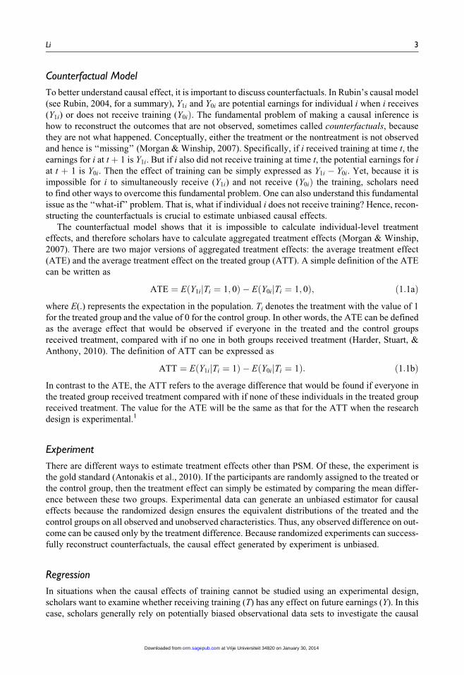
To better understand causal effect, it is important to discuss counterfactuals. In Rubin’s causal model

(see Rubin, 2004, for a summary), Y1i and Y0i are potential earnings for individual i when i receives

(Y1i) or does not receive training (Y0iÞ. The fundamental problem of making a causal inference is

how to reconstruct the outcomes that are not observed, sometimes called counterfactuals, because

they are not what happened. Conceptually, either the treatment or the nontreatment is not observed

and hence is ‘‘missing’’ (Morgan & Winship, 2007). Specifically, if i received training at time t, the

earnings for i at tþ 1 is Y1i. But if i also did not receive training at time t, the potential earnings for i

at t þ 1 is Y0i. Then the effect of training can be simply expressed as Y1i � Y0i. Yet, because it is

impossible for i to simultaneously receive (Y1i) and not receive (Y0iÞ the training, scholars need

to find other ways to overcome this fundamental problem. One can also understand this fundamental

issue as the ‘‘what-if’’ problem. That is, what if individual i does not receive training? Hence, recon-

structing the counterfactuals is crucial to estimate unbiased causal effects.

The counterfactual model shows that it is impossible to calculate individual-level treatment

effects, and therefore scholars have to calculate aggregated treatment effects (Morgan & Winship,

2007). There are two major versions of aggregated treatment effects: the average treatment effect

(ATE) and the average treatment effect on the treated group (ATT). A simple definition of the ATE

can be written as

ATE ¼ E Y1ijTi ¼ 1; 0ð Þ � EðY0ijTi ¼ 1; 0Þ; ð1:1aÞ

where E(.) represents the expectation in the population. Ti denotes the treatment with the value of 1

for the treated group and the value of 0 for the control group. In other words, the ATE can be defined

as the average effect that would be observed if everyone in the treated and the control groups

received treatment, compared with if no one in both groups received treatment (Harder, Stuart, &

Anthony, 2010). The definition of ATT can be expressed as

ATT ¼ E Y1ijTi ¼ 1ð Þ � EðY0ijTi ¼ 1Þ: ð1:1bÞ

In contrast to the ATE, the ATT refers to the average difference that would be found if everyone in

the treated group received treatment compared with if none of these individuals in the treated group

received treatment. The value for the ATE will be the same as that for the ATT when the research

design is experimental.1

Experiment

There are different ways to estimate treatment effects other than PSM. Of these, the experiment is

the gold standard (Antonakis et al., 2010). If the participants are randomly assigned to the treated or

the control group, then the treatment effect can simply be estimated by comparing the mean differ-

ence between these two groups. Experimental data can generate an unbiased estimator for causal

effects because the randomized design ensures the equivalent distributions of the treated and the

control groups on all observed and unobserved characteristics. Thus, any observed difference on out-

come can be caused only by the treatment difference. Because randomized experiments can success-

fully reconstruct counterfactuals, the causal effect generated by experiment is unbiased.

Regression

In situations when the causal effects of training cannot be studied using an experimental design,

scholars want to examine whether receiving training (T) has any effect on future earnings (Y). In this

case, scholars generally rely on potentially biased observational data sets to investigate the causal

Li 3




effect. For example, one can use a simple regression model by regressing future earnings (Y) on

training (T) and demographic variables such as age (x1) and race (x2).

Y ¼ b0 þ b1x1 þ b2x2 þ tT þ e: ð1:2Þ

Scholars then interpret the results by saying ‘‘ceteris paribus, the effect due to training is t.’’ They

typically assume t is the causal effect due to management intervention. Indeed, regression or the

structural equation models (SEM) (cf. Duncan, 1975; James, Mulaik, & Brett, 1982) is still a domi-

nant approach for estimating treatment effect.2 Yet, regression cannot detect whether the cases are

comparable in terms of distribution overlap on observed characteristics. Thus, regression models are

unable to reconstruct counterfactuals. One can easily find many empirical studies that seek to esti-

mate causal effects by regressing an outcome variable on an intervention dummy variable. The find-

ings of these studies, which used observational data sets, could be wrong because they did not adjust

for the distribution between the treated and control groups.

Endogeneity

In addition to the nonequivalence of distribution between the control and treated groups, another

severe error that prevents scholars from calculating unbiased causal effects is endogeneity. This

occurs when predictor T correlates with error term e in Equation 1.2. A number of review articles

have described the endogeneity problem and warned management scholars of its biasing effects

(e.g., Antonakis et al., 2010; Hamilton & Nickerson, 2003). As discussed previously, endogeneity

manifests from measurement error, simultaneity, and omitted variables. Measurement error

typically attenuates the effect size of regression estimators in explanatory variables. Simultaneity

happens when at least one of the predictors is determined simultaneously along with the dependent

variable. An example of simultaneity is the estimation of price in a supply and demand model

(Greene, 2008). An omitted variable appears when one does not control for additional variables that

correlate with explanatory as well as dependent variables.

Of these three sources of endogeneity, the omitted variable bias has probably received the most

attention from management scholars. Returning to the earlier training example, suppose the

researcher only controls for demographic variables but does not control for an individual’s ability.

If training correlates with ability and ability correlates with future earnings, the result will be biased

because of endogeneity. Consequently, omitting ability will cause a correlation between training

dummy T and residuals e. This violates the assumption of strict exogeneity for linear regression

models. Thus, the estimated causal effect (tÞ in Equation 1.2 will be biased. If the omitted variable

is time-invariant, one can use the fixed effects model to deal with endogeneity (Allison, 2009). Beck,

Bruderl, and Woywode’s (2008) simulation showed that the fixed effects model provided correction

for biased estimation due to the omitted variable.

One can also view nonrandom sample selection as a special case of the omitted variable problem.

Taking the effect of training on earnings as an example, one can only observe earnings for individ-

uals who are employed. Employed individuals could be a nonrandom subset of the population. One

can write the nonrandom selection process as Equation 1.3,

D ¼ aZ þ u; ð1:3Þ

where D is latent selection variable (1 for employed individuals), Z represents a vector of variables

(e.g., education level) that predicts selection, and u denotes disturbances. One can call Equation 1.2

the substantive equation and Equation 1.3 the selection equation. Sample selection bias is likely to

materialize when there is correlation between the disturbances for substantive (e) and selection

equation (u) (Antonakis et al., 2010, p. 1094; Berk, 1983; Heckman, 1979). When there is a correla-

tion between e and u, the Heckman selection model, rather than the PSM, should be used to calculate





causal effect (Antonakis et al., 2010). To correct for the sample selection bias, one can first fit the

selection model using probit or logit model. Then the predicted values from the selection model will

be saved to compute the density and distribution values, from which the inverse Mills ratio (l)—the

ratio for the density value to the distribution value—will be calculated. Finally, the inverse Mills

ratio will be included in the substantive Equation 1.2 to correct for the bias of t due to selection.

For more information on two-stage selection models, readers can consult Berk (1983).

The Propensity Score Method

Having briefly reviewed existing techniques for estimating causal effects, I now discuss how PSM

can help scholars to draw correct causal inferences. The PSM is a technique that allows researchers

to reconstruct counterfactuals using observational data. It does this by reducing two sources of bias

in the observational data: bias due to lack of distribution overlap and bias due to different density

weighting (Heckman, Ichimura, Smith, & Todd, 1998). A propensity score can be defined as the

probability of study participants receiving a treatment based on observed characteristics. The PSM

refers to a special procedure that uses propensity scores and matching algorithm to calculate the cau-

sal effect.

Before moving on, it is useful to conceptually differentiate PSM from Heckman’s (1979) ‘‘selec-

tion model.’’ His selection model deals with the probability of treatment assignment indirectly from

instrumental variables. Thus, the probability calculated using the selection model requires one or

more variables that are not censored or truncated and that can predict the selection. For example,

if one wanted to study how training affects future earnings, one must consider the self-selection

problem, because wages can only be observed for individuals who are already employed. Using the

predicted probability calculated from the first stage (Equation 1.3), one can compute the inverse

Mills ratio and insert this variable to the wage prediction model to correct for selection bias. In con-

trast to the predicted probability calculated in the Heckman selection model, propensity scores are

calculated directly only through observed predictors. Furthermore, the propensity scores and the pre-

dicted probabilities calculated using Heckman selection have different purposes in estimating causal

effects: The probabilities estimated from the Heckman model generate an inverse Mills ratio that can

be used to adjust for bias due to censoring or truncation, whereas the probabilities calculated in the

PSM are used to adjust covariate distribution between the treated group and the control group.

Reasons for Using the PSM

Because there are many methods that can estimate causal effects, why should management scholars

care about the PSM? One reason is that most publications in the management field rely on observa-

tional data. Such large data can be relatively inexpensive to obtain, yet they are almost always obser-

vational rather than experimental. By adjusting covariates between the treated and control groups,

the PSM allows scholars to reconstruct counterfactuals using observational data. If the strongly

ignorable assumption that will be discussed in the next section is satisfied, then the PSM can produce

an unbiased causal effect using observational data sets.

Second, mis-specified econometric models using observational data sometimes produce biased

estimators. One source of such bias is that the two samples lack distribution overlap, and regression

analysis cannot tell researchers the distribution overlap between two samples. Cochran (1957, pp.

265-266) illustrated this problem using the following example: ‘‘Suppose that we were adjusting for

differences in parents’ income in a comparison of private and public school children, and that the

private-school incomes ranged from $10,000–$12,000, while the public-school incomes ranged

from $4,000–$6,000. The covariance would adjust results so that they allegedly applied to a mean

income of $8,000 in each group, although neither group has any observations in which incomes are

Li 5




at or near this level.’’ The PSM can easily detect the lack of covariate distribution between two

groups and adjust the distribution accordingly.

Third, linear or logistic models have been used to adjust for confounding covariates, but such

models rely on assumptions regarding functional form. For example, one assumption required for

a linear model to produce an unbiased estimator is that it does not suffer from the aforementioned

problem of endogeneity. Although the procedure to calculate propensity scores is parametric, using

propensity scores to compute causal effect is largely nonparametric. Thus, using the PSM to calcu-

late the causal effect is less susceptible to the violation of model assumptions. Overall, when one is

interested in investigating the effectiveness of a certain management practice but is unable to collect

experimental data, the PSM should be used, at least as a robust test to justify the findings estimated

by parametric models.

Overview of the PSM

The concept of subclassification is helpful for understanding the PSM. Simply comparing the mean

difference of the outcome variables in two groups typically leads to biased estimators, because the

distributions of the observational variables in the two groups may differ. Cochran’s (1968) subclas-

sification method first divides an observational variable into n subclasses and then estimates the

treatment effect by comparing the weighted means of the outcome variable in each subclass. He used

two approaches to demonstrate the effectiveness of subclassification in reducing bias in observa-

tional studies. First, he used an empirical example (death rate for smoking groups with country of

origin and age as covariates) to show that when age was divided into two classes more than half the

effect of the age bias was removed. Second, he used a mathematical model to derive the proportion

of bias that can be removed through subclassification. For different distribution functions, using five

or six subclasses will typically remove 90% or more of the bias shown in the raw comparison. With

more than six subclasses, only small amounts of additional bias can be removed. Yet, subclassifica-

tion is difficult to utilize if many confounding covariates exist (Rubin, 1997).

To overcome the difficulty of estimating the treatment effects using Cochran’s technique, Rosen-

baum and Rubin (1983) developed the PSM. The key objective of the PSM is to replace the many

confounding covariates in an observational study with one function of these covariates. The function

(or the propensity score) captures the likelihood of study participants receiving a treatment based on

observed covariates. The estimated propensity score is then used as the only confounding covariate

to adjust for all of the covariates that go into the estimation. Since the propensity score adjusts for all

covariates using a simple variable and Cochran found that five blocks can remove 90% of bias due to

raw comparison, stratifying the propensity score into five blocks can generally remove much of the

difference due to the non-overlap of all observed covariates between the treated group and the con-

trol group.

Central to understanding the PSM is the balancing score. Rosenbaum and Rubin (1983) defined

the balancing score as a function of observable covariates such that the conditional distribution of X

given the balancing score is the same for the treated group and the control group. Formally, the bal-

ancing score bðX Þ satisfies X?T jbðX Þ, where X is a vector of the observed covariates, T represents

the treatment assignment, and? refers to independence. Rosenbaum and Rubin argued that the pro-

pensity score is a type of balancing score. They further proved that the finest balancing score is

b Xð Þ ¼ X , the coarsest balancing score is the propensity score, and any score that is finer than the

propensity score is the balancing score.

Rosenbaum and Rubin (1983) also introduced the strongly ignorable assumption, which implies

that given the balancing scores, the distributions of the covariates between the treated and the control

groups are the same. They further showed that treatment assignment is strongly ignorable if it satis-

fies the condition of unconfoundedness and overlap. Unconfoundedness means that conditional on





observational covariates X, potential outcomes (Y1 and Y0) are not influenced by treatment assign-

ment (Y1; Y0?T jX ). This assumption simply asserts that the researcher can observe all variables that

need to be adjusted. The overlap assumption means that given covariates X, the person with the same

X values has positive and equal opportunity of being assigned to the treated group or the control

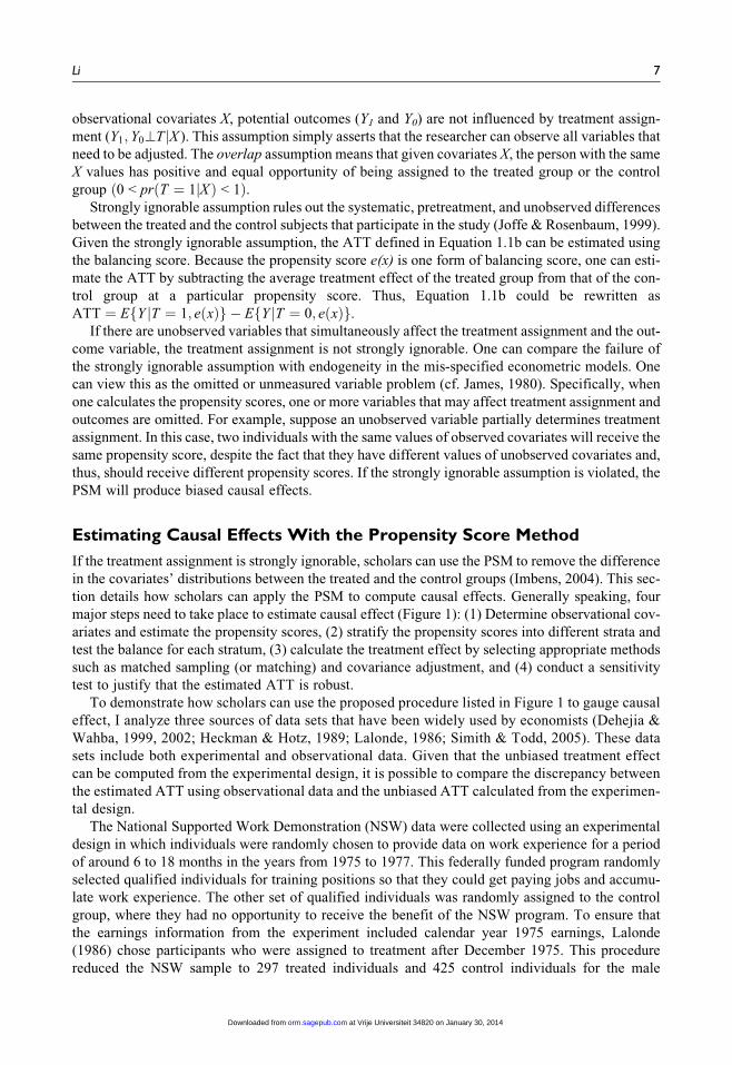
group ð0 < pr T ¼ 1jXð Þ < 1Þ.Strongly ignorable assumption rules out the systematic, pretreatment, and unobserved differences

between the treated and the control subjects that participate in the study (Joffe & Rosenbaum, 1999).

Given the strongly ignorable assumption, the ATT defined in Equation 1.1b can be estimated using

the balancing score. Because the propensity score e(x) is one form of balancing score, one can esti-

mate the ATT by subtracting the average treatment effect of the treated group from that of the con-

trol group at a particular propensity score. Thus, Equation 1.1b could be rewritten as

ATT ¼ EfY jT ¼ 1; e xð Þg � EfY jT ¼ 0; e xð Þg.If there are unobserved variables that simultaneously affect the treatment assignment and the out-

come variable, the treatment assignment is not strongly ignorable. One can compare the failure of

the strongly ignorable assumption with endogeneity in the mis-specified econometric models. One

can view this as the omitted or unmeasured variable problem (cf. James, 1980). Specifically, when

one calculates the propensity scores, one or more variables that may affect treatment assignment and

outcomes are omitted. For example, suppose an unobserved variable partially determines treatment

assignment. In this case, two individuals with the same values of observed covariates will receive the

same propensity score, despite the fact that they have different values of unobserved covariates and,

thus, should receive different propensity scores. If the strongly ignorable assumption is violated, the

PSM will produce biased causal effects.

Estimating Causal Effects With the Propensity Score Method

If the treatment assignment is strongly ignorable, scholars can use the PSM to remove the difference

in the covariates’ distributions between the treated and the control groups (Imbens, 2004). This sec-

tion details how scholars can apply the PSM to compute causal effects. Generally speaking, four

major steps need to take place to estimate causal effect (Figure 1): (1) Determine observational cov-

ariates and estimate the propensity scores, (2) stratify the propensity scores into different strata and

test the balance for each stratum, (3) calculate the treatment effect by selecting appropriate methods

such as matched sampling (or matching) and covariance adjustment, and (4) conduct a sensitivity

test to justify that the estimated ATT is robust.

To demonstrate how scholars can use the proposed procedure listed in Figure 1 to gauge causal

effect, I analyze three sources of data sets that have been widely used by economists (Dehejia &

Wahba, 1999, 2002; Heckman & Hotz, 1989; Lalonde, 1986; Simith & Todd, 2005). These data

sets include both experimental and observational data. Given that the unbiased treatment effect

can be computed from the experimental design, it is possible to compare the discrepancy between

the estimated ATT using observational data and the unbiased ATT calculated from the experimen-

tal design.

The National Supported Work Demonstration (NSW) data were collected using an experimental

design in which individuals were randomly chosen to provide data on work experience for a period

of around 6 to 18 months in the years from 1975 to 1977. This federally funded program randomly

selected qualified individuals for training positions so that they could get paying jobs and accumu-

late work experience. The other set of qualified individuals was randomly assigned to the control

group, where they had no opportunity to receive the benefit of the NSW program. To ensure that

the earnings information from the experiment included calendar year 1975 earnings, Lalonde

(1986) chose participants who were assigned to treatment after December 1975. This procedure

reduced the NSW sample to 297 treated individuals and 425 control individuals for the male

Li 7




participants. Dehejia and Wahba (1999, 2002) reconstructed Lalonde’s original NSW data by

including individuals who attended the program early enough to obtain retrospective 1974 earning

information. The final NSW sample includes 185 treated and 265 control individuals.

Lalonde’s (1986) observational data consisted of two distinct comparison groups in the years

between 1975 and 1979: the Population Survey of Income Dynamics (PSID-1) and the Current Pop-

ulation Survey–Social Security Administration File (CPS-1). Initiated in 1968, the PSID is a nation-

ally representative longitudinal database that interviewed individuals and families for information

on dynamics of employment, income, and earnings. The CPS, a monthly survey conducted by

Bureau of the Census for the Bureau of Labor Statistics, provides comprehensive information on the

unemployment, income, and poverty of the nation’s population. Lalonde further extracted four data

sets (denoted as PSID-2, PSID-3, CPS-2, and CPS-3) that represent the treatment group based on

Step 1: estimating propensity score

Estimate PScore: 1. Logit/probit 2. Ordinal probit 3. Multinomial logit 4. Hazard

High-order covariates

Stratify PScore to different strata Step 2: stratifying and

balancing propensity score

Covariate is not balanced

Test for balance of covariate

Covariate is balanced

Estimate causal effect:

1. Matched sampling 1) Stratified matching 2) Nearest neighbor matching 3) Radius matching 4) Kernel matching

2. Covariate adjustment

Step 3: estimating causal effect

Sensitivity test: 1. Multiple comparison groups2. Specification3. Instrumental variables4. Rosenbaum bounds

Step 4: sensitivity test

Determine observational

covariates

Figure 1. Steps for estimating treatment effectsNote: PScore ¼ propensity scores.





simple pre-intervention characteristics (e.g., age or employment status; see Table 1a for details).

Table 1a reports details of data sets and the definitions of the variables.

Step 1: Estimating the Propensity Scores

To calculate a propensity score, one first needs to determine the covariates. Heckman, Ichimura, and

Todd (1997) demonstrated that the quality of the observational variables has a significant impact on

the estimated results. Having knowledge of relevant theory, institutional settings, and previous

research is beneficial for scholars to specify which variables should be included in the model (Simith

& Todd, 2005). To appropriately represent the theory, scholars need to specify not only the observa-

tional covariates but also the high-order covariates such as quadratic effects and interaction effects.

From a methodological perspective, researchers need to add high-order covariates to achieve strata

balance. The process of adding high-order covariates will be discussed in the section detailing how

to obtain a balance of propensity scores in each stratum. A recent development called boosted

regression can also be implemented to calculate propensity scores (McCaffrey, Ridgeway, &

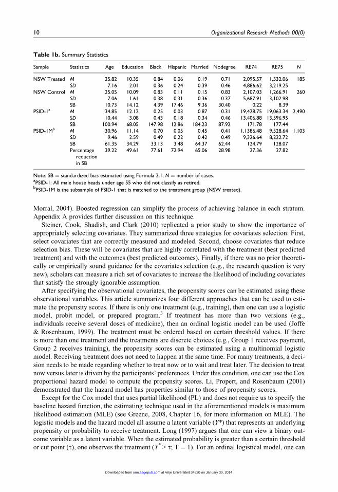
Table 1a. Description of Data Sets and Definition of Variables

Data Sets Sample Size Description

NSW Treated 185 National Supported Work Demonstration (NSW) data werecollected using experimental design, where qualified individualswere randomly assigned to the training position to receive payand accumulate experience.

NSW Control 260 Experimental control group: The set of qualified individuals wererandomly assigned to this control group so that they have noopportunity to receive the benefit of NSW program.

PSID-1 2,490 Nonexperimental control group: 1975-1979 Population Survey ofIncome Dynamics (PSID) where all male household heads underage 55 who did not classify as retired in 1975.

PSID-2 253 Data set was selected from PSID-1 who were not working in thespring of 1976.

PSID-3 128 Data set was selected from PSID-2 who were not working in thespring of 1975.

CPS-1 15,992 Nonexperimental control group: 1975-1979 Current PopulationSurvey (CPS) where all participants with age under 55.

CPS-2 2,369 Data set was selected from CPS-1 where all men who were notworking when surveyed in March 1976.

CPS-3 429 Data set was selected from CPS-2 where all unemployed men in1976 whose income in 1975 was below the poverty line.

Variables Definition

Treatment Set to 1 if the participant comes from NSW treated data set, 0otherwise

Age The age of the participants (in years)Education Number of years of schoolingBlack Set to 1 for Black participants, 0 otherwiseHispanic Set to 1 for Hispanic participants, 0 otherwiseMarried Set to 1 for married participants, 0 otherwiseNodegree Set to 1 for the participants with no high school degree, 0 otherwiseRE74 Earnings in 1974RE75 Earnings in 1975RE78 Earnings in 1978, the outcome variable

Li 9




Morral, 2004). Boosted regression can simplify the process of achieving balance in each stratum.

Appendix A provides further discussion on this technique.

Steiner, Cook, Shadish, and Clark (2010) replicated a prior study to show the importance of

appropriately selecting covariates. They summarized three strategies for covariates selection: First,

select covariates that are correctly measured and modeled. Second, choose covariates that reduce

selection bias. These will be covariates that are highly correlated with the treatment (best predicted

treatment) and with the outcomes (best predicted outcomes). Finally, if there was no prior theoreti-

cally or empirically sound guidance for the covariates selection (e.g., the research question is very

new), scholars can measure a rich set of covariates to increase the likelihood of including covariates

that satisfy the strongly ignorable assumption.

After specifying the observational covariates, the propensity scores can be estimated using these

observational variables. This article summarizes four different approaches that can be used to esti-

mate the propensity scores. If there is only one treatment (e.g., training), then one can use a logistic

model, probit model, or prepared program.3 If treatment has more than two versions (e.g.,

individuals receive several doses of medicine), then an ordinal logistic model can be used (Joffe

& Rosenbaum, 1999). The treatment must be ordered based on certain threshold values. If there

is more than one treatment and the treatments are discrete choices (e.g., Group 1 receives payment,

Group 2 receives training), the propensity scores can be estimated using a multinomial logistic

model. Receiving treatment does not need to happen at the same time. For many treatments, a deci-

sion needs to be made regarding whether to treat now or to wait and treat later. The decision to treat

now versus later is driven by the participants’ preferences. Under this condition, one can use the Cox

proportional hazard model to compute the propensity scores. Li, Propert, and Rosenbaum (2001)

demonstrated that the hazard model has properties similar to those of propensity scores.

Except for the Cox model that uses partial likelihood (PL) and does not require us to specify the

baseline hazard function, the estimating technique used in the aforementioned models is maximum

likelihood estimation (MLE) (see Greene, 2008, Chapter 16, for more information on MLE). The

logistic models and the hazard model all assume a latent variable (Y*) that represents an underlying

propensity or probability to receive treatment. Long (1997) argues that one can view a binary out-

come variable as a latent variable. When the estimated probability is greater than a certain threshold

or cut point (t), one observes the treatment (Y* > t; T ¼ 1). For an ordinal logistical model, one can

Table 1b. Summary Statistics

Sample Statistics Age Education Black Hispanic Married Nodegree RE74 RE75 N

NSW Treated M 25.82 10.35 0.84 0.06 0.19 0.71 2,095.57 1,532.06 185SD 7.16 2.01 0.36 0.24 0.39 0.46 4,886.62 3,219.25

NSW Control M 25.05 10.09 0.83 0.11 0.15 0.83 2,107.03 1,266.91 260SD 7.06 1.61 0.38 0.31 0.36 0.37 5,687.91 3,102.98SB 10.73 14.12 4.39 17.46 9.36 30.40 0.22 8.39

PSID-1a M 34.85 12.12 0.25 0.03 0.87 0.31 19,428.75 19,063.34 2,490SD 10.44 3.08 0.43 0.18 0.34 0.46 13,406.88 13,596.95SB 100.94 68.05 147.98 12.86 184.23 87.92 171.78 177.44

PSID-1Mb M 30.96 11.14 0.70 0.05 0.45 0.41 1,1386.48 9,528.64 1,103SD 9.46 2.59 0.49 0.22 0.42 0.49 9,326.64 8,222.72SB 61.35 34.29 33.13 3.48 64.37 62.44 124.79 128.07Percentage

reductionin SB

39.22 49.61 77.61 72.94 65.06 28.98 27.36 27.82

Note: SB ¼ standardized bias estimated using Formula 2.1; N ¼ number of cases.aPSID-1: All male house heads under age 55 who did not classify as retired.

bPSID-1M is the subsample of PSID-1 that is matched to the treatment group (NSW treated).





understand the latent variable with multiple thresholds and observe the treatment according to the

thresholds (e.g., t1 < Y* < t2; T ¼ 2). The multinomial logistical model can simply be viewed as

the model that simultaneously estimates a binary model for all possible comparisons among outcome

categories (Long, 1997), but it is more efficient to use a multinomial logistical model than using

multiple binary models. It is somewhat tricky to generate the predicted probability from the Cox

model because it is semiparametric with no assumption of the distribution of baseline. Two alterna-

tive choices can be used to better derive probability for survival model: (1) One can rely on a para-

metric survival model that specifies the baseline model; (2) one can transform the data in order to use

the discrete-time model.

To illustrate how to calculate propensity scores, this study employed treatment group data from

the NSW and control group data from the observational data extracted from the PSID-2. Following

Dehejia and Wahba (1999), I selected age, education, no degree, Black, Hispanic, RE74, RE75, age

square, RE74 square, RE75 square, and RE74 � Black as covariates to calculate propensity scores.

To compute propensity scores, one can first run a logistic or probit model using a treatment

dummy (whether an individual received training) as the dependent variable and the aforemen-

tioned covariates as the independent variables. Propensity scores can be obtained by calculating

the fitted value from the logistic or probit models (use –predict mypscore, p– in STATA). Readers

can refer Hoetker (2007) for more information on calculating probability from logit or probit mod-

els. After calculating propensity scores, Appendix B includes a randomly selected sample (n¼ 50)

from the combined data set NSW and PSID-2. Readers can obtain data for Appendix B, NSW

treated, and PSID-2 from the author.

Step 2: Stratifying and Balancing the Propensity Scores

After estimating the propensity scores, the next step is to subclassify them into different strata such

that these blocks are balanced on propensity scores. The number of balanced propensity score blocks

depends on the number of observations in the data set. As discussed previously, five blocks are a good

starting point to stratify the propensity scores (Rosenbaum & Rubin, 1983). One then can test the bal-

ance of each block by examining the distribution of covariates and the variance of propensity scores.

The t test and the test for standardized bias (SB) are two widely used techniques to ensure the balance

of the strata (Rosenbaum & Rubin, 1985). The t-test compares whether the means of covariates differ

between the treated and the matched control groups. The SB approach calculates the difference of sam-

ple means in the treated and the matched control groups as a percentage of the square root of the aver-

age sample variance in both groups. To conduct the SB test, scholars need to compare values

calculated before and after matching. The formula used to calculate the SB value can be written as

SBmatch ¼ 100j �X1M � �X0M jffiffiffiffiffiffiffiffiffiffiffiffiffiffiffiffiffiffiffiffiffiffiffiffiffiffiffiffiffiffiffiffiffiffiffiffiffiffiffiffiffiffiffiffiffi

0:5ðV1M Xð Þ þ V0M ðX Þp

Þ; ð2:1Þ

where �X1M ðV1M Þ and �X0MðV0MÞ are the means (variance) for the treated group and the matched con-

trol group. In addition to these two widely used tests, the Kolmogorov-Smirnov’s two-sample test can

also be used to investigate the overlap of the covariates between the treated and the control groups.

Balanced strata between the treated and the matched control group ensure the minimal distance in

the marginal distributions of the covariates. If any pretreatment variable is not balanced in a partic-

ular block, one needs to subclassify the block into additional blocks until all blocks are balanced. To

obtain strata balance, researchers sometimes need to add high-order covariates and recalculate the

propensity scores. Rosenbaum and Rubin (1984) detailed the process of cycling between checking

for balance within strata and reformulating the propensity model. Two guidelines for adding

high-order covariates have been proposed: (1) When the variances of a critical covariate are found

Li 11




to differ dramatically between the treatment and the control group, the squared terms of the covariate

need to be included in the revised propensity score model and (2) when the correlation between two

important covariates differs greatly between the groups, the interaction of the covariates can be

added to the propensity score model.

Appendix B shows a simple example of stratifying data into five blocks after calculating the pro-

pensity scores. For this illustration, I stratified the 50 cases into five groups. I first identified the

cases with propensity scores smaller than 0.05, which were classified as unmatched. When the pro-

pensity scores were smaller than 0.2 but larger than 0.05, I coded this as block 1 (Block ID ¼ 1).

When the propensity scores were smaller than 0.4 but larger than 0.2, this was coded as block 2. This

process was repeated until I had created five blocks, and then I conducted the t-test within each block

to detect any significant difference of propensity scores between the treated and control groups. T-

values for each block were added in the columns next to the column of Block ID. Overall, the t-test

reveals that the difference of propensity scores between the treated and control groups is statistically

insignificant. If the t-test shows that there are statistically significant differences in propensity

scores, one should either change threshold value of propensity scores in each block or change the

covariates to recalculate the propensity scores.

When the propensity scores in each stratum are balanced, all covariates in each stratum should

also achieve equivalence of distribution. To confirm this, one can conduct the t-test for each obser-

vational variable. To illustrate how balance of propensity scores within strata helps to achieve dis-

tribution overlap for other covariates, Appendix B reports the values for one continuous variable,

age. One can conduct the t-test to ensure that there is no age difference between the treated and con-

trol groups within each stratum. The column Tage reports the t-test for age within the strata. After

balancing each block’s propensity scores, the age difference between the treated and control groups

in each block became statistically insignificant. I recommend that readers use a prepared statistic

package to stratify propensity scores, as a program can simultaneously categorize propensity scores

and conduct balance tests. For instance, one can use the -pscore- program in STATA (Becker &

Ichino, 2002) to estimate, stratify, and test the balance of propensity scores.

To further illustrate how the PSM can achieve strata balance, I replicated the aforementioned two

procedures for the combined experimental data set and each of the observational data sets in Table

1a. Following Dehejia and Wahba’s (1999) suggestions on choice of covariates, I first computed

propensity scores for each data set. Then, the propensity scores were stratified and tested for the bal-

ance within each stratum. When the propensity scores achieved balance within each stratum, I

plotted the means of propensity scores in each stratum for each matched data set. Figure 2 provides

evidence that the means of the propensity scores are almost the same for each sample within each

balanced block.

To demonstrate the effectiveness of the PSM in adjusting for the balance of other covariates,

Table 1b summarizes the means, standard errors, and SB of the matched sample. Comparing the

results between the matched and unmatched samples, one can see that the difference of most

observed characteristics between the experimental design and the nonexperimental design reduces

dramatically. For instance, PSID-1 of Table 1b reports that the absolute SB values range from 12.86

to 184.23 (before using propensity score matching), but PSID-1M of Table 1b shows that the abso-

lute minimum value of SB is 3.48 and the absolute maximum value of SB is 128.07.

Furthermore, the t-test and the Kolmogorov-Smirnov sample test were conducted to examine the

balance of each variable. As reported from Table 2, for the PSID-1 sample, except for RE74 in Block

3, one cannot see a p value smaller than 0.1. For simplicity, Table 2 uses only continuous variables

that have been included for estimating the propensity scores to illustrate the effectiveness of the PSM

in increasing the distribution overlap between the treated group and the matched control group.

Overall, Table 2 shows strong evidence that after obtaining balance of propensity scores within a

stratum, the covariates achieve overlap in terms of distribution. To preserve space, Table 1b and





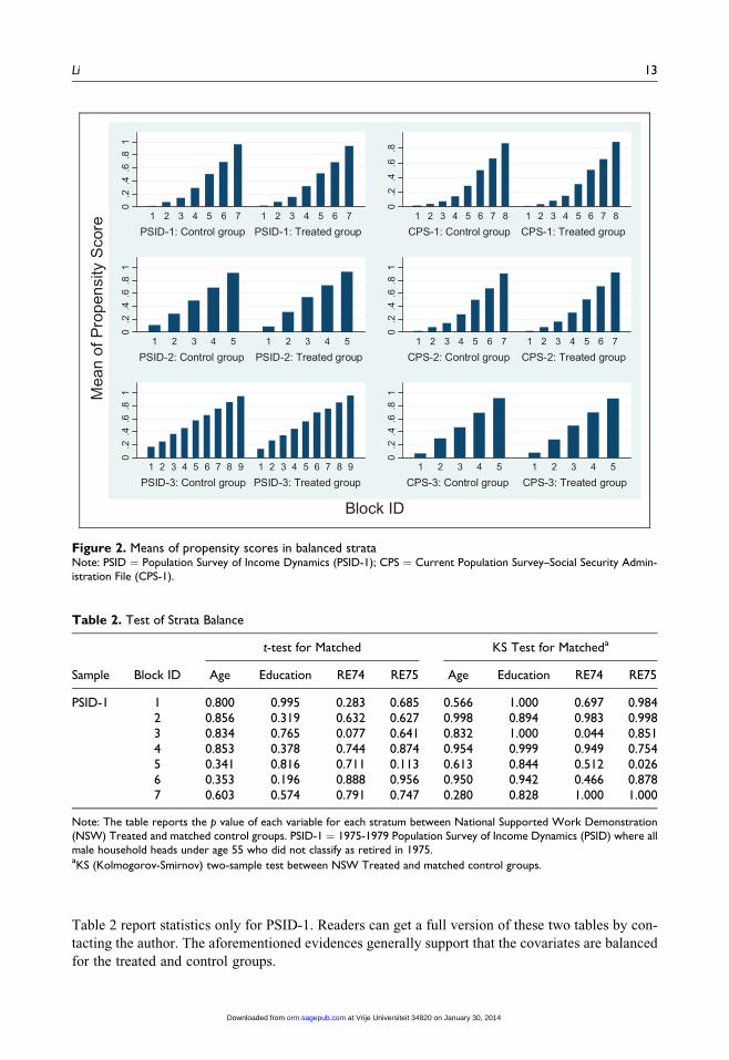
Table 2 report statistics only for PSID-1. Readers can get a full version of these two tables by con-

tacting the author. The aforementioned evidences generally support that the covariates are balanced

for the treated and control groups.

Table 2. Test of Strata Balance

Sample Block ID

t-test for Matched KS Test for Matcheda

Age Education RE74 RE75 Age Education RE74 RE75

PSID-1 1 0.800 0.995 0.283 0.685 0.566 1.000 0.697 0.9842 0.856 0.319 0.632 0.627 0.998 0.894 0.983 0.9983 0.834 0.765 0.077 0.641 0.832 1.000 0.044 0.8514 0.853 0.378 0.744 0.874 0.954 0.999 0.949 0.7545 0.341 0.816 0.711 0.113 0.613 0.844 0.512 0.0266 0.353 0.196 0.888 0.956 0.950 0.942 0.466 0.8787 0.603 0.574 0.791 0.747 0.280 0.828 1.000 1.000

Note: The table reports the p value of each variable for each stratum between National Supported Work Demonstration(NSW) Treated and matched control groups. PSID-1 ¼ 1975-1979 Population Survey of Income Dynamics (PSID) where allmale household heads under age 55 who did not classify as retired in 1975.aKS (Kolmogorov-Smirnov) two-sample test between NSW Treated and matched control groups.

0.2

.4.6

.81

PSID-1: Control group PSID-1: Treated group1 2 3 4 5 6 7 1 2 3 4 5 6 7

0.2

.4.6

.8

CPS-1: Control group CPS-1: Treated group1 2 3 4 5 6 7 8 1 2 3 4 5 6 7 8

0.2

.4.6

.81

PSID-2: Control group PSID-2: Treated group1 2 3 4 5 1 2 3 4 5

0.2

.4.6

.81

CPS-2: Control group CPS-2: Treated group1 2 3 4 5 6 7 1 2 3 4 5 6 7

0.2

.4.6

.81

PSID-3: Control group PSID-3: Treated group1 2 3 4 5 6 7 8 9 1 2 3 4 5 6 7 8 9

0.2

.4.6

.81

CPS-3: Control group CPS-3: Treated group1 2 3 4 5 1 2 3 4 5

Mea

n of

Pro

pens

ity S

core

Block ID

Figure 2. Means of propensity scores in balanced strataNote: PSID ¼ Population Survey of Income Dynamics (PSID-1); CPS ¼ Current Population Survey–Social Security Admin-istration File (CPS-1).

Li 13




Step 3: Estimating the Causal Effect

Because the data sets include an experimental design, one can compute the unbiased causal effect.

Table 3 shows the estimated results of training on earnings in 1978 (RE78). The first row of Table 3

reports the benchmark values calculated using the experimental data. The unadjusted result

($1,794.34) was calculated by subtracting the mean of RE78 in the treated group (NSW Treated)

from the mean of RE78 in the control group (NSW Control). The adjusted estimation ($1,676.34)

was computed by using regression, controlling for all observational covariates. Because the experi-

mental data compiled by Lalonde (1986) does not achieve the same distribution between the treated

and control groups (Table 1b), this article uses the causal effect value calculated by the adjusted esti-

mation as the benchmark value. From Table 3 column 1, it is obvious that if there are substantial

differences among the pretreatment variables (as shown in Table 1b), using the mean difference

to estimate the causal effect is strongly biased (it ranges from –$15,204.78 to $1,069.85). In Table

3 column 2, a simple linear regression model was used to gauge the adjusted training effects. Col-

umn 2 shows that the estimated treatment effects (with a range from $699.13 to $1,873.77) are more

reliable than those calculated using the mean differences.

In addition to mean difference and regression, PSM can also be used to effectively estimate the

ATT. When the propensity scores are balanced in all strata, one can use two standard techniques to

compute the ATT: matched sampling (e.g., stratified matching, nearest neighbor matching, radius

matching, and kernel matching) and covariance adjustment. Matched sampling or matching is a

technique used to sample certain covariates from the treated group and the control group to obtain

a sample with similar distributions of covariates between the two groups.4 Rosenbaum (2004) con-

cluded that propensity score matching can increase the robustness of the model-based adjustment

and avoid unnecessarily detailed description. The quality of the matched samples depends on the

covariate balance and the structure of the matched sets (Gu & Rosenbaum, 1993).

Ideally, exact matching on all confounding variables is the best matching approach because the

sample distribution of all confounding variables would be identical in the treated and control groups.

Unfortunately, exact matching on a single confounding variable will reduce the number of final

matched cases. Supposing that there are k confounding variables and each variable has three levels,

there will be 3k patterns of levels to get perfectly matched samples. Thus, it is impractical to use the

exact matching technique to get the identical distribution of confounding variables between the two

groups. The PSM is more appropriate than exact matching because it reduces the covariates from

k-dimensional to one-dimensional. Rosenbaum and Rubin (1983) also showed that the PSM not only

simplified the matching algorithm, but also increased the quality of the matches.

Stratified Matching

After achieving strata balance, one can apply stratified matching to calculate the ATT. In each

balanced block, the average differences in the outcomes of the treated group and the matched control

group are calculated. The ATT will be estimated by the mean difference weighted by the number of

treated cases in each block. The ATT can be expressed as

ATT ¼XQ

q¼1

ðP

i2I qð Þ YTi

NTq

�P

j2I qð Þ YCj

NCq

Þ �NT

q

NT; ð2:2Þ

where Q denotes the number of blocks with balanced propensity scores, NTq and NC

q refer to the num-

ber of cases in the treated and the control groups for matched block q, Y Ti andY C

j represent the obser-

vational outcomes for case i in the matched treated group q and case j in the matched control group q,

respectively, and NT stands for the total number of cases in the treated group.





Tab

le3.

Est

imat

ion

Res

ults AT

T

Mat

chin

g

Cova

riat

eA

dju

stm

ent

Stra

tifie

dN

eigh

bor

Rad

ius

Ker

nel

Unad

just

eda

Adju

sted

bA

TT

cN

dA

TT

Nd

AT

Te

Nd

AT

Tf

Nd

AT

Tg

Nd

12

34

56

78

910

11

12

NSW

1,7

94.3

41,6

76.3

4(6

38.6

8)

PSI

D-1

h–15,2

04.7

8751.9

51,6

37.4

31,2

88

1,6

54.5

7248

1,8

71.4

437

1,5

07.1

01153

1,9

52.2

31,2

88

(915.2

6)

(805.4

3)

(1,1

74.6

3)

(5,8

37.1

0)

(826.1

1)

(791.4

5)

PSI

D-2

h–3,6

46.8

11,8

73.7

71,4

67.0

4308

1,6

04.0

9231

1,5

19.6

077

1,7

12.1

8297

1,5

93.3

2308

(1,0

60.5

6)

(1,4

61.7

5)

(1,0

92.4

0)

(2,1

10.7

1)

(1,2

26.9

0)

(1,4

76.5

4)

PSI

D-3

h1,0

69.8

51,8

33.1

31,8

43.2

0250

1,5

22.2

3217

1,6

32.7

4167

1,7

76.3

7245

1,5

83.4

1250

(1,1

59.7

8)

(981.4

2)

(1,9

20.2

4)

(1,5

98.1

2)

(1,4

25.3

2)

(1,8

66.4

6)

CPS-

1i

–8,4

97.5

2699.1

31,4

88.2

94,5

63

1,6

00.7

4280

1,8

90.1

3102

1,5

13.7

84,1

44

1,6

34.8

14,5

63

(547.6

4)

(716.7

9)

(957.0

5)

(1,9

93.5

0)

(726.4

7)

(515.5

8)

CPS-

2i

–3,8

21.9

71,1

72.7

01,6

76.4

31,4

38

1,6

38.7

4271

1,7

75.9

979

1,5

90.4

91,4

16

1,5

50.9

01,4

38

(645.8

6)

(796.6

2)

(1,0

14.6

4)

(2,2

86.2

3)

(736.8

5)

(625.0

4)

CPS-

3i

–635.0

31,5

48.2

41,5

05.4

9508

1,3

76.6

5273

1,3

07.6

353

1,1

66.9

3493

1,5

72.0

9508

(781.2

8)

(1,0

65.5

2)

(1,1

29.2

4)

(2,8

21.5

6)

(864.3

8)

(943.6

5)

Mea

nj

–5,1

22.7

11,3

13.1

51,6

02.9

81,5

66.1

71,5

44.4

71,6

66.2

61,6

47.8

0V

aria

nce

j3,5

078,9

50.9

270,3

27.3

221,0

84.8

210,7

12.1

145,7

79.0

951,1

01.5

223,0

16.4

6

Note

:Boots

trap

with

100

replic

atio

ns

was

use

dto

estim

ate

stan

dar

der

rors

for

the

pro

pen

sity

score

mat

chin

g;st

andar

der

rors

inpar

enth

eses

.a T

he

mea

ndiff

eren

cebet

wee

ntr

eatm

ent

group

(NSW

Tre

ated

)an

dco

rres

pondin

gco

ntr

olgr

oups

(NSW

Contr

ol,

PSI

D-1

toC

SP-3

).bLe

ast

squar

esre

gres

sion:re

gres

sR

E78

(ear

nin

gin

1978)

on

age,

trea

tmen

tdum

my,

educa

tion,no

deg

ree,

Bla

ck,H

ispan

ic,R

E74

(ear

nin

gin

1974),

and

RE75

(ear

nin

gin

1975).

c Stra

tify

ing

blo

cks

bas

edon

prop

ensity

scor

es,an

dth

enuse

Form

ula

2.2

toes

tim

ate

AT

T(a

vera

getr

eatm

ent

effe

cton

trea

ted).

dT

he

tota

lnum

ber

ofobse

rvat

ions,

incl

udin

gobse

rvat

ions

inN

SWT

reat

edan

dco

rres

pondin

gm

atch

edco

ntr

olgr

oups.

eFo

rK

ernel

mat

chin

g,w

hen

the

num

ber

ofca

ses

issm

all,

use

nar

row

erban

dw

idth

(.01)

inst

ead

of.0

6.

f Rad

ius

valu

era

nge

sfr

om

.0001

to.0

000025.

g Use

regr

essi

on,ta

kew

eigh

ts,w

hic

har

edef

ined

by

the

num

ber

oftr

eate

dobse

rvat

ions

inea

chbal

ance

dpr

open

sity

scor

eblo

ck.

hO

bse

rvat

ional

cova

riat

es:ag

e,tr

eatm

ent

dum

my,

educa

tion,no

deg

ree,

Bla

ck,H

ispan

ic,R

E74,an

dR

E75.H

igher

ord

erco

vari

ates

:ag

e2,R

E74

2,R

E75

2,R

E74�

Bla

ck.

i Obse

rvat

ional

cova

riat

es:sa

me

ash;hig

h-o

rder

cova

riat

es:ag

e2,ed

uca

tion

2,R

E74

2,R

E75

2,Educa

tion�

RE74.

j Mea

nan

dva

rian

cear

eca

lcula

ted

usi

ng

estim

ated

AT

Tfo

rea

chte

chniq

ue.

15 at Vrije Universiteit 34820 on January 30, 2014orm.sagepub.comDownloaded from



After stratifying data into different blocks, one can calculate the ATT using data listed in Appen-

dix B. First, one can computeP

i2I 1ð ÞY T

i (the summation of the outcome variable in each block for each

of the treated cases, denoted as YiT in Appendix B) and

Pj2I 1ð Þ

Y Cj (the summation of the outcome vari-

able in each block for each of the control cases, denoted as YjC in Appendix B). For example, in

block 1 the summation of the outcome for two treated cases is 49,237.66, and the summation of the

outcome for five control cases is 31,301.69. The number of cases in the treatment (NT1 ) and the con-

trol group (NC1 ) for matched block 1 is 2 and 5, respectively. One then can calculate the ATT for each

block. For instance, ATTq¼1 (for block 1) ¼ 49,237.66/2 – 31,301.69/5 ¼ 18,388.492. After com-

puting the ATT for each block, one can get weighted ATTs using the weight given by the fraction of

treated cases in each block. For example, the weight for block 1 is 0.08 (two treated cases in block 1

divided by 25 treated cases in total). The final ATT is estimated by taking a summation of the

weighted ATT ($1,702.321), which means that individuals who received training will, on average,

earn around $1,702.321 more per year than their counterparts who did not obtain governmental

training. The estimated ATT using simple regression is $2,316.414. Comparing this with the true

treatment effect in Table 3 ($1,676.34), one can see that the PSM produces an ATT substantively

similar to the actual casual effect, given that the propensity scores of every block are balanced.

I also conducted another simulation with 200 randomly selected cases from NSW and PSID-2 for

50 times. The average ATT calculated by the PSM is $1,376.713, whereas the average ATT com-

puted by regression analysis is $709.039. Clearly, the PSM produces an ATT closer to the true causal

effects than does the ordinary least squares (OLS). I further examined the balance test for each of

these 50 randomly drawn data sets. Thirteen of 50 data sets did not achieve strata balance. The aver-

age ATT calculated by the PSM was $979.612, and the average ATT calculated by OLS was

$697.626. For the remaining 37 data sets that achieved strata balance, the average ATT calculated

by the PSM was $1,516.23, and the average ATT calculated by OLS was $713.04. Therefore,

achieving balance of propensity scores in each stratum is very important for obtaining a less biased

estimator of causal effect.

I also provided SPSS code in Appendix C and STATA code in Appendix D, which readers can

adjust appropriately to other statistical packages for stratified matching. The codes show how to fit

the model with the logit model, calculate propensity scores, stratify propensity scores, conduct the

balance test, and compute the ATT using stratified matching. It is also convenient to implement the

procedure in Excel after calculating the propensity scores using other statistical packages. Readers

who are interested in Excel calculation can contact the author directly to obtain the original file for

the calculation in Appendix B. Moreover, Appendix E also presents a table that reports the PSM

prewritten software in R, SAS, SPSS, and STATA for readers to conveniently find appropriate sta-

tistical packages. Combining NSW Treated with other observational data sets, column 3 of Table 3

further details the estimated ATT using stratified matching. Column 3 shows that the lowest esti-

mated result is $1,467.04 (PSID-2) and the highest estimation of the treatment effect is $1,843.20

(PSID-3). Overall, stratified matching produces an ATT relatively close to the unbiased ATT

($1,676.34).

Nearest Neighbor and Radius Matching

Nearest neighbor (NN) matching computes the ATT by selecting n comparison units whose propen-

sity scores are nearest to the treated unit in question. In radius matching, the outcome of the control

units matches with the outcome of the treated units only when the propensity scores fall in the pre-

defined radius of the treated units. A simplified formula to compute the estimated treatment effect

using the nearest neighbor matching or the radius matching technique can be written as





ATT ¼ 1

N TðXi2T

Y Ti �

1

NCi

Xj2C

Y Cj Þ; ð2:3Þ

where NT is the number of cases in the treated group and N Ci is a weighting scheme that equals the

number of cases in the control group using a specific algorithm (e.g., nearest neighbor matching, N Ci ,

will be the n comparison units with the closest propensity scores). For more information, readers can

consult Heckman et al. (1997).

For NN matching, one can randomly draw either backward or forward matches. For example, in

Appendix B, for case 7 (propensity score ¼ 0.101), one can draw forward matches and find the con-

trol case (case 2) with the closest propensity score (0.109). Drawing backward matches, one can find

case 1 with the closest propensity score (0.076). After repeating this for each treated case, one can

calculate the ATT using Formula 2.3. For radius matching, one needs to specify the radius first. For

example, suppose one sets the radius at 0.01, then the only matched case for case 7 is case 2, because

the absolute value of the difference of the propensity scores between case 7 and case 2 is 0.008

(|0.101 – 0.109|), smaller than the radius value 0.01. One can repeat this matching procedure for each

of the treated cases and use Formula 2.3 to estimate the ATT. In Table 3, column 5 reports the esti-

mated ATT using NN matching, which produced an ATT with a range from $1,376.65 (CPS-3) to

$1,654.57 (PSID-1). Column 7 describes the estimated ATT using the radius matching, which gen-

erated an ATT with a range from $1,307.63 (CPS-3) to $1,890.13 (CPS-1).

Kernel Matching

Kernel matching is another nonparametric estimation technique that matches all treated units with

a weighted average of all controls. The weighting value is determined by distance of propensity

scores, bandwidth parameter hn, and a kernel function K(.). Scholars can specify the Gaussian

kernel and the appropriate bandwidth parameter to estimate the treatment effect using the

Formula 2.4

ATT ¼ 1

NT

Xi2T

fY Ti �

Xj2C

Y Cj K

ej xð Þ � ei xð Þhn

� �=Xk2C

Kek xð Þ � ei xð Þ

hn

� �g; ð2:4Þ

where ej xð Þ denotes the propensity score of case j in the control group and ei xð Þ denotes the propen-

sity score of case i in the treated group, and ej xð Þ � ei xð Þ represents the distance of the propensity

scores.

When one applies kernel matching, one downweights the case in the control group that has a long

distance from the case in the treated group. The weight function K :ð Þ in Equation 2.4 takes large

values when ej xð Þ is close to ei xð Þ. To show how it happens, suppose one chooses Gaussian density

function K zð Þ ¼ 1ffiffiffiffiffiffi2pp e�z2=2 where z ¼ ej xð Þ � ei xð Þ

hn

and hn ¼ 0.005, and wants to match treated

case 14 with control cases 10 and 11 (Appendix B). One then can compute z values for case 10

([0.282 – 0.312]/0.05¼ –0.6) and case 11 ([0.313 – 0.312]/0.05¼ 0.02). The weights for case 10 and

11 are 0.33 (k(–0.6)) and 0.40 (k(0.02)), respectively. Clearly, the weight is low for case 10 (0.33)

that has a long distance of propensity score with treated case 14 (0.282 – 0.312¼ –0.04), whereas the

weight is relatively large for case 11 (0.40) that has a short distance of propensity score with case 14

(0.313 – 0.312¼ 0.001). For more information on kernel matching, readers can refer to Heckman et

al. (1998). In Table 3, column 9 shows the results for the kernel matching. The estimated ATT using

the kernel matching technique ranges from $1,166.93 (CPS-3) to $1,776.37 (PSID-3).

Li 17




Covariance Adjustment

Covariance adjustment is a type of regression adjustment that weights the regression using propen-

sity scores. The matching process does not consider the variance in the observational variables

because the PSM can balance the difference in the pretreatment variables in each block. Therefore,

the observational variables in the balanced strata do not contribute to the treatment assignment and

the potential outcome. Although each block has a balanced propensity score, the pretreatment vari-

ables may not have exactly the same distributions between the treatment group and the control

group. Table 2 provides evidence that although the propensity scores are balanced in each stratum,

the distributions of some variables do not fully overlap. For example, RE74 are statistically different

between the treated and the matched control group for PSID-1.

Covariate adjustment is achieved by using a matched sample to regress the treatment outcome on

the covariates with appropriate weights for unmatched cases and duplicated cases. Dehejia and

Wahba (1999) estimated the causal effect by conducting within-stratum regression, taking a

weighted sum over the strata. Imbens (2000) proposed that one can use the inverse of one minus the

propensity scores as the weight for each control case and the inverse of propensity scores as the

weight for each treated case. Rubin (2001) provided additional discussion on covariate adjustment.

Unlike matched sapling, covariance adjustment is a hybrid technique that combines nonparametric

propensity matching with parametric regression. Column 11 of Table 3 reports the results of the cov-

ariance adjustment, which were produced by regressing RE78 on all observational variables,

weighted by number of treated cases in each block. This approach generates an ATT ranging from

$1,550.90 (CPS-2) to $1,925.23 (PSID-1).

Researchers have suggested two ways to calculate the variance of the nonparametric estimators of

the ATT. First, Imbens (2004) suggested that one can estimate the variance by calculating each of

five components5 included in the variance formula. The asymptotic variance can generally be esti-

mated consistently using kernel methods, which can consistently compute each of these five com-

ponents. The bootstrap is the second nonparametric approach to calculate variance (Efron &

Tibshirani, 1997). Efron and Tibshirani (1997) argued that 50 bootstrap replications can produce

a good estimator for standard errors, yet a much larger number of replications are needed to deter-

mine the bootstrap confidence interval. In Table 3, 100 bootstrap replications were used to calculate

the standard errors for the matching technique. In addition to calculating the variance nonparame-

trically, one can also compute it parametrically if covariance adjustment is used to produce the ATT.

In Table 3, for the covariate adjustment technique, the standard errors in Column 11 of Table 3 were

generated by linear regression.

Choosing Techniques

This article has reviewed different techniques for gauging the ATT. The performance of these

strategies differs case by case and depends on data structure. Dehejia and Wahba (2002)

demonstrated that when there is substantial overlap in the distribution of propensity scores

(or balanced strata) between the treated and control groups, most matching techniques will

produce similar results. Imbens (2004) remarked that there are no fully applicable versions

of tools that do not require applied researchers to specify smoothing parameters. Specifically,

little is still known about the optimal bandwidth, radius, and number of matches. That being

said, scholars still need to consider particular issues in choosing the techniques that their

research will employ.

For nearest neighbor matching, it is important to determine how many comparison units match

each treated unit. Increasing comparison units decreases the variance of the estimator but increases

the bias of the estimator. Furthermore, one needs to choose between matching with replacement and





matching without replacement (Dehejia & Wahba, 2002). When there are few comparison units,

matching without replacement will force us to match treated units to the comparison ones that are

quite different in propensity scores. This enhances the likelihood of bad matches (increase the bias of

the estimator), but it could also decrease the variance of the estimator. Thus, matching without

replacement decreases the variance of the estimator at the cost of increasing the estimation bias.

In contrast, because matching with replacement allows one comparison unit to be matched more

than once with each nearest treatment unit, matching with replacement can minimize the distance

between the treatment unit and the matched comparison unit. This will reduce bias of the estimator

but increase variance of the estimator.

In regard to radius matching, it is important to choose the maximum value of the radius. The

larger the radius is, the more matches can be found. More matches typically increase the likelihood

of finding bad matches, which raises the bias of the estimator but decreases the variance of the esti-

mator. As far as kernel matching is concerned, choosing an appropriate bandwidth is also crucial

because a wider bandwidth will produce a smoother function at the cost of tracking data less closely.

Typically, wider bandwidth increases chance of bad matches so that the bias of the estimator will

also be high. Yet, more comparison units due to wider bandwidth will also decrease the variance

of the estimator. Figure 3 summarizes the issues that scholars need to consider before choosing

appropriate techniques.

For organizational scholars, I recommend using stratified matching and covariate adjustment for

the following reasons: First, these two techniques do not require scholars to choose specific smooth-

ing parameters. The estimation of the ATT from these two techniques requires minimum statistical

knowledge. Second, the weighting parameters can be easily constructed from the data. One can use a

similar version of weighting parameters (the number of treated cases in each block) for both tech-

niques. For stratified matching, one calculates the number of treated cases in each stratum, and then

the proportion of treated cases will be computed. For covariate adjustment, one can use the number

of treated cases as weights in the regression model. Finally, the performance of these two approaches

(Table 3) is relatively close to other matching techniques. Overall, these two techniques are not only

relatively simple, but can also produce a reliable ATT.

Covariate adjustment

Matched sampling

Stratified matching

Nearest neighbor

Radius matching

Kernel matching

Number of matched neighbor ↑; Bias ↑; Variance ↓

Match without replacement; Bias ↑; Variance ↓

Maximum value of radius ↑; Bias ↑; Variance↓

Bandwidth ↑; Bias ↑; Variance ↓

Weighting: fraction of treated cases within strataBalanced

strata

WeightingNumber of treated cases in each stratum

Inverse of propensity score for treated case

Weighting: kernel function (e.g., Gaussian)

Figure 3. Choosing techniques

Li 19




Step 4: Sensitivity Test

The sensitivity test is the final step used to investigate whether the causal effect estimated from the

PSM is susceptible to the influence of unobserved covariates. Ideally, when an unbiased causal

effect is available (e.g., the benchmark ATT estimated from the experimental design), scholars can

compare the ATT generated by the PSM with the unbiased ATT to assure the accuracy of the PSM.

However, in most empirical settings, an unbiased ATT is not available. Rosenbaum (1987) proposed

that multiple comparison groups are valuable in detecting the existence of important unobserved

variables. For example, one can use multiple control groups to match the treated group to calculate

multiple treatment effects. One can have a sense of the reliability of the estimated ATT comparing

the effect size of different treatment effects. Table 3 reports results for such sensitivity test by draw-

ing on multiple groups. One can compare the ATT for between PSID-1 and other data sets to confirm

the effectiveness of stratified matching. Alternatively, one can match two control groups. If the

results show that causal effects are statistically different between these two control groups, then one

can conclude that the strongly ignorable assumption is violated.

In practice, however, scholars will ordinarily not have multiple comparison groups or unbiased

causal effect gauged from experimental data. How then can one conduct a sensitivity test? Three

approaches—changing the specification in the equation, using the instrumental variable, and

Rosenbaum Bounding (RB)—can be implemented. To conduct a sensitivity test by changing the spe-

cification in the equation, scholars first need to change the specification by dropping or adding high-

order covariates such as quadratic or interaction terms. After changing the specification, scholars

should recalculate the propensity scores and the causal effect. Comparison of the newly calculated cau-

sal effect and the originally computed causal effect will reveal how reliable the originally computed

causal effect is. This technique is similar to Dehejia and Wahba’s (1999) suggestion of selecting based

on observables. Selecting based on observables informs researchers whether the treatment assignment

is strongly ignorable, the precondition for the PSM to produce an unbiased estimation.

Table 4a shows the sensitivity analysis when I dropped higher-order pretreatment variables. By

using only the observational variables, column 1 demonstrates that the estimated results of stratify-

ing matching range from $813.20 (PSID-2) to $1,348.56 (CPS-1). Column 3 summarizes the esti-

mated results by using the nearest neighbor technique. The lowest estimated result of the casual

effect is $996.59 (PSID-2) and the highest estimated result of the causal effect is $1,855.61

(PSID-3). Column 5 reports the results of radius matching with a range from $835.68 (PSID-1) to

$2,110.03 (PSID-2). In column 7 of Table 4a, the estimated ATTs range from $831.12 (PSID-1)

to $1,778.12 (PSID-2). Finally, covariate adjustment shows the treatment effects ranging from

$1,342.50 (CPS-1) to $2,328.20 (PSID-1). It is important to emphasize that after dropping the

high-order covariates, the balancing property is not satisfied for all the matched control samples.

When one lacks an unbiased estimator and multiple comparison groups, the instrumental variable

(IV) method is another technique that can be used to assess the bias of the causal effects estimated by

the PSM. DiPrete and Gangl (2004) argued that the IV estimation can produce a consistent and

unbiased estimation of the causal effect when the IVs are appropriately chosen, but this method gen-

erally reduces the efficiency of the causal estimators and introduces some uncertainty because of its

reliance on additional assumptions. Usually, for public policy studies, a grouping variable that

divides samples into a number of disjointed groups can be selected as an instrumental variable.6 For

example, Angrist, Imbens, and Rubin (1996) used the lottery number as the instrumental variable to

estimate the causal effect of Vietnam War veteran status on mortality. The rationale behind using

lottery numbers is that they correlate with the treatment variable (whether to serve in the military)

because a low lottery number would potentially get called to serve in the military. On the other hand,

a lottery number is a random number that does not correlate with the error term. Thus the lottery

number serves as a good instrument for the endogenous variable—serving in the Vietnam War. One





can compare the estimate of the causal effect from the PSM with the IV estimators to determine the

accuracy of the estimators calculated by the PSM. Unfortunately, the limited number of covariates in

these data sets prevents me from using the IV approach to conduct the sensitivity analysis. Readers

who are interested in this topic can find examples from Angrist et al. (1996) and DiPrete and Gangl

(2004). Wooldridge (2002) provides further theoretical background on how IV can be used when one

suspects the failure of a strongly ignorable assumption.

Finally, Rosenbaum (2002, Chapter 4) proposed a bounding approach to test the existence of hid-

den bias, which potentially arises to make the estimated treatment effect biased. Suppose u1i and u0j

are unobserved characteristics for individuals i and j in the treated group and the control group. G

Table 4a. Sensitivity Test

MatchingCovariate

Adjustment

Stratified Neighbor Radius Kernel

ATT N ATT N ATT N ATT N ATT N1 2 3 4 5 6 7 8 9 10

PSID-1 1,342.40 1,345 1,545.52 257 835.68 21 831.12 1,260 2,328.20 1,345(763.09) (1,093.77) (3,877.08) (805.65) (693.69)

PSID-2 813.20 369 996.59 232 2,110.03 17 1,778.12 357 2,145.41 369(1,081.68) (,1643.11) (2,999.31) (1,000.81) (1,143.55)

PSID-3 1,035.09 270 1,855.61 229 1,764.55 219 1,724.97 269 1,535.83 270(1,091.28) (1,703.87) (1,269.51) (1,283.44) (1,400.24)

CPS-1 1,348.56 5,961 1,765.35 380 1,194.55 129 1,186.89 5,851 1,342.50 5,961(651.14) (869.69) (1,855.94) (578.68) (470.60)

CPS-2 1,301.86 1,747 1,108.86 297 1,296.92 79 1,049.00 1,742 1,570.37 1,747(714.36) (995.48) (2,341.93) (654.90) (478.94)

CPS-3 1,077.56 557 1,346.78 284 868.22 53 1,269.21 554 1,357.84 557(707.68) (1,019.54) (2,752.29) (704.80) (685.77)

Mean 1,153.11 1,436.45 1,306.55 1,344.99 1,713.36Variance 46,267.12 120,918.64 141,108.36 254,592.59 176,117.80

Note: All the sensitivity tests used only observational covariates: age, education, no degree (no high school degree), Black,Hispanic, RE74 (earning in 1974), and RE75 (earning in 1975). No high-order covariates are included; bootstrap with 100replications was used to estimate standard errors for the propensity score matching; ATT: average treatment effect ontreated. Standard errors in parentheses.

Table 4b. Sensitivity Test

G

PSID-1 CPS-2

p-criticala Lower Bound Upper Bound p-criticala Lower Bound Upper Bound

1.00 0.042 216.997 1,752.880 0.006 641.387 2,089.0601.05 0.074 57.226 1,941.530 0.013 468.296 2,262.1501.10 0.119 –26.215 2,090.720 0.025 320.627 2,413.8401.15 0.177 –188.640 2,293.670 0.044 196.642 2,545.9301.20 0.246 –343.541 2,478.540 0.072 43.579 2,741.2601.25 0.325 –455.599 2,627.530 0.110 –4.340 2,894.8001.30 0.409 –621.988 2,778.500 0.157 –112.684 3,039.860

Note: G ¼ The odds ratio that individuals will receive treatment.aWilcoxon signed-rank gives the significance test for upper bound.

Li 21




refers to the effect of these unobserved variables on treatment assignment. The odds ratio that

individuals receive treatment can be simply written as G¼ exp(u1i – u0j). If the unobserved variables

u1i and u0j are uninformative, then the assignment process is random (G¼ 1) and the estimated ATT

and confidence intervals are unbiased. When the unobserved variables are informative, then the con-

fidence intervals of the ATT become wider and the likelihood of finding support for the null hypoth-

esis increases. Rosenbaum Bounding sensitivity test changes the effect of the unobserved variables

on the treatment assignment to determine the end point of the significant test that leads one to accept

the null hypothesis. Diprete and Gangl (2004) implemented the procedure in STATA for testing the

continuous outcomes, however, their program only works for one to one matching. Becker and

Caliendo (2007) also implemented this method in STATA but for testing the dichotomous outcome.

Table 4b presents an example of using the RB test. The table reports only the test for PSID-1 and

CPS-2 because the t-values for the ATT estimated using stratified matching show strong evidence of

treatment effect. By varying the value of G, Table 4b reports the p value as well as the upper and

lower bounds of the ATT. The Wilcoxon signed-rank test generates a significance test at a given

level of hidden bias specified by parameter G (DiPrete & Gangl, 2004). As reported from Table

4b, the estimated ATT is very sensitive to hidden bias. As far as PSID-1 is concerned, when the crit-

ical value of G is between 1.05 and 1.10 (the unobserved variables cause the odds ratio of being

assigned to the treated group or the control group to be about 1.10), one needs to question the con-

clusion of the positive effect of training on salary in the year 1978. In regards to the CPS-2 sample,

when the critical value of G is between 1.20 and 1.25, one should question the positive effect of

training on future salary. Yet, a value for G of 1.25 in CPS-2 does not mean that one will not observe

the positive effect of training on future earnings; it only means that when unobserved variables deter-

mine the treatment assignment by a ratio of 1.25, it will be so strong that the salary effect would

include zero and that unobserved covariates almost perfectly determine the future salary in each

matched case. RB presents a worst-case scenario that assumes treatment assignment is influenced

by unobserved covariates. This sensitivity test conveys important information about how the level

of uncertainty involved in matching estimators will undermine the conclusions of matched sampling

analyses. The simple test in Table 4b generally reveals that the causal effect of training is very sen-

sitive to hidden biases that could influence the odds of treatment assignment.

Future Applications of the Propensity Score Method

To my knowledge, no publications in the management field have implemented the PSM in an

empirical setting, yet other social science fields have empirically applied the PSM. Thus, before

offering suggestions for applying the PSM to the field, I will provide an overview of how scholars

in relevant social science fields (e.g., economics, finance, and sociology) employ the PSM in their

empirical studies. Most applications of the PSM come from the evaluation of public policy by econ-

omists (e.g., Dehejia & Wahba, 1999; Lechner, 2002). Early implementation of the PSM intended to

examine whether this technique effectively reduces bias stemming from the heterogeneity of parti-

cipants. Economists generally agreed that the PSM is appropriate for examining causal effects using

observational data. Recent application by Couch and Placzek (2010), for example, used the PSM to

calculate the ATT without any concern regarding the legitimacy of the technique. Combining the

PSM and the average difference-in-difference approaches, Couch and Placzek (2010) found that

mass layoff decreased earnings at 33%.

To provide a concise overview of the PSM in other social science fields, I conducted a Web of

Science search calling up articles that cited Rosenbaum and Rubin’s 1983 paper. Because most cita-

tions came from health-related fields, I limited the search to fields such as economics, sociology, and

business finance that are relevant to management. Overall, in early 2012, I found 674 articles in

these three fields that have cited Rosenbaum and Rubin’s article. Fewer than 100 articles were





published before 2002, yet around 300 articles were published between 2009 and 2011. I first

randomly selected one to two empirical studies from these top economics journals: American Eco-

nomic Review, Econometrica, Quarterly Journal of Economics, and Review of Economic Studies. I

then randomly selected one to two empirical articles from two top sociology journals: American

Journal of Sociology and American Sociological Review. I finally randomly selected one to two

studies from three top financial journals: Journal of Finance, Journal of Financial Economics, and

Review of Financial Studies. Table 5 summarizes the data, analytical techniques, and key findings of

these empirical articles employing the PSM in their fields.

Given that management scholars have relied on observational data sets, using the PSM will be

fundamentally helpful in discovering the effectiveness of management interventions, including

areas such as strategy, entrepreneurship, and human resource management. For strategy scholars,

future research can use the PSM to examine whether firms that adopt long-term incentive plans

(e.g., stock options and stock ownership) can increase overall performance. Apparently, the data

used in this type of study are not experimental. Future research can use the PSM to adjust the

distribution between firms using long-term incentive policies and ones that have not adopted such

policies. Indeed, the PSM can be widely used by strategy scholars who want to examine the out-

comes of certain strategies. For example, one can examine whether duality (the practice of the

CEO also being the Chairman of the Board) has real implications for stock price and long-

term performance.

The PSM can also be used in entrepreneurship research. Wasserman (2003) documented the par-

adox of success in that founders were more likely to be replaced by professional managers when

founders led firms to an important breakthrough (e.g., the receipt of additional funding from an

external resource). Future research can further explore this question by investigating which types

of funding lead to turnover in the top management team in newly founded firms. For example, scho-

lars can examine whether funding received from venture capitalists (VCs) has a different effect on

executive turnover than that obtained from a Small Business Innovative Research (SBIR) program.

Similarly, using the PSM, scholars can examine how other interventions, such as a business plan, can

affect entrepreneurial performance. Like strategy scholars, entrepreneurship researchers can imple-

ment the PSM in many other questions.

The PSM can also be widely implemented by strategic human resource management

(SHRM) scholars. A major interest in SHRM literature is whether HR practices contribute to

firm performance. One can implement the PSM to investigate whether HR practices (e.g.,

downsizing) contribute to firm performance. When the strongly ignorable assumption is satis-

fied, the PSM provides an opportunity for HR scholars to document a less biased effect size

between HR practices and firm performance. HR researchers can adjust the distributions of the

observational variables and then estimate the ATT of the HR practices on firm performance. In

conclusion, the PSM is an effective technique for scholars to reconstruct counterfactuals using

observational data sets.

Discussion

Research in other academic fields has documented the effectiveness of the PSM. Yet, like other

methods, the PSM has its strength and weakness. The first advantage in using the PSM is that it sim-

plifies the matching procedure. The PSM can reduce k-dimension observable variables into one

dimension. Therefore, scholars can match observational data sets with k-dimensional covariates

without sacrificing many observations or worrying about computational complexity. Second, the

PSM eliminates two sources of bias (Heckman et al., 1998): bias from nonoverlapping supports and

bias from different density weighting. The PSM increases the likelihood of achieving distribution

overlap between the treated and control groups. Moreover, this technique reweights nonparticipant

Li 23




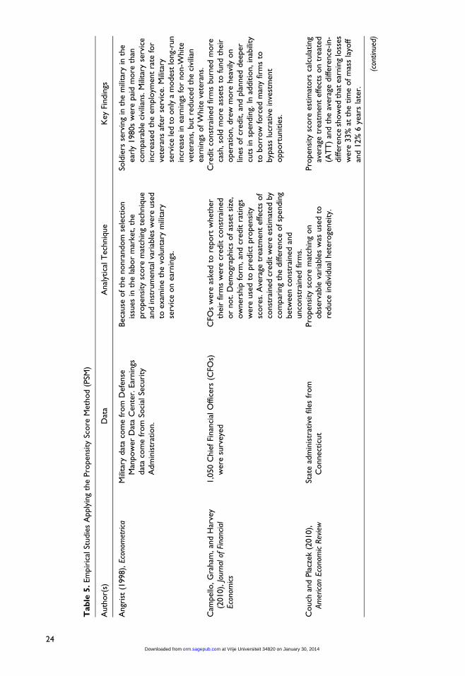
Tab

le5.

Em

pir

ical

Studie

sA

pply

ing

the

Pro

pen

sity

Score

Met

hod

(PSM

)

Auth

or(

s)D

ata

Anal

ytic

alT

echniq

ue

Key

Findin

gs

Angr

ist

(1998),

Eco

nom

etrica

Mili

tary

dat

aco

me

from

Def

ense

Man

pow

erD

ata

Cen

ter.

Ear

nin

gsdat

aco

me

from

Soci

alSe

curi

tyA

dm

inis

trat

ion.

Bec

ause

ofth

enonra

ndom

sele

ctio

nis

sues

inth

ela

bor

mar

ket,

the

pro

pen

sity

score

mat

chin

gte

chniq

ue

and

inst

rum

enta

lvar

iable

sw

ere

use

dto

exam

ine

the

volu

nta

rym

ilita

ryse

rvic

eon

earn

ings

.

Sold

iers

serv

ing

inth

em

ilita

ryin

the

earl

y1980s

wer

epai

dm

ore

than

com

par

able

civi

lians.

Mili

tary

serv

ice

incr

ease

dth

eem

plo

ymen

tra

tefo

rve

tera

ns

afte

rse

rvic

e.M

ilita

ryse

rvic

ele

dto

only

am

odes

tlo

ng-

run

incr

ease

inea

rnin

gsfo

rnon-W

hite

vete

rans,

but

reduce

dth

eci

vilia

nea

rnin

gsofW

hite

vete

rans.

Cam

pel

lo,G

raham

,an

dH

arve

y(2

010),

Jour

nalo

fFi

nanc

ial

Eco

nom

ics

1,0

50

Chie

fFi

nan

cial

Offic

ers

(CFO

s)w

ere

surv

eyed

CFO

sw

ere

aske

dto

report

whet

her

thei

rfir

ms

wer

ecr

edit

const

rain

edor

not.

Dem

ogr

aphic

sofas

set

size

,ow

ner

ship

form

,an

dcr

edit

ratings

wer

euse

dto

pre

dic

tpro

pen

sity

score

s.A

vera

getr

eatm

ent

effe

cts

of

const

rain

edcr

edit

wer

ees

tim

ated

by

com

par

ing

the

diff

eren

ceofsp

endin

gbet

wee

nco

nst

rain

edan

dunco

nst

rain

edfir

ms.

Cre

dit

const

rain

edfir

ms

burn

edm

ore

cash

,so

ldm

ore

asse

tsto

fund

thei

roper

atio

n,dre

wm

ore

hea

vily

on

lines

ofcr

edit,an

dpla

nned

dee

per

cuts

insp

endin

g.In

additio

n,in

abili

tyto

borr

ow

forc

edm

any

firm

sto

byp

ass

lucr

ativ

ein

vest

men

topport

unitie

s.

Couch

and

Pla

czek

(2010),

Am

eric

anEco

nom

icRev

iew

Stat

ead

min

istr

ativ

efil

esfr

om

Connec

ticu

tPro

pen

sity

score

mat

chin

gon

obse

rvab

leva

riab

les

was

use

dto

reduce

indiv

idual

het

eroge

nei

ty.

Pro

pen

sity

score

estim

ators

calc

ula

ting

aver

age

trea

tmen

tef

fect

son

trea

ted

(AT

T)

and

the

aver

age

diff

eren

ce-in-

diff

eren

cesh

ow

edth

atea

rnin

glo

sses

wer

e33%

atth

etim

eofm

ass

layo

ffan

d12%

6ye

ars

late

r.

(con

tinue

d)




Tab

le5.

(co

nti

nu

ed

)

Auth

or(

s)D

ata

Anal

ytic

alT

echniq

ue

Key

Findin

gs

Dru

cker

and

Puri

(2005),

Jour

nal

ofFi

nanc

eT

hey

com

bin

eddat

ase

tsfr

om

multip

ledat

abas

es.T

hey

colle

cted

dat

aon

seas

oned

equity

issu

ers,

incl

udin

gcr

edit

rating,

stock

retu

rn,le

ndin

ghis

tory

,an

din

sura

nce

his

tory

.

Pro

pen

sity

score

mat

chin

gw

asuse

dto

mat

chnon-c

urr

ent

loan

sto

curr

ents

loan

s.Pro

pen

sity

score

isca

lcula

ted

usi

ng

obse

rvat

ional

vari

able

sin

clud-

ing

cred

itra

ting,

firm

indust

ry,an

doth

erva

riab

les.

Ove

rall,

under

wri

ters

(com

mer

cial

ban

ksan

din

vest

men

tban

ks)

enga

ged

inco

ncu

rren

tle

ndin

gan

dpro

vide

dis

counts

.In

additio

n,co

ncu

rren

tle

ndin

ghel

ped

under

wri

ters

build

rela

tionsh

ips,

whic

hhel

punder

wri

ters

incr

ease

the

pro

bab

ility

ofre

ceiv

ing

curr

ent

and

futu

rebusi

nes

s.Fr

ank,

Akr

esh,an

dLu

(2010),

Am

eric

anSo

ciol

ogic

alRev

iew

Dat

aw

ere

colle

cted

from

New

Imm

igra

nt

Surv

eyw

ith

around

1,0

00

case

s.

They

use

dord

inal

logi

stic

model

toca

lcula

tepro

pen

sity

score

s,w

hic

hw

ere

use

dto

estim

ate

the

effe

ctof

skin

colo

ron

earn

ings

.

They

found

anav

erag

ediff

eren

ceof

$2,4

35.6

3diff

eren

cebet

wee

nlig

hte

ran

ddar

ker

skin

ned

indiv

idual

s.In

oth

erw

ord

s,dar

ker

skin

indiv

idual

sea

rnar

ound

$2,5

00

less

per

year

than

counte

rpar

ts.

Gan

gl(2

006),

Am

eric

anSo

ciol

ogic

alRev

iew

Surv

eyofIn

com

ean

dPro

gram

Par

tici

pat

ion

(SIP

P)

and

Euro

pea

nC

om

munity

House

hold

Pan

el(E

CH

P)

Diff

eren

ce-in-d

iffer

ence

pro

pen

sity

score

mat

chin

gG

angl

found

stro

ng

evid

ence

that

post

-unem

plo

ymen

tlo

sses

are

larg

ely

per

man

ent,

and

such

effe

ctis

par

ticu

larl

ysi

gnifi

cant

for

old

eran

dhig

h-w

age

work

ers

asw

ellas

for

fem

ale

emplo

yees

.G

rodsk

y(2

007),

Am

eric

anJo

urna

lof

Soci

olog

yD

ata

cam

efr

om

anum

ber

ofso

urc

es,

incl

udin

gth

ere

pre

senta

tive

sam

ple

sofst

uden

tsw

ho

com

ple

ted

hig

hsc

hoolin

1972,1982,an

d1992.

Inth

efir

stst

age,

pro

pen

sity

score

was

use

dto

adju

stfo

rse

lect

ion

on

obse

rvat

ional

vari

able

s.In

the

seco

nd

stag

e,th

eau

thor

exam

ined

the

type

ofco

llege

ast

uden

tw

illat

tend

contr

olli

ng

for

pro

pen

sity

score

s.

The

auth

or

found

the

evid

ence

that

aw

ide

range

ofin

stitutions

enga

gein

affir

mat

ive

action

for

Afr

ican

Am

eric

anst

uden

tsas

wel

las

for

His

pan

icst

uden

ts.

(con

tinue

d)




Tab

le5.

(co

nti

nu

ed

)

Auth

or(

s)D

ata

Anal

ytic

alT

echniq

ue

Key

Findin

gs

Hec

kman

,Ic

him

ura

,an

dT

odd

(1997),

Rev

iew

ofEco

nom

icSt

udie

s

The

Nat

ional

Job

Tra

inin

gPar

tner

ship

Act

(JT

PA

)an

dSu

rvey

ofIn

com

ean

dPro

gram

Par

tici

pat

ion

(SIP

P)

Pro

pen

sity

mat

chin

g,nonpar

amet

ric

conditio

nal

diff

eren

ce-in-d

iffer

ence

Aft

erdec

om

posi

ng

pro

gram

eval

uat

ion

bia

sin

toa

num

ber

ofco

mponen

ts,it

was

found

that

sele

ctio

nbia

sdue

tounobse

rvab

leva

riab

leis

less

import

ant

than

oth

erco

mponen

ts.

Mat

chin

gte

chniq

ue

can

pote

ntial

lyel

imin

ate

much

ofth

ebia

s.Le

chner

(2002),

Rev

iew

ofEco

nom

icSt

udie

sU

nem

plo

yed

indiv

idual

sin

Zuri

ch,a

regi

on

ofSw

itze

rlan

d,in

per

iods

1997-1

999.

Multin

om

ialm

odel

was

use

dto

estim

ate

pro

pen

sity

score

sofdis

cret

ech

oic

es(b

asic

trai

nin

g,fu

rther

trai

nin

g,em

plo

ymen

tpro

gram

,an

dte

mpora

ryw

age

subsi

dy)

.

The

empir

ical

evid

ence

reve

aled

support

for

the

fact

that

the

pro

pen

sity

score

mat

chin

gca

nbe

anin

form

ativ

eto

olto

adju

stfo

rin

div

idual

het

eroge

nei

tyw

hen

indiv

idual

shav

em

ultip

lepro

gram

sto

be

sele

cted

.M

alm

endie

ran

dT

ate

(2009),

Qua

rter

lyJo

urna

lof

Eco

nom

ics

Han

d-c

olle

cted

list

ofth

ew

inner

sof

CEO

awar

ds

bet

wee

n1975

and

2002

They

use

dpro

pen

sity

score

mat

chin

gto

crea

teco

unte

rfac

tual

sam

ple

for

non-

win

nin

gC

EO

s.N

eare

stnei

ghbor

mat

chin

gte

chniq

ue,

both

with

and

without

bia

sad

just

men

t,w

asuse

dto

iden

tify

the

counte

rfac

tual

sam

ple

.

They

found

that

awar

d-w

innin

gC

EO

sunder

per

form

ove

rth

e3

year

sfo

llow

ing

the

awar

d:R

elat

ive

under

per

form

ance

isbet

wee

n15%

to26%

.

Xuan

(2009),

Rev

iew

ofFi

nanc

ial

Stud

ies

S&P’s

exec

utive

com

pen

sation

bet

wee

n1993

and

2002

Ord

inar

yle

ast

squar

ew

asuse

das

the

maj

or

tech

niq

ue.

The

pro

pen

sity

score

met

hod

was

use

das

robust

chec

kto

addre

ssth

eis

sue

of

endoge

nous

sele

ctio

nofC

EO

.

Spec

ialis

tC

EO

s,def

ined

asC

EO

sw

ho

hav

epro

mote

dfr

om

ace

rtai

ndiv

isio

ns

ofth

eir

firm

,neg

ativ

ely

affe

ctse

gmen

tin

vest

men

tef

ficie

ncy

.




data to obtain equal distribution between the treated and control groups. Third, if treatment assign-

ment is strongly ignorable, scholars can use the PSM on observational data sets to estimate an ATT

that is reasonably close to the ATT calculated from experiments. Fourth, the matching technique, by

its nature, is nonparametric. Like other nonparametric approaches, this technique will not suffer

from problems that are prevalent in most parametric models, such as the assumption of distribution.

It generally outperforms simple regression analysis when the true functional form for the regression

is nonlinear (Morgan & Harding, 2006). Finally, the PSM is an intuitively sounder method for deal-

ing with covariates than is traditional regression analysis. For example, the idea that covariates in

both the treated group and the control group have the same distributions is much easier to understand

than the interpretation using ‘‘control all other variables at mean’’ or ‘‘ceteris paribus.’’ Even for

regression, without appropriately adjusting for the covariate distribution, one can get an ATT with

the regression technique despite the fact that no meaningful ATT exists.

Despite its many advantages, the PSM also has its limitations. Like other nonparametric tech-

niques, the PSM generally has no test statistics. Although the bootstrap technique can be used to

estimate the variance, such techniques are not fully justified or widely accepted by researchers

(Imbens, 2004). Hence, the use of the PSM may be limited because while it can help scholars draw

causal inferences, it cannot help with drawing statistical inferences. Another key hurdle of this

method is that there are currently no established procedures to investigate whether treatment assign-

ment is strongly ignorable. Heckman et al. (1998) demonstrated that the PSM cannot eliminate bias

due to unobservable differences across groups. The PSM can reweight observational covariates, but

it cannot deal with unobservable variables. Some unobservable variables (e.g., environmental con-

text, region) can increase the bias of the ATT estimated using the PSM. Third, even when the treat-

ment assignment is strongly ignorable, the accuracy of the ATT estimated by the PSM depends on

the quality of the observational data. Thus, measurement error (cf. Gerhart, Wright, & McMahan,

2000) and nonrandom missing values can affect the estimated ATT. Finally, although there are a

few propensity score matching techniques, one can find little guidance on which types of matching

techniques work best for different applications.

Overall, despite its shortcomings, the PSM can be employed by management scholars to inves-

tigate the ATT of management interventions. Appropriately used, the PSM can eliminate bias due to

nonoverlapping distributions between the treatment and the control groups. The PSM can also

reduce the problem of unfair comparison. However, scholars must be careful about the quality of

the data because the effectiveness of the PSM depends on the observational covariates. Research

using objective measures will be an optimal setting for using the PSM. In empirical settings with

low quality data, scholars can implement nonparametric PSM as a robust test to justify the para-

metric findings generated by traditional econometric models.

To draw meaningful and honest causal inferences, one must appropriately choose the technique

that works best for testing the causal relationship. When one has collected panel data and believes

that omitted variable is time-invariant, then the fixed effects model is the best choice for estimating

bias due to an omitted variable (Allison, 2009; Beck et al., 2008). When one finds one or more per-

fect instrumental variables, using two-stage least-squares (2SLS) can also address the bias of causal

effects calculated through conventional regression techniques. When the endogenous variable suf-

fers only from measurement error and when one knows the reliability coefficient, one can use regres-

sion analysis and correct the bias using the reliability coefficient. Almost no technique is perfect in

drawing an unbiased causal inference, including experimental design. Heckman and Vytlacil (2007)

remarked that explicitly manipulating treatment assignment cannot always represent the real-world

problem because experimentation naturally discards information contained in a real-world context

that includes dropout, self-selection, and noncompliance.

Sometimes a combination of techniques is also recommended. For example, to alleviate the extra-

polation bias in the regression models Imbens and Wooldridge (2009) recommend using matching to

Li 27




generate a balanced sample. Similarly, Rosenbaum and Rubin (1983) suggested that differences

due to unobserved heterogeneity should be addressed after balancing the observed covariates.

Additionally, the PSM can also be incorporated in studies using the longitudinal design. Readers

who are interested in estimating the ATT using longitudinal data can also refer to the nonpara-

metric conditional difference-in-difference model (Heckman et al., 1997) and the semiparametric

conditional difference-in-difference model (Heckman et al., 1998). To conclude, to draw the best

causal inference, one needs to choose the appropriate methods. Of various techniques, the PSM

should be a potential choice.

Conclusion

The purpose of this article is to introduce the PSM to the management field. This article makes

several contributions to organizational research methods literature. First, it not only advances

management scholars’ understanding of a neglected method to estimate causal effects, but also

discusses some of the technique’s limitations. Second, by integrating previous work on the PSM,

it provides a step-by-step flowchart that management scholars can easily implement in their

empirical studies. The attached data set with SPSS and STATA stratified matching codes help

management scholars to calculate the ATT. Readers can make context-dependent decisions and

choose a matching algorithm that is most beneficial for their objectives. Finally, a brief review

of the applications of the PSM in other social science fields and a discussion of potential usage

of the PSM in the management field provides an overview of how management scholars can

employ the PSM in future empirical studies.

Appendix A

Boosted Regression

Boosted regression (or boosting) is a general, automated, data-mining technique that has shown

considerable success in using a large number of covariates to predict treatment assignment and fit

a nonlinear surface (McCaffrey, Ridgeway, & Morral, 2004). Boosting relies on a regression tree

using a recursive algorithm to estimate the function that describes the relationship between a set of

covariates and the dependent variable. The regression tree begins with a complete data set and then

partitions the data set into two regions by a series of if-then statements (Schonlau, 2005). For

example, if age and race are covariates, the algorithm can first split the data set into two regions

based on the condition of either of these two variables. The splitting algorithm continues recur-

sively until the regression tree reaches the allowable number of splits. Friedman (2001) has shown

that boosted regression outperforms other methods in reducing prediction error. McCaffrey et al.

(2004) summarized three important advantages of the boosting technique. First, regression trees

are easy and fast to fit. Second, regression trees can handle different types of covariates including

continuous, nominal, ordinal, and missing variables. When boosted logistic regression is used to

predict propensity scores, the use of different forms of covariates generally produces exactly the

same propensity score adjustment. Finally, the boosting technique is capable of handling many

covariates, even those unrelated to treatment assignment or correlated with one another. Schonlau

(2005) listed factors that favor the use of the boosting technique. These factors include a large data

set, suspected nonlinearities, more variables than observations, suspected interactions, correlated

data, and ordered categorical covariates. He concludes that the boosting technique does not require

scholars to specify interactions and nonlinearities. Thus, the boosting technique can simplify the

procedure of computing propensity scores by reducing the burden of adding high-order covariates

such as interactions.





Ap

pen

dix

B.

ASm

allD

ata

Set

for

Man

ual

lyC

alcu

lating

Ave

rage

Tre

atm

ent

Effec

ton

the

Tre

ated

Gro

up

(AT

T)

Cas

eID

Step

1St

ep2

Step

3:Est

imat

eC

ausa

lEffec

t

Outc

om

eT

reat

men

tA

gePSc

ore

Blo

ckID

Tpsc

ore

Tag

eY i

TY j

CN

qT

NqC

AT

Tq¼

15

Wei

ght

AT

T�

Wei

ght

11,0

048.5

40

50

0.0

76

11.3

20.1

67

49,2

37.6

60

31,4

01.6

87

25

18,3

38.4

926

0.0

81,4

67.0

79

20

019

0.1

09

13

2,0

688.1

70

26

0.1

28

14

00

44

0.1

41

5664.9

77

039

0.1

77

16

36,6

46.9

51

35

0.0

75

17

12,5

90.7

11

33

0.1

01

18

24,6

42.5

70

32

0.2

65

21.0

00.1

36

42,4

65.3

15

44,7

75.1

21

45

1,6

61.3

0455

0.1

6265.8

09

910,3

44.0

90

44

0.2

68

210

9,7

88.4

61

041

0.2

82

211

00

33

0.3

13

212

00

20

0.3

65

213

13,1

67.5

21

22

0.2

61

214

4,3

21.7

05

126

0.3

12

215

12,5

58.0

21

46

0.3

61

216

12,4

18.0

71

46

0.3

92

217

00

40

0.4

12

31.8

60.0

25

33,3

13.7

04

39,8

98.6

20

45

348.7

02

0.1

655.7

92

18

17,7

32.7

20

26

0.4

56

319

4,4

33.1

80

30

0.4

81

320

00

21

0.5

13

321

17,7

32.7

20

20

0.5

58

322

7,2

84.9

86

141

0.5

11

323

5,5

22.7

88

117

0.5

25

324

20,5

05.9

31

24

0.5

47

325

01

27

0.5

93

26

2,3

64.3

63

041

0.6

78

40.8

01.5

61

21,6

07.0

32

31,9

78.0

05

63

–7,0

58.1

63

0.2

4–1,6

93.9

59

27

22,1

65.9

023

0.7

27

428

7,4

47.7

42

024

0.7

46

429

2,1

64.0

22

121

0.6

54

430

11,1

41.3

91

23

0.7

39

431

3,4

62.5

64

129

0.7

58

432

559.4

43

120

0.7

59

433

4,2

79.6

13

119

0.7

64

434

01

23

0.7

68

4

(con

tinue

d)




Ap

pen

dix

B.

(co

nti

nu

ed

)

Cas

eID

Step

1St

ep2

Step

3:Est

imat

eC

ausa

lEffec

t

Outc

om

eT

reat

men

tA

gePSc

ore

Blo

ckID

Tpsc

ore

Tag

eY i

TY j

CN

qT

NqC

AT

Tq¼

15

Wei

ght

AT

T�

Wei

ght

35

5,6

15.3

61

028

0.9

23

51.2

30.5

52

65,4

59.1

09

5,6

15.3

61

92

4,4

65.5

53833

0.3

61,6

07.5

99

36

00

23

0.9

54

537

13,3

85.8

61

18

0.9

13

538

8,4

72.1

58

127

0.9

48

539

01

18

0.9

54

540

6,1

81.8

81

17

0.9

59

541

289.7

91

21

0.9

61

542

17,8

14.9

81

37

0.9

65

543

9,2

65.7

88

117

0.9

66

544

1,9

23.9

38

125

0.9

75

45

8,1

24.7

15

125

0.9

87

546

11,8

21.8

10

53

0.0

01

Unm

atch

edca

ses

AT

T¼

1,7

02.3

21

47

24,8

25.8

10

52

0.0

03

48

33,9

87.7

10

28

0.0

09

49

33,9

87.7

10

41

0.0

13

50

54,6

75.8

80

38

0.0

16

Note

:PSc

ore¼

pro

pen

sity

score

s;T

age/T

psc

ore¼

t-te

stfo

rag

ean

dpro

pen

sity

score

sin

each

bal

ance

dblo

ck;Y

iT¼

sum

mat

ion

ofo

utc

om

eva

riab

lefo

rtr

eate

dca

ses

inea

chblo

ck;Y

iC¼

sum

ma-

tion

ofoutc

om

eva

riab

lefo

rco

ntr

olca

ses

inea

chblo

ck;N

qT¼

tota

lnum

ber

oftr

eate

dca

ses

inea

chblo

ck;N

qC¼

tota

lnum

ber

ofco

ntr

olca

ses

inea

chblo

ck;A

TT

q¼

15¼

YiT

/NqT

–Y

iC/N

qC;

aver

age

trea

tmen

tef

fect

for

each

bal

ance

dblo

ck;w

eigh

t¼

tota

lnum

ber

oftr

eate

dca

ses

inea

chblo

ckdiv

ided

by

tota

lnum

ber

oftr

eate

dca

ses

inth

esa

mple

.




Appendix C

SPSS Code for Stratified Matching

*Step 1: Calculate propensity score.LOGISTIC REGRESSION VARIABLES TREATMENT

/METHOD¼ENTER X1 X2 X3/SAVE¼PRED/CRITERIA¼PIN(.05) POUT(.10) ITERATE(20) CUT(.5).

RENAME VARIABLES (PRE_1¼pscore).

The above code calculates predicted probability using a number of observation variables (e.g. X1,

X2, and X3). Readers can change their variables correspondingly.

*Step 2: Stratify into five blocks.compute blockid¼.if (pscore<¼ .2) & (pscore > .05) blockid¼1.if (pscore<¼ .4) & (pscore > .2) blockid¼2.if (pscore<¼ .6) & (pscore > .4) blockid¼3.if (pscore<¼ .8) & (pscore > .6) blockid¼4.if ( pscore > .8) blockid¼5.execute.*Perform t test for each block.*Split file first, and then excute t test.SORT CASES BY blockid.SPLIT FILE SEPARATE BY blockid.T-TEST GROUPS¼treatment(0 1)

/MISSING¼ANALYSIS/VARIABLES¼age pscore/CRITERIA¼CI(.95).

The above code first stratifies variables into five blocks, and then carries on the t-test for each of

the blocks. SPSS has no ‘‘if’’ option for t-test, thus it is important to split the data based on block ID,

and then conduct the t-test.

*Step 3: Perform Stratification Matching Procedure.*Caclulate YiT and YjC in Appendix B.AGGREGATE

/OUTFILE¼* MODE¼ADDVARIABLES/BREAK¼blockid treatment/outcome_sum¼SUM(outcome).

*Calculate NqT and NqC in Appendix B.AGGREGATE

/OUTFILE¼* MODE¼ADDVARIABLES/BREAK¼blockid treatment/N_BREAK¼N.

*Calculate total number of treatment cases.AGGREGATE

/OUTFILE¼* MODE¼ADDVARIABLES/BREAK¼/N_Treatment¼sum(treatment).

Li 31




COMPUTE ATTQ¼outcome_sum/N_BREAK.EXECUTE.DATASET DECLARE agg_all.AGGREGATE

/OUTFILE¼’agg_all’/BREAK¼treatment blockid/N_Block_T¼MEAN(N_BREAK)/ATTQ_T¼MEAN(ATTQ)/N_Treatment¼MEAN(N_Treatment).

DATASET ACTIVATE agg_all.DATASET COPY agg_treat.DATASET ACTIVATE agg_treat.FILTER OFF.USE ALL.SELECT IF (treatment ¼ 1).EXECUTE.DATASET ACTIVATE agg_all.

DATASET COPY agg_control.DATASET ACTIVATE agg_control.FILTER OFF.USE ALL.SELECT IF (treatment¼0&blockid<6).EXECUTE.DATASET ACTIVATE agg_control.

RENAME VARIABLES (N_Block_T ATTQ_T ¼N_Block_C ATTQ_C ).

MATCH FILES /FILE¼*/FILE¼’agg_treat’/RENAME (blockid N_Treatment treatment ¼ d0 d1 d2)/DROP¼ d0 d1 d2.

EXECUTE.

COMPUTE ATTQ¼ATTQ_T-ATTQ_C.EXECUTE.COMPUTE weight¼N_Block_T/N_Treatment.EXECUTE.COMPUTE ATTxweight¼ATTQ*weight.EXECUTE.AGGREGATE

/OUTFILE¼* MODE¼ADDVARIABLES OVERWRITEVARS¼YES/BREAK¼/ATTxweight_sum¼SUM(ATTxweight).

DATASET CLOSE agg_all.DATASET CLOSE agg_control.DATASET CLOSE agg_treat.





This step computes each of the components in Equation 2.2. For example, it first calculates the

number of treated cases and the number of control cases in each matched block. Then, it also gauges

the summation of outcome in each balanced blocks. The code then extracts each of the necessary

components into two different data sets: agg_control and agg_treat. Finally, the code matches these

two data sets based on block ID and estimates the ATT. The final result will be displayed in the vari-

able called ‘‘ATTxweight.’’

Appendix D

STATA Code for Stratified Matching

*STEP 1: get the propensity scores using logistical regression*Choose covariates appropriatelylogit treatment X1 X2 X3*Calculate propensity scorespredict pscore, p

*STEP 2: subclassificationgen blockid¼.replace blockid¼1 if pscore<¼.2 & pscore>.05replace blockid¼2 if pscore<¼.4 & pscore> .2replace blockid¼3 if pscore<¼.6 & pscore> .4replace blockid¼4 if pscore<¼.8 & pscore> .6replace blockid¼5 if pscore>.8

*STEP 2: t test for balance in each blockforeach var of varlist age pscore f

forvalues i¼1/5 fttest ‘var’ if blockid ¼¼‘i’, by(treatment)g

g

*STEP 3: Estimate causal effects using stratified matchingsort blockid treatmentgen YTQ¼. *Yic in Appendix B tablegen TTN¼1 *Nqt in Appendix B tablegen YCQ¼. *Yjc in Appendix B tablegen TCN¼1 *Nqc in Appendix B tableforvalues i¼1/5 f

*Get sum for outcome in each treated blocksum outcome if treatment¼¼1 & blockid¼¼‘i’replace YTQ¼r(sum) if blockid¼¼‘i’*Number of treated cases in each blocksum TTN if treatment¼¼1 & blockid¼¼‘i’replace TTN¼r(sum) if blockid¼¼‘i’*Get sum for outcome in each control blocksum outcome if treatment¼¼0 & blockid¼¼‘i’replace YCQ¼r(sum) if blockid¼¼‘i’*Number of treated cases in each blocksum TCN if treatment¼¼0 & blockid¼¼‘i’

Li 33




replace TCN¼r(sum) if blockid¼¼‘i’g

gen ATTQ¼YTQ/TTN-YCQ/TCN*Weights for ATTsum treatmentgen W¼TTN/r(sum)*Weighted ATTgen ATT¼ATTQ*Wbysort blockid: gen id¼_nsum ATT if id¼¼1display "The ATT is ‘r(sum)’"

Appendix E.

Software Packages for Applying the Propensity Score Method (PSM)

Environment Software Name Authors Function and Download Sources

R Matching Sekhon (2007) Relies on an automated procedure to detectmatches based on a number of univariateand multivariate metrics. It performspropensity matching, primarily 1:Mmatching. The package also allows matchingwith and without replacement.Download source:http://sekhon.berkeley.edu/matching/Document:http://cran.r-project.org/web/packages/Matching/Matching.pdf

PSAgraphics Helmreich and Pruzek(2009)

Provides enriched graphical tools to testwithin strata balance. It also providesgraphical tools to detect covariatedistributions across strata.Download source:http://cran.r-project.org/web/packages/PSAgraphics/index.html

Twang Ridgeway, McCaffrey,and Morral (2006)

Includes propensity score estimating andweighting. Generalized boosted regressionis used to estimate propensity scores thussimplifying the procedure to estimatepropensity scores.Download source:http://cran.r-project.org/web/packages/twang/index.html

SAS Greedy matching Kosanke and Bergstralh(2004)

Performs 1:1 nearest neighbor matching.Download source: http://mayoresearch.mayo.edu/mayo/research/biostat/upload/gmatch.sas

OneToManyMTCH Parsons (2004) Allows users to specify the propensity scorematching from 1:1 or 1:M.Download source:http://www2.sas.com/proceedings/sugi29/165-29.pdf

(continued)





Acknowledgments

Special thanks to Barry Gerhart for his invaluable support and to Associate Editor James LeBreton and anon-

ymous reviewers for their constructive feedbacks. This article has also benefited from suggestions by Russ

Coff, Jose Cortina, Cindy Devers, Jon Eckhardt, Phil Kim, and seminar participants at 2011 AOM conference.

Declaration of Conflicting Interests

The author(s) declared no potential conflicts of interest with respect to the research, authorship, and/or publi-

cation of this article.

Funding

The author(s) received no financial support for the research, authorship, and/or publication of this article.

Notes

1. Harder, Stuart, and Anthony (2010) argued that propensity score method (PSM) can be used to estimate the

average treatment effect on the treated group (ATT), and subclassifying the propensity score can be used to

calculate the average treatment effect (ATE). However, economists typically viewed the PSM as a technique

to estimate the ATT (Dehejia & Wahba, 1999, 2002). Following Dehejia and Wahba (1999, 2002), the

remaining section regards the PSM as a way to calculate the ATT. The remaining sections use causal effects,

treatment effects, and ATT interchangeably.

2. Psychology scholars also extended this to develop the causal steps approach to draw mediating causal infer-

ence (e.g., Baron & Kenny, 1986). It is beyond the scope of this article to fully discuss mediation. Interested

readers can read LeBreton, Wu, and Bing (2008) and Wood, Goodman, Beckmann, and Cook (2008) for

surveys.

3. Becker and Ichino (2002) have written a nice STATA program (pscore) to estimate the propensity score. The

convenience of using pscore is that the program can stratify propensity scores to a specified number of

blocks and test the balance of propensity scores in each block. However, when there is more than one treat-

ment, it is inappropriate to use pscore to estimate the propensity score.

Appendix E. (continued)

Environment Software Name Authors Function and Download Sources

SPSS SPSS Macro for Pscore matching

Painter (2004) Performs nearest neighbor propensity scorematching. It seems to solely do 1:1 matchingwithout replacement.Download source:http://www.unc.edu/*painter/SPSSsyntax/propen.txt

STATA Pscore Becker and Ichino (2002) Estimates propensity scores and conducts anumber of matching such as radius, nearestneighbor, kernel, and stratified.Download source:http://www.lrz.de/*sobecker/pscore.html

Psmatch2 Leuven and Sianesi(2003)

Allows a number of matching procedures,including kernel matching and k:1 matching.It also supports common support graphsand balance testing.Download source:http://ideas.repec.org/c/boc/bocode/s432001.html

Li 35




4. Propensity score matching is one technique of many matched sampling technique. One can use exact match-

ing simply based on one or more covariates. For example, scholars may match sample based on standard

industry classification (SIC) and firm size rather than matching using propensity scores.

5. These components are: the variance of the covariates in the control groups, the variance of the covariates in

the treated groups, the mean of the covariates in the control groups, the mean of the covariates in the treated

groups, and the estimated propensity score. The variance of the covariates in the treated and the control

groups are weighted by the propensity score.

6. Instrumental variable (IV) is typically used by scholars under the condition of simultaneity. Because of the

difficulty in finding an IV, it is not viewed as a general remedy for endogeneity issues.

References

Allison, P. (2009). Fixed effects regression models. Newbury Park, CA: Sage.

Angrist, J. (1998). Estimating the labor market impact of voluntary military service using social security data on

military applicants. Econometrica, 66, 249-288.

Angrist, J. D., Imbens, G. W., & Rubin, D. B. (1996). Identification of causal effects using instrumental vari-

ables. Journal of the American Statistical Association, 9, 444-455.

Antonakis, J., Bendahan, S., Jacquart, P., & Lalive, R. (2010). On making causal claims: A review and recom-

mendations. The Leadership Quarterly, 21(6), 1086-1120.

Arceneaux, K., Gerber, A., & Green, D. (2006). Comparing experimental and matching methods using a large-

scale voter mobilization experiment. Political Analysis, 14, 1-26.

Baron, R. M., & Kenny, D. A. (1986). The moderator-mediator variable distinction in social psychological

research: Conceptual, strategic, and statistical considerations. Journal of Personality and Social

Psychology, 51(6), 1173-1182.

Beck, N., Bruderl, J., & Woywode, M. (2008). Momentum or deceleration? Theoretical and methodolo-

gical reflections on the analysis of organizational change. Academyof Management Journal, 51(3),

413-435.

Becker, S., & Caliendo, M. (2007). Sensitivity analysis for average treatment effects. Stata Journal, 7(1), 71-83.

Becker, S., & Ichino, A. (2002). Estimation of average treatment effects based on propensity scores. The Stata

Journal, 2, 358-377.

Berk, R. A. (1983). An introduction to sample selection bias in sociological data. American Sociological

Review, 48(3), 386-398.

Campello, M., Graham, J., & Harvey, C. (2010). The real effects of financial constraints: Evidence from a

financial crisis. Journal of Financial Economics, 97, 470-487.

Cochran, W. (1957). Analysis of covariance: Its nature and uses. Biometrics, 13(3), 261-281.

Cochran, W. (1968). The effectiveness of adjustment by subclassification in removing bias in observational

studies. Biometrics, 24, 295-313.

Couch, K. A., & Placzek, D. W. (2010). Earnings losses of displaced workers revisited. American Economic

Review, 100, 572-589.

Cox, D. (1992). Causality: Some statistical aspects. Journal of the Royal Statistical Society, Series A (Statistics

in Society), 155, 291-301.

Dehejia, R., & Wahba, S. (1999). Causal effects in nonexperimental studies: Reevaluating the evaluation of

training programs. Journal of the American Statistical Association, 94, 1053-1062.

Dehejia, R., & Wahba, S. (2002). Propensity score-matching methods for nonexperimental causal studies.

Review of Economics and Statistics, 84, 151-161.

DiPrete, T. A., & Gangl, M. (2004). Assessing bias in the estimation of causal effects: Rosenbaum bounds on

matching estimators and instrumental variables estimation with imperfect instruments. Sociological

Methodology, 34, 271-310.

Duncan, O. D. (1975). Introduction to structural equation models. San Diego, CA: Academic Press.





Drucker, S., & Puri, M. (2005). On the benefits of concurrent lending and underwriting. Journal of Finance,

60(6), 2763-2799.

Efron, B., & Tibshirani, R. (1997). An introduction to the bootstrap. London: Chapman & Hall.

Frank, R., Akresh, I. R., & Lu, B. (2010). Latino Immigrants and the US racial order: How and where do they fit

in? American Sociological Review, 75(3), 378-401.

Friedman, J. H. (2001). Greedy function approximation: A gradient boosting machine. The Annals of Statistics,

29, 1189-1232.

Gangl, M. (2006). Scar effects of unemployment: An assessment of institutional complementarities. American

Sociological Review, 71(6), 986-1013.

Gerhart, B. (2007). Modeling human resource management and performance linkages. In P. Boxall, J. Purcell,

& P. Wright (Eds.), The Oxford handbook of human resource management (pp. 552-580). Oxford: Oxford

University Press.

Gerhart, B., Wright, P., & McMahan, G. (2000). Measurement error in research on the human resources and

firm performance relationship: Further evidence and analysis. Personnel Psychology, 53, 855-872.

Greene, W. (2008). Econometric analysis (6th ed.). Upper Saddle River, NJ: Prentice Hall.

Grodsky, E. (2007). Compensatory sponsorship in higher education. American Journal of Sociology, 112(6),

1662-1712.

Gu, X., & Rosenbaum, P. (1993). Comparison of multivariate matching methods: Structures, distances, and

algorithms. Journal of Computational and Graphical Statistics, 2, 405-420.

Harder, V. S., Stuart, E. A., & Anthony, J. C. (2010). Propensity score techniques and the assessment of mea-

sured covariate balance to test causal associations in psychological research. Psychological Methods, 15,

234-249.

Hamilton, B. H., & Nickerson, J. A. (2003). Correcting for endogeneity in strategic management research.

Strategic Organization, 1, 51-78.

Heckman, J. (1979). Sample selection bias as a specification error. Econometrica, 47, 153-161.

Heckman, J., & Hotz, V. (1989). Choosing among alternative nonexperimental methods for estimating the

impact of social programs: The case of manpower training. Journal of the American Statistical

Association, 84, 862-874.

Heckman, J., Ichimura, H., Smith, J., & Todd, P. (1998). Characterizing selection bias using experimental data.

Econometrica, 66, 1017-1098.

Heckman, J., Ichimura, H., & Todd, P. E. (1997). Matching as an econometric evaluation estimator: Evidence

from evaluating job training program. Review of Economic Studies, 64, 605-654.

Heckman, J. J., & Vytlacil, E. J. (2007). Econometric evaluation of social programs, part II: Using the marginal

treatment effect to organize alternative econometric estimators to evaluate social programs, and to forecast

their effects in new environments. Handbook of Econometrics, 6, 4875-5143.

Helmreich, J. E., & Pruzek, R. M. (2009). PSAgraphics: An R package to support propensity score analysis.

Journal of Statistical Software, 29, 1-23.

Hoetker, G. (2007). The use of logit and probit models in strategic management research: Critical issues.

Strategic Management Journal, 28(4), 331-343.

Imbens, G. (2000). The role of the propensity score in estimating dose-response functions. Biometrika, 87(3),

706-710.

Imbens, G. W. (2004). Nonparametric estimation of average treatment effects under exogeneity: A review. The

Review of Economics and Statistics, 86, 4-29.

Imbens, G. W., & Wooldridge, J. M. (2009). Recent developments in the econometrics of program evaluation.

Journal of Economic Literature, 47(1), 5-86.

James, L. R. (1980). The unmeasured variables problem in path analysis. Journal of Applied Psychology, 65(4),

415-421.

James, L. R., Mulaik, S. A., & Brett, J. M. (1982). Causal analysis: Assumptions, models, and data. Thousand

Oaks, CA: Sage.

Li 37




Joffe, M. M., & Rosenbaum, P. R. (1999). Invited commentary: Propensity scores. American Journal of

Epidemiology, 150, 327-333.

King, G., Keohane, R. O., & Verba, S. (1994). Designing social inquiry: Scientific inference in qualitative

research. Princeton, NJ: Princeton University Press.

Kosanke, J., & Bergstralh, E. (2004). gmatch: Match 1 or more controls to cases using the GREEDY algorithm.

Retrieved from http://mayoresearch.mayo.edu/mayo/research/biostat/upload/gmatch.sas (accessed May 15,

2012)

Lalonde, R. J. (1986). Evaluating the econometric evaluations of training programs with experimental data.

American Economic Review, 76, 604-620.

LeBreton, J. M., Wu, J., & Bing, M. N. (2008). The truth(s) on testing for mediation in the social and organiza-

tional sciences. In C. E. Lance, & R. J. Vandenberg (Eds.), Statistical and methodological myths and urban

legends (pp. 107-140). New York, NY: Routledge.

Lechner, M. (2002). Program heterogeneity and propensity score matching: An application to the evaluation of

active labor market policies. Review of Economics and Statistics, 84, 205-220.

Leuven, E., & Sianesi, B. (2003). PSMATCH2: Stata module to perform full Mahalanobis and propensity score

matching, common support graphing, and covariate imbalance testing [Statistical software components].

Boston, MA: Boston College.

Li, Y., Propert, K., & Rosenbaum, P. (2001). Balanced risk set matching. Journal of the American Statistical

Association, 96, 870-882.

Long, J. S. (1997). Regression models for categorical and limited dependent variables. Thousand Oaks, CA:

Sage.

Malmendier, U., & Tate, G. (2009). Superstar CEOs. The Quarterly Journal of Economics, 124(4),

1593-1638.

McCaffrey, D. F., Ridgeway, G., & Morral, A. R. (2004). Propensity score estimation with boosted regression

for evaluating causal effects in observational studies. Psychological Methods, 9, 403-425.

Mellor, S., & Mark, M. M. (1998). A quasi-experimental design for studies on the impact of administrative

decisions: Applications and extensions of the regression-discontinuity design. Organizational Research

Methods, 1(3), 315-333.

Morgan, S. L., & Harding, D. J. (2006). Matching estimators of causal effects—Prospects and pitfalls in theory

and practice. Sociological Methods & Research, 35, 3-60.

Morgan, S. L., & Winship, C. (2007). Counterfactuals and causal inference: Methods and principles for social

research. Cambridge, UK: Cambridge University Press.

Painter, J. (2004). SPSS Syntax for nearest neighbor propensity score matching. Retrieved from http://www.

unc.edu/~painter/SPSSsyntax/propen.txt (accessed May 15, 2012)

Parsons, L. (2004). Performing a 1: N case-control match on propensity score. Proceedings of the 29th Annual

SAS Users Group International Conference, SAS Institute, Montreal, Canada.

Ridgeway, G., McCaffrey, D., & Morral, A. (2006). Toolkit for weighting and analysis of nonequivalent

groups: A tutorial for the twang package. Santa Monica, CA: RAND Corporation.

Rosenbaum, P. (1987). The role of a second control group in an observational study. Statistical Science, 2,

292-306.

Rosenbaum, P. (2002). Observational studies. New York, NY: Springer-Verlag.

Rosenbaum, P. (2004). Matching in observational studies. In A. Gelman & X. Meng (Eds.), Applied Bayesian

modeling and causal inference from an incomplete-data perspective (pp. 15-24). New York, NY: Wiley.

Rosenbaum, P. R., & Rubin, D. B. (1983). The central role of propensity score in observational studies for

causal effects. Biometrika, 70, 41-55.

Rosenbaum, P., & Rubin, D. (1984). Reducing bias in observational studies using subclassification on the

propensity score. Journal of the American Statistical Association, 79, 516-524.

Rosenbaum, P., & Rubin, D. (1985). Constructing a control group using multivariate matched sampling

methods that incorporate the propensity score. American Statistician, 39, 33-38.





Rousseau, D. (2006). Is there such a thing as evidence-based management. Academy of Management Review,

31, 256-269.

Rubin, D. (1997). Estimating causal effects from large data sets using propensity scores. Annals of Internal

Medicine, 127, 757-763.

Rubin, D. (2001). Using propensity scores to help design observational studies: Application to the tobacco liti-

gation. Health Services and Outcomes Research Methodology, 2(3), 169-188.

Rubin, D. (2004). Teaching statistical inference for causal effects in experiments and observational studies.

Journal of Educational and Behavioral Statistics, 29, 343-367.

Rynes, S., Giluk, T., & Brown, K. (2007). The very separate worlds of academic and practitioner periodicals in

human resource management: Implications for evidence-based management. Academy of Management

Journal, 50(5), 987-1008.

Schonlau, M. (2005). Boosted regression (boosting): An introductory tutorial and a Stata plugin. Stata Journal,

5, 330-354.

Sekhon, J. S. (2007). Multivariate and propensity score matching software with automated balance optimiza-

tion: The matching package for R. Journal of Statistical Software, 10(2), 1-51.

Simith, J., & Todd, P. E. (2005). Does matching overcome Lalonde’s critique of nonexperimental estimators.

Journal of Econometrics, 125, 305-353.

Steiner, P. M., Cook, T. D., Shadish, W. R., & Clark, M. H. (2010). The importance of covariate selection in

controlling for selection bias in observational studies. Psychological Methods, 15, 250-267.

Wasserman, N. (2003). Founder-CEO succession and the paradox of entrepreneurial success. Organization

Science, 14(2), 149-172.

Wolfe, F., & Michaud, K. (2004). Heart failure in rheumatoid arthritis: Rates, predictors, and the effect of

anti-tumor necrosis factor therapy. American Journal of Medicine, 116, 305-311.

Wood, R. E., Goodman, J. S., Beckmann, N., & Cook, A. (2008). Mediation testing in management research:

A review and proposals. Organizational Research Methods, 11(2), 270-295.

Wooldridge, J. (2002). Econometric analysis of cross section and panel data. Cambridge, MA: MIT Press.

Xuan, Y. (2009). Empire-building or bridge-building? Evidence from new CEOs’ internal capital allocation

decisions. Review of Financial Studies, 22, 4919-4918.

Bio

Mingxiang Li is a doctoral candidate at the Wisconsin School of Business, University of Wisconsin-Madison.

In addition to research methods, his current research interests include corporate governance, social network,

and entrepreneurship.

Li 39




using the propensity score the author(s) 2012 method to ... · introduces the propensity score...

Documents