Using Weibull accelerated failure time regression model topredict survival time and life expectancy

Enwu Liu1,2*

1 Musculoskeletal Health and Ageing Research Program, Mary MacKillop Institute forHealth Research, Australian Catholic University, Melbourne, Victoria, Australia2 College of Medicine and Public Health, Flinders University, Adelaide, South Australia,Australia

* enwu.liu@acu.edu.au

Abstract

Predict mean time to failure (MTTF) or mean time between failures(MTBF) andmedian survival time are quite common in Engineering reliability researches. In medicalliterature most prediction models are used to predict probabilities during a certainperiod. In this paper we introduced detailed calculations to predict different survivaltimes using Weibull accelerated failure time regression model and assessed the accuracyof the point predictions. The method to construct confidence interval for the predictedsurvival time was also discussed.

Weibull distribution 1

The Weibull distribution is also called type III extreme value distribution. [1] The 2

distribution has three parameters, the location parameter µ, the scale parameter ρ and 3

the shape parameter γ. The location parameter µ was predetermined as the minimum 4

value in the distribution, we usually choose 0 as the minimum value for survival 5

analysis, therefore, the distribution is reduced to a two-parameter distribution. 6

The cumulative distribution function(CDF) for a two parameter Weibull distributed 7

random variable T ∼W (ρ, γ) is given as 8

FT (t; ρ, γ) = 1− exp

[−(

t

ρ)γ]

(1)

for t ≥ 0, ρ > 0, γ > 0 and F (t; ρ, γ) = 0 for t < 0 9

The probability density function(PDF) of the Weibull distribution is given as 10

fT (t; ρ, γ) = F′(t; ρ, γ) =

γ

ρ(t

ρ)γ−1 exp

[−(

t

ρ)γ]

(2)

The survival function of the Weibull distribution is given as 11

ST (t) = 1− FT (t) = exp

[−(

t

ρ)γ]

(3)

June 23, 2018 1/14

The mean survival time or mean time to failure(MTTF) is given as

E(T ) =

∫ ∞0

S(t)dt (Darth Vader rule)

=

∫ ∞0

exp

[−(

t

ρ)γ]dt let (

t

ρ)γ = u⇒ t = ρu

1γ

=

∫ ∞0

e−uρ1

γu

1γ−1du

= ρ1

γΓ(

1

γ) note

1

γΓ(

1

γ) = Γ(

1

γ+ 1)

= ρΓ(1

γ+ 1) (4)

Log-Weibull distribution 12

The log-Weibull distribution is also called Gumbel distribution, or type I extreme value 13

distribution. [2] Let T ∼W (ρ, γ) and Y = g(T ) = logT is a one-one transformation 14

from support T = {t|t > 0} to Y = {y| −∞ < y <∞}. The inverse of Y is 15

T = g−1(Y ) = eY

and the Jacobian is given as

|J | = |dg−1(Y )

dY| = eY

The probability density function of Y is then derived from (2)

fY (y) = fT (g−1(y))|J | = γ

ρ(ey

ρ)γ−1 exp

[−(ey

ρ)γ]ey =

γ

ρ

ey(γ−1)

ρ(γ−1)ey exp

[−e

γy

ργ

]= γ

eγy

ργexp

[−e

γy

ργ

]note (ργ = eγ log ρ)

= γeγy

eγlogρexp

[− eγy

eγlogρ

]= γeγy−γ log ρ exp

[−eγy−γlogρ

]= γeγ(y−log ρ) exp

[−eγ(y−log ρ)

](let γ =

1

band log ρ = a)

=1

bexp(

y − ab

) exp

[− exp(

y − ab

)

]where −∞ < y <∞ (5)

It shows log-Weibull distribution has a Gumbel distribution G(a, b), where a = log ρand b = 1

γ . The cumulative distribution function of the log-Weibull distribution can bederived from the above PDF or by the definition directly.

FY (y) = P (Y ≤ y) = P (log(T ) ≤ y) = P (T ≤ ey) = FT (ey)

By Eq(1) we get

FY (y) = FT (ey) = 1− exp

[−(ey

a)γ]

= 1− exp

[−e

γy

aγ

]= 1− exp

[− eγy

eγ log ρ

]= 1− exp

[−eγ(y−log ρ)

]= 1− exp

[− exp(

y − ab

)

]where γ =

1

b, log ρ = a (6)

June 23, 2018 2/14

The survival function of Y = log(T ) is given by 16

SY (y) = 1− FY (y) = exp

[− exp(

y − ab

)

](7)

The hazard function is given by 17

hY (y) =fY (y)

SY (y)=

1

bexp(

y − ab

)

Weibull AFT regression model 18

Let T be the survival time. Suppose we have a random sample of size n from a target 19

population. For a subject i(i = 1, 2, ..., n), we have observed values of covariates 20

xi1, xi2, ..., xip and possibly censored survival time ti. We can write Weibull accelerated 21

failure time (AFT) model as 22

log(ti) = β0 + β1xi1 + ...+ βpxip + σεi = x′iβ + σεi, i = 1, 2, ..., n (8)

where β = (β0, ..., βp) are the regression coefficients of interest, σ is a scale parameter 23

and ε1, ...εn are i.i.d distributed according to Gumbel distribution with the PDF 24

fε(x) = exp(x) exp [− exp(x)] (9)

and the CDF 25

Fε(x) = 1− exp [− exp(x)] (10)

Note this is equal to a = 0, b = 1 in Eq(5) and Eq(6). We denote it as G(0, 1) 26

distribution or a standard Gumbel distribution. 27

Now, let us find the PDF of T from Eq(8)

log(T ) = x′β + σε

⇒ T = ex′β+σε

⇒ ε = g−1(T ) =log(T )− x′β

σ(11)

⇒ |J | = |d(g−1(T ))

dT| = 1

σT(12)

Put Eq(11) and Eq(12) to Eq(9) we get

fT (t) = fε(g−1(t))|J | = exp(

log(t)− x′β

σ) exp

[− exp(

log(t)− x′β

σ)

]1

σt(13)

= (t

exp(x′β))

1σ exp

[−(

t

exp(x′β))

1σ

]1

σt

=1/σ

exp(x′β)(

t

exp(x′β))

1σ−1 exp

[−(

t

exp(x′β))

1σ

]Compare Eq(13) with Eq (2) and let γ = 1

σ and ρ = exp(x′β), we can see T has a 28

Weibull distribution T ∼W (exp(x′β), 1σ ). 29

Refer to Eq(3), now the survival function of T ∼W (exp(x′β), 1σ ) can be written as 30

ST (t) = exp

[−(

t

exp(x′β))

1σ

](14)

June 23, 2018 3/14

Refer to Eq(4) the expected survival time of W (exp(x′β), 1σ ) is given as 31

E(T ) = exp(x′β)Γ(σ + 1) (15)

Since most statistical software use log(T ) to calculate the parameters, let us show 32

distribution and characteristics of the log(T ). Let 33

Y = log(T ) = x′β + σε

34

⇒ ε = g−1(Y ) =Y − x′β

σ(16)

35

⇒ |J | = |d(g−1(Y ))

dY| = 1

σ(17)

Put Eq(16) and Eq(17) to Eq(9) we get 36

fY (y) = fε(g−1(Y ))|J | = 1

σexp(

y − x′β

σ) exp

[− exp(

y − x′β

σ)

](18)

Compare Eq(18) to Eq(5) we can see Y i.e. log(T ) has a G(x′β, σ) distribution. We 37

also can see the use of error term ε which has a G(0, 1) distribution is the similar as the 38

error term in simple linear regression that has a N(0, σ2) distribution. 39

Refer to Eq(13) and Eq(18), we can see in Weibull AFT model, T has a Weibull 40

W (exp(x′β, 1σ )) distribution, and log(T ) has a Gumbel G(x′β, σ) distribution. 41

From Eq (7) the survival function of Y i.e. log(T ) is given as 42

SY (y) = exp

[− exp(

y − x′β

σ)

](19)

And the expectation of Y i.e log(T ) is calculated as

E(Y ) = E(log(T ) =

∫ ∞−∞

yifY (yi)dyi

=

∫ ∞−∞

y1

σexp(

y − x′β

σ) exp

[− exp(

y − x′β

σ)

]dy (let z = exp(

y − x′β

σ))

=1

σ

∫ ∞0

(σ log z + x′β)z exp(−z)d(σ log z + x′β) (y = σ log z + x′β)

=

∫ ∞0

(σ log z + x′β) exp(−z)dz = σ

∫ ∞0

log z exp(−z)dz + x′β

∫ ∞0

exp(−z)dz

= σ

∫ ∞0

∂

∂α

[zαe−z

]α=0

dz + x′β

= σ∂

∂α

[∫ ∞0

zαe−zdz

]α=0

(differentiating under the integral, notedzα

dα= log(z)zα)

+ x′β

= σΓ(1)′ + x′β

= x′β − σξ (where Γ(1)′ = −ξ ≈ −0· 57721, ξ is the Euler-Mascheroni Constant )

Note, by Jensen’s inequality, E(log(T )) ≤ log(E(T )) since log(x) is a concave down 43

function, we should not use exp(x′β − σξ) to calculate the expected survival time. Eq 44

(15) is the correct formula to be used to calculate the expected survival time. 45

June 23, 2018 4/14

Parameter estimation for the Weibull AFT model 46

The parameters of Weibull AFT model can be estimated by the maximum likelihoodmethod. The likelihood function of the n observed log(t) time, y1, y2, ..., yn is given by

L(β, σ; yi) =

n∏i=1

[fY (yi)]δi [SY (yi)]

1−δi

=

n∏i=1

{1

σexp(

yi − x′β

σ) exp

[− exp(

yi − x′β

σ)

]}{exp

[− exp(

yi − x′β

σ)

]}(20)

where δi is the event indicator for ith subject with δi = 1 if an event has occured and 47

δi = 0 if the event has not occurred. The maximum likelihood estimates p+ 1 48

parameters σ, β1...., βp. We can take log of the likelihood functin and use 49

Newton-Raphson method to calculate these parameters. Most statistical software can 50

do the calculations 51

Predict mean survival time by the Weibull AFT 52

model 53

In reliability researches mean survival time is called mean time to failure(MTTF) or 54

mean time between failures(MTBF). [3] 55

Suppose we want to predict a person i’s mean survival time ti by the Weibull AFT 56

model. First we use MLE method of Eq(20) to calculate the β̂ and σ̂ then by the 57

invariance property of MLE, we use Eq(15) to calculate the predicted MTTF directly. 58

ti = ˆE(ti) = exp(x′iβ̂)Γ(σ̂ + 1) (21)

After we calculate the mean time to failure(MTTF), we can use the Delta method to 59

calculate the confidence interval for the MTTF. We will treat the predicted MTTF as a 60

function of β̂ and σ̂. The standard error of the MTTF can be calculated as 61

SE =

∂ ˆE(ti)

∂β̂∂ ˆE(ti)∂σ̂

t

Σσ̂β̂

∂ ˆE(ti)

∂β̂∂ ˆE(ti)∂σ̂

12

(22)

where Σσ̂β̂ is the variance-covariance matrix of β̂ and σ̂. It can be estimated by the 62

observed Fisher information of the Weibull AFT model. The (1-α)% confidence interval 63

is given as 64

t̂i − z1−α2 SE < ti < t̂i + z1−α2 SE (23)

where α is the type I error, z is the quantile of the standard normal distribution. 65

Predict median survival time by the Weibull AFT 66

model 67

Another important statistic in survival analysis is the median survival time or percentilesurvival time. The pth percentile of survival time is calculated from the survivalfunction. For the individual i the pth percentile of survival time is calculated as

ST (ti(p)) =100− p

100

June 23, 2018 5/14

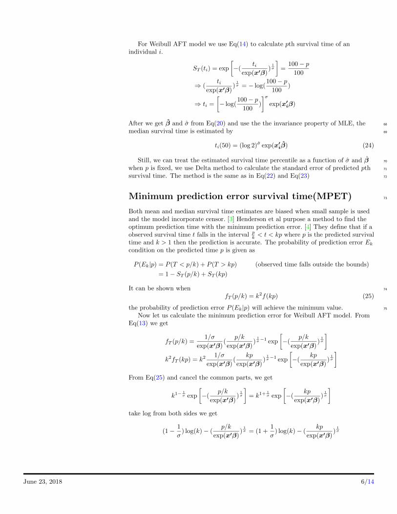
For Weibull AFT model we use Eq(14) to calculate pth survival time of anindividual i.

ST (ti) = exp

[−(

tiexp(x′β)

)1σ

]=

100− p100

⇒ (ti

exp(x′β))

1σ = − log(

100− p100

)

⇒ ti =

[− log(

100− p100

)

]σexp(x′

iβ)

After we get β̂ and σ̂ from Eq(20) and use the the invariance property of MLE, the 68

median survival time is estimated by 69

ti(50) = (log 2)σ̂ exp(x′iβ̂) (24)

Still, we can treat the estimated survival time percentile as a function of σ̂ and β̂ 70

when p is fixed, we use Delta method to calculate the standard error of predicted pth 71

survival time. The method is the same as in Eq(22) and Eq(23) 72

Minimum prediction error survival time(MPET) 73

Both mean and median survival time estimates are biased when small sample is usedand the model incorporate censor. [3] Henderson et al purpose a method to find theoptimum prediction time with the minimum prediction error. [4] They define that if aobserved survival time t falls in the interval pk < t < kp where p is the predicted survivaltime and k > 1 then the prediction is accurate. The probability of prediction error Ekcondition on the predicted time p is given as

P (Ek|p) = P (T < p/k) + P (T > kp) (observed time falls outside the bounds)

= 1− ST (p/k) + ST (kp)

It can be shown when 74

fT (p/k) = k2f(kp) (25)

the probability of prediction error P (Ek|p) will achieve the minimum value. 75

Now let us calculate the minimum prediction error for Weibull AFT model. FromEq(13) we get

fT (p/k) =1/σ

exp(x′β)(

p/k

exp(x′β))

1σ−1 exp

[−(

p/k

exp(x′β))

1σ

]k2fT (kp) = k2

1/σ

exp(x′β)(

kp

exp(x′β))

1σ−1 exp

[−(

kp

exp(x′β))

1σ

]From Eq(25) and cancel the common parts, we get

k1−1σ exp

[−(

p/k

exp(x′β))

1σ

]= k1+

1σ exp

[−(

kp

exp(x′β))

1σ

]take log from both sides we get

(1− 1

σ) log(k)− (

p/k

exp(x′β))

1σ = (1 +

1

σ) log(k)− (

kp

exp(x′β))

1σ

June 23, 2018 6/14

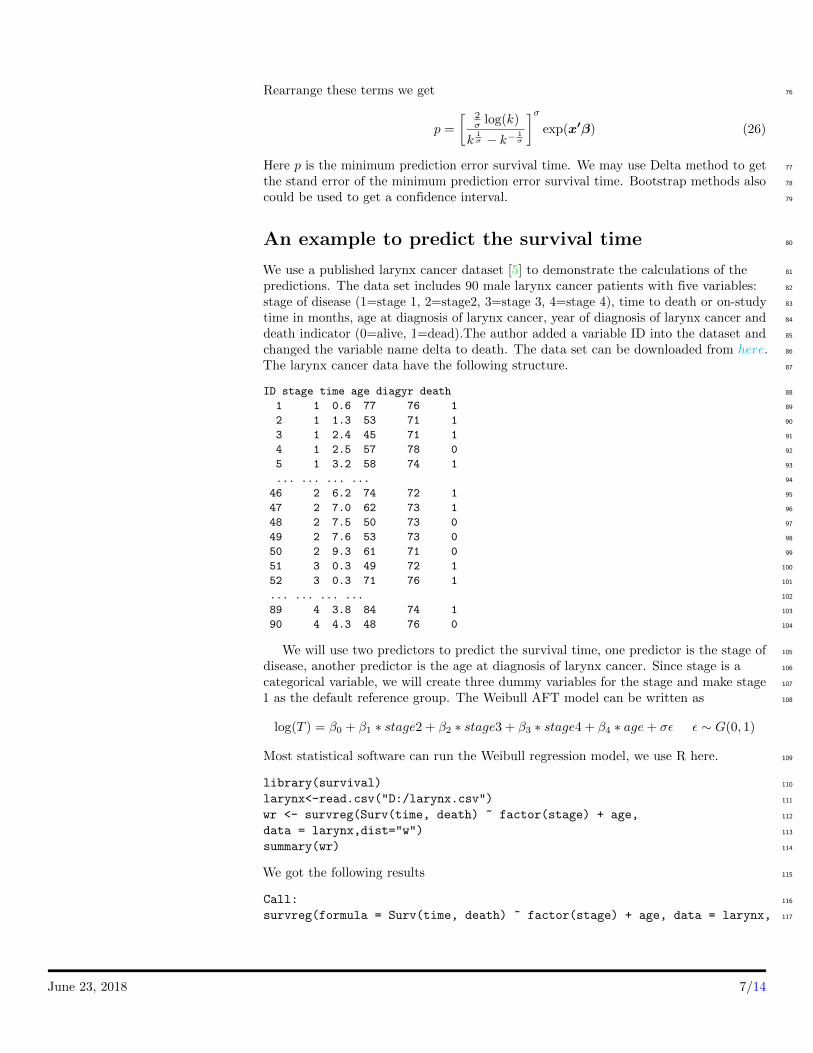
Rearrange these terms we get 76

p =

[ 2σ log(k)

k1σ − k− 1

σ

]σexp(x′β) (26)

Here p is the minimum prediction error survival time. We may use Delta method to get 77

the stand error of the minimum prediction error survival time. Bootstrap methods also 78

could be used to get a confidence interval. 79

An example to predict the survival time 80

We use a published larynx cancer dataset [5] to demonstrate the calculations of the 81

predictions. The data set includes 90 male larynx cancer patients with five variables: 82

stage of disease (1=stage 1, 2=stage2, 3=stage 3, 4=stage 4), time to death or on-study 83

time in months, age at diagnosis of larynx cancer, year of diagnosis of larynx cancer and 84

death indicator (0=alive, 1=dead).The author added a variable ID into the dataset and 85

changed the variable name delta to death. The data set can be downloaded from here. 86

The larynx cancer data have the following structure. 87

ID stage time age diagyr death 88

1 1 0.6 77 76 1 89

2 1 1.3 53 71 1 90

3 1 2.4 45 71 1 91

4 1 2.5 57 78 0 92

5 1 3.2 58 74 1 93

... ... ... ... 94

46 2 6.2 74 72 1 95

47 2 7.0 62 73 1 96

48 2 7.5 50 73 0 97

49 2 7.6 53 73 0 98

50 2 9.3 61 71 0 99

51 3 0.3 49 72 1 100

52 3 0.3 71 76 1 101

... ... ... ... 102

89 4 3.8 84 74 1 103

90 4 4.3 48 76 0 104

We will use two predictors to predict the survival time, one predictor is the stage of 105

disease, another predictor is the age at diagnosis of larynx cancer. Since stage is a 106

categorical variable, we will create three dummy variables for the stage and make stage 107

1 as the default reference group. The Weibull AFT model can be written as 108

log(T ) = β0 + β1 ∗ stage2 + β2 ∗ stage3 + β3 ∗ stage4 + β4 ∗ age+ σε ε ∼ G(0, 1)

Most statistical software can run the Weibull regression model, we use R here. 109

library(survival) 110

larynx<-read.csv("D:/larynx.csv") 111

wr <- survreg(Surv(time, death) ~ factor(stage) + age, 112

data = larynx,dist="w") 113

summary(wr) 114

We got the following results 115

Call: 116

survreg(formula = Surv(time, death) ~ factor(stage) + age, data = larynx, 117

June 23, 2018 7/14

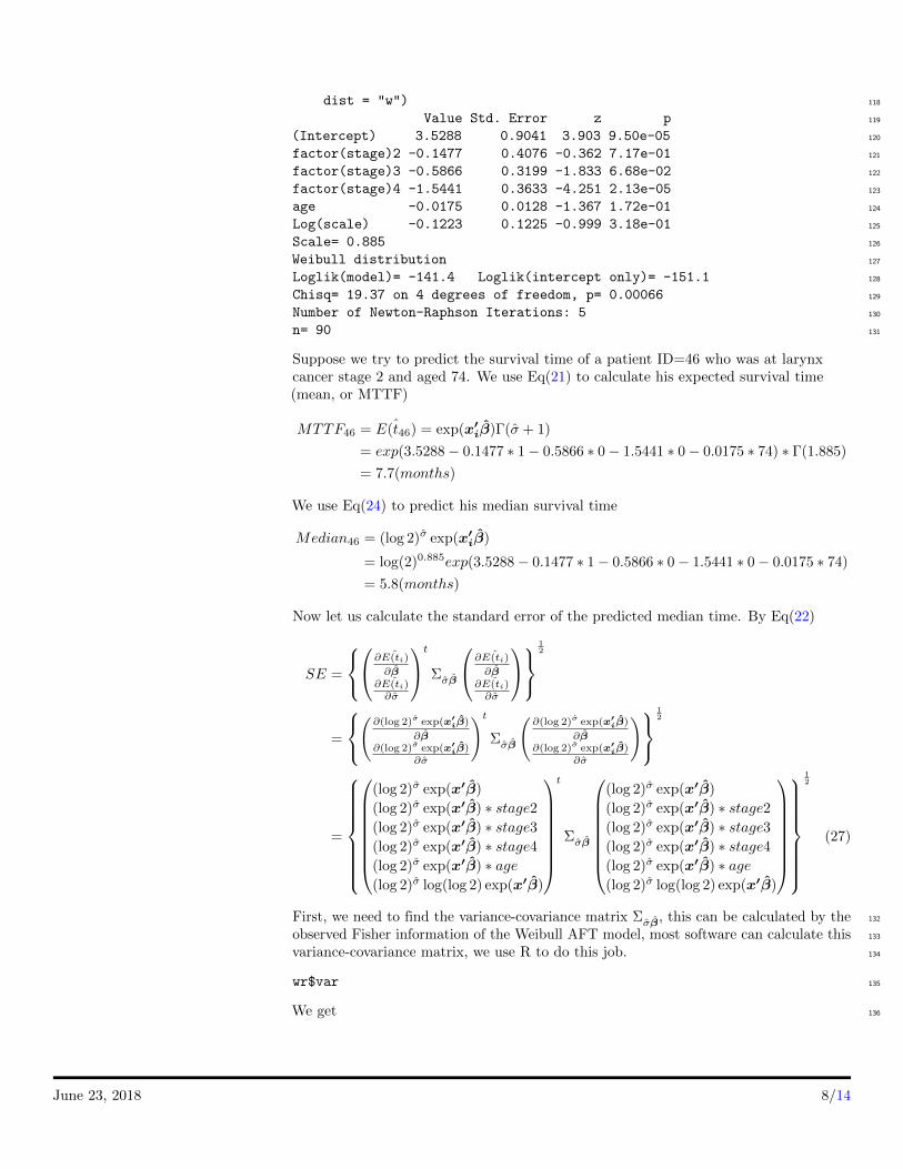
dist = "w") 118

Value Std. Error z p 119

(Intercept) 3.5288 0.9041 3.903 9.50e-05 120

factor(stage)2 -0.1477 0.4076 -0.362 7.17e-01 121

factor(stage)3 -0.5866 0.3199 -1.833 6.68e-02 122

factor(stage)4 -1.5441 0.3633 -4.251 2.13e-05 123

age -0.0175 0.0128 -1.367 1.72e-01 124

Log(scale) -0.1223 0.1225 -0.999 3.18e-01 125

Scale= 0.885 126

Weibull distribution 127

Loglik(model)= -141.4 Loglik(intercept only)= -151.1 128

Chisq= 19.37 on 4 degrees of freedom, p= 0.00066 129

Number of Newton-Raphson Iterations: 5 130

n= 90 131

Suppose we try to predict the survival time of a patient ID=46 who was at larynxcancer stage 2 and aged 74. We use Eq(21) to calculate his expected survival time(mean, or MTTF)

MTTF46 = ˆE(t46) = exp(x′iβ̂)Γ(σ̂ + 1)

= exp(3.5288− 0.1477 ∗ 1− 0.5866 ∗ 0− 1.5441 ∗ 0− 0.0175 ∗ 74) ∗ Γ(1.885)

= 7.7(months)

We use Eq(24) to predict his median survival time

Median46 = (log 2)σ̂ exp(x′iβ̂)

= log(2)0.885exp(3.5288− 0.1477 ∗ 1− 0.5866 ∗ 0− 1.5441 ∗ 0− 0.0175 ∗ 74)

= 5.8(months)

Now let us calculate the standard error of the predicted median time. By Eq(22)

SE =

∂ ˆE(ti)

∂β̂∂ ˆE(ti)∂σ̂

t

Σσ̂β̂

∂ ˆE(ti)

∂β̂∂ ˆE(ti)∂σ̂

12

=

(∂(log 2)σ̂ exp(x′

iβ̂)

∂β̂∂(log 2)σ̂ exp(x′

iβ̂)∂σ̂

)tΣσ̂β̂

(∂(log 2)σ̂ exp(x′

iβ̂)

∂β̂∂(log 2)σ̂ exp(x′

iβ̂)∂σ̂

)12

=

(log 2)σ̂ exp(x′β̂)

(log 2)σ̂ exp(x′β̂) ∗ stage2(log 2)σ̂ exp(x′β̂) ∗ stage3(log 2)σ̂ exp(x′β̂) ∗ stage4(log 2)σ̂ exp(x′β̂) ∗ age(log 2)σ̂ log(log 2) exp(x′β̂)

t

Σσ̂β̂

(log 2)σ̂ exp(x′β̂)

(log 2)σ̂ exp(x′β̂) ∗ stage2(log 2)σ̂ exp(x′β̂) ∗ stage3(log 2)σ̂ exp(x′β̂) ∗ stage4(log 2)σ̂ exp(x′β̂) ∗ age(log 2)σ̂ log(log 2) exp(x′β̂)

12

(27)

First, we need to find the variance-covariance matrix Σσ̂β̂, this can be calculated by the 132

observed Fisher information of the Weibull AFT model, most software can calculate this 133

variance-covariance matrix, we use R to do this job. 134

wr$var 135

We get 136

June 23, 2018 8/14

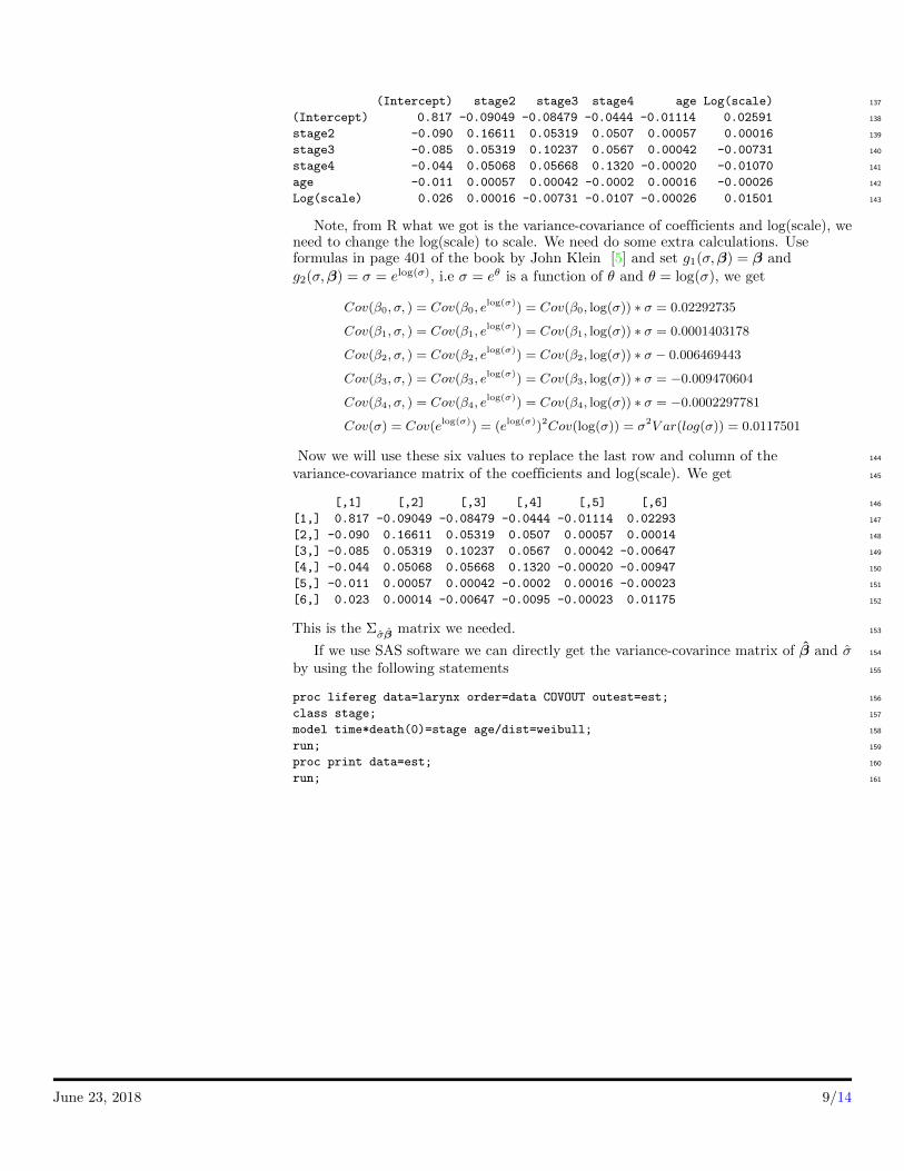
(Intercept) stage2 stage3 stage4 age Log(scale) 137

(Intercept) 0.817 -0.09049 -0.08479 -0.0444 -0.01114 0.02591 138

stage2 -0.090 0.16611 0.05319 0.0507 0.00057 0.00016 139

stage3 -0.085 0.05319 0.10237 0.0567 0.00042 -0.00731 140

stage4 -0.044 0.05068 0.05668 0.1320 -0.00020 -0.01070 141

age -0.011 0.00057 0.00042 -0.0002 0.00016 -0.00026 142

Log(scale) 0.026 0.00016 -0.00731 -0.0107 -0.00026 0.01501 143

Note, from R what we got is the variance-covariance of coefficients and log(scale), weneed to change the log(scale) to scale. We need do some extra calculations. Useformulas in page 401 of the book by John Klein [5] and set g1(σ,β) = β andg2(σ,β) = σ = elog(σ), i.e σ = eθ is a function of θ and θ = log(σ), we get

Cov(β0, σ, ) = Cov(β0, elog(σ)) = Cov(β0, log(σ)) ∗ σ = 0.02292735

Cov(β1, σ, ) = Cov(β1, elog(σ)) = Cov(β1, log(σ)) ∗ σ = 0.0001403178

Cov(β2, σ, ) = Cov(β2, elog(σ)) = Cov(β2, log(σ)) ∗ σ − 0.006469443

Cov(β3, σ, ) = Cov(β3, elog(σ)) = Cov(β3, log(σ)) ∗ σ = −0.009470604

Cov(β4, σ, ) = Cov(β4, elog(σ)) = Cov(β4, log(σ)) ∗ σ = −0.0002297781

Cov(σ) = Cov(elog(σ)) = (elog(σ))2Cov(log(σ)) = σ2V ar(log(σ)) = 0.0117501

Now we will use these six values to replace the last row and column of the 144

variance-covariance matrix of the coefficients and log(scale). We get 145

[,1] [,2] [,3] [,4] [,5] [,6] 146

[1,] 0.817 -0.09049 -0.08479 -0.0444 -0.01114 0.02293 147

[2,] -0.090 0.16611 0.05319 0.0507 0.00057 0.00014 148

[3,] -0.085 0.05319 0.10237 0.0567 0.00042 -0.00647 149

[4,] -0.044 0.05068 0.05668 0.1320 -0.00020 -0.00947 150

[5,] -0.011 0.00057 0.00042 -0.0002 0.00016 -0.00023 151

[6,] 0.023 0.00014 -0.00647 -0.0095 -0.00023 0.01175 152

This is the Σσ̂β̂ matrix we needed. 153

If we use SAS software we can directly get the variance-covarince matrix of β̂ and σ̂ 154

by using the following statements 155

proc lifereg data=larynx order=data COVOUT outest=est; 156

class stage; 157

model time*death(0)=stage age/dist=weibull; 158

run; 159

proc print data=est; 160

run; 161

June 23, 2018 9/14

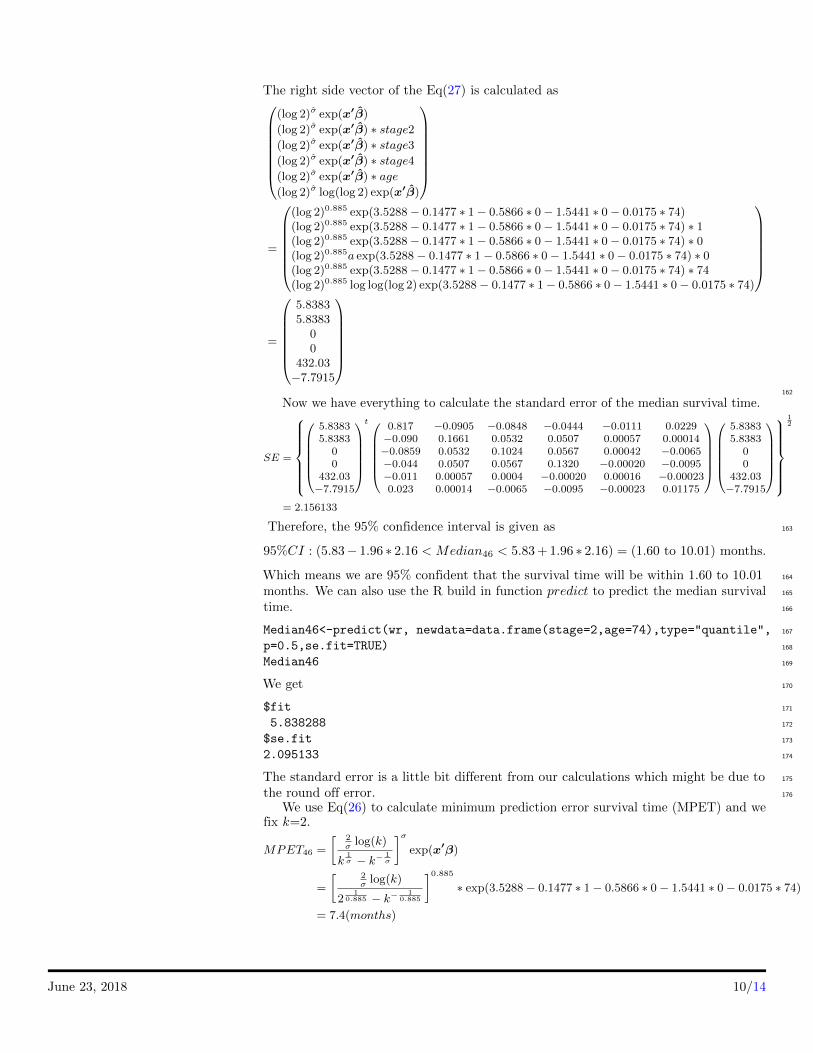
The right side vector of the Eq(27) is calculated as

(log 2)σ̂ exp(x′β̂)

(log 2)σ̂ exp(x′β̂) ∗ stage2(log 2)σ̂ exp(x′β̂) ∗ stage3(log 2)σ̂ exp(x′β̂) ∗ stage4(log 2)σ̂ exp(x′β̂) ∗ age(log 2)σ̂ log(log 2) exp(x′β̂)

=

(log 2)0.885 exp(3.5288− 0.1477 ∗ 1− 0.5866 ∗ 0− 1.5441 ∗ 0− 0.0175 ∗ 74)(log 2)0.885 exp(3.5288− 0.1477 ∗ 1− 0.5866 ∗ 0− 1.5441 ∗ 0− 0.0175 ∗ 74) ∗ 1(log 2)0.885 exp(3.5288− 0.1477 ∗ 1− 0.5866 ∗ 0− 1.5441 ∗ 0− 0.0175 ∗ 74) ∗ 0(log 2)0.885a exp(3.5288− 0.1477 ∗ 1− 0.5866 ∗ 0− 1.5441 ∗ 0− 0.0175 ∗ 74) ∗ 0(log 2)0.885 exp(3.5288− 0.1477 ∗ 1− 0.5866 ∗ 0− 1.5441 ∗ 0− 0.0175 ∗ 74) ∗ 74(log 2)0.885 log log(log 2) exp(3.5288− 0.1477 ∗ 1− 0.5866 ∗ 0− 1.5441 ∗ 0− 0.0175 ∗ 74)

=

5.83835.8383

00

432.03−7.7915

162

Now we have everything to calculate the standard error of the median survival time.

SE =

5.83835.8383

00

432.03−7.7915

t0.817 −0.0905 −0.0848 −0.0444 −0.0111 0.0229−0.090 0.1661 0.0532 0.0507 0.00057 0.00014−0.0859 0.0532 0.1024 0.0567 0.00042 −0.0065−0.044 0.0507 0.0567 0.1320 −0.00020 −0.0095−0.011 0.00057 0.0004 −0.00020 0.00016 −0.000230.023 0.00014 −0.0065 −0.0095 −0.00023 0.01175

5.83835.8383

00

432.03−7.7915

12

= 2.156133

Therefore, the 95% confidence interval is given as 163

95%CI : (5.83− 1.96 ∗ 2.16 < Median46 < 5.83 + 1.96 ∗ 2.16) = (1.60 to 10.01) months.

Which means we are 95% confident that the survival time will be within 1.60 to 10.01 164

months. We can also use the R build in function predict to predict the median survival 165

time. 166

Median46<-predict(wr, newdata=data.frame(stage=2,age=74),type="quantile", 167

p=0.5,se.fit=TRUE) 168

Median46 169

We get 170

$fit 171

5.838288 172

$se.fit 173

2.095133 174

The standard error is a little bit different from our calculations which might be due to 175

the round off error. 176

We use Eq(26) to calculate minimum prediction error survival time (MPET) and wefix k=2.

MPET46 =

[ 2σlog(k)

k1σ − k−

1σ

]σexp(x′β)

=

[ 2σlog(k)

21

0.885 − k−1

0.885

]0.885∗ exp(3.5288− 0.1477 ∗ 1− 0.5866 ∗ 0− 1.5441 ∗ 0− 0.0175 ∗ 74)

= 7.4(months)

June 23, 2018 10/14

It seems the three prediction methods are all quite close to the real survival time of the 177

patient ID=46 which was 6.2 months. 178

Note in R build in predict function for Weibull AFT model type= ”response” 179

calculates exp(x′β̂) without the Γ(1 + σ̂) and type=”lp” calculates x′β̂ only, we should 180

not use them to predict MTTF. There is no software to calculate the minimum 181

prediction error survival time. 182

Assess the point prediction accuracy 183

Parkes [6] suggested a simple method to measure the accuracy of the predicted survival 184

time. Let t be the observed survival time and p is the predicted time, if p/k ≤ t ≤ kp 185

then the point prediction p is defined as ”accurate”, outside the interval is defined as” 186

inaccurate”. Christakis and Lamont purposed a 33 percent rule to measure the 187

accuracy, where they divided the observed time by the predicted survival time, and 188

defined the prediction is “accurate” if this quotient was between 0.67 and 1.33. Values 189

less than 0.67 or greater than 1.33 were defined as “error”. [7] This method in fact is 190

just fix k = 3 in Parkes’ method. We choose k = 2 for our accuracy assessment. The 191

accurate rate is defined as the proportion of ”accurate” prediction over the total sample 192

size. The results were presented in table 1. 193

Discussion 194

In this paper, we introduced how to use Weibull AFT model to predict survival times. 195

Mean survival time (mean time to failure time, mean time between failures), median 196

survival time and minimum prediction error survival time were used to predict the 197

survival time and the prediction accuracy was assessed by Parke’s method. When we 198

fixed k = 2 the accuracy was 55.6% for median, 50% for MTTF and 51.1% for MPET. 199

If we fixed k = 3 as suggested by Christakis and Lamont the accuracy rate was 200

increased to 77.8%,66.7 % and 67.8%, respectively. The sample we used is quite small 201

and we only used two predictors, with bigger sample size and more predictors the 202

accuracy rate might be even higher. In this sample we did not observe that minimum 203

prediction error time had better accuracy rate than median survival time. 204

The parametric survival models have advantages in predicting survival time than the 205

semi-parametric Cox regression model. The Cox regression model which can be 206

specified as Si(t|xi) = S0(t)exp(x′iβ) cannot predict time directly. What it can do is to 207

specify a certain time first then to calculate the probability for that period of time. The 208

disadvantage of the parametric survival models is that we have to make stronger 209

assumptions than semi-parametric models. [8] 210

Currently, most clinical prediction models calculate a patient’s probability of having 211

or developing a certain disease or risk scores that based on the calculated 212

probabilities. [9]However, provide a probability seems difficult to be understand by 213

general population and probability itself can be defined by quite different ways. [10] In 214

practice, the time axis remains the most natural measure for both clinicians and patients. 215

It is much easier to understand a survival time rather than a subjective assessment of 216

probability of survival to a certain time point. [4] Predicting survival time can provide a 217

practical and concrete guide to clinicians and health care providers to manage their 218

patients and help families and patients make suitable plans for the remaining lifespan. 219

References

1. Gorgoso-Varela JJ, Rojo-Alboreca A. Use of Gumbel and Weibull functions tomodel extreme values of diameter distributions in forest stands. Annals of forest

June 23, 2018 11/14

science. 2014;71(7):741-50.

2. Lai C-D. Generalized Weibull Distributions. Generalized Weibull Distributions:Springer; 2014. p. 23-75.

3. Ho L, Silva A. Unbiased estimators for mean time to failure and percentiles in aWeibull regression model. International Journal of Quality & ReliabilityManagement.2006;23(3):323-39.

4. Henderson R, Jones M, Stare J. Accuracy of point predictions in survivalanalysis. Statistics in medicine. 2001;20(20):3083-96.

5. Klein JP, Moeschberger ML. Survival analysis: techniques for censored andtruncated data. Springer Science & Business Media; 2005.

6. Parkes CM. Accuracy of predictions of survival in later stages of cancer. Britishmedical journal. 1972;2(5804):29.

7. Christakis NA, Smith JL, Parkes CM, Lamont EB. Extent and determinants oferror in doctors’ prognoses in terminally ill patients: prospective cohortstudyCommentary: Why do doctors overestimate? Commentary: Prognosesshould be based on proved indices not intuition. Bmj. 2000;320(7233):469-73.

8. Nardi A, Schemper M. Comparing Cox and parametric models in clinical studies.Statistics in medicine. 2003;22(23):3597-610.

9. Lee Y-h, Bang H, Kim DJ. How to establish clinical prediction models.Endocrinology and Metabolism. 2016;31(1):38-44.

10. Saunders S. What is probability? Quo vadis quantum mechanics? Springer; 2005.p. 209-38.

June 23, 2018 12/14

Table 1. Prediction results and accuracy (last digit in predicted time: 0 inaccurate, 1,accurate)

ID stage age death time Median(95% CI) MTTF MPET1 1 77 1 0.6 6.42(3.16,9.68),0 8.47,0 8.11,02 1 53 1 1.3 9.77(4.07,15.46),0 12.9,0 12.34,03 1 45 1 2.4 11.23(3.07,19.39),0 14.84,0 14.19,04 1 57 0 2.5 9.11(4.32,13.89),0 12.03,0 11.5,05 1 58 1 3.2 8.95(4.36,13.54),0 11.82,0 11.3,06 1 51 0 3.2 10.11(3.88,16.34),0 13.36,0 12.78,07 1 76 1 3.3 6.54(3.29,9.78),1 8.62,0 8.25,08 1 63 0 3.3 8.2(4.37,12.03),0 10.83,0 10.36,09 1 43 1 3.5 11.63(2.72,20.54),0 15.36,0 14.7,010 1 60 1 3.5 8.64(4.4,12.89),0 11.41,0 10.91,011 1 52 1 4 9.94(3.98,15.89),0 13.13,0 12.55,012 1 63 1 4 8.2(4.37,12.03),0 10.83,0 10.36,013 1 86 1 4.3 5.49(1.96,9.01),1 7.24,1 6.92,114 1 48 0 4.5 10.66(3.52,17.79),0 14.08,0 13.47,015 1 68 0 4.5 7.52(4.12,10.91),1 9.92,0 9.49,016 1 81 1 5.3 5.99(2.63,9.34),1 7.9,1 7.56,117 1 70 0 5.5 7.26(3.96,10.56),1 9.58,1 9.16,118 1 58 0 5.9 8.95(4.36,13.54),1 11.82,0 11.3,119 1 47 0 5.9 10.84(3.38,18.31),1 14.33,0 13.7,020 1 75 1 6 6.65(3.41,9.89),1 8.78,1 8.39,121 1 77 0 6.1 6.42(3.16,9.68),1 8.47,1 8.11,122 1 64 0 6.2 8.06(4.34,11.77),1 10.64,1 10.18,123 1 77 1 6.4 6.42(3.16,9.68),1 8.47,1 8.11,124 1 67 1 6.5 7.65(4.19,11.1),1 10.1,1 9.66,125 1 79 0 6.5 6.2(2.9,9.5),1 8.18,1 7.83,126 1 61 0 6.7 8.49(4.4,12.58),1 11.21,1 10.73,127 1 66 0 7 7.78(4.25,11.31),1 10.27,1 9.83,128 1 68 1 7.4 7.52(4.12,10.91),1 9.92,1 9.49,129 1 73 0 7.4 6.89(3.65,10.12),1 9.09,1 8.69,130 1 56 0 8.1 9.27(4.28,14.26),1 12.24,1 11.71,131 1 73 0 8.1 6.89(3.65,10.12),1 9.09,1 8.69,132 1 58 0 9.6 8.95(4.36,13.54),1 11.82,1 11.3,133 1 68 0 10.7 7.52(4.12,10.91),1 9.92,1 9.49,134 2 86 1 0.2 4.73(0.68,8.78),0 6.25,0 5.97,035 2 64 1 1.8 6.95(2.37,11.54),0 9.18,0 8.78,036 2 63 1 2 7.07(2.4,11.75),0 9.34,0 8.93,037 2 71 0 2.2 6.15(1.96,10.34),0 8.12,0 7.77,038 2 67 0 2.6 6.6(2.22,10.97),0 8.71,0 8.33,039 2 51 0 3.3 8.72(2.28,15.17),0 11.52,0 11.02,040 2 70 1 3.6 6.26(2.03,10.49),1 8.26,0 7.9,041 2 72 0 3.6 6.05(1.89,10.2),1 7.98,0 7.63,042 2 81 1 4 5.17(1.13,9.21),1 6.82,1 6.52,143 2 47 0 4.3 9.36(1.98,16.73),0 12.36,0 11.82,044 2 64 0 4.3 6.95(2.37,11.54),1 9.18,0 8.78,045 2 66 0 5 6.71(2.28,11.15),1 8.86,1 8.48,1

June 23, 2018 13/14

Table 1 continued Prediction results and accuracy (last digit in predicted time: 0inaccurate, 1, accurate)

ID stage age death time Median(95% CI) MTTF MPET46 2 74 1 6.2 5.84(1.73,9.94),1 7.7,1 7.37,147 2 62 1 7 7.2(2.43,11.97),1 9.51,1 9.09,148 2 50 0 7.5 8.88(2.22,15.54),1 11.73,1 11.22,149 2 53 0 7.6 8.42(2.38,14.47),1 11.13,1 10.64,150 2 61 0 9.3 7.33(2.46,12.2),1 9.67,1 9.25,151 3 49 1 0.3 5.83(2.41,9.24),0 7.69,0 7.36,052 3 71 1 0.3 3.97(2.19,5.75),0 5.24,0 5.01,053 3 57 1 0.5 5.07(2.68,7.45),0 6.69,0 6.4,054 3 79 1 0.7 3.45(1.56,5.34),0 4.55,0 4.35,055 3 82 1 0.8 3.27(1.32,5.23),0 4.32,0 4.13,056 3 49 1 1 5.83(2.41,9.24),0 7.69,0 7.36,057 3 60 1 1.3 4.81(2.68,6.94),0 6.35,0 6.07,058 3 64 1 1.6 4.48(2.58,6.39),0 5.92,0 5.66,059 3 74 1 1.8 3.76(1.96,5.56),0 4.97,0 4.75,060 3 72 1 1.9 3.9(2.12,5.68),0 5.14,0 4.92,061 3 53 1 1.9 5.43(2.6,8.27),0 7.17,0 6.86,062 3 54 1 3.2 5.34(2.63,8.05),1 7.05,0 6.74,063 3 81 1 3.5 3.33(1.4,5.27),1 4.39,1 4.2,164 3 52 0 3.7 5.53(2.56,8.49),1 7.3,1 6.98,165 3 66 0 4.5 4.33(2.49,6.17),1 5.71,1 5.47,166 3 54 0 4.8 5.34(2.63,8.05),1 7.05,1 6.74,167 3 63 0 4.8 4.56(2.61,6.51),1 6.02,1 5.76,168 3 59 1 5 4.89(2.69,7.1),1 6.46,1 6.18,169 3 49 0 5 5.83(2.41,9.24),1 7.69,1 7.36,170 3 69 0 5.1 4.11(2.32,5.89),1 5.42,1 5.19,171 3 70 1 6.3 4.04(2.26,5.82),1 5.33,1 5.1,172 3 65 1 6.4 4.41(2.54,6.27),1 5.82,1 5.56,173 3 65 0 6.5 4.41(2.54,6.27),1 5.82,1 5.56,174 3 68 1 7.8 4.18(2.38,5.98),1 5.52,1 5.28,175 3 78 0 8 3.51(1.64,5.38),0 4.63,1 4.43,176 3 69 0 9.3 4.11(2.32,5.89),0 5.42,1 5.19,177 3 51 0 10.1 5.63(2.52,8.73),1 7.43,1 7.11,178 4 65 1 0.1 1.69(0.77,2.61),0 2.23,0 2.14,079 4 71 1 0.3 1.52(0.7,2.34),0 2.01,0 1.92,080 4 76 1 0.4 1.4(0.61,2.18),0 1.84,0 1.76,081 4 65 1 0.8 1.69(0.77,2.61),0 2.23,0 2.14,082 4 78 1 0.8 1.35(0.56,2.13),1 1.78,0 1.7,083 4 41 1 1 2.57(0.3,4.84),0 3.4,0 3.25,084 4 68 1 1.5 1.6(0.74,2.47),1 2.12,1 2.03,185 4 69 1 2 1.58(0.73,2.42),1 2.08,1 1.99,186 4 62 1 2.3 1.78(0.78,2.79),1 2.35,1 2.25,187 4 74 0 2.9 1.44(0.65,2.24),0 1.91,1 1.82,188 4 71 1 3.6 1.52(0.7,2.34),0 2.01,1 1.92,189 4 84 1 3.8 1.21(0.42,2.01),0 1.6,0 1.53,090 4 48 0 4.3 2.28(0.57,3.99),1 3.01,1 2.87,1Accuracy rate(%) 55.6%(50/90) 50%(45/90) 51.1%(46/90)

June 23, 2018 14/14