USITC Analysis of Trade Policy IssuesPresentation at the Ministry of Commerce

Beijing, China, October 23, 2006 Bob Koopman, Chief Economist

Director, Office of Economics

United States International Trade Commission

These remarks are my own and do not necessarily reflect the views of the USITC or any of its individual Commissioners.

Overview of seminar• Provide an overview of:

– some of the questions we address and the economic models used at the USITC to analyze trade policy issues.

– how the ITC’s work is used in U.S. trade policy formulation and deliberation.

– ITC is an independent agency not part of Presidential Administration. (See HSE presentation for more on this.)

– ITC operates under a number of specific statutes or laws• Sections 131, 332, 2104,etc. of various trade acts – 1974, 2002

• Office of Economics has approximately 48 staff, some visiting scholars. Very few support staff – research assistants. Mostly PhDs, but some masters and ABDs. – ITC staff level is 350, Office of Industries (partner office on most

studies) has approximately 100 staff.• USITC’s independence is important and one of its most

valued assets along with its employees.

USITC continued• USITC had five main areas of responsibility

– Import injury work• AD/CVD and Safeguard

– Intellectual property rights• “337” cases

– Industry and Economic Analysis• Studies on FTA’s, and other trade related topics

– Maintaining the US Tariff– Providing informal assistance based on our expertise to USTR

and Congress as requested on trade related matters• USITC holds public hearings, writes both public and non

public reports, and provides a venue for interested parties to report their concerns over policy issues.

• The ITC is viewed as independent and objective in its analysis.

Trade Policy Development in the United States – the Policy Process

• Roles of Congress and the President defined by the U.S. Constitution and subsequent legislation– Congress given authority over trade– But through many years of legislation

Congress has given the President much discretion and authority over negotiations, while retaining responsibility for final approval.

Congress

• Congressional authority over trade defined under Article 1, Section 8 of the Constitution – known as the Commerce Clause– grants the Congress the right to "regulate

commerce with foreign nations, and among the several States,"

Congress and Trade• Congress has 2 houses, the House of Representatives and the

Senate.• 2 Congressional Committees largely responsible for, among other

things, trade issues – House Committee on Ways and Means– Senate Finance Committee– Both are important and influential committees with wide ranging

responsibilities.– The USITC can be given work by either of these committees.

• Any member of Congress can introduce trade related legislation, but it is likely to be referred to one of these Committees for consideration. – If it doesn’t make it out of Committee, the legislation is dead.– Sometimes trade related legislation is added to other, non trade related

bills as amendments, and may by pass these committees, but that is rare.

Sources of input for Congressional Views on Trade

• Congress has numerous mechanisms for obtaining input on trade issues.– Constituent input– Public Hearings– Briefing by the President’s Administration, lobbyists,

public interest groups, etc.

President• The President has the right to make treaties

– “(the President)… shall have power, by and with the advice and consent of the Senate, to make treaties, provided two thirds of the Senators present concur; and he shall nominate, and by and with the advice and consent of the Senate”

• However, starting in 1934 Congress provided authority to the President to reduce tariffs through bilateral and GATT multilateral trade negotiations.– In 1962 Congress establishes USTR predecessor, and authorizes

President Kennedy to agree to up to 50% reductions in on most items in US tariff schedule on a reciprocal basis.

– 1974 Trade Act first time President given authority to negotiate non-tariff barriers and provides Fast Track Authority (for a period of 5 years), where Congress agrees to consider the trade agreements as presented by the administration without making amendments.

– Fast Track renewed in 1979, 1984, 1988 (8 months after expiration), 1991, and 1993. Not renewed at the end of 1994. 2002 Trade Act provides for Trade Promotion Authority (TPA) – Fast Track’s replacement. TPA expires June 2007.

President and Trade

• The United States Trade Representative is part of the Executive Office of the President and is delegated authority by the President to negotiate trade agreements.

• The President retains the decision making responsibility.

Where is the ITC in the policy process?

President

CEA DOA DOC DOD DOE HHS DOI DOJ DOL DOS DOT Treas. EPA AID NEC NSC OMB

Advisory Committees

USITC

Congress

House, Ways & Means Senate Finance Committee

CEQ

USTR and Trade Policy Staff Committee

Some analytical tools we use…• The USITC uses partial equilibrium and general

equilibrium simulation models, and econometric models to analyze trade measures. Will provide examples as we go.– PE models are largely commodity specific, Armington

specification, applied at 6 or 8 digit tariff line. Some multi sector PE models are used also.

– GE models include:• large scale, 500+ sector model of the U.S., United States Applied

General Equilibrium Model (USAGE).• Large scale world model, Global Trade Analysis Project (GTAP)

model (based at Purdue University.)– Econometric models applied recently include gravity models,

reduced form supply and demand models, logit and probit specifications.

• Choice of econometric specification depends very much on the question we are asked to answer.

Broad context for ITC analysis…• USITC analysis is used at many stages in the trade

policy formulation and deliberation process.– Our economic analysis, and that of others, NEVER determines

the policy choice. It is used as one input to the policy process.– ITC analysis is used before negotiations begin on FTAs (largely

commodity specific PE analysis.) – won’t provide examples but can discuss if you are interested.

– ITC analysis is used after negotiations are completed, but before Congressional vote on FTA (usually GE analysis for economywide effects and broad sectoral impacts.)

– ITC analysis is used to inform debate on many other topics• Significant U.S. import restraints and steel special safeguards –

(examples follow – large single country CGE model)• China’s accession to WTO and FTA’s (global CGE model)• Non-Tariff Measures

Example of independence

• Trade liberalization and growth– Policymakers (USTR) wanted to assert that trade

liberalization causes growth

• Asked ITC to prepare report that examined the theoretical and empirical research, summarized current findings, and recommended areas for further research.

Independence sometimes means not everyone agrees…

• Some Commissioners were skeptical that economic theory and empirical work could answer the question “correctly.”

Our answer was that trade liberalization and growth were not as directly linked as some had expected …

Recent summary from OECD Trade Committee summary - 2006

But we still get asked…some recent questions…

• Market for Medical Devices – Japan• HK – EBA• Asia trade patterns and FDI• Peru FTA, Colombia FTA, Ecuador FTA, etc…• South Korea and Malaysia probable economic

effects advice• We usually get 6 to 12 months to complete

studies, but FTA studies often done in 3 to 4 months

Economic Models used at the ITC• The USAGE model – developed jointly with Peter Dixon, COPS, Monash U.

– A dynamic, regional applied general equilibrium (AGE) model of the U.S. economy with capability to analyze effects for distinct labor and household categories

– 513 sectors, dynamic– Four closures

• Historical, decomposition, forecast, and policy• Calibrates the model more tightly to observed data over time

– Examines changes to parameters on tastes and technology – Helps identify areas in the data or model that need further attention

– Add-ons• Take AGE results as an input and produce results for variables not included in AGE

model• Offer computational advantages

– State-level effects – all 50 states - completed– Distinct labor categories with different economic characteristics – flexible, but up

to 753 occupations, self employment, and farming – in development– Distinct household categories with different primary factor endowments and

demands (BLS data from Current Household and Payroll Surveys) – again flexible, but probably no more than 10 – data gathering.

– Refinements• Sweetener markets – U.S. sugar policy – explicit modeling of US quotas using

complementarities.• Jones act, upcoming

USAGE• I’ll elaborate a bit on this model – will play important role

in our future work by addressing a number of concerns customers have raised about economic models in general.

• Model validity, dynamics, state level results, labor detail, and household breakouts

• Data source 1992 U.S. Input – Output table– Updated annually annual BLS 182 sector macro data and trade

data - currently to 2004.– Major new challenge – BEA changed from SIC to NAICs

classifications, most up-to-date IO table is in NAICs – 2002. We must redo all our data.

– Then projected to 2015 using “outside forecasts” for key macro variables and labor.

USAGE closures to ensure model fits historical data and official government forecasts

• We follow Australian Monash approach and use closures to “validate” the model on recent data and fit projections to official government forecasts – CBO, BLS, etc.

• Historical closure

– Estimating changes in tastes/technology, 1992-2001

• Decomposition closure – Decomposing effects of economic developments, 1992-2001– What were the effects of changing tastes and technologies versus observed changes in

policy variables.

• Forecasting (projection) closure– Projecting, 2001-15, annually – forms baseline consistent with government macro forecasts

• Policy closure– Policy analysis, 2001-15, annually – examines potential effects of policy changes as

deviations from baseline.

Historical simulation• An attempt to rectify problem of infrequent and outdated Input-Output (I-O)

tables– an attractive alternative to mechanical update methods such as RAS

• Historical simulation approach– Flexible approach regarding data requirements– Based on USAGE-ITC theory– By-product

• Detailed and interpretable estimates of changes in household preferences and industry technologies

• Central input to decomposition and forecast simulations

• By-product overshadows up-to-date I-O tables as the major output of historical simulation

• Done by swapping endogenous and exogenous variables in closure.

Naturally endogenous data, 2001e.g., Imports, exports by commodityEmployment and capital inputs by

industry

Historical closure, long run

Naturally exogenous data, 2001e.g., CIF import prices, foreign currency

Tariff rates Changes in tastes/technology, 1992-01e.g., Shifts in import/domestic preferences

Shifts in foreign demandPrimary-factor-saving technical change

and capital/labor bias in technical change

Historical simulation, 1992-2001

USAGE 1992

Naturally endogenous data, 2001

Historical closure

USAGE 1992

Naturally exogenous data, 2001

Decomposition closure

Decomposition of effects of trade policy

and technological change, 1992-2001

Changes in tastes & technology, 1992-01

Historical and decomposition simulations, 1992-2001

USAGE 1992

State-level add-on

State level decomposition

Percentage changes in employment

Percentage changes in output

No. Industry 92 to 98 98 to 04 92 to 98 98 to 04

244 SteelWire -1 -22 18 -2 245 SteelSheet -3 -31 19 -9 246 SteelPipe -1 -16 19 4 247 IronSteel 13 -30 27 -9 248 IronStlForg 31 -27 48 0

Example:Iron and Steel Employment and Output

Example:Iron and Steel, 1992-1998

1 2 3 4 5 6 7

Shifts in foreign demand & import prices

Changes in tariffs

Tech. change

Changes in import/

domestic preferences

Growth in employ-

ment

Apparent changes in profitability

Other factors

Total

1 Real GDP (gdp) 2.09 0.03 6.67 -0.64 13.53 -1.98 0.76

20.45

2 IS output – gdp -4.18 0.10 6.70 1.46 4.51 -1.26 -0.52 6.81 3 ISF output – gdp -5.21 0.12 22.31 2.63 6.00 -2.40 -2.88 20.59 4 IS users’ output – gdp -4.07 0.05 16.02 2.20 4.76 -1.25 1.24 18.95

5 ISF users’ output – gdp -5.29 0.11 20.92 2.78 5.67 -2.19 -2.79 19.23 6 Car parts output - gdp -4.48 0.07 21.16 5.85 7.22 12.37 -13.27 28.94 7 Int. c. eng. output - gdp -7.20 0.12 25.42 1.79 5.85 -11.64 -0.22 14.12 8 Real investment -gdp 3.56 0.09 -1.26 -0.41 0.51 -3.55 29.61 28.56

Annual forecast simulations, 2001-15

Annual forecasts: naturally exogenous & endogenous variables

• Macro

• Trade policy

• Exports, Imports

USAGE

Forecast closure, short run

Forecast paths

Shifts in functions (e.g., foreign demands,

export supplies) and macro coefficients,

e.g., APC

Changes in tastes & technologyindustry, commodity specific

The U.S. economy: 1992 to 2010percentage growth over 6-year periods

1992 to 1998 obs. 1998 to 2004 obs. 2004 to 2010 proj.

C 22.80 23.88 20.76

I 48.49 18.75 36.56

G 3.58 20.64 12.39

X 45.15 15.66 42.11

M 71.45 46.91 38.49

GDP 20.60 18.42 21.82

L 13.49 3.10 6.89

K 17.43 19.51 21.98

Total factor productivity 4.68 9.48 9.15

Exchange rate 13.40 -1.74 -13.59

Calculation of the current account deficit: 1992, 1998, 2004 and 2010 ($billion)

1992 1998 2004 2010 Imports 700 1155 1854 2847

- Exports -661 -991 -1191 -1895

Servicing of U.S. foreign liabilities 104 266 307 645

- Income from U.S. foreign assets -131 -267 -397 -877 Net transfers from U.S. to foreigners 35 48 72 116 Current account deficit (CAD) 48 211 645 836 CAD as percent of GDP 0.8 2.5 5.7 5.2

Annual forecast simulations• Contributes to generating believable AGE analysis

– “what if” answers depend significantly on the basecase forecast

• Incorporates detailed information from several expert groups (in our case official govt agency forecasts or projections.)

• USAGE-ITC forecasts/projections are of interest by themselves– Establishes a foreign trade baseline in some detail. Not a part

of original projections.

Annual forecast and policy simulations, 2001-15

Forecasts: naturally exog. & endogenous

• Macro

• Trade policy

• Exports, Imports

USAGE

Forecast closure Policy closure

Shocks: modified

forecasts for naturally

exogenous variables

Forecast paths

Shifts in functions

USAGE

Policy effects as deviations

from forecast

path

Policy paths

Δ tastes & technology

(iv) Conduct policy (or what if?) simulations as deviations from benchmark

• Import barriers • World trading conditions• Environmental constraints• Outsourcing• Homeland security, restrictions on foreign tourists and students• Homeland security, cargo inspections • Energy policies Important to obtain policy results as effects on the economy of a relevant future year, e.g. 2010 or 2020

Example:Iron and Steel, 1992-1998

1 2 3 4 5 6 7

Shifts in foreign demand & import prices

Changes in tariffs

Tech. change

Changes in import/

domestic preferences

Growth in employ-

ment

Apparent changes in profitability

Other factors

Total

1 Real GDP (gdp) 2.09 0.03 6.67 -0.64 13.53 -1.98 0.76

20.45

2 IS output – gdp -4.18 0.10 6.70 1.46 4.51 -1.26 -0.52 6.81 3 ISF output – gdp -5.21 0.12 22.31 2.63 6.00 -2.40 -2.88 20.59 4 IS users’ output – gdp -4.07 0.05 16.02 2.20 4.76 -1.25 1.24 18.95

5 ISF users’ output – gdp -5.29 0.11 20.92 2.78 5.67 -2.19 -2.79 19.23 6 Car parts output - gdp -4.48 0.07 21.16 5.85 7.22 12.37 -13.27 28.94 7 Int. c. eng. output - gdp -7.20 0.12 25.42 1.79 5.85 -11.64 -0.22 14.12 8 Real investment -gdp 3.56 0.09 -1.26 -0.41 0.51 -3.55 29.61 28.56

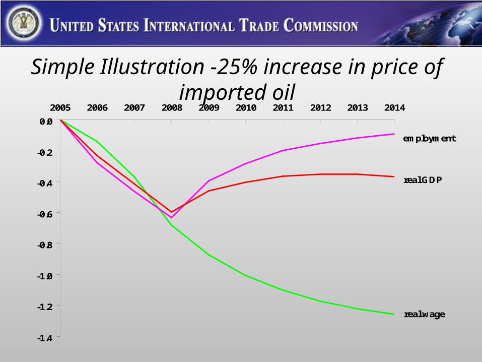
Simple Illustration -25% increase in price of imported oil

-1.4

-1.2

-1.0

-0.8

-0.6

-0.4

-0.2

0.0

2005 2006 2007 2008 2009 2010 2011 2012 2013 2014

real wage

employment

real GDP

25% increase in price of imported oil

-3.5

-3.0

-2.5

-2.0

-1.5

-1.0

-0.5

0.0

2005 2006 2007 2008 2009 2010 2011 2012 2013 2014

real GDP

investment

private consumption

imports

exports

25% increase in price of imported oil

-4

-2

0

2

4

6

8

10

12

14

2005 2006 2007 2008 2009 2010 2011 2012 2013 2014

Mining

Holiday

PetrolProds

Model validation in USAGE-ITC framework

• USAGE-ITC has most of requirements for statistically tested AGE forecasting model– Dynamic specification to allow forecasting to a year outside data– Fitting of historical events (historical simulations)– Incorporates detailed trend estimates of technology and

preferences

• But no statistical measure of validity – “estibration”, a combination of calibration and highly restricted estimation of select parameters with no statistical basis.

Example – Significant US Import Restraints– Used by USTR at WTO TPRM to demonstrate transparency re US import

restrictions– Significant tariffs and TRQs on food and agricultural products including canned

tuna, cotton, dairy products, peanuts, sugar and sugar-containing products, tobacco and tobacco products, beef, and ethyl alcohol;

– Significant tariffs as well as quotas on certain textiles and apparel pursuant to the Uruguay Round Agreement on Textiles and Clothing (ATC) and bilateral textile agreements with non-WTO member countries;

– Significant tariffs for a number of merchandise goods, including footwear and leather products; glass and glass products; watches, clocks, watch cases and parts; ball and roller bearings; ceramic wall and floor tile; table and kitchenware; costume jewelry; pens, mechanical pencils, and parts; and cutlery and hand tools.

– For 45 Input-Output industries we have calculated the percentage by which import restraints raise landed-duty-paid price.

– These percentages, which we refer to as wedges, are divided into two parts:• The first part is a tariff equivalent paid by importers, and• The second part is the increase in the price received by foreign suppliers

made possible by US-imposed quotas. This second part is often referred to as the export tax equivalent of the US quota regime ….

Price

Quantity of US imports

Q

PD

0

PM

Estimated price gap

SROW

SROW with export tax

DUSA

DUSA with import tariff

US import tariff equivalent

ROW export tax equivalent

Significant US import restraintsPrice gaps, US tariff equivalents, ROW export tax equivalent

0

10

20

30

40

50

60

70

80

90

100

110

Sugar

manufa

ctu

ring

Cre

am

ery

butter

Natu

ral,

pro

cessed, and im

itatio

n c

heese

Dry

, condensed, and e

vapora

ted d

airy p

roducts

Tobacco s

tem

min

g a

nd r

edry

ing

Ice c

ream

and fro

zen d

essert

s

Flu

id m

ilk

Oil

bearing c

rops

Cig

are

ttes

Canned a

nd c

ure

d fis

h a

nd s

eafo

ods

Meat packin

g p

lants

Appare

l made fro

m p

urc

hased m

ate

rials

Housefu

rnis

hin

gs, n.e

.c.

Curt

ain

s a

nd d

raperies

Bro

adw

oven fabric m

ills a

nd fabric fin

ishin

g p

lants

Knit

fabric m

ills

Hosie

ry, n.e

.c.

Thre

ad m

ills

Wom

en's

hosie

ry, except socks

Cellu

losic

manm

ade fib

ers

Canvas a

nd r

ela

ted p

roducts

Yarn

mills a

nd fin

ishin

g o

f te

xtil

es, n.e

.c.

Ple

atin

g a

nd s

titchin

g

Narr

ow

fabric m

ills

Cord

age a

nd tw

ine

Fabricate

d textil

e p

roducts

, n.e

.c.

Coate

d fabrics, not ru

bberized

Textil

e g

oods, n.e

.c.

Luggage

Leath

er

glo

ves a

nd m

ittens

Rubber

and p

lastic

s footw

ear

House s

lippers

Wom

en's

handbags a

nd p

urs

es

Shoes, except ru

bber

Pers

onal l

eath

er

goods, n.e

.c.

Vitr

eous c

hin

a table

and k

itchenw

are

Cera

mic

wall

and flo

or

tile

Costu

me je

welry

Ball

and r

olle

r bearings

Watc

hes, clo

cks, w

atc

hcases, and p

art

s

Fin

e e

art

henw

are

table

and k

itchenw

are

Pens, m

echanic

al p

encils

, and p

art

s

Gla

ss a

nd g

lass p

roducts

, except conta

iners

Cutle

ry

Hand a

nd e

dge tools

, except m

achin

e tools

and h

andsaw

s

US import tariff equivalent ROW export tax equivalent

Removal of significant US import restraintsPrice gaps and US output effects

-30

-20

-10

0

10

20

30

40

50

60

70

80

90

100

110

Sugar

manufa

ctu

ring

Cre

am

ery

butter

Natu

ral,

pro

cessed, and im

itatio

n c

heese

Dry

, condensed, and e

vapora

ted d

airy p

roducts

Tobacco s

tem

min

g a

nd r

edry

ing

Ice c

ream

and fro

zen d

essert

s

Flu

id m

ilk

Oil

bearing c

rops

Cig

are

ttes

Canned a

nd c

ure

d fis

h a

nd s

eafo

ods

Meat packin

g p

lants

Appare

l made fro

m p

urc

hased m

ate

rials

Housefu

rnis

hin

gs, n.e

.c.

Curt

ain

s a

nd d

raperies

Bro

adw

oven fabric m

ills a

nd fabric fin

ishin

g p

lants

Knit

fabric m

ills

Hosie

ry, n.e

.c.

Thre

ad m

ills

Wom

en's

hosie

ry, except socks

Cellu

losic

manm

ade fib

ers

Canvas a

nd r

ela

ted p

roducts

Yarn

mills a

nd fin

ishin

g o

f te

xtil

es, n.e

.c.

Ple

atin

g a

nd s

titchin

g

Narr

ow

fabric m

ills

Cord

age a

nd tw

ine

Fabricate

d textil

e p

roducts

, n.e

.c.

Coate

d fabrics, not ru

bberized

Textil

e g

oods, n.e

.c.

Luggage

Leath

er

glo

ves a

nd m

ittens

Rubber

and p

lastic

s footw

ear

House s

lippers

Wom

en's

handbags a

nd p

urs

es

Shoes, except ru

bber

Pers

onal l

eath

er

goods, n.e

.c.

Vitr

eous c

hin

a table

and k

itchenw

are

Cera

mic

wall

and flo

or

tile

Costu

me je

welry

Ball

and r

olle

r bearings

Watc

hes, clo

cks, w

atc

hcases, and p

art

s

Fin

e e

art

henw

are

table

and k

itchenw

are

Pens, m

echanic

al p

encils

, and p

art

s

Gla

ss a

nd g

lass p

roducts

, except conta

iners

Cutle

ry

Hand a

nd e

dge tools

, except m

achin

e tools

and h

andsaw

s

US price gap US output

Welfare impact of liberalization

Welfare changes from liberalization of all significant import restraints, by sector, million dollars, 2002

Sector

Change ineconomic

welfare

Simultaneous liberalization of all significant restraints. . . . . . . . . . . . . . . . . . . . . . . . . . . . . . . . . . . . . . . . . . . . . . 14,133

Individual liberalization: Textiles and apparel . . . . . . . . . . . . . . . . . . . . . . . . . . . . . . . . . . . . . . . . . . . . . . . . . . . . . . . . . . . . . . . . . . . . . . . . . . . . 11,759 Sugar . . . . . . . . . . . . . . . . . . . . . . . . . . . . . . . . . . . . . . . . . . . . . . . . . . . . . . . . . . . . . . . . . . . . . . . . . . . . . . . . . . . . . . . 1,089 Footwear and leather products . . . . . . . . . . . . . . . . . . . . . . . . . . . . . . . . . . . . . . . . . . . . . . . . . . . . . . . . . . . . . . . . . . 720 Tobacco and tobacco products . . . . . . . . . . . . . . . . . . . . . . . . . . . . . . . . . . . . . . . . . . . . . . . . . . . . . . . . . . . . . . . . . . . 145 Canned tuna . . . . . . . . . . . . . . . . . . . . . . . . . . . . . . . . . . . . . . . . . . . . . . . . . . . . . . . . . . . . . . . . . . . . . . . . . . . . . . . . . . 71 Beef. . . . . . . . . . . . . . . . . . . . . . . . . . . . . . . . . . . . . . . . . . . . . . . . . . . . . . . . . . . . . . . . . . . . . . . . . . . . . . . . . . . . . . . . . 66 Watches, clocks, watch cases and parts. . . . . . . . . . . . . . . . . . . . . . . . . . . . . . . . . . . . . . . . . . . . . . . . . . . . . . . . . . . . 65 Ball and roller bearings . . . . . . . . . . . . . . . . . . . . . . . . . . . . . . . . . . . . . . . . . . . . . . . . . . . . . . . . . . . . . . . . . . . . . . . . . 58 Ceramic wall and floor tile . . . . . . . . . . . . . . . . . . . . . . . . . . . . . . . . . . . . . . . . . . . . . . . . . . . . . . . . . . . . . . . . . . . . . . . 50 Dairy . . . . . . . . . . . . . . . . . . . . . . . . . . . . . . . . . . . . . . . . . . . . . . . . . . . . . . . . . . . . . . . . . . . . . . . . . . . . . . . . . . . . . . . . 30 Table and kitchenware . . . . . . . . . . . . . . . . . . . . . . . . . . . . . . . . . . . . . . . . . . . . . . . . . . . . . . . . . . . . . . . . . . . . . . . . . . 22 Costume jewelry. . . . . . . . . . . . . . . . . . . . . . . . . . . . . . . . . . . . . . . . . . . . . . . . . . . . . . . . . . . . . . . . . . . . . . . . . . . . . . . 22 Glass and glass products. . . . . . . . . . . . . . . . . . . . . . . . . . . . . . . . . . . . . . . . . . . . . . . . . . . . . . . . . . . . . . . . . . . . . . . . 8 Peanuts. . . . . . . . . . . . . . . . . . . . . . . . . . . . . . . . . . . . . . . . . . . . . . . . . . . . . . . . . . . . . . . . . . . . . . . . . . . . . . . . . . . . . . 6 Pens, mechanical pencils, and parts . . . . . . . . . . . . . . . . . . . . . . . . . . . . . . . . . . . . . . . . . . . . . . . . . . . . . . . . . . . . . . . 3 Cutlery and handtools. . . . . . . . . . . . . . . . . . . . . . . . . . . . . . . . . . . . . . . . . . . . . . . . . . . . . . . . . . . . . . . . . . . . . . . . . . . 1Source: USITC estimates.

Removal of significant US import restraintsGross State product effects, per cent

GSP GSP

33 North Carolina -0.685 51 Dist. Of Columbia 0.079

1 Alabama -0.420 46 Virginia 0.093

12 Idaho -0.381 44 Utah 0.119

40 South Carolina -0.350 43 Texas 0.127

39 Rhode Island -0.282 7 Connecticut 0.134

23 Minnesota -0.210 48 West Virginia 0.142

34 North Dakota -0.184 27 Nebraska 0.146

32 New York -0.166 13 Illinois 0.148

29 New Hampshire -0.154 8 Delaware 0.157

21 Massachusetts -0.134 31 New Mexico 0.158

30 New Jersey -0.123 36 Oklahoma 0.160

42 Tennessee -0.121 4 Arkansas 0.184

50 Wyoming -0.073 5 California 0.199

41 South Dakota -0.064 15 Iowa 0.209

18 Louisiana -0.047 20 Maryland 0.216

17 Kentucky -0.036 3 Arizona 0.225

49 Wisconsin -0.027 35 Ohio 0.244

10 Georgia -0.022 11 Hawaii 0.260

24 Mississippi -0.005 16 Kansas 0.285

45 Vermont 0.014 22 Michigan 0.287

19 Maine 0.017 28 Nevada 0.288

6 Colorado 0.025 14 Indiana 0.297

26 Montana 0.048 9 Florida 0.301

25 Missouri 0.062 37 Oregon 0.339

38 Pennsylvania 0.063 47 Washington 0.481

2 Alaska 0.071

-0.8

-0.6

-0.4

-0.2

0.0

0.2

0.4

0.6

0.8

NC

AL

ID SC RI

MN

ND

NY

NH

MA

NJ

TN

WY

SD

LA

KY

WI

GA

MS

VT

ME

CO

MT

MO

PA

AK

DC

VA

UT

TX

CT

WV

NE IL DE

NM

OK

AR

CA IA MD

AZ

OH HI

KS

MI

NV IN FL

OR

WA

Global CGE applications – GTAP data and model

• Australian FTA – more standard application.• Standard GTAP model – though we update

macro variables, trade data, and support data particularly for target countries.– We sometimes link GTAP with USAGE, so that we

can get more detailed US results.

• Planning to develop linkage between dynamic USAGE and dynamic GTAP.– Many technical and data challenges.

Australia FTA

• A more traditional setting for GTAP type model.

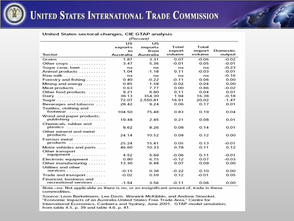
• Interesting to compare ITC assessment to CIE assessment – CIE pushed edges of the analytical envelope.

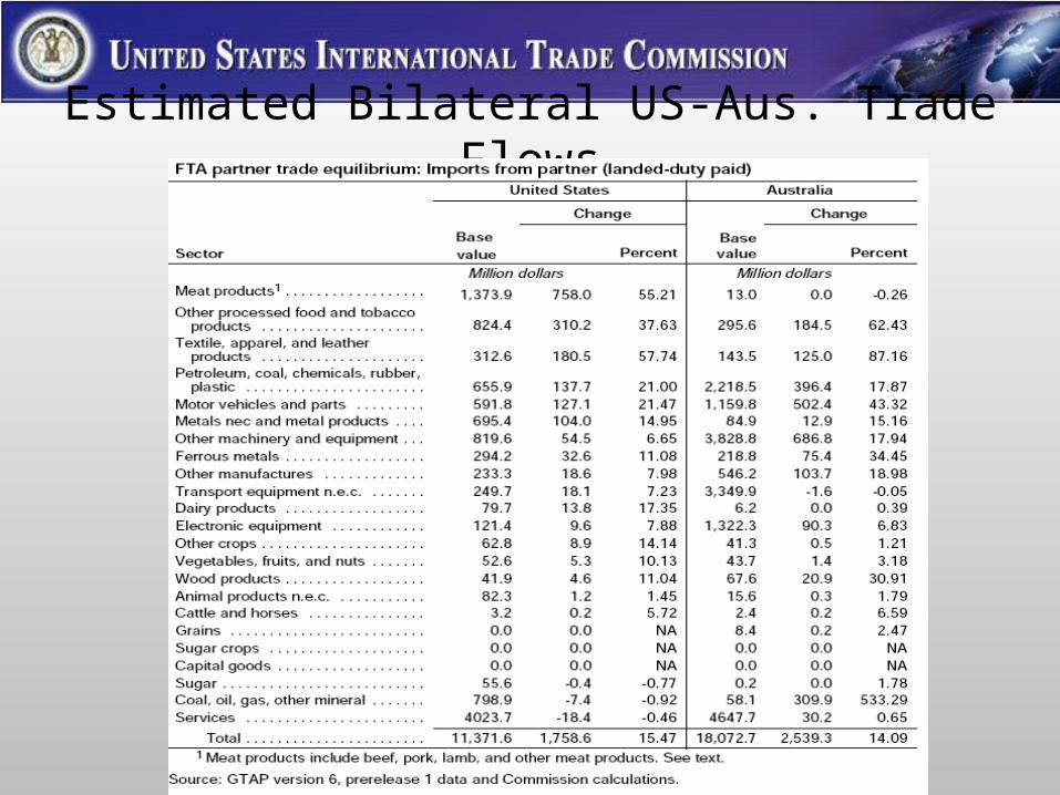
Estimated Bilateral US-Aus. Trade Flows

Estimated US-World Trade Flows

Range of possible “net impacts”

Changes in US output and employment distribution.

Another CGE example: Steel Safeguards

• Often industry seeking protection doesn’t want economy wide effects of protection known.

• Congress has often written safeguard laws to focus on “injured” industry and not the overall effects.

• However not all in Congress agree – example of steel safeguards – Committee wanted to know economy wide effects of safeguards – after they were introduced.

• So what were the benefits to the steel industry and closely related industries of the safeguards, and what were the likely costs to steel users?

• Use economic welfare or income effects.

The political economy dimension?• Economic welfare is really the tip of the iceberg

and often not relevant in economic policy debates– The welfare triangles, which measure the possible net

gains to society, are small compared to the income or revenue rectangles, which capture the income flows diverted by the distortionary policy…

• When looking at the political economy one needs to look at who’s giving up how much, and who’s gaining how much.

The U.S. Steel Safeguard Tariffs Example

Estimated welfare impact – the “small” net number • Central case (Es = 10) -$41.6 million

• Underlying est. income changes – in mil. – the large underlying redistributions– Tariff revenue $649.9– Labor income -386.0– Capital income -294.3

• Iron and steel ind. 239.5• Other pos. affected ind. 67.4• Indus where K income declines -601.2

– Net GDP - 30.4

Another way to think about it is…– All the political action surrounded how the pie was carved up – not by how

much bigger the pie might have been.

Importance of active, independent research agendas for staff…

• Must keep research skills up to date• Contribute to academic and international

research community• Recognition as leading researchers• 2 examples that resulted in APEC, OECD,

and World Bank contributions• Staff research, not Commission findings.

Major research efforts – NTMs/Trade Costs • What are the potential gains from NTMs and trade facilitation?• What are the potential tools for finding out about the gains?

How well do they work?– Inventories of policies and practices– Simple numerical measures– Statistical and econometric tools– Simulation methods– Surveys

• For what purposes might policymakers use quantification?• What are some possible next steps for learning more?

Some estimates of potential gains• Andriamananjara et al. (2004) –

– Global welfare gains from eliminating certain NTMs approximately $90 billion

• Walkenhorst and Yasui (2005) – – Lowering trade transactions costs by 1 percent would improve

global welfare by $40 billion• Wilson, Mann, and Otsuki (2005) –

– Consider improvements in ports, customs, regulation, and service sector infrastructure in countries with below-average performance (halfway to global median)

– Global merchandise trade would increase by $377 billion (9.7 percent)

How much of the markup is due to NTMs?• A “global” estimate (Anderson and Van Wincoop (2004)

– The “typical” cost increase from exporting factory to importing retailer might be 170%

– Markups: 21% transportation, 44% border related trade barriers, 55% retail and wholesale margins

• They can be higher (Tempest (1996))– Barbie dolls cost USD 1 ex-factory in China, USD 2

leaving Hong Kong, and retail for USD 10 in the United States

– Total markup – 900% (“shipping and handling”)

Stages of import port logistics

Source – Londoño-Kent and Kent (2003)

Summary• The USITC is an independent US government agency

that provides the President and Congress with objective analysis.

• The USITC uses many quantitative tools, including CGE, PE, and econometric models (among other techniques) to assess the potential economic impact of trade policy changes.

• USITC studies always combine quantitative and qualitative approaches. ITC economists work closely with industry experts, tariff experts and lawyers to provide a comprehensive perspective.

• Often the abstractions from real world detail required to build economic models limit their stand alone effectiveness to policy makers. However policy makers are frequently looking for “a number” to summarize the benefits and costs of a policy change, and that makes economic models attractive in many cases.