Utah Chapter EERI Short Course, April 9th 2014

Maverik Center, West Valley, Utah

Evaluation and Mitigation

of Liquefaction Hazard

for Engineering Practice

W.D. Liam Finn

Professor Emeritus

University of British Columbia

Show Canterbury Video

Estimates of Residual Shear Strength from SPT-

N Data

Idriss and Boulanger, 2008

Estimates of Residual Strength

Idriss and Boulanger, 2008

Feb. 23rd, 2014

Show Pile Videos

Key Elements in Liquefaction Studies

After Seed et al. 2001

Demand vs Resistance Capacity

For Sands

Demand – PGA and Seismic Shear Stresses

Simplified Method and or Site Response Analysis

Resistance Capacity - - in situ tests – SPT, CPT, Vs

Extreme Measures -Test samples cored from frozen ground

Cyclic Shear Stress Ratio

The Simplified Approach estimates average cyclic

shear stress ratios (CSR) caused by earthquake

shaking using:

Alternative approach is to do site response analyses.

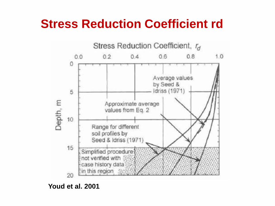
Stress Reduction Coefficient rd

Youd et al. 2001

Magnitude Dependent Stress Reduction Coefficient

Idriss and Boulanger, 2008

Liquefaction resistance curves for M=7.5 by Youd

and Idriss& Boulanger procedures

Note that the differences in rd makes little difference in results.

Correlation with data takes care of it.

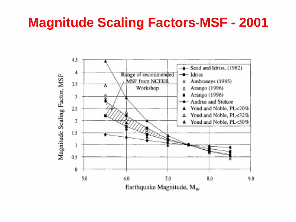
Magnitude Scaling Factors-MSF - 2001

MSF from Idriss and Boulanger (2008)

MSF = min of 6.9exp(−Mw

4 ) − 0.058 or 1.8

Comparison of Youd et al. (2001) and Idriss &

Boulanger (2008) Magnitude Scaling Factors

Liquefaction resistance curves for M=6.0 by Youd

and Idriss& Boulanger procedures

Variations of Kα with SPT & CPT Data

Site Response Analysis for

1. Determination of PGA

and

2. Cyclic shear stresses

This is a developing trend. It is very

prevalent in Vancouver.

Is this the best approach? Much better

than the Simplified Method?

Turkey Flat Instrument Layout

Site Response to Outcrop Input Motions

0

2

4

6

8

10

12

14

16

18

20

0 0.5 1 1.5

Period (sec)

PS

V (

in/s

ec

)10_O1

11A_E1S

12A_E9S

13A_E2S

14A_N7S

16A_E7S

16A_N1S

17A_E3S

17A_E8S

18A_E3S

23A_E11S

Red curve is recorded response - other colors are predictions very

bad predictions.

Probability of liquefaction would be seriously over-estimated.

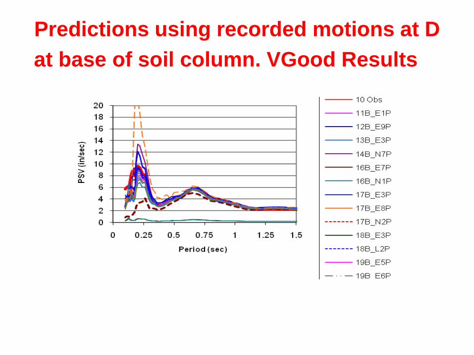
Predictions using recorded motions at D

at base of soil column. VGood Results

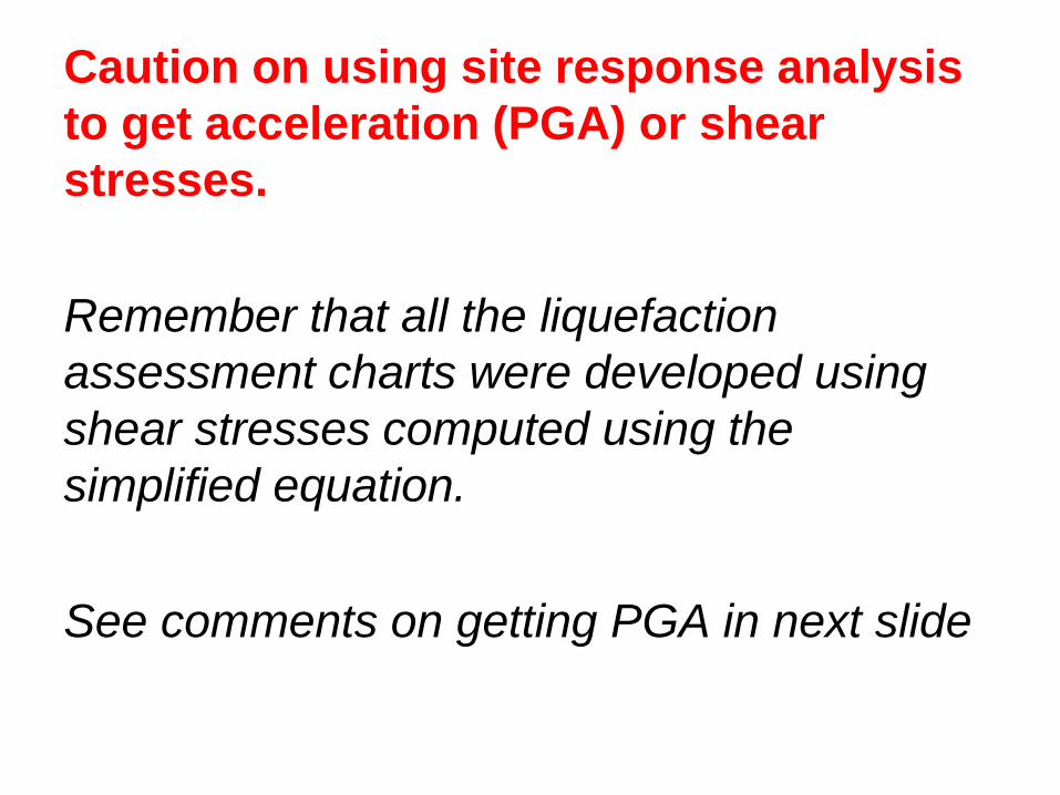
Caution on using site response analysis

to get acceleration (PGA) or shear

stresses.

Remember that all the liquefaction

assessment charts were developed using

shear stresses computed using the

simplified equation.

See comments on getting PGA in next slide

PGA for Simplified Method

“The formal assessment of liquefaction at

a site using the simplified procedure

should be based on the amax that is

estimated to develop in the absence of

soil softening or liquefaction.”

Boulanger and Idriss, 2014

Validation of analytical methods 1

Prediction Exercise 1; Element Tests

Saada and Bianchini (1988) prediction exercise

demonstrated that ability of a model to simulate element

tests is no guarantee of how it will perform in other

element stress fields with different stress paths. Models

need to be calibrated for the dominant stress paths

expected in application as far as is possible with the

conventional tests used in engineering practice.

Feb. 23rd, 2014

Feb. 23rd, 2014

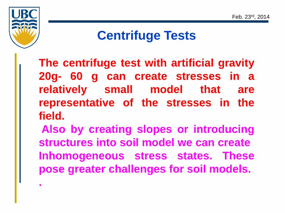
Centrifuge Tests

The centrifuge test with artificial gravity

20g- 60 g can create stresses in a

relatively small model that are

representative of the stresses in the

field.

Also by creating slopes or introducing

structures into soil model we can create

Inhomogeneous stress states. These

pose greater challenges for soil models.

.

Validation of analytical methods 2

Prediction Exercise 2; Centrifuge Tests

Smith (1994) warned about this in his discussion of the

VELACS project which evaluated how well different

constitutive models predicted the results of centrifuge

tests: “A particularly insidious feature of the calibration

process is that a predictor could calibrate his/her model

to fit the bulk of the (largely triaxial) data provided in the

information package and still make poor predictions of

seismically induced stress paths”

Feb. 23rd, 2014

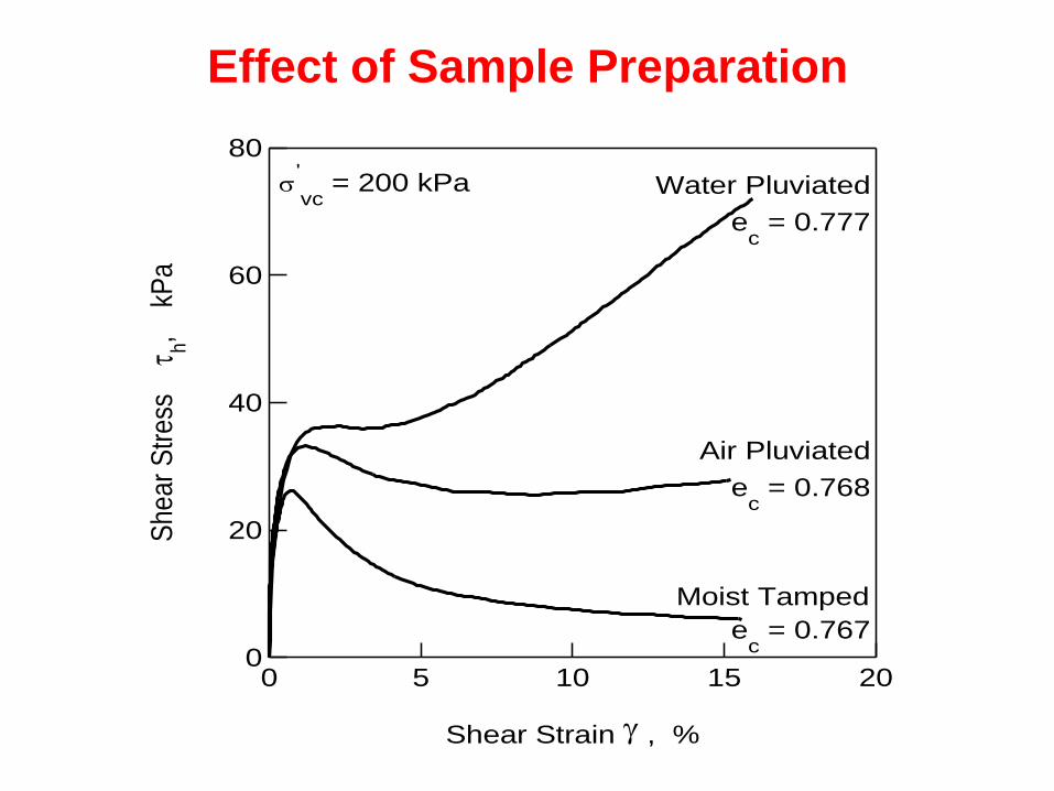
Effect of Sample Preparation

0 5 10 15 20

Shear Strain g , %

0

20

40

60

80S

he

ar

Str

ess

t h,

k

Pa

Water Pluviated

Air Pluviated

Moist Tamped

ec = 0.777

ec = 0.768

ec = 0.767

s'

vc = 200 kPa

Case for Water Pluviation

0 10 20 30

Shear strain g , %

0

50

100

150

200S

hea

r st

ress

t h

, k

Pa s'vc= 114 kPa

e c = 0.893

Frozen

Water Pluviated (KIDD II Sand)

(Massey Sand)

s'vc= 100 kPa

e c = 1.000

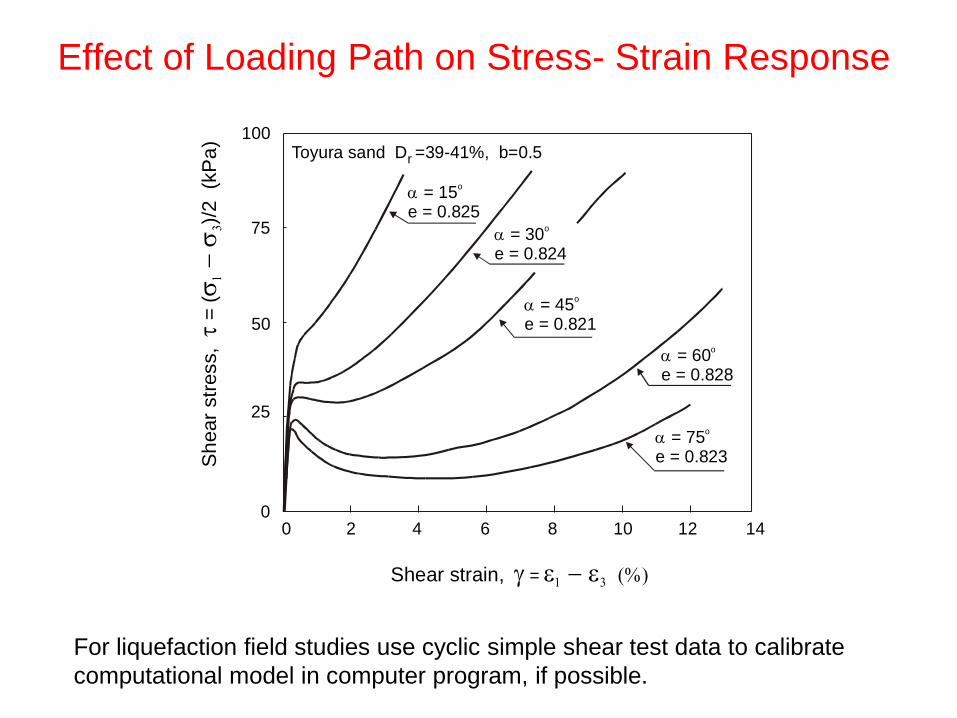
Effect of Loading Path on Stress- Strain Response

Toyura sand D =39-41%, b=0.5r

= 15e = 0.825

o

= 30e = 0.824

o

= 45e = 0.821

o

= 60e = 0.828

o

= 75e = 0.823

o

Shear strain, = g

Sh

ear

str

ess,

= (

)/2

(kP

a)

tss

0

25

50

75

100

0 2 4 6 8 10 12 14

For liquefaction field studies use cyclic simple shear test data to calibrate

computational model in computer program, if possible.

Resistance Capacity

…

Feb. 23rd, 2014

Development of SPT liquefaction triggering

criterion CSR ≥ CRR

Ohsaki 1964 – Whitman1970 – Seed 1976

Seed et al 1985

Youd et al 2001 State of Practice

Idriss and Boulanger,EERI Manual 2008

and associated seminar program leads to

controversy and formation of NSF Committee

to resolve issues by developing an acceptable

new state of practice.

SPT- Liquefaction Assessment Chart

SPT case histories

CPT - Liquefaction Assessment Chart

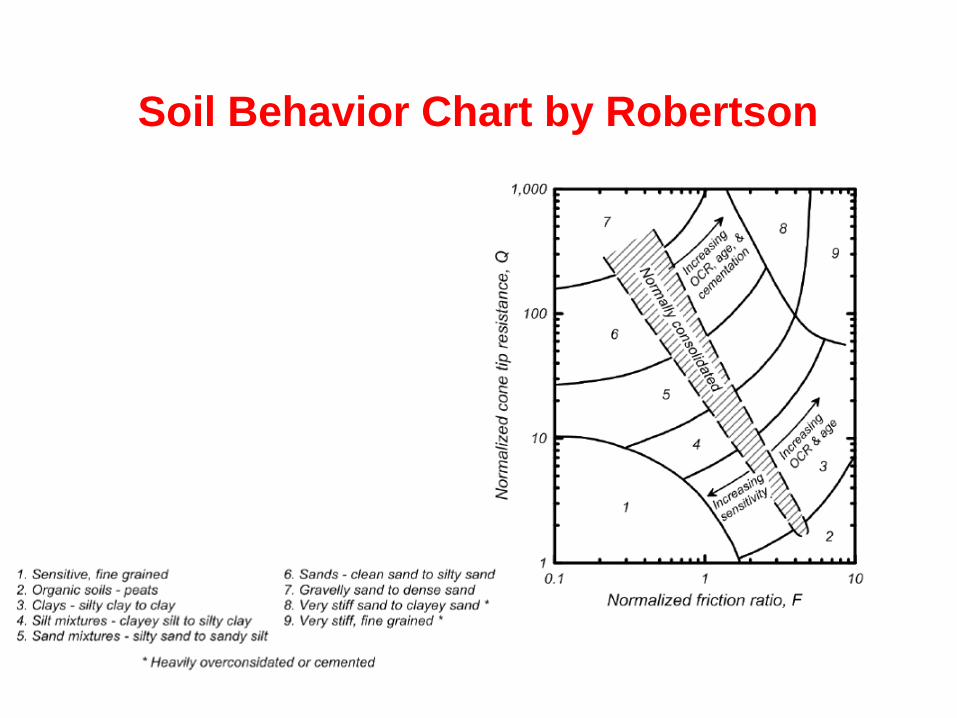
Soil Behavior Chart by Robertson

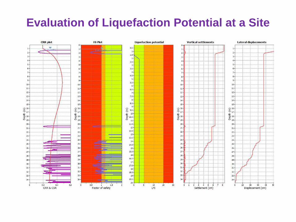
Evaluation of Liquefaction Potential at a Site

Locations of Liquefaction Testing

Contours of Liquefaction Index

Vs-based Liquefaction correlation for clean

uncemented sands (after Andrus & Stokoe 2000)

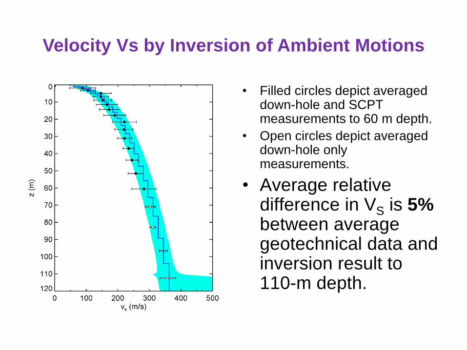
• Filled circles depict averaged down-hole and SCPT measurements to 60 m depth.

• Open circles depict averaged down-hole only measurements.

• Average relative difference in VS is 5% between average geotechnical data and inversion result to 110-m depth.

Velocity Vs by Inversion of Ambient Motions

94-14: LPI = 81

94-15: LPI = 73

94-16: LPI = 63

Downhole: LPI = 77

Liquefaction No Liquefaction

Liquefaction Triggering by Downhole Vs

94-14: LPI = 81

94-15: LPI = 73

94-16: LPI = 63

Downhole: LPI = 77

Inversion: LPI = 69

Liquefaction No Liquefaction

Liquefaction Triggering using Ambient Vs

CRR for Fine Grained Plastic Soils

1.The direct method using cyclic loading tests on

high quality samples.

Otherwise:

2.Measure the monotonic undrained shear

strength, Su, in situ (Vane shear test or from CPT)

or by test on high quality samples or

3.Estimate Su based on the stress history of the soil

profile

Then estimate CRR from Su by empirical

methods

CRRM = 7.5 = (τcyc/Su)N = 30 (Su/σivc)

(13) CRRclay = 0.83 (Su/σi

vc) (14) CRRclay = 0.8 (Su/σi

vc)

(15)

The cyclic shear stress τcyc is 65% of the peak shear stress

as for sand but the ratio

CRRM = 7.5 = (τcyc/Su)N = 30 (Su/σivc)

(τcyc/Su)N = 30 is evaluated from a substantial data base for N = 30 cycles

when M = 7.5.

The value 0.83 was selected for clay-like soils

subjected to direct simple shear loading conditions.

This value may change as more data as more data becomes available.

For the present, CRR is given by

CRRclay = 0.83 (Su/σivc)

If a correction factor C2D = 0.96 is included to represent

the fact that motions occur in the field in two directions then:

CRRclay = 0.8 (Su/σivc)

Evaluating CRR for Fine Grained Plastic Soils

Bjerrum Vane Shear Correction Factor

Magnitude Scaling Factors for Sands and Clays

Boulanger and Idriss 2004

Slope Correction Factor Kα for Plastic Soils

The challenge of probabilistic ground

motions

The simplified method is based on an

associated M and Acceleration

Probabiliistic accelerations result from

contributions of all magnitudes between

considered Mmin and Mmax. So how do you

employ the simplified method?

Serious implications also for lateral spreading

and settlement. Discussed later.

Feb. 23rd, 2014

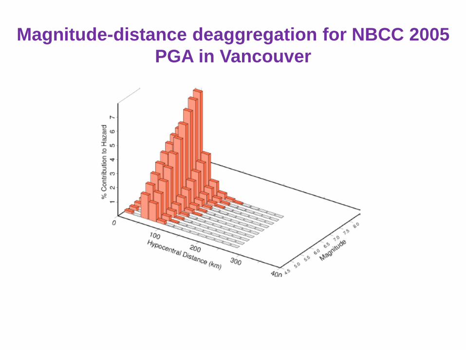
Magnitude-distance deaggregation for NBCC 2005

PGA in Vancouver

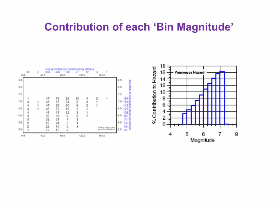
Contribution of each ‘Bin Magnitude’

Liquefaction hazard curve weighted for magnitude M = 7.5

First proposed by Idriss, 1984.

Feb. 23rd, 2014

0 0.2 0.4 0.6 0.8 1PGA (g)

10-5

10-4

10-3

10-2

10-1

Ann

ual F

requ

ency

of E

xcee

danc

e

Vancouver

Seismic Hazard

Liquefaction Hazard

Magnitude-distance deaggregation for NBCC 2005

PGA in Vancouver

Liquefaction potential for various (N1)60,cs values and

seismic site conditions, using Youd et al. (2001)

Maximum cyclic shear strain Vs, FS and Dr

Feb. 23rd, 2014

Expected lateral spreading displacement

Feb. 23rd, 2014

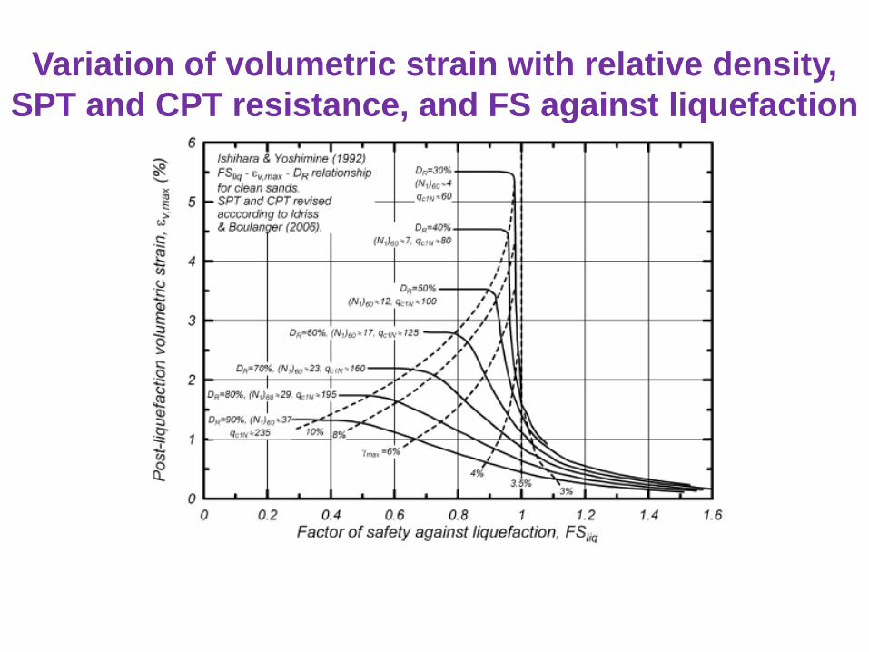
Variation of volumetric strain with relative density,

SPT and CPT resistance, and FS against liquefaction

Overall Vertical Settlements

Measured versus predicted displacements

Lateral Displacement Equation

Youd’s Equation:

Feb. 23rd, 2014

Determining equivalent source distance

The PGA is the average of 3 GMPE for Site Class D

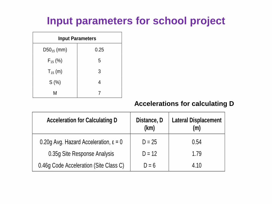
Input parameters for school project

Input Parameters

D5015 (mm) 0.25

F15 (%) 5

T15 (m) 3

S (%) 4

M 7

Acceleration for Calculating D Distance, D (km)

Lateral Displacement (m)

0.20g Avg. Hazard Acceleration, ε = 0

0.35g Site Response Analysis

0.46g Code Acceleration (Site Class C)

D = 25

D = 12

D = 6

0.54

1.79

4.10

Accelerations for calculating D

Sample calculation of lateral spreading

displacements using the deaggregation method

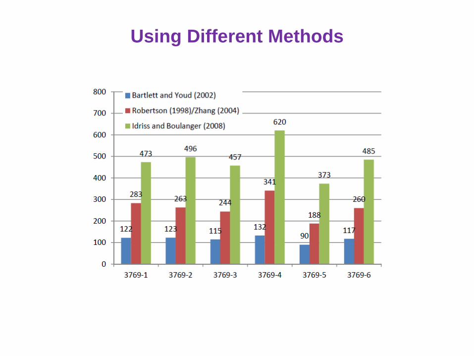
Using Different Methods

Calculated displacements for the school site in Delta

Feb. 23rd, 2014

Closing the Loop

It is the usual procedure in the School Retrofit Program

for the Geotechnical and Structural Engineers get

together with at least two members of the Technical

Review Board to decide how to deal with the

consequences of Liquefaction in the most economical

way.

An example of this cooperation follows for a particular

school. The Structural Engineer involved is John

Sherstobitoff, Ausenco Company, Vancouver, BC. The

slides are abstracted from a recent presentation he made

on the School Project.

Feb. 23rd, 2014

Liquefaction Design Example with Performance Limits

• Building Description

– One storey mixed concrete and steel framed structure

– LDRS Concentric braced frame

(Tension-Compression moderately ductile)

• DDL: 2.5%

– VLS Exterior: Non-ductile concrete columns

• DDL: 1.25%

– VLS Interior/Exterior: Steel columns

• DDL: 4%

– Liquefaction Drift Limit

• LDL: 4% or 2.5% * lesser of the two

• * if liquefaction effects can cause such deformation

concrete

column perimeter grade beams

Pile cap

owsj and metal deck

2500 to 3000 4000 to 7000

3000 steel column steel column

liquefiable layer

S.O.G

tie beam

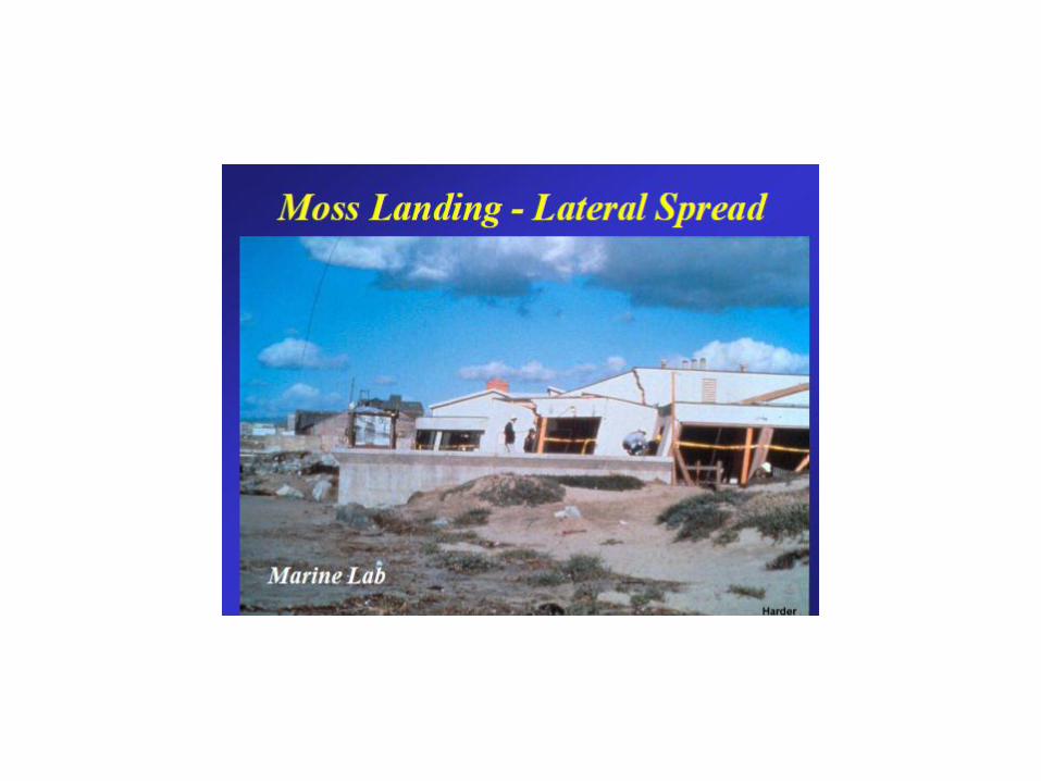
Effects of Lateral Spreading

School building on liquefied soil. Foundations not tied together.

What relative displacement to assign to crack?

Loads from Lateral Spreading on Retrofitted

Foundation

Investigate critical bay for crack location

Liquefaction Drift Limit (LDL)

• Drift Components due to liquefaction – Residual drift (RD)

– Effective drift demand due to lateral soil spreading (EDH)

– Effective drift demand due to vertical soil settlement (EDV)

• RD + EDH + EDV < LDL

L

∆V

∆V

LDRS

not govern

LDRS

can govern

Example from Christchurch

Geotechnical Engineer Input

• Geotechnical Engineer to provide:

– Differential free field vertical movement:

– Differential free field horizontal movement:

– Friction coefficient between soil and foundations:

– Bearing capacity on crust:

– Passive pressure on grade beams:

140 mm

0.4

50 Kpa

600 mm

10xH (m) : P (Kpa)

Differential movement is too large, since the existing foundations are not

adequately tied together in two directions

Based on vertical loads at each foundation provided by the Structural Engineer,

the Geotechnical Engineer will determine if there is risk of punching for each

foundation

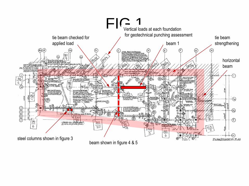
FIG 1

steel columns shown in figure 3 beam shown in figure 4 & 5

beam 1

tie beam checked for

applied load

Vertical loads at each foundation

for geotechnical punching assessment

horizontal

beam

tie beam

strengthening

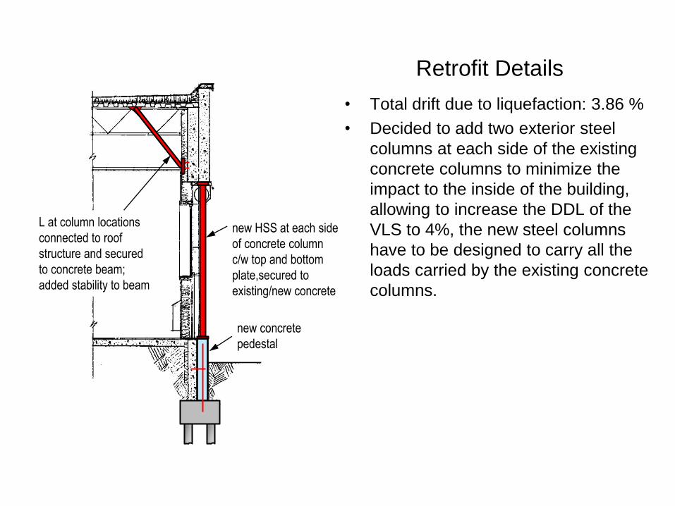
Retrofit Details

• Total drift due to liquefaction: 3.86 %

• Decided to add two exterior steel

columns at each side of the existing

concrete columns to minimize the

impact to the inside of the building,

allowing to increase the DDL of the

VLS to 4%, the new steel columns

have to be designed to carry all the

loads carried by the existing concrete

columns.

new HSS at each side

of concrete column

c/w top and bottom

plate,secured to

existing/new concrete

new concrete

pedestal

L at column locations

connected to roof

structure and secured

to concrete beam;

added stability to beam

new steel

column

concrete

column perimeter grade beam

pile cap

owsj and metal deck

135 mm soil

settlement

steel column steel column

S.O.G

tie beam

Stability of Japanese dykes

• Analyses of dyke failures during Kushiro

Earthquake.

• Soil Properties, input motions and failure

data provided by Japanese.

• Analyses conducted in Vancouver at UBC.

• No interactions during the analyses.

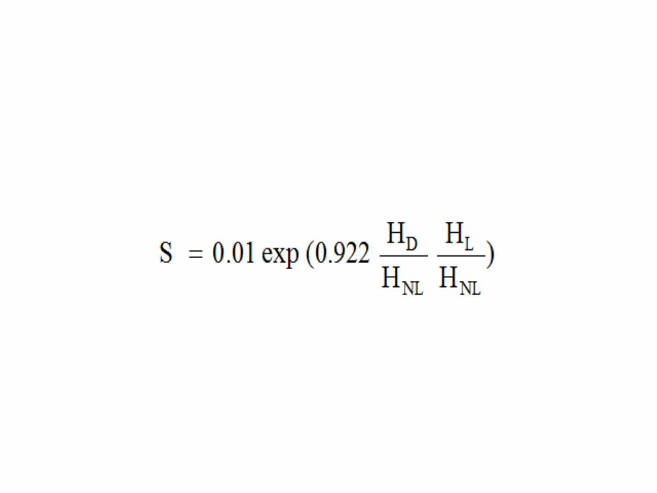
HD

HL

HNL

Sr / s’vo = 0.1 Liquefiable Zone

Non-liquefiable Zone

1:2.5

Typical cross-section of Kushiro dike used in parametric studies

Comparison of observed settlements with the black prediction curve

Eastern Hokkaido Dykes

Western Hokkaido dykes

Subsequent to the Kushiro quake, an earthquake occurred off western Japan, which damaged many Western Dykes. I was invited to Sapporo to discuss the failures and how to prioritize remediation measures.

At the meeting the Japanese presented the results of applying my S-equation to the new set of failures. Fortunately the equation worked extremely well as shown in the next slide.

Comparison of observed settlements for all slopes against

computed settlements for 1:2.5 slopes (solid curve).

Points not close to the curve are for slopes other than 1:2.5

Western Hokkaido Dykes

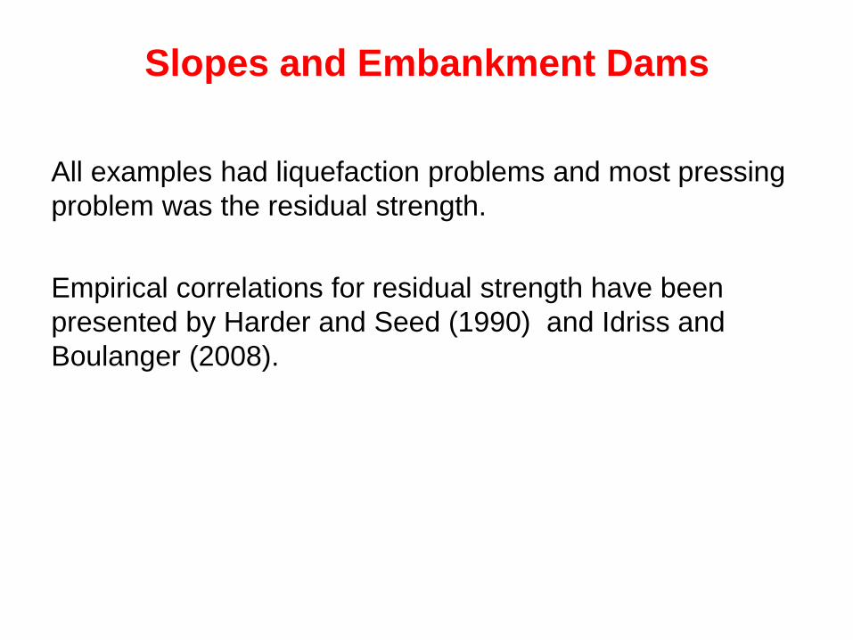
Slopes and Embankment Dams

All examples had liquefaction problems and most pressing

problem was the residual strength.

Empirical correlations for residual strength have been

presented by Harder and Seed (1990) and Idriss and

Boulanger (2008).

Sardis Dam Mississippi, 1988- 1994

This is the first instance of performance

based design of an embankment dam

Cross-section of Sardis Dam

First Example of Performance Based Design

for prioritizing remediation

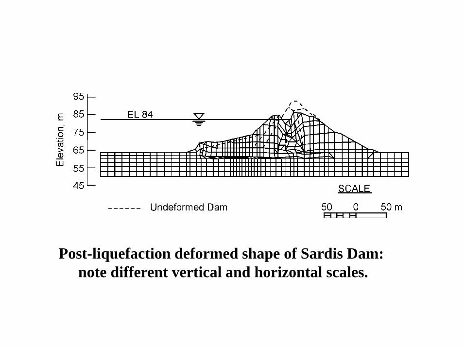
Post-liquefaction deformed shape of Sardis Dam:

note different vertical and horizontal scales.

Factors of safety of Sardis dam as a function

of residual strength in weak foundation layer

Variation of loss of freeboard with

factor of safety of undeformed dam.

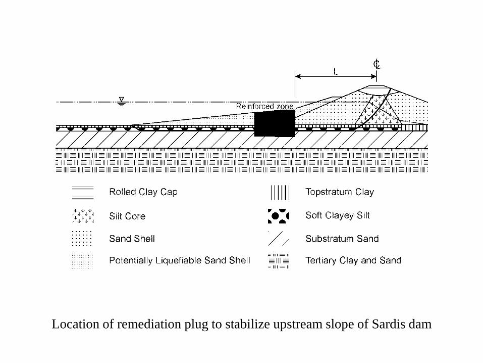
Location of remediation plug to stabilize upstream slope of Sardis dam

Elevation of pile remediation of Sardis dam (after Stacy et al., 1994)

Plan view of pile remediation of Sardis dam (after Stacy et al., 1994)

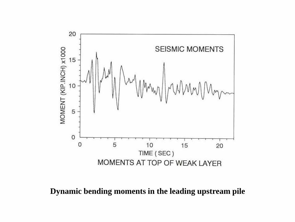
Dynamic bending moments in the leading upstream pile

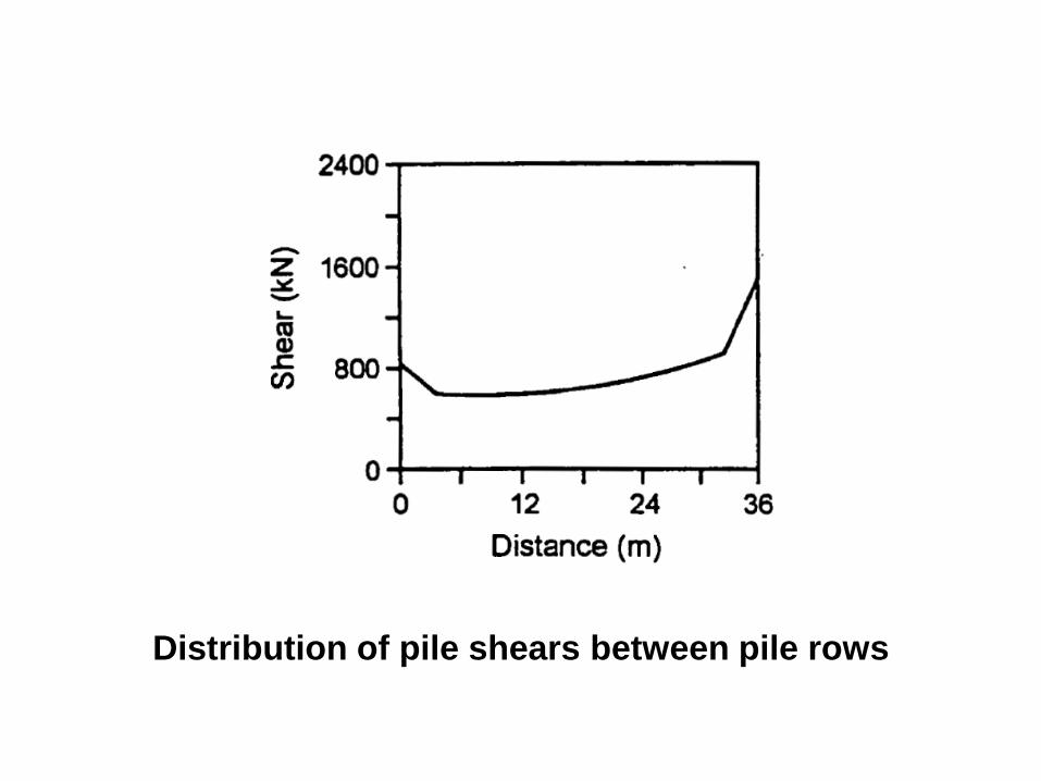
Distribution of pile shears between pile rows

Aerial View of Clemson Diversion Dams (Wooten et al, 2008)

Simplified cross-section Clemson Dams

Cross Section of Remediated Downstream Slope (Wooten et al 2008)

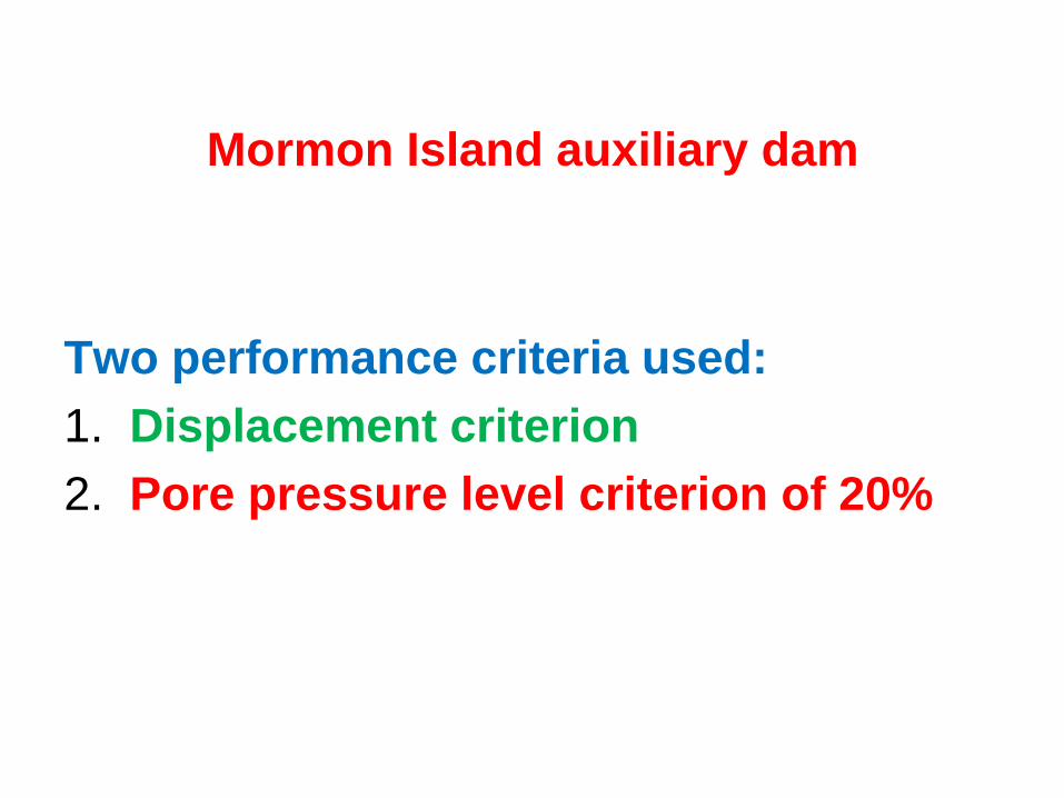
Mormon Island auxiliary dam

Two performance criteria used:

1. Displacement criterion

2. Pore pressure level criterion of 20%