utilizing symmetry in evolutionary design

Utilizing Symmetry in Evolutionary Design

Vinod K. Valsalam

Technical Report AI-10-04

[email protected]://nn.cs.utexas.edu/

Artificial Intelligence LaboratoryThe University of Texas at Austin

Austin, TX 78712

Copyright

by

Vinod K. Valsalam

2010

The Dissertation Committee for Vinod K. Valsalamcertifies that this is the approved version of the following dissertation:


Committee:

Risto Miikkulainen, Supervisor

Dana Ballard

Matthew Campbell

Benjamin Kuipers

Peter Stone


by

Vinod K. Valsalam, B.Tech., M.S.

Dissertation

Presented to the Faculty of the Graduate School of

The University of Texas at Austin

in Partial Fulfillment

of the Requirements

for the Degree of

Doctor of Philosophy

The University of Texas at Austin

August 2010

Acknowledgments

This dissertation was made possible by the excellent support and guidance of my advisor, Risto

Miikkulainen. He has been a constant source of ideas and inspiration for pursuing exciting research.

Working with him has been an invaluable educational experience.

I would not have started my doctoral studies without the encouragement of Robert van de

Geijn. He has continued as a wonderful mentor, providing support and inspiration.

I am very grateful to my committee members, Dana Ballard, Matthew Campbell, Benjamin

Kuipers, and Peter Stone for their insightful comments and constructive criticisms.

I wish to express my sincere gratitude to Greg Plaxton for productive discussions on sorting

networks, including his suggestion to utilize the zero-one principle.

I am also very grateful to Hod Lipson for the opportunity to design and build a robot at

his Cornell Computational Synthesis Laboratory. He and his team of researchers provided expert

guidance, making it possible for me to complete the project in two weeks. In particular, I wish

to thank Ricardo Garcia, Jonathan Hiller, Robert MacCurdy, Franz Nigl, and Michael Tolley for

contributing design ideas and for helping me with unfamiliar tools.

I have benefited immensely from group discussions with the members of the UTCS Neural

Networks research group. Their helpful comments shaped my research and their valuable feedback

improved my presentations.

Finally, I am most grateful to my family for their love, patience, and support while I took

my time to finish the dissertation.

v

This research was supported in part by the National Science Foundation under grants IIS-

0915038, IIS-0757479, and EIA-0303609; the Texas Higher Education Coordinating Board under

grant 003658-0036-2007; Google, Inc.; and the College of Natural Sciences.

VINOD K. VALSALAM

The University of Texas at AustinAugust 2010

vi


Publication No.

Vinod K. Valsalam, Ph.D.

The University of Texas at Austin, 2010

Supervisor: Risto Miikkulainen

Can symmetry be utilized as a design principle to constrain evolutionary search, making

it more effective? This dissertation aims to show that this is indeed the case, in two ways. First,

an approach called ENSO is developed to evolve modular neural network controllers for simulated

multilegged robots. Inspired by how symmetric organisms have evolved in nature, ENSO utilizes

group theory to break symmetry systematically, constraining evolution to explore promising regions

of the search space. As a result, it evolves effective controllers even when the appropriate symmetry

constraints are difficult to design by hand. The controllers perform equally well when transferred

from simulation to a physical robot. Second, the same principle is used to evolve minimal-size sort-

ing networks. In this different domain, a different instantiation of the same principle is effective:

building the desired symmetry step-by-step. This approach is more scalable than previous methods

and finds smaller networks, thereby demonstrating that the principle is general. Thus, evolutionary

vii

search that utilizes symmetry constraints is shown to be effective in a range of challenging applica-

tions.

viii

Contents

Acknowledgments v

Abstract vii

Contents ix

List of Tables xii

List of Figures xiii

Chapter 1 Introduction 11.1 Motivation . . . . . . . . . . . . . . . . . . . . . . . . . . . . . . . . . . . . . . . 11.2 Challenge . . . . . . . . . . . . . . . . . . . . . . . . . . . . . . . . . . . . . . . 21.3 Approach . . . . . . . . . . . . . . . . . . . . . . . . . . . . . . . . . . . . . . . 31.4 Outline of the Dissertation . . . . . . . . . . . . . . . . . . . . . . . . . . . . . . 4

Chapter 2 Foundations 52.1 Biological Motivation . . . . . . . . . . . . . . . . . . . . . . . . . . . . . . . . . 52.2 Symmetries and Group Theory . . . . . . . . . . . . . . . . . . . . . . . . . . . . 62.3 Locomotion Controllers . . . . . . . . . . . . . . . . . . . . . . . . . . . . . . . . 82.4 Sorting Networks . . . . . . . . . . . . . . . . . . . . . . . . . . . . . . . . . . . 122.5 Conclusion . . . . . . . . . . . . . . . . . . . . . . . . . . . . . . . . . . . . . . 13

Chapter 3 Related Work 143.1 Indirect Encodings . . . . . . . . . . . . . . . . . . . . . . . . . . . . . . . . . . 143.2 Multilegged Locomotion . . . . . . . . . . . . . . . . . . . . . . . . . . . . . . . 173.3 Sorting Networks . . . . . . . . . . . . . . . . . . . . . . . . . . . . . . . . . . . 193.4 Conclusion . . . . . . . . . . . . . . . . . . . . . . . . . . . . . . . . . . . . . . 22

Chapter 4 Evolving Modular Controllers 234.1 Quadruped Robot Model . . . . . . . . . . . . . . . . . . . . . . . . . . . . . . . 234.2 Hand-Designed Controller . . . . . . . . . . . . . . . . . . . . . . . . . . . . . . 234.3 Non-modular Controller . . . . . . . . . . . . . . . . . . . . . . . . . . . . . . . 24

ix

4.4 Modular Controller . . . . . . . . . . . . . . . . . . . . . . . . . . . . . . . . . . 264.5 Experimental Setup . . . . . . . . . . . . . . . . . . . . . . . . . . . . . . . . . . 264.6 Walking on Flat Ground . . . . . . . . . . . . . . . . . . . . . . . . . . . . . . . 274.7 Negotiating Obstacles . . . . . . . . . . . . . . . . . . . . . . . . . . . . . . . . . 304.8 Scaling to a Hexapod . . . . . . . . . . . . . . . . . . . . . . . . . . . . . . . . . 314.9 Scaling to Universal Joints . . . . . . . . . . . . . . . . . . . . . . . . . . . . . . 324.10 Conclusion . . . . . . . . . . . . . . . . . . . . . . . . . . . . . . . . . . . . . . 34

Chapter 5 Evolving Controller Symmetries 355.1 Symmetry-Breaking Approach (ENSO) . . . . . . . . . . . . . . . . . . . . . . . 35

5.1.1 Symmetry Evolution . . . . . . . . . . . . . . . . . . . . . . . . . . . . . 355.1.2 Module Evolution . . . . . . . . . . . . . . . . . . . . . . . . . . . . . . 37

5.2 Quadruped Controller . . . . . . . . . . . . . . . . . . . . . . . . . . . . . . . . . 385.3 Experimental Methods . . . . . . . . . . . . . . . . . . . . . . . . . . . . . . . . 395.4 Experimental Setup . . . . . . . . . . . . . . . . . . . . . . . . . . . . . . . . . . 405.5 Walking on Flat Ground . . . . . . . . . . . . . . . . . . . . . . . . . . . . . . . 415.6 Walking on Inclined Ground . . . . . . . . . . . . . . . . . . . . . . . . . . . . . 455.7 Generalization to Reduced Friction . . . . . . . . . . . . . . . . . . . . . . . . . . 475.8 Conclusion . . . . . . . . . . . . . . . . . . . . . . . . . . . . . . . . . . . . . . 50

Chapter 6 From Simulation to Reality 516.1 Evolving Controllers for Real Robots . . . . . . . . . . . . . . . . . . . . . . . . 516.2 Parts and Design . . . . . . . . . . . . . . . . . . . . . . . . . . . . . . . . . . . 526.3 Extending the Simulation . . . . . . . . . . . . . . . . . . . . . . . . . . . . . . . 536.4 Control Programs . . . . . . . . . . . . . . . . . . . . . . . . . . . . . . . . . . . 566.5 All Legs Enabled . . . . . . . . . . . . . . . . . . . . . . . . . . . . . . . . . . . 576.6 Generalization to Reduced Motor Speed . . . . . . . . . . . . . . . . . . . . . . . 596.7 Generalization to Different Leg Positions . . . . . . . . . . . . . . . . . . . . . . 616.8 One Leg Disabled . . . . . . . . . . . . . . . . . . . . . . . . . . . . . . . . . . . 616.9 Conclusion . . . . . . . . . . . . . . . . . . . . . . . . . . . . . . . . . . . . . . 63

Chapter 7 Evolving Sorting Networks 667.1 Boolean Function Representation . . . . . . . . . . . . . . . . . . . . . . . . . . . 667.2 Symmetry-Building Approach . . . . . . . . . . . . . . . . . . . . . . . . . . . . 68

7.2.1 Network Symmetries . . . . . . . . . . . . . . . . . . . . . . . . . . . . . 687.2.2 Defining Subgoal Sequence . . . . . . . . . . . . . . . . . . . . . . . . . 697.2.3 Minimizing Comparator Requirement . . . . . . . . . . . . . . . . . . . . 72

7.3 Evolving Minimal-Size Networks . . . . . . . . . . . . . . . . . . . . . . . . . . 747.4 Results . . . . . . . . . . . . . . . . . . . . . . . . . . . . . . . . . . . . . . . . . 757.5 Conclusion . . . . . . . . . . . . . . . . . . . . . . . . . . . . . . . . . . . . . . 77

x

Chapter 8 Discussion and Future Work 788.1 Hand-Designed Symmetries . . . . . . . . . . . . . . . . . . . . . . . . . . . . . 788.2 Symmetry Evolution with ENSO . . . . . . . . . . . . . . . . . . . . . . . . . . . 798.3 Evolving Controllers for a Physical Robot . . . . . . . . . . . . . . . . . . . . . . 808.4 Utilizing Domain Knowledge in ENSO . . . . . . . . . . . . . . . . . . . . . . . 818.5 Other Applications of ENSO . . . . . . . . . . . . . . . . . . . . . . . . . . . . . 838.6 Extending ENSO . . . . . . . . . . . . . . . . . . . . . . . . . . . . . . . . . . . 838.7 Evolving Sorting Networks . . . . . . . . . . . . . . . . . . . . . . . . . . . . . . 848.8 Conclusion . . . . . . . . . . . . . . . . . . . . . . . . . . . . . . . . . . . . . . 86

Chapter 9 Conclusion 879.1 Contributions . . . . . . . . . . . . . . . . . . . . . . . . . . . . . . . . . . . . . 879.2 Conclusion . . . . . . . . . . . . . . . . . . . . . . . . . . . . . . . . . . . . . . 88

Appendix A Evolved Sorting Networks 89

Bibliography 97

Vita 106

xi

List of Tables

2.1 Gaits corresponding to different combinations of phase shifts θg and θh associatedwith two permutation symmetries g and h of the coupled cell system in Figure 2.3. 11

3.1 The least number of comparators m known to date for sorting networks of inputsizes n ≤ 16. . . . . . . . . . . . . . . . . . . . . . . . . . . . . . . . . . . . . . 20

3.2 The least number of comparators m known to date for sorting networks of inputsizes 17 ≤ n ≤ 32. . . . . . . . . . . . . . . . . . . . . . . . . . . . . . . . . . . 21

7.1 Sizes of the smallest networks for different input sizes found by the EDA. . . . . . 76

xii

List of Figures

1.1 Phase relations between legs in the pronk, pace, bound and trot gaits of quadrupeds. 2

2.1 Representing graph symmetries using groups. . . . . . . . . . . . . . . . . . . . . 72.2 Lattice of subgroups of S4. . . . . . . . . . . . . . . . . . . . . . . . . . . . . . . 92.3 Graph corresponding to the coupled cell system in equation (2.1). . . . . . . . . . 102.4 A 4-input sorting network. . . . . . . . . . . . . . . . . . . . . . . . . . . . . . . 12

3.1 The 16-input sorting network found by Green. . . . . . . . . . . . . . . . . . . . . 20

4.1 The quadruped robot model. . . . . . . . . . . . . . . . . . . . . . . . . . . . . . 244.2 Leg angles specified by the hand-designed controller. . . . . . . . . . . . . . . . . 254.3 Genotypes of the non-modular and modular controller networks for the quadruped

robot model. . . . . . . . . . . . . . . . . . . . . . . . . . . . . . . . . . . . . . . 254.4 Performance of hand-designed, modular, and non-modular neuroevolution controllers

on different terrains and robot models. . . . . . . . . . . . . . . . . . . . . . . . . 284.5 Robot negotiating a terrain with obstacles. . . . . . . . . . . . . . . . . . . . . . . 304.6 Gait changes produced by an evolved modular controller on a terrain with obstacles. 314.7 The hexapod robot model. . . . . . . . . . . . . . . . . . . . . . . . . . . . . . . 324.8 Graph of the coupled cell system for the hexapod robot in Figure 4.7. . . . . . . . 33

5.1 Examples of genotype, phenotype, network module, and color mutation. . . . . . . 375.2 Modular controller network for the quadruped robot model. . . . . . . . . . . . . . 395.3 Performance of controllers evolved using ENSO, random symmetry breaking, fixed

S4 symmetry, and fixed D2 symmetry methods on flat and inclined ground. . . . . 425.4 Phenotype graphs of typical champion networks evolved by ENSO and random

symmetry evolution on flat ground. . . . . . . . . . . . . . . . . . . . . . . . . . . 435.5 Example gaits of champion networks evolved by the different methods on flat ground. 445.6 Phenotype graphs of typical champion networks evolved by ENSO and random

symmetry evolution on inclined ground. . . . . . . . . . . . . . . . . . . . . . . . 475.7 Example gaits of champion networks evolved by the different methods on inclined

ground. . . . . . . . . . . . . . . . . . . . . . . . . . . . . . . . . . . . . . . . . 48

6.1 Back and front views of the Dynamixel AX-12+ motor. . . . . . . . . . . . . . . . 53

xiii

6.2 Top and bottom views of the CM-2+ circuit board. . . . . . . . . . . . . . . . . . 546.3 Assembled physical quadruped robot. . . . . . . . . . . . . . . . . . . . . . . . . 556.4 Simulation of the physical quadruped robot. . . . . . . . . . . . . . . . . . . . . . 556.5 Angular position sensor readings of the Dynamixel AX-12+ motor. . . . . . . . . . 566.6 Phenotype graph of a champion neural network controller evolved by ENSO. . . . 576.7 A trot gait evolved in simulation and transferred to the real robot. . . . . . . . . . . 586.8 Trot gait produced by the hand-designed controller for the real robot. . . . . . . . . 596.9 Gaits produced by the hand-designed and evolved controllers on the real robot when

the maximum speed of the motors is reduced. . . . . . . . . . . . . . . . . . . . . 606.10 Gaits produced by the hand-designed and evolved controllers on the real robot when

the left-rear leg is initialized with maximum angular position error. . . . . . . . . . 626.11 Phenotype graph of a champion neural network controller evolved with the left-rear

leg disabled. . . . . . . . . . . . . . . . . . . . . . . . . . . . . . . . . . . . . . . 636.12 A gait evolved in simulation with the left-rear leg disabled and transferred to the

similarly disabled real robot. . . . . . . . . . . . . . . . . . . . . . . . . . . . . . 64

7.1 Boolean output functions of a 4-input sorting network. . . . . . . . . . . . . . . . 677.2 Representation of monotone Boolean functions on four variables in the Boolean

lattice. . . . . . . . . . . . . . . . . . . . . . . . . . . . . . . . . . . . . . . . . . 687.3 Symmetries of output function duals in 4-input sorting networks. . . . . . . . . . . 707.4 Subgoals for constructing a 4-input sorting network with minimum number of com-

parators. . . . . . . . . . . . . . . . . . . . . . . . . . . . . . . . . . . . . . . . . 717.5 Comparator sharing to compute dual output functions in a 4-input sorting network. 737.6 State representation of the function x1 ∧ x2 utilized in the EDA. . . . . . . . . . . 75

8.1 A two-level hierarchical genotype and phenotype. . . . . . . . . . . . . . . . . . . 82

A.1 Evolved 9-input network with 25 comparators. . . . . . . . . . . . . . . . . . . . . 89A.2 Evolved 10-input network with 29 comparators. . . . . . . . . . . . . . . . . . . . 90A.3 Evolved 11-input network with 35 comparators. . . . . . . . . . . . . . . . . . . . 90A.4 Evolved 12-input network with 39 comparators. . . . . . . . . . . . . . . . . . . . 90A.5 Evolved 13-input network with 45 comparators. . . . . . . . . . . . . . . . . . . . 90A.6 Evolved 14-input network with 51 comparators. . . . . . . . . . . . . . . . . . . . 91A.7 Evolved 15-input network with 57 comparators. . . . . . . . . . . . . . . . . . . . 91A.8 Evolved 16-input network with 60 comparators. . . . . . . . . . . . . . . . . . . . 91A.9 Evolved 17-input network with 71 comparators. . . . . . . . . . . . . . . . . . . . 92A.10 Evolved 18-input network with 78 comparators. . . . . . . . . . . . . . . . . . . . 92A.11 Evolved 19-input network with 86 comparators. . . . . . . . . . . . . . . . . . . . 93A.12 Evolved 20-input network with 92 comparators. . . . . . . . . . . . . . . . . . . . 93A.13 Evolved 21-input network with 103 comparators. . . . . . . . . . . . . . . . . . . 94A.14 Evolved 22-input network with 108 comparators. . . . . . . . . . . . . . . . . . . 94A.15 Evolved 23-input network with 118 comparators. . . . . . . . . . . . . . . . . . . 95A.16 Evolved 24-input network with 125 comparators. . . . . . . . . . . . . . . . . . . 96

xiv

Chapter 1

Introduction

Imagine having to design a multilegged robot to explore Mars. Such a robot could navigate therugged terrains of Mars better than a wheeled robot, but designing a controller for it is more chal-lenging. The controller must coordinate its legs properly, generating robust gaits to navigate dif-ferent terrains effectively while maintaining its stability. Moreover, the robot should be robust todifferent environmental conditions, wear and tear, and even failure like losing one or more legs, toreliably complete its mission.

Designing such controllers is an excellent example of the challenges faced in designingcomplex distributed systems in general. Hand-design is generally difficult and brittle because it ishard to anticipate all operating conditions. Therefore, automatic design utilizing learning techniquessuch as evolution would be desirable. However, the large design space of such systems often makesevolutionary search ineffective. This dissertation focuses on utilizing symmetry to constrain thesearch space in a way that makes evolutionary design possible in a range of interesting complexsystems.

1.1 Motivation

Distributed control systems can be modeled as interconnected components called modules. Forexample, the controller for a multilegged robot can be implemented as a system of interconnectedneural network modules, each controlling a different leg (Beer et al., 1989). Some of these modulesand interconnections may be identical, resulting in symmetries, i.e. permutations of modules thatleave the solution invariant. Symmetries express constraints crucial for designing effective systems;for instance they determine the type of gaits that a multilegged robot controller can produce (Collinsand Stewart, 1993).

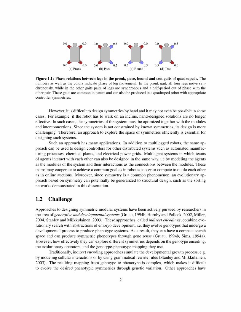
In some cases, it is possible to design the appropriate symmetries by hand. For example,the controller symmetries required to produce the common quadruped gaits seen in nature, suchas pronk, pace, bound, and trot (Figure 1.1) can be designed analytically (Collins and Stewart,1993). These symmetries specify which controller modules and interconnections are identical, thussimplifying the design problem to optimizing only the set of modules and interconnections that areactually distinct.

1

0.0

0.0 0.0

0.0

(a) Pronk

0.0

0.0 0.5

0.5

(b) Pace

0.0

0.5 0.5

0.0

(c) Bound

0.0

0.5 0.0

0.5

(d) Trot

Figure 1.1: Phase relations between legs in the pronk, pace, bound and trot gaits of quadrupeds. Thenumbers as well as the colors indicate phase of leg movement. In the pronk gait, all four legs move syn-chronously, while in the other gaits pairs of legs are synchronous and a half-period out of phase with theother pair. These gaits are common in nature and can also be produced in a quadruped robot with appropriatecontroller symmetries.

However, it is difficult to design symmetries by hand and it may not even be possible in somecases. For example, if the robot has to walk on an incline, hand-designed solutions are no longereffective. In such cases, the symmetries of the system must be optimized together with the modulesand interconnections. Since the system is not constrained by known symmetries, its design is morechallenging. Therefore, an approach to explore the space of symmetries efficiently is essential fordesigning such systems.

Such an approach has many applications. In addition to multilegged robots, the same ap-proach can be used to design controllers for other distributed systems such as automated manufac-turing processes, chemical plants, and electrical power grids. Multiagent systems in which teamsof agents interact with each other can also be designed in the same way, i.e by modeling the agentsas the modules of the system and their interactions as the connections between the modules. Theseteams may cooperate to achieve a common goal as in robotic soccer or compete to outdo each otheras in online auctions. Moreover, since symmetry is a common phenomenon, an evolutionary ap-proach based on symmetry can potentially be generalized to structural design, such as the sortingnetworks demonstrated in this dissertation.

1.2 Challenge

Approaches to designing symmetric modular systems have been actively pursued by researchers inthe area of generative and developmental systems (Gruau, 1994b, Hornby and Pollack, 2002, Miller,2004, Stanley and Miikkulainen, 2003). These approaches, called indirect encodings, combine evo-lutionary search with abstractions of embryo development, i.e. they evolve genotypes that undergo adevelopmental process to produce phenotype systems. As a result, they can have a compact searchspace and can produce symmetric phenotypes through gene reuse (Gruau, 1994b, Sims, 1994a).However, how effectively they can explore different symmetries depends on the genotype encoding,the evolutionary operators, and the genotype-phenotype mapping they use.

Traditionally, indirect encoding approaches simulate the developmental growth process, e.g.by modeling cellular interactions or by using grammatical rewrite rules (Stanley and Miikkulainen,2003). The resulting mapping from genotype to phenotype is complex, which makes it difficultto evolve the desired phenotypic symmetries through genetic variation. Other approaches have

2

been developed that abstract the developmental process. For example, HyperNEAT uses functioncomposition to capture the essential characteristics of this process without implementing it explicitly(Stanley, 2007, Stanley et al., 2009). As a result, phenotypic symmetries can be encoded directlyinto the genotype as symmetric functions. However, composing a manually specified set of primitivefunctions may not be an effective way to explore the space of useful symmetries. For example, itwas necessary to include external oscillations to quadruped controllers evolved with HyperNEAT togenerate gaits, and even such external forcing could not produce the symmetric gaits illustrated inFigure 1.1 (Clune et al., 2009).

These approaches represent symmetry implicitly in the genotype, i.e. they rely on develop-mental processes and function compositions to produce symmetries in the phenotype. As a result,evolution cannot search for symmetries directly, making it difficult to optimize them. Addressingthis issue, this dissertation develops an evolutionary approach that makes symmetry search effectiveby representing symmetry explicitly.

1.3 Approach

The main insight of this approach is that symmetry is an organizing principle, making it possibleto define other essential characteristics of development such as reuse and modularity in terms ofsymmetry. This approach, called Evolution of Network Symmetry and mOdularity (ENSO), uti-lizes group theory, the mathematical theory of symmetry, to represent symmetries explicitly as theconstraints between a given number of modules. The resulting genotype is compact, storing the pa-rameters of identical modules only once, while allowing variations between them to evolve. It usesa simple genotype-phenotype mapping that makes the entire space of phenotype properties easilyaccessible to evolutionary search.

Group theory exposes the structure of the space of symmetries, making it possible to searchfor symmetries directly and also to constrain the search to promising regions of the space. ENSOperforms this search by defining genetic variation (mutation) operators that explore the space ofsymmetries systematically. It initializes evolution with a population of maximally symmetric solu-tions: They have the simplest possible structure, consisting of identical modules and interconnec-tions. During evolution, mutations break their symmetries systematically, thus exploring less sym-metric, more complex solutions with different types of modules and interconnections. As a result,evolution can optimize the modules and interconnections for simpler solutions first and elaboratethem to create more complex solutions. Moreover, the systematic, symmetry-breaking mutationsconstrain search to promising symmetries, making evolution more effective than mutating symmetryunsystematically.

These features make it possible for ENSO to solve complex problems such as the designof distributed controllers and multiagent systems. For instance in this dissertation, ENSO evolveseffective neural network controllers for a quadruped robot in physically realistic simulations. Theresulting controllers produce robust gaits such as those in Figure 1.1. Moreover, they performequally well when they are transferred to a physical robot. ENSO also evolves controllers thatproduce effective gaits for a robot on an incline and for a robot with a faulty leg, scenarios in whichthe appropriate symmetries are difficult to design by hand.

3

Thus evolving symmetries through symmetry breaking is effective when solving the prob-lem requires finding the appropriate symmetries. In other problems the symmetries of the solutionmay already be known, and the challenge is to construct from scratch an optimal solution thatpossesses those symmetries. As shown in this dissertation, such problems may be amenable toa symmetry building approach. For example, the problem of designing minimal-size sorting net-works (Knuth, 1998) can be made easier to solve utilizing this generalization. The source codeimplementing these approaches is available from the website http://nn.cs.utexas.edu/?symmetry.

1.4 Outline of the Dissertation

This dissertation is organized into four main parts: background (Chapters 1-3), symmetry breakingwith multilegged robots (Chapters 4-6), symmetry building with sorting networks (Chapter 7), anddiscussion (Chapters 8-9).

Chapter 2 discusses the biological motivation for the symmetry-breaking principle of ENSO,reviews the fundamental concepts of group theory, and applies those concepts to describe the sym-metries of multilegged locomotion and sorting networks.

Chapter 3 is a survey of previous approaches to evolving symmetric and modular systems,designing controllers for multilegged robots, and designing minimal-size sorting networks.

Chapter 4 lays the groundwork for the ENSO approach. It introduces the multilegged robotmodel used in the simulations, its neural network controller architectures, and shows how evolutionconstrained with hand-designed symmetries produces better controllers than unconstrained evolu-tion and hand-coding.

Chapter 5 introduces the ENSO approach and describes its genotype, phenotype, and evo-lutionary mechanisms. ENSO is then utilized to evolve controllers for a quadruped walking on flatground and a more challenging incline. They are compared with controllers evolved with randomsymmetry mutations and hand-designed symmetries and are shown to perform better.

Chapter 6 presents the design, manufacture, and experimental evaluation of a physicalquadruped robot. ENSO is shown to be an effective method for designing controllers for suchrobots.

Chapter 7 extends the symmetry-based approach for constraining search to designing minimal-size sorting networks, improving on several previously known best results.

Chapter 8 discusses the implications of results presented in previous chapters and suggestsways to improve them. Several extensions and potential applications of ENSO and symmetry build-ing are proposed.

Chapter 9 summarizes the contributions and concludes this dissertation.

4

http://nn.cs.utexas.edu/?symmetry

http://nn.cs.utexas.edu/?symmetry

Chapter 2

Foundations

Nature has evolved a variety of symmetric organisms, motivating a symmetry-based approach forthe evolutionary design of artificial systems as well. This chapter begins by discussing this moti-vation and then reviews the group theory concepts required for utilizing symmetry in evolutionaryalgorithms. To make the approach concrete, these concepts are applied to represent the symmetriesof controllers for multilegged robots and those of sorting networks. Representing symmetries in thismanner makes it possible to constrain the design space to promising solutions. As a result, largeand challenging design problems becomes more tractable, as demonstrated in later chapters.

2.1 Biological Motivation

Symmetry is the product of constraints between identical subsystems. For example, a bilaterallysymmetric animal has identical left and right legs that are constrained to be equidistant from its planeof symmetry, and the symmetric neural circuitry controlling its locomotion has identical modulesconstrained by the nature of their interconnections (Collins and Stewart, 1993). Symmetry in suchsystems provides two benefits: (1) it can make evolutionary search easier by encoding identicalsubsystems compactly using a common set of genes, and (2) it can produce useful phenomena suchas patterned oscillations in neural circuits, e.g. for effective gaits.

How did organisms with different symmetries evolve in nature? Fossil evidence suggeststhat more symmetric organisms evolved into less symmetric organisms (Martindale and Henry,1998, Palmer, 2004). For example, primitive, single-celled organisms like protozoans are highlysymmetric with spherical shapes. They evolved into less symmetric organisms such as jelly fish,which have radial symmetry. And radially symmetric organisms in turn evolved into even lesssymmetric organisms, e.g. the bilaterally symmetric humans. Simply put, nature evolves symmetrythrough symmetry breaking.

Mutations that break symmetries produce novel phenotypic variations (Palmer, 2004). Forexample, fiddler crabs, whose males are asymmetric with an oversized claw, evolved from a bilat-erally symmetric ancestor. Bilateral symmetry is the default in such organisms, i.e. the same devel-opmental program creates paired, symmetric sides. Breaking this symmetry requires the genome

5

to specify additional information on how one side is different from the other, thus increasing thecomplexity of the genome.

In fact, symmetry is fundamentally related to complexity, allowing complexity to be char-acterized as the lack of symmetry (Heylighen, 1999). Increase in complexity of organisms duringevolution is accompanied by symmetry breaking at different levels of organization (Garcia-Bellido,1996). Moreover, complexification, i.e. increasing complexity gradually, makes evolutionary searchmore effective because it allows evolution to start with low-dimensional genotypes, which are easyto optimize, and gradually add more dimensions (Stanley and Miikkulainen, 2004). Building com-plex systems by elaborating solutions in this manner is more likely to succeed than evolving solu-tions in the final high-dimensional space directly. Therefore, evolving complex systems from simplesymmetric systems by breaking symmetry step-by-step might be a good way to design them.

This idea for focusing evolutionary search on promising solutions motivates the symmetrybreaking approach of ENSO discussed in Chapter 5. ENSO represents solutions as graphs andutilizes group theory to represent the symmetries of those graphs, as described next.

2.2 Symmetries and Group Theory

ENSO evolves modular solutions to design problems. It represents the modules as the vertices andthe relationships between them as the edges of a complete graph G = (V,E), where V is the vertexset and E = {(u, v) | u, v ∈ V ; u 6= v} is the edge set. Since G cannot have loops, it is possible torepresent a vertex v by the pair (v, v), and thus represent both vertices and edges by the elements ofthe set V × V . In order to represent the symmetries of G, ENSO assigns every element of V × Va color, producing a complete coloring (Bastert, 2001) of the vertices and edges of G. In practice,each color represents a particular combination of parameters associated with a vertex or an edge. Asymmetry ofG is defined as any permutation of its vertices that preserves the color of edges betweenthem.

The symmetries of a graph can be represented mathematically as a group (Beineke et al.,2004, Chan and Godsil, 1997). A group is a set G of elements closed under a binary operation ◦satisfying the following axioms:

Associativity: For all g, h, k ∈ G, (g ◦ h) ◦ k = g ◦ (h ◦ k).

Identity element: There exists an element e ∈ G such that for all g ∈ G, e ◦ g = g ◦ e = g.

Inverse element: For each g ∈ G, there is an element g−1 ∈ G such that g ◦ g−1 = g−1 ◦ g = e.

The operation g ◦ h is usually written more compactly as gh.A subgroupH of a group G, denotedH ≤ G, is a subset of the group elements of G satisfying

the group axioms under the same operation. If the subset is a proper subset of G, then the subgroupis called a proper subgroup of G. A maximal subgroup of G is any proper subgroup S such that noother proper subgroup T contains S strictly. If G represents the symmetries of a graph G, then itsproper subgroupH represents the symmetries of a less symmetric graph H . ENSO uses this fact tocompare graph symmetries.

6

GA GB

1 2

3 4

1 2

3 4

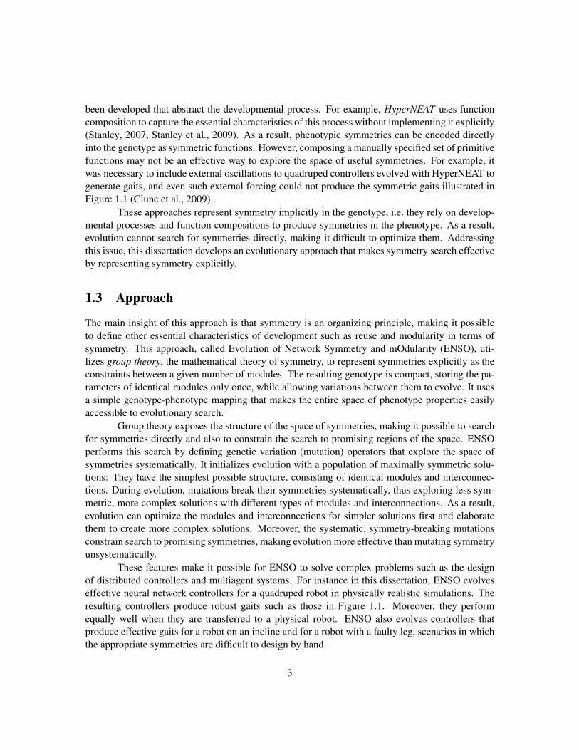
Figure 2.1: Representing graph symmetries using groups. Each vertex and edge has a color (indicatedby both color and line style) representing a particular combination of parameters. A graph symmetry is anypermutation of vertices under which the edge colors remain the same. Both graphs in this figure have verticesof the same color. All edges of graphGA have the same color, while edges of graphGB have different colors.Therefore, any permutation of the vertices of graph GA is a symmetry. In contrast, only the permutationsg = (1 2)(3 4) and h = (1 3)(2 4), and their compositions are symmetries of graph GB . The set of allsymmetries of a graph form a group, with composition as the group operation. Thus group theory is a naturalway to represent symmetries.

Two subgroups S and T are said to be conjugate if there exists an element g ∈ G such thatT = gSg−1, i.e. T = {gsg−1 | s ∈ S}. Conjugacy is an equivalence relation, partitioning the setof all subgroups of a group G into equivalence classes called conjugacy classes. The subgroups be-longing to a given conjugacy class represent graphs with similar symmetries. Therefore, conjugacyclasses are useful for characterizing the space of graph symmetries that ENSO has to search.

Figure 2.1 illustrates how the above definitions can be used to represent the symmetries of acompletely colored graph with four vertices. Since all edges of graph GA have the same color, anypermutation of its vertices is a symmetry of the graph. In contrast, graph GB has fewer symmetriesbecause its edges have different colors. The permutation g = (1 2)(3 4), which swaps vertices 1and 2 as well as vertices 3 and 4, is a symmetry of GB . Similarly, the permutation h = (1 3)(2 4)is another symmetry and their composition hg obtained by performing the two permutations insequence is yet another symmetry. The trivial permutation e = (), which fixes each vertex of thegraph, is also a symmetry. The set of all such symmetries of a graph G is closed under compositionand inverse, i.e. it forms a group with composition as the group operation. This group is called thesymmetry group or automorphism group of G, denoted as Aut(G).

The automorphism group of graph GA, consisting of all 4! permutations of its vertex setV = {1, 2, 3, 4}, is called the symmetric group of degree four, denoted as S4. The automorphismgroup of the less symmetric graph GB is a subgroup of S4 called the dihedral group D2 (andis isomorphic to the symmetries of a regular polygon with two sides, i.e. a line segment). Moregenerally, the automorphism group of any graph G with vertex set V = {1, 2, 3, 4} is a subgroupof S4, and is fully determined by the complete coloring of G. ENSO utilizes this observation tomanipulate the symmetries of graphs by changing their coloring.

Changing the coloring of a graph G such that its new automorphism group is a subgroupof its original automorphism group is said to break the symmetry of G. In order to implementsymmetry breaking, ENSO defines a canonical complete coloring of G for any given automorphism

7

group G using the concept of group action. Formally, the action of G on the vertex set V is a functionG × V → V , denoted (g, v) 7→ g · v for each g ∈ G and each v ∈ V , which satisfies the followingtwo conditions:

1. e · v = v for every v ∈ V , where e is the identity element of G, and

2. (gh) · v = g · (h · v) for all g, h ∈ G and v ∈ V .

The set of allw ∈ V to which v is mapped by the elements of G is called the orbit of v. Similarly, thecoordinate-wise action of G on V ×V is defined as g · (v, w) = (g ·v, g ·w) for any (v, w) ∈ V ×V .The orbits in this action are called orbitals, and they form a partition of V × V called an orbitalpartition. Assigning a different color to each part of this partition produces the desired canonicalcomplete coloring of G.

If a graph G′ is produced by breaking the symmetry of G, then the orbital partition ρ′ underthe action of Aut(G′) is a refinement of the orbital partition ρ under the action of Aut(G), i.e. eachpart of ρ′ is a subset of a part of ρ. Therefore, the canonical complete coloring ofG′ can be obtainedfrom that of G by assigning new colors to the parts of ρ′ that are a proper subset of a part of ρand retaining the colors of parts of ρ′ that are also parts of ρ. ENSO represents this hierarchicalrelationship between the colors of G and G′ by organizing the new colors of G′ as the children ofcolors of G that they replace. This organization produces a tree of colors when symmetry is brokenrepeatedly during evolution.

Breaking symmetry in the above manner induces a partial ordering of the graphs based onthe subgroup relation between their automorphism groups. More precisely, with subgroup as thepartial order relation, the set of all subgroups of a group form a lattice. Figure 2.2 illustrates thislattice for the subgroups of S4. Nodes of this lattice represent conjugacy classes of subgroups. Agroup Gi is placed above another group Gj and connected by a line if and only if Gj is a maximalsubgroup of Gi. This lattice contains the automorphism groups of all completely colored graphswith vertex set V = {1, 2, 3, 4}. The most symmetric graphs with automorphism group S4 are atthe top of the lattice, while the least symmetric graphs with the trivial automorphism group {e} areat the bottom.

ENSO utilizes this ordering of graphs induced by the subgroup lattice to search the space ofgraph symmetries systematically. The above group theory concepts can also be utilized to explainthe symmetries of the two applications considered in this dissertation: multilegged locomotion andsorting networks. For this purpose, multilegged locomotion is abstracted as coupled cell systems,as described next.

2.3 Locomotion Controllers

A coupled cell system consists of a set of dynamical systems, called cells, and a specification of howthe cells are coupled, i.e. how the state of each cell affects the states of the other cells (Golubitskyand Stewart, 2002). Some or all of the cells and couplings may be identical, resulting in symmetriesthat correspond to permutations of the cells under which the behavior of the system is invariant.Such symmetric, coupled cell systems can exhibit synchronous and phase-related periodic patterns

8

D43 x

Z43 x D23 x

Z23 x Z26 x

{e}

Z34 x

D2

A4 S34 x

S4

Figure 2.2: Lattice of subgroups of S4. This lattice was computed using the GAP (2007) software forcomputational group theory and shows the subgroups of the group S4, which is the symmetric group ofdegree four containing all 4! permutations of the set V = {1, 2, 3, 4}. Each node of the lattice represents anequivalence class of conjugate subgroups. There are four types of nodes. The node labeled 4×S3 representsthe four symmetric groups of degree three obtained by fixing each of the four elements of V and permutingonly the other three elements. The node labeled A4 represents the alternating group of degree four, formedby the permutations of V that can be expressed as the composition of an even number of transpositions.The node labeled Dn represent the dihedral groups, formed by the permutations of V that are isomorphicto the symmetries of a regular polygon with n sides. The node labeled Zn represent the cyclic groups,formed by the permutations of V that are isomorphic to the group of integers under addition modulo n. Theautomorphism groups of all graphs with vertex set V appear in this lattice, inducing a partial order of thecorresponding graphs. Thus, the most symmetric graphs with automorphism group S4 appear at the top andthe least symmetric graphs at the bottom of the lattice, with the trivial automorphism group {e} at the verybottom. This order makes it possible for ENSO to search the space of graph symmetries systematically bytraversing the lattice from top to bottom.

in their state. Collins and Stewart (1993) showed that this patterned behavior can be used to modelanimal locomotion and to explain gait symmetries.

Following their method, the modular controllers in this dissertation are also modeled assymmetric coupled cell systems. The patterned oscillatory behavior produced by these symmetriesis independent of the model parameters, i.e. the details of the internal dynamics of the cells do notmatter. Therefore, analyzing the symmetries of a coupled cell system can give insights into thehigh-level qualitative behavior of the system.

This analysis is illustrated below for a coupled cell system due to Pinto and Golubitsky(2006). While they used this system to understand biped locomotion, it is adapted in this reviewto model quadruped gaits. This system consists of four identical cells, described by the following

9

F( , , , )

1 2

3 4

LeftFront

LeftRear

RightRear

RightFront

Figure 2.3: Graph corresponding to the coupled cell system in equation (2.1). The vertices, numbered1 through 4, represent cells and the edges represent coupling between the cells. The different edge colors(also indicated with different line styles) represent different couplings, corresponding to different argumentpositions in function F as shown in the legend. This graph helps visualize the symmetries of the coupled cellsystem and shows how the cells may be assigned to control the legs of a quadruped robot to produce differentgaits (Figure 1.1). For example, these symmetries can constrain cells 1 and 2 to oscillate synchronously withphase opposite to that of similarly synchronous cells 3 and 4, producing the bound gait.

system of ordinary differential equations (ODEs):x1 = F (x1,x2,x3,x4)x2 = F (x2,x1,x4,x3)x3 = F (x3,x4,x1,x2)x4 = F (x4,x3,x2,x1),

(2.1)

where xi ∈ Rk are the k state variables of cell i, and F : (Rk)4 → Rk encapsulates the internaldynamics of each cell and its coupling with other cells. Thus, this system of ODEs describes howthe state variables of each cell change in time as a function of the cell’s own state and the state ofthe other cells.

This system can be represented by the graph in Figure 2.3, which helps visualize its sym-metries. The vertices of the graph represent cells and the edges represent coupling between thecells. Each edge color represents a different type of coupling, corresponding to a different argumentposition in the function F . This graph is the same as the graph GB of Figure 2.1 in Section 2.2,where its symmetries were analyzed. In particular, its automorphism group is D2, consisting of thesymmetric permutations g = (1 2)(3 4), h = (1 3)(2 4), and their composition hg.

Each symmetry of the graph induces a symmetry of the associated system of ODEs, i.e. atransformation γ such that γx(t) is a solution whenever x(t) is a solution. For example, supposex(t) is a solution to (2.1). Applying the permutation g to (2.1) produces an equivalent system ofODEs for which gx(t) is a solution. Thus, the system of ODEs inherits the symmetry g from thecorresponding graph.

In particular, periodic solutions of the system are interesting because they model gaits. Letx(t) be a T -periodic solution to (2.1) and γ be a symmetry. Then γx(t) is also a solution. Becausesolutions to the same initial conditions are unique, if x(t) and γx(t) are the same trajectory, thentheir phases must be different, i.e. γx(t) = x(t+θ) where θ ∈ [0, T ) for all t. Since applying either

10

Pronk Pace Bound Trot

θg 0 T2 0 T

2

θh 0 0 T2

T2

Table 2.1: Gaits corresponding to different combinations of phase shifts θg and θh associated with twopermutation symmetries g and h of the coupled cell system in Figure 2.3. Thus, this system can havesolutions modeling a variety of common quadruped gaits.

g twice or h twice to a solution is equivalent to applying the identity, 2θ ≡ 0 (mod T ) for bothsymmetries. Therefore, the possible values of phase shift θ is either 0 or T

2 for both symmetries.Such phase shifts impose constraints on the components of the solution x(t) = (x1(t),x2(t),x3(t),x4(t)),

producing specific patterned behavior for the system. For example, the bound gait pattern re-sults from the following constraints. The symmetry g is first applied to x(t) with a phase shiftof θg = 0, resulting in the constraints x2(t) = x1(t) and x4(t) = x3(t). Consequently, the solu-tion has the form x(t) = (x1(t),x1(t),x3(t),x3(t)), implying that cells 1 and 2 are synchronousand cells 3 and 4 are synchronous, but their synchrony is independent, i.e. it does not yet pro-duce an interesting gait. However, applying the symmetry h to this solution with a phase shiftof θh = T

2 results in a further constraint x3(t) = x1(t + T2 ). Now, the solution has the form

x(t) = (x1(t),x1(t),x1(t + T2 ),x1(t + T

2 )), implying that cells 1 and 2 are synchronous, whilecells 3 and 4 are also synchronous with the same periodic trajectory as cells 1 and 2, but half-period out of phase. Assigning these cells to control the legs of a quadruped robot as illustrated inFigure 2.3 produces a bound gait (Figure 1.1c).

Other common quadruped gaits (such as those depicted in Figure 1.1) can be obtained sim-ilarly by selecting different combinations of values for θg and θh as shown in Table 2.1. Althoughthese gaits are possible solutions of the system, whether any particular gait can be obtained in aninstance of the system depends on the details of the cell dynamics and the couplings, i.e. on thefunction F in the ODEs. Chapter 4 shows that this function F can be designed effectively by utiliz-ing modular neuroevolution, i.e. by representing each cell as a neural network module and evolvingits weights. The resulting controllers produced all four gaits listed in Table 2.1.

The above theoretical results make the gait-production capabilities of such modular con-troller networks easy to understand. Consequently, in contrast to other approaches, these controllersare easy to design and scale well to robots with more legs and more complex legs (Chapter 4).Moreover, neuroevolution is an effective alternative to designing coupled cell system ODEs man-ually such as was done, e.g. by Collins and Stewart (1993),Kimura et al. (1999), Seo and Slotine(2007), and Righetti and Ijspeert (2008). In Chapter 5, the ENSO approach extends modular neu-roevolution by also evolving the symmetries of the system. As a result, ENSO can evolve controllersthat produce effective gaits even when such gaits are unknown and manual design of the requiredsymmetries is difficult.

The ENSO approach is useful in problems such as distributed control and multiagent sys-tems for which the appropriate symmetries are unknown. In other design problems, the appropriate

11

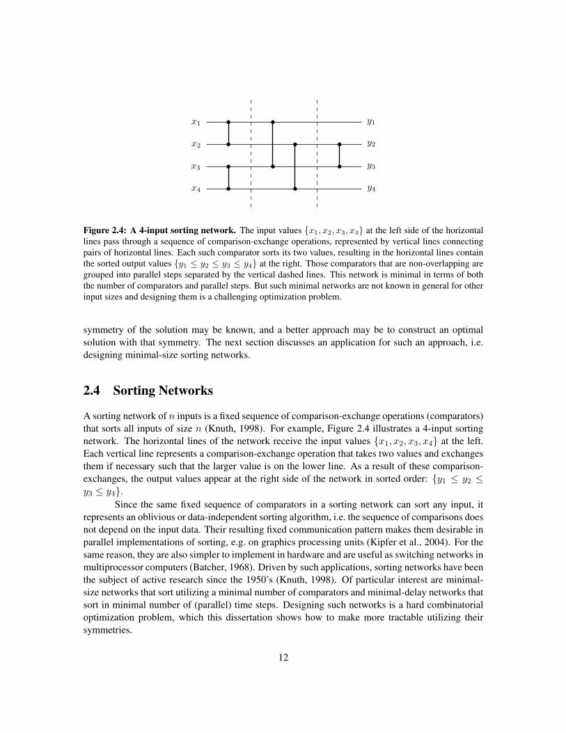
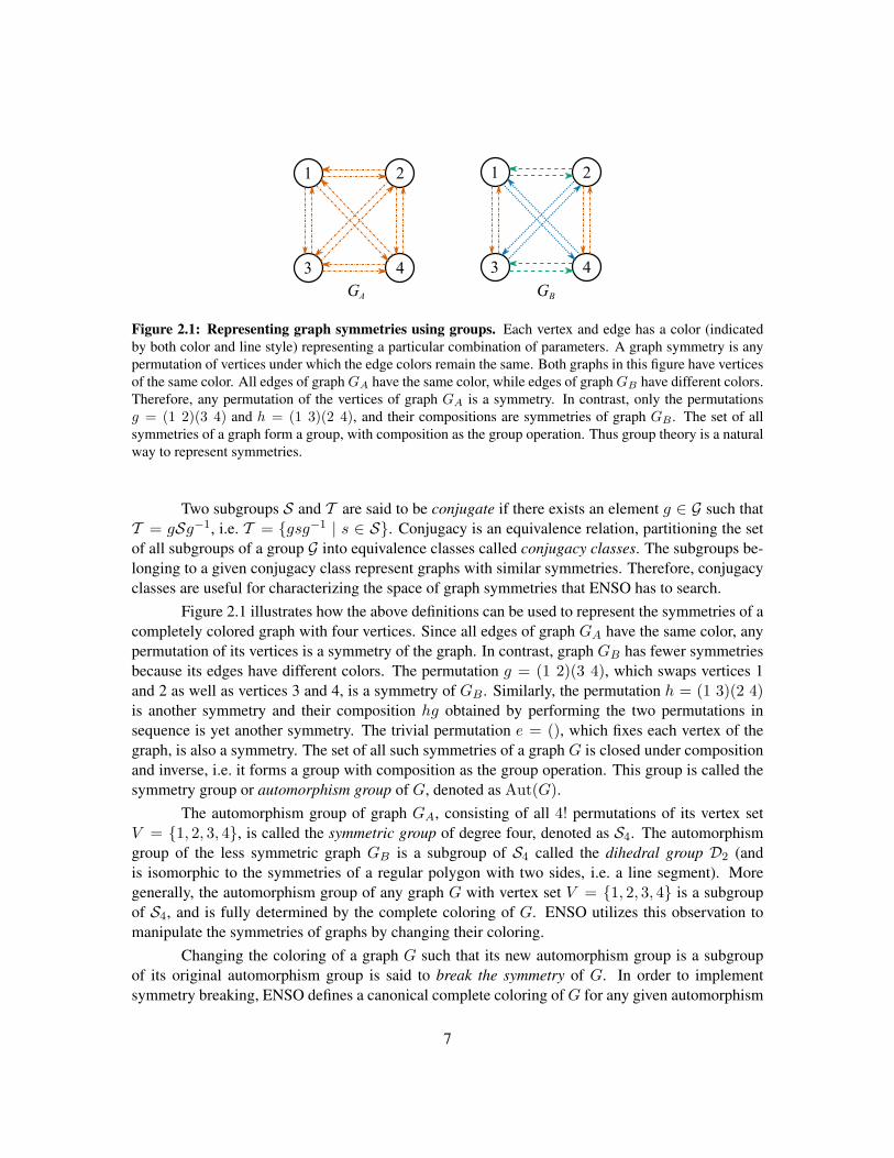
Figure 2.4: A 4-input sorting network. The input values {x1, x2, x3, x4} at the left side of the horizontallines pass through a sequence of comparison-exchange operations, represented by vertical lines connectingpairs of horizontal lines. Each such comparator sorts its two values, resulting in the horizontal lines containthe sorted output values {y1 ≤ y2 ≤ y3 ≤ y4} at the right. Those comparators that are non-overlapping aregrouped into parallel steps separated by the vertical dashed lines. This network is minimal in terms of boththe number of comparators and parallel steps. But such minimal networks are not known in general for otherinput sizes and designing them is a challenging optimization problem.

symmetry of the solution may be known, and a better approach may be to construct an optimalsolution with that symmetry. The next section discusses an application for such an approach, i.e.designing minimal-size sorting networks.

2.4 Sorting Networks

A sorting network of n inputs is a fixed sequence of comparison-exchange operations (comparators)that sorts all inputs of size n (Knuth, 1998). For example, Figure 2.4 illustrates a 4-input sortingnetwork. The horizontal lines of the network receive the input values {x1, x2, x3, x4} at the left.Each vertical line represents a comparison-exchange operation that takes two values and exchangesthem if necessary such that the larger value is on the lower line. As a result of these comparison-exchanges, the output values appear at the right side of the network in sorted order: {y1 ≤ y2 ≤y3 ≤ y4}.

Since the same fixed sequence of comparators in a sorting network can sort any input, itrepresents an oblivious or data-independent sorting algorithm, i.e. the sequence of comparisons doesnot depend on the input data. Their resulting fixed communication pattern makes them desirable inparallel implementations of sorting, e.g. on graphics processing units (Kipfer et al., 2004). For thesame reason, they are also simpler to implement in hardware and are useful as switching networks inmultiprocessor computers (Batcher, 1968). Driven by such applications, sorting networks have beenthe subject of active research since the 1950’s (Knuth, 1998). Of particular interest are minimal-size networks that sort utilizing a minimal number of comparators and minimal-delay networks thatsort in minimal number of (parallel) time steps. Designing such networks is a hard combinatorialoptimization problem, which this dissertation shows how to make more tractable utilizing theirsymmetries.

12

The outputs of any n-input sorting network are invariant to any of the n! permutations of itsinputs because the sorted order at its outputs remains the same. Therefore, it has symmetry groupSn with respect to permutations of its input variables. Moreover, swapping the outputs of everycomparator in the network to move the larger values to their respective upper lines creates a dualnetwork producing outputs in reversed sorted order. This duality can also be expressed formallyas symmetries by utilizing the zero-one principle (Knuth, 1998) to represent the network outputsas Boolean functions. According to this principle, if the network sorts all 2n binary sequencescorrectly, then it will also sort any arbitrary sequence of n numbers correctly. Therefore, it ispossible to represent the network inputs as Boolean variables and its outputs as Boolean functionsof those variables.

The symmetries of the network can then be defined as the symmetries of its set of outputfunctions. Since the output functions are known, the network symmetries are also known, makingit possible to develop an approach for minimizing the number of comparators in the network bybuilding its symmetries step by step. This approach will be discussed in Chapter 7.

2.5 Conclusion

Symmetry is ubiquitous in nature and in engineering, imposing constraints on system design. Natureutilizes these constraints with evolution to search the design space effectively. A similar approachmay be useful with artificial evolution to design complex engineered systems. This dissertationexplores this hypothesis in two domains: (1) designing controllers for multilegged robots, and (2)designing sorting networks with minimal number of comparators. The next chapter reviews previousresearch on these topics.

13

Chapter 3

Related Work

Nature utilizes a developmental process to construct organisms from the information encoded intheir genomes. Constraints for producing regularities and symmetries are encoded in the genome aswell as in the developmental process itself. Most computational approaches for evolving symmetry,including ENSO, are based on abstractions of this developmental paradigm. This chapter beginswith a review of these approaches, called indirect encodings. It is followed by a review of previousresearch on designing controllers for multilegged robots, a challenging problem that is used in laterchapters to evaluate ENSO’s capabilities to evolve symmetric solutions. The problem of minimizingthe size of sorting networks is also reviewed since it is later used to demonstrate that symmetryconstraints can make combinatorially hard search problems easier to solve.

3.1 Indirect Encodings

Most indirect encodings were developed for evolving artificial neural networks. Kitano (1990)evolved matrix rewrite rules that produce the adjacency matrix of neural networks through a seriesof rewrite steps. His method was based on L-systems, that is, grammatical string rewrite rules firstdeveloped by Lindenmayer (1968) to model the biological growth of plants, yielding complex tree-like structures that resemble fractals. Kitano’s scheme produced such structures from an initial2 × 2 matrix, whose symbols were rewritten iteratively with other 2 × 2 matrices, creating largerand larger matrices. Repeating the symbols in the matrix creates regularities and symmetries. Therewriting stopped when the current matrix contained only numerical values, and the result wasthen interpreted as a neural network’s adjacency matrix. Kitano evolved such networks to solveencoder/decoder problems. However, because their size is exponential in the number of rewritesteps, these networks were typically very large. Evolving detailed connectivity between networkunits were also difficult.

Boers and Kuiper (1992) used a different L-system to evolve the topology of modular neuralnetworks. Their system was based on context-sensitive graph rewriting to describe neural networktopologies. Rule strings were repeated and rules applied recursively to obtain modular networkarchitectures with symmetries. Boers and Kuiper evolved only the architecture of the networksin this manner; the connection weights were subsequently optimized using the backpropagation

14

algorithm (Chauvin and Rumelhart, 1995, Rumelhart et al., 1986). Using this method, they evolvedsolutions for problems such as XOR and shape recognition. Because backpropagation was used forlearning the connection weights, the networks were limited to feed-forward architectures.

Sims (1994a) used another type of generative graph-based encoding to evolve virtual crea-tures in simulated physical environments. He used directed graphs as genotypes to encode devel-opmental instructions for constructing the morphology of the creatures. The nodes of the graphcontained information on synthesizing body parts, while its edges specified the order in which tosynthesize them. Multiple edges to the same child node resulted in reuse of body parts, which isuseful for creating multiple instances of limbs and symmetries. Recursive edges were also possible,producing repetitive, fractal-like morphologies. The neural network control circuitry of the crea-ture was embedded in the genotype graph and evolved along with its morphology. Although thedevelopmental mechanism in this method was elementary, the resulting creatures were significantlyregular and often symmetry and capable of a variety of interesting locomotive behaviors.

Gruau (1994b), Gruau and Whitley (1993) and Gruau et al. (1996) also used graphs asgenotypes in a method called cellular encoding (CE), which was inspired by the way biologicaldevelopment occurs through cell division. The genotype encodes a program tree for constructing aneural network from a single ancestral cell. These program trees were then evolved using standardtechniques for genetic programming (Koza et al., 1996). The nodes of the tree contained cellulardevelopmental instructions, such as for splitting a cell into two, deleting a connection between twocells, or changing the weight of a connection. A full neural network was built by executing theseinstructions in the sequence specified by the edges of the program tree. Gruau et al. showed thatnetworks with repeated structures can be produced by using a recursion instruction that transferscontrol of development back to the root of the program tree. He evolved such networks to solveproblems with regularity such as finding the parity and symmetry of a set of binary digits.

Luke and Spector (1996) identified several weaknesses in CE and proposed edge encoding(EE) as an alternative to address many of those concerns. For example, crossover in CE can producedrastic changes in the phenotype of an offspring, which may be problematic for evolution in manydomains. Moreover, the networks produced by CE tend to be highly interconnected because they aregrown by splitting cells into two or more interconnected cells. Such networks are a disadvantage indomains where such high connectivity is not required, requiring the extra weights to be optimized.CE also does not provide a convenient mechanism to tune connection weights because cells, notconnections, are the target of its development instructions. In contrast, EE grows networks bymodifying edges rather than cells, thereby avoiding these problems of CE and making it moreeffective in many domains. However, although both CE and EE are expressive enough to produceall possible graphs, it is not clear how their particular biases affect their performance on any givenproblem.

In a domain similar to Sims’ simulated 3D virtual creatures, Hornby and Pollack (2002)combined ideas of CE and EE with L-systems to evolve the body and brain of such creatures si-multaneously. They used strings of build commands to construct the neural network brains insteadof the trees as in CE. These build commands operate on connections in the network as in EE. Theydefined a different set of commands for building body parts of the creatures. The separate commandlanguages for building the body and brain were then combined using an L-system, and evolved.

15

The resulting creatures were more complex, having more parts and regularity, and they were ableto walk faster than similar creatures evolved using a non-developmental encoding. They were alsomore complex than the creatures produced by Sims.

Bongard and Pfeifer (2001) also evolved similar virtual creatures, but by using an abstractionof genetic regulatory networks (GRNs) for encoding bodies and neural networks. GRNs model geneexpression inside biological cells, i.e. the interactions between genes as they regulate each otherduring the production of proteins (Kauffman, 1993). In Bongard and Pfeifer’s work, the creaturebegins development as a single spherical unit. Depending on the concentrations of gene productsinside this unit, it grows in size and eventually divides into two child units. These units are attachedto each other by a joint. Each unit contains a small neural network, which develops according to avariant of the CE method. In this variant, different gene products trigger different operations thatmodify the local network. The development continues until a fixed number of time steps is reached.Using this method, the authors produced creatures with hierarchical repeated structures in the taskof pushing a block.

Dellaert and Beer (1996) had previously used an abstraction of GRNs called random Booleannetworks (RBNs) to evolve simulated agents capable of following curved lines. In their method,cells representing the body of the agent developed first. A neural network developed on top of thearrangement of these cells when specialized cells sent out axons, making connections with othercells within its range. A similar neural network developmental model was used by Cangelosi et al.(1994) to create organisms that seek out food and water. Their networks grew in a two-dimensionalspace using processes such as cell division and axon growth. Kodjabachian and Meyer (1998)also used connection growth mechanisms in their geometry-oriented version of CE called SGOCE.Utilizing similar ideas of development, Miller (2004) evolved developmental programs that couldconstruct the French flag (i.e. adjoining rectangular regions of blue, white, and red colors) and repairdamages in it.

In the above methods, small changes in the genotype often produce unpredictable changes inthe phenotypes. Steiner et al. (2009) proposed to reduce this effect by manipulating the phase spaceof the dynamic system of the GRN directly. Moreover, GRN-based approaches abstract biologicaldevelopment at levels lower than those of graph-based methods by modeling biological growth pro-cesses in varying detail. However, detailed simulation of biological processes are computationallyexpensive, and may be unnecessary or even counterproductive (Dellaert and Beer, 1996). There-fore, determining the right level of developmental abstraction for indirect encodings is an importantresearch topic.

Addressing this issue of abstraction, Stanley (2007) proposed an indirect encoding calledCompositional Pattern Producing Networks (CPPNs) that eliminates the traditional local interactionand temporal unfolding mechanisms of developmental systems. Instead, he argued that the effects ofsuch mechanisms can be obtained by composing specific functions in the appropriate order, i.e. byconstructing a CPPN. The patterns produced by a CPPN are interpreted as the spatial connectivitypatterns of a neural network using a method called HyperNEAT. Stanley et al. (2009) applied thismethod to tasks having a large number of inputs and regularities, such as robot food gathering andvisual object discrimination.

16

All the above methods provide mechanisms for reuse of genes and repetition of phenotypicsubstructures, thus encouraging modularity. The developmental process also sometimes producessymmetries in the modular phenotypes, especially if symmetric and periodic functions are used inthe encoding. In contrast, the ENSO approach presented in this dissertation utilizes symmetry as anorganizing principle to constrain other characteristics of development such as reuse and modularityautomatically (Chapter 5). As a result, it can search the space of symmetric solutions effectively bybreaking symmetry systematically. This claim is evaluated in the task of evolving robust locomotioncontrollers for multilegged robots. Previous research on this task is reviewed next.

3.2 Multilegged Locomotion

Efforts to build legged machines began more than a century ago. Early designs required humans tocontrol the machines, but in the 1970s computer control became a viable alternative to human con-trol. In the 1980s, Raibert and his coworkers built legged hopping and running machines (Raibert,1986, Raibert et al., 1986). They started with a single-legged algorithm that alternates between asupport phase and a flight phase. This algorithm was generalized to control biped running by alter-nating support and flight between the two legs. The same approach was then extended to quadrupedgaits in which pairs of legs move in unison (in pace, bound and trot), by applying the biped algo-rithm to the paired legs. Thus these early hand-designed controllers also had symmetric designswith algorithmic modules.

Brooks (1989), another pioneer in robotics, constructed controllers for a six-legged robotnamed Genghis incrementally. These controllers were completely decentralized networks of aug-mented finite state machines (AFSMs), some of which were repeated in the network to replicate thefunctionality for each leg. Each step of the incremental construction produced viable controllersfor increasingly complex behaviors such as standing up, walking, and following moving objects.His work also showed that robust walking behaviors can be produced by distributed sensorimotorcontrol units with limited central coordination. The controllers that ENSO evolves implement thesame idea: Each module produces control signals for a leg through proprioceptive sensing of jointangles without central coordination.

The distributed nature of legged locomotion has also been observed in insects. Such ob-servations inspired the distributed neural network hexapod controller hand-designed by Beer et al.(1989). The network uses leaky integrator neurons, each with a different functionality such assensing and producing rhythmic signals. The controllers produced stable gaits that are resistantto damage, such as the loss of a sensor or some connections in the neural network. In anotherapproach, they used a genetic algorithm to find parameter values for the controller network (Beerand Gallagher, 1992). As in the ENSO approach, the evolutionary search space was shrunk byorganizing the controller into subnetworks, producing a reduced set of parameters for evolution tooptimize.

Other approaches to controller design for legged robots typically have a similar flavor, i.e.implementing controllers as continuous-time recurrent neural networks (CTRNNs) organized intodistributed modules. For example, Billard and Ijspeert (2000) hand-designed CTRNN networks forcontrolling Aibo robot dogs. Their networks, consisting of oscillator modules for each joint, were

17

able to walk, trot and gallop. More recently, Tellez et al. (2006) evolved CTRNNs in the same task.Because of the difficulty of evolving walking behaviors, network modules were evolved in stages,using more complex fitness evaluations in each successive stage. Each stage represented a differentabstraction of the task, resulting in a distributed and hierarchical architecture for the controller.

Bull et al. (1995) evolved gaits for their wall-climbing quadruped robot using an extremeversion of distributed control, in which controllers for each leg were modeled as communicatingagents in a multiagent system. They found that such controllers performed better than a single-agent controller that was responsible for moving all four legs of the robot. Thus their experimentsshowed that modular, distributed control (similar to the controllers that ENSO evolves) can be moreeffective than monolithic control in some domains.

Another approach to evolving modular controllers is based on utilizing the modularity andsymmetry produced by indirect encodings. During development of the controller, the same parts ofthe program may be read multiple times, once for each module instantiation. When modules arerepresented intrinsically in the genotype in this manner, evolution can discover them automatically.Gruau (1994a,b) demonstrated this capability by evolving CTRNN controllers for hexapod loco-motion using his cellular encoding (CE) method. Subsequently, Filliat et al. (1999) used SGOCE,the geometry-oriented version of CE, to evolve CTRNN controllers incrementally for a hexapod,although their scheme required that the precursor cells for module subnetworks be specified explic-itly.

In the above evolutionary methods, fitness of controllers was evaluated by simulating thephysical behavior of robots and their environments. Such experiments are useful because they allowtesting a range of conditions effectively. However, simulation may not always produce accurateenough results when the evolved controller needs to be transferred to a physical robot (Jakobi, 1998).In such cases, fitness evaluation must be done using real robot hardware. Hornby et al. (1999, 2000)for instance did so for the quadruped robot Aibo. They evolved locomotion parameters for differentAibo gaits by measuring how fast the robot walked inside a pen. Similarly, Kohl and Stone (2004a,b)obtained faster gaits for the Aibo by also performing evaluations on physical robots to optimize walkparameters, and Zykov et al. (2004) used hardware evaluations to evolve controller parameters fora nine-legged robot equipped with pneumatic actuators. In contrast, Miglino et al. (1995) showedthat controllers evaluated using a realistic simulation of the Khepera robot transferred well to theactual physical Khepera.

The conclusion is that evolution using simulated fitness evaluations can be highly productiveif the simulation is realistic enough and the evolved controllers are robust enough. Therefore, ENSOevolves robust controllers based on physically realistic simulations. This approach makes it possibleto test a wide range of designs in a wide range of conditions, and thereby can potentially come upwith creative solutions. Moreover, the evolved controllers produced the same gaits and performedwell when they were transferred to a physical robot.

Recent progress in building sophisticated physical robots was summarized by Holmes et al.(2006). They also discussed the role of mathematical models of body-limb and environment dynam-ics, central pattern generators, and proprioceptive and environmental sensing in the design of a veryagile six-legged robot called RHex. The sprawled posture and compliant legs of RHex, inspiredby characteristics found in insects, allows the robot to be stable and operate dynamically even on

18

rocky and uneven terrain (Koditschek et al., 2004). The stability is achieved through open-loop con-trol utilizing only proprioceptive feedback. Similarly, the Sprawl hexapedal robot uses open-loopcontrol for stable running (Clark, 2004). Along the same lines, the modular controllers that ENSOevolves perform well utilizing only proprioceptive sensing of joint angles.

In nature, the control systems of animals evolved together with their body morphology,resulting in tightly integrated, efficient agents. Inspired by this observation, several researchershave evolved both the controller and the robot morphology concurrently. Examples of such body-brain evolution include the virtual block creatures of Sims (1994b), the generative representationsused by Hornby and Pollack (2002), and the genetic regulatory networks developed by Bongard andPfeifer (2003). Although not necessarily legged creatures, the agents produced by such methodsmay also have modular controllers, and may be able to walk in a synchronized manner.

Most of the above approaches are motivated by the biological central pattern generators(CPGs), i.e. groups of neurons that produce oscillatory signals for locomotion (Ijspeert, 2008, Shas-tri, 1997). They typically implement CPGs as CTRNNs, using leaky integrator neurons. The mod-ular controller networks that ENSO evolves also function as CPGs, but they are based on simpler,sigmoidal neurons. Patterned oscillations are still possible in these networks because they are inessence symmetric, coupled cell systems (Section 2.3). Theoretically, such systems are CPGs,and in practice, they generate various gaits for legged robots (Collins and Stewart, 1993). Manyresearchers have previously hand-designed such systems using group-theoretic and dynamical sys-tems analysis (Collins and Stewart, 1993, Kimura et al., 1999, Righetti and Ijspeert, 2008, Seo andSlotine, 2007). In contrast, ENSO utilizes evolution to design coupled cell systems for multileggedrobots automatically.

As discussed in Section 2.3, the symmetries of the coupled cell system determine the gaits itcan produce, making it is necessary to evolve the symmetry together with the weights of the neuralnetwork that implements it. In order to search this combined space of symmetries and networkweights effectively, ENSO utilizes symmetry breaking to focus the search on promising symmetries.While this approach to constraining the search space may also work in other similar domains, suchas distributed controllers and multiagent systems, another approach may be more appropriate inother domains. For example, the opposite concept of symmetry building is useful in the challengingproblem of finding minimal-size sorting networks as demonstrated in Chapter 7. Previous researchon such networks is discussed next.

3.3 Sorting Networks

Sorting networks with n ≤ 16 have been studied extensively with the goal of minimizing theirsizes. The smallest sizes of such networks known to date are listed in Table 3.1 (Knuth, 1998).The number of comparators has been proven to be minimal only for n ≤ 8 (Knuth, 1998). Thesenetworks can be constructed using Batcher’s algorithm for odd-even merging networks (Batcher,1968). The odd-even merge iteratively builds larger networks from smaller networks by mergingtwo sorted lists. The odd and even indexed values of these two lists are first merged separately usingsmall merging networks. Comparison-exchange operations are then applied to the correspondingvalues of the resulting small sorted lists to obtain the full sorted list.

19

n 1 2 3 4 5 6 7 8 9 10 11 12 13 14 15 16m 0 1 3 5 9 12 16 19 25 29 35 39 45 51 56 60

Table 3.1: The least number of comparators m known to date for sorting networks of input sizesn ≤ 16. Such networks have been studied extensively, but these values of m have been proven to be minimalonly for n ≤ 8 (shown in bold; Knuth, 1998). Such small networks are interesting because they optimizehardware resources in implementations such as multiprocessor switching networks.

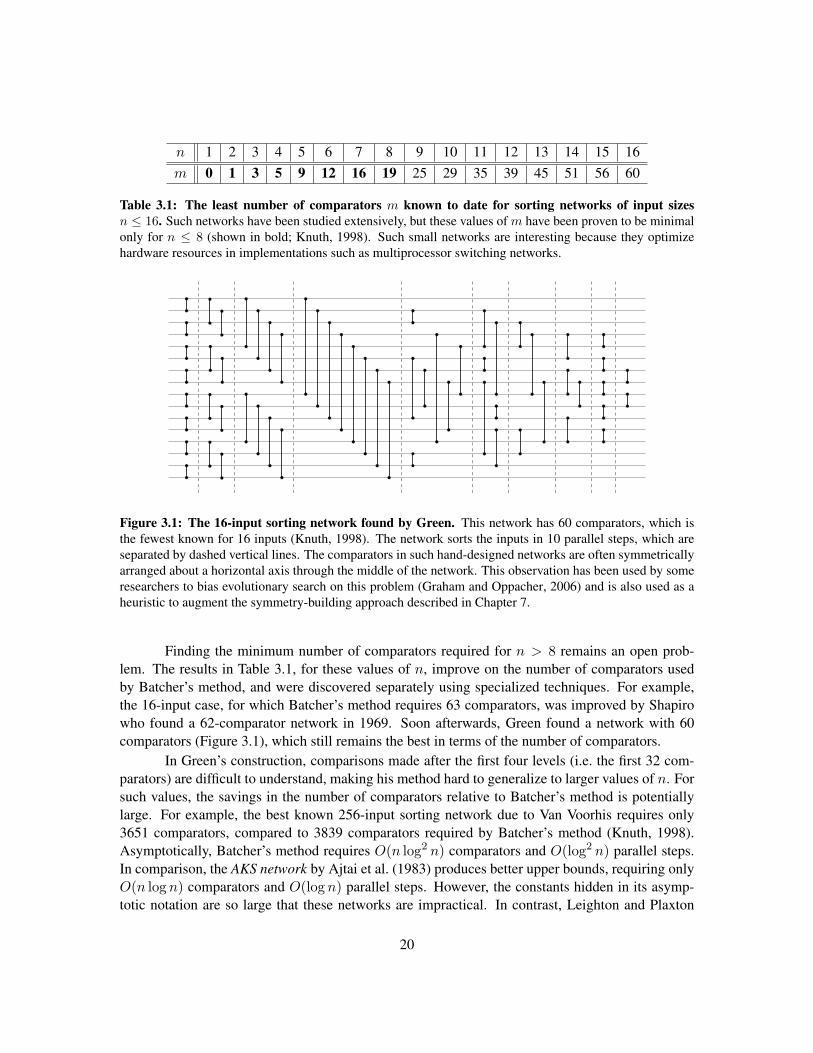
Figure 3.1: The 16-input sorting network found by Green. This network has 60 comparators, which isthe fewest known for 16 inputs (Knuth, 1998). The network sorts the inputs in 10 parallel steps, which areseparated by dashed vertical lines. The comparators in such hand-designed networks are often symmetricallyarranged about a horizontal axis through the middle of the network. This observation has been used by someresearchers to bias evolutionary search on this problem (Graham and Oppacher, 2006) and is also used as aheuristic to augment the symmetry-building approach described in Chapter 7.

Finding the minimum number of comparators required for n > 8 remains an open prob-lem. The results in Table 3.1, for these values of n, improve on the number of comparators usedby Batcher’s method, and were discovered separately using specialized techniques. For example,the 16-input case, for which Batcher’s method requires 63 comparators, was improved by Shapirowho found a 62-comparator network in 1969. Soon afterwards, Green found a network with 60comparators (Figure 3.1), which still remains the best in terms of the number of comparators.

In Green’s construction, comparisons made after the first four levels (i.e. the first 32 com-parators) are difficult to understand, making his method hard to generalize to larger values of n. Forsuch values, the savings in the number of comparators relative to Batcher’s method is potentiallylarge. For example, the best known 256-input sorting network due to Van Voorhis requires only3651 comparators, compared to 3839 comparators required by Batcher’s method (Knuth, 1998).Asymptotically, Batcher’s method requires O(n log2 n) comparators and O(log2 n) parallel steps.In comparison, the AKS network by Ajtai et al. (1983) produces better upper bounds, requiring onlyO(n log n) comparators and O(log n) parallel steps. However, the constants hidden in its asymp-totic notation are so large that these networks are impractical. In contrast, Leighton and Plaxton

20

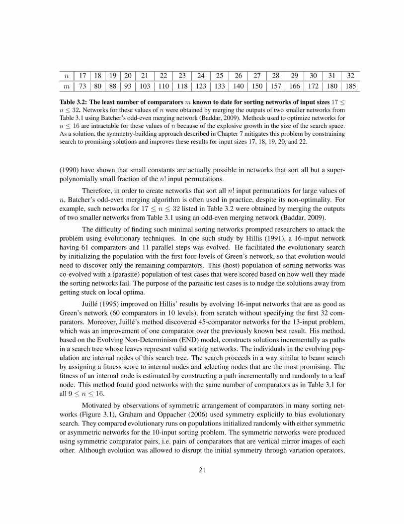
n 17 18 19 20 21 22 23 24 25 26 27 28 29 30 31 32m 73 80 88 93 103 110 118 123 133 140 150 157 166 172 180 185

Table 3.2: The least number of comparators m known to date for sorting networks of input sizes 17 ≤n ≤ 32. Networks for these values of n were obtained by merging the outputs of two smaller networks fromTable 3.1 using Batcher’s odd-even merging network (Baddar, 2009). Methods used to optimize networks forn ≤ 16 are intractable for these values of n because of the explosive growth in the size of the search space.As a solution, the symmetry-building approach described in Chapter 7 mitigates this problem by constrainingsearch to promising solutions and improves these results for input sizes 17, 18, 19, 20, and 22.

(1990) have shown that small constants are actually possible in networks that sort all but a super-polynomially small fraction of the n! input permutations.

Therefore, in order to create networks that sort all n! input permutations for large values ofn, Batcher’s odd-even merging algorithm is often used in practice, despite its non-optimality. Forexample, such networks for 17 ≤ n ≤ 32 listed in Table 3.2 were obtained by merging the outputsof two smaller networks from Table 3.1 using an odd-even merging network (Baddar, 2009).

The difficulty of finding such minimal sorting networks prompted researchers to attack theproblem using evolutionary techniques. In one such study by Hillis (1991), a 16-input networkhaving 61 comparators and 11 parallel steps was evolved. He facilitated the evolutionary searchby initializing the population with the first four levels of Green’s network, so that evolution wouldneed to discover only the remaining comparators. This (host) population of sorting networks wasco-evolved with a (parasite) population of test cases that were scored based on how well they madethe sorting networks fail. The purpose of the parasitic test cases is to nudge the solutions away fromgetting stuck on local optima.

Juille (1995) improved on Hillis’ results by evolving 16-input networks that are as good asGreen’s network (60 comparators in 10 levels), from scratch without specifying the first 32 com-parators. Moreover, Juille’s method discovered 45-comparator networks for the 13-input problem,which was an improvement of one comparator over the previously known best result. His method,based on the Evolving Non-Determinism (END) model, constructs solutions incrementally as pathsin a search tree whose leaves represent valid sorting networks. The individuals in the evolving pop-ulation are internal nodes of this search tree. The search proceeds in a way similar to beam searchby assigning a fitness score to internal nodes and selecting nodes that are the most promising. Thefitness of an internal node is estimated by constructing a path incrementally and randomly to a leafnode. This method found good networks with the same number of comparators as in Table 3.1 forall 9 ≤ n ≤ 16.

Motivated by observations of symmetric arrangement of comparators in many sorting net-works (Figure 3.1), Graham and Oppacher (2006) used symmetry explicitly to bias evolutionarysearch. They compared evolutionary runs on populations initialized randomly with either symmetricor asymmetric networks for the 10-input sorting problem. The symmetric networks were producedusing symmetric comparator pairs, i.e. pairs of comparators that are vertical mirror images of eachother. Although evolution was allowed to disrupt the initial symmetry through variation operators,

21

symmetric initialization resulted in higher success rates compared to asymmetric initialization. Asimilar heuristic is also utilized to augment the symmetry-building approach in Chapter 7.

Evolutionary approaches must verify that the solution network sorts all possible inputs cor-rectly. A naive approach is to test the network on all n! permutations of n distinct numbers. Abetter approach requiring far fewer tests utilizes the zero-one principle (Section 2.4) to reduce thenumber of test cases to 2n binary sequences. However, the increase in the number of test cases re-mains exponential and is a bottleneck in fitness evaluations. Therefore, some researchers have usedFPGAs to mitigate this problem by performing the fitness evaluations on a massively parallel scale(Korenek and Sekanina, 2005, Koza et al., 1998). In contrast, the symmetry-building approach inthis dissertation utilizes Boolean lattices to evaluate fitness efficiently.

3.4 Conclusion

Previous research on utilizing symmetry in evolutionary search have focused on indirect encodings,which are abstractions of development in nature. However, searching large design spaces efficientlyby utilizing symmetry to constrain search has been difficult because symmetries are difficult tospecify formally in such systems. The ENSO approach will addresses this issue by utilizing grouptheory to represent symmetry mathematically. This capability will then be utilized to evolve robustcontrollers for multilegged robots, a hard engineering problem that has been investigated since the1970s. Moreover, the general principle of utilizing symmetries to constrain search will be demon-strated on another challenging problem that has received considerable attention in the literature, i.e.designing minimal-size sorting networks.

22

Chapter 4

Evolving Modular Controllers

It is sometimes possible to constrain large search spaces by hand-designing symmetries. For ex-ample, the symmetries of modular neural network controllers for multilegged locomotion on flatground can be designed in this way (Sections 2.3 and 3.2). This chapter evaluates how effectivethe resulting search is by evolving walking behaviors for a simulated quadruped robot. Three typesof controllers were tested: (1) hand-designed controllers that serve as a baseline for performancecomparisons, (2) non-modular controllers unconstrained by symmetry (i.e. the parameters of theentire neural network are evolved at once), and (3) modular controllers constrained by symmetry(i.e. only one module is evolved and duplicated four times to produce the complex neural networkcontroller).

4.1 Quadruped Robot Model

The robot model resembles a table with a rectangular body supported by legs at the four corners(Figure 4.1). The legs are cylindrical with capped ends, and attached to the body by a hinge jointthat has a full 360° freedom of rotation. The axis of rotation of the joint is tilted to the side, causingthe rotating leg to trace a cone. The leg makes contact with the ground when it is at one edge of thecone. Forward or backward locomotion is achieved by coordinating the circular movements of theleg. The controller activates the simulated servo motor attached to each joint by specifying eitherthe desired joint angle or the angular velocity (in different experiments).

This model can be generalized and made more complex by adding more legs to the table orby using joints that have more degrees of freedom, such as a universal joint. Such more complexrobots will be used to test the scale-up properties of the approach in Sections 4.8 and 4.9.

4.2 Hand-Designed Controller

The hand-designed controller specifies the desired angular positions of the legs as functions oftime, coordinated so as to obtain a trot gait (Figure 1.1d). Plotted over time, the leg angles for thequadruped robot model produce sawtooth waveforms that all have the same period (Figure 4.2).

23

Figure 4.1: The quadruped robot model. The legs are attached to the body by hinge joints with axesof rotation tilted sideways, allowing the legs to make full circular rotation. Locomotion is achieved bycoordinating the circular movements of the legs. This model is a simple but physically realistic platform thatalso allows scaling up to more complex robots by adding more legs or by increasing the legs’ degrees offreedom.

The waveforms of the diagonal leg pairs are synchronous, and a half-period out of phase with theother pair. This gait is an effective base gait that occurs often in nature, and the evolved gaits can becompared with it.

4.3 Non-modular Controller

Figure 4.3a illustrates the non-modular neural network controller for the quadruped robot. Althougha variety of architectures are possible, this simple two-layer architecture was chosen to make a faircomparison to the symmetric modular controller. The inputs are the angular positions of the legjoints, and the outputs are the desired angular velocities of the legs. Each input unit is connected toall hidden units, but each output unit is connected only to two hidden units, which in turn send theiractivation exclusively to that output unit. The hidden and output units have sigmoidal activationfunctions with a bias and slope as parameters; the input units do not perform any computation.Since the genotype of the non-modular controller represents the entire network, all parameters ofthe network will have to be optimized through evolution.

A more general robot model having additional joint angles requires a network with addi-tional inputs and outputs to represent those angles. The number of hidden nodes will also need to beincreased to achieve better performance on more complex robots, thus increasing the search spaceand making the controller more difficult to optimize.

24

-240

-180

-120

-60

0

60

120

180

240

0 2 4 6 8 10

Leg

Join

t Ang

le (d

eg)

Time (s)

LF and RR RF and LR

Figure 4.2: Leg angles specified by the hand-designed controller. Plotted over time, these leg anglesproduce sawtooth waveforms, i.e. the legs rotate with constant angular velocity. The diagonal pairs of legsmove in unison, but each pair moves a half-period out of phase with the other pair, producing a trot gait.

(a) Non-modular controller network

(b) First module of the modular controller network

Figure 4.3: Genotypes of the non-modular and modular controller networks for the quadruped robotmodel. Inputs are the leg angles and outputs are the desired angular velocities. Both the non-modular andmodular networks have the same architecture. However, the genotype of the non-modular network containsthe entire network while that of the modular network contains only the first module. The full modular networkis constructed by replicating the first module with different permutations of the inputs.

25

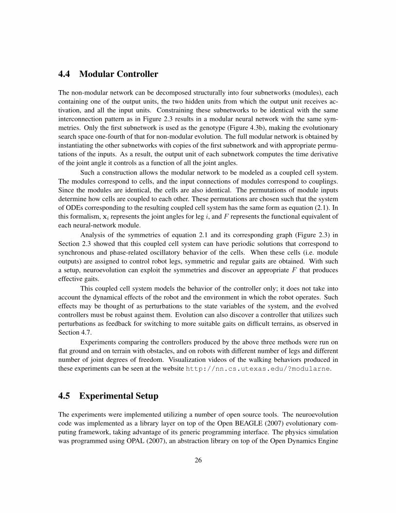
4.4 Modular Controller

The non-modular network can be decomposed structurally into four subnetworks (modules), eachcontaining one of the output units, the two hidden units from which the output unit receives ac-tivation, and all the input units. Constraining these subnetworks to be identical with the sameinterconnection pattern as in Figure 2.3 results in a modular neural network with the same sym-metries. Only the first subnetwork is used as the genotype (Figure 4.3b), making the evolutionarysearch space one-fourth of that for non-modular evolution. The full modular network is obtained byinstantiating the other subnetworks with copies of the first subnetwork and with appropriate permu-tations of the inputs. As a result, the output unit of each subnetwork computes the time derivativeof the joint angle it controls as a function of all the joint angles.

Such a construction allows the modular network to be modeled as a coupled cell system.The modules correspond to cells, and the input connections of modules correspond to couplings.Since the modules are identical, the cells are also identical. The permutations of module inputsdetermine how cells are coupled to each other. These permutations are chosen such that the systemof ODEs corresponding to the resulting coupled cell system has the same form as equation (2.1). Inthis formalism, xi represents the joint angles for leg i, and F represents the functional equivalent ofeach neural-network module.

Analysis of the symmetries of equation 2.1 and its corresponding graph (Figure 2.3) inSection 2.3 showed that this coupled cell system can have periodic solutions that correspond tosynchronous and phase-related oscillatory behavior of the cells. When these cells (i.e. moduleoutputs) are assigned to control robot legs, symmetric and regular gaits are obtained. With sucha setup, neuroevolution can exploit the symmetries and discover an appropriate F that produceseffective gaits.

This coupled cell system models the behavior of the controller only; it does not take intoaccount the dynamical effects of the robot and the environment in which the robot operates. Sucheffects may be thought of as perturbations to the state variables of the system, and the evolvedcontrollers must be robust against them. Evolution can also discover a controller that utilizes suchperturbations as feedback for switching to more suitable gaits on difficult terrains, as observed inSection 4.7.

Experiments comparing the controllers produced by the above three methods were run onflat ground and on terrain with obstacles, and on robots with different number of legs and differentnumber of joint degrees of freedom. Visualization videos of the walking behaviors produced inthese experiments can be seen at the website http://nn.cs.utexas.edu/?modularne.

4.5 Experimental Setup

The experiments were implemented utilizing a number of open source tools. The neuroevolutioncode was implemented as a library layer on top of the Open BEAGLE (2007) evolutionary com-puting framework, taking advantage of its generic programming interface. The physics simulationwas programmed using OPAL (2007), an abstraction library on top of the Open Dynamics Engine

26

http://nn.cs.utexas.edu/?modularne

(ODE, 2007). The Object-Oriented Graphics Rendering Engine (OGRE, 2007) library was used for3D visualization of the simulation.

The initial population of networks was created with connection weights chosen randomlyfrom the range [−2, 2), neuron biases set to 0, and neuron sigmoid slopes set to 1. Three typesof mutations were used, one for each of the above parameter types: (1) weight mutations, (2) biasmutations, and (3) slope mutations. All three types were implemented as Gaussian perturbations(with σ = 0.2), acting with a specified probability (0.5) on each of the parameters belonging tothat type. In each generation, an offspring was created by first selecting a parent in a two-waytournament and then applying exactly one of the three mutation types, chosen with equal probability.In addition, the network with the best fitness was copied without change to the next generation. Apopulation size of 200 was used in all experiments.

Each network was evaluated in a physically realistic simulation in which the network con-trolled the locomotion of a robot. When the robot was initially placed in the simulation environment,its longitudinal and lateral axes were aligned with the coordinate directions of the ground plane. Thesimulation was then carried out for one minute of simulated time with step size 0.01s, after whichthe fitness of the controller network was calculated as the maximum distance traveled by the robotalong either of the two coordinate dimensions (i.e. the Chebyshev distance; Murtagh, 2002). Thisfitness measure ensured that the evaluation of controller networks was fair even on the terrain withbumps arranged in concentric squares (Section 4.7). Although appropriate as a quantitative measureof performance, this measure does not capture how good the controllers are qualitatively. Therefore,the resulting gaits were also visualized and evaluated manually at the end of evolution to confirmthat the champion controller networks had good locomotive properties.

For all experiments, evolution was run for 500 generations and repeated 10 times, each timewith a different random number seed. The average and standard deviation of champion networkfitness over all experiments are plotted in Figure 4.4. The fitness of the hand-designed controlleris also plotted for comparison. This controller was obtained by manually implementing domainknowledge as well as by experimenting with gait periods similar to those produced by the modularcontrollers. The following sections discuss the results of each experiment in detail.

4.6 Walking on Flat Ground

In the first experiment, networks were evolved to control the simulated quadruped robot on flat ter-rain. The modular networks performed significantly better than the non-modular networks throughall generations, as illustrated in Figure 4.4a. This result implies that the robots with modular con-trollers are able to travel farther than those with non-modular controllers. Figure 4.4a also showsthat the modular controllers have higher fitness than the hand-designed controller. This result meansthat through evolution it was possible to discover more efficient or better tuned gaits than could bedesigned by hand.

When the locomotion of champion networks were visualized, another important benefit ofmodular evolution was revealed. The modular controllers produce regular gaits, such as pronk, pace,bound and trot, similar to those found in animals. Its hand-designed symmetries constrain the searchspace, making it easy to evolve such gaits (Section 2.3). In contrast, the non-modular networks

27

0

20

40

60

80

100

120

140

0 100 200 300 400 500

Fitn

ess

Generations

modularnon-modular

hand-designed

(a) Quadruped robot with hinge joints on flat terrain.

0

10

20

30

40

50

60

70

0 100 200 300 400 500

Fitn

ess

Generations

modularnon-modular

hand-designed

(b) Quadruped robot with hinge joints on obstacle terrain.

Figure 4.4: Performance of hand-designed, modular, and non-modular neuroevolution controllers ondifferent terrains and robot models. Bold lines are averages and the shaded regions on either side arestandard deviations obtained over 10 trials of evolution. The fitness of the hand-designed controller is alsoshown for reference. (a) Modular controllers perform significantly better than both non-modular and hand-designed controllers in the baseline experiment. (b) Performance gap between modular controllers and hand-designed controllers increases significantly when obstacles are added to the environment.

28

0

20

40

60

80

100

120

0 100 200 300 400 500

Fitn

ess

Generations

modularnon-modular

hand-designed

(c) Hexapod robot with hinge joints on flat terrain.

0

50

100

150

200

250

0 100 200 300 400 500

Fitn

ess

Generations

modularnon-modular

hand-designed

(d) Quadruped robot with universal joints on flat terrain.

Figure 4.4: (cont.) (c) Similarly, the performance gap increases significantly when number of legs is in-creased to six. (d) Likewise, performance gap increases significantly when an angular degree of freedomis added to each leg joint. These results demonstrate the advantage of modular evolution, i.e. search con-strained by symmetries, over non-modular evolution and hand-design in discovering controllers for multi-legged robots.

29

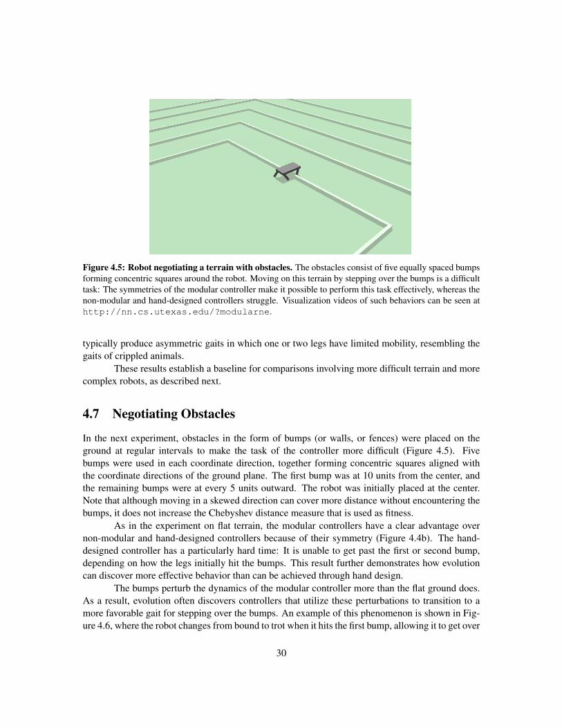
Figure 4.5: Robot negotiating a terrain with obstacles. The obstacles consist of five equally spaced bumpsforming concentric squares around the robot. Moving on this terrain by stepping over the bumps is a difficulttask: The symmetries of the modular controller make it possible to perform this task effectively, whereas thenon-modular and hand-designed controllers struggle. Visualization videos of such behaviors can be seen athttp://nn.cs.utexas.edu/?modularne.

typically produce asymmetric gaits in which one or two legs have limited mobility, resembling thegaits of crippled animals.

These results establish a baseline for comparisons involving more difficult terrain and morecomplex robots, as described next.

4.7 Negotiating Obstacles

In the next experiment, obstacles in the form of bumps (or walls, or fences) were placed on theground at regular intervals to make the task of the controller more difficult (Figure 4.5). Fivebumps were used in each coordinate direction, together forming concentric squares aligned withthe coordinate directions of the ground plane. The first bump was at 10 units from the center, andthe remaining bumps were at every 5 units outward. The robot was initially placed at the center.Note that although moving in a skewed direction can cover more distance without encountering thebumps, it does not increase the Chebyshev distance measure that is used as fitness.

As in the experiment on flat terrain, the modular controllers have a clear advantage overnon-modular and hand-designed controllers because of their symmetry (Figure 4.4b). The hand-designed controller has a particularly hard time: It is unable to get past the first or second bump,depending on how the legs initially hit the bumps. This result further demonstrates how evolutioncan discover more effective behavior than can be achieved through hand design.

The bumps perturb the dynamics of the modular controller more than the flat ground does.As a result, evolution often discovers controllers that utilize these perturbations to transition to amore favorable gait for stepping over the bumps. An example of this phenomenon is shown in Fig-ure 4.6, where the robot changes from bound to trot when it hits the first bump, allowing it to get over

30

http://nn.cs.utexas.edu/?modularne

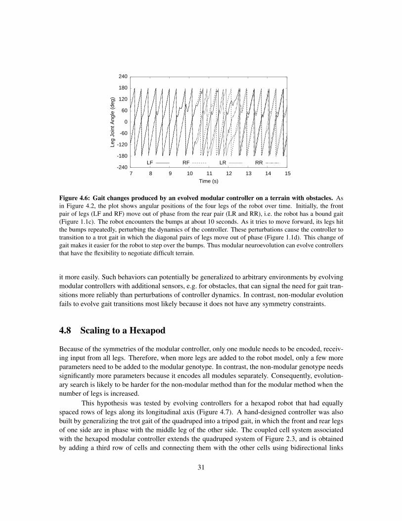
-240

-180

-120

-60

0

60

120

180

240

7 8 9 10 11 12 13 14 15

Leg

Join

t Ang

le (d

eg)

Time (s)

LF RF LR RR

Figure 4.6: Gait changes produced by an evolved modular controller on a terrain with obstacles. Asin Figure 4.2, the plot shows angular positions of the four legs of the robot over time. Initially, the frontpair of legs (LF and RF) move out of phase from the rear pair (LR and RR), i.e. the robot has a bound gait(Figure 1.1c). The robot encounters the bumps at about 10 seconds. As it tries to move forward, its legs hitthe bumps repeatedly, perturbing the dynamics of the controller. These perturbations cause the controller totransition to a trot gait in which the diagonal pairs of legs move out of phase (Figure 1.1d). This change ofgait makes it easier for the robot to step over the bumps. Thus modular neuroevolution can evolve controllersthat have the flexibility to negotiate difficult terrain.

it more easily. Such behaviors can potentially be generalized to arbitrary environments by evolvingmodular controllers with additional sensors, e.g. for obstacles, that can signal the need for gait tran-sitions more reliably than perturbations of controller dynamics. In contrast, non-modular evolutionfails to evolve gait transitions most likely because it does not have any symmetry constraints.

4.8 Scaling to a Hexapod

Because of the symmetries of the modular controller, only one module needs to be encoded, receiv-ing input from all legs. Therefore, when more legs are added to the robot model, only a few moreparameters need to be added to the modular genotype. In contrast, the non-modular genotype needssignificantly more parameters because it encodes all modules separately. Consequently, evolution-ary search is likely to be harder for the non-modular method than for the modular method when thenumber of legs is increased.

This hypothesis was tested by evolving controllers for a hexapod robot that had equallyspaced rows of legs along its longitudinal axis (Figure 4.7). A hand-designed controller was alsobuilt by generalizing the trot gait of the quadruped into a tripod gait, in which the front and rear legsof one side are in phase with the middle leg of the other side. The coupled cell system associatedwith the hexapod modular controller extends the quadruped system of Figure 2.3, and is obtainedby adding a third row of cells and connecting them with the other cells using bidirectional links

31

Figure 4.7: The hexapod robot model. This model is obtained by extending the quadruped in Figure 4.1with a third row of legs. It is used to test how well the different methods for designing controllers scale-up torobots with more legs.

(Figure 4.8). The resulting cell system has two types of symmetries: (1) swapping of the left andright columns of cells, and (2) cycling of the rows of cells either up or down.

Fitness of the modular and non-modular controllers in this experiment are plotted in Fig-ure 4.4c. The modular controllers now outperform the non-modular and hand-designed controllerswith a wider performance gap than in the quadruped case in Figure 4.4a. The non-modular con-trollers perform at the same level as the hand-designed controllers, possibly because they only haveto get a few legs moving in a coordinated fashion to make reasonable progress. On the other hand,the modular controllers produce gaits with symmetric leg movements, typically producing a lon-gitudinal wave pattern with same-row legs in phase or a half-period out of phase, which is muchmore effective and similar to the hexapod gaits in nature. Thus the symmetry constraints of modularevolution make it possible to scale up better than non-modular evolution when more legs are addedto the robot.

4.9 Scaling to Universal Joints

The robot can also be made more complex and more difficult to control by increasing the number ofangles that has to be controlled in each leg. That is, while the legs trace a cone in the previous robotmodels, a more challenging model would require controlling the forward-backward (longitudinal)and sideways (lateral) rotations of the legs separately. Since the controller inputs are the joint angles,the number of input connection weights increases correspondingly. This increase is limited to thesingle genotype module for modular networks, while it gets multiplied by the number of joints fornon-modular networks. Again, because of the large number of extra parameters that non-modularevolution has to search, finding a good controller is likely to be harder for non-modular than formodular evolution.

32

1 2

3 4

LeftFront

LeftMiddle

RightMiddle

RightFront

5 6LeftRear

RightRear

to/from cells 1 and 2

to/from cells 5 and 6

Figure 4.8: Graph of the coupled cell system for the hexapod robot in Figure 4.7. This system extendsthe quadruped system of Figure 2.3 by adding a third row of cells and connecting them with the other cellsusing bidirectional links. The resulting symmetries make the graph invariant to (1) swapping the left and rightcolumns of cells and (2) cycling the rows of cells up or down. These symmetries constrain the oscillations ofthe system, making it possible to evolve effective hexapod gaits similar to those in nature.

The final experiment tested this hypothesis by replacing each hinge joint of the quadrupedrobot with a universal (hip) joint. This change in the robot model doubles the number of degreesof freedom of each joint and, consequently, the number of controller inputs. The forward-backwardrotation is limited to 30° in both directions and the sideways rotation from vertical to 45° outwards.The hand-designed controller is generalized to this setup by adding signals for the lateral angle ofeach leg such that it is a quarter-period out of phase with its longitudinal angle, producing a trotgait.

The above hypothesis is confirmed by Figure 4.4d. The performance gap between modu-lar and non-modular evolution has widened significantly: Modular evolution now performs nearlyfour times better than non-modular evolution, and also slightly better than the hand-designed con-troller. Visualizing the gaits reveals that non-modular controllers typically produce gaits resemblingseverely crippled animals, with nearly all their legs appearing disabled and poorly coordinated.These robots often have sideways moving gaits and may have certain joint angles locked in a fixedposition. The modular controllers, on the other hand, typically produce regular trot gaits that achievehigh fitness.

Thus unlike non-modular evolution, modular evolution scales up well when the robot legsare made more complex. These results demonstrate that utilizing symmetries to constrain the searchspace makes it possible to scale up evolutionary search to more complex robots.

33

4.10 Conclusion

This chapter showed how the symmetries of modular controllers constrain evolutionary search,reducing the number of parameters that need to be optimized and thus making it possible to findeffective solutions. These symmetries were hand-designed to make it possible to evolve commonquadruped gaits found in nature such as pronk, pace, bound, and trot. The modular controllers alsoevolved the ability to change gaits in response to changes in the environment and to scale well tomore complex robot morphologies. In contrast, the unconstrained search of non-modular evolutionfailed to evolve effective controllers. However, designing symmetries by hand to constrain searchin this manner is not always possible, making it necessary to evolve the symmetries as well, as willbe discussed in the next chapter.

34

Chapter 5

Evolving Controller Symmetries

As the last chapter demonstrated, utilizing symmetries to constrain the search space makes it pos-sible to evolve effective solutions that are otherwise difficult or impossible to find. However, it isnot always possible to determine the appropriate symmetry analytically. For example, the hand-designed symmetries utilized in the last chapter are no longer appropriate when the robot is walkingon an incline, because the physics is different. Continuing in the robot control domain, this chapterextends modular neuroevolution to evolve symmetries as well. The key insight is to utilize grouptheory to keep the search space constrained to promising solutions while making it possible forevolution to explore different symmetries by breaking symmetry systematically.

5.1 Symmetry-Breaking Approach (ENSO)

This approach, called Evolution of Network Symmetry and mOdularity (ENSO), evolves both thesymmetries and the weights of modular neural networks simultaneously. ENSO represents the mod-ules and the connections between the modules as vertices and edges of a completely colored graph(Section 2.2). Since such graphs have an ordering induced by the subgroup lattice of their automor-phism groups, ENSO evolves symmetries by traversing this lattice from top to bottom. As a result,it searches the space of symmetries systematically from the most symmetric to the least symmet-ric, breaking symmetry minimally in each step to constrain search to promising graphs. Moreover,ENSO searches the space of network weights for each subgroup visited in the lattice. Therefore,evolving the graph representations of such modular networks consists of two components: (1) evolv-ing the symmetries of the module interconnection graph and (2) evolving the connection weightswithin and between modules. These components are described below.

5.1.1 Symmetry Evolution

In order to evolve a network with n modules, ENSO initializes a population of maximally symmet-ric, completely colored graphs with vertex set V = {1, 2, . . . , n}, that is, graphs of automorphismgroup Sn. These graphs have only two colors: All vertices are of one color while all edges are of theother color. Vertices and edges with the same color have the same set of neural network parameters

35

and are therefore considered identical. Therefore, each graph in the initial population represents amodular neural network with identical modules and identical connections between the modules.

ENSO computes the subgroup lattice of Sn and the orbital partitions for each subgroup inthe lattice at the beginning of evolution using the GAP (2007) software. During evolution, ENSOutilizes this lattice to mutate the coloring of graphs, thus breaking their symmetry. Each such colormutation creates a new graph coloring from the orbital partition of a randomly chosen successor inthe subgroup lattice; that is, the automorphism group of the mutated graph is a random maximalsubgroup of the automorphism group of the original graph.

ENSO organizes the colors created by successive color mutations as a tree. Each tree is agenotype for evolution. The leaf colors of the tree specify the complete coloring of a graph, whichis the phenotype that is constructed from the genotype. Each genotype tree of the initial populationhas two leaf nodes, one representing the color of vertices and the other representing the color ofedges (Figure 5.1a). These two leaf nodes are the children of a root node that represents a dummycolor.

Thus each node in the genotype tree represents a particular color c. Second, it representsthe set Q of elements of V × V (i.e. the set of vertices or edges of the phenotype graph) that havethe color c. This representation is a bit string of length n2, where the bit position (i − 1)n + j isset to 1 if and only if the pair (i, j) is in Q. Third, the node stores the neural network parametersof these elements, i.e. the biases and connection weights of the module network (for each vertex) orthe connection weights between modules (for each edge).

The effect of a color mutation on the genotype tree is to partition the set of vertex andedge elements associated with one or more leaf nodes, creating a new child color for each partof the partition (Figure 5.1b). As a result, the colors of these elements change correspondinglyin the phenotype graph, i.e. some of the elements that were identical before the mutation are nolonger identical: A new (initially random) set of neural network parameters is associated with eachnew color. These color changes break the symmetry of the phenotype graph, i.e. it loses its colorinvariance under a subset of permutations that were its symmetries prior to the mutation.

Since the automorphism group of the mutated graph is a maximal subgroup of the auto-morphism group of the original graph, color mutations break symmetry in minimal increments.As a result, evolution searches the space of symmetries systematically by exploring more symmet-ric graphs before less symmetric ones. Creating new colors and parameters in the genotype treeduring this process increases the complexity of the genotype, that is, evolution searches in a low-dimensional space before it complexifies into a higher dimensional space. This approach allowsevolution to optimize solutions in a small search space, and elaborate on them by adding more di-mensions. Such complexification has been demonstrated to be useful in other methods for evolvingneural networks (Siebel and Sommer, 2007, Stanley and Miikkulainen, 2004). Complexificationalso means that simpler solutions are preferred over more complex solutions, thus conforming tothe principle of Occam’s razor, which often results in more robust neural networks (Fahlman andLebiere, 1990, le Cun et al., 1990).

For each phenotype graph that ENSO produces in the above manner, it also evolves theneural network parameters associated with its colors to optimize the functionality of the network

36

PhenotypeGenotype

V x V:Params:

1111111111111111

p1,...,pk q1...,qm

Nil

Params: Params:

ColorMutation

(a)

(b)

Edges: 0111101111101110Vertices:1000010000100001

V x V:Params:

1111111111111111

p1,...,pk q1...,qm

Nil

Params: Params:Edges: 0111101111101110Vertices:1000010000100001

r1,...,rm s1...,smParams: Params:Edges: 0101101001101010Edges: 0010000110000100

x1 x2 x3 x4

y1

Module 1

Network module

x1 x2 x3 x4

y1

Module 1

1 2

3 4

1 2

3 4

Figure 5.1: Examples of genotype, phenotype, network module, and color mutation. ENSO uses a treeof colors as genotype (left). Each leaf of this tree has a unique color, and represents a set of vertices oredges of the phenotype graph (middle) that have the same parameter values. The vertices and edges of thephenotype graph represent the modules of a neural network and the connections between them (right). Theirparameters (stored in the genotype) consist of node biases and connection weights for each module network(vertex) and weights for each connection between modules (edge). Each module has a fixed architecture witha layer of hidden nodes fully connected to its inputs and outputs. A connection from another module (notshown) is implemented by fully connecting its input layer to the hidden layer of the target module. (a) At thebeginning of evolution, each genotype in the population represents a maximally symmetric phenotype graphwith automorphism group S4. All vertices of this graph have the same color (solid black, represented by theleaf on the left) and all its edges have the same color (orange with alternating dots and dashes, representedby the leaf on the right), implying that all modules are identical and all connections between them are alsoidentical. (b) A color mutation breaks the phenotype graph symmetry to D4, which is a maximal subgroup ofS4 (Figure 2.2). As a result, two child nodes are created for the node representing the set of edges, i.e. the setof edges is partitioned into two and each part is colored differently (dotted blue and dashed green). Since eachcolor is associated with a different combination of parameter values, the mutated phenotype graph representstwo types of connections between network modules. Such color mutations constrain symmetry search, andtogether with parameter mutations, make it possible to evolve symmetric modular neural networks efficiently.

modules and their interconnections. The structure of these modules and the evolution of networkparameters are described next.

5.1.2 Module Evolution

A fixed architecture is used for the neural network modules, each module consisting of a layer ofhidden nodes that are fully connected to inputs and outputs (Figure 5.1). Evolution optimizes twokinds of network parameters: (1) the scalar parameters of these modules, i.e. the connection weightsand node biases, which form the vertex parameters of the phenotype graph, and (2) the weights ofconnections between modules, which form the edge parameters of the phenotype graph. Moduleinterconnections are implemented by fully connecting the input layer of one module to the hiddenlayer of the other module (for instance, in a legged locomotion controller, such interconnections

37

allow the control module of one leg to receive the state of another leg as input). If modules are notconnected, then the corresponding graph edges are disabled using special binary edge parameters.

The vertex and edge parameters of the phenotype graph are stored in the genotype leafnodes. In the initial population, these parameters are initialized with random values in parameter-specific ranges specified by the experimenter. During evolution, ENSO mutates each of these pa-rameters probabilistically by perturbing them with Gaussian noise. When a parameter in a particulargenotype node is mutated, it affects all vertices and edges with that color. Thus, representing iden-tical elements by a single node in the genotype tree allows evolution to search the parameter spaceefficiently by making coordinated changes to the phenotype.

Symmetry and modules must be evolved together to find solution networks, making it nec-essary to mix parameter and color mutations. However, color mutations produce severe changes inthe phenotype, resulting in sudden changes in fitness that may cause the phenotype to be removedfrom the population. It is possible to determine how effective such structural changes are only afterenough parameter mutations have accumulated over evolutionary time. Therefore, color mutationsare given the opportunity to be optimized by creating population niches, similar in spirit to spe-ciation in the NEAT algorithm (Stanley and Miikkulainen, 2004) and to the evolution of structureand parameters at different time scales in the EANT/EANT2 algorithm (Siebel and Sommer, 2007).Individuals occupying a niche have the same phenotype symmetry and remain in the niche for acertain number of generations before they compete with the rest of the population. This number is alinear function of the size of the genotype, allowing individuals with more parameters to stay in theirniches longer. Protecting symmetry mutations using this niching mechanism improves evolutionaryperformance significantly.

Evolving the symmetries and parameters of modular neural networks in the above mannerconstrains search to explore promising regions of the subgroup lattice and corresponding parametercombinations. As a result, ENSO can find solutions to modular problems effectively, as demon-strated next.

5.2 Quadruped Controller

ENSO evolved modular controllers for the quadruped robot model described in Section 4.1. Al-though robots with more legs and complex legs can be used, this chapter focuses on symmetryevolution in challenging environments, and therefore uses only this simple model. As discussed inSection 4.4, the quadruped controller can be constructed using four modules, each with the samenetwork architecture (Figure 5.2a). Each module’s input is the joint angle of the leg it controls. Itcan be represented by the angle itself, or by the sine and cosine of the angle; the sine and cosine areactually more robust (because they are continuous), and will be used in the experiments on inclinedground. The module’s output is the desired angular velocity of that leg. The bias and slope of thehidden and output units and the weights of the internal connections of the module are the mutablevertex parameters of the phenotype graph (Section 5.1.2).

The phenotype graph represents the full controller network. It is obtained by connectingthe four modules to each other such that each module receives input from all the other modules(Figure 5.2b). The weights of these connections are the edge parameters of the phenotype graph.

38

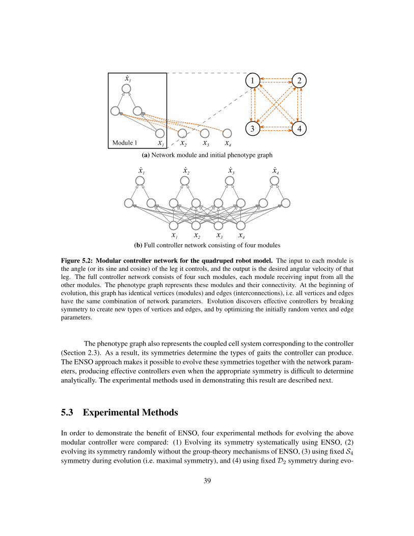
x1 x2 x3 x4

.x1

Module 1

1 2

3 4

(a) Network module and initial phenotype graph

x1 x2 x3 x4

.x1

.x2

.x3

.x4

(b) Full controller network consisting of four modules

Figure 5.2: Modular controller network for the quadruped robot model. The input to each module isthe angle (or its sine and cosine) of the leg it controls, and the output is the desired angular velocity of thatleg. The full controller network consists of four such modules, each module receiving input from all theother modules. The phenotype graph represents these modules and their connectivity. At the beginning ofevolution, this graph has identical vertices (modules) and edges (interconnections), i.e. all vertices and edgeshave the same combination of network parameters. Evolution discovers effective controllers by breakingsymmetry to create new types of vertices and edges, and by optimizing the initially random vertex and edgeparameters.

The phenotype graph also represents the coupled cell system corresponding to the controller(Section 2.3). As a result, its symmetries determine the types of gaits the controller can produce.The ENSO approach makes it possible to evolve these symmetries together with the network param-eters, producing effective controllers even when the appropriate symmetry is difficult to determineanalytically. The experimental methods used in demonstrating this result are described next.

5.3 Experimental Methods

In order to demonstrate the benefit of ENSO, four experimental methods for evolving the abovemodular controller were compared: (1) Evolving its symmetry systematically using ENSO, (2)evolving its symmetry randomly without the group-theory mechanisms of ENSO, (3) using fixed S4

symmetry during evolution (i.e. maximal symmetry), and (4) using fixed D2 symmetry during evo-

39

lution (as was done in Chapter 4). Although the four methods differ in how they evolve symmetry,they all evolve controller parameters in the same way as ENSO.

The first method (ENSO) initializes evolution with a population of maximally symmetricphenotype graphs (graph GA in Figure 2.1, having an S4 symmetry). Since they have identicalvertices and edges, their genotype trees have only two leaf colors, one representing vertex parame-ters and the other representing edge parameters. During evolution, color mutations break the initialgraph symmetry minimally to create new types of vertices and edges, and parameter mutationsoptimize the initially random vertex and edge parameters.

The second method (random symmetry) initializes evolution in the same way as above, butcolor mutations change the color of vertices and edges of the phenotype graph randomly. Eachsuch mutation chooses a random number of genotype leaf colors with probability proportional tothe size of the set of vertex or edge elements associated with those colors. Each of these colors isthen split into a random number of child colors corresponding to the subsets of elements producedby recursively partitioning the original set of elements. Like ENSO, these color mutations breakgraph symmetry, but unlike ENSO, they do not use group theory and therefore do not explore thesubgroup lattice systematically (Figure 2.2). Consequently, the resulting symmetry break may notbe minimal, producing larger changes in symmetry than ENSO. Therefore, this method is likely tobe less evolvable and is likely to perform worse than ENSO, i.e. it is unlikely to constrain symmetrysearch as effectively as ENSO.

The third method initializes evolution in the same way as the above two methods, i.e. withgraphs of S4 symmetry. However, it does not break this initial symmetry during evolution, andapplies only parameter mutations to the phenotype graphs. Therefore, it is a good baseline forcomparing with the above methods, making it possible to identify performance improvements dueto symmetry evolution.

The fourth method also evolves only parameters, keeping the symmetry of the phenotypegraphs fixed, but these graphs haveD2 symmetry (graphGB in Figure 2.1) instead of S4. This sym-metry is the same hand-designed symmetry utilized in Chapter 4 to evolve quadruped controllers.Thus this experiment forms a second comparison baseline for determining whether symmetry evo-lution can find more appropriate symmetries than those found through mathematical analysis.

Experiments comparing these four methods for evolving quadruped controllers were per-formed on flat ground and on inclined ground, as described next. The source code for these experi-ments is available from the website http://nn.cs.utexas.edu/?enso-code.

5.4 Experimental Setup

As with the experiments in Chapter 4, the initial population of controllers had connection weightsset randomly from the range [−2, 2), neuron biases set to 0, and neuron sigmoid slopes set to 1.Parameter mutations were implemented as Gaussian perturbations (with σ = 0.2) acting with aspecified probability (0.5) on each parameter. All edges were enabled in the phenotype graphsof the initial controllers, and mutations toggled them with a specified probability (0.1). In eachgeneration, an offspring was created by first selecting a parent in a two-way tournament, and thenapplying either a parameter mutation, an edge-toggle mutation, or a color mutation. Parameter

40

http://nn.cs.utexas.edu/?enso-code

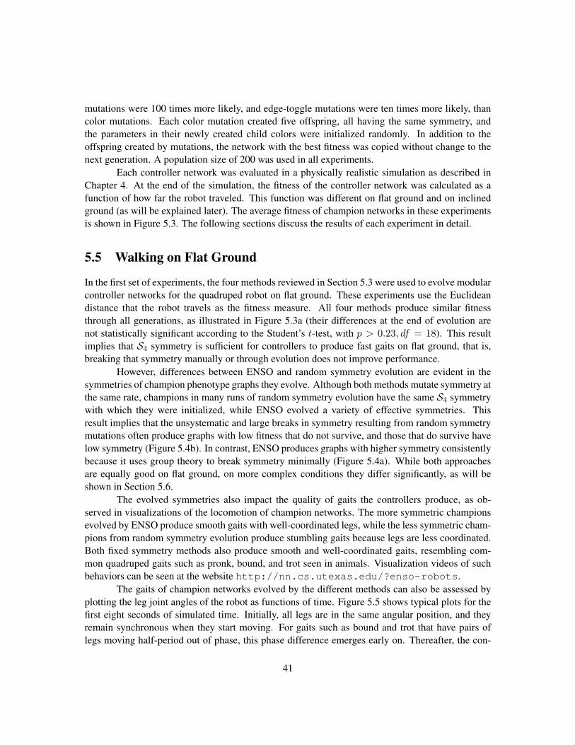
mutations were 100 times more likely, and edge-toggle mutations were ten times more likely, thancolor mutations. Each color mutation created five offspring, all having the same symmetry, andthe parameters in their newly created child colors were initialized randomly. In addition to theoffspring created by mutations, the network with the best fitness was copied without change to thenext generation. A population size of 200 was used in all experiments.

Each controller network was evaluated in a physically realistic simulation as described inChapter 4. At the end of the simulation, the fitness of the controller network was calculated as afunction of how far the robot traveled. This function was different on flat ground and on inclinedground (as will be explained later). The average fitness of champion networks in these experimentsis shown in Figure 5.3. The following sections discuss the results of each experiment in detail.

5.5 Walking on Flat Ground

In the first set of experiments, the four methods reviewed in Section 5.3 were used to evolve modularcontroller networks for the quadruped robot on flat ground. These experiments use the Euclideandistance that the robot travels as the fitness measure. All four methods produce similar fitnessthrough all generations, as illustrated in Figure 5.3a (their differences at the end of evolution arenot statistically significant according to the Student’s t-test, with p > 0.23, df = 18). This resultimplies that S4 symmetry is sufficient for controllers to produce fast gaits on flat ground, that is,breaking that symmetry manually or through evolution does not improve performance.

However, differences between ENSO and random symmetry evolution are evident in thesymmetries of champion phenotype graphs they evolve. Although both methods mutate symmetry atthe same rate, champions in many runs of random symmetry evolution have the same S4 symmetrywith which they were initialized, while ENSO evolved a variety of effective symmetries. Thisresult implies that the unsystematic and large breaks in symmetry resulting from random symmetrymutations often produce graphs with low fitness that do not survive, and those that do survive havelow symmetry (Figure 5.4b). In contrast, ENSO produces graphs with higher symmetry consistentlybecause it uses group theory to break symmetry minimally (Figure 5.4a). While both approachesare equally good on flat ground, on more complex conditions they differ significantly, as will beshown in Section 5.6.

The evolved symmetries also impact the quality of gaits the controllers produce, as ob-served in visualizations of the locomotion of champion networks. The more symmetric championsevolved by ENSO produce smooth gaits with well-coordinated legs, while the less symmetric cham-pions from random symmetry evolution produce stumbling gaits because legs are less coordinated.Both fixed symmetry methods also produce smooth and well-coordinated gaits, resembling com-mon quadruped gaits such as pronk, bound, and trot seen in animals. Visualization videos of suchbehaviors can be seen at the website http://nn.cs.utexas.edu/?enso-robots.

The gaits of champion networks evolved by the different methods can also be assessed byplotting the leg joint angles of the robot as functions of time. Figure 5.5 shows typical plots for thefirst eight seconds of simulated time. Initially, all legs are in the same angular position, and theyremain synchronous when they start moving. For gaits such as bound and trot that have pairs oflegs moving half-period out of phase, this phase difference emerges early on. Thereafter, the con-

41

http://nn.cs.utexas.edu/?enso-robots

0

20

40

60

80

100

120

0 100 200 300 400 500

Fitn

ess

Generations

ENSORandom symmetryFixed D2 symmetryFixed S4 symmetry

(a) Quadruped robot on flat ground

0

10

20

30

40

50

60

70

0 100 200 300 400 500

Fitn

ess

Generations

ENSORandom symmetryFixed D2 symmetryFixed S4 symmetry

(b) Quadruped robot on inclined ground

Figure 5.3: Performance of controllers evolved using ENSO, random symmetry breaking, fixed S4

symmetry, and fixed D2 symmetry methods on flat and inclined ground. The plots are averages over tentrials of evolution. (a) On flat ground, all four methods perform similarly and achieve the same high level offitness because many symmetries (including the hand-designed ones) can produce effective gaits in this case.(b) On inclined ground, however, both symmetry evolution methods perform better than the hand-designedsymmetries because the best symmetries are difficult for humans to conceive. Moreover, the group-theoreticsearch approach of ENSO constrains search to more promising symmetries than the random search approach,thereby finding significantly better solutions.

42

1 2

3 4

1 2

3 4

1 2

3 4= {(), (1243), (14), (1342), (14)(23), (23), (13)(24), (12)(34)}

D4 = {(), (12)(34), (13)(24), (14)(23)}

D2Z4 = {(), (12)(34), (1324), (1423)}

(a) ENSO (minimal symmetry breaking)

1 2

3 4

1 2

3 4

1 2

3 4S4 {e}{e}

(b) Random symmetry breaking evolution

Figure 5.4: Phenotype graphs of typical champion networks evolved by ENSO and random symmetryevolution on flat ground. (a) The group theory mechanisms used in ENSO for minimal symmetry breakingbiases evolution to produce phenotype graphs with high symmetry. Consequently, the robots they controlhave well-coordinated legs and smooth gaits. (b) In contrast, breaking symmetry randomly often produceslarge changes in symmetry that are deleterious and therefore do not survive. As a result, the champions ofmany evolutionary runs retain their initial S4 symmetry (left graph). Other champions such as the middle andright graphs have low symmetry that produce less coordinated, stumbling gaits.

trollers maintain synchronicity and phase relations between the legs. Well-coordinated gaits resultfor ENSO and the two fixed symmetry methods. However, random symmetry evolution typicallyproduces gaits that have the following two flaws: (1) legs are not well synchronized (e.g. the tworear legs in Figure 5.5b) and (2) phase difference between legs does not divide the period evenly(e.g. phase difference between the front and rear leg pairs in Figure 5.5b). The resulting weakcoordination of the legs produces the stumbling effect mentioned above, and seen in the videos.

To sum, although all methods produce gaits that are equally effective, ENSO’s solutions aremore symmetric and more smooth. Such a bias is a major advantage in more challenging environ-ments, as described next.

43

-240

-180

-120

-60

0

60

120

180

240

0 1 2 3 4 5 6 7 8

Leg

Join

t Ang

le (d

eg)

Time (s)

RF LF RR LR

(a) ENSO (bound gait)

-240

-180

-120

-60

0

60

120

180

240

0 1 2 3 4 5 6 7 8

Leg

Join

t Ang

le (d

eg)

Time (s)

RF LF RR LR

(b) Random symmetry evolution (gait resembling bound)

Figure 5.5: Example gaits of champion networks evolved by the different methods on flat ground. Thegraphs show the joint angles of the four legs of the robot in the first eight seconds of simulated time. Theplot for ENSO was produced using the left phenotype graph in Figure 5.4a and that for random symmetryevolution was produced using the middle phenotype graph in Figure 5.4b. When the controllers reach a steadystate, they maintain synchronicity and phase relations between legs. ENSO and the two fixed-symmetrymethods evolve controllers that produce the well-defined gaits illustrated in Figure 1.1. However, randomsymmetry evolution typically evolves controllers that produce lesser-quality gaits. For example, in the bound-like gait of (b), the rear legs are poorly synchronized and the phase difference between the front and rear legpairs is less than half-period. As a result, this gait is not as smooth as the gaits produced by ENSO and thefixed symmetry methods. Such smoothness is a major advantage in more challenging environments, as seenin Figure 5.7.

44

-240

-180

-120

-60

0

60

120

180

240

0 1 2 3 4 5 6 7 8

Leg

Join

t Ang

le (d

eg)

Time (s)

RF LF RR LR

(c) Evolution with fixed S4 symmetry (pronk gait)

-240

-180

-120

-60

0

60

120

180

240

0 1 2 3 4 5 6 7 8

Leg

Join

t Ang

le (d

eg)

Time (s)

RF LF RR LR

(d) Evolution with fixed D2 symmetry (trot gait)

Figure 5.5: (cont.)

5.6 Walking on Inclined Ground

In the second set of experiments, the ground was rotated about the longitudinal coordinate directionof the robot by 20◦ to make the task of the controller more difficult. The fitness measure is thedistance the robot travels along the longitudinal coordinate minus the distance it travels along thelateral coordinate. This measure encourages evolution to find controllers that move the robot for-ward in a straight line. Thus, the robot must walk across the incline without climbing up or down,while avoiding the risk of tipping over or slipping down the incline.

Since the robot is the same as before with no morphological changes, the same hand-designed symmetries should apply. However, when the robot is on inclined ground, the directionof gravity is not aligned with its plane of symmetry, thus breaking the symmetry of its dynamics

45

in a way that is difficult for a human designer to take into account. As a result, the appropriatecontroller symmetries for this task are expected to be different from those needed for walking onflat ground. Therefore, this task is a good test case to determine whether the fixed symmetry meth-ods can evolve effective controllers when appropriate symmetries are difficult to design by hand.Moreover, the task will evaluate whether ENSO is more effective than random symmetry evolutionat finding those symmetries.

The results of these experiments are shown in Figure 5.3b. ENSO produces significantly bet-ter fitness than random symmetry evolution (according to the Student’s t-test, with p < 0.002, df =18), which in turn produces significantly better fitness than evolution of fixed D2 symmetry (p <0.04, df = 18). The differences between the two fixed-symmetry methods are not statisticallysignificant (p > 0.13, df = 18). Since the only algorithmic difference between ENSO and ran-dom symmetry evolution is the way symmetries are broken, these results demonstrate that thegroup-theoretic symmetry mutations of ENSO are significantly better at evolving the appropriatesymmetries than random symmetry mutations, i.e. ENSO’s minimal symmetry breaking approachconstrains search to promising symmetries more effectively. In addition, the results demonstratethat finding these symmetries is crucial for evolving effective controllers, since fixed symmetryevolution utilizing hand-designed symmetries performs significantly worse.

In this more challenging task, the phenotype graphs that ENSO evolves (Figure 5.6a) areoften less symmetric than those it evolves on flat ground (Figure 5.4a). In particular, it evolvesgraphs that have two vertex colors, and therefore the corresponding controllers have two types ofmodules, making it possible for evolution to implement a different control function in each module.Different modules can implement different leg behaviors useful for walking effectively on inclinedground. Typically, two (or three) legs of the same module type remain nearly stationary to providethe support necessary for maintaining the robot’s forward orientation, while the other legs make afull circle, propelling the robot forward without slipping.

The unsystematic symmetry mutations of random symmetry evolution are typically detri-mental on inclined ground as well, and as a result many of the champion phenotype graphs retaintheir original S4 symmetry (Figure 5.6b). However, occasionally random symmetry evolution man-ages to discover symmetries that generate faster gaits than the fixed-symmetry methods. The gaitsthe fixed symmetry methods produce on inclined ground are similar to those they produce on flatground because their gaits are constrained by symmetry. However, these gaits are not as effectiveon inclined ground, and the gaits discovered by ENSO are faster.

Figure 5.7 illustrates the above observations by plotting leg angles of typical evolved con-trollers. The controller evolved by ENSO generates two types of waveforms, each correspondingto a different type of module and representing a different leg behavior. The first module type con-trols only the right rear leg, which powers the robot’s forward motion. The second module typecontrols all the other legs and helps maintain the robot’s orientation. The controllers for the otherthree methods have only one type of waveform because all legs are controlled by the same type ofmodule. As on flat ground, the gaits evolved by random symmetry mutations are less regular thanthose evolved by the other methods. The controller evolved with the fixed S4 symmetry producesa new gait that is different from the four gaits discussed in Figure 1.1; it is similar to the walk, i.e.legs are quarter-period separated in phase, while the controller evolved with fixed D2 symmetry

46

1 2

3 4

1 2

3 4

1 2

3 4S3 = {(), (124), (142),

(12), (14), (24)}Z3 = {(), (234), (243)}Z2 = {(), (14)(23)}

(a) ENSO (minimal symmetry breaking)

1 2

3 4

1 2

3 4

1 2

3 4S4 Z2 = {(), (14)} {e}

(b) Random symmetry breaking evolution

Figure 5.6: Phenotype graphs of typical champion networks evolved by ENSO and random symmetryevolution on inclined ground. (a) The graphs that produce effective gaits on inclined ground are often lesssymmetric than the graphs on flat ground (Figure 5.4a). They typically have two vertex colors, representingtwo types of controller modules that produce different leg behaviors for such gaits. (b) As on flat ground (Fig-ure 5.4b), random symmetry evolution produces many graphs with the initial S4 symmetry, which producesless effective gaits on inclined ground. Other graphs it produces can generate faster gaits, but they are oftenslower than the gaits produced by ENSO. Thus the systematic symmetry search of ENSO is more effectivewhen finding the right symmetry is more important.

produces a trot gait. Comparing the periods of the plotted gaits indicates that the gait evolved byENSO is faster than the other gaits.

Thus ENSO evolves more effective gaits on inclined ground than the other methods byfinding symmetries that are better suited to the incline. Since ENSO adapts the gaits better to theenvironment, they should generalize better to changes in the environment as well. This hypothesiswas tested by reducing the ground friction of the incline, as described next.

5.7 Generalization to Reduced Friction

Generalization of the champion controllers evolved by the different methods on inclined groundwere tested by reducing the friction coefficient of the ground by 25%; all other simulation parame-ters remained the same. Making the ground slippery in this manner makes it harder for the robots

47

-240

-180

-120

-60

0

60

120

180

240

0 2 4 6 8 10 12

Leg

Join

t Ang

le (d

eg)

Time (s)

RF LF RR LR

(a) ENSO

-240

-180

-120

-60

0

60

120

180

240

0 2 4 6 8 10 12

Leg

Join

t Ang

le (d

eg)

Time (s)

RF LF RR LR

(b) Random symmetry evolution

Figure 5.7: Example gaits of champion networks evolved by the different methods on inclined ground.The graphs show the joint angles of the four legs of the robot in the first twelve seconds of simulated time.The plot for ENSO was produced using the middle phenotype graph in Figure 5.6a, and it shows the twowaveforms corresponding to the two types of modules in the phenotype graph. The plot for random symmetryevolution was produced using the middle phenotype graph in Figure 5.6b, and it shows that this gait is lessregular than the gaits produced by the other methods. Plots (c) and (d) show that evolving with fixed S4 andD2 symmetries produce the same gaits as on flat ground. However, they are significantly slower than the gaitevolved by ENSO, as seen from the difference in gait periods.

48

-240

-180

-120

-60

0

60

120

180

240

0 2 4 6 8 10 12

Leg

Join

t Ang

le (d

eg)

Time (s)

RF LF RR LR

(c) Evolution with fixed S4 symmetry

-240

-180

-120

-60

0

60

120

180

240

0 2 4 6 8 10 12

Leg

Join

t Ang

le (d

eg)

Time (s)

RF LF RR LR

(d) Evolution with fixed D2 symmetry (trot gait)

Figure 5.7: (cont.)

to maintain their balance and orientation as they walk across the incline. However, controllers thatevolved effective gaits for the incline should be able to maintain acceptable performance.

Since the controllers evolved with fixed S4 and D2 symmetries and random symmetry mu-tations are ill-suited for inclines, the robot often ended up flipping over or moving downhill insteadof walking across the incline, i.e. such controllers generalize poorly to slippery inclines. In contrast,the controllers that ENSO evolved make the robot walk nearly straight across the incline, slippingonly a little. This behavior is possible because ENSO optimizes controllers to perform well oninclines, resulting in gaits that also generalize better. This type of generalization is crucial for trans-ferring the controllers that ENSO evolves in simulation to physical robots, as discussed in the nextchapter.

49

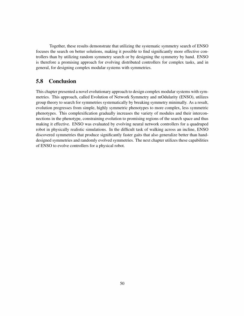
Together, these results demonstrate that utilizing the systematic symmetry search of ENSOfocuses the search on better solutions, making it possible to find significantly more effective con-trollers than by utilizing random symmetry search or by designing the symmetry by hand. ENSOis therefore a promising approach for evolving distributed controllers for complex tasks, and ingeneral, for designing complex modular systems with symmetries.

5.8 Conclusion

This chapter presented a novel evolutionary approach to design complex modular systems with sym-metries. This approach, called Evolution of Network Symmetry and mOdularity (ENSO), utilizesgroup theory to search for symmetries systematically by breaking symmetry minimally. As a result,evolution progresses from simple, highly symmetric phenotypes to more complex, less symmetricphenotypes. This complexification gradually increases the variety of modules and their intercon-nections in the phenotype, constraining evolution to promising regions of the search space and thusmaking it effective. ENSO was evaluated by evolving neural network controllers for a quadrupedrobot in physically realistic simulations. In the difficult task of walking across an incline, ENSOdiscovered symmetries that produce significantly faster gaits that also generalize better than hand-designed symmetries and randomly evolved symmetries. The next chapter utilizes these capabilitiesof ENSO to evolve controllers for a physical robot.

50

Chapter 6

From Simulation to Reality

The ultimate goal of evolving controllers in simulation is to transfer them to real robots. In orderto verify that ENSO can evolve controllers that transfer to the real world, I built a physical robot,similar to those targeted by the simulations, at the Cornell Computational Synthesis Lab (2010) ofProf. Hod Lipson. This chapter describes designing and building this robot and utilizing ENSO toevolve neural network controllers for it. The goal was to find out whether the robot would walksuccessfully and whether the gaits would be more robust against noise and faults than those thatcould be built by hand.

6.1 Evolving Controllers for Real Robots

It is possible to evolve controllers by evaluating their fitness directly on the real robot instead of insimulation (Floreano and Mondada, 1998, Hornby et al., 2000, Kohl and Stone, 2004b, Watson et al.,2002, Zykov et al., 2004, Section 3.2). However, performing thousands of such fitness evaluationsin hardware may be impractical for the following reasons (Mataric and Cliff, 1996). First, hardwareevaluations are slow, resulting in long evolutionary run times. Second, they cause wear and tear onthe robot, making hardware failures likely and user intervention to repair them necessary. Third, thecontrollers created by evolution through random variations may produce abnormal actuator signalsthat can crash or damage the robot.

Therefore, a good alternative is to evaluate controller fitness in simulation and then trans-fer only the final, evolved controller to the physical robot. However, transferring such controllersevolved in simulation to the physical robot is challenging (Brooks, 1992, Jakobi, 1998, Lipson et al.,2006, Mataric and Cliff, 1996). The main reason is that it is difficult to simulate physical propertiessuch as friction and sensor and actuator characteristics with high enough fidelity to reproduce thesimulated behaviors on real robots. In order to address this issue, researchers have developed severalmethods that improve the results of evolving in simulation by performing only a few experimentson the real robot.

A straightforward method is to fine-tune the controller behaviors evolved in simulation bycontinuing evolution on the real robot for a few more generations (Miglino et al., 1995, Nolfi et al.,1994). However, this method may be ineffective in correcting controller behaviors that have evolved

51

to exploit flaws in the simulation. A better alternative is to make such behaviors less likely to evolveby incorporating transfer experiments from the beginning of evolution, e.g. by utilizing a multi-objective evolutionary algorithm that optimizes both a task-dependent controller fitness as well as ameasure of how well the controller transfers from simulation to reality (Koos et al., 2010). In anygiven generation, this method chooses at most one controller based on behavioral diversity to beevaluated on the real robot, requiring only a small number of hardware evaluations.

Other methods utilize the information they gather from a few experiments on the real robotto build a more realistic simulator, typically in one of two ways: (1) Experiments are performedon the real robot before running evolution to collect samples of the real world by recording sensoractivations (Miglino et al., 1995, Nolfi et al., 1994). When controllers are evaluated later duringevolution, these samples are utilized to set the simulated sensor activations accurately. (2) Experi-ments are performed on the real robot during evolution to co-evolve the simulator and the controller,making an initially crude simulation more and more accurate (Bongard and Lipson, 2004, Brooks,1992, Zagal and Ruiz-Del-Solar, 2007).

In contrast to the above methods, the approach presented in this chapter bridges the simulation-reality gap by utilizing controllers that are robust to small discrepancies between simulation andreality. ENSO can evolve such controllers because they are coupled cell systems that provide the-oretical guarantees of robustness to such small discrepancies (Section 2.3). Therefore, simulationaccuracies sufficient for ENSO can be obtained easily by approximating the morphology and massdistribution of the real robot with cylindrical and rectangular blocks, without the need for any hard-ware experiments either before or during evolution (Section 6.3).

Evolving controllers in an accurate enough simulation is often insufficient to transfer themsuccessfully to the real world because of uncertainties such as in sensor activations and actuatorresponses. Researchers have demonstrated that evolution can adapt controllers to such uncertaintiesby modeling them as noise in the simulation (Gomez and Miikkulainen, 2004, Jakobi et al., 1995,Miglino et al., 1995). The same idea is utilized in this chapter to evolve controllers that are robustagainst uncertainties in how the motors respond to control signals. The controllers evolved in theresulting simulation transfer successfully to the physical robot, producing the same behaviors bothin simulation and on the physical robot. The design and fabrication of this robot are discussed next.

6.2 Parts and Design

The physical robot was designed with two constraints: (1) it must be similar to the model in Sec-tion 4.1 so that ENSO can evolve controllers for it in simulation without big modifications, and (2) itmust be possible to prototype it quickly with parts that can be purchased or fabricated easily. Whilesome parts of the robot such as the servo motors and the controller board to operate the motors wereavailable commercially, other parts such as its body and legs were custom-designed and fabricatedto fit the commercial parts.

Each leg of the robot is attached to a Dynamixel AX-12+ servo motor (Figure 6.1) manufac-tured by Robotis (2010). The AX-12+ provides angular position feedback, and can be made to rotatecontinuously by specifying the desired angular velocity, making it suitable for use with the architec-ture of neural network controllers discussed in previous chapters. The neural network controlling

52

SerialConnectors

Rotating output flange

Figure 6.1: Back and front views of the Dynamixel AX-12+ motor. Each motor’s rotating output flangeis attached to a robot leg. A quadruped robot therefore has four such motors and a hexapod has six, whichare connected in a daisy chain using serial connectors. One end of the daisy chain is plugged into a CM-2+microcontroller board (Figure 6.2) running an evolved neural network controller. This setup allows the neuralnetwork to communicate with all four motors and thus control the leg movements of the robot. Reprintedwith permission from Robotis (2010); annotations added.

the robot runs on a Robotis CM-2+ microcontroller circuit board (Figure 6.2), which provides aninterface to communicate with the Dynamixel motors through a daisy-chain serial connection.

The AX-12+ motors are mounted on a rectangular body using a wedge-shaped piece totilt their axes of rotation 20° from the vertical (Figure 6.3). The legs also slant 20° from theirrespective motor axes, making it possible for the robot to walk by rotating its legs continuously (aswas described in Section 4.1). The body, the wedge, and the leg were designed using SolidWorks(2010), a program for computer aided design. The body was then cut from acrylic using a lasercutter and the wedges and the legs were fabricated in an Objet Eden 260V (2010) rapid-prototyping3D printer. The circuit board is mounted on the top side of the body and is powered by a 12Vlithium-ion battery attached to its bottom side by Velcro.

Although the morphology and walking mechanism of this robot is similar to the model inprevious simulations, it has more parts and it is more complex. Therefore, the simulation wasextended to model the physical characteristics of the robot more accurately.

6.3 Extending the Simulation

The robot’s legs are still modeled as cylinders with capped ends, but its body is now assembledfrom several rectangular boxes that approximate its different parts (Figure 6.4). These cylinders andboxes have the same dimensions and the same relative angles as the corresponding parts in the realrobot. The leg angles used as controller input are measured from the same vertical leg positions.Moreover, densities are assigned to parts such that they have the same mass in both simulation andthe real robot. As a result, this simulation model has the same approximate morphology and massdistribution as the physical robot.

53

Power switch Serial jack(to PC)

Serialconnector

(to AX-12+)

ATmega128microcontroller

DC powerjack

Figure 6.2: Top and bottom views of the CM-2+ circuit board. The CM-2+ board uses an ATmega128microcontroller with 128KB flash memory and runs control programs for Dynamixel AX-12+ motors. Theevolved neural network controllers are expressed in the C language and cross compiled for the ATmega128using the GNU compiler toolchain. The compiled program is then downloaded to the CM-2+ via its RS-232serial jack. The CM-2+ executes this program when it is switched on, sending control instructions to theDynamixels connected in a daisy chain through its serial connector. Reprinted with permission from Robotis(2010); annotations added.

In addition to the morphology, the sensor and actuator characteristics of the AX-12+ motorsare also modeled. The motor can sense its angular position if it is in the [0, 300] degree range (Fig-ure 6.5). However, it does not give valid position feedback for angles between 300° and 360°. Sincethe neural network controllers require angular positions as inputs, the sensor reading is interpolatedwhen the motor is in this blind zone. In fact, the sensor reading is calculated the same way for allangles from an estimate of the angular velocity, which gets updated only when the angle is in thevalid range. Exponential smoothing is applied to this estimate to filter out noise and discontinu-ities caused by any discrepancy between the estimated and actual angular velocities when the motoremerges from the blind zone.

The response of the motor to the angular velocity control signals from the neural network ismore difficult to model accurately. In particular, the angular velocity of the motor drifts significantly

54

Figure 6.3: Assembled physical quadruped robot. The Dynamixel AX-12+ motors rotate the legs of therobot and are mounted on the four corners of its rectangular acrylic body, which has attachment points inthe middle for a future hexapod extension. The legs make 20° with the axis of rotation of their respectivemotors, tracing trace cones as they rotate. The motor axes also have a 20° sideways tilt from the vertical.As a result, rotating the legs raises and lowers them and can produce locomotion when they make contactwith the ground. A control program synchronizes the rotation of the legs to produce locomotion and runs onthe CM-2+ circuit board mounted on top of the body. The board is powered by a 12V lithium-ion batteryattached to the under-side of the body. Videos of experiments utilizing this robot can be seen at the websitehttp://nn.cs.utexas.edu/?enso-realrobots

Figure 6.4: Simulation of the physical quadruped robot. The simulation model in Section 4.1 was ex-tended to resemble the morphology and dynamics of the physical robot in Figure 6.3 more closely. The legsare modeled as capped cylinders and the other parts are approximated as rectangular boxes with the samedimensions. By assigning the weight of the corresponding parts to these shapes, this model represents theweight distribution of the physical robot with sufficient accuracy to simulate it realistically.

55

http://nn.cs.utexas.edu/?enso-realrobots

150°Position = 511

300~360°

Invalid Angle

300°Position = 1023

0°Position = 0

Figure 6.5: Angular position sensor readings of the Dynamixel AX-12+ motor. The angular position sen-sor of the motor provides an integer valued reading in the range [0, 1023] when the motor is in the [0, 300] de-gree range; angles outside this range produce invalid sensor readings and are therefore interpolated. Reprintedwith permission from Robotis (2010); annotations edited.

over time for a constant control signal. This stochastic drift can change the periodic trajectory ofthe controller, thus disrupting the gait of the robot. Such uncertainties can be handled by addingnoise to the simulation, making it possible for evolution to adapt the controllers suitably (Gomezand Miikkulainen, 2004, Lipson et al., 2006). Two types of Gaussian noise were added: The firsttype models fluctuations about the mean with standard deviation 2.5%. The second type of noisemodels drifts in the mean; it is therefore larger in magnitude (standard deviation 20%), but it isapplied only a few times during evaluation.

The motor’s inaccuracy in representing its angular position and velocity is also included inthe simulation. The motor represents both variables with an integer value in the range [0, 1023].Their precision in simulation is therefore downgraded from floating point precision to match the ac-tual precision. Moreover, the neural network controller reads the positions and updates the velocitiesat the same frequency in both simulation and the real robot.

The controller evolved in simulation in the above manner is transferred to the real robot byprogramming the CM-2+ circuit board with it, as will be described next.

6.4 Control Programs

The CM-2+ circuit board contains an ATmega128 CPU, which is an 8-bit microcontroller with128KB of on-chip programmable flash memory. It can run programs stored in its memory foractivating the motors of the robot. Therefore, the evolved neural network controller is converted toa C-language representation and is invoked from a control loop similar to that used in simulation for

56

1 2

3 4

= {(), (1243), (14), (1342), (14)(23), (23), (13)(24), (12)(34)}

D4

Figure 6.6: Phenotype graph of a champion neural network controller evolved by ENSO. This graphhas symmetry group D4, making it similar to the graphs that ENSO evolved in Chapter 5 for a simpler robotmodel. As a result, it produces a trot gait, and it transfers well from simulation to the real robot (Figure 6.7).

interfacing the network with the motors. This C program is then cross-compiled for the ATmega128using the GNU compiler toolchain and downloaded to the CM-2+ board through an RS-232 serialconnection.

This facility for writing control programs in C was also utilized to hand-code a baselinecontroller in order to compare hand-design with evolved controllers. The approach extends thehand-designed controller in Section 4.2: The neural network in the control loop is replaced witha PID controller of the leg angular velocities that utilizes feedback of leg positions. Thus, thehand-designed controller also benefits from the mechanism mentioned above for interpolating andsmoothing sensor readings of leg positions. It generates a sawtooth waveform for the desired legpositions as a function of time (Section 4.2) and uses this waveform as reference to compute errorsignals for PID control.

Experiments comparing this controller with evolved controllers are described in the follow-ing sections. The gaits produced by the evolved and hand-designed controllers were evaluated forwalking on flat ground (1) when all four legs of the robot are functional and (2) when one leg isdisabled to simulate a real-world motor failure. The controllers produced in the first experimentwere evaluated further for generalization by reducing the maximum speed of the motors and byinitializing one of the legs with a large error. In each experiment, generalization was also tested byplacing the robot on different surfaces. In each case, ENSO evolved controllers utilizing the sameexperimental setup and parameters as discussed in Section 4.5. Videos of these experiments can beseen at the website http://nn.cs.utexas.edu/?enso-realrobots.

6.5 All Legs Enabled

Figure 6.6 shows the phenotype graph of a champion neural network controller that ENSO evolvedto walk on flat ground utilizing the simulation model extended in this chapter. Its symmetry (D4) issimilar to that of the graphs that ENSO evolved in Chapter 5 for the simpler robot model. Therefore,it also produces a similar trot gait (Figure 6.7a), demonstrating that ENSO can evolve symmetriccontrollers producing symmetric gaits even for a more complex robot model that is more realistic.

57

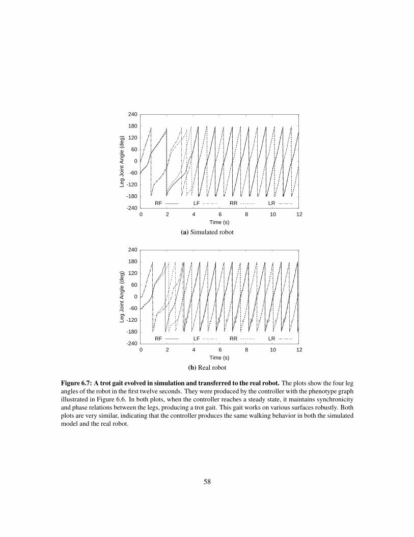
http://nn.cs.utexas.edu/?enso-realrobots

-240

-180

-120

-60

0

60

120

180

240

0 2 4 6 8 10 12

Leg

Join

t Ang

le (d

eg)

Time (s)

RF LF RR LR

(a) Simulated robot

-240

-180

-120

-60

0

60

120

180

240

0 2 4 6 8 10 12

Leg

Join

t Ang

le (d

eg)

Time (s)

RF LF RR LR

(b) Real robot

Figure 6.7: A trot gait evolved in simulation and transferred to the real robot. The plots show the four legangles of the robot in the first twelve seconds. They were produced by the controller with the phenotype graphillustrated in Figure 6.6. In both plots, when the controller reaches a steady state, it maintains synchronicityand phase relations between the legs, producing a trot gait. This gait works on various surfaces robustly. Bothplots are very similar, indicating that the controller produces the same walking behavior in both the simulatedmodel and the real robot.

58

-240

-180

-120

-60

0

60

120

180

240

0 2 4 6 8 10 12

Leg

Join

t Ang

le (d

eg)

Time (s)

RF LF RR LR

Figure 6.8: Trot gait produced by the hand-designed controller for the real robot. The plot shows thefour leg angles of the robot in the first twelve seconds. This controller keeps the legs synchronized witha reference waveform for a trot gait by applying PID control to correct small errors in leg positions. Suchcontrollers are difficult to design by hand in the general case.

Transferring this controller to the real robot reproduces the same gait (Figure 6.7b). It isrobust enough to walk smoothly in a straight line even on very different surfaces such as linoleumand carpet. These results demonstrate that ENSO can evolve controllers that transfer successfullyfrom simulation to real robots.

The hand-designed controller was also tested on the real robot with a reference waveformfor a trot gait having approximately the same period as the evolved controller (Figure 6.8). The legsare first positioned on the reference waveform so that there is no error for the controller to correctwhen it starts. Thereafter, the PID mechanism of the controller corrects small errors by speeding upor slowing down the legs to keep them aligned with the reference waveform. As a result, it producesa trot gait similar to the evolved controller. However, it is not as robust and does not generalize aswell as the evolved controller as demonstrated by the experiments discussed next.

6.6 Generalization to Reduced Motor Speed

The maximum leg angular velocity that the motors can produce depends on the conditions in whichthe robot operates. For example, it decreases when the input voltage to the motor decreases as aresult of e.g. low battery charge or temperature (Gao et al., 2002, Zhang et al., 2003). The challengefor the controller is to keep the legs synchronized and the robot walking effectively even in suchconditions. Both the hand-designed and evolved controllers were tested for their ability to generalizeto such conditions by reducing the maximum angular velocity that the motors produce.

The hand-designed controller fails, losing leg synchronization, even for a small (10%) re-duction in the maximum angular velocity (Figure 6.9a). It fails because the legs can no longer movefast enough to keep up with the reference waveform. Slowing down the waveform can correct the

59

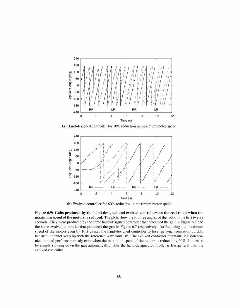
-240

-180

-120

-60

0

60

120

180

240

0 2 4 6 8 10 12

Leg

Join

t Ang

le (d

eg)

Time (s)

RF LF RR LR

(a) Hand-designed controller for 10% reduction in maximum motor speed

-240

-180

-120

-60

0

60

120

180

240

0 2 4 6 8 10 12

Leg

Join

t Ang

le (d

eg)

Time (s)

RF LF RR LR

(b) Evolved controller for 60% reduction in maximum motor speed

Figure 6.9: Gaits produced by the hand-designed and evolved controllers on the real robot when themaximum speed of the motors is reduced. The plots show the four leg angles of the robot in the first twelveseconds. They were produced by the same hand-designed controller that produced the gait in Figure 6.8 andthe same evolved controller that produced the gait in Figure 6.7 respectively. (a) Reducing the maximumspeed of the motors even by 10% causes the hand-designed controller to lose leg synchronization quicklybecause it cannot keep up with the reference waveform. (b) The evolved controller maintains leg synchro-nization and performs robustly even when the maximum speed of the motors is reduced by 60%. It does soby simply slowing down the gait automatically. Thus the hand-designed controller is less general than theevolved controller.

60

problem, but doing so in a way that produces the fastest possible gait robustly is difficult because itrequires controlling both the waveform and the leg angular velocities simultaneously. In contrast,the evolved controller continues to function robustly even when the maximum angular velocity isreduced by 60% (Figure 6.9b). It achieves this robustness by slowing down the legs automaticallyand keeping them synchronized. Thus the evolved controller generalizes well to a range of motorspeeds, while the hand-designed controller generalizes poorly.

6.7 Generalization to Different Leg Positions

Another situation in which the hand-designed controller performs poorly is when the error betweenthe position of a leg and the reference waveform becomes too large, which could happen e.g. whenthe leg is obstructed by an obstacle. The larger the error, the longer it takes the PID mechanism ofthe hand-designed controller to correct the error. During this time, the leg may not be synchronizedwell enough with the other legs to produce a good gait. The worst such behavior occurs when theerror is maximum, i.e. when the leg is 180° out-of-phase with the reference waveform.

In order to evaluate robustness against such errors, the legs were first positioned such thatone leg (the left-rear leg) had the maximum error of 180° and the other legs had zero error. Thecontroller was then initialized with these leg positions, making it possible to observe how quickly itcorrects the error of the left-rear leg.

The hand-designed controller takes more than 30 seconds to correct this error (Figure 6.10a).During this time, the angular position of the left-rear leg overshoots and undershoots the referencewaveform several times, synchronizing with the right-front leg to produce the original trot gait onlygradually. Meanwhile, the other three legs that were initialized with zero error track their respectivereference waveforms closely from the beginning. This behavior is the result of correcting the errorof each leg separately without modifying the behavior of the other legs.

In contrast, the evolved controller takes only about two seconds to correct the same error(Figure 6.10b). Moreover, it synchronizes the legs without producing the undesirable overshootingand undershooting oscillations (ringing) that the hand-designed controller produces. This robustbehavior is possible because the control module for each leg utilizes inputs from all legs. As aresult, the evolved controller can adjust the behavior of all legs simultaneously, bringing them intothe appropriate relative phases much quicker and smoother than the hand-designed controller.

Evolution utilizes this ability of one control module to influence the behavior of the othermodules in the next experiment as well, producing a straight and effective gait even when a leg isdisabled.

6.8 One Leg Disabled

An important requirement for many robots in the real world is fault tolerance (Ferrell, 1994). Forexample, hardware failures are likely in a robot operating in hostile environments or exploringanother planet. In such applications, it is not always possible to replace a failed leg actuator with a

61

-240

-180

-120

-60

0

60

120

180

240

18 20 22 24 26 28 30

Leg

Join

t Ang

le (d

eg)

Time (s)

RF LF RR LR

(a) Hand-designed controller

-240

-180

-120

-60

0

60

120

180

240

0 2 4 6 8 10 12

Leg

Join

t Ang

le (d

eg)

Time (s)

RF LF RR LR

(b) Evolved controller

Figure 6.10: Gaits produced by the hand-designed and evolved controllers on the real robot when theleft-rear leg is initialized with maximum angular position error. The plots show the variation of the fourleg angles of the robot with time. They were produced by the same hand-designed controller that producedthe gait in Figure 6.8 and the same evolved controller that produced the gait in Figure 6.7 respectively. Inorder to produce the original trot gaits, the controllers must correct the error by synchronizing the left-rearleg with the right-front leg. (a) The hand-designed controller adjusts only the behavior of the left-rear legto correct the error. As a result, the left-rear leg leads and trails the right-front leg alternately, eventuallysynchronizing only after more than 30 seconds. (b) In contrast, the evolved controller adjusts the behaviorsof multiple legs simultaneously, correcting the error and achieving synchronization smoothly in about twoseconds. Thus the evolved controller generalizes well, while the hand-designed controller is less robust.

62

1 2

3 4

= {(), (12)(34), (13)(24), (14)(23)}

D2

Figure 6.11: Phenotype graph of a champion neural network controller evolved with the left-rear legdisabled. The D2 symmetry group of this graph is surprising in that ENSO did not evolve a different modulefor the disabled leg; instead, it evolved the same module for all legs. As a result, it produces a gait resemblingtrot with the disabled leg not responding (Figure 6.12). ENSO adapted this gait to make the robot walkstraight with only three legs.

new one. Walking with the same gait as before is also not an option because the asymmetric actionof the remaining legs causes the robot to curve to one side, as was verified experimentally.

In such a situation, a new controller must be designed to make the robot walk effectivelywith its remaining legs, recovering as much performance as possible. Designing such a controllerby hand is challenging for a quadruped with only one functional leg on one side. Designing theappropriate symmetry by hand for a neural network controller is also challenging because of therobot’s asymmetry. In contrast, ENSO can evolve effective neural network controllers for it auto-matically by disabling the failed leg in simulation. The new controller can then be downloaded tothe physical robot for a successful walk.

This hypothesis was tested by evolving controllers with the left-rear leg disabled in thesimulation. Figure 6.11 illustrates the symmetry of a resulting champion controller. Surprisingly,it is still very symmetric, employing the symmetry group D2. In particular, it does not have S3

symmetry or any other symmetry that assigns a different module to the disabled leg. Instead, itsD2 symmetry assigns the same module to all legs. Therefore, it produces a gait similar to a trot(Figure 6.12) and sends activation to the disabled leg also. Since the disabled leg does not respond,evolution adapted the gait accordingly to make the robot walk straight utilizing only three legs.When this controller is transferred to a similarly disabled physical robot, it produces the same gaiton that robot as well, thus confirming successful transfer yet again.

6.9 Conclusion

This chapter demonstrated a method utilizing ENSO for designing controllers for a physical quadrupedrobot. It is based on evolving controllers for a detailed model of the robot in simulation and thentransferring the resulting controllers to the physical robot. ENSO’s symmetry evolution makes thisordinarily challenging transfer process tractable by evolving symmetric neural network controllers.Since such controllers are actually coupled-cell systems, they produce stable gaits that are robust tosmall inaccuracies in the simulation and uncertainties in the real world. ENSO evolved such effec-tive controllers both for a fully functional version of the robot and also for its fault-tolerant version

63

-240

-180

-120

-60

0

60

120

180

240

0 2 4 6 8 10 12

Leg

Join

t Ang

le (d

eg)

Time (s)

RF LF RR LR

(a) Simulated robot

-240

-180

-120

-60

0

60

120

180

240

0 2 4 6 8 10 12

Leg

Join

t Ang

le (d

eg)

Time (s)

RF LF RR LR

(b) Real robot

Figure 6.12: A gait evolved in simulation with the left-rear leg disabled and transferred to the similarlydisabled real robot. The plots show the four leg angles of the robot in the first twelve seconds. They wereproduced by the controller with the phenotype graph illustrated in Figure 6.11. The disabled leg producesa flat line, while the other three legs maintain synchronous and phase-related oscillations resembling a trotgait. However, the synchronous lines for left-front and right-rear legs split slightly from each other between0° and 180° and the line for the right-front leg curves a little around 0° indicating adaptation of the gait toproduce a straight walk with only three legs. Again, this gait transfers well to the physical robot.

64

with a disabled leg. Moreover, the results of generalization experiments suggest that they would berobust to common real-world challenges such as variations in battery performance and obstacles.

65

Chapter 7

Evolving Sorting Networks

Previous chapters demonstrated how the symmetry breaking approach can make evolutionary searchmore effective in designing controllers for multilegged robots. The same approach is also poten-tially useful in other applications with similar modular structure, e.g. distributed control systems,multiagent systems, and genetic regulatory networks. In other domains, the alternative process ofbuilding a desired symmetry step by step may be a more appropriate way to constrain search topromising regions. This chapter demonstrates this idea in one such problem: designing sorting net-works with minimal number of comparators. I will begin by representing the network in terms ofBoolean functions. I will then utilize this representation to express the symmetry of the network andthereby develop an approach for constructing minimal-size networks by building their symmetry insteps.

7.1 Boolean Function Representation

As described in Section 2.4, the zero-one principle can be utilized to express the inputs of a sort-ing network as Boolean variables and its outputs as functions of those variables. It simplifies thesorting problem to counting the number of inputs that have the value 1 and setting that many of thelowermost outputs to 1 and the remaining outputs to 0. In particular, the function fi(xi, . . . , xn) atoutput i takes the value 1 if and only if at least n+ 1− i inputs are 1. That is, fi is the disjunctionof all conjunctive terms with exactly n+ 1− i variables.

Since these functions are implemented by the comparators in the network, the problem ofdesigning a sorting network can be restated as the problem of finding a sequence of comparatorsthat compute its output functions. Each comparator computes the conjunction (upper line) anddisjunction (lower line) of their inputs. As a result, a sequence of comparators computes Booleanfunctions that are compositions of conjunctions and disjunctions of the input variables (Figure 7.1).Since the number of terms in these functions can grow exponentially as comparators are added, itis necessary to utilize a representation that makes it efficient to compute them and to determinewhether all output functions have been computed.

Such functions computed utilizing only conjunctions and disjunctions without any negationsare called monotone Boolean functions (Korshunov, 2003). Such a function f on n binary variables

66

Figure 7.1: Boolean output functions of a 4-input sorting network. The zero-one principle can be utilizedto represent the inputs of the network as Boolean variables. Each comparator produces the conjunction of itsinputs on its upper line and their disjunction on its lower line. As a result, the functions at the outputs of thenetwork are compositions of conjunctions and disjunctions of the input variables. In particular, the outputfunction fi at line i is the disjunction of all conjunctive terms with exactly n + 1 − i variables. Therefore,a sorting network is a sequence of comparators that compute all its output functions from its input variables.This representation makes it possible to express the symmetry of the network in a way that is suitable for thesymmetry-building approach.

has the property that f(a) ≤ f(b) for any distinct binary n-tuples a = a1, . . . , an and b =b1, . . . , bn such that a ≺ b, where a ≺ b if ai ≤ bi for 1 ≤ i ≤ n. This property makes itpossible to represent them efficiently utilizing the Boolean lattice of binary n-tuples, as illustratedin Figure 7.2 for functions of four variables.

Any two nodes in this lattice are comparable if they can be ordered by ≺. Therefore, thenodes at which any monotone function f takes the value 1 are bounded at the top by 1111 andbounded below by a set of incomparable nodes (i.e. antichain) corresponding to the conjunctiveterms in its disjunctive normal form, i.e. f is completely specified by the nodes in its boundary.Moreover, nodes in the same level i (numbered from the top of the lattice) have the same numbern + 1 − i of 1s, forming an antichain of incomparable nodes. They represent the boundary of thefunction fi at output i of the sorting network since fi is the disjunction of all conjunctive terms withexactly n + 1 − i variables (Section 2.4). Therefore, fi takes the value 1 for all nodes less than orequal to level i and the value 0 for all nodes greater than level i. This property makes it possible toverify efficiently whether fi has been computed at output i. Thus, levels 1 to n of the lattice have aone-to-one correspondence with the output functions of the network.

Since a monotone Boolean function is completely determined by the nodes in its boundary,only those nodes need to be stored to represent the function. In a lattice of size 2n, the maximumsize of this representation is equal to the size of the longest antichain, which is only

(ndn/2e

)nodes

(by Stirling’s approximation,(

ndn/2e

)= O

(2n√

n

)). However, computing conjunctions and disjunc-

tions utilizing this representation is computationally expensive and produces a combinatorially largenumber of redundant, non-boundary nodes that have to be removed (Gunter et al., 1996). A moreefficient representation is storing the values of the function in its entire truth table as a bit-vectorof length 2n. Its values are grouped according to the levels in its Boolean lattice so that values forany level can be retrieved easily. This representation also allows computing conjunctions and dis-junctions efficiently as the bitwise AND and OR of the bit-vectors respectively. Moreover, efficient

67

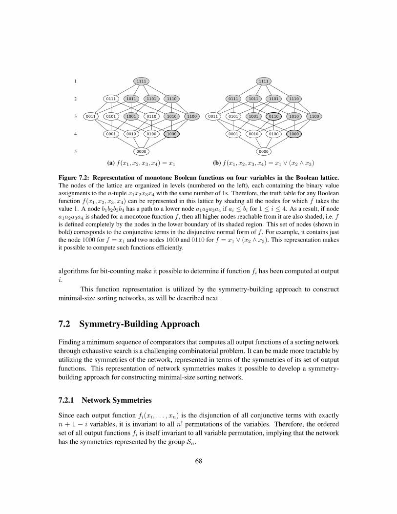
1

2

3

4

5 0000

0001 0010

0011

0100

0101 0110

0111

1000

1001 1010

1011

1100

1101 1110

1111

(a) f(x1, x2, x3, x4) = x1

0000

0001 0010

0011

0100

0101 0110

0111

1000

1001 1010

1011

1100

1101 1110

1111

(b) f(x1, x2, x3, x4) = x1 ∨ (x2 ∧ x3)

Figure 7.2: Representation of monotone Boolean functions on four variables in the Boolean lattice.The nodes of the lattice are organized in levels (numbered on the left), each containing the binary valueassignments to the n-tuple x1x2x3x4 with the same number of 1s. Therefore, the truth table for any Booleanfunction f(x1, x2, x3, x4) can be represented in this lattice by shading all the nodes for which f takes thevalue 1. A node b1b2b3b4 has a path to a lower node a1a2a3a4 if ai ≤ bi for 1 ≤ i ≤ 4. As a result, if nodea1a2a3a4 is shaded for a monotone function f , then all higher nodes reachable from it are also shaded, i.e. fis defined completely by the nodes in the lower boundary of its shaded region. This set of nodes (shown inbold) corresponds to the conjunctive terms in the disjunctive normal form of f . For example, it contains justthe node 1000 for f = x1 and two nodes 1000 and 0110 for f = x1 ∨ (x2 ∧ x3). This representation makesit possible to compute such functions efficiently.

algorithms for bit-counting make it possible to determine if function fi has been computed at outputi.

This function representation is utilized by the symmetry-building approach to constructminimal-size sorting networks, as will be described next.

7.2 Symmetry-Building Approach

Finding a minimum sequence of comparators that computes all output functions of a sorting networkthrough exhaustive search is a challenging combinatorial problem. It can be made more tractable byutilizing the symmetries of the network, represented in terms of the symmetries of its set of outputfunctions. This representation of network symmetries makes it possible to develop a symmetry-building approach for constructing minimal-size sorting network.

7.2.1 Network Symmetries

Since each output function fi(xi, . . . , xn) is the disjunction of all conjunctive terms with exactlyn + 1 − i variables, it is invariant to all n! permutations of the variables. Therefore, the orderedset of all output functions fi is itself invariant to all variable permutation, implying that the networkhas the symmetries represented by the group Sn.

68

The network also has symmetries resulting from swapping the outputs of all its comparatorsto produce its dual network with the same set of output functions in the reverse order. Doing soswaps the conjunctions and disjunctions in the output functions of the primal network to producethe output functions of the dual network. Using the symbols ∧ and ∨ to specify conjunctions anddisjunctions, this duality can be expressed as fi(xi, . . . , xn,∧,∨) = fn+1−i(xi, . . . , xn,∨,∧) forall 1 ≤ i ≤ n. It is therefore possible to define symmetry operations σi for 1 ≤ i ≤

⌈n2

⌉that act

on the network, swapping the dual functions fi and fn+1−i and also swapping the conjunctions anddisjunctions in them. Applying these operations on the ordered set of output functions leaves theset invariant. Their compositions are also symmetries because σi and σj operate independently ondifferent pairs of functions, leaving the set of outputs invariant. Therefore, this set of operationsare closed under composition and they are associative. Moreover, each operation is its own inverse,producing the identity when applied twice in a row. Thus they satisfy all the group axioms and theytherefore produce a group. Since every element of this group can be expressed as the compositionof finitely many elements of the set Σ = {σ1, . . . , σdn

2 e}, the group is said to be generated by Σand it is denoted 〈Σ〉.

The full symmetry group of the network is the combined group of symmetries resultingfrom permuting the input variables and swapping the conjunctions and disjunctions in dual outputfunctions. This group is obtained by taking the direct product of Sn and 〈Σ〉, denoted Sn × 〈Σ〉. Itsset of elements is the Cartesian product of its component groups, i.e. the set of ordered pairs (g, ρ),where g ∈ Sn and ρ ∈ 〈Σ〉. Its group operation is the component-wise composition, (g, ρ)◦(h, τ) =(g ◦ h, ρ ◦ τ). Moreover, two of its subgroups {(g, e) : g ∈ Sn} and {(e, ρ) : ρ ∈ 〈Σ〉}, wheree is the identity, are isomorphic to Sn and 〈Σ〉 respectively, confirming that Sn × 〈Σ〉 contains itscomponent groups.

Therefore, the final symmetry group of the sorting network to be designed is already known,unlike the multilegged robot controllers in Chapter 5 that required the appropriate symmetries to bediscovered by symmetry breaking. That is, any n-input sorting network has the symmetry groupSn × 〈Σ〉. Such a network can be constructed step by step through a sequence of subgoals corre-sponding to the subgroups of this symmetry group, as described next.

7.2.2 Defining Subgoal Sequence

The subgroups of Sn×〈Σ〉 represent the symmetries of partial networks created in the intermediatestages of constructing a sorting network. In particular, computing pairs of dual output functionsproduces symmetries corresponding to a subgroup of 〈Σ〉 (Figure 7.3). Since the elements of Σoperate on different pairs of dual functions, any such subgroup can be written as 〈Γ〉, where Γ is asubset of Σ. Initially, before any comparators have been added, each line i in the network has thetrivial monotone Boolean function xi. As a result, the network does not have any symmetries, i.e.Γ = {}. Adding comparators to compute both the output function fi and its dual fn+1−i yieldsΓ = {σi} for the resulting partial network. Adding more comparators to compute both fj andits dual fn+1−j creates a new partial network with Γ = {σi, σj}, i.e. the new partial network ismore symmetric. Continuing to add comparators until all output functions have been constructedproduces a complete sorting network with Γ = Σ.

69

Figure 7.3: Symmetries of output function duals in 4-input sorting networks. The number below eachcomparator indicates the sequence in which it is added to construct the network. The last comparator touchinghorizontal line i completes computing the output function fi for that line. Functions fi and fn+1−i form adual, and computing them both gives the network the symmetry σi. In network (a), comparator 3 completescomputing f1 and when comparator 4 completes computing its dual f4, the network gets the symmetry σ1.Comparator 5 then completes computing both f2 and its dual f3, giving the network another symmetry σ2.Network (b) also produces the same sequence of symmetries and has the same number of comparators. Innetwork (c), comparator 5 completes computing both f3 and f4. However, it gets the symmetries σ1 andσ2 only when comparator 6 completes computing their duals f1 and f2. Network (d) is similar, and theyboth require one more comparator than networks (a) and (b). Thus the goal set of symmetries for a 4-inputnetwork is Γ = {σ1, σ2}, i.e. it is already known. Building this set of symmetries step by step corresponds toconstructing such a network by adding comparators, some symmetry sequences requiring longer comparatorsequences. Therefore, constructing the network in this manner through a suitable sequence of symmetriescan be utilized to minimize its comparator requirement.

70

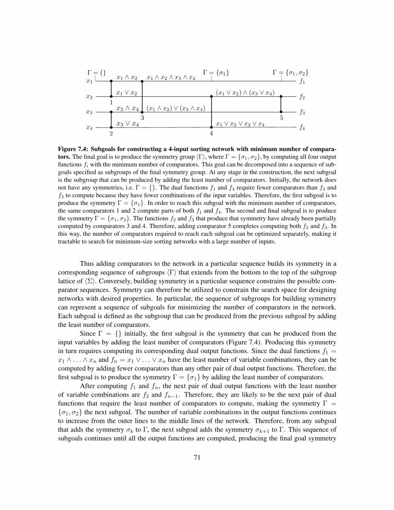
Figure 7.4: Subgoals for constructing a 4-input sorting network with minimum number of compara-tors. The final goal is to produce the symmetry group 〈Γ〉, where Γ = {σ1, σ2}, by computing all four outputfunctions fi with the minimum number of comparators. This goal can be decomposed into a sequence of sub-goals specified as subgroups of the final symmetry group. At any stage in the construction, the next subgoalis the subgroup that can be produced by adding the least number of comparators. Initially, the network doesnot have any symmetries, i.e. Γ = {}. The dual functions f1 and f4 require fewer comparators than f2 andf3 to compute because they have fewer combinations of the input variables. Therefore, the first subgoal is toproduce the symmetry Γ = {σ1}. In order to reach this subgoal with the minimum number of comparators,the same comparators 1 and 2 compute parts of both f1 and f4. The second and final subgoal is to producethe symmetry Γ = {σ1, σ2}. The functions f2 and f3 that produce that symmetry have already been partiallycomputed by comparators 3 and 4. Therefore, adding comparator 5 completes computing both f2 and f3. Inthis way, the number of comparators required to reach each subgoal can be optimized separately, making ittractable to search for minimum-size sorting networks with a large number of inputs.

Thus adding comparators to the network in a particular sequence builds its symmetry in acorresponding sequence of subgroups 〈Γ〉 that extends from the bottom to the top of the subgrouplattice of 〈Σ〉. Conversely, building symmetry in a particular sequence constrains the possible com-parator sequences. Symmetry can therefore be utilized to constrain the search space for designingnetworks with desired properties. In particular, the sequence of subgroups for building symmetrycan represent a sequence of subgoals for minimizing the number of comparators in the network.Each subgoal is defined as the subgroup that can be produced from the previous subgoal by addingthe least number of comparators.

Since Γ = {} initially, the first subgoal is the symmetry that can be produced from theinput variables by adding the least number of comparators (Figure 7.4). Producing this symmetryin turn requires computing its corresponding dual output functions. Since the dual functions f1 =x1 ∧ . . . ∧ xn and fn = x1 ∨ . . . ∨ xn have the least number of variable combinations, they can becomputed by adding fewer comparators than any other pair of dual output functions. Therefore, thefirst subgoal is to produce the symmetry Γ = {σ1} by adding the least number of comparators.

After computing f1 and fn, the next pair of dual output functions with the least numberof variable combinations are f2 and fn−1. Therefore, they are likely to be the next pair of dualfunctions that require the least number of comparators to compute, making the symmetry Γ ={σ1, σ2} the next subgoal. The number of variable combinations in the output functions continuesto increase from the outer lines to the middle lines of the network. Therefore, from any subgoalthat adds the symmetry σk to Γ, the next subgoal adds the symmetry σk+1 to Γ. This sequence ofsubgoals continues until all the output functions are computed, producing the final goal symmetry

71

Γ = {σ1, . . . , σdn2 e}. The number of comparators required to reach each of these subgoals is

minimized as described next.

7.2.3 Minimizing Comparator Requirement

In order to reach the first subgoal, the same comparator can compute a conjunction for f1 andalso a disjunction for fn simultaneously (Figure 7.4). Sharing the same comparator to compute dualfunctions in this manner reduces the number of comparators required in the network. However, suchsharing between dual functions of the same subgoal is possible only in some cases. In other cases,it may still be possible to share a comparator with the dual function of a later subgoal. Constructingminimal-size sorting networks requires determining which comparators can be shared and thenadding those comparators that maximize sharing.

The Boolean lattice representation of functions discussed in Section 7.1 can be utilized todetermine whether sharing a comparator by computing parts of two functions simultaneously ispossible (Figure 7.5). Assume that the current subgoal requires computing the output function fi

and its dual fn+1−i. That is, functions for outputs less than i and greater than n+1− i have alreadybeen computed. All the remaining output functions will need to have the value 1 for all nodes inlevels less than or equal to i and the value 0 for all nodes in levels greater than n+ 1− i. Therefore,the current functions on lines i ≤ j ≤ n + 1 − i are also guaranteed to have the same values forthose levels. Otherwise, computing at least one of the output functions by adding comparators willbe impossible (since conjunctions preserve 0s and disjunctions preserve 1s).

For the current subgoal, function fi can be computed by setting its value for all nodes in leveli to 1 and all nodes in level i+1 to 0, thus defining its node boundary in the lattice. Its monotonicitythen implies that its value for all nodes in levels less than i will be set to 1 automatically and itsvalue at all nodes in levels greater than i + 1 will be set to 0 automatically. However, since fi iscomputed from the current functions f ′j on lines i ≤ j ≤ n+ 1− i and they already have the value1 for all nodes in levels less than or equal to i, the function fi will also get the same value for thosenodes automatically. Therefore, fi can be computed just by setting the values for all nodes in leveli+ 1 to 0.

The value for a particular node is set to 0 by utilizing a comparator that computes its con-junction with another function that already has the value 0 for that node. Moreover, the disjunctionthat the comparator also computes has the value 1 for all nodes in level i + 1 as required for theother output functions that are yet to be computed. Therefore, exactly one of the functions f ′j al-ready has the value 0 for any particular node in level i+ 1. Adding a comparator between a pair ofsuch functions computes their conjunction with the 0-valued nodes from both functions. Repeatingthis process recursively collects the 0-valued nodes in level i+ 1 from all functions to the functionon line i, thus producing fi. Similarly, its dual function fn+1−i can also be computed from thefunctions f ′j by utilizing disjunctions instead of conjunctions to set its values for all nodes in leveln+ 1− i to 1.

The leaves of the resulting binary recursion tree for fi are the functions f ′j that have 0-valued nodes in level i+ 1 and its internal nodes are the comparators. Since the number of nodes ofdegree 2 in a binary tree is one less than the number of leaves (Mehta and Sahni, 2005), the number

72

1

2

3

4

5 0000

0001 0010

0011

0100

0101 0110

0111

1000

1001 1010

1011

1100

1101 1110

1111

(a) x1

0000

0001 0010

0011

0100

0101 0110

0111

1000

1001 1010

1011

1100

1101 1110

1111

(b) x2

1

2

3

4

5 0000

0001 0010

0011

0100

0101 0110

0111

1000

1001 1010

1011

1100

1101 1110

1111

(c) x1 ∧ x2

0000

0001 0010

0011

0100

0101 0110

0111

1000

1001 1010

1011

1100

1101 1110

1111

(d) x1 ∨ x2

Figure 7.5: Comparator sharing to compute dual output functions in a 4-input sorting network. Thisfigure illustrates the Boolean lattice representation of the functions computed by comparator 1 in Figure 7.4.The levels of the lattices are numbered on the left and the nodes for which the function value is 1 are shaded.Comparator 1 computes the conjunction (c) and the disjunction (d) of the functions (a) and (b) for the subgoalof computing the output functions f1 = x1 ∧ x2 ∧ x3 ∧ x4 and f4 = x1 ∨ x2 ∨ x3 ∨ x4. Function f1 can becomputed by utilizing conjunctions to set the value for all nodes in level 2 of the lattice to 0. Similarly, f4 canbe computed by utilizing disjunctions to set the value for all nodes in level 4 to 1. Therefore, comparator 1contributes to computing both f1 and f4 by setting the values of two nodes in level 2 of its conjunction to 0and the values of two nodes in level 4 of its disjunction to 1. Such shared computation reduces the number ofcomparators required to construct sorting networks.

of comparators required depends only on the number of functions the recursion starts with, i.e. it isinvariant to the order in which the recursion pairs the leaves. However, the recursion trees for fi andfn+1−i may have common leaves, making it possible to utilize the same comparator to compute aconjunction for fi and a disjunction for fn+1−i. Maximizing such sharing of comparators betweenthe two recursion trees minimizes the number of comparators required for the current subgoal.

It may also be possible to share a comparator with a later subgoal, e.g. when it computes aconjunction for fi and a disjunction for fn+1−k, where i < k ≤

⌈n2

⌉. In order to prioritize subgoals

and determine which comparators maximize sharing, each pair of lines where a comparator canpotentially be added is assigned a utility. Comparators that contribute to both fi and fn+1−i for

73

the current subgoal get the highest utility. Comparators that contribute to an output function for thecurrent subgoal and an output function for the next subgoal get the next highest utility. Similarly,other possible comparators are also assigned utilities based on the output functions to which theycontribute and the subgoals to which those output functions belong. Many comparators may havethe same highest utility; therefore, one comparator is chosen randomly from that set and it is addedto the network. Repeating this process produces a sequence of comparators that optimizes sharingwithin the current subgoal and between the current subgoal and later subgoals.

7.3 Evolving Minimal-Size Networks

Optimizing for each subgoal separately in the above manner constitutes a greedy algorithm thatproduces minimal-size networks with high probability for n ≤ 8. However, for larger values of n,the number of subgoals is too many to find a global optimum reliably. In such cases, its performancecan be improved by utilizing evolution to optimize the solutions further.

The most straightforward approach is to initialize evolution with a population of solutionsthat the greedy algorithm produces. The fitness of each solution is the negative of its number ofcomparators so that improving fitness will minimize the number of comparators. In each genera-tion, two-way tournament selection based on this fitness measure is utilized to select the best indi-viduals in the population for reproduction. Reproduction mutates the parent network, creating anoffspring network in two steps: (1) a comparator is chosen from the network randomly to truncatethe network, discarding all comparators that were added after it, and (2) the greedy algorithm is uti-lized to add comparators again, reconstructing a new offspring network. Since the greedy algorithmchooses a comparator with the highest utility randomly, this mutation explores a new combinationof comparators that might be more optimal than the parent.

This straightforward approach restricts the search to the space of comparator combinationssuggested by the greedy algorithm and assumes that it contains a globally minimal network. Butin some cases, the globally minimal networks may utilize comparators that are different from thosesuggested by the greedy algorithm. Therefore, a more powerful (but still brute force) approach isto let evolution utilize such comparators as well: With a low probability, the suggestions of thegreedy algorithm are ignored and instead the next comparator to be added to the network is selectedrandomly from the set of all potential comparators.

A more effective way to combine evolution with such departures from the greedy algorithmis to utilize an Estimation of Distribution Algorithm (EDA) (Alden, 2007, Bengoetxea et al., 2001,Muhlenbein and Hons, 2005). The idea is to estimate the probability distribution of optimal com-parator combinations and to utilize this distribution to generate comparator suggestions. The EDA isinitialized as before with a population of networks generated by the greedy algorithm. In each gen-eration, a set of networks with the highest fitness are selected from the population. These networksare utilized in three ways: (1) to estimate the distribution of optimal comparators for a generativemodel, (2) as elite networks passed unmodified to the next generation, and (3) as parent networksfrom which new offspring networks are created for the next generation.

The generative model of the EDA specifies the probability P (C|S) of adding a comparatorC to an n-input partial network with state S. The state of a partial network is defined in terms of

74

0000

0001 0010

0011

0100

0101 0110

0111

1000

1001 1010

1011

1100

1101 1110

1111 01

00

00

10

10

Figure 7.6: State representation of the function x1 ∧ x2 utilized in the EDA. The state (shown on theright) is a bit-string with two bits for each level of the Boolean lattice. The first bit is 1 only if the value of thefunction for all nodes in that level is 0 and the second bit is 1 only if its value for all nodes in that level is 1.This condensed representation of the function is based on the information utilized by the symmetry-buildinggreedy algorithm and it is therefore useful for constructing minimal-size sorting networks.

the n Boolean functions that its comparators compute. These functions determine the remainingcomparators that are needed to finish computing the output functions, making them a good repre-sentation of the partial network. However, storing the state as the concatenation of the n functionsis computationally intractable since each function is represented as a vector of 2n bits. Therefore, acondensed state representation is computed based on the observation that the greedy algorithm doesnot utilize the actual function values for the nodes in the Boolean lattice; it only checks whether thevalues in a given level are all 0s or all 1s. This information, encoded as 2(n + 1) bits (Figure 7.6),is suitable as the state representation for the model as well.

Since the model is estimated from the set of the smallest networks in the population, it islikely to generate small networks as well. Although it can generate new networks from scratch,it is utilized as part of the above reproduction mechanism to reconstruct a new offspring networkfrom the truncated parent network, i.e. it is utilized in step 2 of reproduction instead of the greedyalgorithm. In this step, some comparators are also chosen randomly from the set of all potentialcomparators to encourage exploration of comparator combinations outside the model. Moreover,if the model does not generate any comparators for the current state, then the greedy algorithmis utilized to add a comparator. The resulting EDA finds smaller sorting networks than previousresults, as demonstrated next.

7.4 Results

The EDA was run with a population size of 200 for 500 generations to evolve minimal-size networksfor different input sizes. In each generation, the top half of the population (i.e. 100 networks withthe least number of comparators) was selected for estimating the model. The same set of networkswas copied to the next generation without modification. Each of them also reproduced an offspringnetwork to replace those in the bottom half of the population. A Gaussian probability distributionwas utilized to select the comparator from which to truncate the parent network. The Gaussian

75

n 12 13 14 15 16 17 18 19 20 21 22 23 24

Previous bestHand-design and END Batcher’s merge on smaller networks39 45 51 56 60 73 80 88 93 103 110 118 123

EDA 39 45 51 57 60 71 78 86 92 103 108 118 125

Table 7.1: Sizes of the smallest networks for different input sizes found by the EDA. For input sizesn ≤ 11, networks with the smallest-known sizes (Section 3.3) were already found in the initial population ofthe EDA, i.e. the greedy algorithm was sufficient. These sizes are therefore omitted from this table. For largerinput sizes, evolution found networks that matched previous best results (indicated in italics) or improvedthem (indicated in bold). Appendix A lists examples of these networks. EDA variant 2 produced betterresults than variant 1 for input sizes 15, 17, 18, 20, 22, 23, and 24. Prospects of extending these results toinput sizes greater than 24 will be discussed in Chapter 8. These results demonstrate that the symmetry-basedEDA approach is effective at designing minimal-size sorting networks and has advanced the state-of-the-art.

was centered at the middle of its comparator sequence with a standard deviation of one-fourth itsnumber of comparators. As a result, parent networks are more likely to be truncated near the middlethan near the ends. When reconstructing the truncated network, the next comparator to add to thenetwork is generated either by the estimated model (with probability 0.5) or is selected randomlyfrom the set of all potential comparators (with probability 0.5).

The above experiments (variant 1) were repeated with a slight modification of the greedyalgorithm used to initialize the population for the EDA. If the set of comparators with the highestutility contains a comparator that is symmetric with respect to another comparator already in thenetwork, then it prefers that comparator (Graham and Oppacher, 2006). This modification (vari-ant 2) makes the arrangement of comparators in the network more bilaterally symmetric about ahorizontal axis through the middle of the network. Biasing the networks with this type of symmetryproduced smaller networks for some input sizes. The source code for both variants is available fromthe website http://nn.cs.utexas.edu/?sorting-code.

Both variants were run 20 times, each time with a different random number seed. The leastnumber of comparators that they found for each input size is listed in Table 7.1. For input sizesn ≤ 11, the initial population of the EDA already contained networks with the smallest-knownsizes for all 20 runs, i.e. the greedy algorithm was sufficient to find the smallest-known networks.As discussed in Section 3.3, optimality of such networks has been proven only for n ≤ 8. Forinput sizes 12, 13, 14, 16, 21, and 23, the EDA evolved networks that have the same size as the bestknown networks. Moreover, it improved the previous best results for input sizes 17, 18, 19, 20, and22 by one or two comparators. Examples of these networks are listed in Appendix A. Prospects ofextending to n > 24 will be discussed in Chapter 8.

The previous best results were obtained either by hand design or by the END evolutionaryalgorithm (Baddar, 2009, Juille, 1995, Knuth, 1998). The END algorithm improved a 25-year oldresult for the 13-input case by one comparator and matched the best known results for other inputsizes up to 16. However, it is a massively parallel search algorithm, requiring very large computa-tional resources, e.g. it required a population size of 65,536 on 4096 processors to find minimal-sizenetworks for 13 and 16 inputs. In contrast, the symmetry-based EDA algorithm finds such networks

76

http://nn.cs.utexas.edu/?sorting-code

with much smaller resources (e.g. population size of 200 on a single processor in a similar numberof generations), making it computationally feasible to solve larger problems.

7.5 Conclusion

Minimizing the number of comparators in a sorting network is a challenging optimization problem.This chapter presented an approach that converts it into the problem of building the symmetry of thenetwork optimally. The resulting problem structure makes it possible to construct the network insteps and to minimize the number of comparators required for each step separately. This approachproduces greedy solutions that are optimized further by evolution, exploring the neighborhood ofthese solutions in more detail. As with ENSO, the resulting algorithm focuses search on promisingregions of the search space, making it possible to find minimal-size networks efficiently. For severalinput sizes, these networks are smaller than the previous best results, thus advancing the state-of-the-art for designing minimal-size sorting networks.

77

Chapter 8

Discussion and Future Work

The work presented in previous chapters explored the hypothesis that symmetry can be utilized toconstrain the design space meaningfully, making it possible to solve challenging engineering prob-lems. For multilegged robots walking on flat ground, it was possible to constrain the controllers toa single hand-designed symmetry and evolve only the remaining parameters. Since it is not alwayspossible to hand-design the appropriate symmetries, the ENSO approach was developed to evolvethem automatically. ENSO utilizes group theory to break symmetry systematically, thereby con-straining search to the most promising symmetries. The alternative process of building symmetrysystematically was also useful in constraining the search space for finding minimal-size sorting net-works. This chapter evaluates these results, discusses the insights gained from them, and proposesdirections for future work.

8.1 Hand-Designed Symmetries

Modular neuroevolution with hand-designed symmetries produced controllers that were better thanthose produced by non-modular evolution with no symmetries in two respects: (1) they achieveda better fitness by travelling farther, and (2) they employed better gaits that were symmetric, re-sembling those found in nature. Furthermore, this performance gap widened significantly in bothrespects when the number of legs or their degrees of freedom were increased. The symmetric con-trollers also demonstrated the capability to change gaits in response to changes in the environment.Changing gaits on an obstacle terrain made it easier for the robot to negotiate bumps. These re-sults suggest that utilizing symmetries to constrain the search space makes it possible for modularneuroevolution to discover effective controllers.

In these experiments, the controllers were always evaluated by starting the robot from thesame position. As a result, some evolved behaviors such as changing gaits to negotiate obstacles arenot robust to different starting positions. They can be made more robust by averaging evaluationsover multiple random starting positions or by adding noise to the simulation during evaluations aswas done for the physical robot. Utilizing sensors that provide feedback about the environment mayalso improve robustness.

78

The controller symmetries were designed analytically using the theory of coupled cell sys-tems. Hand-designing symmetries in this manner is too restrictive in the general case for two rea-sons. First, in the special case it was possible to replicate a single module for each leg because thelegs were identical. In a more complex robot, more than one type of module may be needed, forexample to control different types of front and rear legs. The resulting coupled cell system will havemore than one type of cell and therefore different symmetries. Second, in the special case the cou-pling between the cells and the assignment of cells to legs was also determined by the hand-designedsymmetries. More sophisticated behaviors may require different cell couplings and assignments thatutilize different symmetries to explore a different part of the search space. Although hand-designingsymmetries is possible in simple cases, it cannot (at least not as easily) be done in such complex,real-world cases.

Therefore, it is useful to evolve the appropriate symmetries automatically. However, theresults of non-modular evolution suggests that it is too difficult to evolve symmetries in the uncon-strained space of all possible symmetries. Consequently, a more constrained approach that makes itpossible to explore the space of symmetries in a meaningful way is necessary. The ENSO approachaccomplishes this goal.

8.2 Symmetry Evolution with ENSO

Given the number of modules, ENSO’s group-theory-based systematic symmetry search makes itpossible to evolve the appropriate symmetry automatically. Demonstrating this capability, ENSOevolved gaits similar to those based on hand-designed symmetries on flat ground, and significantlyfaster gaits on inclined ground, for a quadruped robot. These gaits also generalized better when fric-tion was reduced to make the ground slippery. As in the previous experiments with hand-designedsymmetries, these gaits were evolved by starting the robot from the same position and orientationon the incline in every evaluation. More robust gaits can potentially be evolved by randomizing theinitial orientation, by sensing the slope of the incline, or by adding noise to the simulation. Suchrobust gaits were indeed evolved for the physical robot in Chapter 6.

In order to verify that ENSO’s symmetry-breaking approach is indeed a useful way toconstrain search, it was compared with the less principled, random-symmetry-evolution approach.Random-symmetry evolution produces significantly worse gaits than ENSO because its unsystem-atic symmetry mutations often result in large changes in symmetry. In contrast, the group-theoreticmutations of ENSO result in only minimal changes in symmetry, making complexification possible(Section 2.1): Evolution starts with a highly symmetric (i.e. simple) controller and breaks the sym-metry incrementally, producing gradual increases in complexity. As a result, evolution optimizessimpler controllers before elaborating on these by adding more parameters. Thus the complexifi-cation resulting from symmetry breaking provides ENSO with a smoother fitness gradient, makingevolution easier.

In addition to these evolutionary advantages that group theory provides, the theory of cou-pled cell systems provides ENSO with guarantees on the behavior of evolved controllers. For exam-ple, if the symmetries of a coupled cell system admit a particular gait, then there exists an instanceof the system with an asymptotically stable periodic solution (i.e. limit cycle) implementing that

79

gait (Golubitsky and Stewart, 2002). As a result, the gait is robust to small perturbations. ENSOconstrains neuroevolution to find such an instance of the control system. When the dynamics ofthis system was perturbed manually (utilizing a visualization interface to the physical simulation)the gaits they generate were indeed found to be robust. Such robustness is useful in controllers ofreal-world robots because their interactions with environment are frequently perturbed.

As discussed in Section 2.3, the symmetries of coupled cell systems also makes it possiblefor the same controller to produce multiple gaits. Each gait is a stable limit cycle of the coupled cellsystem, and the system can transition from one limit cycle to another when perturbed. Sometimessmall perturbations, caused by physical interaction with the environment, can trigger such a transi-tion. Figure 5.5d shows an example of this phenomenon, where the robot changes from an initialpronk to a trot at about three seconds into the simulation. If the robot is prevented from interactingwith the ground, then this change does not occur and the robot continues executing the pronk gait.The ability of controllers to generate such different gaits makes it possible to use the most effectivegait for a given terrain, including those that allow it to go over obstacles (Section 4.7).

It is difficult to obtain the above properties in controllers evolved without such mathematicalmodels. For example, oscillations required for generating gaits needed to be supplied as externalinputs to quadruped controllers evolved using the HyperNEAT method (Clune et al., 2009). Theseproperties were crucial in transferring the controllers that ENSO evolved in simulation to a physicalrobot.

These results suggest that ENSO is an effective approach for evolving locomotion con-trollers for multilegged robots. In the future, ENSO should be tested with more complex robotswith more legs, more complex legs, and sensors that receive more varied stimuli from the environ-ment. Their controllers can be modeled as coupled cell systems with more cells and cells receivingadditional inputs. Utilizing such more sophisticated models should make it possible for ENSO toevolve controllers that produce high-level behaviors such as path-following and foraging, in addi-tion to generating regular gaits. ENSO is thus a promising approach for developing efficient, robust,and flexible controllers for multilegged robots in the real world.

ENSO breaks symmetry by utilizing the prior knowledge encoded in the subgroup lattice.In contrast, symmetry-breaking occurs spontaneously in nature when perturbations induce a phys-ical system in a symmetric (but unstable) state to transition to a less symmetric (but stable) statewith lower energy (Brading and Castellani, 2008, Kovacs, 1986). That is, the dynamics of naturalphenomena encode the knowledge in the subgroup lattice implicitly. Nature can therefore utilizethese phenomena to break symmetry in biological evolution. Whether modeling them in artificialevolution is an effective substitute for the constraints encoded explicitly in the subgroup lattice is aninteresting question for future research.

8.3 Evolving Controllers for a Physical Robot

ENSO evolved controllers that produced the same gaits in the physical robot as they did in simula-tion. Moreover, these gaits were robust to uncertainties that commonly occur in the real world suchas changes in ground friction between different surfaces, initial positions of legs from which therobot starts walking, and the maximum angular velocity that the motors can produce. The transfer

80

was successful because of two factors: (1) ENSO was able to evolve robust controllers that pro-duce stable gaits, and (2) it was possible to simulate the physical characteristics of the robot withsufficient accuracy.

It is often difficult to transfer controllers evolved in simulation to the real world because itis difficult to simulate the physical robot and its environment accurately (Gomez and Miikkulainen,2004, Lipson et al., 2006). However, this requirement is less critical for the controllers that ENSOevolves because their robustness can compensate for small deviations from ideal behavior. Forexample, instead of detailed mesh models of the robot morphology, only a crude approximation ofits weight distribution was required. Moreover, it turned out sufficient to model the idiosyncraticproperties of the motors and uncertainties in their behavior using interpolation and noise.

Evolving controllers in simulation and then transferring them to the real robot in this man-ner is an effective alternative to designing controllers by hand. Hand-design is difficult because itrequires anticipating all possible operating conditions. Moreover, this laborious process has to berepeated whenever the configuration of the robot changes and it may even be impossible in somecases. In contrast, evolution can design a new controller automatically for the new configurationin simulation. For example, if a leg actuator fails on a quadruped robot during a remote mission,then it must continue the mission with minimum performance degradation by utilizing only the re-maining three legs. ENSO evolved a straight and effective gait for such a three-legged configurationby disabling a leg in simulation. The resulting controller produced the same gait when transferredto the physical robot as well, suggesting that ENSO’s symmetry-based approach can be utilized todesign fault-tolerant robots for real-world applications.

The physical quadruped robot can be extended to a hexapod easily by adding two morelegs to attachments in the middle. This extension should be able to demonstrate that the ENSOapproach scales up for a physical robot with more legs. ENSO can also be tested on a robot withmore complex legs by designing new legs with additional joints. Another interesting way to extendthe robot is to attach Dynamixel AX-S1 sensors to measure distance Robotis (2010). Readingsfrom these sensors can then be used as additional controller inputs, making it possible to evolvebehaviors that respond effectively to obstacles in the environment. Such extensions can build up thesophistication necessary for real-world applications.

8.4 Utilizing Domain Knowledge in ENSO

ENSO can also evolve controllers for robots with more legs and more degrees of freedom per leg,such as those discussed in Chapter 4. These robots may have more joints per leg such as a kneejoint in addition to the hip joint. The controllers for such robots may need a different module foreach type of joint. Moreover, the knee joint of one leg is not likely to influence the hip joint ofanother leg directly, allowing this domain knowledge to be used to restrict the connectivity of thegraphs in the initial population of ENSO. In particular, each knee module is connected only to thehip module of the same leg, while the hip modules of all legs are fully interconnected as before.Utilizing domain knowledge in this manner to constrain the space of symmetries makes it easier forevolution to optimize the resulting controller.

81

PhenotypeGenotype

5 6

7

5 6

7

5 6

7

5 6

7

1 2

3 4

V x V:Params:

1111111111111111

p1,...,pk q1...,qm

Nil


V x V:Params:

111111111

p1,...,pk q1...,qm

Nil


Figure 8.1: A two-level hierarchical genotype and phenotype. Modules of the top-level of the phenotypegraph are decomposed into smaller interconnected modules, creating the bottom-level phenotype graphs. Inthe top-level of the corresponding genotype tree, the vertex color contains a special parameter that stores thegenotype tree for the bottom-level phenotype graph. Decomposing the phenotype graph into smaller graphsin this manner should make it easier to evolve its symmetry, and constitutes an interesting direction of futurework.

The above robot morphology can be extended further by adding a foot joint to each leg, re-sulting in a controller with local interconnections between the hip, knee and foot modules. However,it is more convenient to represent such controllers using a two-level hierarchy instead of using a flatstructure. The top level of the hierarchy contains the interconnection structure between leg modules.Each leg module is then decomposed into a second level, containing the interconnection structurebetween the hip, knee and foot modules for that leg. Such a hierarchical phenotype graph can beencoded by a hierarchical genotype tree (Figure 8.1). The vertex color in the top-level tree containsa special parameter that is a pointer to the bottom-level genotype tree. This hierarchical genotypeallows the phenotype structure of each level to evolve independently. Moreover, it decomposes thephenotype graph into smaller graphs, whose symmetries can be evolved more easily because theirautomorphism groups are smaller.

Future experiments along these lines should demonstrate that (1) domain knowledge can beeffectively incorporated into the ENSO approach by constraining the initial structure of the phe-notype graph, and (2) the ENSO approach can design complex controller networks consisting ofdifferent modules and interconnection structures by evolving them together. These capabilities maybe necessary to design controllers for complex robots, e.g. amphibious robots that can swim in waterand walk on land, robotic manipulators that consist of several parts for use in industrial applications,and serpentine robots that move by flexing their spine.

82

8.5 Other Applications of ENSO

ENSO can also be used to evolve solutions for other control problems that are characterized by sym-metry and modularity. For example, it can be used to design multiagent systems consisting of agentsthat interact with each other and with the environment, like those in online auctions and in roboticsoccer (Stone and Veloso, 2000). The behavior of these agents can be represented as neural networkmodules and their interactions as (symmetric) connections between the modules. Another applica-tion is in designing distributed control systems for automated manufacturing processes (McFarlane,1998). Such systems consist of controller modules interconnected by communication networksand they can therefore be implemented as modular neural networks. In both cases, identical mod-ules and connections between them produce symmetries that ENSO can evolve to design effectivecontrol systems. Similarly, ENSO can be used to design distributed computing systems such as acomputer network of clients and servers by evolving the parameters and topology of those networks(Berryman et al., 2004).

Besides controllers for multilegged locomotion, coupled cell systems can also model otherdynamical systems in nature as symmetric networks. As a result, ENSO can potentially be used tooptimize them. For example, coupled cell systems have been used to study the formation of newspecies in nature (Golubitsky and Stewart, 2002), the role of structural symmetries of the visualcortex in inducing visual hallucinations (Golubitsky et al., 2003), and the properties of geneticregulatory networks (Edwards and Glass, 2000). ENSO can be used as a tool both for understandingsuch biological phenomena and for engineering artificial systems based on them.

8.6 Extending ENSO

Some of the above applications may require extending ENSO in various ways to improve its capabil-ities. First, modules with a fixed neural network architecture (i.e. network topology) was sufficientfor the multilegged robot controllers that ENSO evolved in this dissertation. However, more com-plex applications may require more complex topologies. In such applications, ENSO can evolve thetopology of the modules by utilizing techniques such as NEAT (Stanley and Miikkulainen, 2004).

Second, in many applications such as distributed controllers and multiagent systems, thenumber of modules remains fixed and is known. ENSO requires the user to specify this domainknowledge, making it possible to initialize evolution with the appropriate most general symmetries.However, in other applications such as biological networks (Kepes, 2007) and body-brain evolution(Bongard and Pfeifer, 2003), the modules may not be known a priori. If the number of modulesis constant as in biological networks, then ENSO can potentially be extended with clustering algo-rithms to determine the modules automatically (Gao et al., 2009). If the number of modules changesas in body-brain evolution, then ENSO will have to change the subgroup lattice accordingly.

Third, crossover of genotypes to produce offspring is useful in applications that benefitfrom the building-block hypothesis: In such applications, it is possible to assemble functionallycomplementary blocks from different parents (Watson and Jansen, 2007). Therefore, in addition tothe mutation operators that ENSO already implements, it should be extended to include crossover,e.g. by swapping subtrees that have the same structure and node colors. Such subtrees preserve

83

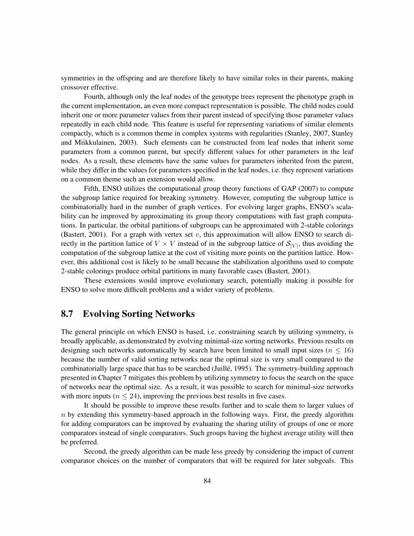
symmetries in the offspring and are therefore likely to have similar roles in their parents, makingcrossover effective.

Fourth, although only the leaf nodes of the genotype trees represent the phenotype graph inthe current implementation, an even more compact representation is possible. The child nodes couldinherit one or more parameter values from their parent instead of specifying those parameter valuesrepeatedly in each child node. This feature is useful for representing variations of similar elementscompactly, which is a common theme in complex systems with regularities (Stanley, 2007, Stanleyand Miikkulainen, 2003). Such elements can be constructed from leaf nodes that inherit someparameters from a common parent, but specify different values for other parameters in the leafnodes. As a result, these elements have the same values for parameters inherited from the parent,while they differ in the values for parameters specified in the leaf nodes, i.e. they represent variationson a common theme such an extension would allow.

Fifth, ENSO utilizes the computational group theory functions of GAP (2007) to computethe subgroup lattice required for breaking symmetry. However, computing the subgroup lattice iscombinatorially hard in the number of graph vertices. For evolving larger graphs, ENSO’s scala-bility can be improved by approximating its group theory computations with fast graph computa-tions. In particular, the orbital partitions of subgroups can be approximated with 2-stable colorings(Bastert, 2001). For a graph with vertex set v, this approximation will allow ENSO to search di-rectly in the partition lattice of V × V instead of in the subgroup lattice of S|V |, thus avoiding thecomputation of the subgroup lattice at the cost of visiting more points on the partition lattice. How-ever, this additional cost is likely to be small because the stabilization algorithms used to compute2-stable colorings produce orbital partitions in many favorable cases (Bastert, 2001).

These extensions would improve evolutionary search, potentially making it possible forENSO to solve more difficult problems and a wider variety of problems.

8.7 Evolving Sorting Networks

The general principle on which ENSO is based, i.e. constraining search by utilizing symmetry, isbroadly applicable, as demonstrated by evolving minimal-size sorting networks. Previous results ondesigning such networks automatically by search have been limited to small input sizes (n ≤ 16)because the number of valid sorting networks near the optimal size is very small compared to thecombinatorially large space that has to be searched (Juille, 1995). The symmetry-building approachpresented in Chapter 7 mitigates this problem by utilizing symmetry to focus the search on the spaceof networks near the optimal size. As a result, it was possible to search for minimal-size networkswith more inputs (n ≤ 24), improving the previous best results in five cases.

It should be possible to improve these results further and to scale them to larger values ofn by extending this symmetry-based approach in the following ways. First, the greedy algorithmfor adding comparators can be improved by evaluating the sharing utility of groups of one or morecomparators instead of single comparators. Such groups having the highest average utility will thenbe preferred.

Second, the greedy algorithm can be made less greedy by considering the impact of currentcomparator choices on the number of comparators that will be required for later subgoals. This

84

analysis will make it possible to optimize across subgoals, potentially producing smaller networksat the cost of additional computations.

Third, the state representation that the EDA algorithm utilizes contains only sparse infor-mation about the functions computed by the comparators. Extending it to include more relevantinformation should make it possible for the EDA to disambiguate overlapping states and thereforeto model comparator distribution more accurately.

Fourth, the EDA generates comparators to add to the network only if the state of the networkmatches a state in the generative model exactly. Making this match fuzzy based on some similaritymeasure may produce better results by exploring similar states when an exact match is not found.

Fifth, evolutionary search can be parallelized, e.g. using the massively parallel END al-gorithm that has been shown to evolve the best known network sizes for n ≤ 16 (Juille, 1995).Utilizing the symmetry-building approach to constrain the search space should make it possible torun the END algorithm on networks with more inputs.

Sixth, the symmetry-building approach itself can be improved. For example, it utilizes onlythe symmetries resulting from the duality of the output functions. It may be possible to extend thisapproach by also utilizing the symmetries resulting from the permutations of the input variables.

Seventh, large networks can be constructed from smaller networks by merging the outputsof the smaller networks. Since smaller networks are easier to optimize, they can be evolved firstand then merged by continuing evolution to add more comparators. This construction is similarto utilizing the odd-even merge (Batcher, 1968) to construct minimal networks for n > 16 fromsmaller networks.

In addition to finding minimal-size networks, the same symmetry-based approach can alsobe utilized to find minimal-delay networks. Instead of minimizing the number of comparators, itwould now minimize the number of parallel steps into which the comparators are grouped. Boththese objectives can be optimized simultaneously as well, either by preferring one objective overthe other in the fitness function or by utilizing a multi-objective optimization algorithm such asNSGA-II (Deb et al., 2000).

Moreover, this approach can potentially be extended to design comparator networks forother related problems such as rank order filters (Chakrabarti and Wang, 1994, Chung and Lin,1997, Hiasat and Hasan, 2003). A rank order filter with rank r selects the rth largest element froman input set of n elements. Such filters are widely used in image and signal processing applications,e.g. to reduce high-frequency noise while preserving edge information. Since these filters are oftenimplemented in hardware, minimizing their comparator requirement is necessary to minimize theirchip area. More generally, similar symmetry-based approaches may be useful for designing stackfilters, i.e. circuits implementing monotone Boolean functions, which are also popular in signalprocessing applications (Hiasat and Hasan, 2003, Shmulevich et al., 1995). Furthermore, suchapproaches can potentially be used to design rearrangeable networks for switching applications aswell (Seo et al., 1993, Yeh and Feng, 1992).

85

8.8 Conclusion

Utilizing symmetries to constrain evolutionary search improves search efficiency in problems asvaried as designing controllers for multilegged robots and constructing minimal-size sorting net-works. Depending on the nature of the problem, these constraints are applied either by breakingsymmetries as in controller design or by building symmetries as in sorting network optimization.As discussed in this chapter, these methods may also benefit a variety of other problems with sym-metries. Also, several proposed extensions should make it possible to solve even harder instancesof these problems.

86

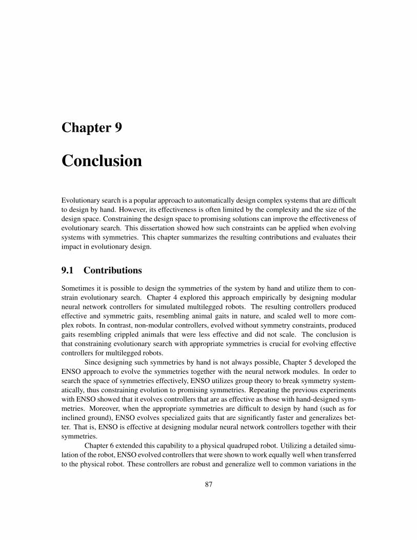
Chapter 9

Conclusion

Evolutionary search is a popular approach to automatically design complex systems that are difficultto design by hand. However, its effectiveness is often limited by the complexity and the size of thedesign space. Constraining the design space to promising solutions can improve the effectiveness ofevolutionary search. This dissertation showed how such constraints can be applied when evolvingsystems with symmetries. This chapter summarizes the resulting contributions and evaluates theirimpact in evolutionary design.

9.1 Contributions

Sometimes it is possible to design the symmetries of the system by hand and utilize them to con-strain evolutionary search. Chapter 4 explored this approach empirically by designing modularneural network controllers for simulated multilegged robots. The resulting controllers producedeffective and symmetric gaits, resembling animal gaits in nature, and scaled well to more com-plex robots. In contrast, non-modular controllers, evolved without symmetry constraints, producedgaits resembling crippled animals that were less effective and did not scale. The conclusion isthat constraining evolutionary search with appropriate symmetries is crucial for evolving effectivecontrollers for multilegged robots.

Since designing such symmetries by hand is not always possible, Chapter 5 developed theENSO approach to evolve the symmetries together with the neural network modules. In order tosearch the space of symmetries effectively, ENSO utilizes group theory to break symmetry system-atically, thus constraining evolution to promising symmetries. Repeating the previous experimentswith ENSO showed that it evolves controllers that are as effective as those with hand-designed sym-metries. Moreover, when the appropriate symmetries are difficult to design by hand (such as forinclined ground), ENSO evolves specialized gaits that are significantly faster and generalizes bet-ter. That is, ENSO is effective at designing modular neural network controllers together with theirsymmetries.

Chapter 6 extended this capability to a physical quadruped robot. Utilizing a detailed simu-lation of the robot, ENSO evolved controllers that were shown to work equally well when transferredto the physical robot. These controllers are robust and generalize well to common variations in the

87

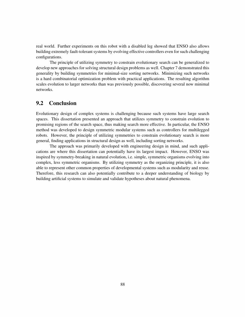
real world. Further experiments on this robot with a disabled leg showed that ENSO also allowsbuilding extremely fault-tolerant systems by evolving effective controllers even for such challengingconfigurations.

The principle of utilizing symmetry to constrain evolutionary search can be generalized todevelop new approaches for solving structural design problems as well. Chapter 7 demonstrated thisgenerality by building symmetries for minimal-size sorting networks. Minimizing such networksis a hard combinatorial optimization problem with practical applications. The resulting algorithmscales evolution to larger networks than was previously possible, discovering several now minimalnetworks.

9.2 Conclusion

Evolutionary design of complex systems is challenging because such systems have large searchspaces. This dissertation presented an approach that utilizes symmetry to constrain evolution topromising regions of the search space, thus making search more effective. In particular, the ENSOmethod was developed to design symmetric modular systems such as controllers for multileggedrobots. However, the principle of utilizing symmetries to constrain evolutionary search is moregeneral, finding applications in structural design as well, including sorting networks.

The approach was primarily developed with engineering design in mind, and such appli-cations are where this dissertation can potentially have its largest impact. However, ENSO wasinspired by symmetry-breaking in natural evolution, i.e. simple, symmetric organisms evolving intocomplex, less symmetric organisms. By utilizing symmetry as the organizing principle, it is alsoable to represent other common properties of developmental systems such as modularity and reuse.Therefore, this research can also potentially contribute to a deeper understanding of biology bybuilding artificial systems to simulate and validate hypotheses about natural phenomena.

88

Appendix A

Evolved Sorting Networks

This appendix lists examples of minimal-size sorting networks evolved by the algorithm describedin Chapter 7. For each example, the sequence of comparators is illustrated in a figure and also listedas pairs of horizontal lines numbered from top to bottom.

Figure A.1: Evolved 9-input network with 25 comparators: [3, 7], [1, 6], [2, 5], [8, 9], [1, 8], [2, 3], [4, 6],[5, 7], [6, 9], [2, 4], [7, 9], [1, 2], [5, 6], [3, 8], [4, 8], [4, 5], [6, 7], [2, 3], [2, 4], [7, 8], [5, 6], [3, 5], [6, 7],[3, 4], [5, 6].

89

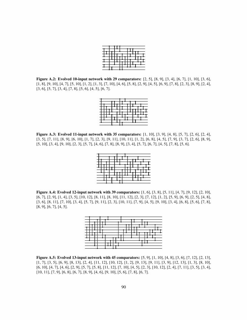
Figure A.2: Evolved 10-input network with 29 comparators: [2, 5], [8, 9], [3, 4], [6, 7], [1, 10], [3, 6],[1, 8], [9, 10], [4, 7], [5, 10], [1, 2], [1, 3], [7, 10], [4, 6], [5, 8], [2, 9], [4, 5], [6, 9], [7, 8], [2, 3], [8, 9], [2, 4],[3, 6], [5, 7], [3, 4], [7, 8], [5, 6], [4, 5], [6, 7].

Figure A.3: Evolved 11-input network with 35 comparators: [1, 10], [3, 9], [4, 8], [5, 7], [2, 6], [2, 4],[3, 5], [7, 11], [8, 9], [6, 10], [1, 7], [2, 3], [9, 11], [10, 11], [1, 2], [6, 8], [4, 5], [7, 9], [3, 7], [2, 6], [8, 9],[5, 10], [3, 4], [9, 10], [2, 3], [5, 7], [4, 6], [7, 8], [8, 9], [3, 4], [5, 7], [6, 7], [4, 5], [7, 8], [5, 6].

Figure A.4: Evolved 12-input network with 39 comparators: [1, 6], [3, 8], [5, 11], [4, 7], [9, 12], [2, 10],[6, 7], [2, 9], [1, 4], [3, 5], [10, 12], [8, 11], [8, 10], [11, 12], [2, 3], [7, 12], [1, 2], [5, 9], [6, 9], [2, 5], [4, 8],[3, 6], [8, 11], [7, 10], [3, 4], [5, 7], [9, 11], [2, 3], [10, 11], [7, 9], [4, 5], [9, 10], [3, 4], [6, 8], [5, 6], [7, 8],[8, 9], [6, 7], [4, 5].

Figure A.5: Evolved 13-input network with 45 comparators: [5, 9], [1, 10], [4, 8], [3, 6], [7, 12], [2, 13],[1, 7], [3, 5], [6, 9], [8, 13], [2, 4], [11, 12], [10, 12], [1, 2], [9, 13], [9, 11], [3, 9], [12, 13], [1, 3], [8, 10],[6, 10], [4, 7], [4, 6], [2, 9], [5, 7], [5, 8], [11, 12], [7, 10], [4, 5], [2, 3], [10, 12], [2, 4], [7, 11], [3, 5], [3, 4],[10, 11], [7, 9], [6, 8], [6, 7], [8, 9], [4, 6], [9, 10], [5, 6], [7, 8], [6, 7].

90

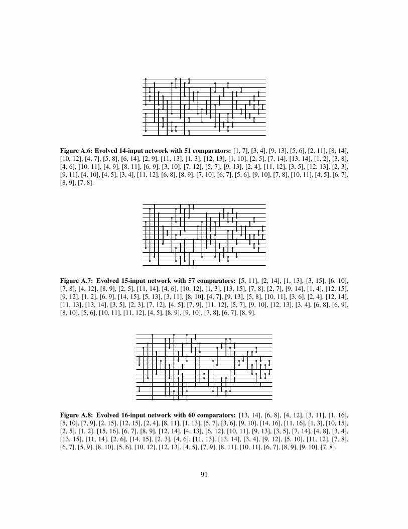
Figure A.6: Evolved 14-input network with 51 comparators: [1, 7], [3, 4], [9, 13], [5, 6], [2, 11], [8, 14],[10, 12], [4, 7], [5, 8], [6, 14], [2, 9], [11, 13], [1, 3], [12, 13], [1, 10], [2, 5], [7, 14], [13, 14], [1, 2], [3, 8],[4, 6], [10, 11], [4, 9], [8, 11], [6, 9], [3, 10], [7, 12], [5, 7], [9, 13], [2, 4], [11, 12], [3, 5], [12, 13], [2, 3],[9, 11], [4, 10], [4, 5], [3, 4], [11, 12], [6, 8], [8, 9], [7, 10], [6, 7], [5, 6], [9, 10], [7, 8], [10, 11], [4, 5], [6, 7],[8, 9], [7, 8].

Figure A.7: Evolved 15-input network with 57 comparators: [5, 11], [2, 14], [1, 13], [3, 15], [6, 10],[7, 8], [4, 12], [8, 9], [2, 5], [11, 14], [4, 6], [10, 12], [1, 3], [13, 15], [7, 8], [2, 7], [9, 14], [1, 4], [12, 15],[9, 12], [1, 2], [6, 9], [14, 15], [5, 13], [3, 11], [8, 10], [4, 7], [9, 13], [5, 8], [10, 11], [3, 6], [2, 4], [12, 14],[11, 13], [13, 14], [3, 5], [2, 3], [7, 12], [4, 5], [7, 9], [11, 12], [5, 7], [9, 10], [12, 13], [3, 4], [6, 8], [6, 9],[8, 10], [5, 6], [10, 11], [11, 12], [4, 5], [8, 9], [9, 10], [7, 8], [6, 7], [8, 9].

Figure A.8: Evolved 16-input network with 60 comparators: [13, 14], [6, 8], [4, 12], [3, 11], [1, 16],[5, 10], [7, 9], [2, 15], [12, 15], [2, 4], [8, 11], [1, 13], [5, 7], [3, 6], [9, 10], [14, 16], [11, 16], [1, 3], [10, 15],[2, 5], [1, 2], [15, 16], [6, 7], [8, 9], [12, 14], [4, 13], [6, 12], [10, 11], [9, 13], [3, 5], [7, 14], [4, 8], [3, 4],[13, 15], [11, 14], [2, 6], [14, 15], [2, 3], [4, 6], [11, 13], [13, 14], [3, 4], [9, 12], [5, 10], [11, 12], [7, 8],[6, 7], [5, 9], [8, 10], [5, 6], [10, 12], [12, 13], [4, 5], [7, 9], [8, 11], [10, 11], [6, 7], [8, 9], [9, 10], [7, 8].

91

Figure A.9: Evolved 17-input network with 71 comparators: [6, 12], [5, 10], [8, 13], [1, 15], [3, 17],[2, 16], [4, 9], [7, 14], [4, 11], [9, 14], [5, 8], [10, 13], [1, 3], [15, 17], [2, 7], [11, 16], [4, 6], [12, 14], [1, 5],[13, 17], [2, 4], [14, 16], [1, 2], [16, 17], [3, 10], [8, 15], [6, 11], [7, 12], [6, 8], [7, 9], [9, 11], [3, 4], [9, 15],[10, 12], [13, 14], [5, 7], [11, 15], [5, 6], [8, 10], [12, 14], [2, 3], [15, 16], [2, 9], [14, 16], [2, 5], [3, 6],[12, 15], [14, 15], [3, 5], [7, 13], [10, 13], [4, 11], [4, 9], [7, 8], [11, 13], [4, 7], [4, 5], [13, 14], [11, 12],[6, 7], [12, 13], [5, 6], [8, 9], [9, 10], [7, 9], [10, 12], [6, 8], [7, 8], [10, 11], [9, 10], [8, 9].

Figure A.10: Evolved 18-input network with 78 comparators: [5, 13], [6, 14], [1, 8], [11, 18], [3, 4],[15, 16], [7, 9], [10, 12], [2, 17], [3, 7], [12, 16], [2, 10], [9, 17], [5, 11], [8, 14], [4, 13], [6, 15], [1, 3],[16, 18], [2, 5], [14, 17], [1, 6], [13, 18], [1, 2], [17, 18], [4, 8], [11, 15], [7, 10], [9, 12], [3, 16], [4, 9],[10, 15], [5, 6], [13, 14], [7, 11], [3, 7], [8, 12], [2, 5], [14, 17], [15, 16], [3, 4], [12, 16], [16, 17], [2, 3],[12, 15], [4, 7], [14, 15], [4, 5], [15, 16], [3, 4], [6, 7], [12, 13], [8, 10], [9, 11], [10, 11], [8, 9], [6, 12], [7, 13],[11, 13], [6, 8], [13, 15], [4, 6], [11, 14], [5, 8], [13, 14], [5, 6], [9, 10], [7, 10], [9, 12], [10, 13], [6, 9], [7, 8],[11, 12], [7, 9], [10, 12], [8, 11], [10, 11], [8, 9].

92

Figure A.11: Evolved 19-input network with 86 comparators: [5, 11], [4, 13], [1, 17], [8, 15], [9, 12],[7, 14], [16, 18], [2, 6], [10, 19], [3, 6], [12, 17], [8, 10], [2, 3], [7, 16], [11, 13], [4, 5], [14, 18], [1, 9],[15, 19], [6, 17], [4, 8], [18, 19], [2, 7], [5, 16], [1, 2], [13, 17], [1, 4], [17, 19], [3, 12], [10, 11], [14, 15],[7, 9], [8, 14], [3, 10], [12, 16], [2, 8], [6, 11], [13, 18], [9, 15], [5, 7], [11, 15], [4, 5], [16, 17], [2, 3], [15, 18],[2, 4], [17, 18], [6, 8], [7, 14], [6, 7], [11, 16], [3, 5], [15, 16], [3, 6], [12, 13], [16, 17], [3, 4], [9, 10], [8, 14],[10, 13], [9, 12], [10, 11], [14, 15], [6, 9], [13, 15], [15, 16], [4, 6], [5, 7], [11, 14], [5, 9], [5, 6], [14, 15],[8, 12], [7, 12], [7, 10], [8, 9], [12, 13], [7, 8], [13, 14], [6, 7], [10, 11], [11, 12], [12, 13], [9, 10], [8, 9],[10, 11].

Figure A.12: Evolved 20-input network with 92 comparators: [3, 12], [9, 18], [1, 11], [10, 20], [5, 6],[15, 16], [4, 7], [14, 17], [2, 13], [8, 19], [4, 15], [6, 17], [1, 2], [19, 20], [5, 14], [7, 16], [8, 10], [11, 13],[3, 9], [12, 18], [5, 8], [13, 16], [1, 4], [17, 20], [1, 3], [18, 20], [1, 5], [16, 20], [2, 15], [6, 19], [9, 11],[10, 12], [7, 14], [6, 10], [11, 15], [2, 4], [17, 19], [7, 9], [12, 14], [3, 8], [13, 18], [2, 6], [2, 3], [15, 19], [5, 7],[14, 16], [18, 19], [16, 19], [2, 5], [4, 10], [11, 17], [3, 4], [17, 18], [14, 18], [3, 7], [16, 18], [3, 5], [8, 9],[12, 13], [6, 11], [10, 15], [9, 13], [8, 12], [4, 8], [13, 17], [4, 6], [15, 17], [16, 17], [4, 5], [6, 7], [14, 15],[15, 16], [5, 6], [11, 12], [9, 10], [12, 13], [8, 9], [8, 11], [10, 13], [6, 8], [13, 15], [10, 14], [7, 11], [7, 8],[11, 12], [13, 14], [9, 10], [10, 12], [12, 13], [9, 11], [8, 9], [10, 11].

93

Figure A.13: Evolved 21-input network with 103 comparators: [12, 21], [2, 3], [5, 17], [9, 11], [18, 20],[6, 8], [7, 19], [10, 14], [13, 15], [1, 4], [3, 14], [1, 5], [20, 21], [16, 19], [6, 12], [13, 16], [7, 18], [9, 10],[8, 15], [4, 17], [11, 19], [9, 13], [15, 17], [1, 7], [14, 21], [2, 6], [1, 9], [17, 19], [19, 21], [1, 2], [6, 12],[3, 20], [5, 16], [8, 11], [10, 18], [4, 12], [6, 10], [12, 14], [8, 13], [15, 18], [4, 7], [11, 20], [3, 5], [16, 17],[4, 8], [2, 6], [17, 20], [3, 9], [14, 19], [2, 4], [18, 19], [19, 20], [2, 3], [7, 13], [12, 16], [6, 7], [14, 18],[16, 17], [4, 9], [17, 18], [3, 6], [18, 19], [3, 4], [14, 16], [11, 15], [5, 10], [5, 8], [11, 12], [13, 15], [10, 15],[5, 11], [5, 6], [16, 17], [15, 18], [17, 18], [4, 5], [7, 9], [10, 12], [6, 7], [9, 11], [15, 16], [5, 6], [16, 17],[8, 13], [12, 13], [8, 10], [10, 11], [11, 13], [8, 9], [6, 8], [13, 16], [12, 14], [7, 9], [14, 15], [7, 8], [13, 15],[10, 12], [11, 14], [9, 12], [9, 10], [8, 9], [11, 12], [13, 14].

Figure A.14: Evolved 22-input network with 108 comparators: [11, 12], [3, 9], [14, 20], [4, 16], [7, 19],[2, 17], [6, 21], [1, 18], [5, 22], [8, 10], [13, 15], [1, 5], [18, 22], [4, 13], [10, 19], [2, 3], [20, 21], [8, 14],[9, 15], [6, 7], [16, 17], [6, 8], [15, 17], [2, 11], [12, 21], [1, 4], [19, 22], [1, 6], [17, 22], [1, 2], [21, 22], [7, 9],[14, 16], [3, 5], [18, 20], [10, 12], [11, 13], [3, 8], [15, 20], [4, 10], [13, 19], [7, 14], [9, 16], [5, 12], [11, 18],[6, 11], [12, 17], [4, 7], [16, 19], [2, 3], [20, 21], [2, 4], [19, 21], [2, 6], [17, 21], [3, 7], [16, 20], [12, 19],[3, 6], [17, 20], [4, 11], [3, 4], [19, 20], [10, 13], [5, 15], [8, 18], [9, 14], [13, 18], [5, 10], [14, 15], [8, 9],[5, 8], [15, 18], [5, 6], [17, 18], [18, 19], [4, 5], [7, 11], [12, 16], [6, 7], [16, 17], [5, 6], [17, 18], [10, 13],[9, 14], [11, 14], [9, 12], [8, 10], [13, 15], [8, 9], [14, 15], [15, 17], [6, 8], [10, 11], [12, 13], [7, 10], [13, 16],[15, 16], [7, 8], [9, 12], [11, 14], [9, 10], [13, 14], [8, 9], [14, 15], [11, 12], [12, 13], [10, 11].

94

Figure A.15: Evolved 23-input network with 118 comparators: [2, 21], [3, 22], [6, 14], [10, 18], [1, 8],[16, 23], [5, 12], [7, 13], [11, 17], [9, 19], [15, 20], [4, 9], [5, 15], [12, 19], [3, 7], [17, 21], [1, 10], [14, 23],[6, 16], [8, 18], [2, 11], [13, 22], [9, 20], [18, 23], [1, 6], [21, 22], [2, 3], [19, 20], [4, 5], [22, 23], [1, 2],[20, 23], [1, 4], [13, 14], [10, 11], [7, 16], [8, 17], [9, 12], [12, 15], [5, 12], [7, 9], [15, 17], [18, 21], [3, 6],[10, 13], [11, 14], [16, 19], [11, 12], [5, 8], [21, 22], [2, 3], [8, 16], [4, 10], [14, 20], [17, 19], [9, 15], [5, 7],[19, 22], [2, 5], [20, 22], [2, 4], [10, 11], [12, 14], [3, 7], [17, 21], [5, 10], [14, 19], [20, 21], [3, 4], [19, 21],[3, 5], [6, 18], [13, 15], [9, 13], [6, 8], [16, 18], [6, 9], [15, 18], [4, 6], [18, 20], [4, 5], [19, 20], [7, 11],[12, 17], [14, 17], [7, 10], [17, 18], [6, 7], [5, 6], [8, 10], [18, 19], [13, 16], [15, 16], [9, 13], [8, 9], [14, 16],[16, 18], [6, 8], [10, 11], [11, 15], [7, 12], [15, 17], [16, 17], [7, 8], [11, 12], [10, 13], [12, 14], [14, 15],[9, 10], [8, 9], [15, 16], [10, 11], [9, 10], [13, 15], [12, 13], [13, 14], [11, 12], [12, 13].

95

Figure A.16: Evolved 24-input network with 125 comparators: [6, 7], [18, 19], [5, 11], [14, 20], [2, 10],[15, 23], [9, 13], [12, 16], [4, 8], [17, 21], [1, 3], [22, 24], [2, 15], [10, 23], [6, 17], [8, 19], [4, 18], [7, 21],[1, 22], [3, 24], [5, 14], [11, 20], [9, 12], [13, 16], [4, 6], [19, 21], [1, 9], [16, 24], [2, 5], [20, 23], [2, 4],[21, 23], [15, 19], [1, 2], [23, 24], [3, 13], [12, 22], [7, 14], [11, 18], [8, 17], [3, 15], [10, 22], [9, 11], [14, 16],[7, 12], [13, 18], [5, 8], [17, 20], [6, 10], [19, 22], [3, 6], [2, 5], [20, 23], [16, 18], [7, 9], [21, 22], [3, 4],[18, 22], [3, 7], [2, 3], [22, 23], [16, 21], [4, 9], [5, 6], [19, 20], [18, 20], [5, 7], [21, 22], [3, 4], [20, 22],[3, 5], [11, 17], [8, 14], [10, 12], [13, 15], [10, 13], [15, 17], [8, 11], [12, 14], [12, 15], [14, 17], [8, 10], [4, 8],[17, 21], [4, 5], [20, 21], [6, 9], [16, 19], [18, 19], [6, 7], [17, 19], [6, 8], [19, 20], [5, 6], [7, 10], [11, 13],[11, 16], [13, 15], [14, 18], [11, 12], [7, 11], [15, 18], [18, 19], [6, 7], [15, 17], [12, 16], [9, 13], [8, 11],[17, 18], [7, 8], [15, 16], [9, 10], [13, 14], [9, 12], [14, 16], [16, 17], [8, 9], [9, 11], [10, 15], [12, 13], [10, 12],[13, 15], [14, 15], [12, 13], [10, 11].

96

Bibliography

Ajtai, M., Komlos, J., and Szemeredi, E. (1983). Sorting in c log n parallel steps. Combinatorica,3(1):1–19.

Alden, M. E. (2007). MARLEDA: Effective Distribution Estimation Through Markov RandomFields. PhD thesis, Department of Computer Sciences, The University of Texas at Austin. Tech-nical Report AI07-349.

Baddar, S. W. A. (2009). Finding Better Sorting Networks. PhD thesis, Kent State University.

Bastert, O. (2001). Stabilization Procedures and Applications. PhD thesis, Technische UniversitatMuchen.

Batcher, K. E. (1968). Sorting networks and their applications. In AFIPS Spring Joint ComputingConference, 307–314.

Beer, R. D., Chiel, H. J., and Sterling, L. S. (1989). Heterogeneous neural networks for adaptivebehavior in dynamic environments. In Advances in Neural Information Processing Systems 1,577–585. San Francisco, CA, USA: Morgan Kaufmann Publishers Inc.

Beer, R. D., and Gallagher, J. C. (1992). Evolving dynamical neural networks for adaptive behavior.Adaptive Behavior, 1(1):91–122.

Beineke, L., Wilson, R., and Cameron, P. (2004). Introduction. In Beineke, L. W., and Wilson, R. J.,editors, Topics in Algebraic Graph Theory, 1–29. New York, NY, USA: Cambridge UniversityPress.

Bengoetxea, E., Larranaga, P., Bloch, I., and Perchant, A. (2001). Estimation of distribution al-gorithms: A new evolutionary computation approach for graph matching problems. In EnergyMinimization Methods in Computer Vision and Pattern Recognition, 454–469. Springer.

Berryman, M. J., Allison, A., and Abbott, D. (2004). Optimizing genetic algorithm strategies forevolving networks. In White, L. B., editor, Noise in Communication, vol. 5473 of Proceedings ofSPIE, 122–130. Bellingham, WA, USA: SPIE.

Billard, A., and Ijspeert, A. J. (2000). Biologically inspired neural controllers for motor controlin a quadruped robot. In Proceedings of the International Joint Conference on Neural Networks(IJCNN 2000), 637–641.

97

http://nn.cs.utexas.edu/keyword?alden:phd07

http://nn.cs.utexas.edu/keyword?alden:phd07

http://rave.ohiolink.edu/etdc/view?acc_num

http://dx.doi.org.ezproxy.lib.utexas.edu/10.1007/3-540-44745-8_30

http://dx.doi.org.ezproxy.lib.utexas.edu/10.1007/3-540-44745-8_30

Boers, E. J. W., and Kuiper, H. (1992). Biological Metaphors and the Design of Modular Artifi-cial Neural Networks. Master’s thesis, Departments of Computer Science and Experimental andTheoretical Psychology at Leiden University, The Netherlands.

Bongard, J. C., and Lipson, H. (2004). Once more unto the breach: Co-evolving a robot and itssimulator. In Proceedings of the Ninth International Conference on the Simulation and Synthesisof Living Systems (ALIFE9), 57–62. MIT Press.

Bongard, J. C., and Pfeifer, R. (2001). Repeated structure and dissociation of genotypic and pheno-typic complexity in artificial ontogeny. In Spector, L., Goodman, E. D., Wu, A., Langdon, W. B.,Voigt, H.-M., Gen, M., Sen, S., Dorigo, M., Pezeshk, S., Garzon, M. H., and Burke, E., editors,Proceedings of the Genetic and Evolutionary Computation Conference, 829–836. San Francisco:Morgan Kaufmann.

Bongard, J. C., and Pfeifer, R. (2003). Evolving complete agents using artificial ontogeny. InMorpho-Functional Machines: The New Species (Designing Embodied Intelligence), 237–258.Springer-Verlag, Berlin.

Brading, K., and Castellani, E. (2008). Symmetry and symmetry breaking. In Zalta, E. N., editor,The Stanford Encyclopedia of Philosophy. The Metaphysics Research Lab, Center for the Studyof Language and Information, Stanford University.

Brooks, R. A. (1989). A robot that walks; emergent behaviors from a carefully evolved network.Technical Report AIM-1091, Massachusetts Institute of Technology, Cambridge, MA, USA.

Brooks, R. A. (1992). Artificial life and real robots. In Proceedings of the First European Confer-ence on Artificial Life, 3–10. MIT Press.

Brooks, R. A., and Maes, P., editors (1994). Proceedings of the Fourth International Workshop onthe Synthesis and Simulation of Living Systems (Artificial Life IV). Cambridge, MA: MIT Press.

Bull, L., Fogarty, T. C., and Snaith, M. (1995). Evolution in multi-agent systems: Evolving commu-nicating classifier systems for gait in a quadrupedal robot. In Proceedings of the 6th InternationalConference on Genetic Algorithms, 382–388. San Francisco, CA, USA: Morgan Kaufmann Pub-lishers Inc.

Cangelosi, A., Parisi, D., and Nolfi, S. (1994). Cell division and migration in a ‘genotype’ for neuralnetworks. Network: Computation in Neural Systems, 5:497–515.

Chakrabarti, C., and Wang, L.-Y. (1994). Novel sorting network-based architectures for rank orderfilters. IEEE Transactions on Very Large Scale Integration (VLSI) Systems, 2(4):502–507.

Chan, A., and Godsil, C. (1997). Symmetry and eigenvectors. In Hahn, G., and Sabidussi, G.,editors, Graph Symmetry: Algebraic Methods and Applications, 75–106. Springer.

Chauvin, Y., and Rumelhart, D. E., editors (1995). Backpropagation: Theory, Architectures, andApplications. Hillsdale, NJ: Erlbaum.

98

http://citeseer.nj.nec.com/boers92biological.html

http://citeseer.nj.nec.com/boers92biological.html

http://www-illigal.ge.uiuc.edu:8080/gecco-2001/

http://www-illigal.ge.uiuc.edu:8080/gecco-2001/

http://www.mpi-sb.mpg.de/services/library/proceedings/contents/alife94.html


http://kant.irmkant.rm.cnr.it/econets/cangelosi.migration.ps.Z

http://kant.irmkant.rm.cnr.it/econets/cangelosi.migration.ps.Z

Chung, K.-L., and Lin, Y.-K. (1997). A generalized pipelined median filter network. Signal Pro-cessing, 63(1):101 – 106.

Clark, J. E. (2004). Design, Simulation, and Stability of a Hexapedal Running Robot. PhD thesis,Department of Mechanical Engineering, Stanford University.

Clune, J., Beckmann, B. E., Ofria, C., and Pennock, R. T. (2009). Evolving coordinated quadrupedgaits with the HyperNEAT generative encoding. In Proceedings of the Eleventh conferenceon Congress on Evolutionary Computation (CEC’09), 2764–2771. Piscataway, NJ, USA: IEEEPress.

Collins, J. J., and Stewart, I. N. (1993). Coupled nonlinear oscillators and the symmetries of animalgaits. Journal of Nonlinear Science, 3(1):349–392.

Cornell Computational Synthesis Lab (2010). Cornell Computational Synthesis Lab (CCSL).http://ccsl.mae.cornell.edu/.

Deb, K., Agrawal, S., Pratab, A., and Meyarivan, T. (2000). A fast elitist non-dominated sortinggenetic algorithm for multi-objective optimization: NSGA-II. PPSN VI, 849–858.

Dellaert, F., and Beer, R. D. (1996). A developmental model for the evolution of complete au-tonomous agents. In Maes, P., Mataric, M. J., Meyer, J.-A., Pollack, J., and Wilson, S. W., editors,From Animals to Animats 4: Proceedings of the Fourth International Conference on Simulationof Adaptive Behavior. Cambridge, MA: MIT Press.

Edwards, R., and Glass, L. (2000). Combinatorial explosion in model gene networks. Chaos,10:691–704.

Fahlman, S. E., and Lebiere, C. (1990). The cascade-correlation learning architecture. In Touretzky(1990), 524–532.

Ferrell, C. (1994). Failure recognition and fault tolerance of an autonomous robot. Adaptive Behav-ior, 2(4):375–398.

Filliat, D., Kodjabachian, J., and Meyer, J.-A. (1999). Evolution of neural controllers for locomotionand obstacle avoidance in a six-legged robot. Connection Science, 11(3/4):225–242.

Floreano, D., and Mondada, F. (1998). Evolutionary neurocontrollers for autonomous mobilerobots. Neural Networks, 11:1461–1478.

Gao, L., Liu, S., and Dougal, R. A. (2002). Dynamic lithium-ion battery model for system simula-tion. IEEE Transactions on Components and Packaging Technologies, 25(3):495 – 505.

Gao, L., Sun, P., and Song, J. (2009). Clustering algorithms for detecting functional modules inprotein interaction networks. Journal of Bioinformatics and Computational Biology, 07(01):217.

GAP (2007). GAP – groups, algorithms, and programming. http://www.gap-system.org.

99

http://www.sciencedirect.com/science/article/B6V18-3SNYT5C-1B/2/38110bb682311c8cc6169b64b233dac5

http://ccsl.mae.cornell.edu/

http://ccsl.mae.cornell.edu/

http://citeseer.nj.nec.com/dellaert96developmental.html

http://citeseer.nj.nec.com/dellaert96developmental.html

http://www.worldscinet.com/jbcb/07/0701/S0219720009004023.html

http://www.worldscinet.com/jbcb/07/0701/S0219720009004023.html

http://www.gap-system.org

http://www.gap-system.org

Garcia-Bellido, A. (1996). Symmetries throughout organic evolution. PNAS, 93(25):14229–14232.

Golubitsky, M., Shiau, L. J., and Torok, A. (2003). Bifurcation on the visual cortex with weaklyanisotropic lateral coupling. SIAM Journal on Applied Dynamical Systems, 2(2):97–143.

Golubitsky, M., and Stewart, I. (2002). Patterns of oscillation in coupled cell systems. In Newton, P.,Holmes, P., and Weinstein, A., editors, Geometry, Mechanics, and Dynamics: Volume in Honorof the 60th Birthday of J. E. Marsden, chapter 8, 243–286. Springer.

Gomez, F., and Miikkulainen, R. (2004). Transfer of neuroevolved controllers in unstable domains.In Proceedings of the Genetic and Evolutionary Computation Conference. Berlin: Springer.

Graham, L., and Oppacher, F. (2006). Symmetric comparator pairs in the initialization of geneticalgorithm populations for sorting networks. IEEE Congress on Evolutionary Computation, 2006(CEC 2006), 2845–2850.

Gruau, F. (1994a). Automatic definition of modular neural networks. Adaptive Behavior, 3(2):151–183.

Gruau, F. (1994b). Neural Network Synthesis Using Cellular Encoding and the Genetic Algorithm.PhD thesis, Ecole Normale Superieure de Lyon, France.

Gruau, F., and Whitley, D. (1993). Adding learning to the cellular development of neural networks:Evolution and the Baldwin effect. Evolutionary Computation, 1:213–233.

Gruau, F., Whitley, D., and Pyeatt, L. (1996). A comparison between cellular encoding and directencoding for genetic neural networks. In Koza, J. R., Goldberg, D. E., Fogel, D. B., and Riolo,R. L., editors, Genetic Programming 1996: Proceedings of the First Annual Conference, 81–89.Cambridge, MA: MIT Press.

Gunter, C. A., Ngair, T.-H., and Subramanian, D. (1996). Sets as anti-chains. In ASIAN ’96: Pro-ceedings of the Second Asian Computing Science Conference on Concurrency and Parallelism,Programming, Networking, and Security, 116–128. London, UK: Springer-Verlag.

Heylighen, F. (1999). The growth of structural and functional complexity during evolution. InHeylighen, F., Bollen, J., Riegler, A., and Riegler, A., editors, The Evolution of Complexity: TheViolet Book of ’Einstein Meets Magritte’, chapter 2, 17–44. Springer.

Hiasat, A., and Hasan, O. (2003). Bit-serial architecture for rank order and stack filters. Integration,the VLSI Journal, 36(1-2):3 – 12.

Hillis, W. D. (1991). Co-evolving parasites improve simulated evolution as an optimization pro-cedure. In Farmer, J. D., Langton, C., Rasmussen, S., and Taylor, C., editors, Artificial Life II.Reading, MA: Addison-Wesley.

Holmes, P., Full, R. J., Koditschek, D., and Guckenheimer, J. (2006). The dynamics of leggedlocomotion: Models, analyses, and challenges. SIAM Review, 48(2):207–304.

100

http://nn.cs.utexas.edu/keyword?gomez:gecco04

http://citeseer.nj.nec.com/frederic94neural.html

http://www.sciencedirect.com/science/article/B6V1M-48NKGY5-1/2/53c0e6c9dfb4ef44292e616c4eab3356

Hornby, G. S., Fujita, M., Takamura, S., Yamamoto, T., and Hanagata, O. (1999). Autonomousevolution of gaits with the sony quadruped robot. In Proceedings of the Genetic and EvolutionaryComputation Conference (GECCO), 1297–1304.

Hornby, G. S., and Pollack, J. B. (2002). Creating high-level components with a generative repre-sentation for body-brain evolution. Artificial Life, 8(3).

Hornby, G. S., Takamura, S., Yokono, J., Hanagata, O., Yamamoto, T., and Fujita, M. (2000). Evolv-ing robust gaits with AIBO. In Proceedings of the IEEE International Conference on Roboticsand Automation, vol. 3, 3040–3045.

Ijspeert, A. J. (2008). Central pattern generators for locomotion control in animals and robots: Areview. Neural Networks, 21(4):642–653.

Jakobi, N. (1998). Minimal Simulations for Evolutionary Robotics. PhD thesis, School of Cognitiveand Computing Sciences, University of Sussex.

Jakobi, N., Husbands, P., and Harvey, I. (1995). Noise and the reality gap: The use of simulationin evolutionary robotics. In Moran, F., Moreno, A., Merelo, J., and Chacon, P., editors, Advancesin Artificial Life, vol. 929 of Lecture Notes in Computer Science, 704–720. Springer Berlin /Heidelberg.

Juille, H. (1995). Evolution of non-deterministic incremental algorithms as a new approach forsearch in state spaces. In Proceedings of the 6th International Conference on Genetic Algorithms,351–358. San Francisco, CA, USA: Morgan Kaufmann Publishers Inc.

Kauffman, S. A. (1993). The Origins of Order. New York: Oxford University Press.

Kepes, F., editor (2007). Biological Networks. World Scientific.

Kimura, H., Akiyama, S., and Sakurama, K. (1999). Realization of dynamic walking and runningof the quadruped using neural oscillator. Autonomous Robots, 7(3):247–258.

Kipfer, P., Segal, M., and Westermann, R. (2004). Uberflow: A gpu-based particle engine. In HWWS’04: Proceedings of the ACM SIGGRAPH/EUROGRAPHICS conference on Graphics hardware,115–122. New York, NY, USA: ACM.

Kitano, H. (1990). Designing neural networks using genetic algorithms with graph generationsystem. Complex Systems, 4:461–476.

Knuth, D. E. (1998). Art of Computer Programming: Sorting and Searching, vol. 3. Addison-Wesley Professional. Second edition.

Koditschek, D. E., Full, R. J., and Buehler, M. (2004). Mechanical aspects of legged locomotioncontrol. Arthropod Structure and Development, 33(3):251–272.

Kodjabachian, J., and Meyer, J.-A. (1998). Evolution and development of modular control architec-tures for 1D locomotion in six-legged animats. Connection Science, 10:211–237.

101

http://www.demo.cs.brandeis.edu/papers/hornby_alife02.pdf

http://www.demo.cs.brandeis.edu/papers/hornby_alife02.pdf

http://dx.doi.org/10.1007/3-540-59496-5_337

http://dx.doi.org/10.1007/3-540-59496-5_337

Kohl, N., and Stone, P. (2004a). Machine learning for fast quadrupedal locomotion. In NineteenthNational Conference on Artificial Intelligence.

Kohl, N., and Stone, P. (2004b). Policy gradient reinforcement learning for fast quadrupedal lo-comotion. In Proceedings of the IEEE International Conference on Robotics and Automation,vol. 3, 2619–2624.

Koos, S., Mouret, J.-B., and Doncieux, S. (2010). Crossing the reality gap in evolutionary roboticsby promoting transferable controllers. In GECCO ’10: Proceedings of the 12th annual conferenceon Genetic and evolutionary computation, 119–126. New York, NY, USA: ACM.

Korenek, J., and Sekanina, L. (2005). Intrinsic evolution of sorting networks: A novel completehardware implementation for FPGAs. In Evolvable Systems: From Biology to Hardware, 46–55.Springer.

Korshunov, A. D. (2003). Monotone boolean functions. Russian Mathematical Surveys, 58(5):929.

Kovacs, A. (1986). Spontaneous symmetry breaking in biological systems. Origins of Life andEvolution of Biospheres, 16:429–430.

Koza, J. R., Goldberg, D. E., Fogel, D. B., and Riolo, R. L., editors (1996). Genetic Programming1996. Cambridge, MA: MIT Press.

Koza, J. R., Koza, J. R., Forest H. Bennett, I., Forest H. Bennett, I., Hutchings, J. L., Bade, S. L.,Keane, M. A., and Andre, D. (1998). Evolving computer programs using rapidly reconfigurablefield-programmable gate arrays and genetic programming. In FPGA ’98: Proceedings of the 1998ACM/SIGDA Sixth International Symposium on Field Programmable Gate Arrays, 209–219. NewYork, NY, USA: ACM.

le Cun, Y., Denker, J. S., and Solla, S. A. (1990). Optimal brain damage. In Touretzky (1990),598–605.

Leighton, T., and Plaxton, C. G. (1990). A (fairly) simple circuit that (usually) sorts. In SFCS ’90:Proceedings of the 31st Annual Symposium on Foundations of Computer Science, 264–274 vol.1.Washington, DC, USA: IEEE Computer Society.

Lindenmayer, A. (1968). Mathematical models for cellular interaction in development parts I andII. Journal of Theoretical Biology, 18:280–299 and 300–315.

Lipson, H., Bongard, J., Zykov, V., and Malone, E. (2006). Evolutionary robotics for legged ma-chines: From simulation to physical reality. In Proceedings of the 9th International Conferenceon Intelligent Autonomous Systems., 11–18.

Luke, S., and Spector, L. (1996). Evolving graphs and networks with edge encoding: Preliminaryreport. In Koza, J. R., editor, Late-Breaking Papers of Genetic Programming 1996. StanfordBookstore.

102

http://dx.doi.org.ezproxy.lib.utexas.edu/10.1007/11549703_5

http://dx.doi.org.ezproxy.lib.utexas.edu/10.1007/11549703_5

http://stacks.iop.org/0036-0279/58/i=5/a=R02

http://dx.doi.org/10.1007/BF02422114

http://citeseer.nj.nec.com/128010.html

http://citeseer.nj.nec.com/128010.html

Martindale, M. Q., and Henry, J. Q. (1998). The development of radial and biradial symmetry: Theevolution of bilaterality. American Zoologist, 38(4):672–684.

Mataric, M., and Cliff, D. (1996). Challenges in evolving controllers for physical robots. Roboticsand Autonomous Systems, 19(1):67–83.

McFarlane, D. (1998). Modular distributed manufacturing systems and the implications for inte-grated control. In IEE Colloquium on Choosing the Right Control Structure for Your Process(Digest No. 1998/280).

Mehta, D. P., and Sahni, S. (2005). Handbook of data structures and applications. CRC Press.

Miglino, O., Lund, H. H., and Nolfi, S. (1995). Evolving mobile robots in simulated and realenvironments. Artificial Life, 2:417–434.

Miller, J. F. (2004). Evolving a self-repairing, self-regulating, French flag organism. In Proceed-ings of the Genetic and Evolutionary Computation Conference (GECCO-2004). Berlin: SpringerVerlag.

Muhlenbein, H., and Hons, R. (2005). The estimation of distributions and the minimum relativeentropy principle. Evolutionary Computation, 13(1):1–27.

Murtagh, F. (2002). Clustering in massive data sets. In Abello, J., Pardalos, P. M., and Resende,M. G. C., editors, Handbook of Massive Data Sets, chapter 14, 501–543. Norwell, MA, USA:Kluwer Academic Publishers.

Nolfi, S., Floreano, D., Miglino, O., and Mondada, F. (1994). How to evolve autonomous robots:Different approaches in evolutionary robotics. In Brooks and Maes (1994), 190–197.

Objet Eden 260V (2010). Objet Eden 260V. http://www.objet.com/3D-Printer/Eden260V/.

ODE (2007). ODE: Open dynamics engine. http://www.ode.org/.

OGRE (2007). OGRE: Object-oriented graphics rendering engine. http://www.ogre3d.org/.

OPAL (2007). OPAL: Open physics abstraction layer. http://opal.sourceforge.net/.

Open BEAGLE (2007). Open BEAGLE. http://beagle.gel.ulaval.ca/.

Palmer, A. R. (2004). Symmetry breaking and the evolution of development. Science, 306:828–833.

Pinto, C. M. A., and Golubitsky, M. (2006). Central pattern generators for bipedal locomotion.Journal of Mathematical Biology, 53(3):474–489.

Raibert, M. H. (1986). Legged robots. Communications of the ACM, 29(6):499–514.

103

http://www.ncbi.nlm.nih.gov/entrez/query.fcgi?cmd=retrieve&db=pubmed&dopt=abstract&list_uids=8942055

http://www.ncbi.nlm.nih.gov/entrez/query.fcgi?cmd=retrieve&db=pubmed&dopt=abstract&list_uids=8942055

http://www.elec.york.ac.uk/intsys/users/jfm7/gecco2004.pdf



http://www.objet.com/3D-Printer/Eden260V/



http://www.ode.org/

http://www.ode.org/

http://www.ogre3d.org/



http://opal.sourceforge.net/

http://opal.sourceforge.net/

http://beagle.gel.ulaval.ca/

http://beagle.gel.ulaval.ca/

Raibert, M. H., Chepponis, M., and H. Benjamin Brown, J. (1986). Running on four legs as thoughthey were one. IEEE Journal of Robotics and Automation, 2(2):70–82.

Righetti, L., and Ijspeert, A. J. (2008). Pattern generators with sensory feedback for the control ofquadruped locomotion. In Proceedings of the 2008 IEEE International Conference on Roboticsand Automation (ICRA 2008), 819–824.

Robotis (2010). Robotis. http://www.robotis.com/.

Rumelhart, D. E., Hinton, G. E., and Williams, R. J. (1986). Learning internal representationsby error propagation. In Rumelhart, D. E., and McClelland, J. L., editors, Parallel DistributedProcessing: Explorations in the Microstructure of Cognition, Vol. 1: Foundations, 318–362.Cambridge, MA: MIT Press.

Seo, K., and Slotine, J. J. E. (2007). Models for global synchronization in CPG-based locomotion.In Proceedings of the 2007 IEEE International Conference on Robotics and Automation, 281–286.

Seo, S.-W., yun Feng, T., and Kim, Y. (1993). A simulation scheme in rearrangeable networks. InProceedings of the 36th Midwest Symposium on Circuits and Systems, 177 – 180 vol. 1.

Shastri, S. V. (1997). A biologically consistent model of legged locomotion gaits. BiologicalCybernetics, 76(6):429–440.

Shmulevich, I., Sellke, T. M., Gabbouj, M., and Coyle, E. J. (1995). Stack filters and free distributivelattices. In Proceedings of the 1995 IEEE Workshop on Nonlinear Signal and Image Processing,927–930. IEEE Computer Society.

Siebel, N. T., and Sommer, G. (2007). Evolutionary reinforcement learning of artificial neuralnetworks. International Journal of Hybrid Intelligent Systems, 4(3):171–183.

Sims, K. (1994a). Evolving 3D morphology and behavior by competition. In Brooks and Maes(1994), 28–39.

Sims, K. (1994b). Evolving 3D morphology and behavior by competition. In Brooks, R. A.,and Maes, P., editors, Proceedings of the Fourth International Workshop on the Synthesis andSimulation of Living Systems (Artificial Life IV), 28–39. Cambridge, MA: MIT Press.

SolidWorks (2010). SolidWorks. http://www.solidworks.com/.

Stanley, K. (2007). Compositional pattern producing networks: A novel abstraction of development.Genetic Programming and Evolvable Machines, 8(2):131–162.

Stanley, K. O., D’Ambrosio, D. B., and Gauci, J. (2009). A Hypercube-Based encoding for evolvingLarge-Scale neural networks. Artificial Life, 15(2):185–212.

Stanley, K. O., and Miikkulainen, R. (2003). A taxonomy for artificial embryogeny. Artificial Life,9(2):93–130.

104

http://www.robotis.com/

http://www.robotis.com/



http://www.solidworks.com/

http://www.solidworks.com/

http://nn.cs.utexas.edu/keyword?stanley:alife03

Stanley, K. O., and Miikkulainen, R. (2004). Competitive coevolution through evolutionary com-plexification. Journal of Artificial Intelligence Research, 21:63–100.

Steiner, T., Jin, Y., and Sendhoff, B. (2009). Vector field embryogeny. PLoS ONE, 4(12):e8177.

Stone, P., and Veloso, M. (2000). Multiagent systems: A survey from a machine learning perspec-tive. Autonomous Robots, 8(3):345–383.

Tellez, R. A., Angulo, C., and Pardo, D. E. (2006). Evolving the walking behaviour of a 12DOF quadruped using a distributed neural architecture. In Biologically Inspired Approachesto Advanced Information Technology, Lecture Notes in Computer Science 3853, 5–19. Berlin:Springer.

Touretzky, D. S., editor (1990). Advances in Neural Information Processing Systems 2. San Fran-cisco: Morgan Kaufmann.

Watson, R. A., Ficici, S. G., and Pollack, J. B. (2002). Embodied evolution: Distributing an evolu-tionary algorithm in a population of robots. Robotics and Autonomous Systems, 39(1):1 – 18.

Watson, R. A., and Jansen, T. (2007). A building-block royal road where crossover is provablyessential. In Proceedings of the 9th annual conference on Genetic and evolutionary computation(GECCO ’07), 1452–1459. New York, NY, USA: ACM.

Yeh, Y.-M., and Feng, T.-y. (1992). On a class of rearrangeable networks. IEEE Transactions onComputers, 41(11):1361–1379.

Zagal, J. C., and Ruiz-Del-Solar, J. (2007). Combining simulation and reality in evolutionaryrobotics. Journal of Intelligent and Robotic Systems, 50(1):19–39.

Zhang, S. S., Xu, K., and Jow, T. R. (2003). The low temperature performance of li-ion batteries.Journal of Power Sources, 115(1):137 – 140.

Zykov, V., Bongard, J., and Lipson, H. (2004). Evolving dynamic gaits on a physical robot. InProceedings of the Genetic and Evolutionary Computation Conference, Late-Breaking Papers.

105

http://nn.cs.utexas.edu/keyword?stanley:jair04

http://nn.cs.utexas.edu/keyword?stanley:jair04

http://www.sciencedirect.com/science/article/B6TH1-47JCRT5-2/2/ba618d9d10f2bc31473b7aca3bdfb151

Vita

Vinod K. Valsalam entered the Indian Institute of Technology (IIT), Madras, India in 1992 and grad-

uated with a Bachelor of Technology degree in Aerospace Engineering in 1996. After graduating

from IIT, he moved to Starkville, Mississippi, where he studied Computational Engineering at Mis-

sissippi State University, eventually graduating with a Master of Science degree in 1998. Thereafter,

he worked as a researcher in Computer Science at Mississippi State University. In 2002, he entered

the University of Texas at Austin, Texas to pursue a doctorate degree in Computer Science.

Permanent Address: Department of Computer SciencesThe University of Texas at AustinAustin, TX [email protected]://www.cs.utexas.edu/users/vkv/

This dissertation was typeset with LATEX 2ε1 by the author.

1LATEX 2ε is an extension of LATEX. LATEX is a collection of macros for TEX. TEX is a trademark of the AmericanMathematical Society. The macros used in formatting this dissertation were written by Dinesh Das, Department ofComputer Sciences, The University of Texas at Austin, and extended by Bert Kay, James A. Bednar, and Ayman El-Khashab.

106

utilizing symmetry in evolutionary design

Documents