University of Arkansas, FayettevilleScholarWorks@UARK

Theses and Dissertations

12-2018

Utilizing the HVSR Second Peak for Surface WaveInversions in the Mississippi EmbaymentAshraf Kamal HimelUniversity of Arkansas, Fayetteville

Follow this and additional works at: https://scholarworks.uark.edu/etd

Part of the Civil Engineering Commons, Geophysics and Seismology Commons, GeotechnicalEngineering Commons, and the Structural Engineering Commons

This Thesis is brought to you for free and open access by ScholarWorks@UARK. It has been accepted for inclusion in Theses and Dissertations by anauthorized administrator of ScholarWorks@UARK. For more information, please contact scholar@uark.edu, ccmiddle@uark.edu.

Recommended CitationHimel, Ashraf Kamal, "Utilizing the HVSR Second Peak for Surface Wave Inversions in the Mississippi Embayment" (2018). Thesesand Dissertations. 3025.https://scholarworks.uark.edu/etd/3025

Utilizing the HVSR Second Peak for Surface Wave Inversions in the Mississippi Embayment

A thesis submitted in partial fulfillment

of the requirements for the degree of

Master of Science in Civil Engineering

by

Ashraf Kamal Himel

Bangladesh University of Engineering and Technology

Bachelor of Science in Civil Engineering, 2014

December 2018

University of Arkansas

This thesis is approved for recommendation to the Graduate Council.

__________________________________

Clinton Wood, Ph.D.

Thesis Director

__________________________________

Michelle Lee Barry, Ph.D.

Committee Member

__________________________________

Sarah Vavrik Hernandez, Ph.D.

Committee Member

Abstract

Ambient noise data from 24 sites within the Mississippi Embayment were analyzed to

estimate the fundamental frequency using the horizontal to vertical spectral ratio (HVSR)

method. The fundamental frequency ranged from 0.17 to 3.43 Hz for the tested sites. At

seventeen of the sites, a second higher frequency HVSR peak, which ranged from 0.617 Hz

to 2.154 Hz, was observed in addition to the fundamental HVSR peak. The second peak

frequency in the HVSR curve has been attributed by previous researchers as either an odd

harmonic of the fundamental peak or a shallow impedance contrast from the Memphis sand

layer in the Mississippi embayment. Shear wave transfer functions are compared for select

sites with the HVSR curves and geologic boring logs are analyzed to determine which

cause is most likely. Finally, a full scale inversion of active and passive surface wave data

is carried out at one site using the HVSR fundamental frequency to constrain the bedrock

depth and the second peak frequency to constrain the shallow impedance contrast depth to

demonstrate the usefulness of the HVSR second peak.

©2018 by Ashraf Kamal Himel

All Rights Reserved

Acknowledgement

I would like to sincerely thank my supervisor Dr. Clinton Wood. He has been very

supportive during this whole journey. I have learned a lot of things in the field of earthquake

engineering from him. Finishing up the thesis would not have been possible without his

guidance. I am thankful to get the opportunity to work with him.

I would like to thank Dr. Sarah Vavrik Hernandez and Dr. Michelle L. Barry for serving as

my thesis committee members. Their teaching has always helped me during my research. I

would also thank my teammates in Geotechnical Earthquake Engineering Lab of University of

Arkansas.

Dedication

This thesis is dedicated to my family. My father, Abser Kamal has been a great mentor for

me throughout my life. My mother, Hasina Jahan has always been beside me. My fiancé, Disha

has been patient and supportive the whole time. I would also like to thank my sisters for their

continuous support.

Table of Contents

1.0 Introduction: .............................................................................................................................. 1

2.0 Mississippi Embayment Geology ............................................................................................. 4

3.0 Testing Methodology and Data Processing .............................................................................. 6

3.1 Testing Methodology: ........................................................................................................... 8

3.2 HVSR Processing: ................................................................................................................. 9

4.0 HVSR Results ........................................................................................................................... 9

5.0 Inversion Results at Manila, AR ............................................................................................. 18

6.0 Conclusion: ............................................................................................................................. 26

References: .................................................................................................................................... 27

List of Tables

Table 1 Site locations and Bedrock depth (Ramirez et al. 2012).................................................... 7

Table 2 Second peak frequency and fundamental frequency along with their ratio, for the sites

with second peak . ......................................................................................................................... 17

List of Figures

Figure 1. Location of HVSR measurement sites in the Mississippi Embayment along with the

seismic stations and boreholes from Ryling (1960) used in this study. .......................................... 6

Figure 2: HVSR curve for the 15 NEA sites in the study compared with the theoretical shear

wave transfer function. The associated peaks are highlighted. ..................................................... 11

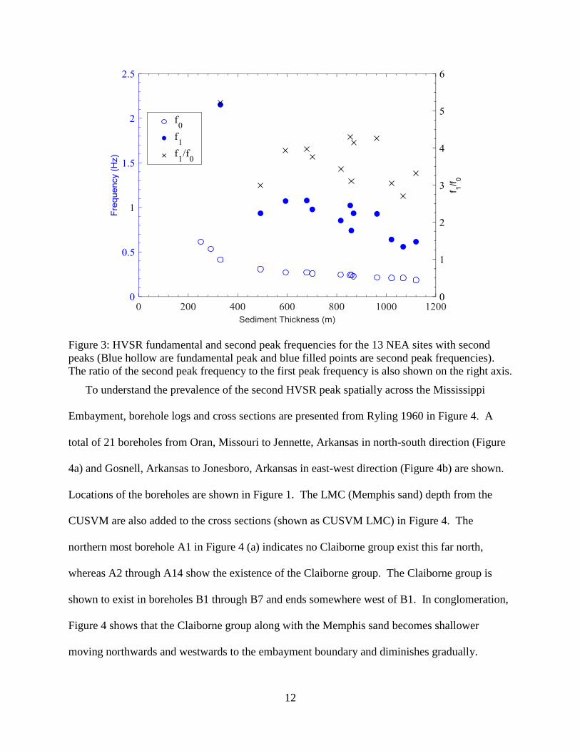
Figure 3: HVSR fundamental and second peak frequencies for the 13 NEA sites with second

peaks (Blue hollow are fundamental peak and blue filled points are second peak frequencies).

The ratio of the second peak frequency to the first peak frequency is also shown on the right axis.

....................................................................................................................................................... 12

Figure 4: Generalized geologic cross section of the Mississippi embayment from boreholes

originally presented in Ryling (1960): (a) North-South cross section for boreholes A1 – A14 and

(b) East-West cross section for boreholes B1 – B7. ..................................................................... 14

Figure 5: HVSR result of seismic stations EPRM, CHRM, CBMO, and MCIL......................... 15

Figure 6: HVSR results of the Additional Sites along the western edge of the Mississippi

Embayment. .................................................................................................................................. 16

Figure 7: Median Vs profiles of the 83 m model, 131 m model and 171 m model along with the

1000 Vs best profiles are shown. For each model, the estimated Memphis sand depth is shown

with the thick black line. Reference Vs profiles of Lin et al., 2014 for different soil types are

provided for comparison ............................................................................................................... 22

Figure 8: Rayleigh (a) and Love (b) dispersion curves, respectively. Green, red, and blue are

for 83 m model, 131 m model, and 171 m model, respectively. Solid line, dotted line and dashed

line are for fundamental mode, first higher mode and second higher mode of theoretical

dispersion curves, respectively. The black dots are experimental dispersion data. The inset in (a)

shows an enhanced image of the fundamental mode dispersion data from 0.5 Hz to 2.5 Hz. The

inset shows the separation of 131 m and 171 m model fundamental from the 83 m fundamental

mode at 1.77 Hz and following the experimental data. ................................................................ 23

Figure 9: Shear wave transfer function and theoretical ellipticity curve for each model along

with the Manila HVSR respectively for the 83 m model (a), 131 m model (b), and 171 m model

(c). ................................................................................................................................................. 25

1

1.0 Introduction:

The horizontal to vertical spectral ratio (HVSR) method, also known as the Nakamura’s

method (Nakamura 1989) is widely accepted as a tool to evaluate site effects (Guéguen et al.

2000). The HVSR peak frequency emulates the resonance frequency or fundamental frequency

(f0) of sediments above a strong impedance contrast and is equated to the shear wave

fundamental frequency (Field and Jacob 1993). The peak frequency is related to the sediment

thickness, while the amplitude is related to the shear wave velocity contrast between the top

sediments and stiff base material (Guéguen et al. 1998). While at many sites one primary peak is

often observed in the HVSR curve from only one major impedance contrast (Bonnefoy-Claudet

et al., 2008), the presence of two interfaces with significant impedance contrasts may generate

two peaks in the HVSR curve (Guéguen et al., 2000).

Two peaks in the HVSR curve have been observed in a number of locations around the

world. Zaslavsky et al., (2007) correlated the HVSR first peak frequency with the limestone

bedrock and the second peak frequency with the shallow softer alluvial sediments in Zevulun

plain, Israel. They showed that the HVSR second peak varied from 17 Hz down to 4 Hz,

matching the increase of alluvial layer thickness from 2 m to 15 m. Macau et al. (2015)

conducted a study on the effect of Quaternary deposits on HVSR at Llobregat river delta, located

to the south of Barcelona. In this study, they detected two impedance contrasts along with two

peaks in the HVSR curves. The first peak was correlated with the deeper impedance contrast

between soft sediment and bedrock, while the second peak was correlated with the shallow

impedance contrast between soft clay and gravel, concluding that the structure of shallow

quaternary layer can change the shape of H/V ratio by producing two clear peaks. Wotherspoon

et al. (2018) showed that the first HVSR peak in the Canterbury Plains, New Zealand was the

2

result of basement rock, while the second HVSR peak was correlated with a soft sand layer over

a stiff gravel layer located 10-40 m below the surface.

The existence of a second HVSR peak can also have a significant influence on the seismic

site effects for a particular location. For Pujili (Ecuador), the damage distribution due to the Mw

5.7 earthquake in 1996 showed most of the damaged buildings had similar natural frequency as

the HVSR second peak frequency. The second peak frequency in Pujili was found to be the

resonant frequency of a superficial thin layer (Field and Jacob 1993). The damage due to the

earthquake on May 21, 2003 hitting the eastern coast of Algiers also demonstrated a similar

condition. The first peak, around 1 Hz in the HVSR curve, could not explain the building

collapses, which had natural frequencies in the range of 3 – 4 Hz. A second HVSR peak around

3 Hz was observed in this case, which was correlated with the shallow impedance contrast

between quaternary and Mio-Pliocene layer (Dunand et al., 2004, Guillier et al., 2005).

The Mississippi embayment, situated in the Central United States, is a deep sedimentary

basin in which two HVSR peaks are often observed (Rosenblad and Goetz 2010 Bodin et al.,

2001, Wood et al., 2018, Guo and Aydin 2016, Guo et al., 2014, Carpenter et al., 2018). Bodin

et al. 2001 hypothesized that the second peak frequency (f1), is a harmonic of the fundamental

peak as the ratio f1/f0 was found to be near 3 and they could not identify an impedance contrast

strong enough to cause the second peak. Moreover, Goetz (2009) generated shear wave transfer

functions using Vs profiles from Rosenblad et al., 2010 to show that the shear wave transfer

function second peak is in good agreement (<10%) with the measured HVSR second peak. They

suggested that this could be a reason to consider the second peak frequency as a higher mode of

shear wave resonance. However, they also used the shear wave transfer function down to the

Memphis sand layer to show a relationship of decreasing resonance frequency with increasing

3

depth to the top of Memphis sand, indicating that the velocity contrast also could be the cause of

second peak frequency observed in the HVSR across the embayment similar to that observed in

many other basins around the globe. There is still uncertainty regarding the cause of the second

higher frequency HVSR peak observed throughout the embayment primarily due to the fact that

the higher frequency HVSR peak is often about three times the fundamental HVSR peak

associated with the bedrock formation, but also that the depth to the Memphis sand layer (the

presumed shallow impedance contrast) often decreases at a similar rate to the bedrock depth

across the embayment. This make is difficult to isolate the true cause of the second HVSR peak

across the region. Regardless of the cause of the second HVSR peak, the site effects which result

as a function of the amplification at the HVSR second peak frequency play a key role in the

seismic hazard of the region. However, if the second peak is a result of an impedance contrast at

the top of the Memphis Sand, this HVSR peak can be used in the solution of the inverse problem

in surface wave methods through a joint inversion to constrain the VS of the sediments, resulting

in a more accurate Vs profile (Scherbaum et al. 2003). Therefore, aiding in the assessment of

seismic hazard in the region.

In this paper, the HVSR second peak frequency observed in the Mississippi embayment is

associated with the shallow impedance contrast from the Memphis sand and the ability to use

this second HVSR peak frequency along with dispersion data from surface wave methods to

resolve the depth to the Memphis sand is demonstrated. Direct ambient noise measurements are

used to compute HVSRs at 15 sites across North East Arkansas and then compared to shear wave

transfer functions computed using VS profiles from Wood et al. (2018). Next HVSRs are

computed at nine sites at the western and northern edges of the embayment and compared to

boring logs and geologic cross sections which indicate the Memphis sand layer no longer exist

4

along the basin edges. Finally, the use of the HVSR second peak to constrain the inversion of

active and passive surface wave dispersion data is demonstrated for a site within the embayment.

2.0 Mississippi Embayment Geology

The Mississippi embayment is a southward plunging syncline, with its axis closely tracing

the course of the Mississippi river (Mento et al. 1986). The embayment has a rift type crustal

structure (Ginzburg et al. 1983) and the subsidence of the rift formed the Reelfoot Basin in early

Paleozoic (Schwalb 1971). One of the geologic characteristics of Mississippi embayment is its

deep, unconsolidated sedimentary deposits. The sedimentary deposit depth can extend from

approximately 150 m in Jackson County, MO to 1100 m in Lee county, AR (Dart 1995). The

surface deposits within the basin are mainly classified as Holocene or Pleistocene (Romero et al.

2005), while the bedrock is Knox Dolomite from the Paleozoic era (Cushing et al. 1964). The

Memphis sand and the Paleozoic bedrock are the two main impedance contrasts in the

Mississippi Embayment (Rosenblad et al. 2010). The alluvial surface deposits have a low shear

wave velocity (VS) of 193 ± 14 m/sec compared with the shear wave velocities of the Memphis

sand and Paleozoic bedrock units, which are 685 ± 83 m/sec (Rosenblad et al. 2010) and 2000 -

3400 m/sec (Cramer 2006), respectively. Clay, silt, sand, gravel, chalk, and lignite fill up the

embayment, with ages ranging from Cretaceous to recent Holocene (Hashash et al. 2010).

Quaternary, Tertiary, Upper Cretaceous, and Paleozoic era geologic strata are main

constituents of the Mississippi Embayment’s geology (Van Arsdale et al. 2000). In the

uppermost Quaternary layer, the surface deposits are mainly classified as Holocene or

Pleistocene (Romero et al. 2005). Holocene deposits are mainly found in the alluvial plains of

the Mississippi River floodplain, also known as the lowlands and Pleistocene deposits are found

further inland on the highlands (Romero et al. 2005). As shown in Figure 1, the Lowlands are

5

situated to the west of the Mississippi River and the highlands are situated to the east. Crowley’s

Ridge, which is located in the lowlands, is a Pleistocene-age deposit, which rises 60 meters

above the alluvial plane (shown in Figure 1, Van Arsdale et al. 2000). The Upper Tertiary layer

is situated below the Quaternary layer, consisting of the Jackson formation and the upper

Claiborne group. The Jackson formation consists of clay, silt, sand and lignite (Brahana et al.

1987), whereas the upper Claiborne includes Cockfield and Cook Mountain formation,

characterized by silts and clay (Van Arsdale et al. 2000). Lower to Middle Claiborne group

(LMC) is found below the Upper Tertiary layer. The Memphis sand unit is a part of the LMC,

which is a very fine to coarse grained and light gray-white sand (Van Arsdale et al. 2000).

Memphis sand, also known as the “500 feet sand” (Romero et al. 2005), is the principle aquifer

for the Memphis area. This unit can be 164-292 m thick and is approximately 300 m deep in the

Memphis area (Brahana et al. 1987). The Tertiary is subdivided into two units because of the

shear wave velocity contrast between the Memphis sand in LMC and Jackson, Cockfield, and

Cook Mountain in Upper tertiary. The Paleocene layer is situated below LMC and contains the

Wilcox and Midway groups. Above the bedrock is the Cretaceous layer. This layer consists of

McNairy sand layer, the Demopolis Formation, and the Coffee Formation (Van Arsdale et al.

2000). The bedrock in Mississippi Embayment is Knox Dolomite from Paleozoic era (Cushing

et al. 1964).

6

Figure 1. Location of HVSR measurement sites in the Mississippi Embayment along with the

seismic stations and boreholes from Ryling (1960) used in this study.

3.0 Testing Methodology and Data Processing

For this study, HVSR measurements were made at 20 sites throughout the Arkansas portion

of the Mississippi Embayment. Measurements at 15 of these sites were completed as part of a

larger project to characterize the Vs structure of the Arkansas portion of the Mississippi

7

Embayment using active and passive surface wave methods (Wood et al., 2018). These 15 sites

are shown as NEA sites in Figure 1. HVSR measurements were made at six additional sites in

the Lowlands as shown in Figure 1. These additional sites were collected to fill in data gaps in

the western portion of the embayment. In addition, HVSR analysis were made using seismic

station data (Incorporated Research Institutions for Seismology). Data from the EPRM, CHRM,

MCIL, and CBMO seismic stations were selected for this study. In Table 1, the location and

bedrock depth, determined from the Central US Velocity Model (CUSVM) developed by

Ramirez et al (Ramírez‐Guzmán et al., 2012), are listed for each site.

Table 1 Site locations and Bedrock depth (Ramirez et al., 2012).

Site

Type Name Latitude Longitude

Bedrock

Depth(m)

NEA Site

McDougal 36.398583 -90.388175 252

Fontaine 36.017175 -90.799475 291

Amagon 35.567572 -91.155928 326

Marmaduke 36.118611 -90.313083 492

Bay 35.761622 -90.594256 587

Monette 35.885581 -90.335186 677

Harrisburg 35.565781 -90.730197 701

Manila 35.852500 -90.147089 813

Marked Tree 35.520050 -90.435811 853

Wynne 35.188317 -90.789519 853

Athelstan 35.704214 -90.217497 858

Palestine 34.986725 -90.911181 958

Earle 35.258642 -90.422603 1018

Greasy Corner 35.015908 -90.403436 1069

Aubrey 34.711003 -90.943864 1114

8

Table 1 (Cont.)

Site

Type Name Latitude Longitude Bedrock Depth(m)

AS

AS 1 35.561 -91.07799 392

AS 2 35.56388 -91.20834 392

AS 3 35.57840000 -91.234630 253

AS 4 35.61482 -91.31445 171

AS 5 35.61861 -91.39546000 112

AS 6 35.725917 -91.627005 40

Seismic

Station

EPRM 36.717 -89.358 454

CHRM 36.852567 -89.362014 304

MCIL 37.298775 -89.499895 20

CBMO 37.30363 -89.52365 20

3.1 Testing Methodology:

Ambient vibrations were recorded at each measurement site using three component

Nanometrics Trillium Compact Broadband Seismometers. These seismometers have a flat

frequency response from 0.05 Hz to 100 Hz and a tilt tolerance of 10 degrees. HVSR data at the

NEA sites were collected as part of microtremor array measurements made at site where 10

seismometers were used to form circular arrays with diameters between 50-1000 m in diameter.

HVSR data was collected for approximately five hours at each site between the different array

setups. The seismometers were installed in 15 centimeter diameter and 15 – 30 centimeter deep

holes to reduce uncorrelated noise. Each seismometer was recorded using a Centaur Digitizer

with a sampling rate of 100 Hz. For the additional sites in this study, two seismometers were

used ambient vibrations for approximately 30 mins at each location.

In addition to the HVSR measurements, active source Multi-Channel Analysis of Surface

Wave (MASW), circular and L-array Microtremor Array Measurement (MAM) were also carried

9

out to generate Vs profiles at the site. Details regarding these measurements and further details

regarding the HVSR measurements can be found in Wood et al., (2018) and Deschenes et al.,

(2019).

3.2 HVSR Processing:

The time domain data of each component and sensor were divided into 180 second windows.

Depending on the recording length, 10 – 100 windows were selected to transform the time

domain data to the frequency domain using the Fourier transformation. Fourier spectra were

smoothed using Konno & Ohmachi (1998) smoothing filter, with the parameter b set equal to 40.

The geometric mean of the horizontal amplitude spectra were used. HVSR curve for each

window was produced from the ratio of the final horizontal spectrum to vertical spectrum. The

results from all windows were used to produce an average peak. If the HVSR peaks were

consistent between all sensors, the peaks were combined to provide a single HVSR peak with

associated standard deviation for each site. Geopsy software package was used for the HVSR

calculations. SESAME guidelines were followed for selecting the peaks and overall HVSR

processing. Details of the HVSR peak selection and processing guidelines could be found in

SESAME 2004.

4.0 HVSR Results

HVSR results from 15 NEA sites are shown in Figure 2. The sites in this figure are

sequentially organized from (a) through (o) with increasing bedrock depth. The shallowest

bedrock depth is 252 m for McDougal site and the deepest bedrock depth is 1114 m for Aubrey

site (Ramírez‐Guzmán et al. 2012). The HVSR results show that the fundamental frequency (f0)

decreases with increase of bedrock depth (Scherbaum et al., 2003, Arai and Tokimatsu 2005).

Maximum f0 is 0.616 Hz for the shallowest site McDougal and the minimum f0 is 0.186 Hz for

10

the deepest site Aubrey. Theoretical transfer function for vertically propagating, horizontally

polarized shear waves (TF) are calculated for each site using the shear wave profile from Wood

et al., 2018. The TFs are calculated using MATLAB codes (Teague et al., 2018). These TFs

are shown together with the HVSR curves for each site in Figure 2. For all 15 sites, the

fundamental frequency peak of the HVSR matches well (between 1-14% differences) with the

TF first peak (Wood et al., 2018).

For 13 of the NEA sites, a second peak can be observed in the HVSR curve. However, the

TF second peak only corresponds well with the HVSR second peak at three sites (Marmaduke,

Earle and Greasy Corner). The fundamental and second HVSR peak frequencies for the 15 sites

are shown in Figure 3 as a function of sediment thickness. In addition, the ratio of the second

peak frequency to the fundamental peak frequency, f1/f0 are plotted with their corresponding

sediment thicknesses in Figure 3. For the 13 sites with HVSR second peaks, the ratio of f1/f0 is

approximately 3 (the odd harmonic of the first mode of vibration) for only three of the sites. The

majority of the sites have ratios greater than 3.5-4.0 with a minimum value of 2.7 and maximum

value of 5.21 for Aubrey and Amagon, respectively. This suggests that the HVSR second peak is

not an odd harmonic of the fundamental peak, but a function of a shallower impedance contrast

as is true at many other basins.

11

Figure 2: HVSR curve for the 15 NEA sites in the study compared with the theoretical shear

wave transfer function. The associated peaks are highlighted.

12

Figure 3: HVSR fundamental and second peak frequencies for the 13 NEA sites with second

peaks (Blue hollow are fundamental peak and blue filled points are second peak frequencies).

The ratio of the second peak frequency to the first peak frequency is also shown on the right axis.

To understand the prevalence of the second HVSR peak spatially across the Mississippi

Embayment, borehole logs and cross sections are presented from Ryling 1960 in Figure 4. A

total of 21 boreholes from Oran, Missouri to Jennette, Arkansas in north-south direction (Figure

4a) and Gosnell, Arkansas to Jonesboro, Arkansas in east-west direction (Figure 4b) are shown.

Locations of the boreholes are shown in Figure 1. The LMC (Memphis sand) depth from the

CUSVM are also added to the cross sections (shown as CUSVM LMC) in Figure 4. The

northern most borehole A1 in Figure 4 (a) indicates no Claiborne group exist this far north,

whereas A2 through A14 show the existence of the Claiborne group. The Claiborne group is

shown to exist in boreholes B1 through B7 and ends somewhere west of B1. In conglomeration,

Figure 4 shows that the Claiborne group along with the Memphis sand becomes shallower

moving northwards and westwards to the embayment boundary and diminishes gradually.

13

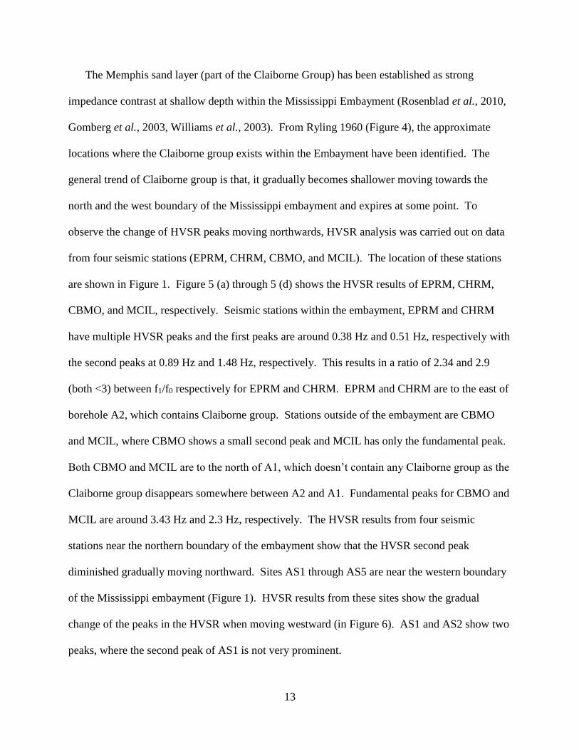
The Memphis sand layer (part of the Claiborne Group) has been established as strong

impedance contrast at shallow depth within the Mississippi Embayment (Rosenblad et al., 2010,

Gomberg et al., 2003, Williams et al., 2003). From Ryling 1960 (Figure 4), the approximate

locations where the Claiborne group exists within the Embayment have been identified. The

general trend of Claiborne group is that, it gradually becomes shallower moving towards the

north and the west boundary of the Mississippi embayment and expires at some point. To

observe the change of HVSR peaks moving northwards, HVSR analysis was carried out on data

from four seismic stations (EPRM, CHRM, CBMO, and MCIL). The location of these stations

are shown in Figure 1. Figure 5 (a) through 5 (d) shows the HVSR results of EPRM, CHRM,

CBMO, and MCIL, respectively. Seismic stations within the embayment, EPRM and CHRM

have multiple HVSR peaks and the first peaks are around 0.38 Hz and 0.51 Hz, respectively with

the second peaks at 0.89 Hz and 1.48 Hz, respectively. This results in a ratio of 2.34 and 2.9

(both <3) between f1/f0 respectively for EPRM and CHRM. EPRM and CHRM are to the east of

borehole A2, which contains Claiborne group. Stations outside of the embayment are CBMO

and MCIL, where CBMO shows a small second peak and MCIL has only the fundamental peak.

Both CBMO and MCIL are to the north of A1, which doesn’t contain any Claiborne group as the

Claiborne group disappears somewhere between A2 and A1. Fundamental peaks for CBMO and

MCIL are around 3.43 Hz and 2.3 Hz, respectively. The HVSR results from four seismic

stations near the northern boundary of the embayment show that the HVSR second peak

diminished gradually moving northward. Sites AS1 through AS5 are near the western boundary

of the Mississippi embayment (Figure 1). HVSR results from these sites show the gradual

change of the peaks in the HVSR when moving westward (in Figure 6). AS1 and AS2 show two

peaks, where the second peak of AS1 is not very prominent.

14

Figure 4. Himel, et al. (separate pdf file attached for clarity)

Figure 4. Himel, et al.

Figure 4: Generalized geologic cross section of the Mississippi embayment from boreholes

originally presented in Ryling (1960): (a) North-South cross section for boreholes A1 – A14 and

(b) East-West cross section for boreholes B1 – B7.

15

Fundamental peak of AS1 and AS2 are 0.36 Hz and 0.53 Hz, respectively. The f1/f0 ratio for

AS1 and AS2 are respectively 2.78 and 3.36. AS3, AS4, and AS5 sites have only fundamental

peaks at 0.39 Hz, 1.12 Hz, and 2.24 Hz, respectively. Thus, it could be inferred that the HVSR

second peak in the Mississippi embayment exists where shallow impedance contrast from

Memphis sand layer is present and disappears with the disappearance of the Memphis sand layer.

Figure 5: HVSR result of seismic stations EPRM, CHRM, CBMO, and MCIL.

16

Figure 6: HVSR results of the Additional Sites along the western edge of the Mississippi

Embayment.

Table 2 shows the second peak frequency and fundamental frequency along with the f1/f0

ratio for the 17 sites with HVSR second peak. The average of f1/f0 ratio of the 17 sites is found to

17

be 3.5 Hz with a sample standard deviation of 0.733 Hz. A hypothesis test on the population

mean of f1/f0 was carried out, where

Null hypothesis, H0: Population mean of f1/f0, 𝝁 = 3.0

Alternative hypothesis, H1: Population mean of f1/f0, 𝜇 ≠ 3.0

Now using the equation, 𝑡 = �̅�−𝜇𝑠

√𝑛⁄

Where, t=test statistics, �̅� =sample mean, 𝜇 =population mean, 𝑠 =sample standard

deviation, 𝑛 =number of samples. The test statistics, t was found to be 2.81, which is greater

than the critical value of a two tailed t distribution at 5% level of significance, tc=2.120. Thus,

the null hypothesis is rejected that the population mean is equal to 3.

Applying Students t test on the f1/f0 ratio, the lower and upper bound for population mean of

f1/f0 are found to be 3.124 Hz and 3.876 Hz, respectively at 95% confidence interval. This

indicates that there is 95% certainty that the population mean of f1/f0 will be between 3.124 Hz

and 3.876 Hz, indicating the ratios of the peaks is not three and likely not the result of odd

harmonics.

Table 2 Second peak frequency and fundamental frequency along with their ratio, for the sites

with HVSR second peak.

Site Type Name f0 (Hz) f1 (Hz) f1/f0

NEA Sites

Amagon 0.413 2.154 5.22

Marmaduke 0.312 0.933 2.99

Bay 0.272 1.072 3.94

Monette 0.271 1.077 3.97

Harrisburg 0.26 0.977 3.76

Manila 0.247 0.85 3.44

Marked Tree 0.238 1.024 4.30

18

Table 2 (Cont.)

Site Type Name f0 (Hz) f1 (Hz) f1/f0

Athelstan 0.238 0.739 3.11

Wynne 0.225 0.933 4.15

Palestine 0.218 0.928 4.26

Earle 0.211 0.643 3.05

Greasy Corner 0.207 0.559 2.70

Aubrey 0.186 0.617 3.32

AS AS1 0.36 1.001 2.78

AS2 0.53 1.78 3.36

Seismic Station EPRM 0.38 0.89 2.34

CHRM 0.51 1.48 2.90

5.0 Inversion Results at Manila, AR

The Manila site is located in the Mississippi County, Arkansas, which is geologically situated

in the lowlands. As per Dart 1995, the depth to bedrock for Manila is around 750 m, whereas the

CUSVM indicates a depth of 813 m (Ramírez‐Guzmán et al., 2012). The Memphis sand depth

at this site is at 83 m and around 200 m as per CUSVM and Ryling 1960, respectively. For shear

wave velocity profiling at this site, a combination of active source multi-channel analysis of

surface wave (MASW), passive source Microtremor array measurements (MAM) and horizontal

to vertical spectral ratio (HVSR) measurements were carried out. The active source MASW was

carried out using 24, 4.5 Hz geophone with 2 m spacing using both vertical (Rayleigh) and

horizontal (Love) geophones. A 4.5 kg hammer was used for the vertical and horizontal impact

to generate Rayleigh and Love wave, respectively. For ensuring high quality data and

minimizing near field effects, source offset of 5 m, 10 m, 20 m, and 40 m were used from the

first geophone of the array. At each source offset location, 10 vertical/horizontal impacts were

19

stacked to increase the signal to noise ratio. MAM measurements were made using circular

arrays of 50 m, 200 m, and 500 m diameter. Three component Nanometrics Trillium Compact

20 s broadband seismometers were used. In each array, one seismometer was placed at the

center of the array and nine uniformly distributed around the circumference. Ambient noise was

recorded for one hour for the 50 m and 200 m diameter arrays and for two hours for the 500 m

diameter array.

The Rayleigh and Love wave MASW data were processed using the multiple-source offset

technique combined with the Frequency Domain Beamformer (FDBF) method (Zywicki et al.,

1999, Cox et al., 2011). Rayleigh wave dispersion data from vertical component of ambient

noise, recorded from the circular arrays were processed using the High-Resolution Frequency

Wavenumber (HRFK) method (Capon 1969) and the Modified Spatial Auto-Correlation

(MSPAC) method (Bettig et al., 2001). Love wave data from MAM were also processed using

the HRFK processing. The individual curves from each method and arrays (MAM) were first

cleared of outlying points. Then a composite dispersion curve was produced combining the

dispersion curves from each method (Park et al., 1999, Foti et al., 2014). This composite

dispersion curve along with the HVSR peak were used to make a joint inversion in the Geopsy

software package Dinver. Details of the dispersion processing could be found in Wood et al.,

2018.

The f0 and f1 HVSR peaks for the Manila site are respectively 0.247 Hz and 0.85 Hz with a

f1/f0 ratio of 3.44 (>3.0). From Ryling 1960, two borehole B5 and B6 are located close to the

Manila site, respectively 2.65 km to the east and 4.2 km to the north-east of Manila. From the

borehole logs, it was estimated that B5 and B6 has the Memphis sand layer starting from 200 m

20

and 220 m, respectively. Utilizing this borehole information and CUSVM, a preliminary idea

about Memphis sand depth at the Manila site was estimated to be around 80-200 m.

Figure 7 (a) through (c) illustrates three separate shear wave velocity models for Manila.

The 83 m model, shown in Figure 7 (a) is generated by Wood et al. 2018 by joint inversion of

the dispersion data and HVSR fundamental peak. For this model, layer parameterization was

created using CUSVM (Ramírez‐Guzmán et al. 2012) geologic unit boundaries and a subset of

layers to allow varying layer thickness. Vs, and Vp ranges for the parameterization for each layer

is based on Lin et al., 2014, Romero and Rix 2005, Rosenblad et al., 2010, Ramírez‐Guzmán et

al., 2012, and Woolery et al., 2016. The model shown in Figure 7 (a) demonstrates the potential

Memphis sand layer to start from 83 m, which is coherent with the CUSVM Memphis sand

depth at this location.

To resolve the Memphis sand depth more accurately in the VS profile, two more Vs models

were generated in this paper. For these models, the inversions were carried out in two phases. In

the first phase, instead of the fundamental frequency, the HVSR second peak frequency was used

to constrain the Memphis sand depth. The same parameterization used for the 83 m model was

used down to the predicted Memphis sand depth. Dispersion data along with the HVSR second

peak was inverted. In the second phase, the resulting Vs profile from the first phase was used to

constrain the parameterization down to the Memphis sand depth found in the first phase. The

remainder of the parameters were same as Wood et al., 2018. As the second phase is a full scale

inversion down to the bedrock, the fundamental peak was used along with the dispersion data.

For the 131 m model, the first phase inversion was conducted using the 83 m model

parameterization down to 200 m (preliminary estimation of Memphis sand depth) and using the

HVSR second peak at 0.85 Hz. This resulted in demonstrating the Memphis sand depth around

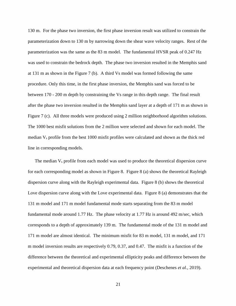
21

130 m. For the phase two inversion, the first phase inversion result was utilized to constrain the

parameterization down to 130 m by narrowing down the shear wave velocity ranges. Rest of the

parameterization was the same as the 83 m model. The fundamental HVSR peak of 0.247 Hz

was used to constrain the bedrock depth. The phase two inversion resulted in the Memphis sand

at 131 m as shown in the Figure 7 (b). A third Vs model was formed following the same

procedure. Only this time, in the first phase inversion, the Memphis sand was forced to be

between 170 - 200 m depth by constraining the Vs range in this depth range. The final result

after the phase two inversion resulted in the Memphis sand layer at a depth of 171 m as shown in

Figure 7 (c). All three models were produced using 2 million neighborhood algorithm solutions.

The 1000 best misfit solutions from the 2 million were selected and shown for each model. The

median Vs profile from the best 1000 misfit profiles were calculated and shown as the thick red

line in corresponding models.

The median Vs profile from each model was used to produce the theoretical dispersion curve

for each corresponding model as shown in Figure 8. Figure 8 (a) shows the theoretical Rayleigh

dispersion curve along with the Rayleigh experimental data. Figure 8 (b) shows the theoretical

Love dispersion curve along with the Love experimental data. Figure 8 (a) demonstrates that the

131 m model and 171 m model fundamental mode starts separating from the 83 m model

fundamental mode around 1.77 Hz. The phase velocity at 1.77 Hz is around 492 m/sec, which

corresponds to a depth of approximately 139 m. The fundamental mode of the 131 m model and

171 m model are almost identical. The minimum misfit for 83 m model, 131 m model, and 171

m model inversion results are respectively 0.79, 0.37, and 0.47. The misfit is a function of the

difference between the theoretical and experimental ellipticity peaks and difference between the

experimental and theoretical dispersion data at each frequency point (Deschenes et al., 2019).

22

Figure 7: Median Vs profiles of the 83 m model, 131 m model and 171 m model along with the

1000 Vs best profiles are shown. For each model, the estimated Memphis sand depth is shown

with the thick black line. Reference Vs profiles of Lin et al., 2014 for different soil types are

provided for comparison

The misfit values are dependent on the quality and quantity of dispersion data and the

complexity of the geology (Teague et al., 2017). Along with the quantitative misfits, visual fit

quality was also inspected. The minimum misfit of the 83 m model is highest among all three

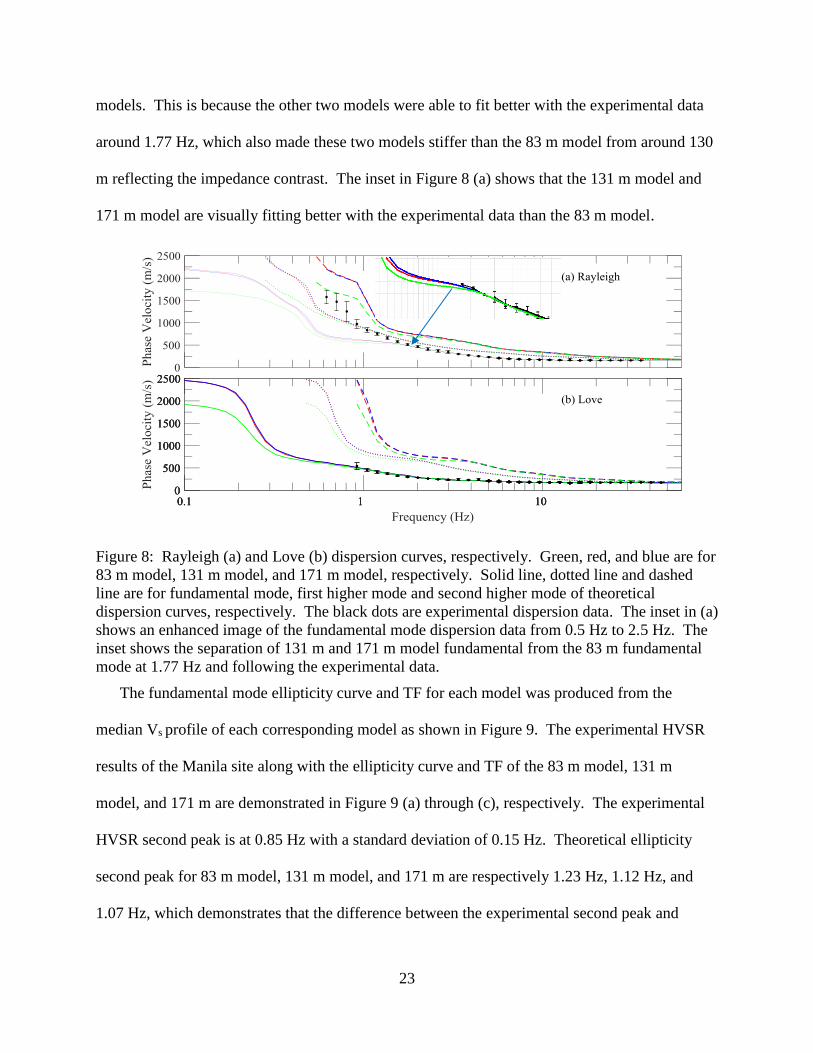
23

models. This is because the other two models were able to fit better with the experimental data

around 1.77 Hz, which also made these two models stiffer than the 83 m model from around 130

m reflecting the impedance contrast. The inset in Figure 8 (a) shows that the 131 m model and

171 m model are visually fitting better with the experimental data than the 83 m model.

Figure 8: Rayleigh (a) and Love (b) dispersion curves, respectively. Green, red, and blue are for

83 m model, 131 m model, and 171 m model, respectively. Solid line, dotted line and dashed

line are for fundamental mode, first higher mode and second higher mode of theoretical

dispersion curves, respectively. The black dots are experimental dispersion data. The inset in (a)

shows an enhanced image of the fundamental mode dispersion data from 0.5 Hz to 2.5 Hz. The

inset shows the separation of 131 m and 171 m model fundamental from the 83 m fundamental

mode at 1.77 Hz and following the experimental data.

The fundamental mode ellipticity curve and TF for each model was produced from the

median Vs profile of each corresponding model as shown in Figure 9. The experimental HVSR

results of the Manila site along with the ellipticity curve and TF of the 83 m model, 131 m

model, and 171 m are demonstrated in Figure 9 (a) through (c), respectively. The experimental

HVSR second peak is at 0.85 Hz with a standard deviation of 0.15 Hz. Theoretical ellipticity

second peak for 83 m model, 131 m model, and 171 m are respectively 1.23 Hz, 1.12 Hz, and

1.07 Hz, which demonstrates that the difference between the experimental second peak and

24

theoretical ellipticity second peak are decreasing gradually with increasing Memphis sand depth.

The resonance frequency from the TF of 83 m model, 131 m model, and 171 m are respectively

0.2333 Hz, 0.2457 Hz, and 0.2436 Hz. The 83 m model, 131 m model, and 171 m model TF

resonance frequency have 5.5%, 0.52%, and 1.39% difference with the HVSR fundamental

frequency.

Between 131 m model and 171 m model, the former has the lowest minimum misfit,

indicating a better fit with the experimental data. The 131 m model was not forced in the first

phase of the inversion to resolve the impedance contrast depth, rather it was allowed to search

for the best fit. The 131 m model demonstrates the lowest difference between its TF resonance

frequency and HVSR fundamental frequency. The approach to generate the 131 m model is

practically more suitable as it only needs a tentative idea of the impedance contrast depth but still

gives a better result considering the shear wave transfer function.

25

Figure 9: Shear wave transfer function and theoretical ellipticity curve for each model along with

the Manila HVSR respectively for the 83 m model (a), 131 m model (b), and 171 m model (c).

26

6.0 Conclusion:

The horizontal to vertical spectral ratio method was used to estimate the resonance frequency

at 15 sites in North East Arkansas. The HVSR results of thirteen sites showed prominent second

peak in addition to the fundamental HVSR peak. Shear wave transfer functions were compared

for select sites with the HVSR second peaks which indicated poor agreement between the second

HVSR peak and the second peak in the shear transfer function for 10 of the 13 sites with second

HVSR peaks. In addition, the ratio of f1/f0 was shown to be greater than 3 at a majority of the

sites reducing the likelihood that an odd harmonic is causing the second HVSR peak. To relate

the HVSR results with the Mississippi embayment geology, four seismic stations and an

additional five HVSR sites were selected near the northern and western borders of the

embayment. The additional HVSR results showed that the HVSR second peak disappeared

gradually with the gradual diminishing of Memphis sand layer indicating the second HVSR peak

is only present in areas where the Memphis sand exists.

The HVSR second peak was then used along with the fundamental peak and dispersion data

to conduct a joint inversion in two phases for a site in Manila, AR. The two VS models

generated in this procedure demonstrates the Memphis sand depth at 131 m and 171 m provides

a better fit to the experimental data and borehole information than the estimated depth provided

by the CUSVM at 83 meters. This demonstrates the usefulness of including the second HVSR

peak in the joint inversion for sites in the Mississippi Embayment.

Applying the new approach of VS profiling utilizing HVSR second peak for the rest of the

NEA sites could be a topic of the future study as the experimental dispersion data for all fifteen

North East Arkansas sites are available from Wood et al., 2018.

27

References:

Ari, H. and Tokimatsu, K., 2005. S-Wave Velocity Profiling by Joint Inversion of

Microtremor Dispersion Curve and Horizontal-to-Vertical (H/V) Spectrum, Bull. Seism.

Soc. Am 95(5), 1766–1778, DOI: 10.1785/0120040243.

Bailey, J., P., 2008. Development of shear wave velocity profiles in the deep sediments of

the Mississippi Embayment using surface wave and spectral ratio methods, MS Thesis,

University of Missouri-Columbia, Columbia.

Bettig, B., Bard, P.Y., Scherbaum, F., Riepl, J., Cotton, F., Cornou, C., and Hatzfield, D.,

2001. Analysis of dense array noise measurements using the modified spatial auto

correlation method (SPAC): application to the Grenoble area, Bollettino de Geofisica

Teoria e Applicata 42(3-4), 281-304.

Bodin, P., Smith, K., Horton, S., Hwang, H., 2001. Microtremor observations of deep

sediment resonance in metropolitan Memphis, Tennessee, Engineering Geology 62, 159-

168.

Bonnefoy-Claudet, S., Cornou, C., Bard, P.-Y., Cotton, F., Moczo, P., Kristek, J. & Fah, D.,

2006. H/V ratio: a tool for site effects evaluation. Results from 1-D noise simulations,

Geophys. J. Int. 167, 827–837.

Bonnefoy-Claudet, S., Kohler, A., Cornou, C., Wathelet, M., Bard, P.-Y., 2008. Effects of

love waves on Microtremor H/V ratio, Bull. Seism. Soc. Am 98(1), 288-300.

Brahana, J.V., Parks, W. S., and Gaydos, M. W., 1987. Quality of Water from Freshwater

Aquifers and Principal Well Fields in the Memphis Area, Tennessee. USGS Water-

Resources Investigations Report 87-4052.

Capon, J., 1969. High Resolution Frequency-Wavenumber Spectrum Analysis, Proceedings

of IEEE 57(8), 1408–1418.

Carpenter, N. S., Wang, Z., Woolery, E. W., Rong, M., 2018. Estimating site response with

recordings from deep boreholes and HVSR: examples from the Mississippi embayment

of the Central United States, Bull. Seism. Soc. Am 108(3A), 1199-1209.

Cox, B.R. and Wood, C.M., 2011. Surface Wave Benchmarking Exercise: Methodologies,

Results and Uncertainties, in Proceedings, in Proceedings, GeoRisk 2011, June 26-28,

2011, Atlanta, GA, USA.

Cramer, C. H., 2006. Quantifying the uncertainty in site amplification modeling and its

effects on site-specific seismic-hazard estimation in the upper Mississippi embayment

and adjacent areas. Bull. Seism. Soc. Am 96(6), 2008 - 2020.

Cushing, E.M., Boswell, E.H., and Hosman, R.L, 1964. General geology of the Mississippi

Embayment, Water Resources of Mississippi Embayment, U.S. Geological Survey

Professional Paper 448-B.

Dart, R.L., 1995. Maps of upper Mississippi Embayment Paleozoic and Precambrian Rocks,

U.S. Geologic Survey, Miscellaneous. Field Study Map, MF-2284, 235 - 249.

28

Deschenes, M. R., Wood, C. M., Himel, A. K., Baker, E., 2019. Development of deep shear

wave velocity profiles in Mississippi Embayment. Earthquake Spectra (in review).

DiGiulio, G., Savvaidis, A., Ohrnberger, M., Wathelet, M., Cornou, C., Knapmeyer-Endrun,

B., Renalier, F., Theodoulidis, N. and Bard, P.Y., 2012. Exploring the model space and

ranking a best class of models in surface-wave dispersion inversion: Application at

European strong-motion sites, Geophysics 77(3), B147–B166.

Dunand, F., et al. 2004. Utilisation du bruit de fond pour l’analyse des dommages des

baˆtiments de Boumerdes suite au se´isme du 21 mai 2003, Mem. Serv. Geol. Alger. 12,

177– 191.

Dunkin, J.W., 1965. Computation of modal solutions in layered, elastic media at high

frequencies, Bull. Seism. Soc. 55, 335–358.

Ervin, C. P., and McGinnis, L. D., 1975. Reelfoot Rift: Reactivated precursor to the

Mississippi Embayment, Geol. Soc. Am. Bull. 86, 1287 – 1295.

Farrugia, D., Paolucci, E., D’Amico, S., Galea, P., 2016. Inversion of surface wave data for

subsurface shear wave velocity profiles characterized by a thick buried low-velocity

layer, Geophysical Journal International, 206, 1221-1231.

Field, E., and Jacob, K., 1993. The theoretical response of sedimentary layers to ambient

seismic noise, Geophys. Res. Lett. 20, 2925–2928.

Foti, S., Lai, C., Rix, G., and Strobbia, C., 2014. Surface Wave Methods for Near-Surface

Site Characterization, 1st edition, CRC Press, Boca Raton, FL, 487 pp.

Goetz, R., P., 2009. Study of the horizontal-to-vertical spectral ratio (HVSR) method for

characterization of deep soils in the Mississippi Embayment, MS Thesis, University of

Missouri-Columbia, Columbia.

Gomberg, J., Waldron, B., Schweig, E., Hwang, H., Webbers, A., Van Arsdale, R., et al.,

2003. Lithology and shear-wave velocity in Memphis, Tennessee. Bull. Seism. Soc. 93

(3), 986–997.

Ginzburg, A., Mooney, W. D., Walter, A. D., Lutter, W. J., and Healy, J.H., 1983. Deep

structure of the northern Mississippi Embayment, Bull. Am. Assoc. Petr. Geol. 67, 2031-

2046.

Guéguen, P., Chatelain, J.-L., Guillier, B., and Yepes, H., and Egred, J., 1998. Site effect and

damage distribution in Pujili (Ecuador) after the 28 March 1996 earthquake, Soil Dyn.

Earthq. Eng. 17, 329–334.

Guéguen, P., Chatelain, J.-L., Guillier, B., and Yepes, H., 2000. An indication of the soil

topmost layer response in Quito (Ecuador) using HVSR spectral ratio, Soil Dyn. Earthq.

Eng. 19, 127–133.

Guillier, B., Chatelain, J.-L., Hellel, M., Machane, D., Mezouer, N., Ben Salem, R., 2005.

Smooth bumps in H/V curves over a broad area from single-station ambient noise

recordings are meaningful and reveal the importance of Q in array processing: The

Boumerdes (Algeria) case, Geophysical Research Letters 32, L24306.

29

Guo, Z., Aydin, A., Kuszmaul, J. S., 2014. Microtremor recordings in Northern Mississippi,

Engineering Geology 179, 146-157.

Guo, Z., Aydin, A., 2016. A modified HVSR method to evaluate site effect in Northern

Mississippi considering ocean wave climate, Engineering Geology 200, 104-113.

Hashash, Y., Phillips, C., and Groholski, D., 2010. Recent advances in non-linear site

response analysis, Paper No. OSP 4, in Proceedings, 5th International Conference on

Recent Advances in Geotechnical Earthquake Engineering and Soil Dynamics, 24-29

May, 2010, San Diego, California, USA.

Haskell, N. A., 1953. The dispersion of surface waves on multilayered media, Bull. Seism.

Soc. 43, 17–34.

Incorporated Research Institutions for Seismology (IRIS), 2018. Time series data Web page

for downloading seismic station data, available at

http://ds.iris.edu/ds/nodes/dmc/data/types/waveform-data/ (last accessed July, 2018)

Konno, K., Ohmachi, T., 1998. Ground motion characteristics estimate from spectral ratio

between horizontal and vertical components of microtremor, Bull. Seism. Soc. Am. 88 (1),

228-241.

Lachet, C., D. Hatzfeld, P.-Y. Bard, N. Theodulidis, C. Papaioannou and A. Savvaidis, 1996.

Site effects and microzonation in the city of Thessaloniki (Greece): comparison of

different approaches, Bull. Seism. Soc. Am. 86, 1692-1703.

Lin, Y. C., Joh, S. H, and Stokoe, K. H., 2014. Analyst J: Analysis of the UTexas 1 Surface

Wave Dataset Using the SASW Methodology, Geo-Congress 2014 Technical Papers:

Geo-Characterization and Modeling for Sustainability. GSP 234. 2014.

Macau, A., Benjumea, B., Gabàs, A. et al., 2015. The effect of shallow Quaternary deposits

on the shape of the H/V spectral ratio, Surv. Geophys. 36, 185-208.

https://doi.org/10.1007/s10712-014-9305-z

Mento, D.J., Ervin, C.P., McGinnis, L.D., 1986. Periodic energy release in the New Madrid

seismic zone, Bull. Seism. Soc. Am. 76, 1001-1009.

Nakamura, Y., 1989. A method for dynamic characteristics of subsurface using microtremors

on the ground surface, Quick Report of Railway Technical Research Institute, 30, 25-33.

Nakamura, Y., 2008. On the H/V spectrum, Paper No. 07-0033, 14th World Conference on

Earthquake Engineering, 12–17 October, 2008, Beijing, China.

Ng, K. W., Chang, T. S., Hwang, H., 1989. Subsurface conditions of Memphis and Shelby

County. Technical report NCEER-89-0021, National Center for Earthquake Research,

State University of New York at Buffalo, Buffalo, NY.

Park, C. B., Miller, R. D. & Xia, J., 1999. Multichannel analysis of surface waves,

Geophysics 64, 800-880.

30

Ramírez‐Guzmán, L., O., Boyd, S., Hartzell, R., Williams, 2012. Seismic velocity model of

the central United States (Version 1): Description and simulation of the 18 April 2008

Mt. Carmel, Illinois, Earthquake, Bull. Seism. Soc. Am. 102, 2622-2645.

Romero, S.M., Rix, G.J., 2005. Ground Motion Amplification of Soil in the Upper

Mississippi Embayment. GIT-CEE/GEO-01-1, National Science Foundation Mid

America Center, Atlanta.

Rosenblad, B., 2008. Deep shear wave velocity profiles of Mississippi Embayment sediments

determined from surface wave measurements, U.S. Geol. Surv. Final Tech. Rept., USGS

NEHRP Award No. 06HQGR0131, 23 pp.

Rosenblad, B., Bailey, J., Csontos, R. and Van Arsdale, R., 2010. Shear Wave Velocities of

Mississippi Embayment Soils from Low Frequency Surface Wave Measurements, Soil

Dynamics and Earthquake Engineering 30, 691 – 701.

Rosenblad, B., Goetz, R., 2010. Study of the H/V spectral ratio method for determining

average shear wave velocities in the Mississippi Embayment, Engineering Geology 112,

13-20.

Ryling, R. W., 1960. Ground water potential of Mississippi County, Arkansas, Water

Resources Circular, Arkansas Geological Survey, 13-16.

Scherbaum, F., Hinzen, K. G., and Ohrnberger, M., 2003. Determination of shallow shear

wave velocity profiles in the Cologne/Germany area using ambient vibrations,

Geophysical Journal International 152, 597–612.

Schwalb, H. R., 1971. The northern Mississippi Embayment- A latent Paleozoic oil province,

in Proceedings, Symposium on Future Petroleum Potential of NPC Region 9 (Illinois

Basin Cincinnati Arch, and Northern Part of Mississippi Embayment), 11-12 March,

1971, Champaign, Illinois, USA.

SESAME European project (2004) Guidelines for the Implementation of the H/V Spectral

Ratio Technique on Ambient Vibrations: Measurements, Processing and Interpretation.

Deliverable D23.12.

Teague, D., Cox, B., Bradley, B. and Wotherspoon, L.M. (2017) Development of Deep Shear

Wave Velocity Profiles with Estimates of Uncertainty in the Complex Inter-Bedded

Geology of Christchurch, in review.

Teague, D. P., Cox, B. R., Rathje, E. M., 2018. Measured vs. predicted site response at the

Garner valley downhole array considering shear wave velocity uncertainty from borehole

and surface wave methods, Soil Dynamics and Earthquake Engineering 113, 339-355

Thomson, W. T., 1950. Transmission of elastic waves through a stratified solid medium,

Journal of Applied Physics 21, 89–93.

Van Arsdale, R.B., TenBrink, R.K., 2000. Late Cretaceous and Cenozoic Geology of the

New Madrid Seismic Zone, Bull. Seism. Soc. Am. 90, 345–356.

Wathelet, M., 2008. An improved neighborhood algorithm: parameter conditions and

dynamic scaling, Geophysical Research Letters 35, L09301.

31

Williams, R. A., Wood, S., Stephenson, W. J., et al., 2003. Surface seismic

refraction/reflection measurement determinations of potential site resonances and the

areal uniformity of NEHRP site class D in Memphis, Tennessee. Earthquake Spectra 19

(1), 159-89.

Wood, C. M., Baker, E., Deschenes, M., Himel, A. K., 2018. Deep shear wave velocity

profiling in Northeastern Arkansas, TRC 1603, Arkansas Department of Transportation.

Wotherspoon, L.M., Munro, J., Bradley, B.A., Wood, C.M., Thompson, E., Deschenes, M.,

Cox, B. (2018). Site period characteristics across the Canterbury region of New Zealand,

GEESD conference, Austin TX, June 2018.

Woolery, E. W., Wang, Z., Carpenter, N. S., Street, R., Brengman, C., 2016. The Central

United States Seismic Observatory: Site Characterization, Instrumentation, and

Recordings. Seismological Research Letters 87 (1), 215–228.

https://doi.org/10.1785/0220150169

Zaslavsky, Y., et al., 2007. Use of ambient vibration measurements for reconstruction of

subsurface structure along three profiles in the Zevulun Plain, Report No 571/240/07, The

Geophysical institute of Israel.

Zywicki, D.J., 1999. Advanced signal processing methods applied to engineering analysis of

seismic surface waves, Ph.D. Dissertation, School of Civil and Environmental

Engineering, Georgia Institute of Technology, Atlanta, GA.