utmis.org.loopiadns.comutmis.org.loopiadns.com/...fatigue_stockholm_08.pdf · • the stress...
TRANSCRIPT
© 2008 Grzegorz Glinka. All rights reserved. 1
Fatigue Design of Welded Structures Fatigue Design of Welded Structures --
Physical Physical Modeling vs. Empirical RulesModeling vs. Empirical Rules
G. G. GlinkaGlinka, Ph.D., D.Sc., Ph.D., D.Sc.
University of Waterloo,Department of Mechanical and Mechatronics
Engineering,
200 University Ave. W, Waterloo,
Ontario, Canada N2L 3G1
Phone: 1-519-888 4567 ext. 33339
e-mail: [email protected]
Stockholm, 21-22, October 2008
© 2008 Grzegorz Glinka. All rights reserved. 2
ContentsContents1) Brief review of American and European rules concerning static
strength analysis of weldments,
•
The structural nature of welded joints•
Static strength of weldments•
The customary US/American method (AWS)•
The IIW/ISO method•
Simple welded joint analysis•
Example
2) Outline of contemporary fatigue analysis methods –
similarities, differences and limitations,
•
the classical nominal stress method (S -
N), •
the local strain-life approach,(ε
– N)•
the fracture mechanics approach (da/dN
–
ΔK),
3) Load/stress histories•
methods of assembling characteristic load/stress histories, •
the rainflow counting method – live example, •
extraction of load/stress cycles from the frequency domain data,
© 2008 Grzegorz Glinka. All rights reserved. 3
4) Loads and stresses in fatigue•
the stress concentration in weldments, •
the nominal stress, the hot spot stress and the peak stress at the weld toe,•
the use of the Finite Element method for the stress analysis in weldments,•
residual stresses;
5) The strain-life (ε
–
N)
approach to fatigue life assessment of weldments•
material properties and their scatter,•
linear elastic stress distributions in weldments,•
the actual elastic-plastic stress-strain response at the weld toe, •
the multiaxial Neuber and the ESED method (uniaxial and multi-axial), •
superposition of applied and residual stresses,•
fatigue damage accumulation,•
deterministic fatigue life prediction – the effect of the weld geometry and residual stresses,
•
quantification of the scatter of the load, weld geometry and material properties on the on the scatter of the predicted life,
•
application of the Monte-Carlo simulation method for the estimation of the fatigue reliability;
© 2008 Grzegorz Glinka. All rights reserved. 4
6) The Fracture Mechanics approach• basics of fatigue crack growth analysis• stress intensity factors for cracks in weldments,• the weight function approach – 2-D and 3-D solutions,• the residual stress effect,• modeling of the fatigue crack growth of irregular planar cracks, • quantification of the scatter and the Monte Carlo simulation),
7) Simple methods for improvement of fatigue performance of welded structures• decrease of the stress concentration, • elimination of the local bending effect, • modification of the stress path, • optimization of the global geometry of a welded structure, • introduction of favorable residual stresses• live examples
8) Recent developments in the fatigue crack growth analysis • The UniGrow fatigue crack growth model for spectrum loading

© 2008 Grzegorz Glinka. All rights reserved. 5
1.
Bannantine, J., Corner, Handrock, Fundamentals of Metal Fatigue Analysis, Prentice-Hall, 1990.... (complete, correct, up to date)
2. Dowling, N., Mechanical Behaviour of Materials, Prentice Hall, 1999...
( middle chapters are a great overview of most recent views on fatigue analysis)
3. M. Janssen, J. Zudeima, R.J.H. Wanhill, Fracture Mechanics, VSSD, The Netherlands, 2006 (understandable, rigorous, mechanics perspective)
4. Stephens, R.I., Fatemi, A., Stephens, A.A., Fuchs, H.O., Metal Fatigue in Engineering, John Wiley, 2001.... (good general reference, well done)
5. Radaj, D., Design and Analysis of Fatigue Resistant Structures,
Halsted
Press, 1990..... (Complete, civil engineering analysis perspective)
6.Suresh, S., Fatigue of Materials,
Cambridge University Press, 1998.... (Encyclopedic, up to date, fundamental metallurgical perspective)
7. Anderson, T.L., Fracture Mechanics-Fundamentals and Applications, CRC Press, Boca Raton, 1995
8. Collins, J. A., Failure of Materials in Mechanical Design, John Wiley & Sons, New York, 1993
9. Broek, D., Elementary Engineering Fracture Mechanics, Martinus
Nijhoff, The Hague, 1982
10. Hertzberg, R.W., Deformation and Fracture Mechanics of Engineering
Materials, John Wiley, New York, 1989.
BibliographyBibliography

© 2008 Grzegorz Glinka. All rights reserved. 6
11. K. Iida and T. Uemura, “Stress Concentration Factor Formulas Widely Used in Japan”, Document IIW XIII-1530-94, The International Welding Institute, 1994.
12. Bahram
Farhmand, G. Bockrath
and J. Glassco, Fatigue and Fracture Mechanics of High Risk Parts, Chapman @Hall, 1997
13. Sandor, R.J., Principles of Fracture Mechanics,
Prentice Hall, Upper Saddle River, 2002.
14. Socie, D.F., and Marquis, G.B., Multiaxial
Fatigue, Society of Automotive Engineers, Inc., Warrendale, PA, 2000.
15. Serensen, S.V., Kogayev, V.P., Shneyderovich, R.M., Nesushchaya
Sposobnost
i Raschyoty
Detaley
Machin
na
Prochnost, Mashinostroyene, Moskva, 1975 (in Russian)
16. Machutov, N.A., Resistance of Structural Elements Against Brittle Fracture, Mashinostroenye, Moscow, 1973 (in Russian).
17. Cherepanov, G.P., Mechanika
chrupkovo
razrusheniya, Nauka, Moscow, 1974 (in Rusian).
18. Bathias, C., and Bailon, J.-P., La Fatigue des Materiaux
et des Structures, Maloine
S.A. Editeur, Paris, 1980 (in French).
19. Haibach, E., Betriebsfestigkeit, VDI Verlag, Dusseldorf, 1989 (in German).
20. Barsom, J.M, and Rolfe, S.T., Fracture and Fatigue Control in Structures, Prentice Hall, New Jersey, 1987.
21. Courtney, T.H., Mechanical Behavior
of Materials, McGraw Hill, New York, 1990.
Bibliography Bibliography (continued)(continued)

© 2008 Grzegorz Glinka. All rights reserved. 7
22. Collins, J.C., Mechanical Design of Machine Elements and Machines, John Wiley & Sons, New York, 2003.
23. Shigley, J.E., and Mischke, C.R., Mechanical Engineering Design, McGraw-Hill, New York, 2001
24. Juvinal, R.C., and Marshek, K.M., Fundamentals of Machine Components Design, John Wiley & Sons, New York, 2000.
25. Norton, R.L., Machine Design –
An Integrated Approach, Prentice Hall, New Jersey, 2000
26. Hamrock, B.J., Jacobson, Bo and Schmid, S.R., Fundamentals of Machine Elements, McGraw-
Hill, Boston, 1999.
27. Orthwein, W., Machine Component Design, West Publishing Company, New York, 1990.
28. J.-L. Fayard, A. Bignonnet
and K. Dang Van, “Fatigue Design Criterion for Welded Structures”, Fatigue and Fracture of Engineering Materials and Structures, vol. 19, No.6, 19996, pp723-729.
29. V.A. Ryakhin
and G.N. Moshkarev, Durability and Stability of Welded Structures in Earth Moving Machinery”, Mashinostroenie, Moscow, 1984 (in Russian)
30. 7. V. I. Trufyakov
(editor), The Strength of Welded Joints under Cyclic Loading, Naukova
Dumka, Kiev, 1990 (in Russian).
31. J.Y. Young and F.V. Lawrence, ”Analytical and Graphical Aids for the Fatigue Design of Weldments”, Fracture and Fatigue of Engineering Materials and Structures, vol. 8, No.3, 1985, pp. 223-241.
Bibliography Bibliography (continued)(continued)
© 2008 Grzegorz Glinka. All rights reserved. 8
32. S.V. Petinov, Principles of Engineering Fatigue Analyses of Ship Structures, Sudostroyenie, Leningrad, 1990 (in Russian and in English)
33. C.C. Monahan, Early Fatigue Cracks Growth at Welds, Computational Mechanics Publications, Southampton UK, 1995.
34. Y. Murakami et. al, (editor), Stress Intensity Factors Handbook,
Pergamon
Press, Oxford, 1987
35. O.W. Blodgett, Design of Welded Structures, The James F. Lincoln Arc Welding Foundation, Cleveland, Ohio, 1966
36. A. Almar-Naess, Fatigue Handbook –
Offshore Steel Structures, Tapir Publishers, Trondheim, Norway, 1985
37. E. Niemi, Structural Stress Approach To Fatigue Analysis Of Welded Components,
The International Institute of Welding, Doc. XIII-WG3-06-99, 1999
38. D. Pingsha, A Structural Stress Definition and Numerical Implementation for Fatigue Analysis of Welded Joints, International Journal of Fatigue, vol. 23, 2001, p. 865-876
39. R.E. Little andJ.C. Ekvall, Statistical Analysis of Fatigue Data, ASTM STP 744, 1981
40. J.D. Burke and F.V. Lawrence, The Effect of Residual Stresses on Fatigue Life, FCP Report no. 29, University of Illinois, College of Engineering, 1978
41. J.G. Hicks, Welded Joint Design, Abington Publishing, UK, 1997-edition 2 and 1999-edition 3.
Bibliography Bibliography (continued)(continued)

© 2008 Grzegorz Glinka. All rights reserved. 9
Technical Report on Fatigue Properties
-
SAE J1099, SAE Book of Standards, 1992, SAE, p. 3.76
Standard Practices for Cycle Counting in Fatigue Analysis, ASTM Standard E 1049 -
85, ASTM Book of Standards, vol. 03.01, 1994, p. 789
Standard Recommended Practice for Contant-Amplitude Low-Cycle Fatigue Testing, ASTM Standard E 606 -
80, ASTM Book of Standards, vol. 03.01, 1994, p. 609
Standard Practice for Stastical
Analysis of Linearized
Stress-Life (S-N) and Strain-Life (ε-N) Fatigue Data, ASTM Standard E 739 -
91, ASTM Book of Standards, vol. 03.01, 1994, p. 682
Standard Test Method for Measurement of Fatigue Crack Growth Rates, ASTM Standard E 647 -
91, ASTM Book of Standards, vol. 03.01, 1996.
Relevant StandardsRelevant Standards
© 2008 Grzegorz Glinka. All rights reserved. 10
Relevant Relevant wwebsitesebsites
--
FatigueFatiguehttp://www.tech.plym.ac.uk/sme/Interactive_Resources/tutorials/FractureMechanics/index.html
(**Good basic course notes and tutorials on Fracture Mechanics)
http://www.sv.vt.edu/classes/MSE2094_NoteBook/97ClassProj/anal/kelly/fatigue.html#life
(*good overview notes)
http://www.engr.sjsu.edu/WofMatE/FailureAnaly.htm
(*Failure of Materials, examples)
http://www.sv.vt.edu/classes/MSE2094_NoteBook/97ClassProj/exper/ballard/www/ballard.html
(*General notes on fatigue)
http://highered.mcgraw-hill.com/sites/0072520361/student_view0/machine_design_tutorials.html
(*Tutorials on Strength theories, Stress concentration factors and Pressure vessel design)
http://emat.eng.hmc.edu/Calculators/shaft/shaft_design.htm
(*Calculator for shaft design, static and fatigue)
http://pergatory.mit.edu/2.75/software_tools/software_tools.html
(*Excel Files, stress concentration factors for shafts and design of shafts)
http://www.roymech.co.uk/Useful_Tables/Drive/Shaft_design.html
(*Interesting notes on shaft design and Tables)
http://www.fatiguecalculator.com/
(Stress concentration factors, fatigue methods)
http://www.saffd.com/
(*Fatigue software, manual and theory of fatigue methods)

© 2008 Grzegorz Glinka. All rights reserved. 11
Relevant Websites Relevant Websites ––
Fracture MechanicsFracture Mechanicshttp://www.tech.plym.ac.uk/sme/Interactive_Resources/tutorials/FractureMechanics/index.html
(**Good basic course notes and tutorials on Fracture Mechanics)
http://simscience.org/cracks/advanced/cracks1.html
(*Cracking of dams, history of FM, animations)
http://www.mech.uwa.edu.au/DANotes/fracture/LEFM/LEFM.html
(**Good notes on FM from Australia)
http://www.modares.ac.ir/eng/mmirzaei/
(**Good complete notes on Fracture Mechanics)
http://www.efunda.com/formulae/solid_mechanics/fracture_mechanics/fm_intro.cfm
(**Concise notes/explanations of basics of FM)
http://en.wikipedia.org/wiki/Fracture_mechanics
(* Fracture Mechanics –
the Wikipedia
way)
http://www.engin.brown.edu/courses/En222/Notes/Fracturemechs/Fracturemechs.htm
(**Plastic, brittle, fatigue fractures –
notes)
http://wwwold.ccc.commnet.edu/lta/lta4/index.pdf#search=%22Calculation%20of%20Stress%20Intensity%2
0Factors%22
(**NASA practical use of Fracture Mechanics –
good examples)
http://mysopromat.ru/uchebnye_kursy/mehanika_razrusheniya/spravochnye_dannye/funktsii_dlya_raschet
a_kin/
(Catalogue of SIF)
© 2008 Grzegorz Glinka. All rights reserved. 12
1) Brief review of American and European 1) Brief review of American and European rules concerning static strength analysis rules concerning static strength analysis of of weldmentsweldments,,
•
The structural nature of welded joints•
Static strength of weldments
•
The customary US/American method (AWS)•
The IIW/ISO method
•
Simple welded joint analysis•
Example
© 2008 Grzegorz Glinka. All rights reserved. 13
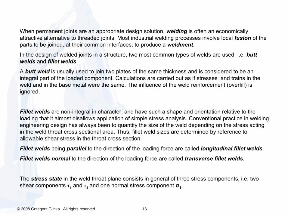
When permanent joints are an appropriate design solution, welding
is often an economically attractive alternative to threaded joints. Most industrial welding processes involve local fusion
of the parts to be joined, at their common interfaces, to produce a weldment.
In the design of welded joints in a structure, two most common types of welds are used, i.e. butt welds
and fillet welds.
A butt weld
is usually used to join two plates of the same thickness and is
considered to be an integral part of the loaded component. Calculations are carried out as if stresses and trains in the weld and in the base metal were the same. The influence of the weld reinforcement (overfill) is ignored.
Fillet welds
are non-integral in character, and have such a shape and orientation relative to the loading that it almost disallows application of simple stress analysis. Conventional practice in welding engineering design has always been to quantify the size of the weld depending on the stress acting in the weld throat cross sectional area. Thus, fillet weld sizes
are determined by reference to allowable shear stress in the throat cross section.
Fillet welds
being parallel
to the direction of the loading force are called longitudinal fillet welds.
Fillet welds normal
to the direction of the loading force are called transverse fillet welds.
The stress state
in the weld throat plane consists in general of three stress components, i.e. two shear components τ1
and
τ2
and one normal stress component σ1
.
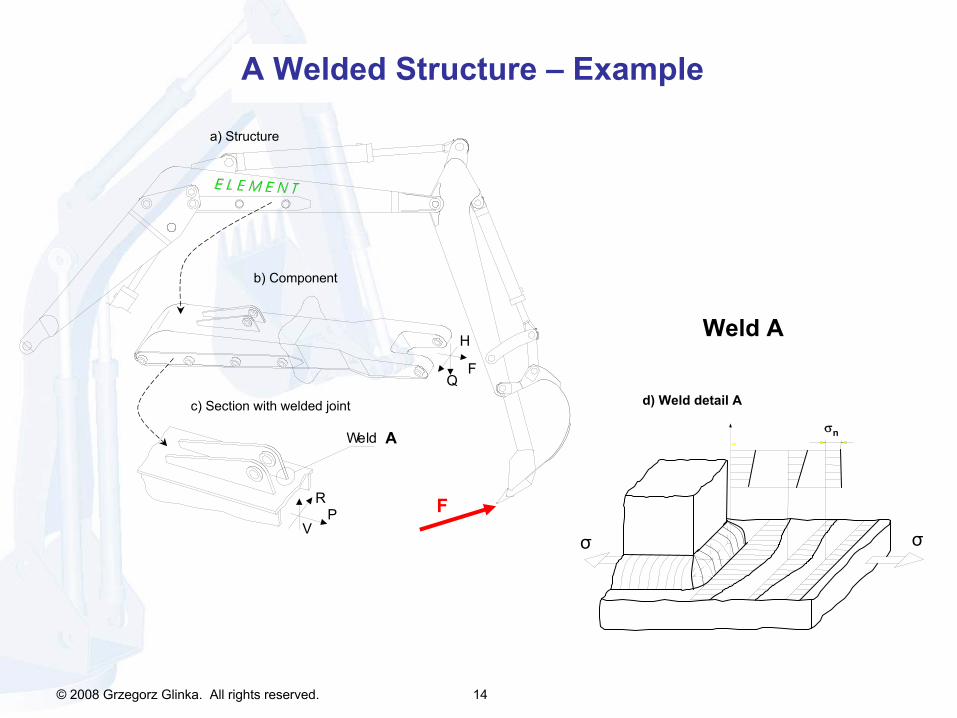
© 2008 Grzegorz Glinka. All rights reserved. 14
A Welded Structure –
Example
VP
Q
R
H
F
Weld
a) Structure
b) Component
c) Section with welded joint
Aσn
d) Weld detail A
Weld A
σσ
F
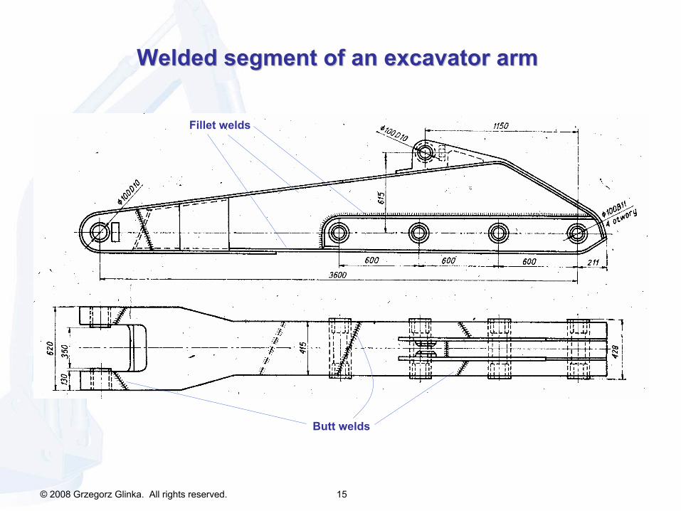
© 2008 Grzegorz Glinka. All rights reserved. 15
Fillet welds
Butt welds
Welded segment of an excavator Welded segment of an excavator armarm
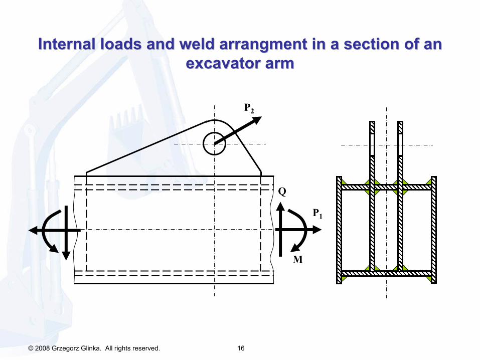
© 2008 Grzegorz Glinka. All rights reserved. 16
P1
P2
M
Q
Internal loads and weld arrangmentInternal loads and weld arrangment
in a section of an in a section of an excavator armexcavator arm
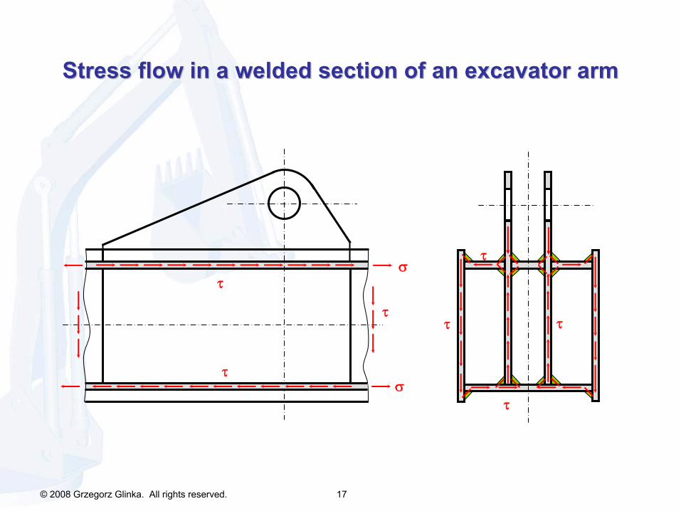
© 2008 Grzegorz Glinka. All rights reserved. 17
Stress flowStress flow
in a in a welded welded section of an excavator armsection of an excavator arm
σ
τ
τ
τ
σ
τ
τ
τ
τ
© 2008 Grzegorz Glinka. All rights reserved. 18
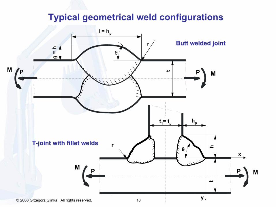
g =
hθ
r
t
l = hp
PP MM
Typical geometrical weld configurations
TT--joint with fillet weldsjoint with fillet welds
Butt welded jointButt welded joint
t
r
t1
= tp
θ
hp
h
PP
y
x
MM
© 2008 Grzegorz Glinka. All rights reserved. 19
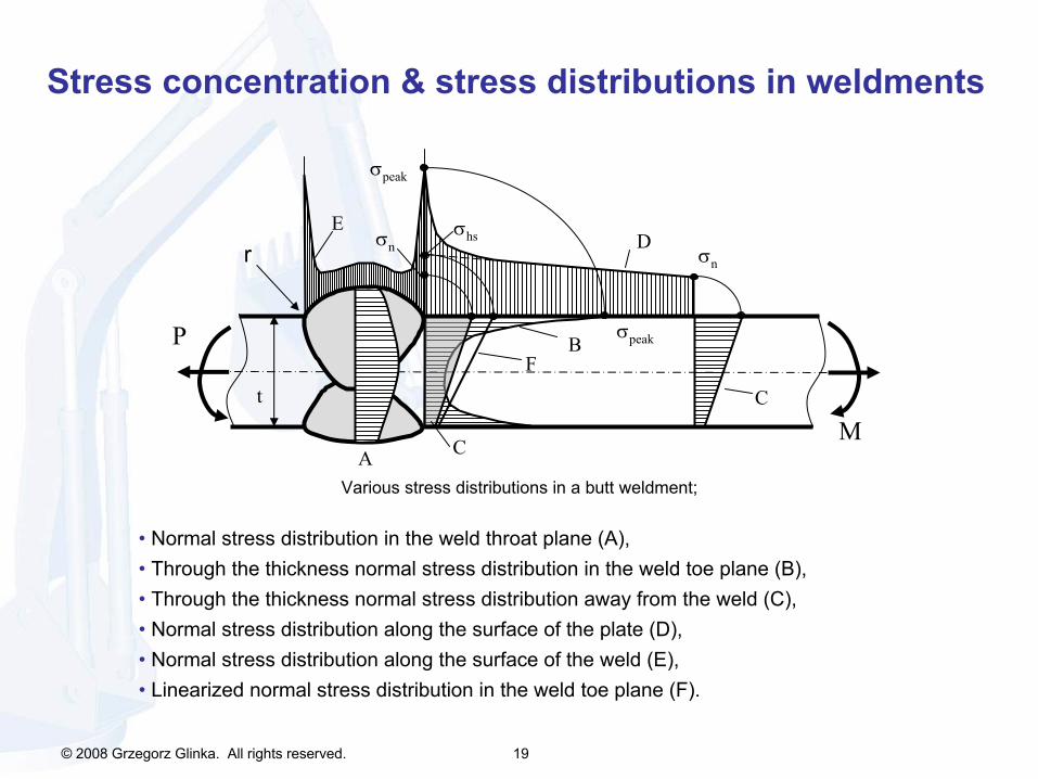
Stress concentration & stress distributions in weldments
Various stress distributions in a butt weldment;
r
A
B
C
DE
P
M
F
σpeak
σhs
σn
σpeak
t
C
σn
• Normal stress distribution in the weld throat plane (A), • Through the thickness normal stress distribution in the weld toe plane (B), • Through the thickness normal stress distribution away from the weld (C),• Normal stress distribution along the surface of the plate (D),• Normal stress distribution along the surface of the weld (E), • Linearized normal stress distribution in the weld toe plane (F).
© 2008 Grzegorz Glinka. All rights reserved. 20
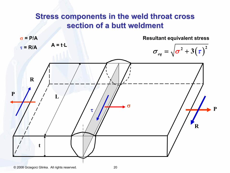
Stress components in the weld throat cross Stress components in the weld throat cross section of a butt weldmentsection of a butt weldment
P
R
στ
L
t
R
P
σ
= P/A
τ
= R/A
Resultant equivalent stress
( )eq22 3σσ τ= +
A = t·L
© 2008 Grzegorz Glinka. All rights reserved. 21
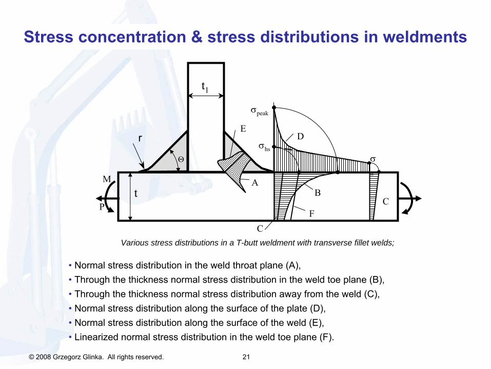
Various stress distributions in a T-butt weldment with transverse fillet welds;
r
t
t1
ED
BC
A
σpeak
σn
σhs
FP
M
C
Θ
• Normal stress distribution in the weld throat plane (A), • Through the thickness normal stress distribution in the weld toe plane (B), • Through the thickness normal stress distribution away from the weld (C),• Normal stress distribution along the surface of the plate (D),• Normal stress distribution along the surface of the weld (E), • Linearized normal stress distribution in the weld toe plane (F).
Stress concentration & stress distributions in weldments
© 2008 Grzegorz Glinka. All rights reserved. 22
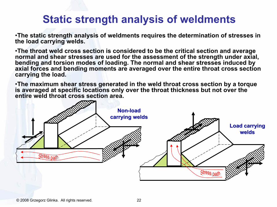
Static strength analysis of weldments•The static strength analysis of weldments requires the determination of stresses in the load carrying welds. •The throat weld cross section is considered to be the critical section and average normal and shear stresses are used for the assessment of the strength under axial, bending and torsion modes of loading. The normal and shear stresses induced by axial forces and bending moments are averaged over the entire throat cross section carrying the load. •The maximum shear stress generated in the weld throat cross section by a torque is averaged at specific locations only over the throat thickness
but not over the entire weld throat cross section area.
NonNon--load load carrying weldscarrying welds
Load carrying Load carrying weldswelds
© 2008 Grzegorz Glinka. All rights reserved. 23
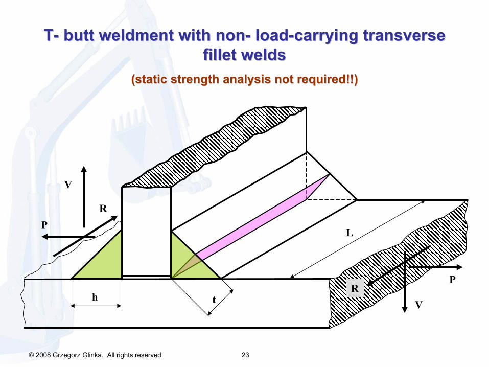
TT--
butt weldment with nonbutt weldment with non--
loadload--carrying transverse carrying transverse fillet welds fillet welds
(static strength analysis not required!!)(static strength analysis not required!!)
RV
P
L
t
R
V
P
h
© 2008 Grzegorz Glinka. All rights reserved. 24
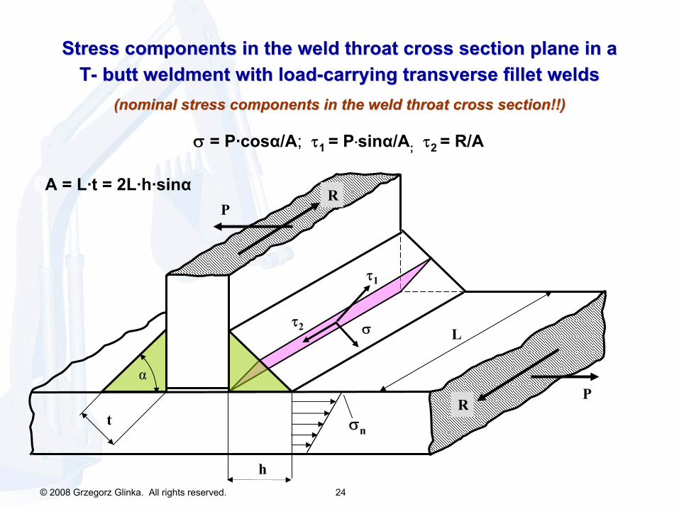
Stress components in the weld throat cross section plane in a Stress components in the weld throat cross section plane in a TT--
butt weldment with loadbutt weldment with load--carrying transverse fillet weldscarrying transverse fillet welds(nominal stress components in the weld throat cross section!!)(nominal stress components in the weld throat cross section!!)
A = L·t
= 2L·h·sinα
τ1
στ2
RP
L
t
RP
σn
α
h
σ
= P·cosα/A; τ1 = P·sinα/A; τ2 = R/A
© 2008 Grzegorz Glinka. All rights reserved. 25
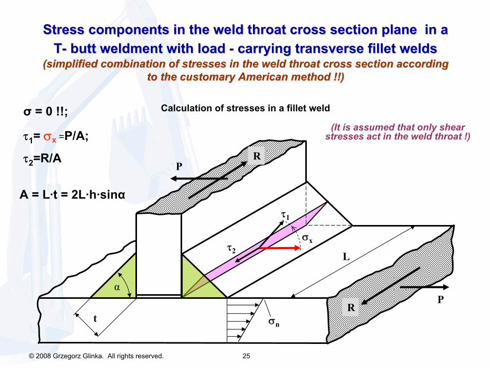
Stress components in the weld throat cross section plane in a Stress components in the weld throat cross section plane in a TT--
butt weldment with load butt weldment with load --
carrying transverse fillet weldscarrying transverse fillet welds
(simplified combination of stresses in the weld throat cross sec(simplified combination of stresses in the weld throat cross section according tion according
to the customary American method !!)to the customary American method !!)
σ
= 0 !!;
τ1
= σX
=P/A;
τ2
=R/A
Calculation of stresses in a fillet weld
τ1
σxτ2
RP
L
t
RP
σn
α
(It is assumed that only shear stresses act in the weld throat !)
A = L·t
= 2L·h·sinα
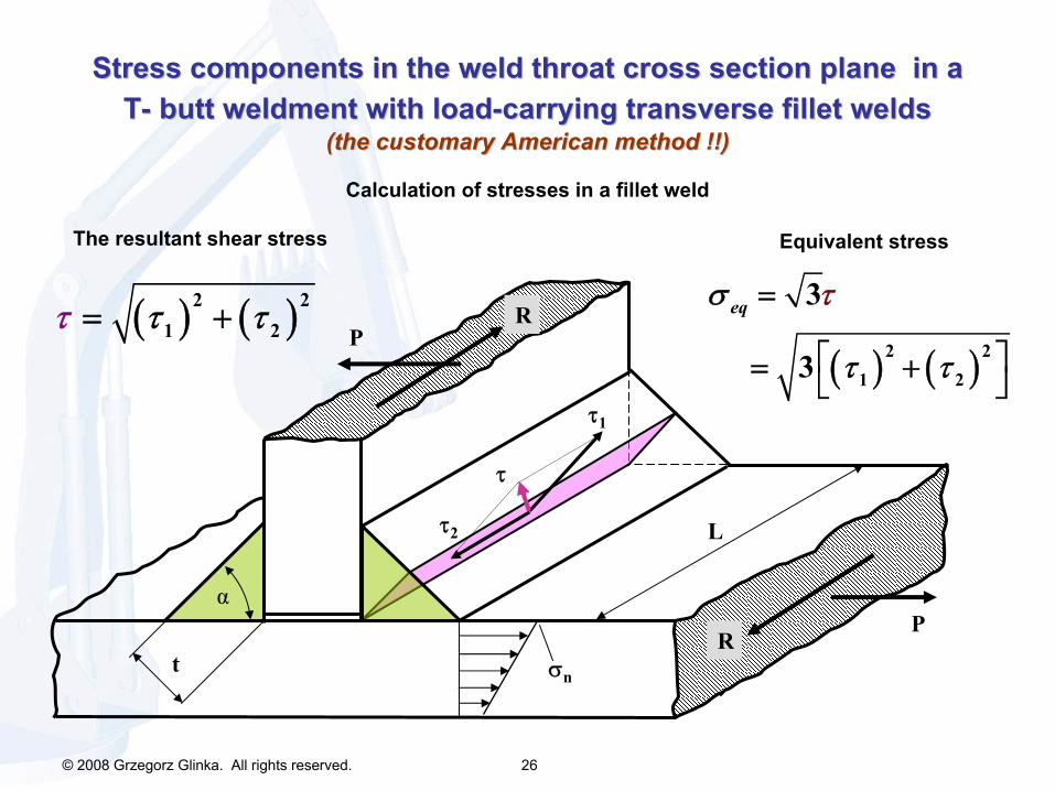
© 2008 Grzegorz Glinka. All rights reserved. 26
Stress components in the weld throat cross section plane in a Stress components in the weld throat cross section plane in a TT--
butt weldment with loadbutt weldment with load--carrying transverse fillet weldscarrying transverse fillet welds
(the customary American method !!)(the customary American method !!)
τ1
τ2
RP
L
t
RP
σn
α
τ
( ) ( )2 21 2ττ τ= +
( ) ( )2 21 2
3
3
eqσ τ
τ τ
=
⎡ ⎤= +⎣ ⎦
Equivalent stressThe resultant shear stress
Calculation of stresses in a fillet weld

© 2008 Grzegorz Glinka. All rights reserved. 27
b)
c)
Fillet welds under primary shear and bending loadFillet welds under primary shear and bending load
2
1,
2
2M
MM
dV l V lt b dt b d
M cIσ
τ σ
⋅ ⋅ ⋅= = ⋅ ⋅⋅ ⋅⋅=
=
σV
σV
σM
V
σM
d)
shear shear
σV
V
σV
1,
V
VV
Vt bσ
τ σ
=⋅
=
M
σM
σM
bending bending
ht
b
d
l
V
α
a)
© 2008 Grzegorz Glinka. All rights reserved. 28
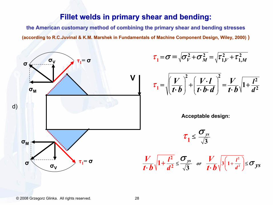
Fillet welds in primary shear and bending:Fillet welds in primary shear and bending:the American customary method of combining the primary shear andthe American customary method of combining the primary shear and
bending stressesbending stresses
(according to (according to R.C.JuvinalR.C.Juvinal
& K.M. & K.M. MarshekMarshek
in Fundamentals of Machine Component Design, Wiley, 2000)in Fundamentals of Machine Component Design, Wiley, 2000)
))
2 2 2 21, 1,
222
2
1
1 1
V M V M
ld
V V l Vt b t b d t b
τ
τ
σ σ σ τ τ
⎛ ⎞⎛ ⎞⎜ ⎟⎜ ⎟⎜ ⎟⎜ ⎟
⎝ ⎠ ⎝ ⎠
= + = +
= + = +
=
⋅⋅ ⋅ ⋅ ⋅
Acceptable design:
2
2
2
2 3 1
1 3
31
ys
ys or ld ys
ld
V Vt b t b σ
τ σ
σ ⎛ ⎞+⎜ ⎟
⎝≤
⎠≤
≤
+⋅ ⋅
d)
σV
σM
V
σ τ1
= σ
σV
σM
σ τ1
= σ

© 2008 Grzegorz Glinka. All rights reserved. 29
22
2M
dV l V lt b dt b d
M cIσ
⋅ ⋅ ⋅= = ⋅ ⋅⋅ ⋅⋅=V
Vt bσ = ⋅
a)
σV
V
σV
,V nσ ,V tτ
VVt bσ = ⋅
a)
σV
V
σV
,V nσ ,V tτ b)
M
σM
σM
σM.n
τM.t
b)
M
σM
σM
σM.n
τM.t
2 2
, , , ,
2 2 222
2 2 1
3
45
2
eq ysV n M n V t M t
eq ysV V M M
for
V l lt b d d
σ σ σ τ τ σ
α
σ σ σ σ σ σ
⎛ ⎞ ⎛ ⎞⎜ ⎟ ⎜ ⎟⎝ ⎠ ⎝ ⎠
⎛ ⎞⎜ ⎟
⎛ ⎞⎜ ⎟⎜ ⎟⎝ ⎠
⎝ ⎠
= + +
− +⋅
− ≤
=
= − + = ≤
Fillet welds in primary shear and bending:Fillet welds in primary shear and bending:the ISO/IIW method of combining the primary shear and bending shthe ISO/IIW method of combining the primary shear and bending shear stressesear stresses

© 2008 Grzegorz Glinka. All rights reserved. 30
The AWS method: It is assumed that the weld throat is in shear for all types of load and the shear stress in the weld throat is equal to the normal stress induced by bending moment and/or the normal force and to the shear stress induced by the shear force and/or the torque. There can be only two shear stress components
acting in the throat plane -
namely τ1
and τ2
. Therefore the resultant shear stress can be determined as:
2 21 2τ τ τ= +
The weld is acceptable if :
3ys
ys
στ τ< =
Where:
τys
is the shear yield strength of the: weld metal for fillet welds
and parent metal for butt welds
Static Strength Assessment of Fillet WeldsStatic Strength Assessment of Fillet Welds

© 2008 Grzegorz Glinka. All rights reserved. 31
Stress components in the weld throat cross section plane in a Stress components in the weld throat cross section plane in a TT--
butt weldment with loadbutt weldment with load--carrying transverse fillet weldscarrying transverse fillet welds(correct solid mechanics combination of stresses in the weld thr(correct solid mechanics combination of stresses in the weld throat oat ––
the the European approach)European approach)
τ1
στ2
RP
L
t
RP
σn
σ
= Pcosα/A
τ1 = Pcosα/A
τ2 = R/A
A = 2L·t·cosα
α
Resultant equivalent stress
( ) ( )2 221 23eqσ σ τ τ⎡ ⎤= + +⎣ ⎦

© 2008 Grzegorz Glinka. All rights reserved. 32
The IIW/ISO Method:
International Welding Institute employs a method in which the stresses are resolved into three components across the weld throat. These components of the stress tensor are the normal stress component σ
perpendicular to the throat plane, the shear stress τ2
acting in the throat parallel to the axis of the weld and a shear stress component τ1
acting in the throat plane and being perpendicular to the longitudinal axis of the weld. The proposed formula for calculating the equivalent
stress is:
( )2 2 21 1 23eqσ β σ τ τ= + +
The weld is acceptable if : eq ysσ σ<Where: σys
is the yield strength of the: weld metal for fillet welds and parent metal for butt welds The β
coefficient is accounting for the fact that fillet welds are slightly stronger that it is suggested by the equivalent stress σeq
.
β
= 0.7
for steel material with the yield strength σys
< 240 MPa
β
= 0.8
for steel material with the yield strength 240 < σys
< 280 MPa
β
= 0.85
for steel material with the yield strength 280 < σys
< 340 MPa
β
= 1
for steel material with the yield strength 340 < σys
< 400 MPa
Static strength assessment of fillet welds
© 2008 Grzegorz Glinka. All rights reserved. 33
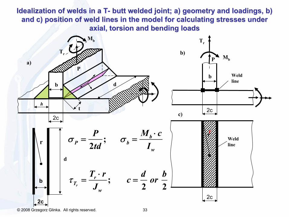
Idealization of welds in a TIdealization of welds in a T--
butt welded joint; a) geometry and loadings, b) butt welded joint; a) geometry and loadings, b) and c) position of weld lines in the model for calculating stresand c) position of weld lines in the model for calculating stresses under ses under
axial, torsion and bending loadsaxial, torsion and bending loads
Mb
Tr
b Weldline
Weldline
b)
c)
r
2c
r
d
a)
t
d
Tr
b
Mb
h
P
;2
;2 2r
bP b
w
rT
w
M cPtd I
T r d bc orJ
σ σ
τ
⋅= =
⋅= =
r
2c2c
2c
P
b

© 2008 Grzegorz Glinka. All rights reserved. 34
( ) ( )22 3reqv M P T V yield IIWσ β σ σ τ τ σ= + + + ≤ −
P
M
Tr
z
x
y
a)
r
Aw
ApV
Pw
PA
σ =,
yM
w x
M cI
σ =
max
,r
rT
w CG
T rJ
τ = Vx
VQI t
τ =
τ(x,y)
x
y
CG
b)
y
z
σ(x,y)
c)
r
( )3r
ysT V P M yield AWS
στ τ τ σ σ τ= + + + < ≤ −
Combination of stress components induced by multiple loading modCombination of stress components induced by multiple loading modeses

© 2008 Grzegorz Glinka. All rights reserved. 35
1 2
2 cos
2 cos45
1.414
xPlt
PlhP
lhPlh
τ σ
θ
= =
=
=
=
13
31.41
.2254
1
eq
Plh
Plh
σ τ= =
≈
EXAMPLE:EXAMPLE:
Transverse fillet weld under axial loadingTransverse fillet weld under axial loading
τ1
σx
σx
P/2θ
P/2
t
h
l
P
P/2
P/2
h
AWSAWS
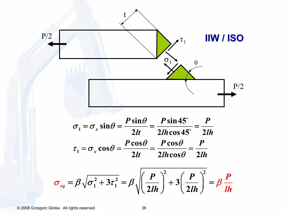
© 2008 Grzegorz Glinka. All rights reserved. 36
1
1
sin sin45sin2 2 cos45 2cos coscos2 2 cos 2
x
x
P P Plt lh lh
P P Plt lh lh
θσ σ θ
θ θτ σ θθ
= = = =
= = = =
2 22 21 13 3
2 2eqP Plh l
Ph lh
β σ τ βσ β⎛ ⎞ ⎛ ⎞= + = + =⎜ ⎟ ⎜ ⎟⎝ ⎠ ⎝ ⎠
σ1
P/2
t
τ1
P/2
θ
IIW / ISOIIW / ISO

© 2008 Grzegorz Glinka. All rights reserved. 37
2) Outline of contemporary fatigue analysis 2) Outline of contemporary fatigue analysis methods methods ––
similarities, differences and similarities, differences and
limitations, limitations,
•the classical nominal stress method (S S --
NN),
• the local strain-life approach,(εε
––
NN)
• the fracture mechanics approach (da/dNda/dN
––
ΔΔKK),
© 2008 Grzegorz Glinka. All rights reserved. 38
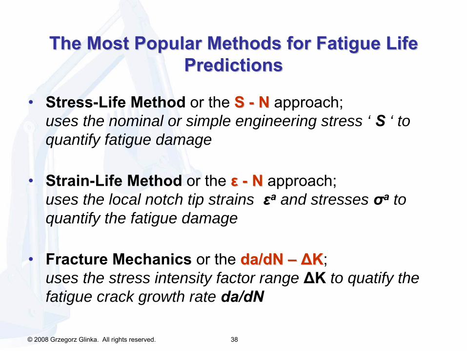
•
Stress-Life Method
or the S S --
NN
approach; uses the nominal or simple engineering stress ‘ S
‘ to
quantify fatigue damage
•
Strain-Life Method
or the εε
--
NN
approach; uses the local notch tip strains εa
and stresses σa
to quantify the fatigue damage
•
Fracture Mechanics
or the da/dNda/dN
––
ΔΔKK; uses the stress intensity factor range ΔK
to quatify the fatigue crack growth rate da/dN
The Most Popular Methods for Fatigue Life The Most Popular Methods for Fatigue Life PredictionsPredictions

© 2008 Grzegorz Glinka. All rights reserved. 39
Information Path for Strength and Fatigue Life AnalysisInformation Path for Strength and Fatigue Life Analysis
ComponentGeometry
LoadingHistory
Stress-StrainAnalysis
Damage Analysis
Fatigue Life
MaterialProperties
© 2008 Grzegorz Glinka. All rights reserved. 40
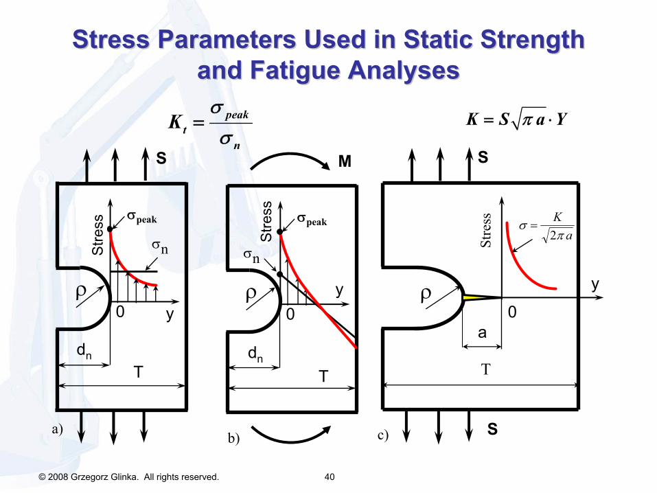
Stress Parameters Used in Static Strength Stress Parameters Used in Static Strength and Fatigue Analysesand Fatigue Analyses
peakt
n
Kσσ
=
a)
σn
y
dn
0
T
ρ
σpeak
Stre
ss
S
K S a Yπ= ⋅
c)
y
a0
T
ρ
Stre
ss σπ
=Ka2
S
S
σn
y
dn
0
T
ρ
σpeak
Stre
ss
M
b)
© 2008 Grzegorz Glinka. All rights reserved. 41
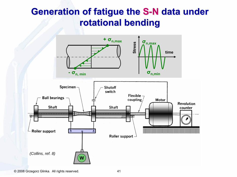
Generation of fatigue the Generation of fatigue the SS--NN
data under data under rotational bending rotational bending
-
σn, min
+ σn,max σn,max
σn,min
timeStre
ss
(Collins, ref. 8)W
© 2008 Grzegorz Glinka. All rights reserved. 42
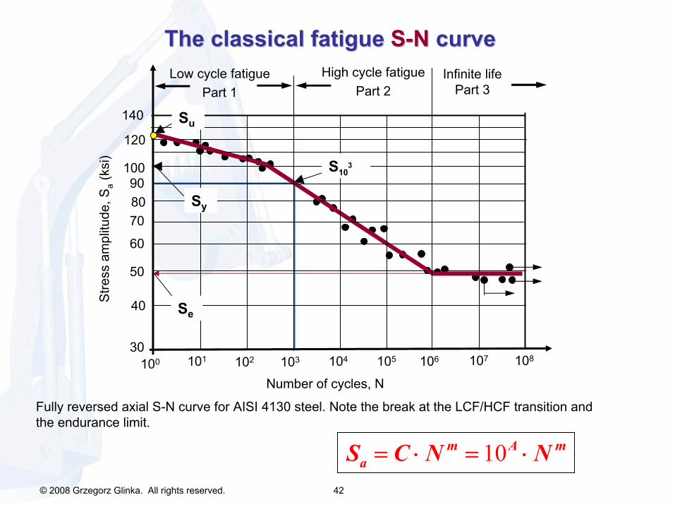
Fully reversed axial S-N curve for AISI 4130 steel. Note the break at the LCF/HCF transition and the endurance limit.
10m A maS C N N= ⋅ = ⋅
The classical fatigue The classical fatigue SS--NN
curvecurve
Number of cycles, N
Stre
ss a
mpl
itude
, Sa
(ksi
)
Low cycle fatiguePart 1
Infinite
life
Part 3
100 101 102 103 104 105 106 107 10830
40
50
60
708090
100
120
140
High cycle fatiguePart 2
Sy
Se
Su
S103

© 2008 Grzegorz Glinka. All rights reserved. 43
''2 22
b cf N Nf f fE
σε ε⎛ ⎞ ⎛ ⎞⎜ ⎟ ⎜ ⎟⎝ ⎠ ⎝ ⎠
Δ = +'
1
'n
E Kσσε
⎛ ⎞⎜ ⎟⎜ ⎟⎝ ⎠
= +
The StrainThe Strain--life and the Cyclic Stresslife and the Cyclic Stress--Strain Curve Obtained from Strain Curve Obtained from Smooth Cylindrical Specimens Tested Under Strain Control Smooth Cylindrical Specimens Tested Under Strain Control
((UniUni--axial Stress State)axial Stress State)
Strain -
Life Curve
εεε
log
(Δε/
2)
log (2Nf
)
σf
/E
εf
0 2Ne
σe
/E
c
b
0
Stress -Strain Curve
ε
σ
E

© 2008 Grzegorz Glinka. All rights reserved. 44
Determination of the Complete Fatigue Crack Growth Curve Determination of the Complete Fatigue Crack Growth Curve ((da/dNda/dN--∆∆K and K and ∆∆KKthth
))
a & b) specimens used to generate fatigue crack growth curves, c) stress history, d) fatigue crack growth rate curve.
σn
nK a Yσ π= ×W
K P a Yπ= ×
a
P
P
2a
W
a)
b)
Time
c)
P o
r σ n
0
Log(
da/d
N)
Log(ΔK)ΔKth Kmax
= Kc
m
d)
Applic
abilit
y of P
aris’
equa
tion

© 2008 Grzegorz Glinka. All rights reserved. 45
LOADING
F
t
GEOMETRY, Kf
PSO
MATERIAL
No N
Δσn
σe
MATERIAL
σ
ε0
E
Stress-StrainAnalysis
Damage Analysis
Fatigue Life
Information path for fatigue life estimation based on the Information path for fatigue life estimation based on the SS--NN
methodmethod
© 2008 Grzegorz Glinka. All rights reserved. 46
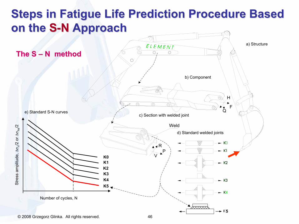
Steps in Fatigue Life Prediction Procedure Based Steps in Fatigue Life Prediction Procedure Based on the on the SS--NN
ApproachApproach
The S The S ––
N methodN method
5
e) Standard S-N curves
K0K1K2K3K4K5St
ress
am
plitu
de, Δ
σ n/2
or Δ
σ hs/2
Number of cycles, N
d) Standard welded joints
c) Section with welded joint
a) Structure
b) Component
VP
R
Q
H
F
Weld
© 2008 Grzegorz Glinka. All rights reserved. 47
( )
( )
( )
( )
( )
5
5
5
5
5
11
1 5
22
2 5
33
3 5
44
4 5
55
5 5
1
1
1
1
1
m
m
m
m
m
DN C
DN C
DN C
DN C
DN C
σ
σ
σ
σ
σ
Δ= =
Δ= =
Δ= =
Δ= =
Δ= =
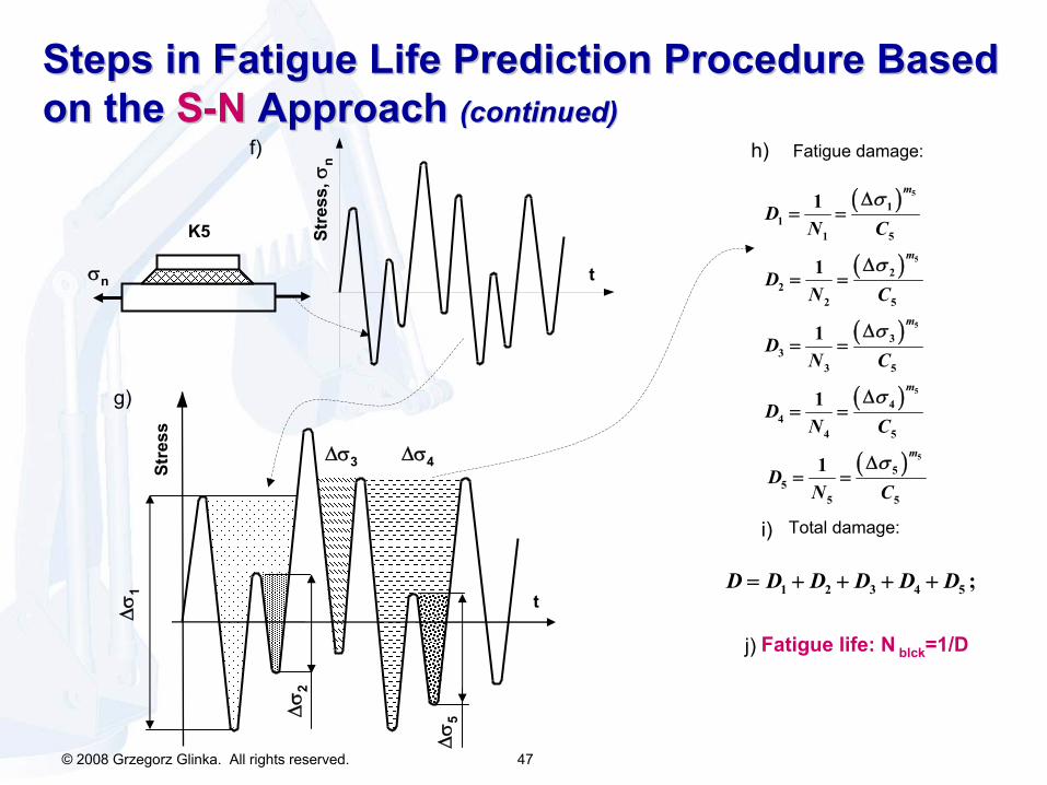
1 2 3 4 5 ;D D D D D D= + + + +
Δσ 1
Δσ 2
Δσ3 Δσ4Δ
σ 5
Stre
ss
t
g)
Fatigue damage:h)
Total damage:i)
Fatigue life: N
blck
=1/Dj)
Stre
ss, σ
n
f)
t
K5
σn
Steps in Fatigue Life Prediction Procedure Based Steps in Fatigue Life Prediction Procedure Based on the on the SS--NN
Approach Approach (continued)(continued)

© 2008 Grzegorz Glinka. All rights reserved. 48
a) Structure
Q
H
F
K 5
σn
The Similitude Concept
states that if the nominal stress histories in the structure and in the test specimen are the same, then the fatigue response in each case will also be the same and can be described by the generic S-N curve. It is assumed that such an approach accounts also for the stress concentration, loading sequence effects, manufacturing etc.
K0K1K2K3K4K5St
ress
am
plitu
de, Δ
σ n/2
or Δ
σ hs/2
Number of cycles, N0
The Similitude Concept in the The Similitude Concept in the SS--NN
MethodMethod
© 2008 Grzegorz Glinka. All rights reserved. 49
LOADING
F
t
GEOMETRY, Kf
PSO
MATERIAL
σ
ε0
E
Stress-StrainAnalysis
Damage Analysis
Fatigue Life
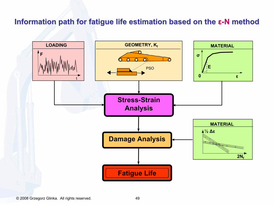
Information path for fatigue life estimation based on the Information path for fatigue life estimation based on the εε--NN
methodmethod
MATERIAL½
Δε
2Nf

© 2008 Grzegorz Glinka. All rights reserved. 50
Steps in fatigue life prediction procedure based on theSteps in fatigue life prediction procedure based on the
εε
--
NN
approachapproach
a) Structure
b) Component
c) Section with welded joint
d)
σpeak
σn
σpeak
σhs
σnσhs

© 2008 Grzegorz Glinka. All rights reserved. 51
Steps in fatigue life prediction procedure based on theSteps in fatigue life prediction procedure based on the
εε--NN
approach approach
ε
σ
3
2,2'
4
5,5'7,7'
6
8
1,1'
Fatigue damage:
1 2 3 41 2 3 4
1 1 1 1; ; ; ;D D D DN N N N
= = = =
Total damage:
1 2 3 4 ;D D D D D= + + +
Fatigue life: Fatigue life: NN blckblck
=1/D=1/D
0
ε
σ
'1
'
n
E Kσ σε ⎛ ⎞= + ⎜ ⎟
⎝ ⎠
e)
( ) ( )'
'2 22
Δ= +
b cff f fN N
Eσε ε
σe
/E
log
(Δε/
2)
log (2Nf
)
σf
/E
εf
02Ne
2N
( )2
: = ×peakNeuberE
σσ ε
Δσpe
ak
t
1
2
3
4
5
6
7
8
1'
f)
( )
( )( )( )
' '
' '
'
'
,
,
,
?,?
Δ ΔΔ
f f
f f
f
f
fN
ε ε
σ σ
ε ε
ε μ σ
σ μ σ
ε μ σ
Δσ
σ
ε
Δε p Δε e= Δσ/Ε
Δε
0
© 2008 Grzegorz Glinka. All rights reserved. 52
a) Specimen
b) Notched component
εpeakx
y
z
εpeak
εpeak
( ) ( )'
'2 22
bff f fN N c
Eσε εΔ
= +
log
(Δε/
2)
log (2Nf
)
εf
0
l)
j)
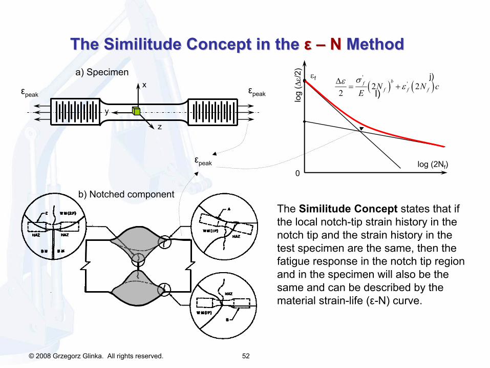
The Similitude Concept
states that if the local notch-tip strain history in the notch tip and the strain history in the test specimen are the same, then the fatigue response in the notch tip region and in the specimen will also be the same and can be described by the material strain-life (ε-N) curve.
The Similitude Concept in the The Similitude Concept in the εε
––
NN
MethodMethod

© 2008 Grzegorz Glinka. All rights reserved. 53
Information path for fatigue life estimation Information path for fatigue life estimation based on the based on the da/dNda/dN--ΔΔKK
methodmethod
LOADING
F
t
GEOMETRY, Kf
PSO
MATERIAL
σ
ε0
E
Stress-StrainAnalysis
Damage Analysis
Fatigue Life
MATERIAL
n
ΔKΔKth
dadN

© 2008 Grzegorz Glinka. All rights reserved. 54
VP
Q
R
H
F
Weld
a) Structure
b) Component
c) Section with welded joint
ΔS1
ΔS2
ΔS3 ΔS4
ΔS5
Stre
ss, S
t
e)
d)
Steps in the Fatigue Life Prediction Procedure Based Steps in the Fatigue Life Prediction Procedure Based on the on the da/dda/dNN--ΔΔKK
ApproachApproach
© 2008 Grzegorz Glinka. All rights reserved. 55
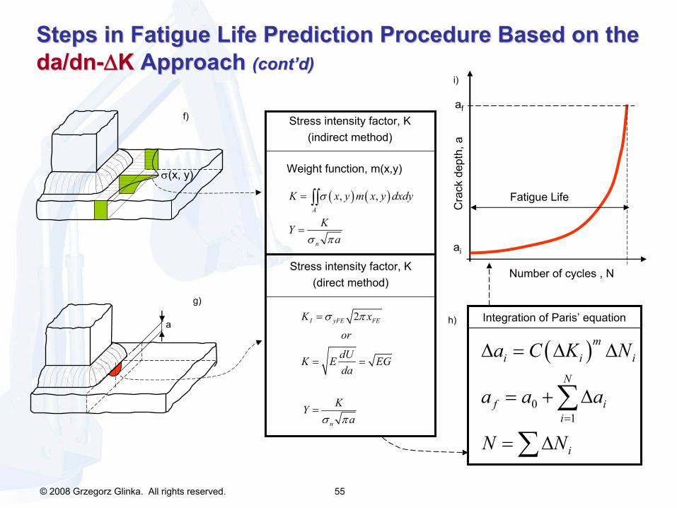
Stress intensity factor, K(indirect method)
Weight function, m(x,y)
( ) ( ), ,A
n
K x y m x y dxdy
KYa
σ
σ π
=
=
∫∫
Stress intensity factor, K(direct method)
2I yFE FE
n
K x
or
dUK E EGda
KYa
σ π
σ π
=
= =
=
σ(x, y)
f)
a
g)
( )
01
mi i i
N
f ii
i
a C K N
a a a
N N=
Δ = Δ Δ
= + Δ
= Δ
∑
∑
Integration of Paris’
equationh)
af
ai
Number of cycles , N
Cra
ck d
epth
, a
Fatigue Life
i)
Steps in Fatigue Life Prediction Procedure Based on the Steps in Fatigue Life Prediction Procedure Based on the da/dnda/dn--ΔΔKK
Approach Approach (cont(cont’’d)d)
© 2008 Grzegorz Glinka. All rights reserved. 56
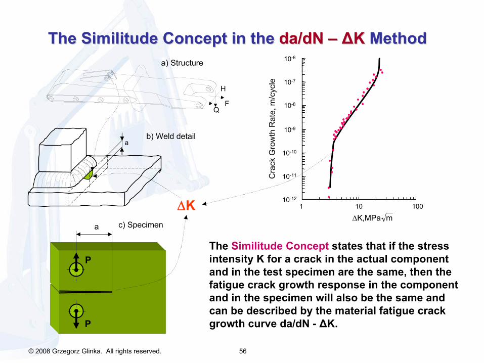
The Similitude Concept
states that if the stress intensity K for a crack in the actual component and in the test specimen are the same, then the fatigue crack growth response in the component and in the specimen will also be the same and can be described by the material fatigue crack growth curve da/dN
-
ΔK.
a) Structure
Q
H
F
ab) Weld detail
c) Specimena
P
P
ΔK 10-12
10-11
10-10
10-9
10-8
10-7
10-6
1 10 100
Cra
ck G
row
th R
ate,
m/c
ycle
mMPa,KΔ
The Similitude Concept in the The Similitude Concept in the da/dNda/dN
––
ΔΔKK
MethodMethod

© 2008 Grzegorz Glinka. All rights reserved. 57
What stress parameter is needed for the Fracture What stress parameter is needed for the Fracture Mechanics based (Mechanics based (da/dNda/dN--ΔΔKK) fatigue analysis?) fatigue analysis?
x
a0
T
ρ
Stre
ss σ
(x) ( )
2x
xKσπ
=
S
SThe Stress Intensity Factor K
characterizing the stress field in the crack tip region is needed!
The
K
factor can be obtained from:-
ready made Handbook solutions (easy to use but often inadequate for the analyzed problem)
-
from the
σ(x)
near crack tip stress or
displacement data obtained from FE analysis of a cracked body (difficult)
-
from the weight function by using the FE stress analysis data of un-cracked body (versatile and suitable for FCG analysis)
© 2008 Grzegorz Glinka. All rights reserved. 58
3) Load/stress histories3) Load/stress histories•
methods of assembling characteristic load/stress
histories,
• the rainflow
counting method –
live example,
•
extraction of load/stress cycles from the frequency domain data.
© 2008 Grzegorz Glinka. All rights reserved. 59
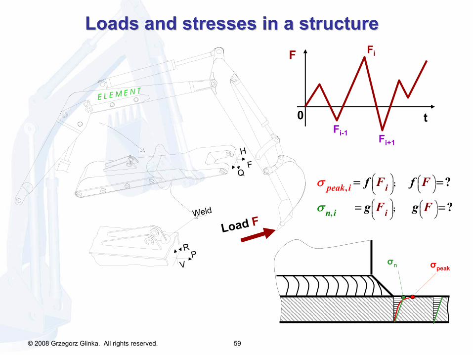
Loads and stresses in a structureLoads and stresses in a structure
Load F
VP
Q
R
HF
Weld
;
;,
, ?
?i
i
ak
n
p
i
e i F F
F F
f f
g gσ
σ ⎛ ⎞ ⎛ ⎞⎜ ⎟⎜ ⎟ ⎝ ⎠⎝ ⎠
⎛ ⎞ ⎛ ⎞⎜ ⎟⎜ ⎟ ⎝ ⎠⎝ ⎠
= =
= =
F
t
Fi
Fi+1Fi-1
0
σn σpeak

© 2008 Grzegorz Glinka. All rights reserved. 60
( )
3
3
32;
; ; ;4 2 64
b b
b
eakn pM c M
SI d
W d dM L l c I
ππ
σ σ= = = = ±
= + = =Note!
In the case of smooth components,
such as the railway axle,
the nominal stress and the local peak stress are the same!
b)
d N.A.
,min 3
32n
bMd
σπ
= +
,min 3
32n
bMd
σπ
= −
1
2
3
σn,max
σn,min
timeStre
ss σn,a
1 cyclec)
1
2
3
AB
y
x
Ll
Moment Mb
a)
RARB
W/2W/2 W/2
W
The load W and the nominal stress The load W and the nominal stress σσnn
in an railway axlein an railway axle

© 2008 Grzegorz Glinka. All rights reserved. 61
Loads and StressesLoads and StressesThe load, the nominal stress, the local peak stress and the streThe load, the nominal stress, the local peak stress and the stress concentration factorss concentration factor
, ,
;
;
; ;
;
;
;
1
;
peaktF F
Fpeak i i
F
Fn i i
nnet
n F
Fn
Fpe
et
ak
h h KF
hk F F
k
FA
k F
k A
h F
σ
σ σ
σ σ
σ
= =
==
=
=
=
=
Axial load –
linear elastic analysis
σn
y
dn
0
T
ρ
σpeak
Stre
ss
F
F
Analytical, FEMAnalytical, FEM HndbkHndbk

© 2008 Grzegorz Glinka. All rights reserved. 62
Loads and StressesLoads and StressesThe load, the nominal stress, the local peak stress and the streThe load, the nominal stress, the local peak stress and the stress concentration factorss concentration factor
, ,
,
;
;
; ;
btMpeak i pe Mi ak i i
netn
net
n M
netM Mn i i
net
M or kh M K
M cI
k M
ck k MI
σ σ
σ
σ
σ
= = ⋅
⋅=
=
= ⇒ =
Bending load –
linear elastic analysis
σn
y
dn
0
T
ρ
σpeak
Stre
ssM
b) M

© 2008 Grzegorz Glinka. All rights reserved. 63
peak eakt t
n
poK rS
Kσ
σσ
= =
Kt
–
stress concentration factor (net or gross, net Kt ≠
gross Kt
!!
)
σpeak
–
stress at the notch tip
σn
-
net nominal stress
S -
gross nominal stress
Stress Concentration Factors in Fatigue AnalysisStress Concentration Factors in Fatigue AnalysisThe nominal stress and the stress concentration factor in simpleThe nominal stress and the stress concentration factor in simple
load/geometry configurationsload/geometry configurations
nnet gross
P Por SA A
σ = =
grossnetn
net gross
M cM cor S
I Iσ
⋅⋅= =
Simple axial load
Pure bending load
σn
y
dn
0
T
r
σpeak
Stre
ss
S
S
TensionTension
σn
y
dn
0
T
r
σpeak
Stre
ss
MS
SM
BendingBending
net Ktgross Kt
© 2008 Grzegorz Glinka. All rights reserved. 64
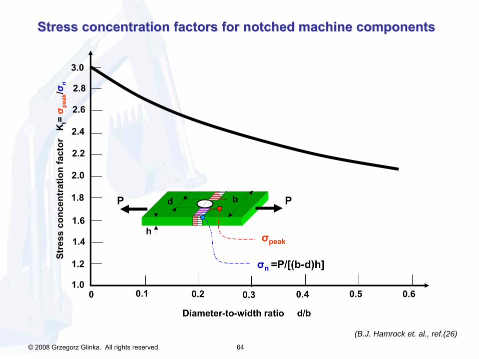
Stress concentration factors for notched machine componentsStress concentration factors for notched machine components
(B.J. Hamrock et. al., ref.(26)
d b
h
1.0
1.4
1.8
1.2
1.6
2.0
2.2
2.4
2.6
2.8
3.0St
ress
con
cent
ratio
n fa
ctor
K
t=σ p
eak/σ
n
Diameter-to-width ratio d/b
0 0.1 0.2 0.3 0.4 0.5 0.6
σpeak
P P
σn
=P/[(b-d)h]
© 2008 Grzegorz Glinka. All rights reserved. 65
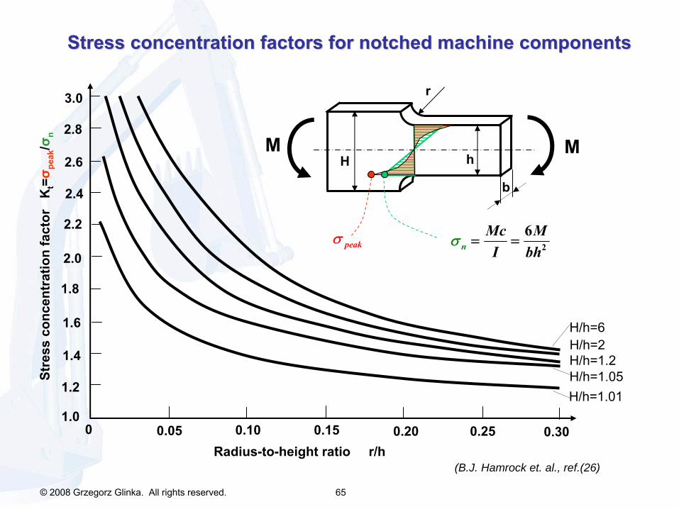
Stress concentration factors for notched machine componentsStress concentration factors for notched machine components
(B.J. Hamrock et. al., ref.(26)
1.0
1.4
1.8
1.2
1.6
2.0
2.2
2.4
2.6
2.8
3.0
0 0.05 0.10 0.15 0.20 0.25 0.30
H/h=6H/h=2H/h=1.2H/h=1.05H/h=1.01
Stre
ss c
once
ntra
tion
fact
or
Kt=σ p
eak/σ
n
Radius-to-height ratio r/h
peakσ
r
Mh
b
MH
2
6n
Mc MI bh
σ = =

© 2008 Grzegorz Glinka. All rights reserved. 66
Loads and StressesLoads and StressesThe load, the nominal stress, the local peak stress and the streThe load, the nominal stress, the local peak stress and the stress concentration factorss concentration factor
,
,
, ;
;
;i
bti
t
F Mn i i
tpeak i
F Mpea
i
F M
k
i
ii
M
M
K
k F k
K
h
M
k F kor
hF
σ
σ
σ
= +
= ⋅ +
= +
Simultaneous axial and bending load
σn
y
dn
0
T
ρ
σpeak
Stre
ss
M
b) M
F
F
;
,
,
,
;
;
bt
tt
F M
F M
K
h
k
K
h
k From simple analytical stress analysis
From stress concentration handbooks
From detail FEM analysis
© 2008 Grzegorz Glinka. All rights reserved. 67
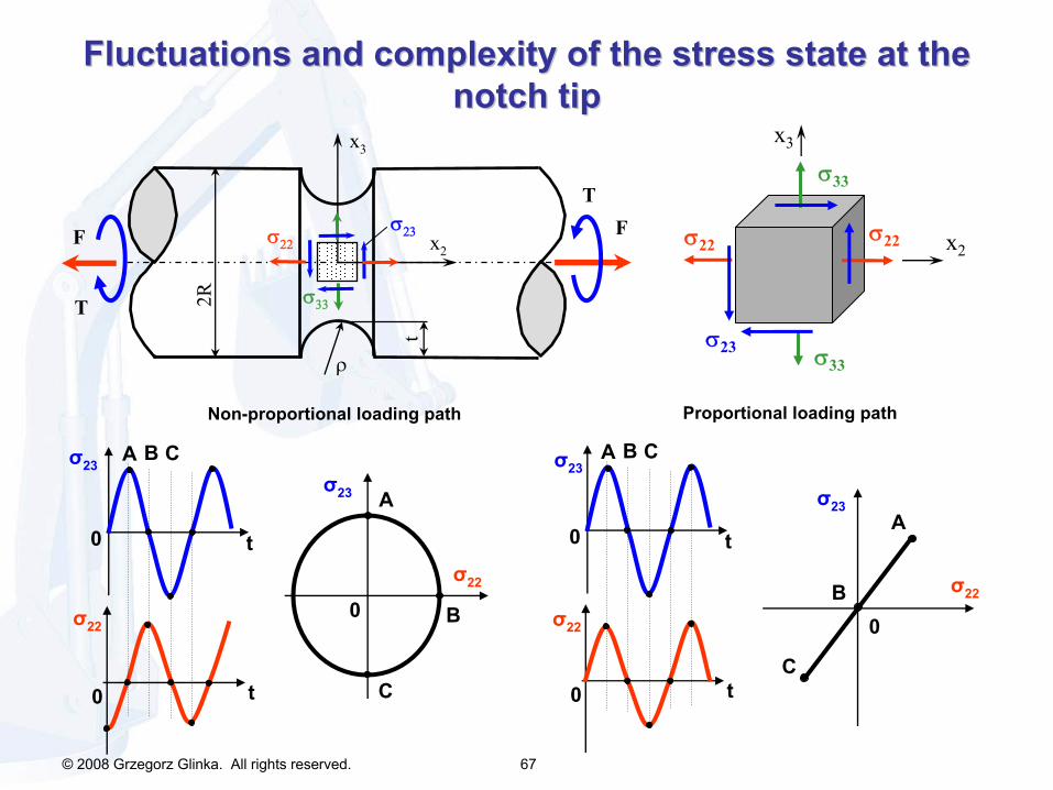
σ22
A B C
t
t
σ23
0
0
A
B
C
σ23
σ22
0
A B C
t
t
σ23
0
0
σ22
A
B
C
σ23
σ22
0
Non-proportional loading path Proportional loading path
Fσ22
σ33
ρ
2R
t
x2
x3
F
T
Tσ23 σ22
σ33
σ22
σ33
x2
x3
σ23
Fluctuations and complexity of the stress state at the Fluctuations and complexity of the stress state at the notch tipnotch tip

© 2008 Grzegorz Glinka. All rights reserved. 68
How to establish the nominal stress history?How to establish the nominal stress history?a) The analytical or FE analysis should be carried out for one characteristic load magnitude, i.e. P=1, Mb
=1, T=1 in order to establish the proportionality factors, kP
, kM
, and kT
such that:
;;= ⋅ = ⋅ = ⋅P M Tn n nP M Tbk P k M k Tσ σ τ
b) The peak and valleys of the nominal stress history σn,,i
are determined by scaling the peak and valleys load history Pi
, Mb,I
and Ti
by appropriate proportionality factors kP
, kM
, and kT
such that:
, , ,;,= ⋅ = ⋅ = ⋅P M Tn i n i n i iiP M Tb ik P k M k Tσ σ τ
c) In the case of proportional loading the normal peak and valley stresses can be added and the resultant nominal normal stress history can be established. Because all load modes in proportional loading have the same number of simultaneous reversals the resultant history has also the same number of resultant reversals as any of the single mode stress history.
;,, i Mi Pn b ik P k Mσ += ⋅ ⋅
d) In the case of non-proportional loading the normal stress histories (and separately
the shear stresses) have to be added as time dependent processes. Because each individual stress history has different number of reversals the number of reversals in the
resultant stress history can be established after the final superposition of all histories.
( ) ( ) ( )ii in P M bt tt k P k Mσ += ⋅ ⋅

© 2008 Grzegorz Glinka. All rights reserved. 69
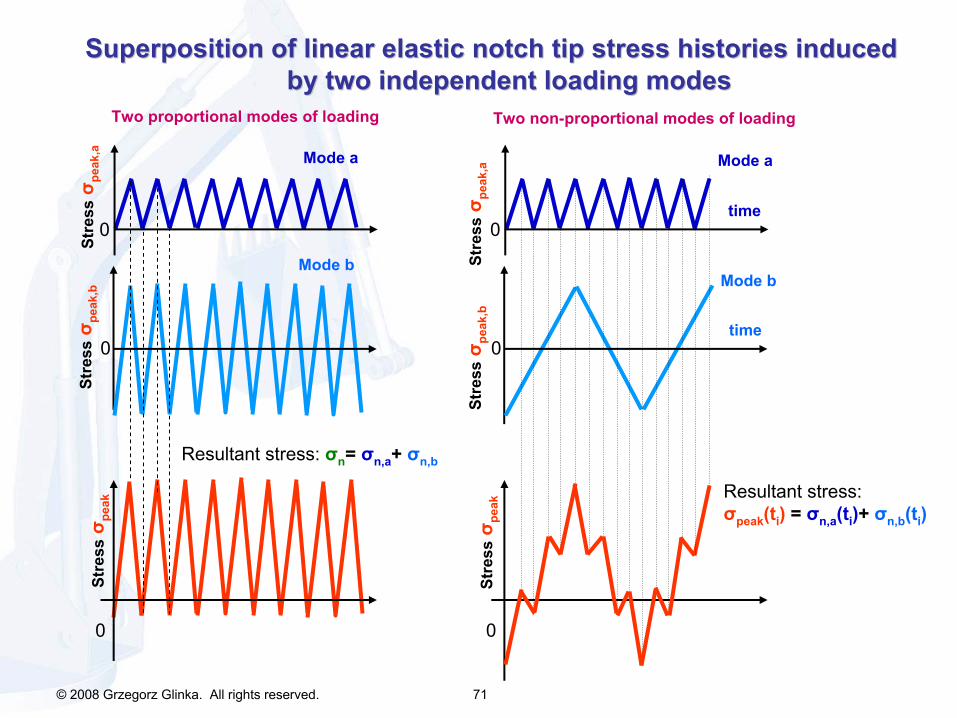
Two proportional modes of loading
0
Mode a
Stre
ss σ
n,b
0
Stre
ss σ
n,a
0
Mode b
Stre
ss σ
n
Resultant stress: σn
= σn,a
+
σn,b
0
Mode a
Stre
ss σ
n,b
0
Stre
ss σ
n,a
0
Mode b
Stre
ss σ
n
Resultant stress: σn
(ti
)= σn,a
(ti
)+
σn,b
(ti
)
time
time
Two non-proportional modes of loading
Superposition of nominal stress histories induced by two Superposition of nominal stress histories induced by two independent loading modesindependent loading modes

© 2008 Grzegorz Glinka. All rights reserved. 70
How to establish the linear elastic peak stress, How to establish the linear elastic peak stress, σσpeakpeak
,,
history?history?
a) The analytical or FE analysis should be carried out for one characteristic load magnitude, i.e. P=1, Mb
=1, T=1 in order to establish the proportionality factors, kP
, kM
, and kT
such that:
;;peak peak peaP M Tkbk P k M k Tσ σ τ= ⋅ = ⋅ = ⋅
b) The peak and valleys of the notch tip peak stress history σpeak,,i
are determined by scaling the peak and valleys load history Pi
, Mb,I
and Ti
by appropriate proportionality factors kP
, kM
, and kT
such that:;, , ,, iipeak i peak i peak iP M Tb ik P k M k Tσ σ τ= ⋅ = ⋅ = ⋅
c) In the case of proportional loading the normal peak and valley stresses can be added and the resultant notch tip normal peak stress history can be established. Because all load modes in proportional loading have the same number of simultaneous reversals the resultant history has also the same number of resultant reversals as any of the component single mode stress history.
;, ,iP Mp i bk iea k P k Mσ += ⋅ ⋅
d) In the case of non-proportional loading the normal stress histories (and separately
the shear stresses) have to be added as time dependent processes. Because each individual stress history has different number of reversals the number of reversals in the
resultant stress history can be established after the final superposition of all histories.
( ) ( ) ( )i ii P M bpeak t t tk P k Mσ += ⋅ ⋅
© 2008 Grzegorz Glinka. All rights reserved. 71
Two proportional modes of loading
0
Mode a
Stre
ssσ p
eak,
b
0
Stre
ssσ p
eak,
a
0
Mode b
Stre
ssσ p
eak
Resultant stress: σn
= σn,a
+
σn,b
0
Mode a
0
0
Mode b
Resultant stress: σpeak
(ti
)
= σn,a
(ti
)+
σn,b
(ti
)
time
time
Two non-proportional modes of loading
Superposition of linear elastic notch tip stress histories inducSuperposition of linear elastic notch tip stress histories induced ed by two independent loading modesby two independent loading modes
Stre
ssσ p
eak,
bSt
ress
σ pea
k,a
Stre
ssσ p
eak
© 2008 Grzegorz Glinka. All rights reserved. 72
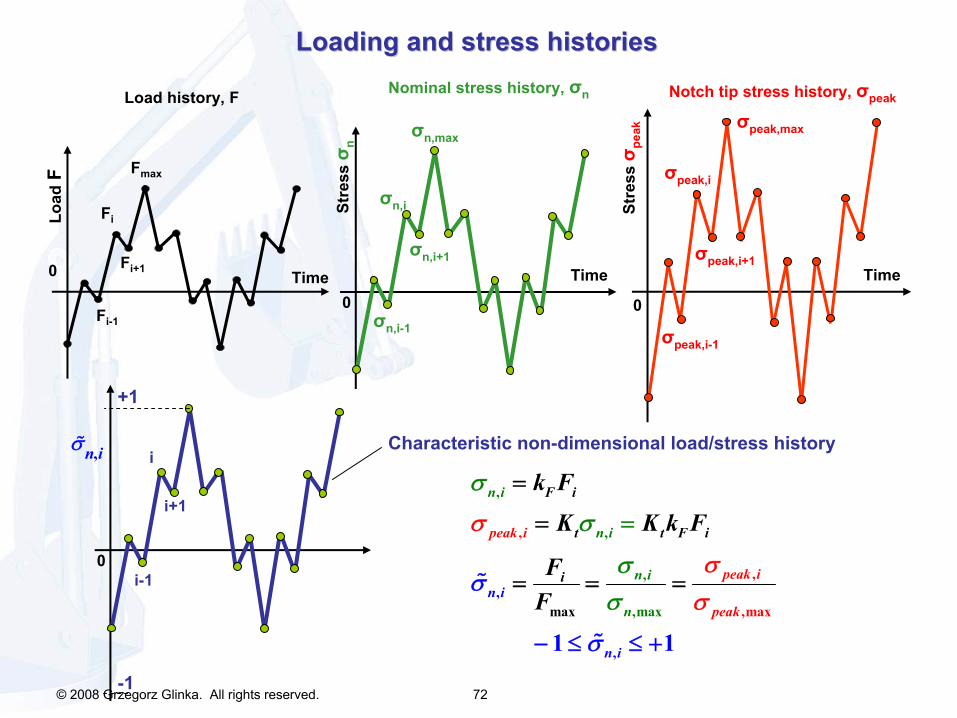
Loading and stress historiesLoading and stress histories
Time
0
Stre
ss σ
peak
Time0
Load
F
Time
Fi-1
Fi
Fi+1
Fmax
0
Stre
ss σ
n
σn,i-1
σn,i
σn,i+1
σn,max
Load history, F Nominal stress history, σn Notch tip stress history, σpeak
0i-1
i
i+1
+1
-1
,n iσ
max
,
,
,
,
,ma
,
,max,
,
x
1 1
F i
t t F i
i
peak i
peak i
p
n i
n i
n in
eakni
n i
k F
K K k F
FF
σ
σ
σ σ
σ
σ
σ
σσ
=
=
= =
=
− ≤
=
≤ +
Characteristic non-dimensional load/stress history
σpeak,i
σpeak,i-1
σpeak,i+1
σpeak,max
© 2008 Grzegorz Glinka. All rights reserved. 73
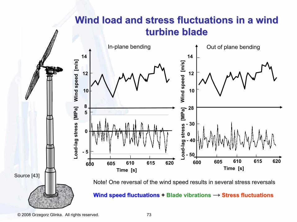
Wind load and stress fluctuations in a wind Wind load and stress fluctuations in a wind turbine bladeturbine blade
Note! One reversal of the wind speed results in several stress reversals
Wind speed fluctuationsWind speed fluctuations
+ + Blade vibrationsBlade vibrations
→→ Stress fluctuationsStress fluctuations
Source [43]
In-plane bending Out of plane bending
Time [s]600 605 610 615 620
Time [s]600 605 610 615 620
Win
d sp
eed
[m/s
]Lo
ad-la
g st
ress
[M
Pa]
- 5
5
0
8
10
12
14
- 400
10
12
14
- 50
- 30
- 28
Win
d sp
eed
[m/s
]Lo
ad-la
g st
ress
[M
Pa]
© 2008 Grzegorz Glinka. All rights reserved. 74
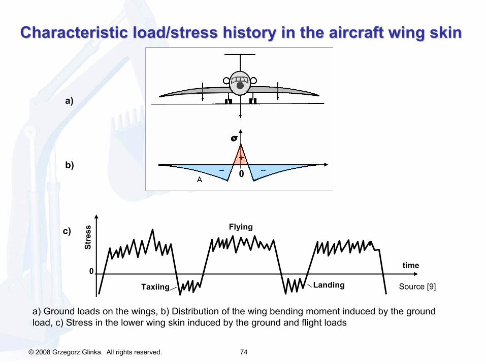
a) Ground loads on the wings, b) Distribution of the wing bending moment induced by the ground load, c) Stress in the lower wing skin induced by the ground and
flight loads
Characteristic load/stress history in the aircraft wing skinCharacteristic load/stress history in the aircraft wing skin
time
Stre
ss
0
Source [9]
σσ
0
a)
LandingTaxiing
Flying
b)
c)
© 2008 Grzegorz Glinka. All rights reserved. 75
maxpeak
σσ
maxpeak
FF
maxpeak
σσ
maxpeak
MM
maxpeak
MM
maxpeak
GG
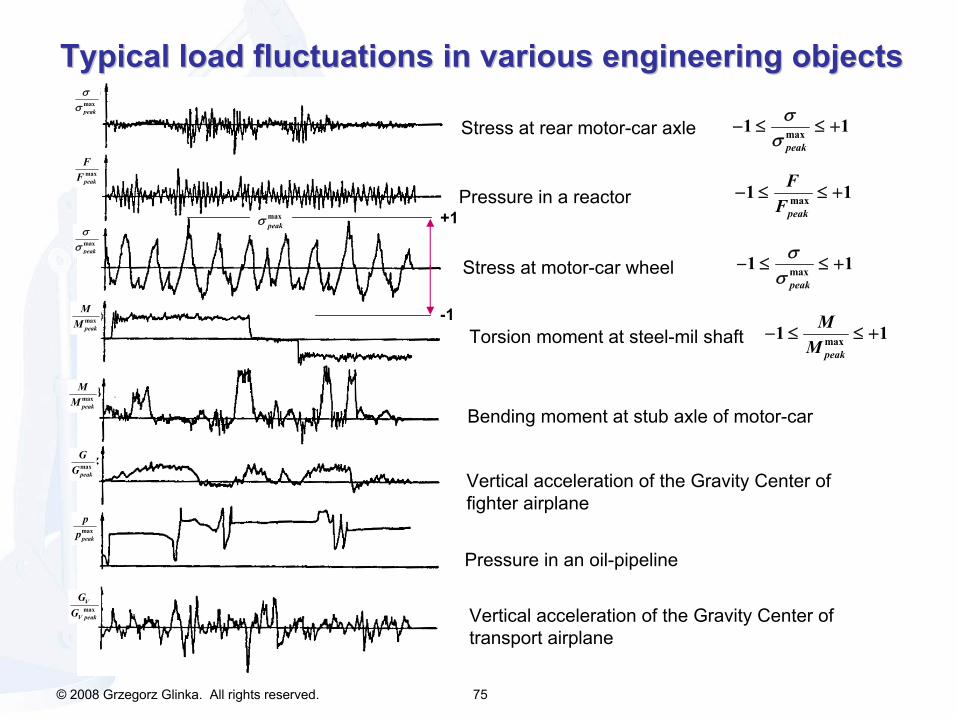
Stress at rear motor-car axle
Pressure in a reactor
Stress at motor-car wheel
Torsion moment at steel-mil shaft
Bending moment at stub axle of motor-car
Vertical acceleration of the Gravity Center of fighter airplane
Pressure in an oil-pipeline
Vertical acceleration of the Gravity Center of transport airplane
maxpeak
pp
maxV
V peak
GG
max1 1peak
σσ
− ≤ ≤ +
max1 1peak
FF
− ≤ ≤ +maxpeakσ +1
-1
max1 1peak
σσ
− ≤ ≤ +
max1 1peak
MM
− ≤ ≤ +
Typical load fluctuations in various engineering objectsTypical load fluctuations in various engineering objects

© 2008 Grzegorz Glinka. All rights reserved. 76
How to get the nominal stress How to get the nominal stress σσnn
from the from the Finite Element method stress data?Finite Element method stress data?
Notched shaft under axial, bending and torsion loadNotched shaft under axial, bending and torsion load
a)
Run each load case separately for an unit load
b) Linearize
the FE stress field for each load case
x3
Fσ22
σ33
r
D
t
x2σ22F
T
Tσ23
MMd
Discrete cross section stress distribution obtained from the FE analysis
d
σ22
0
σnx3 σpeak

© 2008 Grzegorz Glinka. All rights reserved. 77
How to establish the link between the fluctuating load history How to establish the link between the fluctuating load history and the stress distribution, and the stress distribution, σσ((x,yx,y)),,
in the potential crack plane?in the potential crack plane?a) The analytical or FE analysis should be carried out for one characteristic load magnitude, i.e. P=1, Mb
=1, T=1 in order to establish the link between the load and the
stress distribution, kP
, kM
, and kT
such that:
;( , ) ( , ) ( ,( , ) ; ( , ) () , )P M Tbk x yx y x y x yP k x y M k x y Tσ σ τ= ⋅ = ⋅ = ⋅
b) The fluctuating stress distributions corresponding to instantaneous peaks and valleys of the load history are determined by scaling the reference stress distributions kP
(x,y), kM
(x,y), kT
(x,y) by appropriate magnitudes of the load history Pi
, Mb,I
and Ti
such that:
Where: σ(x,y) –
stress distribution in the x-y
plane (crack plane)
kP
(x,y), kM
(x,y), kT
(x,y)
–
reference stress distributions induced by unit loads P=1, Mb
=1, T=1
;,( , ) ; (( , ) ( , ) ( ,) )), ( ,i i ii iP M Tb ik x y P k x y M kx y x y xx y y Tσ σ τ= ⋅ = ⋅ = ⋅
c) In the case of proportional loading
the stress distributions corresponding to peaks and valleys of the load history can be added and the resultant stress distributions can be established. The nominal stress history can be also used as the stress distribution calibration parameter.
;,( , ) ( , )( , ) ii P M b ik x y P kx y x y Mσ += ⋅ ⋅
, ,, , ;( , ) ( , )( , )n P n Mi ii n P n Mx yy k x y k xσ σσ σσ += ⋅ ⋅

© 2008 Grzegorz Glinka. All rights reserved. 78
How to get the resultant stress distributionHow to get the resultant stress distribution
from the from the Finite Element stress data? Finite Element stress data? (Notched shaft under axial, bending load)(Notched shaft under axial, bending load)
x3
Pσ22
σ33
r
D
t
x2Pσ23
MM
dd
σ22
0
σnbx3
Bending
d
x3
σ22
0
σnm
Axiald
σ220
σpeak
Resultant
x3
σ(x3
)

© 2008 Grzegorz Glinka. All rights reserved. 79
Determination of approximate stress distributions in notched Determination of approximate stress distributions in notched bodies bodies (for simultaneous axial and bending load)(for simultaneous axial and bending load)
1 3 2 42 2
1 3 2 42 2
1 1 1 1 1 1 11 1 12 3 2 2 6 22 2 4 2
1 1 1 1 1 1 11 12 3 2 2 6 22 2 4 2t
peax
xxn
kx
x x x x xr r r r
or
K x x x xr r r r
σ
σ σ
σκ
⎡ ⎤⎢ ⎥⎛ ⎞ ⎛ ⎞ ⎛ ⎞ ⎛ ⎞ ⎛ ⎞⎢ ⎥⎜ ⎟ ⎜ ⎟ ⎜ ⎟ ⎜ ⎟ ⎜ ⎟⎜ ⎟ ⎜ ⎟ ⎜ ⎟⎢ ⎥⎜ ⎟ ⎜ ⎟ ⎝ ⎠ ⎝ ⎠ ⎝ ⎠⎝ ⎠ ⎝ ⎠⎢ ⎥⎣ ⎦
⎡⎢ ⎛ ⎞ ⎛ ⎞ ⎛ ⎞ ⎛ ⎞
⎜ ⎟ ⎜ ⎟ ⎜ ⎟ ⎜ ⎟⎜ ⎟ ⎜ ⎟⎜ ⎟ ⎜ ⎟ ⎝ ⎠ ⎝ ⎠⎝ ⎠ ⎝ ⎠⎣
− − − −
− − − −
= + + + + + + + + −
= + + + + + + + + 1 xκ
⎤⎥ ⎛ ⎞⎢ ⎥ ⎜ ⎟⎜ ⎟⎢ ⎥ ⎝ ⎠⎢ ⎥⎦
−
κ → ∞ (for pure axial load) !
κ
= distance to the neutral axis (for pure bending load) !
pe
n
kt
aKσσ
=
x
b)
σn
dn
0
T
r
σpeak
Stre
ss
M
κ
σyy
σxx
2 4
2 4
1 1 12
1 1 12
peakyy
yynt
x x xr r
orK x x x
r r
σκ
σσ κ
σ⎡ ⎤⎛ ⎞ ⎛ ⎞ ⎛ ⎞⎢ ⎥
+⎜ ⎟ ⎜ ⎟ ⎜ ⎟⎢ ⎥⎜ ⎟ ⎜ ⎟ ⎜ ⎟⎝ ⎠ ⎝ ⎠ ⎝ ⎠⎢ ⎥
⎣ ⎦
⎡ ⎤⎛ ⎞ ⎛ ⎞ ⎛ ⎞⎢ ⎥
+⎜ ⎟ ⎜ ⎟ ⎜ ⎟⎢ ⎥⎜ ⎟ ⎜ ⎟ ⎜ ⎟⎝ ⎠ ⎝ ⎠ ⎝ ⎠⎢ ⎥
⎣ ⎦
− −
− −
= + + −
= + + −
Note! Good accuracy for x < 3.5ρ
σnx
dn
0
T
r
σpeak
Stre
ssa) S
σyy
σxx

© 2008 Grzegorz Glinka. All rights reserved. 80
Cyclic nominal stress and corresponding fluctuating stress distrCyclic nominal stress and corresponding fluctuating stress distributionibution
Stre
ss σ
n
time
σn, max
σn, 0
σn, min
x3
d
σ220
Resultant
σ22
(x3
,σn,max
)σ22
(x3
,σn,0
)σ22
(x3
,σn,min
)
© 2008 Grzegorz Glinka. All rights reserved. 81
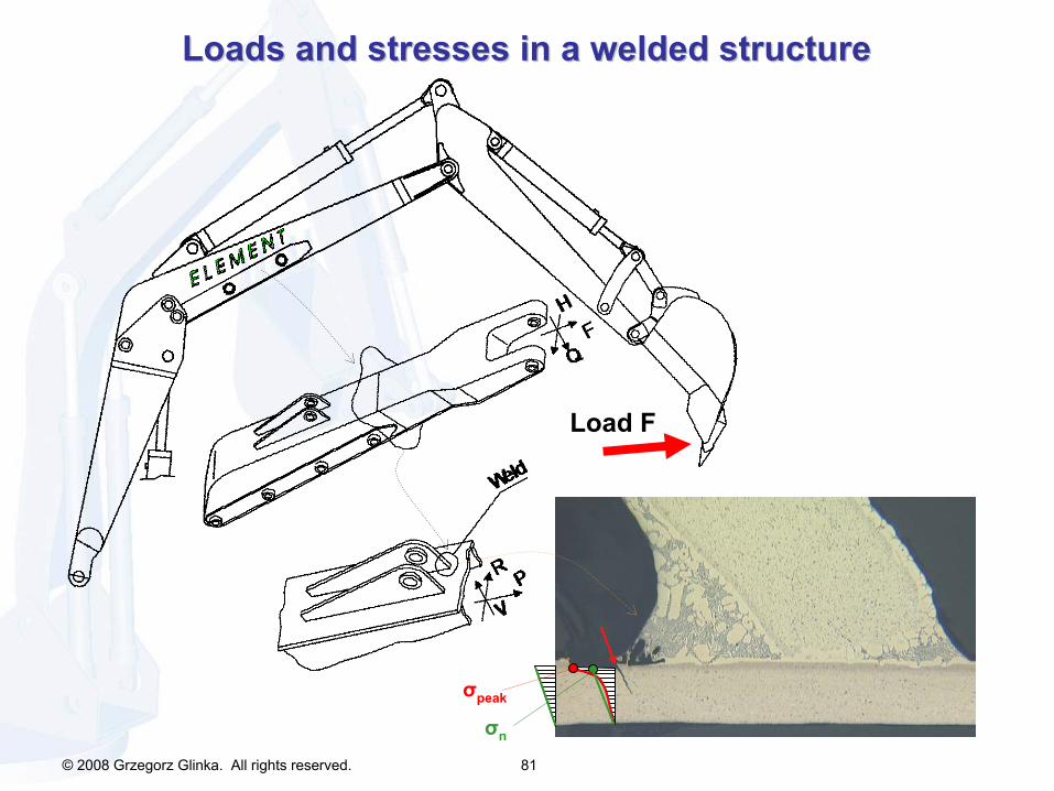
Loads and stresses in a welded structureLoads and stresses in a welded structure
σn
Load F
σpeak

© 2008 Grzegorz Glinka. All rights reserved. 82
Removing material from a clay mine in TennesseeRemoving material from a clay mine in Tennessee

© 2008 Grzegorz Glinka. All rights reserved. 83
Stress history a3799_01 (Right Hand Axle Torque)
–
as recorded
Stress history a3799_01 –
with removed ranges less than 5% of the largest one in the history
The complete Right Hand Axle Torque stress/load historyThe complete Right Hand Axle Torque stress/load history

© 2008 Grzegorz Glinka. All rights reserved. 84
Details of the stress history a3799_c01; visible repeatable workDetails of the stress history a3799_c01; visible repeatable working cycles; ing cycles; ((Right Hand Axle Torque history Right Hand Axle Torque history with removed ranges less than 5% of the largest one in the histowith removed ranges less than 5% of the largest one in the history)ry)
Smax,2
Smax,3
Smax,4Smax,i
Smax,1 Smax,1 =
© 2008 Grzegorz Glinka. All rights reserved. 85
ReliaSoft Weibull++ 7 - www.ReliaSoft.com
Probability - Lognormal
m=4.1795, s=0.1095, r=0.9831 (a3799_01)
Stress, (MPa)
Unr
elia
bilit
y, F
(t)
10.000 100.0000.100
0.500
1.000
5.000
10.000
50.000
99.900
0.100
Probability-Lognormal
Max_01Lognormal-2PRRX SRM MED FMF=87/S=0
Data PointsProbability Line
Grzegorz GlinkaUniversity of Waterloo22/05/20077:24:10 AM
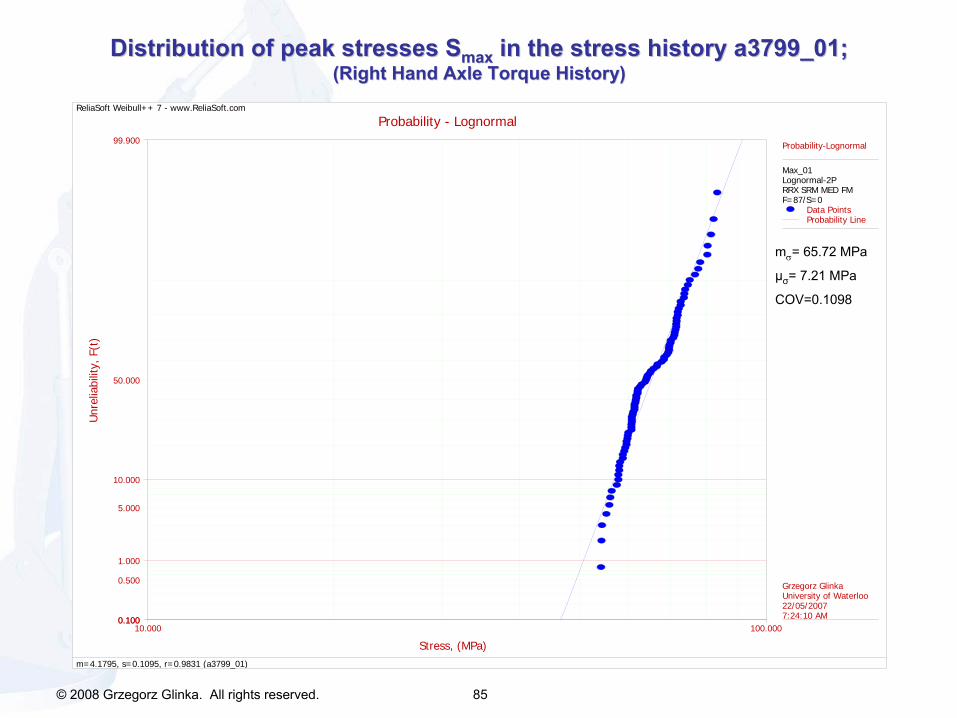
mσ
= 65.72 MPa
μσ
= 7.21 MPa
COV=0.1098
Distribution of peak stresses Distribution of peak stresses SSmaxmax
in the stress history a3799_01; in the stress history a3799_01; ((Right Hand Axle Torque History)Right Hand Axle Torque History)
© 2008 Grzegorz Glinka. All rights reserved. 86
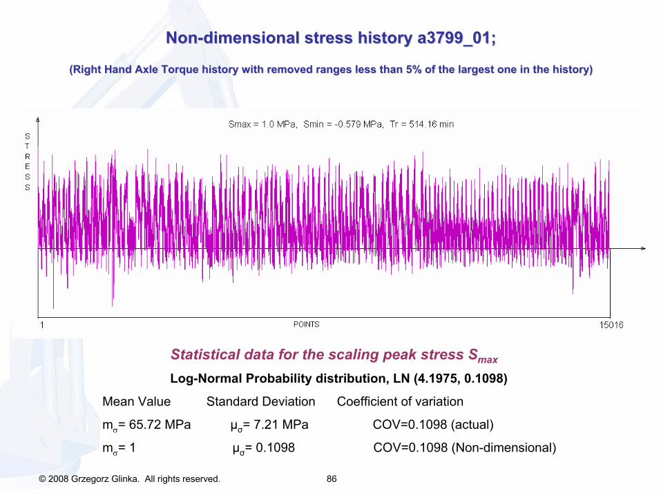
NonNon--dimensional stress history a3799_01; dimensional stress history a3799_01;
((Right Hand Axle Torque history Right Hand Axle Torque history with removed ranges less than 5% of the largest one in the histowith removed ranges less than 5% of the largest one in the history)ry)
Statistical data for the scaling peak stress Smax
Log-Normal Probability distribution, LN (4.1975, 0.1098)
Mean Value Standard Deviation Coefficient of variation
mσ
= 65.72 MPa
μσ
= 7.21 MPa
COV=0.1098 (actual)
mσ
= 1 μσ
= 0.1098 COV=0.1098 (Non-dimensional)

© 2008 Grzegorz Glinka. All rights reserved. 87
The The RainflowRainflow
Cycle Counting ProcedureCycle Counting Procedure

© 2008 Grzegorz Glinka. All rights reserved. 88
Loads and stresses in a structureLoads and stresses in a structure
σn
Load F
σpeak
© 2008 Grzegorz Glinka. All rights reserved. 89
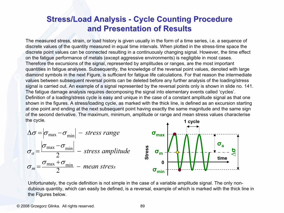
Stress/Load Analysis Stress/Load Analysis --
Cycle Counting ProcedureCycle Counting Procedureand Presentation of Resultsand Presentation of Results
The measured stress, strain, or load history is given usually in
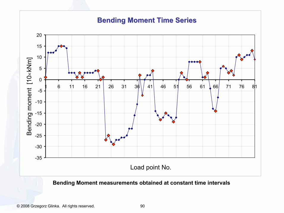
the form of a time series, i.e. a sequence of discrete values of the quantity measured in equal time intervals. When plotted in the stress-time space the discrete point values can be connected resulting in a continuously changing signal. However, the time effect on the fatigue performance of metals (except aggressive environments) is negligible in most cases. Therefore the excursions of the signal, represented by amplitudes or ranges, are the most important quantities in fatigue analyses. Subsequently, the knowledge of the reversal point values, denoted with large diamond symbols in the next Figure, is sufficient for fatigue life calculations. For that reason the intermediate values between subsequent reversal points can be deleted before any further analysis of the loading/stress signal is carried out. An example of a signal represented by the
reversal points only is shown in slide no. 141.The fatigue damage analysis requires decomposing the signal into
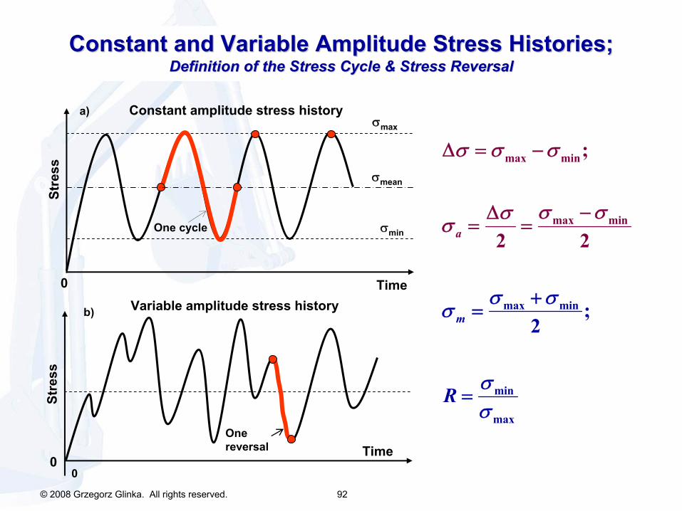
elementary events called ‘cycles’. Definition of a loading/stress cycle is easy and unique in the case of a constant amplitude signal as that one shown in the figures. A stress/loading cycle, as marked with the
thick line, is defined as an excursion starting at one point and ending at the next subsequent point having exactly the same magnitude and the same sign of the second derivative. The maximum, minimum, amplitude or range and mean stress values characterise the cycle.
Unfortunately, the cycle definition is not simple in the case of
a variable amplitude signal. The only non-
dubious quantity, which can easily be defined, is a reversal, example of which is marked with the thick line in the Figures below.
max min
max min
max min
2
2
a
m s
stress range
stress amplitude
mean stres
σ σ σ
σ σσ
σ σσ
Δ = − −
−= −
+= −
σmax
σmin
timeStre
ssσa
1 cycle
0
σm ∆σ
© 2008 Grzegorz Glinka. All rights reserved. 90
Bending Moment Time SeriesBending Moment Time Series
-35
-30
-25
-20
-15
-10
-5
0
5
10
15
20
1 6 11 16 21 26 31 36 41 46 51 56 61 66 71 76 81
Load point No.
Ben
ding
mom
ent
[10×
kNm
]
Bending Moment measurements obtained at constant time intervals

© 2008 Grzegorz Glinka. All rights reserved. 91
Bending Moment History Bending Moment History --
Peaks and ValleysPeaks and Valleys
-35
-30
-25
-20
-15
-10
-5
0
5
10
15
20
1 3 5 7 9 11 13 15 17 19 21 23 25 27 29
Load point No.
Ben
ding
mom
ent v
alue
[10×
kNm
]
Bending Moment signal represented by the reversal point values
© 2008 Grzegorz Glinka. All rights reserved. 92
Constant and Variable Amplitude Stress Histories;Constant and Variable Amplitude Stress Histories; Definition of the Stress Cycle & Stress ReversalDefinition of the Stress Cycle & Stress Reversal
max min
max min
max min
min
max
;
2 2
;2
a
m
R
σ σσ
σ
σ σ σ
σσ
σ
σσ
+=
=
Δ = −
−Δ= =
Stre
ss
Time0
Variable amplitude stress history
One reversal
b)
0
One cycle
σmean
σmax
σmin
Stre
ss
Time0
Constant amplitude stress historya)

© 2008 Grzegorz Glinka. All rights reserved. 93
Stress Reversals and Stress Cycles in a Variable Stress Reversals and Stress Cycles in a Variable Amplitude Stress HistoryAmplitude Stress History
The reversalreversal
is simply an excursion between two-consecutive reversal points, i.e. an excursion between subsequent peak and valley
or valley and peak.
In recent years the rainflowrainflow
cycle counting method has been accepted world-wide as the most appropriate for extracting stress/load cycles for fatigue analyses. The rainflowrainflow
cycle is defined as a stress excursion, which when applied to a deformable material, will generate a closed stressstress--strain hysteresis loopstrain hysteresis loop. It is believed that the surface area of the stress-strain hysteresis loop represents the amount of damage induced by given cycle. An example of a short stress history and its rainflowrainflow
counted cyclescounted cycles
content is shown in the following Figure.

© 2008 Grzegorz Glinka. All rights reserved. 94
A rainflow
counted cycle
is identified when any two adjacent reversals in the stress history satisfy the following relation:
1 1i i i iABS ABSσ σ σ σ− +− ≤ −
Stre
ss
Time
Stress history Rainflow
counted cycles
σi-1
σi-2
σi+1
σi
σi+20
Stress History and the Stress History and the ““RainflowRainflow””
Counted CyclesCounted Cycles
© 2008 Grzegorz Glinka. All rights reserved. 95
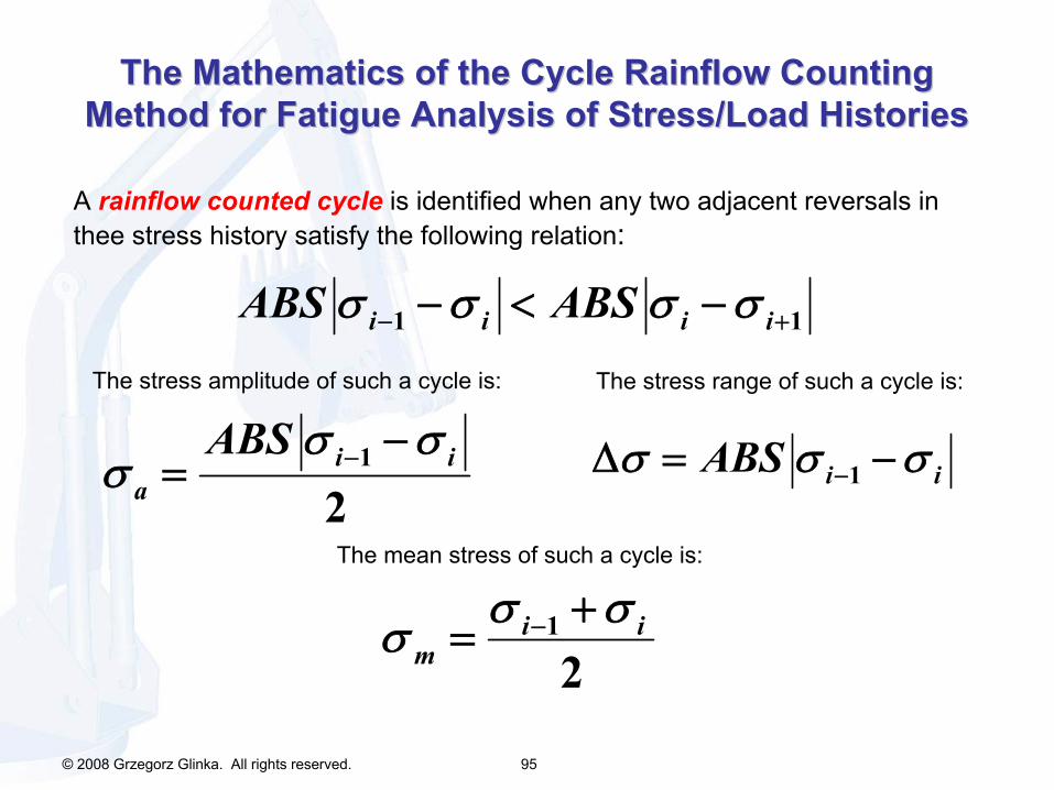
A rainflow
counted cycle
is identified when any two adjacent reversals in thee stress history satisfy the following relation:
1 1i i i iABS ABSσ σ σ σ− +− < −
The stress amplitude of such a cycle is:
1
2i i
a
ABS σ σσ − −
=
The stress range of such a cycle is:
1i iABSσ σ σ−Δ = −
The mean stress of such a cycle is:
1
2i i
mσ σσ − +
=
The Mathematics of the Cycle The Mathematics of the Cycle RainflowRainflow
Counting Counting Method for Fatigue Analysis of Stress/Load HistoriesMethod for Fatigue Analysis of Stress/Load Histories

© 2008 Grzegorz Glinka. All rights reserved. 96
The ASTM The ASTM rrainflowainflow
cycle counting procedurecycle counting procedure
--
exampleexample
Determine stress ranges, ΔSi
, and corresponding mean stresses, Smi
for the stress history given below. Use the ASTM ‘rainflow’
counting procedure.
Si
= 0, 4, 1, 3, 2, 6, -2, 5, 1, 4, 2, 3, -3, 1, -2
(units: MPa·102)
0 1 2 3 4 5 6 7 8 9 10 11 12 13 14
1
2
3
4
5
6
0
-1
-2
-3
Stre
ss S
i(M
Pa·1
02)
Reversing point number, i

© 2008 Grzegorz Glinka. All rights reserved. 97
Reversal point No.
RainflowRainflow
cycle counting cycle counting ––
The The Direct Direct MMethod:ethod:1. Find the absolute maximum revesal point; 1. Find the absolute maximum revesal point;
2. Add the absolute maximum at the end of the history, 2. Add the absolute maximum at the end of the history, i.e. make it to be the last reversing point in the history;
3. Start counting form the reversal no. 3 (always); 3. Start counting form the reversal no. 3 (always);
Stress History
-3
-2
-1
0
1
2
3
4
5
6
0 1 2 3 4 5 6 7 8 9 10 11 12 13 14Stre
ss (M
Pa)x
102
Absolute maximum
-3-2-101
23
456
0 1 2 3 4 5 6 7 8 9 10 11 12 13 14
Stre
ss (M
Pa)x
102
Starting point
© 2008 Grzegorz Glinka. All rights reserved. 98
-3-2-10
1
23
456
0 1 2 3 4 5 6 7 8 9 10 11 12 13 14
Stre
ss (M
Pa)x
102
-3-2-101
23
456
0 1 2 3 4 5 6 7 8 9 10 11 12 13 14
Stre
ss (M
Pa)x
102
Starting point
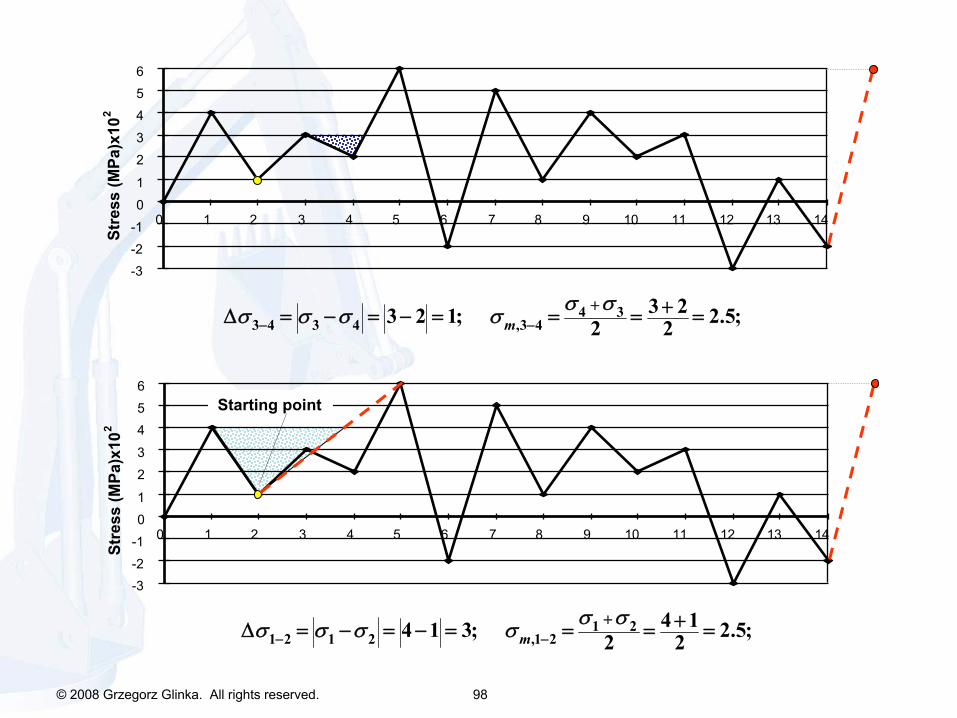
4 33 4 3 4 ,3 4
3 23 2 1; 2.5;2 2mσ σσ σ σ σ− −
+ +Δ = − = − = = = =
1 21 2 1 2 ,1 2
4 14 1 3; 2.5;2 2mσ σσ σ σ σ− −
+ +Δ = − = − = = = =
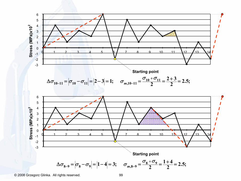
© 2008 Grzegorz Glinka. All rights reserved. 99
10 1110 11 10 11 ,10 11
2 32 3 1; 2.5;2 2mσ σσ σ σ σ− −
+ +Δ = − = − = = = =
8 98 9 8 9 ,8 9
1 41 4 3; 2.5;2 2mσ σσ σ σ σ− −
+ +Δ = − = − = = = =
-3-2-101
23
456
0 1 2 3 4 5 6 7 8 9 10 11 12 13 14
Stre
ss (M
Pa)x
102
Starting point
-3-2-101
23
456
0 1 2 3 4 5 6 7 8 9 10 11 12 13 14
Stre
ss (M
Pa)x
102
Starting point

© 2008 Grzegorz Glinka. All rights reserved. 100
-3-2-101
23
456
0 1 2 3 4 5 6 7 8 9 10 11 12 13 14
Stre
ss (M
Pa)x
102
Starting point
7676 7 6 ,6 7
2 52 5 7; 1.5;2 2mσ σσ σ σ σ− −
+ − +Δ = − = − − = = = =
-3-2-101
23
456
0 1 2 3 4 5 6 7 8 9 10 11 12 13 14
Stre
ss (M
Pa)x
102
Starting point
13 1413 14 13 14 ,13 14
1 21 ( 2) 3; 0.5;2 2mσ σσ σ σ σ− −
+ −Δ = − = − − = = = = −

© 2008 Grzegorz Glinka. All rights reserved. 101
-3-2-101
23
456
0 1 2 3 4 5 6 7 8 9 10 11 12 13 14
Stre
ss (M
Pa)x
102
Starting point
5 1255 12 12 ,5 12
6 36 ( 3) 9; 1.5;2 2mσ σσ σ σ σ− −
+ −Δ = − = − − = = = =
Cycles counted Cycles counted ––
Direct methodDirect method1. ∆σ3-
4 =1; σm,3-
4 = 2.5; 2. ∆σ1-
2 =3; σm,1-
2 = 2.5; 3. ∆σ10-
11
=1; σm,10-
11
= 2.5; 4. ∆σ8-
9 =3; σm,8-
9 = 2.5; 5. ∆σ6-
7 =7; σm,6-
7 = 1.5; 6. ∆σ13-
14 =3; σm,13-
14
=-0.5; 7. ∆σ5-
12 =9; σm,5-
12 = 1.5;

© 2008 Grzegorz Glinka. All rights reserved. 102
Extracted rainflow cycles, Extracted rainflow cycles, ΔσΔσ--
ΔσΔσmm

© 2008 Grzegorz Glinka. All rights reserved. 103
EExtracted rainflow cyclesxtracted rainflow cycles
––
the the ΔσΔσ--
ΔσΔσmm
matrixmatrix
Total number of cycles, N=854
Δσ/σm -32 -22 -13 -3.2 6.44 16.1 25.7 35.3 45 54 64.1 73.7 83.3 92.9 103 112 122 131 141 151 Δσ298.8 0 0 0 0 0 0 0 0 0 1 0 0 0 0 0 0 0 0 0 0 1283.9 0 0 0 0 0 0 0 0 0 0 0 0 0 0 0 0 0 0 0 0 0268.9 0 0 0 0 0 0 0 0 1 0 0 0 0 0 0 0 0 0 0 0 1254 0 0 0 0 0 0 0 0 0 1 0 0 0 0 0 0 0 0 0 0 1239 0 0 0 0 0 0 0 1 2 2 0 0 0 0 0 0 0 0 0 0 5
224.1 0 0 0 0 0 0 0 0 2 2 1 0 0 0 0 0 0 0 0 0 5209.2 0 0 0 0 0 0 0 3 4 5 2 0 0 0 0 0 0 0 0 0 14194.2 0 0 0 0 0 1 0 1 7 2 0 0 0 0 0 0 0 0 0 0 11179.3 0 0 0 0 0 0 1 0 4 4 0 0 0 0 0 0 0 0 0 0 9164.3 0 0 0 0 1 0 0 0 3 1 0 0 0 0 0 0 0 0 0 0 5149.4 0 0 0 0 0 0 1 0 0 0 0 2 1 0 0 0 0 0 0 0 4134.5 0 0 0 0 0 0 0 0 0 0 0 4 1 1 0 0 0 0 0 0 6119.5 0 1 1 0 0 0 0 0 0 0 3 1 5 1 2 0 0 0 0 0 14104.6 0 0 1 2 1 0 0 0 0 2 4 3 7 3 2 1 2 1 0 0 2989.64 0 1 2 3 7 2 0 0 0 1 2 8 10 7 5 6 2 1 0 0 5774.7 1 1 3 4 3 5 0 1 2 2 10 18 23 20 17 11 4 1 0 0 126
59.76 2 1 5 7 4 1 4 5 1 2 11 20 34 31 31 28 9 7 1 1 20544.82 1 6 9 7 9 7 10 3 3 8 15 37 49 64 62 41 16 11 2 1 36129.88 0 0 0 0 0 0 0 0 0 0 0 0 0 0 0 0 0 0 0 0 014.94 0 0 0 0 0 0 0 0 0 0 0 0 0 0 0 0 0 0 0 0 0
854
Mean stress, σm
Stre
ss ra
nge,
Δσ
© 2008 Grzegorz Glinka. All rights reserved. 104
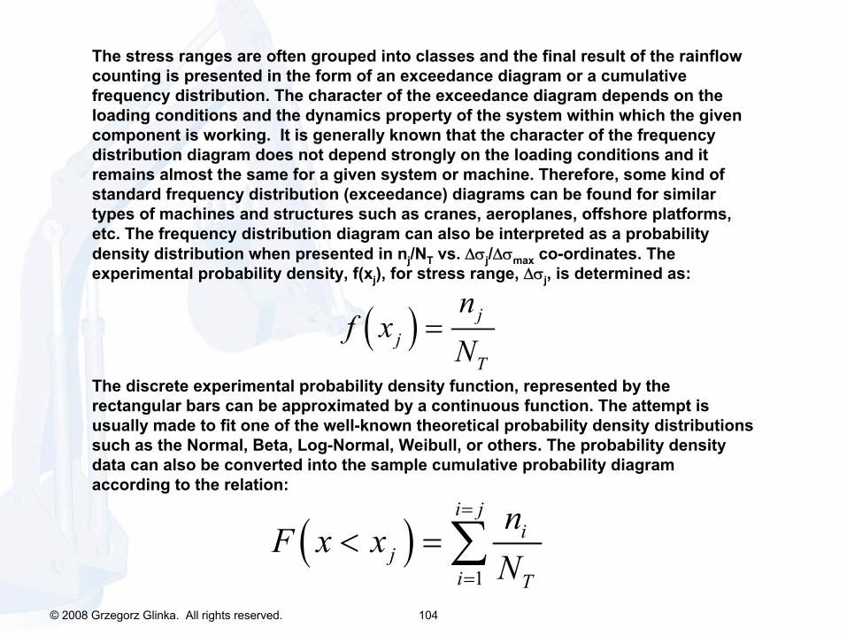
The stress ranges are often grouped into classes and the final result of the rainflow
counting is presented in the form of an exceedance
diagram or a cumulative frequency distribution. The character of the exceedance
diagram depends on the loading conditions and the dynamics property of the system within which the given component is working. It is generally known that the character of the frequency distribution diagram does not depend strongly on the loading conditions and it remains almost the same for a given system or machine. Therefore, some kind of standard frequency distribution (exceedance) diagrams can be found for similar types of machines and structures such as cranes, aeroplanes, offshore platforms, etc. The frequency distribution diagram can also be interpreted as a probability density distribution when presented in nj
/NT
vs. Δσj
/Δσmax
co-ordinates. The experimental probability density, f(xj
), for stress range, Δσj
, is determined as:
The discrete experimental probability density function, represented by the rectangular bars can be approximated by a continuous function. The attempt is usually made to fit one of the well-known theoretical probability density distributions such as the Normal, Beta, Log-Normal, Weibull, or others. The probability density data can also be converted into the sample cumulative probability diagram according to the relation:
( ) jj
T
nf x
N=
( )1
i ji
ji T
nF x x
N
=
=
< = ∑
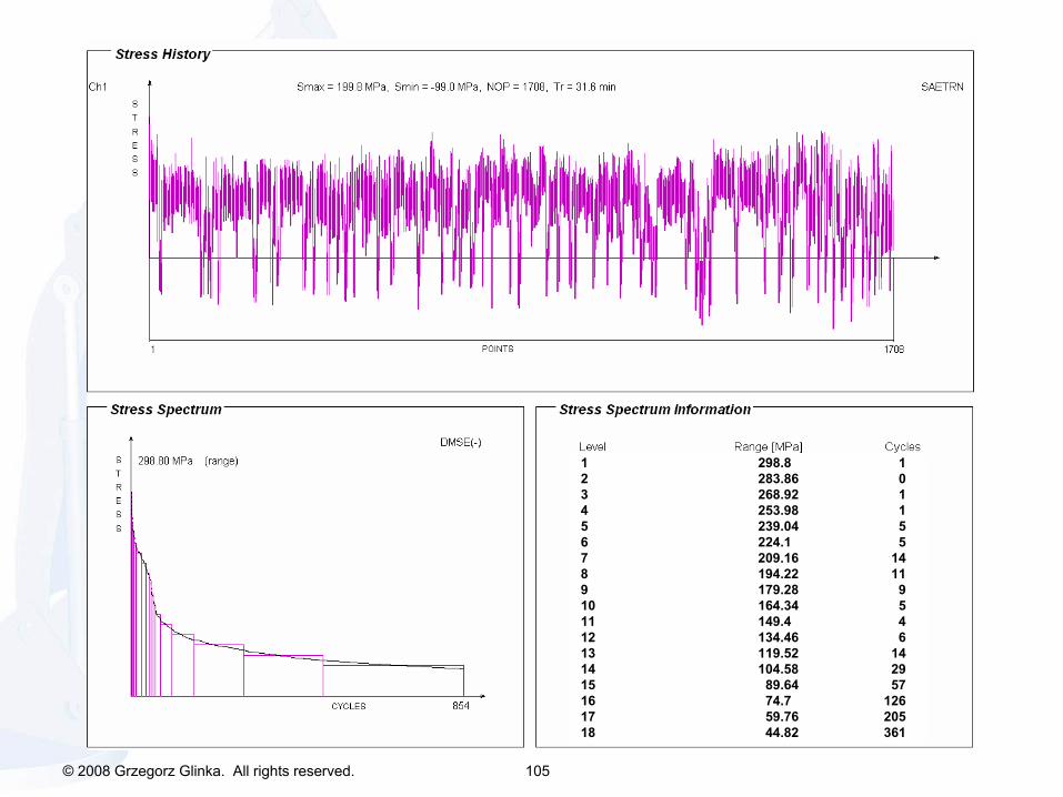
© 2008 Grzegorz Glinka. All rights reserved. 105
1 298.8 12 283.86 03 268.92 14 253.98 15 239.04 56 224.1 57 209.16 148 194.22 119 179.28 910 164.34 511 149.4 412 134.46 613 119.52 1414 104.58 2915 89.64 5716 74.7 12617 59.76 20518 44.82 361
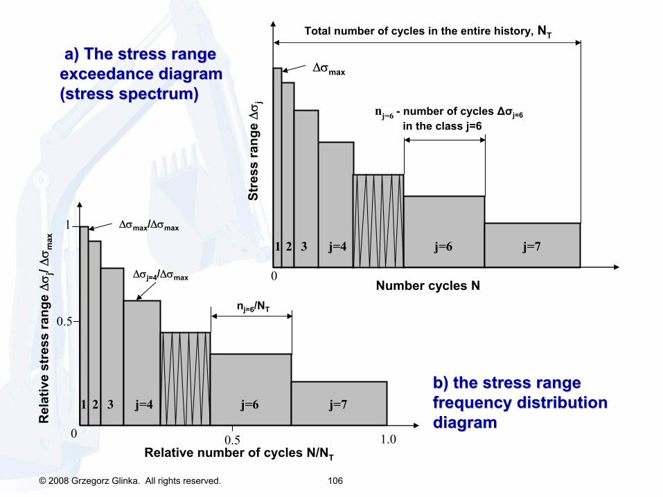
© 2008 Grzegorz Glinka. All rights reserved. 106
b) the stress range b) the stress range frequency distribution frequency distribution diagramdiagram
Number cycles N
Stre
ss ra
nge
Δσ j
j=7j=6
nj=6
-
number of cycles Δσj=6in the class j=6
Total number of cycles in the entire history,
NT
Δσmax
Rel
ativ
e st
ress
rang
e Δ
σ j/ Δ
σ max
Relative number of cycles N/NT
0
j=7j=6j=4321
nj=6
/NT
Δσmax
/Δσmax1
Δσj=4
/Δσmax
0.5 1.0
0.5
0
j=4321
a) The stress range a) The stress range exceedanceexceedance
diagram diagram (stress spectrum)(stress spectrum)
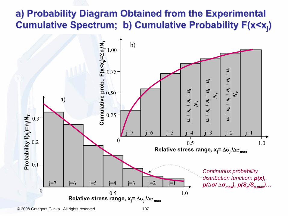
© 2008 Grzegorz Glinka. All rights reserved. 107
a) Probability Diagram Obtained from the Experimental a) Probability Diagram Obtained from the Experimental Cumulative Spectrum; b) Cumulative Probability Cumulative Spectrum; b) Cumulative Probability F(xF(x<<xxjj
))
Relative stress range, xj
= Δσj /Δσmax
Prob
abili
ty f(
x j)=
n j/N
T
0j=7 j=6 j=4
0.3
0.5 1.0
0.1
0.2
j=5 j=3 j=2 j=1
a)
0j=7 j=6 j=4
0.5 1.0
0.25
j=5 j=3 j=2 j=1
0.50
0.75
1.00
nn
nn
nn
NT
76
54
32
++
++
+
nn
nn
nNT
76
54
3+
++
+
nn
nn
NT
76
54
++
+
Relative stress range, xj
= Δσj /Δσmax
Cum
ulat
ive
prob
., F(
x<x j
)=Σn
j/NT b)
Continuous probability distribution function: p(x), p(∆σ/ ∆σmax
), p(Sa
/Sa,max
)…
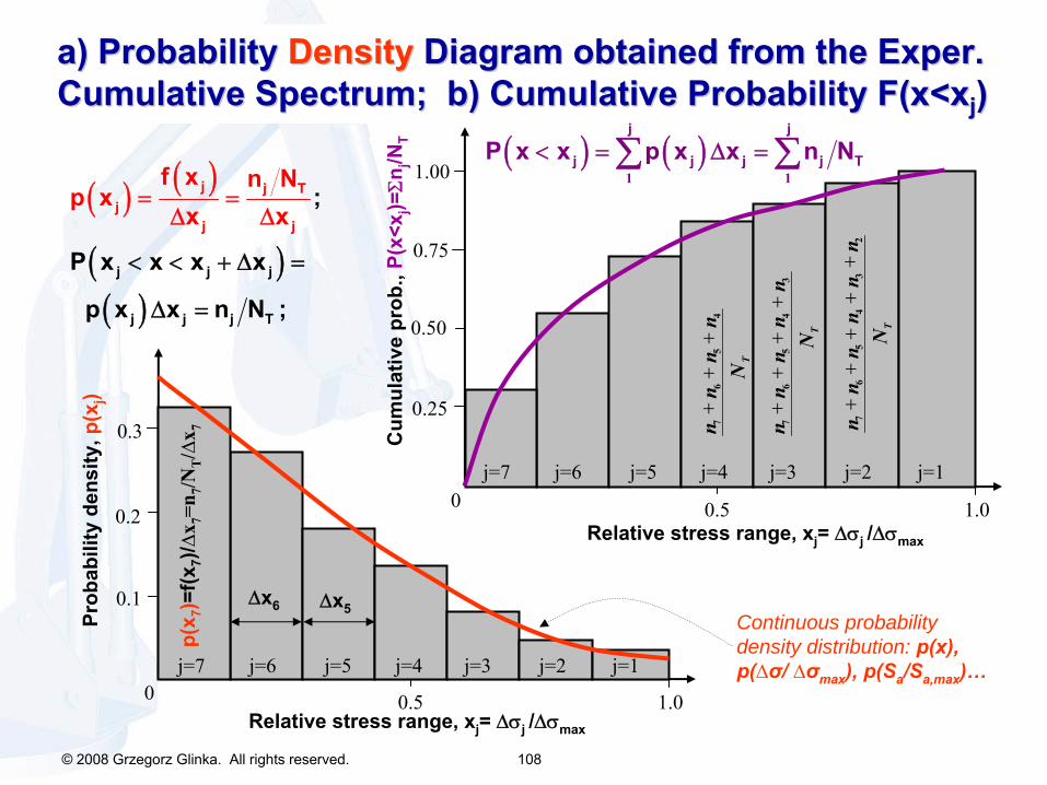
© 2008 Grzegorz Glinka. All rights reserved. 108
a) Probability a) Probability DensityDensity
Diagram obtained from the Diagram obtained from the ExperExper. . Cumulative Spectrum; b) Cumulative Probability Cumulative Spectrum; b) Cumulative Probability F(xF(x<<xxjj
))
Continuous probability density distribution: p(x), p(∆σ/ ∆σmax
), p(Sa
/Sa,max
)…
( ) ( )
( )( )
<
= =Δ
< + Δ =
Δ =
Δj j T
j j j
j j j T
jj j
f x n Np ;
P x x x x
p x x
x
n
x
N
x
;
0j=7 j=6 j=4
0.5 1.0
0.25
j=5 j=3 j=2 j=1
0.50
0.75
1.00
nn
nn
nn
NT
76
54
32
++
++
+
nn
nn
nNT
76
54
3+
++
+
nn
nn
NT
76
54
++
+
Relative stress range, xj
= Δσj /Δσmax
Cum
ulat
ive
prob
., P(
x<x j
)=Σn
j/NT ( ) ( )
1 1
< = Δ =∑ ∑j j
j j j j TP x x p x x n N
Relative stress range, xj
= Δσj /Δσmax
Prob
abili
ty d
ensi
ty, p
(xj)
0j=7 j=6 j=4
0.3
0.5 1.0
0.1
0.2
j=5 j=3 j=2 j=1
Δx6 Δx5
p(x 7
)=f(x
7)/∆x
7=n 7/N
T/∆
x 7

© 2008 Grzegorz Glinka. All rights reserved. 109
The use of the probability density distributionThe use of the probability density distribution
Given are:
The maximum stress amplitude, Sa,max
and the total number of cycles in the spectrum NT
and the probability density function p(Sa
/Sa,max
) = p(x);
The task
of the analyst is to determine the number of applications (cycles) nj
of
stress amplitudes within
the interval (Sa,j
< Sa
< Sa,j+1
);
Find
how many cycles nj with amplitudes Sa,j
< Sa
< Sa,j+1
are to be found out in the total population
of NT
load cycles to be applied.
xj
=Sa,j
/Sa,max
and
xj+1
=Sa,j+1
/Sa,max.
1+
= ⋅ ∫j
j
x
j Tx
n N p(x)dx
Number of cycles in the class j:
12
+ += a,j a,ja,j
S SS
Average stress in the class j:

© 2008 Grzegorz Glinka. All rights reserved. 110
Various Various LoadLoadinging
SpectraSpectraa) constant amplitude, b) mixed spectrum, c) Gaussian normal spectrum, d-
e) mixed spectra
Relative number of cycles, Ni
/NTotal
Rel
ativ
e st
ress
am
plitu
de, σ
a,i/
σ max
a
σ(t)
σ(t)
d
f
σ(t)
t
t
t10-6 10-5 10-4 10-3 10-2 10-1 10
0.2
0.2
0.2
0.2
1.0
0
a
bc
d
e
f

© 2008 Grzegorz Glinka. All rights reserved. 111
Stre
ss M
PaS
tress
am
p. M
Pa
Stress signal
–
Time Domain RepresentationTime Domain Representation
Stress signal
–
Frequency Domain RepresentationFrequency Domain Representation
Sequence of peaks and valleys
Amplitudes associated with certain frequencies
Courtesy of D. Socie, Univ. of Illinois
Ways of representing the stress signalWays of representing the stress signal

© 2008 Grzegorz Glinka. All rights reserved. 112
A Frequency Domain approach to fatigue A Frequency Domain approach to fatigue analysis of random cyclic stress processes analysis of random cyclic stress processes In the case of vibration induced stresses and strains the determination of the stress-
or strain-time history as discussed earlier is rather difficult and very often the stress signal/process can not be determined in a deterministic form.
Therefore concepts taken from random process theory, such as the
power spectral density (PSD),
root mean square (RMS)
and the Fourier transform
analysis are used to characterize random load and stress histories.
The task of the analyst is determine the most probable stress spectrum or the probability density distribution of stress amplitudes of the analysed object knowing the statistical properties (PSD, RMS,
etc.) of the stress process at the critical location.
The stress spectrum determined in the form of discrete classes of stress amplitudes or in the form of a probability density distribution is subsequently used for the determination of cumulative fatigue damage and fatigue durability.
Therefore some elements of the random process theory need to be reviewed including the physical interpretation of basic parameters used for the characterisation of a random process such as the stress fluctuations induced by a random excitation signal.

© 2008 Grzegorz Glinka. All rights reserved. 113
Load time Load time historyhistory
Structural Structural modelmodel
General fatigue analysis proceduresGeneral fatigue analysis procedures
Stress time Stress time historyhistory
Stress CyclesStress CyclesMiner Miner
fatigue fatigue damagedamage
FATIGUE FATIGUE LIFELIFE
Acceleration Acceleration PSDPSD
Transfer Transfer functionfunction
( TIME DOMAIN )( TIME DOMAIN )
( FREQUENCY DOMAIN )( FREQUENCY DOMAIN )
Stress Stress PSDPSD
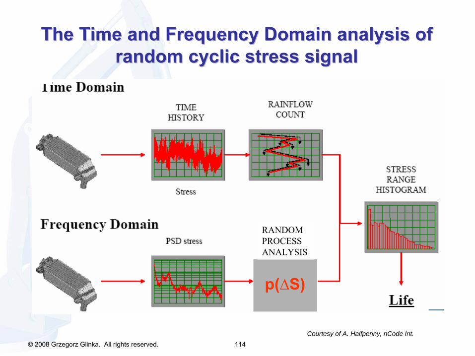
© 2008 Grzegorz Glinka. All rights reserved. 114
RANDOM PROCESS ANALYSIS
p(∆S)
The Time and Frequency Domain analysis of The Time and Frequency Domain analysis of random cyclic stress signal random cyclic stress signal
Courtesy of A. Halfpenny, nCode Int.
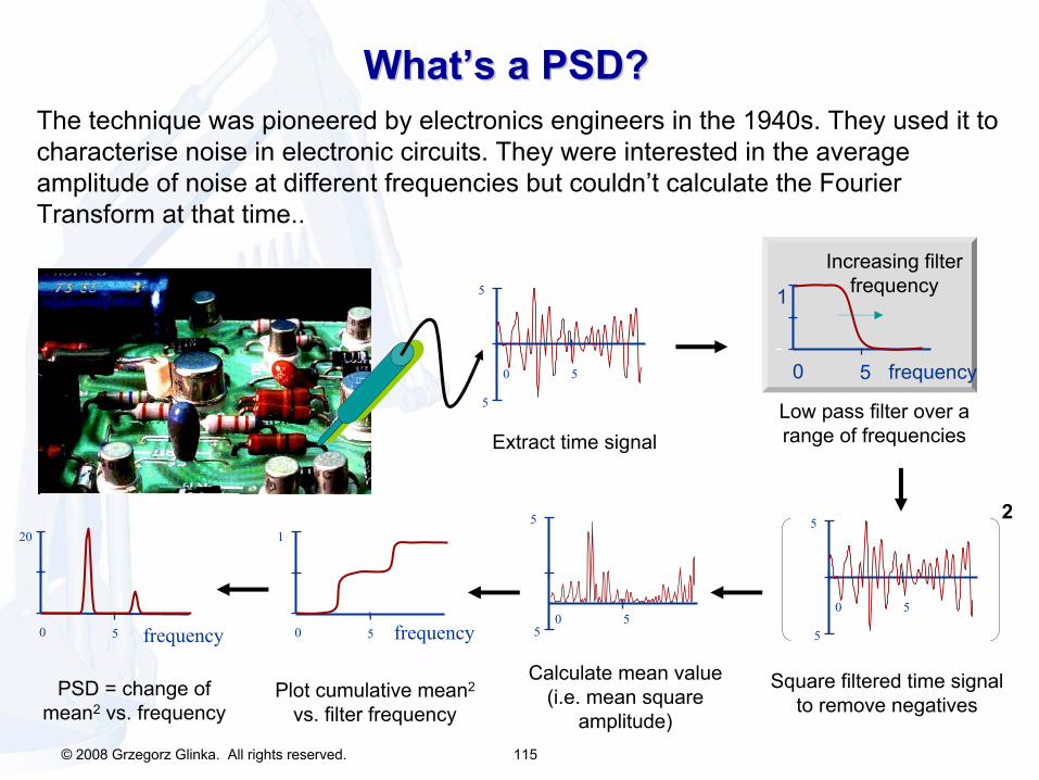
© 2008 Grzegorz Glinka. All rights reserved. 115
The technique was pioneered by electronics engineers in the 1940s. They used it to characterise noise in electronic circuits. They were interested in the average amplitude of noise at different frequencies but couldn’t calculate the Fourier Transform at that time..
0 5
5
5
Extract time signal
0 5
1
Increasing filter frequency
frequency
Low pass filter over a range of frequencies
0 5
5
52
Square filtered time signal to remove negatives
0 55
5
Calculate mean value (i.e. mean square
amplitude)
0 5
20
frequency
PSD = change of mean2
vs. frequency
0 5
1
frequency
Plot cumulative mean2
vs. filter frequency
WhatWhat’’s a PSD?s a PSD?
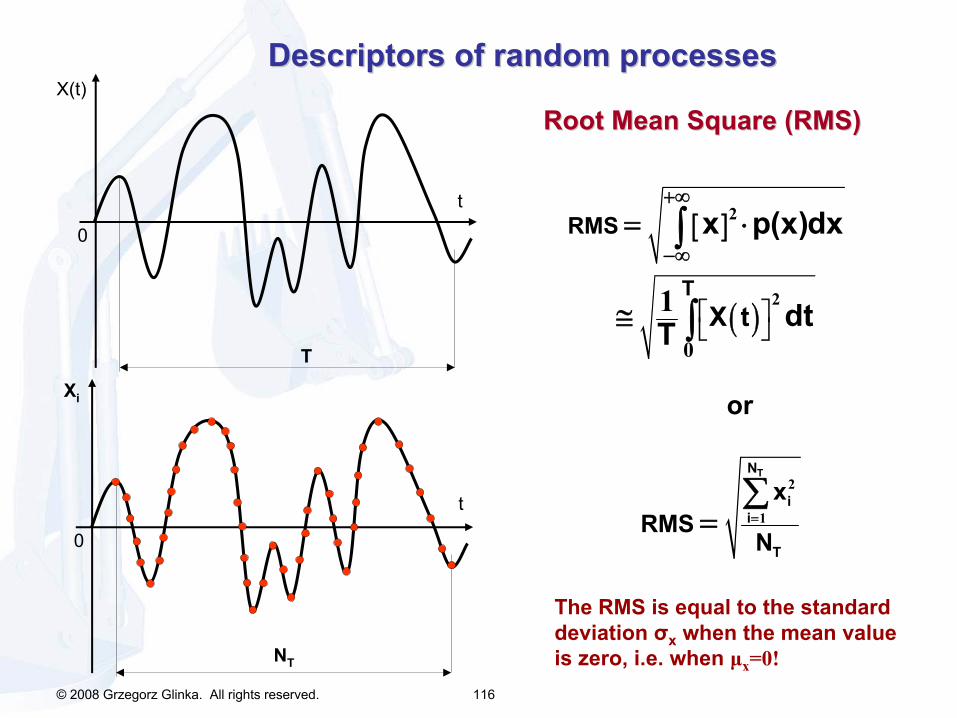
© 2008 Grzegorz Glinka. All rights reserved. 116
Descriptors of random processesDescriptors of random processes
t
X(t)
0
T
Root Mean Square (RMS)Root Mean Square (RMS)
[ ]
( )
2
2
0
1 T
RMS
X t
x p(x)dx
dtT
+∞
−∞
⎡ ⎤⎣ ⎦
= ⋅
≅
∫
∫
2
1
TN
ii
T
xRMS
N==∑
or
0
t
Xi
NT
The RMS is equal to the standard deviation σx
when the mean value is zero, i.e. when μx
=0!
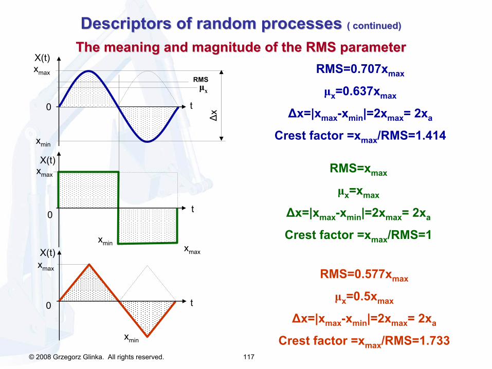
© 2008 Grzegorz Glinka. All rights reserved. 117
Descriptors of random processes Descriptors of random processes ( continued)( continued)
The meaning and magnitude of the RMS parameterThe meaning and magnitude of the RMS parameter
Δx
xmax
X(t)
xmax
X(t)
0
0
xmax
X(t)
0
t
t
t
RMSμx
xmin
xmax
xmin
xmin
RMS=0.707xmax
μx
=0.637xmax
Δx=|xmax
-xmin
|=2xmax
= 2xa
Crest factor =xmax
/RMS=1.414
RMS=xmax
μx
=xmax
Δx=|xmax
-xmin
|=2xmax
= 2xa
Crest factor =xmax
/RMS=1
RMS=0.577xmax
μx
=0.5xmax
Δx=|xmax
-xmin
|=2xmax
= 2xa
Crest factor =xmax
/RMS=1.733
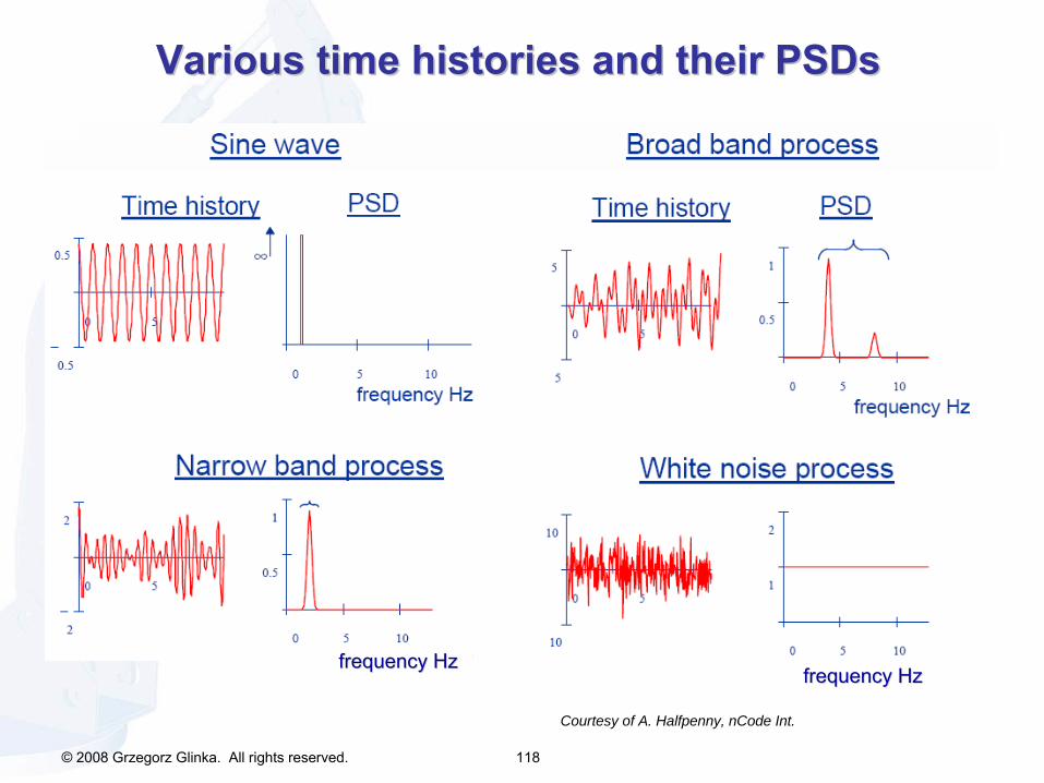
© 2008 Grzegorz Glinka. All rights reserved. 118
frequency Hzfrequency Hzfrequency Hzfrequency Hz
Various time histories and their Various time histories and their PSDsPSDs
Courtesy of A. Halfpenny, nCode Int.

© 2008 Grzegorz Glinka. All rights reserved. 119
The NatThe Natuure of Frequency Analysis re of Frequency Analysis –– the light spectrum analogythe light spectrum analogy
Courtesy of A. Halfpenny, nCode Int.
•
Fourier Transform
is the mathematical equivalent
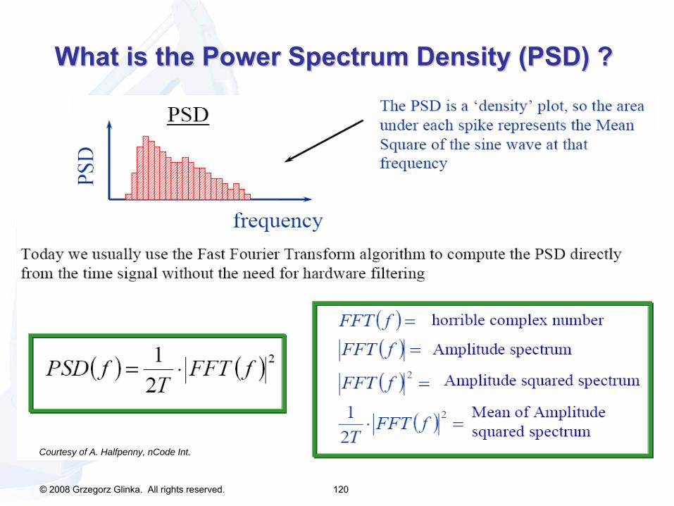
© 2008 Grzegorz Glinka. All rights reserved. 120
What is What is thethe
Power Spectrum Density (PSD) ? Power Spectrum Density (PSD) ?
Courtesy of A. Halfpenny, nCode Int.

© 2008 Grzegorz Glinka. All rights reserved. 121
TheThe
Fourier TransformFourier TransformAfter replacing the ‘n/T’
term by frequency ‘f’
the Fourier transform equations can be written as:
( ) ( )+∞
− ⋅ ⋅ ⋅
−∞
= ∫ 22 i f tX f X t e dtπ ( ) ( )+∞
− ⋅ ⋅ ⋅= ∫ 2
0
2 i f tX t X f e dfπ
Fourier Transform
from time to frequency domain:
Inverse Fourier Transform
from frequency to time domain:
( ) ( )⎛ ⎞
− ⋅ ⋅⎜ ⎟⎝ ⎠= ⋅∑
22 T
ni kN
n kkT
TX f X t eN
π
( ) ( )⎛ ⎞
− ⋅ ⋅⎜ ⎟⎝ ⎠= ⋅∑
21 T
ni kN
k kn
X t X t eT
π
ContinuousContinuous
process
Discrete processDiscrete process
Inverse Fourier TransformInverse Fourier Transform
Fourier TransformFourier Transform
Time Time domaindomain
Frequency Frequency domaindomain

© 2008 Grzegorz Glinka. All rights reserved. 122
The Number of CyclesThe Number of Cycles
t
Stre
ss
0
1 sec
P
0+
Upward zero crossing, 0+
Peak P
( )( )
EIF
E P
+
= =0 3
5
SO Rice, 1954
E[0+]
Expected number of upward zero crossing 0+
E[P]
Expected number of peaks
( )= ⋅ ⋅ δ∑ nnm f G f f
Number of upward zero crossing: ( ) 0
2
mE 0
m+ =
Number of peaks: ( ) 4
2
mE P
m=
The nth
moment area under PSD:
Frequency f, [Hz]
G(f)
, (St
ress
2 )/H
z
fk
Gk(f
)
δf
Irregularity factor

© 2008 Grzegorz Glinka. All rights reserved. 123
The Cycle Ranges The Cycle Ranges –– narrow band narrow band processprocess
JS Bendat, 1964 Courtesy of A. Halfpenny, nCode Int.
( )Δ
−ΔΔ =
2
08
04
SmSp S e
m
N(∆S)∆S
(∆S)2
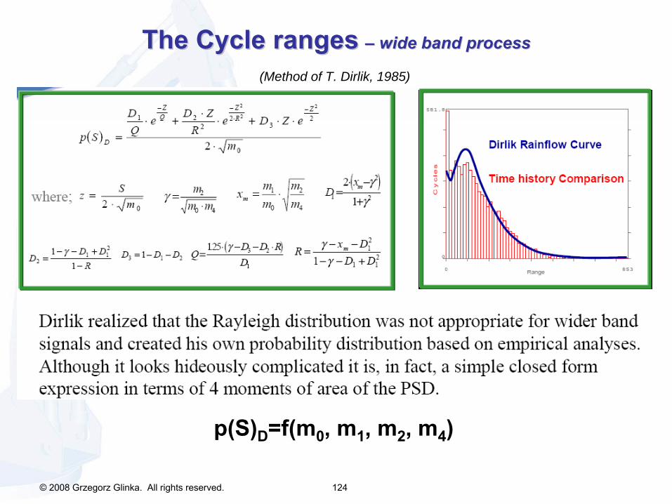
© 2008 Grzegorz Glinka. All rights reserved. 124
The The Cycle rangesCycle ranges
––
widewide
band band processprocess
(Method of T. Dirlik, 1985)
p(S)D
=f(m0
, m1
, m2
, m4
)