UvA-DARE is a service provided by the library of the University of Amsterdam (http://dare.uva.nl)

UvA-DARE (Digital Academic Repository)

Micromechanics of nonlinear plastic modes

Lerner, E.

Published in:Physical Review E

DOI:10.1103/PhysRevE.93.053004

Link to publication

Citation for published version (APA):Lerner, E. (2016). Micromechanics of nonlinear plastic modes. Physical Review E, 93(5), [053004].https://doi.org/10.1103/PhysRevE.93.053004

General rightsIt is not permitted to download or to forward/distribute the text or part of it without the consent of the author(s) and/or copyright holder(s),other than for strictly personal, individual use, unless the work is under an open content license (like Creative Commons).

Disclaimer/Complaints regulationsIf you believe that digital publication of certain material infringes any of your rights or (privacy) interests, please let the Library know, statingyour reasons. In case of a legitimate complaint, the Library will make the material inaccessible and/or remove it from the website. Please Askthe Library: https://uba.uva.nl/en/contact, or a letter to: Library of the University of Amsterdam, Secretariat, Singel 425, 1012 WP Amsterdam,The Netherlands. You will be contacted as soon as possible.

Download date: 16 Jun 2020

PHYSICAL REVIEW E 93, 053004 (2016)

Micromechanics of nonlinear plastic modes

Edan LernerInstitute for Theoretical Physics, Institute of Physics, University of Amsterdam, Science Park 904, 1098 XH Amsterdam, the Netherlands

(Received 17 March 2016; published 16 May 2016)

Nonlinear plastic modes (NPMs) are collective displacements that are indicative of imminent plastic instabilitiesin elastic solids. In this work we formulate the atomistic theory that describes the reversible evolution of NPMs andtheir associated stiffnesses under external deformations. The deformation dynamics of NPMs is compared to thoseof the analogous observables derived from atomistic linear elastic theory, namely, destabilizing eigenmodes ofthe dynamical matrix and their associated eigenvalues. The key result we present and explain is that the dynamicsof NPMs and of destabilizing eigenmodes under external deformations follow different scaling laws with respectto the proximity to imminent instabilities. In particular, destabilizing modes vary with a singular rate, whereasNPMs exhibit no such singularity. As a result, NPMs converge much earlier than destabilizing eigenmodes totheir common final form at plastic instabilities. This dynamical difference between NPMs and linear destabilizingeigenmodes underlines the usefulness of NPMs for predicting the locus and geometry of plastic instabilities,compared to their linear-elastic counterparts.

DOI: 10.1103/PhysRevE.93.053004

I. INTRODUCTION

When a disordered elastic solid is subjected to externaldeformation, particle-scale plastic instabilities are inevitablyencountered [1], each accompanied by a rearrangement ofa small set of particles conventionally coined as a “sheartransformation,” and some degree of energy dissipation [2–4].The occurrence rate, micromechanical consequences, andinteractions between these instabilities determine the macro-scopic rate of plastic deformation, which is a key rheologicalobservable that controls important material properties such astoughness and elastic limit [5].

The micromechanical process that takes place as plasticinstabilities are triggered under athermal conditions has beenthoroughly studied in the framework of atomistic linear elastic-ity [6–8]. In this framework, plastic instabilities that interruptreversible elastic branches [illustrated in, e.g., Fig. 1(b)] arereflected by the continuous vanishing of the lowest eigenvalueλp of the dynamical matrix M ≡ ∂2U

∂ �x∂ �x (see Appendix A fortensoric notation conventions) as the imposed shear strain γ

approaches an instability strain γc. Here and in what follows, �xdenotes the multidimensional coordinate vector of all particles’positions, and U (�x) denotes the potential energy. In thepotential energy landscape (PEL) picture, plastic instabilitiesare understood as the coalescence and mutual annihilationof a local minimum and a nearby first-order saddle point, aprocess known as a saddle-node bifurcation, at some criticalinstability strain γc. This implies that asymptotically close tothe instability strain, i.e., as γ → γc, the eigenvalue associatedwith the destabilizing eigenmode depends on the strain asλp ∼ √

γc − γ . In Fig. 1 key micro- and macroscopic aspectsof the mechanics of plastic instabilities are reviewed.

Plastic instabilities are cleanly captured by destabilizingeigenmodes only very close (in strain) to instability strains, andmore so as larger systems are considered, due to hybridizationprocesses of destabilizing eigenmodes with low-energy planewaves. This is not the case, however, with nonlinear plasticmodes (NPMs), introduced first in Ref. [9]. NPMs arecollective displacement directions which are indicative of thespatial structure and geometry of imminent plastic instabilities.

Their definition, which is solely based on inherent structureinformation, hinges on properly accounting for the relevantanharmonicities of the potential energy landscape, as shown inRef. [9] and explained in what follows. In this work we showthat NPMs closely resemble plastic instabilities well awayfrom instability strains and well before destabilizing modesdo. This is the case since NPMs do not “compete” with otherlow-frequency modes for their identity as the lowest-lyingnormal mode. They therefore do not suffer hybridizations withother modes, which leads to the preservation of their spatialstructure remarkably far (in strain) from plastic instabilities.This superior robustness of NPMs identities renders theirspatial distribution useful as means for a microstructuralcharacterization of disordered solids that controls plasticdeformation rates.

In this work we present a micromechanical theory forthe athermal quasistatic deformation-dynamics of NPMs(i.e., their evolution under imposed deformations) and theirassociated stiffnesses upon approaching plastic instabilities.The NPM’s deformation dynamics is compared to that of theconventional set of “linear” observables, namely, the destabi-lizing eigenmodes of the dynamical matrix and their associatedeigenvalues. In addition to demonstrating the persistence ofNPMs’ identities over very large strain scales away fromplastic instabilities, we further show that NPMs convergemuch faster scaling-wise to their form at the instability strains,compared to destabilizing eigenmodes. We present a scalinganalysis that explains the qualitative differences observedbetween the deformation dynamics of these two types ofmodes.

This manuscript is organized as follows: in Sec. II webriefly describe the numerical methods and models used inthis work. Further details about the numerics and algorithmsused are provided in Appendix B, and explanations of thetensor notations used throughout our work can be found inAppendix A. In Sec. III we review the conventional mi-cromechanical theory of plastic instabilities, discuss its rangeof applicability, and validate the theory against numericalsimulations. In Sec. IV we reintroduce the barrier function, putforward first in Ref. [9], from which the definition of NPMs

2470-0045/2016/93(5)/053004(12) 053004-1 ©2016 American Physical Society

EDAN LERNER PHYSICAL REVIEW E 93, 053004 (2016)

10−8

10−6

10−4

10−2

10−3

10−2

10−1

100

2

1

γc −γ

λp

loca

lized

extended

−4 −2 0 2 4 6 8

x 10−6

−5

0

5

10

15

20

25x 10

−19

s

δUΨ(s

)

γ → γc

0 γσ

γc

(a) (b)

(d)

(e) (f)

(c)

Ψp , γc − γ � 10−14 Ψp , γc − γ � 10−2

FIG. 1. Review of the micromechanics of a plastic instability. (a) An illustration of the basic setup considered in this work: an athermalglass under quasistatic simple shear deformation. (b) Cartoon of a typical stress σ vs strain γ signal in our setup; at some instability strain γc aplastic instability occurs. The dashed frame shows that close to the instability the stress follows σ − σc ∼ √

γc − γ , as shown, e.g., in Ref. [7].(c) Lowest eigenvalue λp = M : �p�p of the dynamical matrix M, vs the distance in strain γc − γ to the instability. Away from the instabilitythe eigenmode �p associated with λp is delocalized, as demonstrated in panel (f), and λp is largely insensitive to the deformation. As the solid isfurther deformed �p destabilizes and localizes, as demonstrated in panel (e). λp then vanishes as

√γc − γ . (d) Energy variations δU� (s) upon

displacing the particles about the mechanical equilibrium state according to δ�x = s�p , measured at distances γc − γ = 10−14, 10−41/3, 10−40/3,and 10−13 away from the instability strain. These curves demonstrate the well-understood saddle-node bifurcation which characterizes plasticinstabilities, in which a saddle point and minimum on the potential energy landscape coalesce and mutually annihilate, as shown in Refs. [6–8].The continuous lines are obtained by a cubic Taylor expansion of the energy variation, for which the expansion coefficients were calculatedusing inherent state information.

emerges. We present results from a numerical investigation ofthe spatial properties of NPMs, which are important for under-standing NPMs’ deformation dynamics. We further presentthe micromechanical theory that describes the deformationdynamics of stiffnesses associated with NPMs. In Sec. Vwe derive the micromechanical theory for the deformationdynamics of destabilizing modes and NPMs and presentdata from numerical simulations that validate the theory’spredictions. We end with a summary and discussion in Sec. VI.

II. METHODS AND MODELS

We provide here a brief overview of the numerics usedin our work; a complete and detailed description is providedin Appendix B. We employed a simple glass former in twodimensions that consists of pointlike particles interacting viainverse power-law purely repulsive pairwise potentials. Weexpect our results to be independent of this particular choiceof model. An example of a snapshot of our model glass

with N = 1600 is displayed in Fig. 1(a). We investigatedsystems of N = 402, 802, 1602, and 3202 particles; for eachsystem size, we selected a single realization for which thefirst plastic instability upon shearing occurred at a strainγc � 10−3. No other considerations were used when selectingeach realization for the subsequent analyses carried out. Alldeformation simulations were carried out under athermal, qua-sistatic conditions, and the imposed deformation was simpleshear under Lees-Edwards periodic boundary conditions. Here128-bit numerics were employed to enable approaching plasticinstabilities up to strains of the order of γc − γ ∼ 10−14. Thecalculation of nonlinear plastic modes (defined in Sec. IV) isexplained in Appendix B.

III. PLASTIC INSTABILITIES AS REFLECTED BYATOMISTIC LINEAR ELASTICITY

In this section we review the conventional atomistic theoryof plastic instabilities in disordered elastic solids. The majority

053004-2

MICROMECHANICS OF NONLINEAR PLASTIC MODES PHYSICAL REVIEW E 93, 053004 (2016)

of the formalism presented in this section appears in, e.g.,Refs. [7,8,10,11]; it is summarized here for the sake ofcompleteness.

We consider a disordered system of N particles in đdimensions, enclosed in a box of volume � under periodicboundary conditions, and interacting via some potential energyU (�x) which is a function of the particles’ coordinates �x.Here and in all that follows, we restrict the discussion to theathermal limit T → 0, with T denoting the temperature. Inthe athermal limit, as long as it is mechanically stable, thesystem resides in a local minimum of the potential energy,i.e., in a state �x0 of mechanical equilibrium. This means that(1) ∂U

∂ �x |�x0= 0 and (2) all eigenvalues of the dynamical matrix

M ≡ ∂2U∂ �x∂ �x |�x0

are non-negative (see Appendix A for tensoricnotation conventions).

We next consider what happens when we deform our solidunder quasistatic shear deformation, and in particular, we studyhow the eigenvalues of M vary as deformation is imposed. Westart by writing the eigenmode decomposition of the dynamicalmatrix as

M =Nd−∑=0

�, (1)

where the orthonormal eigenmodes � satisfy the eigenvalueequation

M · � = λ�, (2)

and therefore λ = M : ��. We aim to spell out thedeformation dynamics of the eigenvalues, namely, to derivean equation for dλ

dγ. In the athermal limit, total derivatives

with respect to strain are taken according to [7,8,12,13]

d

dγ= ∂

∂γ+ d �x

dγ· ∂

∂ �x , (3)

where d �xdγ

denotes what are known as the nonaffine part ofthe deformation dynamics of the particles’ coordinates. Anexplicit expression for d �x

dγcan be derived by requiring that

mechanical equilibrium is preserved under the deformation,namely,

d

dγ

∂U

∂ �x = ∂2U

∂γ ∂ �x + d �xdγ

· ∂2U

∂ �x∂ �x = 0, (4)

which can be inverted in favor of d �xdγ

, as

d �xdγ

= −M−1 · ∂2U

∂ �x∂γ. (5)

The superscript −1 should be understood here and in whatfollows as denoting the inverse of an operator taken afterremoving its zero modes. This removal is justified by theperfect orthogonality of the contracted vector with the zeromodes of the inverted operator (which will always be thecase in what follows). Equations (3) and (5), introduced firstin Ref. [12], are central for the calculations presented in thesubsequent sections.

Using the formalism explained above, we take the derivativeof an eigenvalue of M as

dλ

dγ= dM

dγ:�� = ∂M

∂γ:�� + U ′′′ .

:��

d �xdγ

, (6)

where U ′′′ ≡ ∂3U∂ �x∂ �x∂ �x , and no additional terms appear since

normalization of modes implies that d�

dγ·� = 0. Using the

eigenmode decomposition of the dynamical matrix in Eq. (5),and inserting it in Eq. (6) we find

dλ

dγ= ∂M

∂γ:�� −

∑m

(U ′′′ .:���m)

(�m · ∂2U

∂ �x∂γ

)λm

. (7)

Equation (7) describes the deformation dynamics of anyof the Nd− eigenvalues λ of M. Here we focus in particularon the equation for the lowest eigenvalue λp; as a plasticinstability at a strain γc is approached λp → 0, and the RHSin the above equation is then dominated by the term in thesum pertaining to the destabilizing mode [an example of thelatter can be seen in Fig. 1(e)]. As γ → γc, we can thereforeapproximate

dλp

dγ

∣∣∣∣γ→γ −

c

� −τpνp

λp

, (8)

where we have defined the asymmetry of a mode � as τ ≡U ′′′ .

: ���, and its shear-force coupling as ν ≡ ∂2U∂γ ∂ �x · �.

This limiting differential equation, together with the boundarycondition λp(γc) = 0, can be trivially solved for λp as

λp(γ → γ −c ) � √

2τpνp

√γc − γ , (9)

where we have assumed that τp and νp are regular at γc. InFig. 1(c) the scaling λp ∼ √

γc − γ is confirmed by computersimulations.

Let us review two important consequences of Eq. (9),demonstrated in Fig. 1. First, on the macroscopic level, theshear stress and modulus also show signatures of plasticinstabilities, which are derivable from Eq. (9); in the athermallimit, the shear modulus is given by [7,8,12]

μ = 1

�

(∂2U

∂γ 2+ ∂2U

∂γ ∂ �x · d �xdγ

). (10)

As γ → γc, λp → 0, then d �xdγ

= −∑

ν

λ� → − νp

λp�p, and

the shear modulus can be approximated as

μ � − ν2p

λp

∼ −(γc − γ )−12 . (11)

Consequently, the departure of the stress from its value σc atthe instability strain is expected to follow

σ − σc ∼ √γc − γ , (12)

as illustrated in the cartoon in Fig. 1(b), and shown in, e.g.,Ref. [7].

Equation (9) also leads to insights on the microscopicmechanics; we define δU�(s) as the variation of the potentialenergy upon displacing the particles about the inherent state�x0 according to δ�x ≡ �x − �x0 = s�p. For small distances s we

053004-3

EDAN LERNER PHYSICAL REVIEW E 93, 053004 (2016)

can expand δU�(s) as

δU�(s) � 12λps2 + 1

6τps3. (13)

Figure 1(d) displays the energy variations δU�(s) obtainedat various strains approaching a plastic instability strain γc.The softening of the stiffness λp = d2U

ds2 upon approachingthe instability, as predicted by Eq. (9), is apparent, as is thedecreasing of the saddle point. From Eq. (13) we deduce thatthe saddle point occurs at s� = −2 λp

τp, with a magnitude of

δU�(s�) = 23

λ3p

τ 2p

∼ (γc − γ )32 following Eq. (9), as shown in

Refs. [10,11].How far away from the instability strain γc is Eq. (9) valid?

This depends on the strain scale in which the dehybridizationof the destabilizing mode from the lowest plane waves occurs,which can be estimated by comparing the stiffness associatedwith the lowest energy shear wave in a system of linear sizeL, to the stiffness of the destabilizing mode λp. The formeris expected to scale as L−2, while the latter is proportional to√

τpνp

√γc − γ . Equation (9) is therefore expected to hold at

up to strain intervals γc − γ � 1/(τpνpL4), as indeed shownto hold numerically in Fig. 2. In what follows we will showthat this strain scale is central to the deformation dynamics ofdestabilizing modes.

10−10

10−8

10−6

10−4

10−2

10−5

10−4

10−3

10−2

10−1

100

γc −γ

λp

10−2

100

102

104

106

108

1010

10−1

100

101

102

103

2

1

(γc −γ)τpνpL4

λpL

2

N = 402

N = 802

N = 1602

N = 3202

(a)

(b)

FIG. 2. (a) The eigenvalues λp associated with destabilizingmodes �p vs distance in strain γc − γ to a plastic instability strainγc, for various system sizes as shown in the legend. The instabilitieswere the first encountered upon shearing a randomly selected freshlyquenched glass. (b) Rescaled λp vs the rescaled strain interval revealsthat Eq. (9) holds on intervals below the scale δγ ∼ 1/(τpνpL4).

τp ≡ U ′′′ .: �p�p�p and νp ≡ ∂2U

∂γ ∂ �x · �p were calculated at γc − γ �10−13.

IV. NONLINEAR PLASTIC MODES (NPMS)

A. Introduction and definitions

The strain scale 1/(τpνpL4), below which plastic insta-bilities are robustly reflected by the destabilizing mode,quickly vanishes for large systems. An important questionis therefore whether modes that are indicative of imminentplastic instabilities can be defined and detected away frominstability strains, at scales γc − γ 1/(τpνpL4). In otherwords, is it possible to overcome the difficulties associatedwith the hybridization of destabilizing modes with planewaves in the detection of imminent plastic instabilities? InRef. [9] this question was answered to the affirmative: itwas shown that nonlinear plastic modes (NPMs) exhibitremarkable resemblance to dehybridized destabilizing modesand can be detected well before plastic instabilities, deep inthe regime where the destabilizing mode is fully hybridizedwith plane waves.

The theoretical framework within which the definition ofNPMs emerges is constructed as follows: consider the variationδUz(s) of the potential energy upon displacing the particlesabout the inherent state �x0, but this time along a generalcollective displacement direction (mode) z (which may or maynot be an eigenmode of M), namely, according to δ�x = sz.For small s, it writes

δUz(s) � 12κzs

2 + 16τzs

3, (14)

where we have introduced the stiffness κz ≡ M : zz andthe asymmetry τz ≡ U ′′′ .

: zzz associated with the collectivedisplacement direction z. Notice that the first order term inEq. (14) is absent due to mechanical equilibrium, and z isdimensionless and normalized, i.e., z · z = 1. In its truncatedform Eq. (14), δUz possesses stationary points at s = 0 ands� = − 2κz

τz, corresponding respectively to a minimum and

maximum of the truncated potential energy variation along thereaction coordinate s. We emphasize that Eq. (14) differs fromEq. (13) by describing the energy variation upon displacingthe particles along a general direction z in the former case, asopposed to along the eigenmode �p in the latter.

We next define the truncated energy variation at themaximum s� as the “barrier function” b(z), namely,

b(z) ≡ 1

2κzs

2� + 1

6τzs

3� = 2κ3

z

3τ 2z

. (15)

Notice that b(z) is not a function of the reaction coordinates, but instead a function of the multidimensional collectivedisplacement direction z. By construction, modes z for whichb(z) is small are characterized by small stiffnesses κz and largeasymmetries τz. This, in turn, implies that the displacementdistance s� for those modes is small, and therefore thecubic expansion at distances s ∼ s� should be a faithfulrepresentation of the actual variation of the potential energyupon displacing the particles along z, as demonstrated, e.g., fordestabilizing modes in Fig. 1(d). Thus, small enough b shouldpertain to actual saddle points (energy barriers) that separatebetween the inherent structure in which the system resides andneighboring ones.

NPMs are therefore defined as modes π for which b attains alocal minimum. This means that modes π satisfy ∂b

∂�z |�z=π = 0,

053004-4

MICROMECHANICS OF NONLINEAR PLASTIC MODES PHYSICAL REVIEW E 93, 053004 (2016)

and all eigenvalues of the linear operator ∂2b∂�z∂�z |�z=π are non-

negative. Local minima of b do not guarantee the smallnessof b and therefore do not necessarily faithfully indicate anactual instability direction. Nevertheless, modes π that pertainto low-lying minima of b are indicative of directions that takethe system over saddle points of the potential energy and inparticular indicate imminent plastic instabilities, as shown inRef. [9].

At this point it is useful to note that the barrier functionis invariant to variations of the norm of its vector argument,i.e., b(z) = b(cz) for any finite c. This means that the barrierfunction can be equivalently expressed as a function of a setof Nd− independent variables �z, as

b(�z) = 2

3

(M : �z�z)3

(U ′′′ .: �z�z�z)2

. (16)

In turn, this allows us to meaningfully take partial derivativeswith respect to those variables, and in particular

∂b

∂�z = 4κ2

�zτ 2�z

(M · �z − κ�z

τ�zU ′′′ : �z�z

). (17)

The gradient ∂b∂�z with respect to �z given above vanishes when

evaluated at NPMs π , the latter are therefore solutions to thenonlinear equation

M · π = κπ

τπ

U ′′′ : π π . (18)

Equation (18) is key to the deformation dynamics of NPMsand has an interesting geometric interpretation; to see this,imagine we displace the constituent particles about the inherentstructure configuration according to δ�x = sπ . The quadraticexpansion in s of the force response that results from thisdisplacement is

�Fπ (s) � −M · π s − 12U ′′′ : π π s2. (19)

Equation (18) says that the linear and nonlinear coefficientsof the force response expansion are parallel Nd− dimensionalvectors.

What is the spatial structure of the said force response,and in particular of the parallel vectors M · π and U ′′′ : π π?In Ref. [9] it was shown that NPM’s structure consists of adisordered, localized core, decorated by long-range largelyaffine displacement fields that decay away from the core as|π |(r) ∼ r1−d− , where r denotes the distance from the NPM’score center. The force response �Fπ is given by a doublecontraction of π with the third order tensor U ′′′; we thereforeexpect the relative magnitude of the force response away fromthe NPM’s core to scale as the gradient squared of π , namely,

| �Fπ |(r) ∼ |∇π |2(r) ∼ r−2d− . (20)

This relation is further motivated in Appendix C, for the simplecase of pairwise central-force potentials.

To verify Eq. (20) numerically, we define the spatial decayprofiles C�v(r), which are calculated on a vector �v by taking themedian over the square of all components of the normalizedv that are situated at a distance ≈ r away from the coreof a plastic instability; see Ref. [9] for further details. InFig. 3(a) we plot the decay profiles of a NPM π (calculatedas explained in Appendix B) and a destabilizing mode �p

100

101

102

10−4

10−3

10−2

10−1

100

1

2

r

C(r)

πΨp ∝ M· Ψp

δR

100

101

102

10−15

10−10

10−5

100

1

8

r

C(r)

U : ππ ∝ M· πU : ΨpΨp

U : δRδR

(b)

(a)

FIG. 3. (a) Spatial decay profiles C(r) (see text for definition)of a NPM π and of a destabilizing eigenmode �p calculated in asystem of N = 102 400 at a distance γc − γ ∼ 10−14 away from aplastic instability. Also plotted is the decay profile of the responseδ �R = M−1 �d to a local dipolar force �d . All these modes are foundto decay as r−1 (notice that C scales as the magnitude squared of amode’s components). (b) The nonlinear force responses of the samemodes analyzed in panel (a) decay as r−4. We verify that the doublecontraction of a spatially decaying mode with U ′′′, e.g., U ′′′ : �p�p ,picks up the square of the spatial gradient of that mode, in consistencywith Eq. (20). Notice that the linear and nonlinear force responses ofthe NPM π are parallel, therefore |M · π |(r) ∼ r−4 as well, while|M · �|(r) ∼ r−1.

measured close to a plastic instability. These decay profilesare compared to that calculated for the displacement responseδ �R = M−1 �d to a local dipolar force �d (as described in,e.g., Ref. [14]) in an undeformed solid. All three modes arefound to decay as r−1 (in our two-dimensional simulations).In Fig. 3(b) we plot the spatial decay profiles of the doublecontractions of these three modes with the third-order tensorU ′′′. We indeed find that Cπ ∼ r−2 and CM·π ∼ CU ′′′:π π ∼ r−8

implying that |π |(r) ∼ r−1, and |M·π |(r) ∼ |U ′′′ : π π |(r) ∼r−4, supporting Eq. (20).

The above discussion and the data plotted in Fig. 3 lead toan interesting conclusion: although destabilizing modes andNPMs share the same spatial decay profiles, the linear forceresponses M−1 · �p and M−1 · π do not; the former decayaway from the disordered core as r1−d− (just as the destabilizingmodes themselves), whereas the latter decay as r−2d− .

053004-5

EDAN LERNER PHYSICAL REVIEW E 93, 053004 (2016)

B. Dynamics of NPM stiffnesses

We next show that the deformation dynamics of NPMsstiffnesses κπ = M : π π and of the eigenvalues λp = M :�p�p obey the same equation of motion close to plasticinstabilities. The total derivative with respect to deformationof the stiffness reads

dκπ

dγ= dM

dγ: π π + 2M :

dπ

dγπ

= U ′′′ .: π π

d �xdγ

+ ∂M∂γ

: π π + 2M :dπ

dγπ .

Notice next that the first term on the RHS of the above equationcan be written using Eqs. (5) and (18) as

U ′′′ .: π π

d �xdγ

= − τπ

κπ

π · M · M−1 · ∂2U

∂ �x∂γ= −τπ νπ

κπ

, (21)

and therefore we arrive at

dκπ

dγ= −τπ νπ

κπ

+ ∂M∂γ

: π π + 2M :dπ

dγπ . (22)

The vanishing of κπ upon plastic instabilities also impliesthat |M · π | → 0. Assuming that | dπ

dγ| � |M · π |−1 as plastic

instabilities are approached (an assumption that will beestablished in the following section), and recalling that ∂M

∂γis

always regular, the last two terms in the right-hand side of theabove equation can be neglected close to plastic instabilities,and we are left with

dκπ

dγ

∣∣∣∣γ→γ −

c

� −τπ νπ

κπ

. (23)

This limiting differential equation is identical in structure toEq. (9) for the deformation dynamics of the eigenvalues λp

associated with destabilizing eigenmodes �p. It is thereforesolved by

κπ (γ → γ −c ) �

√2τπ νπ

√γc − γ , (24)

which is verified numerically in Fig. 4.One important observation to note is that Eq. (24) is

followed over large strain intervals γc − γ , without a clearsystem-size dependence, as can be seen in Fig. 4. This standsin contrast with what is seen for the eigenvalues of destabilizingmodes as described by Eq. (9), which is valid only overscales γc − γ � L−4. This difference arises since NPMs do not“compete” for their identity with other low-frequency normalmodes, i.e., they do not suffer hybridizations.

One obvious limitation on the range over which Eq. (24)is valid is the extent of typical elastic branches betweenconsecutive plastic instabilities, which has been shown tovanish as N−β with β ≈ 2/3 [1,15]. We therefore assert thatabove some system size the deformation dynamics of NPMsassociated with imminent plastic instabilities will always bedescribed by Eq. (24).

Finally, we underline an important consequence of thesimultaneous vanishing of the eigenmode λp and the stiffnessκ at the same instability strain: both the destabilizing mode� and the NPM π must converge to a common final format the instability strain, since at that point they both satisfyM · �p = M · π = 0 and must therefore be equal. This

10−10

10−8

10−6

10−4

10−2

10−5

10−3

10−1

101

2

1

γc −γ

κπ

10−10

10−8

10−6

10−4

10−2

0.8

1

1.2

1.4

1.6

γc −γ

κπ

√2τ

πν

π√

γc−

γ

N = 402

N = 802

N = 1602

N = 3202

(a)

(b)

FIG. 4. (a) Stiffnesses κπ vs strain interval γc − γ . The palesymbols represent the eigenvalues λp , which perfectly coincide withthe κπ as γ → γc. (b) Rescaling the stiffnesses by their asymptoticform κπ � √

2τπ νπ

√γc − γ verifies Eq. (24) and shows that this

scaling breaks down at a strain scale with no clear system-sizedependence, in stark contrast with the eigenvalues λp shown in Fig. 2.Nevertheless, up to strain intervals γc − γ � 10−3, we find that thedeviations from the asymptotic form remain less than roughly 50%.

convergence of the two modes at a plastic instability isvalidated in Fig. 5.

V. DEFORMATION DYNAMICS OF LINEAR ANDNONLINEAR MODES

We have seen theoretically and numerically that the stiff-nesses associated with destabilizing modes and NPMs are en-slaved to the same equation of motion at scales γc − γ � L−4

away from plastic instabilities. Is there a similar equivalencebetween the deformation dynamics of the destabilizing modeand that of the NPM? In this section we derive exact equationsof motion for the NPM and destabilizing mode associated witha plastic instability. A scaling analysis close to the instabilityreveals the surprising finding that the deformation dynamicsof these two mode types follow different scaling laws, bothwith respect to the distance to the instability strain and withrespect to system size. In particular, we find that

∣∣∣∣d�p

dγ

∣∣∣∣2

∼ L4

γc − γand

∣∣∣∣dπ

dγ

∣∣∣∣2

∼ const, (25)

as shown numerically in Figs. 6 and 7.

053004-6

MICROMECHANICS OF NONLINEAR PLASTIC MODES PHYSICAL REVIEW E 93, 053004 (2016)

10−10

10−8

10−6

10−4

10−2

10−8

10−6

10−4

10−2

100

γc −γ

1−

π·Ψ

p

10−2

100

102

104

106

108

10−8

10−6

10−4

10−2

100

1

1

(γc −γ)τpνpL4

1−

π·Ψ

p

N = 402

N = 802

N = 1602

N = 3202

(a)

(b)

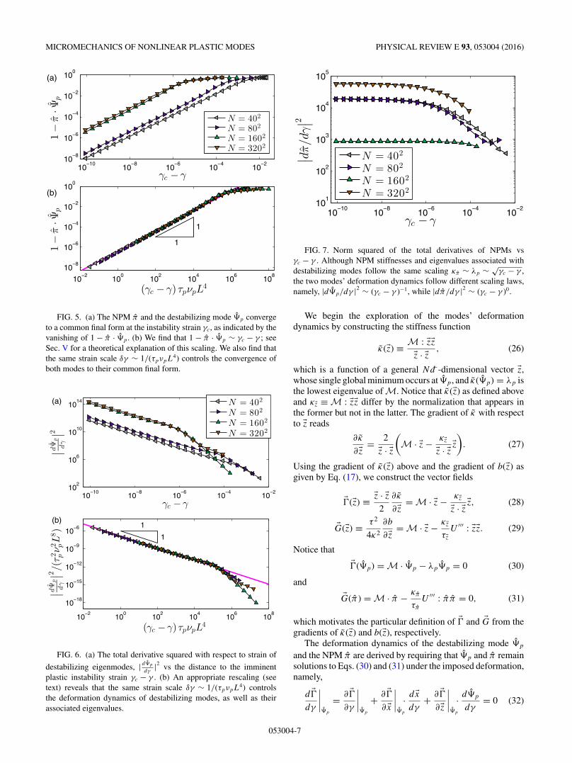
FIG. 5. (a) The NPM π and the destabilizing mode �p convergeto a common final form at the instability strain γc, as indicated by thevanishing of 1 − π · �p . (b) We find that 1 − π · �p ∼ γc − γ ; seeSec. V for a theoretical explanation of this scaling. We also find thatthe same strain scale δγ ∼ 1/(τpνpL4) controls the convergence ofboth modes to their common final form.

10−10

10−8

10−6

10−4

10−2

102

106

1010

1014

γc −γ

dΨ

p

dγ

2

10−2

100

102

104

106

108

10−18

10−15

10−12

10−9

10−6 1

1

(γc −γ)τpνpL4

dΨ

p

dγ

2 /(τ

2 pν

2 pL

8 )

N = 402

N = 802

N = 1602

N = 3202

(a)

(b)

FIG. 6. (a) The total derivative squared with respect to strain of

destabilizing eigenmodes, | d�p

dγ|2 vs the distance to the imminent

plastic instability strain γc − γ . (b) An appropriate rescaling (seetext) reveals that the same strain scale δγ ∼ 1/(τpνpL4) controlsthe deformation dynamics of destabilizing modes, as well as theirassociated eigenvalues.

10−10

10−8

10−6

10−4

10−2

101

102

103

104

105

γc −γ

dπ/d

γ2

N = 402

N = 802

N = 1602

N = 3202

FIG. 7. Norm squared of the total derivatives of NPMs vsγc − γ . Although NPM stiffnesses and eigenvalues associated withdestabilizing modes follow the same scaling κπ ∼ λp ∼ √

γc − γ ,the two modes’ deformation dynamics follow different scaling laws,namely, |d�p/dγ |2 ∼ (γc − γ )−1, while |dπ/dγ |2 ∼ (γc − γ )0.

We begin the exploration of the modes’ deformationdynamics by constructing the stiffness function

κ(�z) ≡ M : �z�z�z · �z , (26)

which is a function of a general Nd−-dimensional vector �z,whose single global minimum occurs at �p, and κ(�p) = λp isthe lowest eigenvalue of M. Notice that κ(�z) as defined aboveand κ�z ≡ M : �z�z differ by the normalization that appears inthe former but not in the latter. The gradient of κ with respectto �z reads

∂κ

∂�z = 2

�z · �z(M · �z − κ�z

�z · �z �z)

. (27)

Using the gradient of κ(�z) above and the gradient of b(�z) asgiven by Eq. (17), we construct the vector fields

��(�z) ≡ �z · �z2

∂κ

∂�z = M · �z − κ�z�z · �z �z, (28)

�G(�z) ≡ τ 2

4κ2

∂b

∂�z = M · �z − κ�zτ�z

U ′′′ : �z�z. (29)

Notice that

��(�p) = M · �p − λp�p = 0 (30)

and

�G(π ) = M · π − κπ

τπ

U ′′′ : π π = 0, (31)

which motivates the particular definition of �� and �G from thegradients of κ(�z) and b(�z), respectively.

The deformation dynamics of the destabilizing mode �p

and the NPM π are derived by requiring that �p and π remainsolutions to Eqs. (30) and (31) under the imposed deformation,namely,

d ��dγ

∣∣∣∣�p

= ∂ ��∂γ

∣∣∣∣�p

+ ∂ ��∂ �x

∣∣∣∣�p

· d �xdγ

+ ∂ ��∂�z

∣∣∣∣�p

· d�p

dγ= 0 (32)

053004-7

EDAN LERNER PHYSICAL REVIEW E 93, 053004 (2016)

and

d �Gdγ

∣∣∣∣π

= ∂ �G∂γ

∣∣∣∣π

+ ∂ �G∂ �x

∣∣∣∣π

· d �xdγ

+ ∂ �G∂�z

∣∣∣∣π

· dπ

dγ= 0. (33)

Equations (32) and (33) can be inverted in favor of d�p

dγand

dπdγ

as

d�p

dγ= −

(∂ ��∂�z

)∣∣∣∣−1

�p

·(

∂ ��∂γ

∣∣∣∣�p

+ ∂ ��∂ �x

∣∣∣∣�p

· d �xdγ

)(34)

and

dπ

dγ= −

(∂ �G∂�z

)∣∣∣∣−1

π

·(

∂ �G∂γ

∣∣∣∣π

+ ∂ �G∂ �x

∣∣∣∣π

· d �xdγ

). (35)

The analysis of the scaling properties of Eqs. (34) and (35)with respect to γc − γ starts with realizing that �p and π

are zero modes of ∂ ��∂�z |�p

and ∂ �G∂�z |π , respectively, and therefore

( ∂ ��∂�z )|−1

�pand ( ∂ �G

∂�z )|−1π (defined as taken after removal of the

zero modes) are regular as γ → γc. Furthermore, the vectors∂ ��∂γ

and ∂ �G∂γ

are expected to converge to regular values at plasticinstabilities as well. We conclude thus that any singularity

that d�p

dγand dπ

dγmight possess can be inherited only from the

singularity of d �xdγ

[recall that | d �xdγ

| ∼ (γc − γ )−1/2].

A. Deformation dynamics of destabilizing modes

Let us focus first on d�p

dγas given by Eq. (34); close to

instabilities we can approximate d �xdγ

� − νp

λp�p, then

d�p

dγ� νp

λp

(M − λpI)−1 · (U ′′′ : �p�p − τp�p), (36)

which is singular in terms of γc − γ following the scaling ofλp ∼ √

γc − γ .In Fig. 3 it was shown that � decays at distances r away

from its core as r1−d− , and U ′′′ : �p�p decays as r−2d− , the for-mer therefore dominates the difference U ′′′ : �p�p − τp�p

as appears in Eq. (36), at large r . This difference thereforecouples strongly to the lowest-lying eigenmodes of M − λpIin Eq. (36), which are plane waves with frequencies of orderL−1. This is further corroborated in Fig. 8, where we plot the

field d�p

dγwhich displays the same geometry as displayed by the

lowest-frequency plane waves of the system. We thus expect∣∣∣∣d�p

dγ

∣∣∣∣2

∼ τ 2pν2

pL4

λ2p

∼ τpνpL4

γc − γ, (37)

as found in our numerical simulations; see Fig. 6.

B. Deformation dynamics of NPMs

We finally turn to analyzing the scaling properties of the

equation of motion (35) for dπdγ

. As shown for the case of d�p

dγ,

the only way dπdγ

could be singular in γc − γ is if the right-hand

side of Eq. (35) inherits the singularity of d �xdγ

, whose norm

scales as (γc − γ )−1/2. It turns out, however, that ∂ �G∂ �x |π · d �x

dγis

FIG. 8. The field d�p

dγcalculated at γc − γ ∼ 10−14 away from a

plastic instability in a system of N = 6400 particles.

regular at γc; to see this, we first approximate this contractionclose to instabilities as

∂ �G∂ �x

∣∣∣∣π

· d �xdγ

� νp

λp

(U ′′′ .

: π π�p

τπ

U ′′′ : π π − U ′′′ : π�p

+ κz

τπ

U ′′′′ .: π π�p − κπU ′′′′ :

: π π π�p

τ 2π

U ′′′ : π π

), (38)

where U ′′′′ ≡ ∂4U∂ �x∂ �x∂ �x∂ �x is the fourth order tensor of derivatives

of the potential energy. It is clear that the last two terms on theright-hand side of the above equation are not singular (they areproportional to κz/λp, which approaches unity at the instabilitystrain). We therefore focus for a moment on the first two termson the right-hand side of Eq. (38); notice that

U ′′′ .: π π�p

τπ

U ′′′ : π π − U ′′′ : π�p

= U ′′′ .: π π ��τπ

U ′′′ : π π − U ′′′ : π ��, (39)

where we have defined the vector difference �� ≡ π − �p

between π and �p, and recall that τπ ≡ U ′′′ .: π π π . As the

instability strain is approached � ≡ | ��| → 0, then we canexpress �� as the solution to either one of the linear equations:

∂2κ

∂�z∂�z∣∣∣∣�p

· �� = ∂κ

∂�z∣∣∣∣π

, (40)

∂2b

∂�z∂�z∣∣∣∣π

· �� = −∂b

∂�z∣∣∣∣�p

. (41)

The two above equations are nothing more than the linearexpansion of the respective gradients of κ and b about theirminima at �p and π , respectively.

We focus on Eq. (40) since it is simpler in structure; takingthe partial derivatives, inverting in favor of ��, and using

053004-8

MICROMECHANICS OF NONLINEAR PLASTIC MODES PHYSICAL REVIEW E 93, 053004 (2016)

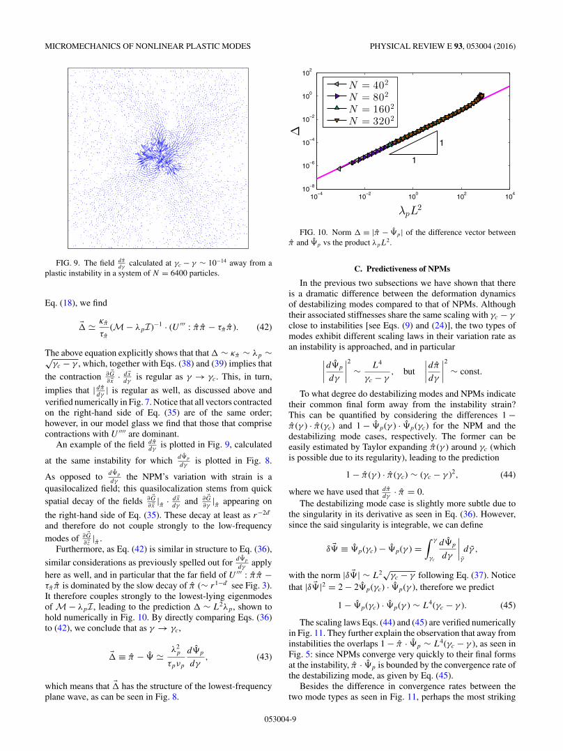
FIG. 9. The field dπ

dγcalculated at γc − γ ∼ 10−14 away from a

plastic instability in a system of N = 6400 particles.

Eq. (18), we find

�� � κπ

τπ

(M − λpI)−1 · (U ′′′ : π π − τπ π ). (42)

The above equation explicitly shows that that � ∼ κπ ∼ λp ∼√γc − γ , which, together with Eqs. (38) and (39) implies that

the contraction ∂ �G∂ �x · d �x

dγis regular as γ → γc. This, in turn,

implies that | dπdγ

| is regular as well, as discussed above andverified numerically in Fig. 7. Notice that all vectors contractedon the right-hand side of Eq. (35) are of the same order;however, in our model glass we find that those that comprisecontractions with U ′′′′ are dominant.

An example of the field dπdγ

is plotted in Fig. 9, calculated

at the same instability for which d�p

dγis plotted in Fig. 8.

As opposed to d�p

dγthe NPM’s variation with strain is a

quasilocalized field; this quasilocalization stems from quickspatial decay of the fields ∂ �G

∂ �x |π · d �xdγ

and ∂ �G∂γ

|π appearing on

the right-hand side of Eq. (35). These decay at least as r−2d−

and therefore do not couple strongly to the low-frequencymodes of ∂ �G

∂�z |π .Furthermore, as Eq. (42) is similar in structure to Eq. (36),

similar considerations as previously spelled out for d�p

dγapply

here as well, and in particular that the far field of U ′′′ : π π −τπ π is dominated by the slow decay of π (∼ r1−d− see Fig. 3).It therefore couples strongly to the lowest-lying eigenmodesof M − λpI, leading to the prediction � ∼ L2λp, shown tohold numerically in Fig. 10. By directly comparing Eqs. (36)to (42), we conclude that as γ → γc,

�� ≡ π − � � λ2p

τpνp

d�p

dγ, (43)

which means that �� has the structure of the lowest-frequencyplane wave, as can be seen in Fig. 8.

10−4

10−2

100

102

104

10−8

10−6

10−4

10−2

100

102

1

1

λpL2

Δ

N = 402

N = 802

N = 1602

N = 3202

FIG. 10. Norm � ≡ |π − �p| of the difference vector betweenπ and �p vs the product λpL2.

C. Predictiveness of NPMs

In the previous two subsections we have shown that thereis a dramatic difference between the deformation dynamicsof destabilizing modes compared to that of NPMs. Althoughtheir associated stiffnesses share the same scaling with γc − γ

close to instabilities [see Eqs. (9) and (24)], the two types ofmodes exhibit different scaling laws in their variation rate asan instability is approached, and in particular

∣∣∣∣d�p

dγ

∣∣∣∣2

∼ L4

γc − γ, but

∣∣∣∣dπ

dγ

∣∣∣∣2

∼ const.

To what degree do destabilizing modes and NPMs indicatetheir common final form away from the instability strain?This can be quantified by considering the differences 1 −π (γ ) · π (γc) and 1 − �p(γ ) · �p(γc) for the NPM and thedestabilizing mode cases, respectively. The former can beeasily estimated by Taylor expanding π (γ ) around γc (whichis possible due to its regularity), leading to the prediction

1 − π (γ ) · π(γc) ∼ (γc − γ )2, (44)

where we have used that dπdγ

· π = 0.The destabilizing mode case is slightly more subtle due to

the singularity in its derivative as seen in Eq. (36). However,since the said singularity is integrable, we can define

δ �� ≡ �p(γc) − �p(γ ) =∫ γ

γc

d�p

dγ

∣∣∣∣γ

dγ ,

with the norm |δ ��| ∼ L2√γc − γ following Eq. (37). Noticethat |δ ��|2 = 2 − 2�p(γc) · �p(γ ), therefore we predict

1 − �p(γc) · �p(γ ) ∼ L4(γc − γ ). (45)

The scaling laws Eqs. (44) and (45) are verified numericallyin Fig. 11. They further explain the observation that away frominstabilities the overlaps 1 − π · �p ∼ L4(γc − γ ), as seen inFig. 5: since NPMs converge very quickly to their final formsat the instability, π · �p is bounded by the convergence rate ofthe destabilizing mode, as given by Eq. (45).

Besides the difference in convergence rates between thetwo mode types as seen in Fig. 11, perhaps the most striking

053004-9

EDAN LERNER PHYSICAL REVIEW E 93, 053004 (2016)

10−10

10−8

10−6

10−4

10−2

10−15

10−10

10−5

100

1

1

1

2

γc − γ

1−

π(γ

)·π(γ

c),

1−

Ψp(γ

)·Ψ

p(γ

c)

N = 402

N = 802

N = 1602

N = 3202

FIG. 11. 1 − π(γ ) · π(γc) (outlined symbols) and 1 − �p(γ ) ·�p(γc) (solid symbols) vs γc − γ . NPMs converge must fasterscaling-wise to their final form at instabilities compared to desta-bilizing modes and are therefore better predictors of imminent plasticinstabilities.

feature of this data is the typical value measured for π(γ ) ·π (γc) when the NPMs are first detected, at strain scales onthe order of 10−3 away from the instability. At these strainsthe overlaps with the final form of the NPMs agree up to afew tenths of a percent, indicating that once detected, NPMsare nearly perfect indicators of the locus and geometry ofimminent plastic instabilities.

VI. SUMMARY AND OUTLOOK

We have carried out a comparative theoretical and nu-merical analysis of the deformation dynamics of nonlinearplastic modes and destabilizing eigenmodes upon approachingplastic instabilities. We have found that although the stiffnessesassociated with these two mode types follow the same scalingwith strain, the modes themselves vary with vastly differentrates as instabilities are approached. Not only do NPMs notsuffer from hybridizations with low-frequency normal modesas destabilizing modes do, but their variation rate is regularupon approaching plastic instabilities, in stark contrast withthe singular variation rate of destabilizing modes. These resultsadd substantial support to the usefulness of NPMs as robustplasticity predictors and to the role NPMs’ spatial distributionmay play as a state variable that controls the rate of plasticdeformation in glasses subjected to external loading.

The picture that emerges from our study is that the systemsize and strain dependence in the deformation dynamics ofdestabilizing mode stems from the dehybridization processthat continues to take place all the way up to the instabilitystrain. We find that close to plastic instabilities the destabilizingmode can be obtained by adding a plane-wave-like mode withan amplitude proportional to L2√γc − γ to the NPM. Thisinterpretation suggests that the most relevant objects to plastic

flow in disordered solids are NPMs, and that research effortsshould be focused on studying their statistics and dynamics.

Our analysis reveals that a NPM π is characterized bythree key physical parameters: the stiffness κπ , the asymmetryτπ , and the shear-force coupling νπ . A local instability

strain can be defined using these parameters as δγπ ≡ κ2π

2νπ τπ,

following Eq. (24). While similar modes are expected toform local minima of δγz (written as a function of a generalNd−-dimensional displacement direction z) and of the barrierfunction b(z) reintroduced in this work, the deformationdynamics as presented in this work do not strictly speakinghold for minima of δγz. One can nevertheless use δγπ (i.e.,evaluated at NPMs π calculated using the barrier function)as an indicator of the proximity of an individual NPM to itsparticular plastic instability strain.

One important question we leave for future research iswhether correlations exist between the amount of energydissipated in an elementary shear transformation, and theparameters τπ and νπ associated with the NPM that destabi-lized. In other words, can the postinstability consequences bepredicted based on pre-instability information? Considering,e.g., the observed variance between samples of the prefactorsof the scaling κπ ∼ √

γc − γ , and of the variation rates dπdγ

,it is possible that besides predicting the strain at which anNPM would destabilize, this information might be indicativeof postinstability mechanics.

In this work we did not touch upon the important taskof a priori detecting of the entire field of NPMs of a solid.The usefulness of the NPM framework clearly hinges on theavailability of computational methods that are able to robustlydetect this field and monitor its statistics and dynamics. Suchmethods are currently under development and are left for futurestudies.

ACKNOWLEDGMENTS

We acknowledge Luka Gartner for providing analysiscodes. We warmly thank Gustavo During and Eran Bouch-binder for fruitful discussions.

APPENDIX A: TENSORIC NOTATION CONVENTION

In this work we omit particle indices with the goal ofimproving the clarity and readability of the text. We denoteNd−-dimensional vectors as �v, and each component pertainsto some particle index i and a particular Cartesian spatialcomponent. Tensors defined as derivatives with respect tocoordinates �x or the displacements �z are denoted, e.g.,

∂3U∂ �x∂ �x∂ �x , which should be understood as ∂3U

∂ �xi∂ �xj ∂ �xkwith i,j,k

denoting particle indices. Single, double, triple, and quadruple

contractions are denoted by ·, :,.:, and

::, respectively. For

example, the right-hand side of Eq. (29) M · �z − κ�zτ�z

U ′′′ : �z�zshould be interpreted as

Mij · �zj − κ�zτ�z

∂3U

∂ �xi∂ �xj∂ �xk

: �zj �zk, (A1)

where repeated indices should be understood as summed over.

053004-10

MICROMECHANICS OF NONLINEAR PLASTIC MODES PHYSICAL REVIEW E 93, 053004 (2016)

APPENDIX B: MODELS AND NUMERICAL METHODS

We employ a 50:50 binary mixture of “large” and “small”particles of equal mass m in two dimensions, interactingvia radially symmetric purely repulsive inverse power-lawpairwise potentials, that follow

ϕIPL(rij ) =⎧⎨⎩

ε[( aij

rij

)n +q∑

=0c2

( rij

aij

)2],

rij

aij� xc

0 ,rij

aij> xc

, (B1)

where rij is the distance between the ith and j th particles, ε isan energy scale, and xc is the dimensionless distance for whichϕIPL vanishes continuously up to q derivatives. Distances aremeasured in terms of the interaction length scale a betweentwo “small” particles, and the rest are chosen to be aij = 1.18a

for one “small” and one “large” particle, and aij = 1.4a fortwo “large” particles. The coefficients c2 are given by

c2 = (−1)+1

(2q − 2)!!(2)!!

(n + 2q)!!

(n − 2)!!(n + 2)x−(n+2)

c . (B2)

We chose the parameters xc = 1.48,n = 10, and q = 3. Thedensity was set to be N/V = 0.86a−2. This model undergoesa computer-glass transition around the temperature Tg ≈0.5ε/kB . Solids were created by a fast quench from themelt to a target temperature T � Tg , followed by an energyminimization using a standard nonlinear conjugate gradientalgorithm. Systems were deformed by imposing simple shear,meaning that the coordinates xi,yi of each particle weredisplaced according to

xi → xi + δγyi, (B3)

yi → yi, (B4)

where δγ is the strain increment, chosen to be smaller than10−3. Here 128-bit numerics were employed, which enabledus to approach instabilities up to γc − γ ≈ 10−14.

Once each system was brought as closely as possible to thefirstly encountered plastic instability, the lowest eigenmodeof M was calculated by minimizing the stiffness functionκ(�z) as given by Eq. (26) over directions �z. The minimizationwas carried out via a standard nonlinear conjugate gradientalgorithm, while the norm of �z was monitored and maintainedduring the minimization. κ has a single minimum at the lowesteigenmode �p of M, which is uncovered upon convergenceof the minimizer. This allows us to start this minimizationwith any random initial conditions zini; the minimization isguaranteed to terminate with �p.

Once calculated, the eigenmode �p found close to aninstability strain γc is then used for all subsequent calculationsof nonlinear plastic modes away from the instability strain.

This is done at each strain by minimizing the barrier functionb(�z) as given by Eq. (16), with the eigenmode �p|γ→γc

as theinitial conditions for the minimization. The same minimizationcode for κ(�z) is used for minimizing b(�z).

Derivatives with respect to strain of eigenmodes �p andNPMs were calculated by finite differences. The results werevalidated close to the instability strains by directly solvingEqs. (34) and (35).

APPENDIX C: DOUBLE CONTRACTIONS WITH THETHIRD-ORDER TENSOR ∂3U

∂ �x∂ �x∂ �x

In this Appendix we motivate Eq. (20) of the main text,and in particular we show that the double contraction of U ′′′ ≡

∂3U∂ �x∂ �x∂ �x with a field characterized by some spatial variation isexpected to scale as the square of the gradient of that field, forthe case of pairwise central-force potentials.

Assuming the potential energy is written as U = ∑i<j ϕij ,

with ϕ the pairwise central potential, the tensor of interest is

∂3U

∂ �x∂ �xm∂ �xn

=∑i<j

ϕ′′′ij

∂rij

∂ �x

∂rij

∂ �xm

∂rij

∂ �xn

+∑i<j

ϕ′′ij

(∂2rij

∂ �x∂ �xm

∂rij

∂ �xn

+ ∂2rij

∂ �x∂ �xn

∂rij

∂ �xm

+ ∂2rij

∂ �xm∂ �xn

∂rij

∂ �x

)

+∑i<j

ϕ′ij

∂3rij

∂ �x∂ �xm∂ �xn

, (C1)

with ϕ′ij ≡ ∂ϕ

∂rijetc., and rij ≡

√�xij · �xij is the pairwise

distance between particles i and j , and �xij ≡ �xj − �xi . A directcalculation shows that

∂rij

∂ �x

· �v ∼ |�vij |,

∂2rij

∂ �x∂ �xm

∂rij

∂ �xn

: �vm�vn ∼ |�vij |2,

∂2rij

∂ �x∂ �xm

: �v�vm ∼ |�vij |2,

∂3rij

∂ �x∂ �xm∂ �xn

: �vm�vn ∼ |�vij |2,

If the interaction ϕ is short-ranged, then the dominantcontribution to the contraction U ′′′ : �v�v comes from the firstcoordination shells. For those pairs, |�vij | ∼ |∇�v|, and therefore|U ′′′ : �v�v| ∼ |∇�v|2, as expressed by Eq. (20).

[1] H. G. E. Hentschel, S. Karmakar, E. Lerner, and I. Procaccia,Phys. Rev. E 83, 061101 (2011).

[2] A. S. Argon, Acta Metall. 27, 47 (1979).[3] M. L. Falk and C. E. Maloney, Eur. Phys. J. B 75, 405 (2010).[4] M. L. Falk and J. S. Langer, Phys. Rev. E 57, 7192 (1998).[5] C. A. Schuh, T. C. Hufnagel, and U. Ramamurty, Acta Mater.

55, 4067 (2007).

[6] D. L. Malandro and D. J. Lacks, J. Chem. Phys. 110, 4593(1999).

[7] C. Maloney and A. Lemaıtre, Phys. Rev. Lett. 93, 195501 (2004).[8] C. E. Maloney and A. Lemaıtre, Phys. Rev. E 74, 016118 (2006).[9] L. Gartner and E. Lerner, Phys. Rev. E 93, 011001 (2016).

[10] S. Karmakar, E. Lerner, I. Procaccia, and J. Zylberg, Phys. Rev.E 82, 031301 (2010).

053004-11

EDAN LERNER PHYSICAL REVIEW E 93, 053004 (2016)

[11] C. E. Maloney and D. J. Lacks, Phys. Rev. E 73, 061106 (2006).[12] J. F. Lutsko, J. Appl. Phys. 65, 2991 (1989).[13] S. Karmakar, E. Lerner, and I. Procaccia, Phys. Rev. E 82,

026105 (2010).

[14] E. Lerner, E. DeGiuli, G. During, and M. Wyart, Soft Matter 10,5085 (2014).

[15] S. Karmakar, E. Lerner, and I. Procaccia, Phys. Rev. E 82,055103 (2010).

053004-12