v. 10 - aquaveowmstutorials-10.1.aquaveo.com/49 gssha-applications-precipitation.pdf · 6.4 using...

of 15 © Aquaveo 2016

WMS 10.1 Tutorial

GSSHA – Applications – Precipitation Methods in GSSHA Learn how to use different precipitation sources in GSSHA models

Objectives Learn how to use several precipitation sources and methods in GSSHA, including uniform rainfall, a

rainfall hyetograph, rain gages with various interpolation methods, and NEXRAD RADAR rainfall data.

Prerequisite Tutorials GSSHA – Modeling Basics

– Developing a GSSHA

Model Using the

Hydrologic Modeling

Wizard in WMS

Required Components Data

Drainage

Map

Hydrology

2D Grid

GSSHA

Time 30-45 minutes

v. 10.1


1 Contents

1 Contents ............................................................................................................................... 2 2 Introduction ......................................................................................................................... 2 3 Open an Existing GSSHA Project ..................................................................................... 2 4 Using Uniform Rainfall ....................................................................................................... 3

4.1 Changing the Job control .............................................................................................. 3 4.2 Save and Run the Model .............................................................................................. 3 4.3 Visualization ................................................................................................................ 3

5 Using A Design Storm Hyetograph .................................................................................... 4 5.1 Define the rainfall ........................................................................................................ 4 5.2 Save and Run the Model .............................................................................................. 4 5.3 Visualization ................................................................................................................ 5

6 Using Rain Gages with the Inverse Distance Weighted Method of Interpolation ......... 5 6.1 Creating gages .............................................................................................................. 5 6.2 Save and Run Model .................................................................................................... 7 6.3 Visualization ................................................................................................................ 7 6.4 Using Rain Gages with the Thiessen Polygon Method of Interpolation ...................... 8 6.5 Save and Run Model .................................................................................................... 8 6.6 Visualization ................................................................................................................ 8 6.7 Using NEXRAD Rainfall Data in GSSHA .................................................................. 8 6.8 Importing NEXRAD Rainfall Data .............................................................................. 8 6.9 Visualizing Meteorological Data ................................................................................ 13 6.10 Save and Run the Model ............................................................................................ 14 6.11 Visualization .............................................................................................................. 14 6.12 Summary .................................................................................................................... 14

2 Introduction

This tutorial shows the different methods that precipitation data can be defined as storms

in GSSHA. Begin with an existing GSSHA project file. Also see how NEXRAD data can

be processed for GSSHA and view the difference in results while using various rainfall

methods.

3 Open an Existing GSSHA Project

Open a WMS project file for Judy’s Branch watershed.

1. In the 2D Grid Module select GSSHA | Open Project File…

2. Locate the Precipitation, Personal, Tables, and Raw Data folders for this

tutorial. If needed, download the tutorial files from www.aquaveo.com.

3. Browse and open the file Precipitation\base.prj

4. Turn off the display of the Soil Type and Land Use coverages by

unselecting them in the Project Explorer.

This model already has overland roughness, infiltration and channel routing options

defined. It’s not necessary to define or adjust these parameters, but will focus on

exploring different methods for defining precipitation.

http://www.aquaveo.com/

WMS Tutorials GSSHA – Applications – Precipitation Methods in GSSHA


4 Using Uniform Rainfall

GSSHA has four different methods of defining rainfall precipitation. The method used

will be selected based on the availability of the data and purpose of the model. First use

the uniform precipitation method, which generally is used to evaluate the initial set up of

a model.

1. In the 2D Grid Module select GSSHA | Precipitation.

2. Under Rainfall event(s) select Uniform.

3. Enter 1.809 mm\hr for the intensity and 1740 minutes for duration. Use

total depth of 52.451 mm (2.065in) over a duration of 29 hours.

This precipitation depth is obtained from a real storm which will be used for comparison

of the different methods. It was obtained from the NOAA site:

(http:\\hdsc.nws.noaa.gov\hdsc\pfds\). The real storm total sums up to 2.065 inch over a

duration of 29 hours.

4. Change the starting date as 05\07\2008 12:00:00 PM and click OK.

4.1 Changing the Job control

Since the rainfall will last for 29 hours, the total simulation time should be adjusted so

that all runoff from the watershed will be captured.

1. Select GSSHA | Job Control. Then change the total time to 2880 mins (2 days). Make sure the simulation time step is 10 sec.

2. Click OK.

4.2 Save and Run the Model

The uniform precipitation is now defined. Next save and run the model.

1. Select GSSHA | Save Project file…

2. Save it as Personal\Precipitation\Uniform.prj.

3. Select GSSHA | Run GSSHA….

4.3 Visualization

1. Once GSSHA has finished running, click Close

http://hdsc.nws.noaa.gov/hdsc/pfds/



2. Notice that there is no runoff. This is because the rainfall intensity was

small and all of the rain got infiltrated.

3. Look at the Summary file. It should have shown that all the amount of

precipitation that fell into the watershed got infiltrated.

5 Using A Design Storm Hyetograph

Next to see how typical rainfall distribution can be defined in GSSHA. Use the SCS

synthetic rainfall distribution applied to the same total depth of 52.451mm (2.065in). In a

similar fashion an actual temporal distribution could be defined if available. The actual

temporal distribution of this storm will be used in the next section.

Keep using the same GSSHA project and just change the precipitation method. Once the

new precipitation has been defined, save the project with different name and run it.

5.1 Define the rainfall

1. Make sure the 2D Grid Module is active.

2. Select GSSHA | Precipitation. In the precipitation dialog, select

Hyetograph for the Rainfall event(s) option.

3. Click on the Define Distribution button.

4. In the XY Series Editor dialog, select typeI-24hour for the Selected Curve

option. See the following figure.

5. Click OK.

6. Enter 52.451 mm for the Average depth field and make sure that the Start

date is set to 05\07\2008 12:00:00 PM.

7. Click OK.


The hyetograph method is being used for defining precipitation. Next save and run the

model.


2. Save it as Personal\Precipitation\Hyetograph.prj.




5.3 Visualization


2. View the results (Hydrograph at the outlet).

3. For comparison, export the hydrograph ordinates as before and copy\paste

in the spreadsheet tables\RainfallMethods.xls under column Type I.

4. Close the plot window(s) when done copying.

5. Note the difference in the outlet flow hydrograph when comparing the

uniform and hyetograph methods.

6. The summary file shows exactly how much of water from the precipitation

got infiltrated and how much was drained out from the watershed in the

form of an outlet hydrograph.

6 Using Rain Gages with the Inverse Distance Weighted Method of Interpolation

This next simulation shows how rain gages can be used to define precipitation in

GSSHA. It uses four gage locations in the vicinity of the Judy’s Branch watershed;

namely Belleville, Carlinville, Carlyle and St. Louis Airport gages.

6.1 Creating gages

1. Right-click on Coverages in the Project Explorer and select New Coverage

2. Change the type of the coverage

to Rain Gage and click OK

which will add coverage on the

data tree under coverages

3. Click on the Rain gage coverage

and choose Create Feature Point

Tool . Click on the white area

just outside the watershed

boundary so that it will be easier

to locate and make certain not to

be too far away from the

watershed. This will add a rain

gage to the watershed. Create 3

additional gages surrounding the

watershed. Do not worry about

the exact location of the gages

for now. Edit the coordinates in the next step.

4. Choose Select Feature Point\Node tool and double-click any of the four

gages.

5. In the Rain Gage properties dialog, make sure the Gage Type is set to

GSSHA and select All for the Show option.



6. Edit the coordinates and the names of each gage as shown in the following

table.

Gage name Change gage

name to X Y

Gage1 Belleville 773605.05 4272627.20

Gage2 Carlinville 760702.57 4319978.10

Gage3 Carlyle 789357.97 4295412.07

Gage4 St Louis Airport 739016.86 4291515.46

7. Move the Rain Gage Properties dialog to one side to see how WMS

automatically draws Thiessen polygons (see the following figure).

8. On the Rain Gage Properties dialog, click on the Define… button for

Belleville gage which will open the XY Series editor window. In the XY

Series Editor make sure the option Show Dates is toggled ON.

9. Open the spreadsheet RawData\JudysBranch\RealStorm.xls which has

hourly precipitation records for these gages.

10. Copy and paste the columns with date and incremental distribution for

Belleville to the XY series editor. Be sure to paste the time data into the

Unit Time column and paste the incremental precipitation values under the

Distribution column. The XY Series will look something like this:



11. Click OK

12. Repeat the same process for all other gages.

13. Once done, click OK to close the Rain gage property dialog.

14. Switch to the 2D Grid Module and select GSSHA | Precipitation.

15. Select Gage under Rainfall event(s) option and it will bring Rain Gage in

the list. Check on to select Rain Gage.

16. Select Inverse Distance Weighted (IDW) for the interpolation method.

17. Click OK

6.2 Save and Run Model

The IDW method of interpolation is being used for the gages to define the precipitation.

Next save and run the model.


2. Save it as Personal\Precipitation\IDW.prj.


6.3 Visualization





3. For comparison, export the hydrograph ordinates and copy\paste to the

spreadsheet Tables\RainfallMethods.xls under the column IDW.

4. See the difference in the outlet flow hydrograph in using the three different

precipitation methods tested so far.

6.4 Using Rain Gages with the Thiessen Polygon Method of Interpolation

For this simulation use the same gages for precipitation, but with the

Thiessen Polygon interpolation method.

1. Switch to the 2D Grid Module and select GSSHA | Precipitation

2. Leave everything the same other but change the Interpolation method to

Thiessen Polygons and click OK.

6.5 Save and Run Model

Save and run the model.

1. Select GSSHA | Save Project file… Save it as Personal\Precipitation\

Thiessen.prj. 2. Select GSSHA | Run GSSHA….

6.6 Visualization



3. For comparison, export the hydrograph ordinates and copy\paste into the

spreadsheet Tables\RainfallMethods.xls under the column Thiessen.

4. See the difference in the outlet flow hydrograph using the different

precipitation methods.

6.7 Using NEXRAD Rainfall Data in GSSHA

This section demonstrates how NEXRAD rainfall data can be used in GSSHA. Begin

with an existing GSSHA project file. Note how NEXRAD data can be processed for

GSSHA and view the difference in results between using gage-based and distributed

rainfall.

6.8 Importing NEXRAD Rainfall Data

NEXRAD rainfall datasets have already been downloaded for this watershed. For

information on how to obtain the own radar rainfall datasets, see

http:\\www.xmswiki.com\index.php?title=GSDA:Obtaining_NEXRAD_Radar_Data_fro

m_NCDC

1. Keep working with the same model. Check off the display of Rain Gage

Coverage by unselecting it on the project explorer. Zoom to GSSHA

coverage (Right-click GSSHA coverage and select Zoom to Layer).

http://www.xmswiki.com/index.php?title=GSDA:Obtaining_NEXRAD_Radar_Data_from_NCDC

http://www.xmswiki.com/index.php?title=GSDA:Obtaining_NEXRAD_Radar_Data_from_NCDC



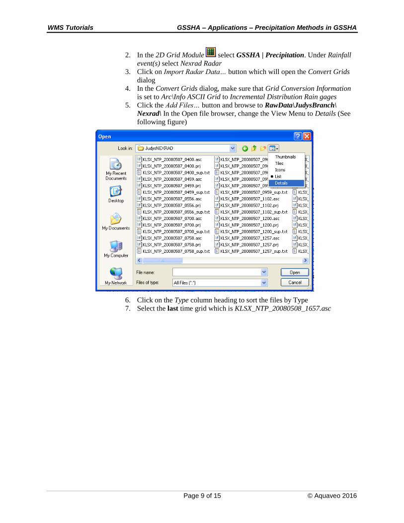
2. In the 2D Grid Module select GSSHA | Precipitation. Under Rainfall

event(s) select Nexrad Radar

3. Click on Import Radar Data… button which will open the Convert Grids

dialog

4. In the Convert Grids dialog, make sure that Grid Conversion Information

is set to Arc\Info ASCII Grid to Incremental Distribution Rain gages

5. Click the Add Files… button and browse to RawData\JudysBranch\

Nexrad\ In the Open file browser, change the View Menu to Details (See

following figure)

6. Click on the Type column heading to sort the files by Type

7. Select the last time grid which is KLSX_NTP_20080508_1657.asc



8. Hold the Shift key and select the starting time grid which is

KLSX_NTP_20080507_1200.asc

9. Click Open

10. In the Convert Grids dialog, toggle on the option Convert inches to

millimeters (if it is not already on)

11. Toggle on Create 2D grid rainfall dataset option.

12. Change the Starting date to 05\07\2008 and the Starting time to 12:00:00

PM.

13. Make sure that the time interval is 1 hour (60 min) (See the following

figure)



14. Click OK to save the grid file. It will take some time to create the gages for

the NEXRAD rainfall method.

15. After a couple of minutes the conversion process will complete and a

summary file will open up (Following figure) showing the date\time and

rainfall depth (mm) at each time interval.

16. Review and close the summary file



Many gages covering the watershed and a network of polygons joining the gages is now

visible. Notice a new Gridded Rainfall Gages coverage in the coverage tree.

17. The GSSHA Precipitation dialog will appear after the completion of the

conversion process. Toggle on the Gridded Rainfall Gages option and

click OK.

18. In the GSSHA precipitation dialog make sure to toggle off the Rain Gage

coverage and the change the interpolation method back to IDW.

19. The WMS window should look similar to the following figure.



6.9 Visualizing Meteorological Data

Before continuing, let us visualize the gridded rainfall data.

1. Toggle off the display of Gridded Rainfall Gages by unselecting it in the

project explorer.

2. Right-click on Rainfall Cumulative on the data tree under 2D Grid Data

and select Contour Options…Select Color Fill for the Contour Method.

Click OK

3. With the down arrow key on the keyboard, step through the time steps in

the properties window on the right sidebar to see how the precipitation

varies.

There are two rainfall datasets, one is incremental and the other is cumulative. View the

incremental rainfall dataset in the same way the cumulative dataset was viewed.

Whichever dataset is selected will be used to create the film loop.

4. In 2D Grid Module select Data | Film Loop…

5. Select the option to Create New Filmloop and specify the folder the

animation will be saved (Personal\Precipitation/precip.avi), check off the

option to Export to KMZ (Google Earth) and click Next

6. Toggle on either (Rainfall Cumulative) or (Rainfall Incremental) and

toggle off all other datasets.

7. Toggle off the option to write to KMZ file.

8. Toggle off the option to Write 2D scattered Dataset to KMZ file. See the

following figure



9. Click Next

10. Click Finish. WMS will now a few moments to create and save the

animation file. The animation will start playing as soon as the saving

process is complete.


The NEXRAD rainfall has been imported into GSSHA and copied the data into the

Gridded Rainfall Gages coverage. Next save and run the model.


2. Save it as Personal\Precipitation\nexrad.prj.


6.11 Visualization


2. With the Select Hydrographs tool selected, double-click on the

hydrograph icon to view the runoff hydrograph at the watershed outlet

3. For comparison, export the hydrograph ordinates and copy\paste in the

spreadsheet Tables\RainfallMethods.xls under the column NEXRAD.

4. See the difference in the outlet flow hydrograph in using different

precipitation methods.

5. Export the animations to Google Earth (Optional).

6.12 Summary

Open up the comparison spreadsheet and compare the results from different precipitation

methods.

v. 10 - aquaveowmstutorials-10.1.aquaveo.com/49 gssha-applications-precipitation.pdf · 6.4 using...

Documents