v-600 operation - university of california, irvinedmitryf/manuals/v-670 user guide.pdf · i preface...

P/N:0302-7420A September 2006

V-600 Operation

JASCO V-600 for Windows

Software Manual

i

Preface This instruction manual serves as a guide for using this instrument. It is intended to instruct first-time users on how to properly use the instrument, and to serve as a reference for experienced users. Before using the instrument, read this instruction manual carefully, and make sure you fully understand its contents. This manual should be easily accessible to the operator at all times during instrument operation. When not using the instrument, keep this manual stored in a safe place. Should this instruction manual be lost, order a replacement from your local JASCO distributor. Note: With this software you can use the same graphic user interface to analyze a wide variety

of data from various spectroscopic instruments. This manual explains all the functions offered by this software using data from a JASCO spectrometer. We have tried to ensure that all functions are explained clearly for users of any JASCO instrument compatible with this software, but if you cannot find an explanation for a specific function please contact your local JASCO representative.

ii

Servicing Contact your local JASCO distributor for instrument servicing. In addition, contact your JASCO distributor before moving the instrument to another location. Consumable parts should be ordered according to part number from your local JASCO distributor. If a part number is unknown, give your JASCO distributor the model name and serial number of your instrument. Do not return contaminated products or parts that may constitute a health hazard to JASCO employees.

Notices (1) JASCO shall not be held liable, either directly or indirectly, for any consequential damage incurred as a

result of product use.

(2) Prohibitions on the use of JASCO software

• Copying software for purposes other than backup • Transfer or licensing of the right to use software to a third party • Disclosure of confidential information regarding software • Modification of software • Use of software on multiple workstations, network terminals, or by other methods (not

applicable under a network licensing agreement concluded with JASCO) (3) The contents of this manual are subject to change without notice for product improvement.

(4) This manual is considered complete and accurate at publication.

(5) This manual does not guarantee the validity of any patent rights or other rights.

(6) If a JASCO software program has failed causing an error or improper operation, this may be caused by a conflict from another program operating on the PC. In this case, take corrective action by uninstalling the conflicting product(s).

(7) In general, company names and product names are trademarks or registered trademarks of the respective companies.

(8) JASCO and the JASCO logo are registered trademarks of JASCO Corporation

© JASCO Corporation, 2006. All rights reserved. Printed in JAPAN.

iii

Limited Warranty Products sold by JASCO, unless otherwise specified, are warranted for a period of one year from the date of shipment to be free of defects in materials and workmanship. If any defects in the product are found during this warranty period, JASCO will repair or replace the defective part(s) or product free of charge. THIS WARRANTY DOES NOT APPLY TO DEFECTS RESULTING FROM THE FOLLOWING: 1) IMPROPER OR INADEQUATE INSTALLATION 2) IMPROPER OR INADEQUATE OPERATION, MAINTENANCE, ADJUSTMENT OR

CALIBRATION 3) UNAUTHORIZED MODIFICATION OR MISUSE 4) USE OF CONSUMABLE PARTS NOT SUPPLIED BY AN AUTHORIZED JASCO DISTRIBUTOR 5) CORROSION DUE TO THE USE OF IMPROPER SOLVENTS, SAMPLES, OR DUE TO

SURROUNDING GASES 6) ACCIDENTS BEYOND JASCO'S CONTROL, INCLUDING NATURAL DISASTERS 7) CONSUMABLES AND PARTS OF WHICH WARRANTY PERIOD IS SPECIFIED OTHERWISE. THE WARRANTY FOR ALL PARTS SUPPLIED AND REPAIRS PROVIDED UNDER THIS WARRANTY EXPIRES ON THE WARRANTY EXPIRATION DATE OF THE ORIGINAL PRODUCT. FOR INQUIRIES CONCERNING REPAIR SERVICE, CONTACT YOUR JASCO DISTRIBUTOR AFTER CONFIRMING THE MODEL NAME AND SERIAL NUMBER OF YOUR INSTRUMENT. JASCO Corporation 2967-5, Ishikawa-cho, Hachioji-shi Tokyo 192-8537, JAPAN

iv

Contents

Preface ............................................................................................................................................................. i

Servicing .........................................................................................................................................................ii

Notices ............................................................................................................................................................ii

Limited Warranty ..........................................................................................................................................iii

Contents ......................................................................................................................................................... iv

1 Introduction .............................................................................................................................................. 1

1.1 Contents of this Manual ...................................................................................................... 1

1.2 Description of this Manual and the Notation Used ........................................................... 3

1.3 Overview of [Spectra Manager].......................................................................................... 4

2 Starting and Exiting Programs and [Spectra Manager] Menu Reference ............................................. 6

2.1 Startup .................................................................................................................................. 6 2.1.1 Turning ON the Spectrophotometer .................................................................................. 6 2.1.2 PC and Windows Startup and V-600 Series Registration.................................................. 7 2.1.3 Starting the [Spectra Manager] Program ......................................................................... 12 2.1.4 Components of the Program Screen ................................................................................ 14

2.2 Exiting ................................................................................................................................. 16 2.2.1 Exiting the Program......................................................................................................... 16 2.2.2 Shutting Off Power to the PC and Spectrophotometer .................................................... 16

2.3 [Spectra Manager] Menu Reference ................................................................................ 17

3 Accessory Auto Detection Reference...................................................................................................... 19

3.1 Tip When Connecting Auto Detection Accessories......................................................... 19

3.2 Registering Accessories ..................................................................................................... 20 3.2.1 Method for Registering Auto Detect Accessories ........................................................... 20 3.2.2 Method for Registering Non Auto Detection Accessories .............................................. 20

3.3 Registering Run Applications ........................................................................................... 23

3.4 Operating Auto Detection Accessories ............................................................................. 24 3.4.1 When Starting the Spectra Manager ................................................................................ 24

3.4.1.1 When a Single Run Application is Registered........................................................ 24 3.4.1.2 When Multiple Run Applications are Registered ................................................... 24

3.4.2 When a Measurement Application is Running................................................................ 25 3.4.2.1 When an Auto Detection Accessory is Attached .................................................... 25 3.4.2.2 When an Auto Detection Accessory is Removed ................................................... 27

3.5 Manually Detecting Accessories ....................................................................................... 28

3.6 Setting Parameters at Startup .......................................................................................... 28

4 Introduction to Spectra Measurement ................................................................................................... 29

4.1 Introduction to the [Spectra Measurement] Program.................................................... 29

4.2 Overview of the [Spectra Measurement] Program......................................................... 29

v

4.3 Setting Measurement Parameters .................................................................................... 30

4.4 Baseline Measurement....................................................................................................... 35

4.5 Sample Measurement ........................................................................................................ 36

4.6 Saving Spectra.................................................................................................................... 38

4.7 Printing the Measurement Result..................................................................................... 39

4.8 Shutting Down the Instrument ......................................................................................... 39

5 Introduction to the Quantitative Measurement Program...................................................................... 40

5.1 Overview of the Quantitative Measurement Program ................................................... 40

5.2 Quantitative Analysis Program ........................................................................................ 41

5.3 Overview of Quantitative Measurement Operations...................................................... 43

5.4 Using the [Quantitative Analysis] Program to Create a Calibration Curve and Perform a Quantitative Measurement.......................................................................................................... 45

5.4.1 Starting the [Quantitative Calibration] Program.............................................................. 45 5.4.2 Creating and Saving a Calibration Curve Template ........................................................ 46

5.4.2.1 Basic Mode ............................................................................................................. 46 5.4.2.2 Advanced Mode...................................................................................................... 52

5.4.3 Exiting [Quantitative Calibration] Program .................................................................... 58 5.4.4 Startup [Quantitative Analysis] Program......................................................................... 59 5.4.5 Opening Calibration Template ........................................................................................ 60 5.4.6 Creating Calibration Graph ............................................................................................. 61 5.4.7 Modifying Calibration Graph .......................................................................................... 63 5.4.8 Exiting Calibration Modification..................................................................................... 64 5.4.9 Measuring Samples of Unknown Concentrations ........................................................... 65 5.4.10 Saving Measurement Results ..................................................................................... 67 5.4.11 Printing Measurement Results ................................................................................... 68 5.4.12 Exiting [Quantitative Analysis] Program................................................................... 69

5.5 Creating a Calibration Curve with the [Quantitative Calibration] Program, and Performing a Quantitative Measurement with the [Quantitative Analysis] Program ............. 70

5.5.1 Startup the [Quantitative Calibration] program............................................................... 70 5.5.2 Creating and Saving the Calibration Template................................................................ 71 5.5.3 Creating Calibration Graph ............................................................................................. 71 5.5.4 Modifying Calibration Graph .......................................................................................... 73 5.5.5 Saving Measurement Results........................................................................................... 74 5.5.6 Exiting [Quantitative Calibration] Program .................................................................... 74 5.5.7 Startup [Quantitative Analysis] Program......................................................................... 75 5.5.8 Opening Calibration Curve File ...................................................................................... 75 5.5.9 Measuring Samples of Unknown Concentrations ........................................................... 77 5.5.10 Saving Measurement Results ..................................................................................... 78 5.5.11 Printing Measurement Results .................................................................................... 79 5.5.12 Exiting [Quantitative Analysis] Program.................................................................... 80

6 Quantitative Measurement Program Reference .................................................................................... 81

6.1 [Quantitative Calibration] Program Reference .............................................................. 81 6.1.1 [File(F)] Menu ................................................................................................................. 85

6.1.1.1 [New(N)…]............................................................................................................. 85

vi

6.1.1.2 [Open…] ............................................................................................................... 104 6.1.1.3 [Save] .................................................................................................................... 104 6.1.1.4 [Save As…]........................................................................................................... 105 6.1.1.5 [Export…]............................................................................................................. 106 6.1.1.6 [Open Template…] ............................................................................................... 107 6.1.1.7 [Save Template…]................................................................................................ 108 6.1.1.8 [Print…] ................................................................................................................ 108 6.1.1.9 [Print Preview…].................................................................................................. 109 6.1.1.10 [Print Item…]........................................................................................................ 110 6.1.1.11 [Print Setup…]...................................................................................................... 111 6.1.1.12 [Exit] ..................................................................................................................... 111

6.1.2 [Measure] Menu ............................................................................................................ 112 6.1.2.1 [Cancel]................................................................................................................. 112 6.1.2.2 [Sample]................................................................................................................ 112 6.1.2.3 [Blank] .................................................................................................................. 112 6.1.2.4 [Dark].................................................................................................................... 113 6.1.2.5 [Parameters…] ...................................................................................................... 114 6.1.2.6 [Preview]............................................................................................................... 114

6.1.3 [Control] Menu.............................................................................................................. 120 6.1.3.1 [Move Wavelength…] .......................................................................................... 120 6.1.3.2 [Optical Path] ........................................................................................................ 120 6.1.3.3 [Band Width] ........................................................................................................ 122 6.1.3.4 [Response] ............................................................................................................ 123 6.1.3.5 [Light Source] ....................................................................................................... 123 6.1.3.6 [Auto Zero] ........................................................................................................... 124 6.1.3.7 [Select Accessory…] ............................................................................................ 124

6.1.4 [Edit] Menu ................................................................................................................... 125 6.1.4.1 [Copy Graph] ........................................................................................................ 125 6.1.4.2 [Copy Table] ......................................................................................................... 125 6.1.4.3 [Delete] ................................................................................................................. 125 6.1.4.4 [Delete All] ........................................................................................................... 125

6.1.5 [View] Menu ................................................................................................................. 126 6.1.5.1 [Decimal Point…]................................................................................................. 126 6.1.5.2 [Information Bar] .................................................................................................. 126 6.1.5.3 [Tool Bar] ............................................................................................................. 126 6.1.5.4 [Status Bar] ........................................................................................................... 126 6.1.5.5 [Customize Toolbar…] ......................................................................................... 127 6.1.5.6 [Calibration Graph]............................................................................................... 129

6.1.6 [Settings] Menu ............................................................................................................. 134 6.1.6.1 [Default Template…]............................................................................................ 134

6.1.7 [Help] Menu .................................................................................................................. 134 6.1.7.1 [About…].............................................................................................................. 134

6.2 [Quantitative Measurement] Program Reference......................................................... 135 6.2.1 [File] Menu.................................................................................................................... 139

6.2.1.1 [New…] ................................................................................................................ 139 6.2.1.2 [Open …] .............................................................................................................. 140 6.2.1.3 [Save] .................................................................................................................... 141 6.2.1.4 [Save As …].......................................................................................................... 141 6.2.1.5 [Export…]............................................................................................................. 142

vii

6.2.1.6 [Print…] ................................................................................................................ 143 6.2.1.7 [Print Preview…].................................................................................................. 143 6.2.1.8 [Print Item…]........................................................................................................ 144 6.2.1.9 [Print Setup…]...................................................................................................... 145 6.2.1.10 [Exit] ..................................................................................................................... 145

6.2.2 [Measure] Menu ............................................................................................................ 146 6.2.2.1 [Cancel]................................................................................................................. 146 6.2.2.2 [Sample]................................................................................................................ 146 6.2.2.3 [Blank] .................................................................................................................. 147 6.2.2.4 [Dark].................................................................................................................... 148 6.2.2.5 [Parameters…] ...................................................................................................... 149 6.2.2.6 [Exit Modification] ............................................................................................... 149

6.2.3 [Control] Menu.............................................................................................................. 149 6.2.3.1 [Move Wavelength…] .......................................................................................... 149 6.2.3.2 [Optical Path] ........................................................................................................ 150 6.2.3.3 [Auto Zero] ........................................................................................................... 151 6.2.3.4 [Select Accessory …] ........................................................................................... 151

6.2.4 [Edit] Menu ................................................................................................................... 152 6.2.4.1 [Copy Graph] ........................................................................................................ 152 6.2.4.2 [Copy Table] ......................................................................................................... 152 6.2.4.3 [Delete] ................................................................................................................. 152 6.2.4.4 [Delete All] ........................................................................................................... 152 6.2.4.5 [Comment…] ........................................................................................................ 153

6.2.5 [View] Menu ................................................................................................................. 153 6.2.5.1 [Decimal Point…]................................................................................................. 153 6.2.5.2 [Information bar]................................................................................................... 154 6.2.5.3 [Tool bar] .............................................................................................................. 154 6.2.5.4 [Status bar] ............................................................................................................ 154 6.2.5.5 [Customize Toolbar…] ......................................................................................... 154 6.2.5.6 [Calibration Graph]............................................................................................... 156

6.2.6 [Settings] Menu ............................................................................................................. 161 6.2.6.1 [Default Parameters…] ......................................................................................... 161

6.2.7 [Help] Menu .................................................................................................................. 161 6.2.7.1 [About…].............................................................................................................. 161

7 [Spectra Measurement] Program Reference........................................................................................ 162

7.1 [File] Menu ....................................................................................................................... 166 7.1.1 [Save As…] ................................................................................................................... 166 7.1.2 [Analysis Send].............................................................................................................. 166 7.1.3 [Open Parameters…] ..................................................................................................... 167 7.1.4 [Save Parameters…] ...................................................................................................... 168 7.1.5 [Open Baseline…] ......................................................................................................... 169 7.1.6 [Save Baseline ...] .......................................................................................................... 171 7.1.7 [Open Dark Spectrum…]............................................................................................... 172 7.1.8 [Save Dark Spectrum] ................................................................................................... 174 7.1.9 [Exit].............................................................................................................................. 174

7.2 [Measure] Menu ............................................................................................................... 175 7.2.1 [Cancel] ......................................................................................................................... 175 7.2.2 [Sample] ........................................................................................................................ 175

viii

7.2.3 [Baseline]....................................................................................................................... 176 7.2.4 [Dark] ............................................................................................................................ 176 7.2.5 [Parameters…]............................................................................................................... 177

7.2.5.1 [General] tab ......................................................................................................... 177 7.2.5.2 [Control] tab.......................................................................................................... 184 7.2.5.3 [Information] tab................................................................................................... 187 7.2.5.4 [Data] tab .............................................................................................................. 188

7.2.6 [Preview…] ................................................................................................................... 189

7.3 [Control] Menu................................................................................................................. 189 7.3.1 [Move Wavelength…]................................................................................................... 189 7.3.2 [Optical Path]................................................................................................................. 190 7.3.3 [Band Width] ................................................................................................................. 191 7.3.4 [Response] ..................................................................................................................... 192 7.3.5 [Light Source]................................................................................................................ 192 7.3.6 [Auto Zero] .................................................................................................................... 193 7.3.7 [Select Accessory…] ..................................................................................................... 193

7.4 [View] Menu ..................................................................................................................... 194 7.4.1 [Scale…]........................................................................................................................ 194 7.4.2 [Pattern…] ..................................................................................................................... 195 7.4.3 [Font…] ......................................................................................................................... 196 7.4.4 [Gridlines…].................................................................................................................. 197 7.4.5 [Style…] ........................................................................................................................ 198 7.4.6 [Overlay]........................................................................................................................ 198 7.4.7 [Decimal Point…].......................................................................................................... 199 7.4.8 [Information Bar]........................................................................................................... 199 7.4.9 [Toolbar]........................................................................................................................ 199 7.4.10 [Status bar] ................................................................................................................ 199 7.4.11 [Customize Toolbar…] ............................................................................................. 200

7.5 [Settings] Menu ................................................................................................................ 202 7.5.1 [Default Parameters…].................................................................................................. 202

7.6 Help] Menu....................................................................................................................... 202 7.6.1 [About] .......................................................................................................................... 202

8 [Time course measurement] Program Reference ................................................................................ 203

8.1 [File] Menu ....................................................................................................................... 206 8.1.1 [Save Data…] ................................................................................................................ 206 8.1.2 [Analysis Send].............................................................................................................. 206 8.1.3 [Open Parameters…] ..................................................................................................... 207 8.1.4 [Save Parameters…] ...................................................................................................... 208 8.1.5 [Exit].............................................................................................................................. 208

8.2 [Measure] Menu ............................................................................................................... 209 8.2.1 [Cancel] ......................................................................................................................... 209 8.2.2 [Sample] ........................................................................................................................ 209 8.2.3 [Blank]........................................................................................................................... 210 8.2.4 [Dark] ............................................................................................................................ 210 8.2.5 [Parameters…]............................................................................................................... 211

8.2.5.1 [General] tab ......................................................................................................... 211 8.2.5.2 [Control] tab.......................................................................................................... 215

ix

8.2.5.3 [Information] tab................................................................................................... 217 8.2.5.4 [Data] tab .............................................................................................................. 218

8.2.6 [Preview…] ................................................................................................................... 219

8.3 [Control] Menu................................................................................................................. 220 8.3.1 [Move Wavelength…]................................................................................................... 220 8.3.2 [Optical Path]................................................................................................................. 220 8.3.3 [Band Width] ................................................................................................................. 221 8.3.4 [Response] ..................................................................................................................... 223 8.3.5 [Light Source...]............................................................................................................. 223 8.3.6 [Auto Zero] .................................................................................................................... 224 8.3.7 [Select Accessory…] ..................................................................................................... 224

8.4 [View] Menu ..................................................................................................................... 225 8.4.1 [Scale…]........................................................................................................................ 225 8.4.2 [Pattern…] ..................................................................................................................... 226 8.4.3 [Font…] ......................................................................................................................... 227 8.4.4 [Gridlines…].................................................................................................................. 228 8.4.5 [Style…] ........................................................................................................................ 229 8.4.6 [Decimal Point…].......................................................................................................... 230 8.4.7 [Information Bar]........................................................................................................... 230 8.4.8 [Toolbar]........................................................................................................................ 230 8.4.9 [Status Bar] .................................................................................................................... 230 8.4.10 [Customize Toolbar…] ............................................................................................ 231


8.6 [Help] Menu...................................................................................................................... 233 8.6.1 [About…] ...................................................................................................................... 233

9 [Fixed Wavelength Measurement] Program Reference ...................................................................... 234

9.1 [File] Menu ....................................................................................................................... 237 9.1.1 [New]............................................................................................................................. 237 9.1.2 [Open…]........................................................................................................................ 237 9.1.3 [Save]............................................................................................................................. 237 9.1.4 [Save As…] ................................................................................................................... 238 9.1.5 [Export…]...................................................................................................................... 239 9.1.6 [Open Parameters…] ..................................................................................................... 240 9.1.7 [Save Parameters…] ...................................................................................................... 241 9.1.8 [Print…]......................................................................................................................... 241 9.1.9 [Print Preview…]........................................................................................................... 242 9.1.10 [Print Item…] ............................................................................................................ 243 9.1.11 [Print Setup…] .......................................................................................................... 244 9.1.12 [Exit] ......................................................................................................................... 244

9.2 [Measure] Menu ............................................................................................................... 245 9.2.1 [Cancel] ......................................................................................................................... 245 9.2.2 [Sample] ........................................................................................................................ 245 9.2.3 [Blank]........................................................................................................................... 245 9.2.4 [Dark] ............................................................................................................................ 246 9.2.5 [Parameters…]............................................................................................................... 247

9.2.5.1 [General] tab ......................................................................................................... 247

x

9.2.5.2 [Control] tab.......................................................................................................... 251 9.2.5.3 [Sheet] tab ............................................................................................................. 253

9.2.6 [Preview…] ................................................................................................................... 254

9.3 [Control] Menu................................................................................................................. 255 9.3.1 [Move Wavelength…]................................................................................................... 255 9.3.2 [Optical path…]............................................................................................................. 255 9.3.3 [Band Width] ................................................................................................................. 257 9.3.4 [Response] ..................................................................................................................... 258 9.3.5 [Light Source…]............................................................................................................ 258 9.3.6 [Auto Zero] .................................................................................................................... 259 9.3.7 [Select Accessory…] ..................................................................................................... 259

9.4 [Edit] Menu....................................................................................................................... 260 9.4.1 [Copy]............................................................................................................................ 260 9.4.2 [Copy All]...................................................................................................................... 260 9.4.3 [Delete] .......................................................................................................................... 260 9.4.4 [Delete All] .................................................................................................................... 260 9.4.5 [Comment…]................................................................................................................. 261

9.5 [View] Menu ..................................................................................................................... 261 9.5.1 [Decimal Point] ............................................................................................................. 261 9.5.2 [Information Bar]........................................................................................................... 262 9.5.3 [Toolbar]........................................................................................................................ 262 9.5.4 [Status Bar] .................................................................................................................... 262 9.5.5 [Customize Toolbar…].................................................................................................. 262


9.7 [Help] Menu...................................................................................................................... 264 9.7.1 [About…] ...................................................................................................................... 264

10 [Abs/%T Meter] Program Reference.................................................................................................... 265

10.1 [Measure] Menu ............................................................................................................... 268 10.1.1 [Blank]....................................................................................................................... 268 10.1.2 [Dark] ........................................................................................................................ 268 10.1.3 [Parameters…] .......................................................................................................... 269

10.1.3.1 [General] tab ......................................................................................................... 269 10.1.3.2 [Control] tab.......................................................................................................... 271

10.1.4 [Preview…] ............................................................................................................... 272 10.1.5 [Exit] ......................................................................................................................... 272

10.2 [Control] Menu................................................................................................................. 273 10.2.1 [Move Wavelength…]............................................................................................... 273 10.2.2 [Optical Path…] ........................................................................................................ 273 10.2.3 [Band Width]............................................................................................................. 274 10.2.4 [Response]................................................................................................................. 276 10.2.5 [Light Source…] ....................................................................................................... 276 10.2.6 [Auto Zero]................................................................................................................ 277 10.2.7 [Select Accessory…]................................................................................................. 277

10.3 [View] Menu ..................................................................................................................... 278 10.3.1 [View Mode] ............................................................................................................. 278

xi

10.3.2 [Graph View] ............................................................................................................ 280 10.3.2.1 [Scale…] ............................................................................................................... 280 10.3.2.2 [Pattern...] ............................................................................................................. 281 10.3.2.3 [Font] .................................................................................................................... 281 10.3.2.4 [Gridlines…]......................................................................................................... 283 10.3.2.5 [Style…]................................................................................................................ 283

10.3.3 [Decimal Point…] ..................................................................................................... 284 10.3.4 [Tolerance Level…] .................................................................................................. 285 10.3.5 [Information Bar] ...................................................................................................... 286 10.3.6 [Toolbar] ................................................................................................................... 286 10.3.7 [Status Bar]................................................................................................................ 286 10.3.8 [Customize Toolbar…] ............................................................................................. 287

10.4 [Help] Menu...................................................................................................................... 288 10.4.1 [About…] .................................................................................................................. 288

1

1 Introduction This section describes how to use this manual, the rules of notation, windows configuration and special terms. Read this section first of all.

1.1 Contents of this Manual This section describes the structure of this manual and how to use it. This manual consists of 10 sections including this section. An explanation of each section is indicated below. In this manual, Microsoft Windows is referred to simply as “Windows” and “Personal Computer” has been shortened to “PC”. Note: For information about the [Validation], [Spectra Analysis] and [Jasco Canvas]

programs, please refer to the separate “Validation”, “JASCO Canvas Program” and “Spectra Analysis” manuals.

1. Introduction This section describes how to use this manual, the rules of notation and gives an overview of this program. Read this section first of all. 2. Startup and Shutdown of Program, Reference of [Spectra Manager] This section describes how to turn on the spectrophotometer and the PC, how to start up Windows and other programs, how to exit programs and how to turn off the PC and the spectrophotometer. First-time users should familiarize themselves with the system startup and shutdown procedures. For details on program operation, refer to Section 3 onwards. In addition, menu references for the [Spectra Manager] program are described. 3. Accessory Detection Reference This section describes how to register accessories used by the spectrophotometer as well as how to register and operate the start application during accessory detection. 4. Introduction to the [Spectra Measurement] Program In this section, a simple specific example of using the spectra measurement program is given. Those unfamiliar with the operation of Windows and first-time users of the spectrophotometer should follow the procedures described in this section to get a general overview of how to operate the spectrophotometer. 5. Introduction to the [Quantitative Measurement] Program In this section, a simple specific example of using the quantitative measurement program is given.

2

Those unfamiliar with the operation of Windows and first-time users of the spectrophotometer should follow the procedures described in this section to get a general overview of how to operate the spectrophotometer. 6 - 10. Measurement Program Menu Reference These sections contain measurement program menu references for quantitative measurements, spectral measurements, time course measurements and the like. Read the relevant sections as required.

3

1.2 Description of this Manual and the Notation Used Spectra Manager is an application program that runs on the Windows operating system, and thus requires a basic knowledge of Windows operations. This manual does not explain how to open menus, select commands and copy files. If you are a first-time user of Windows, familiarize yourself with the Windows operating system by referring to the operation manuals for the Windows operating system. The following notational conventions are used throughout this manual. General Notation Notation Meaning [Measurement] menu [Parameters...] command

Names of menus, commands and text boxes are enclosed in square brackets ‘[ ]’, followed by a description indicating whether the function is a menu, command, text box, etc.

<OK>, <Cancel> Names of buttons are enclosed in angular brackets ‘< >’. Keyboard Operations Notation Meaning Shift CTRL The name of the key is enclosed by a square, and shown in boldface. Alt , F Keys that are to be pressed in succession are separated by commas. In

the example shown on the left, the Alt key is to be pressed and released, followed by the F key.

Shift + → Keys that are pressed simultaneously are joined by "plus" signs. In the example shown on the left, press the → key while holding down the Shift key.

Mouse Operations Notation Meaning Point Move the mouse pointer to the specified item. Click Quickly press and release the mouse button. Double-click Click the mouse button twice in rapid succession. Drag Point to an item, click and hold down the mouse button. Move the

mouse with the button held down, and release the button when the pointer is in the desired position.

4

1.3 Overview of [Spectra Manager] Spectra Manager refers to the entire suite of measurement/analysis and administrative programs for JASCO spectrophotometers. Specifically, the Spectra Manager is an application program that configures communication with the spectrophotometer and that starts up various measurement and analysis programs. Measurement programs for the ultraviolet visible near-infrared (UV-Vis-NIR) spectrophotometer, "validation" programs that check the performance of the spectrophotometer, and the "Spectra Analysis", "JASCO Canvas" and "Administrative Tools" programs are common programs used on a variety of spectrophotometers can be started from the UV-Vis-NIR spectrophotometer. Spectra measurement Controls the spectrophotometer and performs measurements. Validation Checks the performance of the spectrophotometer. Spectra analysis Displays, processes and prints the data obtained by spectral

measurement. JASCO canvas Used to format and print spectral data. Administrative tools Controls the administration of the instrument and software

including the assignment of user authority. Directions for using programs that are mainly related to measurements are explained in this manual. For information on using the spectrophotometer itself, please refer to the separate "Hardware Manual". For information on validation, refer to the separate "Validation Manual". For detailed information about spectral analysis, refer to the separate "Spectra Analysis Manual". For information about the JASCO Canvas refer to the separate "JASCO Canvas Manual", while for information about administrative tools, refer to the separate "Administrative Tools Manual". The following programs are registered in the [Spectra Manager] of the Model V-600 as standard. Measurement programs (1) [Quantitative measurement] program

This program creates a calibration curve by measuring a standard sample of known concentration according to the common quantitative analysis method and measures an unknown sample to determine its concentration.

(2) [Spectra measurement] program

This program obtains UV/VIS absorption spectra of a sample. The spectrum acquired using this program is automatically transferred to the [Spectra Analysis] program for analysis.

(3) [Time Course Measurement] program

This program is used to measure changes to a sample over time at a fixed wavelength. The spectrum acquired is transferred by this program to the [Spectra Analysis] program for analysis.

(4) [Fixed Wavelength Measurement] program

This program measures the absorbance or transmittance of a sample at a fixed wavelength. Up to eight wavelengths can be set and measured.

5

(5) [Abs/%T Meter] program

The Abs/%T program is used to monitor photometric values. It is useful when a simple photometric value readout is required.

(6) [Validation] program

The validation program is used to check the basic performance of the spectrophotometer. It conducts tests based on various official methods.

Note: Please refer to the separate [Validation Manual] for information about the validation

program. Analysis program (1) [Spectra Analysis] program

This program saves, prints, and processes (difference spectra, peak picking, smoothing, derivative, vertical axis conversion, etc.) spectrum data or time course data.

(2) [JASCO Canvas] program

Use this program to layout and print spectra, measurement parameters, comments, etc. It can also be used to create drawings and enter characters.

Note: Please refer to the separate [Spectra Analysis Program] for information on the analysis

program.

6

2 Starting and Exiting Programs and [Spectra Manager] Menu Reference

2.1 Startup 2.1.1 Turning ON the Spectrophotometer Turn ON the power switch on the right side of the spectrophotometer.

"Power"switch

Light source lid

"START"switch

Fixing screw

Sample chamber

Figure 2.1 Spectrophotometer (V-650/660/670)

Turn on the power (the Power indicator will light up). It takes about 5 minutes for the light source to stabilize. Wait until the light source has stabilized before starting measurement.

7

2.1.2 PC and Windows Startup and V-600 Series Registration Turn on the power to the PC and display and start Windows. When first connecting the V-600 series or when connecting a new V-600 series, the instrument must be registered on the PC. Start Administrative Tools, right click on the screen that displays [Instrument] and select [Register Instrument].

Figure 2.2 [Administrative Tools] Window

(1) Select the V-600 series control driver and click the <Next> button.

Figure 2.3 [Select Instrument Driver] Dialog

8

(2) Enter the instrument name, model name and serial no. and click the <Finish> button to register the instrument. Enter the desired instrument name and enter the model name and serial no. inscribed on the name plate on the left side panel of the spectrophotometer (see Fig. 2.4).

Figure 2.4 [Instrument Properties] Window

The name of the registered instrument is displayed in the right screen of the administrative tools program.

Figure 2.5 [Administrative Tools] Window

Upon completion of registering the instrument, exit the program.

9

(3) Restart the program and start administrative tools. Right-click on the registered instrument name and select “Properties” to display the window shown in Fig.2.6. First, check that the Model, Display Name, and Serial Number are displayed as below in the [General] tab.

Figure 2.6 [Properties] Dialog, [General] tab

(4) Select the [Cell Unit] tab to register accessories.

Refer to Chapter 3 for details.

10

(5) Select the [Adjustment] tab to make instrument adjustments.

Figure 2.7 [Properties] Dialog, [Adjustment] tab

Clicking the <Diagnostic…> button displays the [Diagnostic] dialog.

11

Use this dialog to confirm that the instrument is functioning correctly.

Figure 2.8 [Diagnostic] Dialog

If an error is displayed, contact your local JASCO distributor.

Note 1: If the light source has been replaced, reset the light source operating hours to zero by

clicking the <Exchange> button for the deuterium lamp or tungsten lamp (see Fig. 2.7). Note 2: The [Calibration] tab contains functions only for use by JASCO service personnel.

12

2.1.3 Starting the [Spectra Manager] Program (1) After starting Windows, double-click on the [JASCO Spectra Manager] icon located on the Windows

desktop. The window shown in Fig. 2.9 is displayed. Note: Spectra Manager can also be started by selecting [Start] - [All Programs] - [JASCO] -

[Spectra Manager] from the Windows Start menu.

Figure 2.9 [Spectra Manager] Window

13

(2) Start the [Spectra Measurement] program to perform measurement. Select [Spectra Measurement] from the [Instrument] list of Spectra Manager and double-click it. The Spectra Measurement program starts and the following window appears.

Figure 2.10 [Spectra Measurement] Window

14

2.1.4 Components of the Program Screen In this section, an example of a spectra analysis program screen is used to explain the displays that are used to operate the program. The names of the various components (windows and dialogues) are also shown. (1) The View Window

In Spectra Analysis, you can open multiple spectrum Views within the main program window. These views have no dedicated menu bar, toolbar, or status bar. The toolbar buttons and other Spectra Analysis components can be operated in the same way as in the program window for the active View window.

Figure 2.11 Spectra Analysis Windows

View

15

(2) Dialog Boxes Commands and items in menus with an ellipsis (...) at the end open a dialog when clicked. Usually, the dialog contains parameters that must be set. The [Scale Settings] dialog of the [View] menu is used as an example to explain the names, functions, as well as the operational rules of various sections of the dialog box. The [Scale Settings] dialog box indicated in Fig. 2.12 is displayed by selecting [View] - [Style] in the Spectra Analysis program. The names of various sections of the dialog box are indicated below.

Figure 2.12 [Scale Settings] Dialog

Command button

Check box

Text box Group

Option button The black dot (•) shows that an option has been selected.

Drop-down list

16

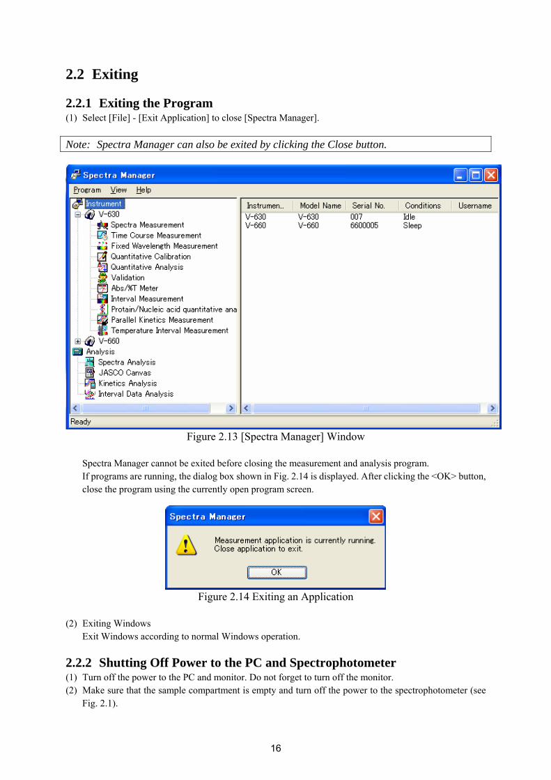
2.2 Exiting 2.2.1 Exiting the Program (1) Select [File] - [Exit Application] to close [Spectra Manager]. Note: Spectra Manager can also be exited by clicking the Close button.

Figure 2.13 [Spectra Manager] Window

Spectra Manager cannot be exited before closing the measurement and analysis program. If programs are running, the dialog box shown in Fig. 2.14 is displayed. After clicking the <OK> button, close the program using the currently open program screen.

Figure 2.14 Exiting an Application

(2) Exiting Windows

Exit Windows according to normal Windows operation. 2.2.2 Shutting Off Power to the PC and Spectrophotometer (1) Turn off the power to the PC and monitor. Do not forget to turn off the monitor. (2) Make sure that the sample compartment is empty and turn off the power to the spectrophotometer (see

Fig. 2.1).

17

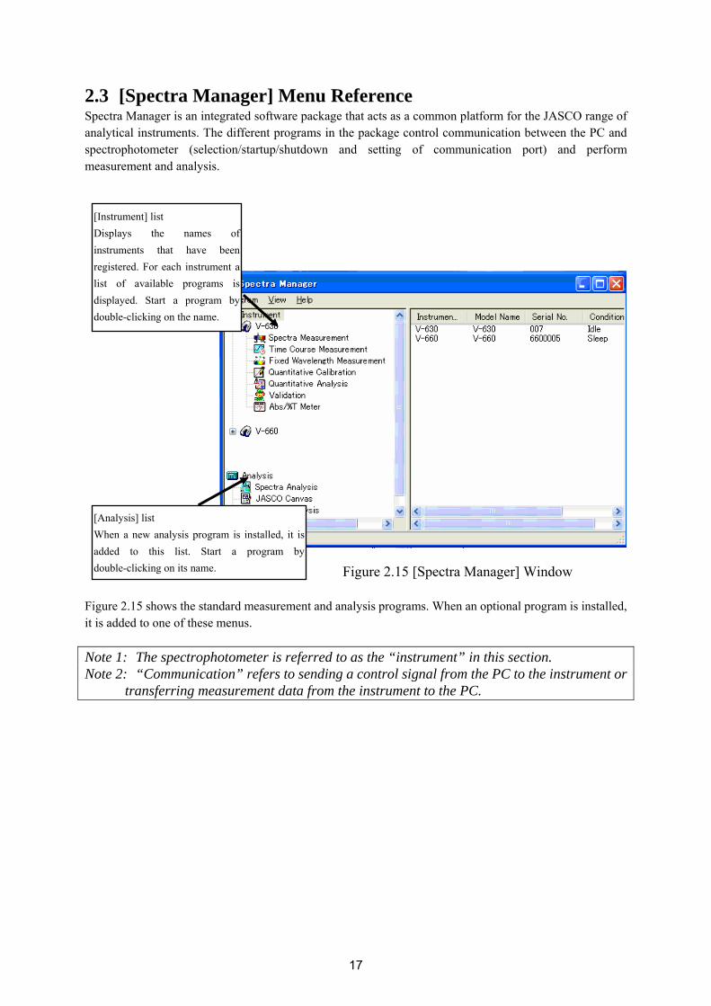
2.3 [Spectra Manager] Menu Reference Spectra Manager is an integrated software package that acts as a common platform for the JASCO range of analytical instruments. The different programs in the package control communication between the PC and spectrophotometer (selection/startup/shutdown and setting of communication port) and perform measurement and analysis.

Figure 2.15 [Spectra Manager] Window Figure 2.15 shows the standard measurement and analysis programs. When an optional program is installed, it is added to one of these menus. Note 1: The spectrophotometer is referred to as the “instrument” in this section. Note 2: “Communication” refers to sending a control signal from the PC to the instrument or

transferring measurement data from the instrument to the PC.

[Analysis] list When a new analysis program is installed, it is added to this list. Start a program by double-clicking on its name.

[Instrument] list Displays the names of instruments that have been registered. For each instrument a list of available programs is displayed. Start a program by double-clicking on the name.

18

Menu [Program] menu [Administrative Tool…] Starts the administrative tool. [Exit] Exits the [Spectra Manager] program. [Application] menu [Start] Initializes the spectrophotometer and starts communication (startup). This

takes about 2 minutes. The spectrophotometer starts automatically when the measurement program is started, so this operation is usually unnecessary.

[Open] Selects a measurement parameter file and starts the measurement program using the parameters.

[View] menu [Status bar] Sets show/hide of the status bar. [Folder] Displays the folder window. [Search] Displays the file search window. [Help] menu [Contents] Displays the contents window for help. [Topic] Displays the keywords window for help. [Version…] Displays the version information for the control program of the

spectrophotometer.

19

3 Accessory Auto Detection Reference The V600 series automatically detects accessories, and can display information on detected accessories and to automatically start the application registered to that accessory. Tips for connecting accessories, the method for registering the accessory being used, and the method for registering applications that start when the instrument recognizes an accessory, as well as operations performed when an accessory is detected are explained in this section.

3.1 Tip When Connecting Auto Detection Accessories The accessory for V-600 is automatically detected. The accessory information chip is installed in the accessory (shown in Fig 3.1). When the accessory information chip touches the accessory information contact, the accessory is detected. Please refer to the software manual of the spectrophotometer or the software manual for intelligent remote module type for details.

Figure 3.1 Accessory Detection Part

Accessory detection contact

Accessory information chip

20

3.2 Registering Accessories The method for registering accessories used by the spectrophotometer are explained in this section. 3.2.1 Method for Registering Auto Detect Accessories (1) Confirm that the instrument is turned on and that the Spectra Manager program is open. (2) Place the auto detection accessory in the sample compartment and the accessory name, accessory ID and

serial number are automatically registered. 3.2.2 Method for Registering Non Auto Detection Accessories (1) Start Administrative Tools and right click on the registered instrument name and then click Properties.

Figure 3.2 Administrative Tools

21

(2) The [Properties] dialog is displayed. Click the [Cell Unit] tab and select the accessory type to be registered in this dialog box.

Figure 3.3 [Properties] Window

Table 3.1 Accessory types Type Cell holder Cell changer Peristaltic sipper Vacuum sipper Temperature controller Reflectance measurement unit Integrating sphere Film holder Flow cell Optical fiber unit Fiber optics for external light source

22

(3) Click the <Add…> button to display the following dialog.

Figure 3.4 [Register Accessory] Dialog

(4) Select the model name and the accessory name is automatically inputted. Enter the serial No. and comment and click <OK> to register the accessory in the list.

Figure 3.5 [Properties] Dialog, [Cell Unit] tab

Accessory list

23

3.3 Registering Run Applications The method for registering applications that automatically run when the instrument detects an accessory is explained in this section. (1) Open the [Properties] dialog, select the [Cell Unit] tab and the screen shown above (Fig. 3.5) is

displayed.

(2) From the [Accessory List], select the accessory that is to be registered to a run application and then click the <Run Applications…> button.

(3) The [Select Applications] dialog is displayed. Select the application to be opened when the application is started and click the <OK> button to complete the registration of the accessory.

Note: Multiple applications can be selected. If no run applications are registered, then no applications will start automatically, even if the spectrophotometer detects an accessory.

Figure 3.6 [Select Applications] Window

24

3.4 Operating Auto Detection Accessories Note: If any applications display a dialog or message, do not connect or remove an auto

detection accessory. 3.4.1 When Starting the Spectra Manager Information about attaching auto detection accessories with a registered run application when Spectra Manager is started up or when the Spectra Manager screen is displayed when a measurement application is not running is given in this section. Note: Nothing is displayed if an accessory that is not linked to a run application is connected. 3.4.1.1 When a Single Run Application is Registered When an auto detection accessory is connected, the appropriate application starts automatically. 3.4.1.2 When Multiple Run Applications are Registered When an auto detection accessory is connected, a list of registered run applications is displayed (Fig. 3.7). Select the measurement application to use and click the <OK> button. The application will start automatically.

Figure 3.7 [Select Applications] Dialog

25

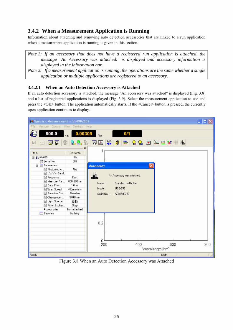
3.4.2 When a Measurement Application is Running Information about attaching and removing auto detection accessories that are linked to a run application when a measurement application is running is given in this section. Note 1: If an accessory that does not have a registered run application is attached, the

message "An Accessory was attached." is displayed and accessory information is displayed in the information bar.

Note 2: If a measurement application is running, the operations are the same whether a single application or multiple applications are registered to an accessory.

3.4.2.1 When an Auto Detection Accessory is Attached If an auto detection accessory is attached, the message "An accessory was attached" is displayed (Fig. 3.8) and a list of registered applications is displayed (Fig. 3.9). Select the measurement application to use and press the <OK> button. The application automatically starts. If the <Cancel> button is pressed, the currently open application continues to display.

Figure 3.8 When an Auto Detection Accessory was Attached

26

Figure 3.9 Display of Run Application

27

3.4.2.2 When an Auto Detection Accessory is Removed When an auto detection accessory is removed, the message "An accessory has been removed" is displayed and the accessory information in the information bar disappears.

Figure 3.10 When an Auto Detection Accessory is Removed

Information bar Accessory information

28

3.5 Manually Detecting Accessories When using a non-auto detection accessory, place it in the sample compartment and select [Select Accessory] in the [Control] menu of the application to be used. Figure 3.11 is displayed in the window. Select the application to be used and click the <OK> button. As in Section 3.4.2.1. “When an Accessory is Attached”, the “An accessory was attached” message is displayed and a list of registered applications is displayed.

Figure 3.11 [Select Accessory] Dialog

3.6 Setting Parameters at Startup The measurement conditions at startup when an accessory is detected can be set by the applications. For further details, please refer to the Menu Reference [Settings] menu - [Default Parameters…] for each application.

29

4 Introduction to Spectra Measurement This section describes how to use the [Spectra Measurement] program. The parameters are only described briefly in order to make the operation flow clear. Follow the procedures outlined below in order to become familiar with the operation of spectrophotometer. For more detailed information, see the [Spectra Measurement] program menu reference.

4.1 Introduction to the [Spectra Measurement] Program The specific procedures for starting the Spectra Measurement program, measuring the spectrum of holmium glass (a standard accessory), saving the measured spectrum and printing are described in this section.

4.2 Overview of the [Spectra Measurement] Program The Spectra Measurement Program is used to measure a sample spectrum under set measurement conditions. Setting measurement parameters Refer to Section 4.3 ↓

Baseline measurement Refer to Section 4.4 ↓

Sample measurement Refer to Section 4.5 ↓

Saving spectra Refer to Section 4.6 ↓

Printing results Refer to Section 4.7 ↓

Shutting down instrument Refer to Section 4.8

30

4.3 Setting Measurement Parameters (1) Select [Parameters…] from the [Measure] menu (or click the button). (2) The [Parameters] dialog is displayed (Fig. 4.1). The [General] tab is open by default in the Parameters

dialog. To change between the different dialogs, click the tabs at the top of the window. (3) The measurement conditions are set in the [General] tab as indicated below. The setting conditions for [Basic Mode] are used as an example here. To toggle between [Basic Mode] and [Advanced Mode], click the <Basic Mode > or <Advanced Mode > button.

Figure 4.1 [Parameters Basic] Dialog, [General] tab Note 1: The bandwidth for the V-630 is fixed at 1.5 nm. Note 2: The [NIR Band Width] setting shown in Fig. 4.1 is only valid for the V-670.

31

Photometric Mode %T Response Fast Bandwidth 2 nm (default setting) Scan 1000 nm/min (default setting) Start 900 nm End 200 nm Data Pitch 0.5 nm (default setting) Vertical Scale Auto Accumulation OFF Cycle Times 1

Setting the [Photometric mode] The [Photometric Mode] is a drop-down list box. Click the arrow to the right of the box to display the available modes. Click [%T] to set that photometric mode. Setting the [Response] The [Response] is a drop-down list box like [Photometric Mode]. Set [Response] to [Fast]. When [Response] is set in [Basic Mode], the optimal [Scan] and [Data Pitch] are determined automatically. Setting the [Start] and [End]. Input the long wavelength end [900 nm] into the [Start] text box and the short wavelength end [200 nm] into the [End] text box.

For example, to input [Start], click on that text box. The cursor appears in the text box, waiting for input. Delete the unrequired value and input the wavelength using the numeric keypad.

32

(4) Click on the [Control] tab to set the parameters as follows.

Figure 4.2 [Parameter Basic] Dialog, [Control] tab

Note: The [Grating/Detector] setting shown in Fig. 4.2 is for the V-670 only.

Baseline ON Light Source Changeover Wavelength

340 nm

Grating/Detector Changeover Wavelength

900 nm

33

(5) Click on the [Information] tab. Enter the [Sample Name], [Operator], [Division], and [Comment] as desired. The information entered here is saved as comment information together with the spectral data when the spectrum is saved. To display the [Information] dialog prior to taking a measurement, check the [Display the [Comment] dialog box before taking measurement] box.

Figure 4.3 [Parameters Basic] Dialog, [Information] tab

Sample Name Set as desired (maximum 63 characters). Operator Set as desired (maximum 63 characters). Division Set as desired (maximum 127 characters). Comment Set as desired (maximum 127 characters). Display the [Comment] dialog box before measurement

OFF

34

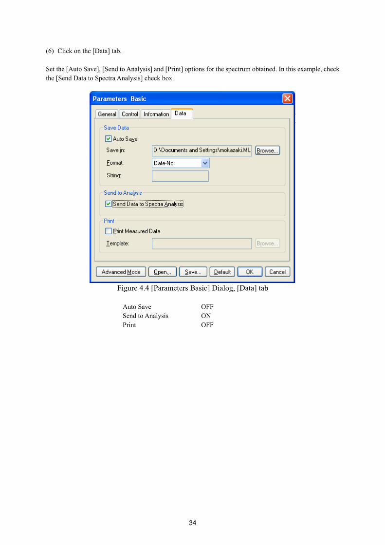
(6) Click on the [Data] tab. Set the [Auto Save], [Send to Analysis] and [Print] options for the spectrum obtained. In this example, check the [Send Data to Spectra Analysis] check box.

Figure 4.4 [Parameters Basic] Dialog, [Data] tab

Auto Save OFF Send to Analysis ON Print OFF

35

4.4 Baseline Measurement The baseline defines the absorbance 0 (or transmittance 100%) and is subtracted from the measurement result to give a correct sample spectrum (or is divided in the case of transmittance). The baseline characteristics are inherent to an instrument, but in an actual measurement they differ slightly depending on the measurement parameters, such as response, scanning speed and other settings. It is recommended to measure the baseline under the same conditions as the actual spectrum measurement conditions in order to obtain an accurate spectrum. Note: When an optional accessory is installed in the sample compartment, the light path

changes, making it necessary to remeasure the baseline.

(1) To perform baseline measurement, click [Measure] - [Baseline Measurement] (or click the button) to open the following dialog.

Select whether to use a blank sample or air for the baseline; this choice will differ depending on the sample. For the holmium glass measurement, air is used for the baseline. Confirm that the sample compartment is empty and start the baseline measurement. Clicking the <Measure> button will cause the measurement to start.

Figure 4.5 [Baseline Measurement] Dialog

(2) Starts a baseline measurement. Click the <Measure> button to start a measurement.

36

4.5 Sample Measurement (1) Once the baseline measurement is complete, insert the sample in the cell holder on the sample side (i.e. at

the front) of the sample compartment and close the door.

(2) Select the [Measure] - [Sample] menu (or click the button). Sample measurement starts and the progress of the measurement is displayed in the window (see Fig. 4.6).

Figure 4.6 [Spectra Measurement] Screen

After taking measurements, the [Spectra Analysis] program starts and the measured spectrum is displayed in the window. This window is called a View. Figure 4.7 shows an example of a measured spectrum that has not yet been saved (Title bar: “View <Memory-1>”). Note 1: If the Spectra Analysis program is already running, it does not appear on the front

window. Click [Spectra Analysis] on the Windows task bar to bring the program to the front.

Note2: Data is not transferred unless [Send to Analysis] is turned ON in the [Data] tab of the [Parameters] dialog. To enable automatic transfer of data, mark the [Send data to

Spectra Analysis] (or click the button) check box.

37

Figure 4.7 Spectra View (%T mode)

38

4.6 Saving Spectra In this section, the procedure for saving a spectrum using the [Spectra Analysis] program is described.

Note: The spectrum can also be saved from [File] - [Save Data] (or by clicking the button) in the Spectra Measurement program.

(1) Select [Save As…] from the [File] menu in the Spectra Analysis program to display the following dialog.

Figure 4.8 [Save Data] Dialog (2) [Save as type] is set to the format of [Standard Files (*.jws)] automatically. (3) Select the folder to save in from the [Save in] box. (4) Enter the filename in the [File name] field. Here, enter “holmium” as the filename. Note: Do not add an extension in the [File Name] field. (5) After entering the filename, click the <OK> button. The filename has the extension “.jws” added

(“Holmium.jws”), which is the standard file type. (6) The file is now saved.

After saving, the title bar of the View changes to “View (holmium.jws)”.

Note: Refer to the “Spectra Analysis” manual for more information about saving a spectrum.

39

4.7 Printing the Measurement Result The acquired spectrum can be printed on a printer. (1) Select [File] - [Print Setup…] to open the following dialog. The content of this dialog varies depending

on the printer.

Figure 4.9 [Print Setup] Dialog

(2) Select [File] - [Print] to print the spectrum.

Note: Refer to the “Spectra Analysis” manual for more information on printing.

4.8 Shutting Down the Instrument (1) Exiting the [Spectra Analysis] program

Select [File] - [Exit]. The [Spectra Analysis] window closes and the [Spectra Measurement] window appears.

Note: If there are unsaved spectra in the window, a warning message is displayed. Perform the

action recommended by the message. A message for each unsaved spectrum is displayed.

(2) Exiting the [Spectra Measurement] program

Select [File] - [Exit]. The [Spectra Measurement] window closes and the [Spectra Manager] window is displayed.

(3) Exiting the [Spectra Manager] program Select [Program] - [Exit].

(4) Exiting Windows

Exit Windows in accordance with Windows procedures. (5) Shutting off power to the PC and spectrophotometer

Turn off the power to the PC and monitor. Do not forget to turn off the monitor. Make sure that the sample compartment is empty and turn off the power to the spectrophotometer.

40

5 Introduction to the Quantitative Measurement Program The [Quantitative Calibration] and [Quantitative Analysis] programs are described in this section. The explanation of parameters is kept to a minimum; the focus of the explanation is on the flow of operations. First, prepare the standard sample to be quantitatively measured as well as the sample having unknown concentration. Follow the procedures described below to become familiar with using the spectrophotometer. See the relevant program's menu references for a more detailed explanation.

5.1 Overview of the Quantitative Measurement Program A simple explanation of the quantitative measurement method is first introduced in this section, followed by an explanation of the procedures for creating a calibration curve, measuring a sample of unknown concentration and saving and printing the results. The process flow is covered ranging from creation of the calibration curve to quantitative measurement, which can be done by either of the following two methods. (1) Quantitative measurement is performed after creating a calibration template using the [Quantitative

Calibration] program, loading the temperate using the [Quantitative Analysis] program and creating a calibration curve.

(2) Quantitative measurement is performed after creating a template, creating a calibration curve using the

[Quantitative Calibration] program, and loading the calibration curve file using the [Quantitative Analysis] program.

In (1), an accessory such as a multiple cell changer or an auto sampler is used and all operations from creation of the calibration curve to the quantitative measurement are performed using the [Quantitative Analysis] program. When this method is used, the calibration curve file and the quantitative measurement results cannot be saved separately, so if a single calibration curve is to be used multiple times for quantitative analysis, use method (2). Note 1: The calibration curve template means the measurement parameters. Note 2: The calibration curve file means the measurement parameters and the calibration

curve information. The following sections describes both methods (1) and (2).

41

5.2 Quantitative Analysis Program The Quantitative Analysis program is based on generally used analysis methods. (1) The following quantitative analysis methods are available. Choose the optimal method based on the

properties of the sample being measured. 1) No Base (1 wavelength quantitative analysis) (Refer to Fig. 5.1 (1))

Used for normal solution sample. 2) 1 Base (2 Wavelength Quantitative Analysis) (refer to Fig. 5.1 (2))

Used for a sample with a floating baseline. 3) 2 Base (3 Wavelength Quantitative Analysis) (refer to Fig. 5.1 (3))

Used for a sample with an inclined baseline. The following formula is used for 3-wavelength quantitative analysis. WL1 is the wavelength and E (1) the absorbance at that wavelength.

∆ Abs = E(1)- |WL1-WL2|・E(3)+|WL3-WL1|・E(2)

|WL3-WL2|

WL 1 WL 1 WL 2

D Abs D Abs

WL 1 WL 2 WL 3

E(2)

E(1)

E(3)

(1) (2) (3) 1-wavelength 2-wavelength 3-wavelength

(Peak) (Base 1) (Peak) (Peak) (Base 1) (Base2)

Figure 5.1 Quantitative Analysis Methods

42

(2) The optimum calibration curve can be selected from the modes shown in Fig.5.2.

Segmented line Logistic function Spline function

Proportional function Linear function Quadratic function Third-order function

Figure 5.2 Calibration Curve Mode Note: Those modes marked with a "*" can be selected to either pass through or not pass

through the origin. (3) The operator can select whether to use standard measurement data (set of concentration/absorbance) to

calculate the calibration curve.

**

*

43

5.3 Overview of Quantitative Measurement Operations (1) Quantitative measurement is performed after creating a template using the [Quantitative Calibration]

program, loading the temperate using the [Quantitative Analysis] program and creating the calibration curve.

Use this method when accessories such as a multiple cell changer or auto sampler are being used and all operations from the creation of the calibration curve to quantitative analysis are being done using the [Quantitative Analysis] program.

Starting the [Quantitative Calibration] program Refer to Section 5.4.1

↓

Creating and Saving the Calibration Curve Template Refer to Section 5.4.2 ↓

Exiting [Quantitative Calibration] program Refer to Section 5.4.3 ↓

Startup [Quantitative analysis] program Refer to Section 5.4.4 ↓

Opening a Calibration Curve Template Refer to Section 5.4.5 ↓

Creating a Calibration Graph Refer to Section 5.4.6 ↓

Modifying a Calibration Graph Refer to Section 5.4.7 ↓

Exiting Calibration Curve Editing Refer to Section 5.4.8 ↓

Measuring samples of unknown concentrations Refer to Section 5.4.9 ↓

Saving results Refer to Section 5.4.10 ↓

Printing results Refer to Section 5.4.11 ↓

Exiting [Quantitative analysis] program Refer to Section 5.4.12

44

(2) Quantitative measurement is performed after creating a template, creating a calibration curve, and loading the calibration curve using the [Quantitative Analysis] program.

Use this method when using a single calibration curve for multiple measurements.

Starting the [Quantitative Calibration] program Refer to Section 5.5.1

↓

Creating and Saving a Calibration Curve Template Refer to Section 5.5.2 ↓

Creating a Calibration Curve Graph Refer to Section 5.5.3 ↓

Editing a Calibration Curve Graph Refer to Section 5.5.4 ↓

Saving a Calibration Curve File Refer to Section 5.5.5 ↓

Exiting [Quantitative Calibration] program Refer to Section 5.5.6 ↓

Startup [Quantitative Analysis] program Refer to Section 5.5.7 ↓

Opening a Calibration Curve File Refer to Section 5.5.8 ↓

Measuring samples of unknown concentrations Refer to Section 5.5.9 ↓

Saving results Refer to Section 5.5.10 ↓

Printing results Refer to Section 5.5.11 ↓

Exiting [Quantitative Analysis] program Refer to Section 5.5.12

45

5.4 Using the [Quantitative Analysis] Program to Create a Calibration Curve and Perform a Quantitative Measurement Quantitative measurement is performed after creating a template using the [Quantitative Calibration] program, loading the template using the [Quantitative Analysis] program and creating a calibration curve. 5.4.1 Starting the [Quantitative Calibration] Program In the [Spectra Manager] window, double-click [Quantitative Calibration]. [Quantitative Calibration] program starts and the following window appears.

Figure 5.3 [Quantitative Calibration] Window

46

5.4.2 Creating and Saving a Calibration Curve Template

Select [File] - [New] (or click the button). The [Parameters Basic] dialog is displayed. Set the new calibration curve template using this dialog. There are two modes for creating a calibration curve template: Basic Mode and Advanced Mode. In Basic Mode, a minimum number of calibration curve template settings are available to the user, while in Advanced Mode, detailed measurement conditions, calibration graph and worksheet settings can be set to conform to the user's requirements. The method for creating a calibration curve template using these two modes is explained below. To toggle between Basic and Advanced modes, click either the [Basic Mode] or [Advanced Mode] buttons. 5.4.2.1 Basic Mode The dialog of basic mode has five tabs to set: Parameters, Calibration Graph, Control, Pass/Fail, Comment. These dialogs can be changed by clicking the tab for each dialog. (1) Click [File] - [New] to first display the [Parameters] tab.

Figure 5.4 [Parameters Basic] Dialog, [Parameters] tab

47

The following settings can be changed in the [Parameters] tab. Method No base (one wavelength)

(Set in accordance with the sample) Peak 500 nm (Set in accordance with the sample)

Response Medium

Note 1: The bandwidth for the V-630 is fixed at 1.5 nm. Note 2: The [NIR Band Width] is a parameter that is only displayed when using the V-670.

[Method] is a drop-down list box. Click the arrow to the right of the box to display the full list of options. Select the target [Method]. Next, enter the peak wavelength of the sample into the [Peak] text box. Delete the unrequired value and input the wavelength using the numeric keypad.

(2) Click on the [Calibration Graph] tab (see Fig. 5.5).

Figure 5.5 [Parameters Basic] Dialog, [Calibration Graph] tab

48

The following settings can be changed in the [Calibration Graph] tab.

Equation Proportional （Set in accordance with the sample） Unit (Set in accordance with the sample)

[Equation] is a drop-down list box. Click the arrow to the right of the box to display the full list of options. Click the target equation. Select the target [Unit] in the same manner.

Note: Double-click the [Unit] text box to input units freely. (3) Click on the [Control] tab (see Fig. 5.6).

Figure 5.6 [Parameters Basic] Dialog, [Control] tab

The following settings can be changed in the [Control] tab.

Light Source 340 nm

Note: The [Grating] setting is only valid for the V-670.

49

(4) Click on the [Pass/Fail] tab (see Fig. 5.7). The [Pass/Fail] tab sets the pass conditions for the quantitative measurement results for the concentration. In this example, the condition [0<= and <=1] is set.

Figure 5.7 [Parameters Basic] Dialog, [Pass/Fail] tab

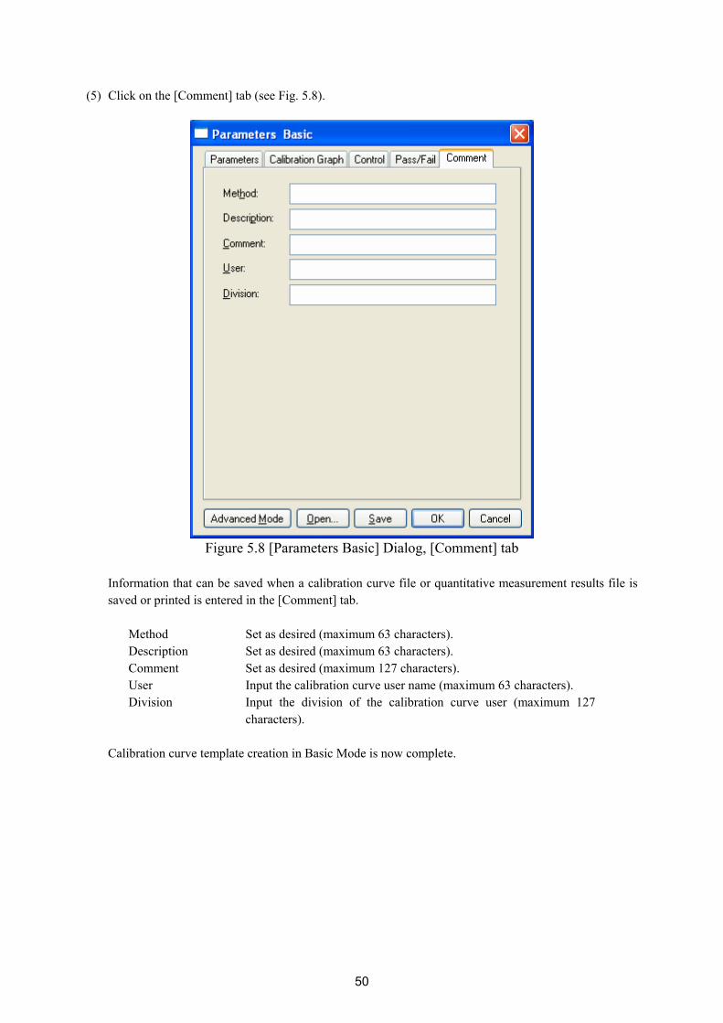
50

(5) Click on the [Comment] tab (see Fig. 5.8).

Figure 5.8 [Parameters Basic] Dialog, [Comment] tab

Information that can be saved when a calibration curve file or quantitative measurement results file is saved or printed is entered in the [Comment] tab.

Method Set as desired (maximum 63 characters). Description Set as desired (maximum 63 characters). Comment Set as desired (maximum 127 characters). User Input the calibration curve user name (maximum 63 characters). Division Input the division of the calibration curve user (maximum 127

characters).

Calibration curve template creation in Basic Mode is now complete.

51

Click the <Save> button to display the window in Fig. 5.9. Input the calibration curve template filename and click the <Save> button.

Figure 5.9 [Save Template] Dialog

After saving the template, click the <OK> button in the [Parameters Basic] dialog to close.

52

5.4.2.2 Advanced Mode The dialog of basic mode has six tabs to set: Parameters, Calibration Graph, Worksheet, Control, Pass/Fail, and Comment. These dialogs can be changed by clicking the tab for each dialog. (1) Select [File] - [New] to first display the [Parameters] tab.

Figure 5.10 [Parameters Advanced] Dialog, [Parameters] tab

The following settings can be changed in the [Parameters] tab.

Method No base (one wavelength) (set in accordance with the sample) Peak 500 nm (set in accordance with the sample) Response Medium Band Width 2 nm Cycle Times 1

Note 1: The bandwidth for the V-630 is fixed at 1.5 nm. Note 2: [NIR Band Width] can only be set for the V-670. If the V-670 is being used, [NIR Band

Width] will not affect measurements at 500 nm, and does not need to be set.

[Method] is a drop-down list box. Click the arrow to the right of the box to display the full list of options. Select the target [Method]. Next, input the peak wavelength of the sample into the [Peak] text box. Delete the unrequired value and input the wavelength using the numeric keypad.

53

[Response] is a drop-down list box. Click the arrow to the right of the box to display the full list of options. Clicking [Medium] sets the response to [Medium]. Set [Band Width] to [2.0 nm]. Input 1 for [Cycle Times].

(2) Click on the [Calibration Graph] tab (see Fig 5.11).

Figure 5.11 [Parameters Advanced] Dialog, [Calibration Graph] tab

The following settings can be changed in the [Calibration Graph] tab.

Measure Standard Selection Equation Proportional (set in accordance with the sample)

Unit (set in accordance with the sample)

For the [Calibration Method], select [Measure Standard] and select the desired [Equation]. Select the target [Unit] in the same manner.

Note: Double-click on the [Unit] text box to input units freely.

54

(3) Click the [Worksheet] tab. The worksheet used by the Quantitative Calibration program and the Quantitative Analysis program is created in the [Work Sheet] window. Widen the width of the [Parameters Advanced] dialog to display the entire [Work Sheet] window as shown in Fig. 5.12.

Select [Calibration] to show the window shown in Fig. 5.12. Select [Quantitative] to show the window shown in Fig. 5.13. The [Default] worksheet is set and used here, so there is no need to edit this item.

Figure 5.12 [Parameters Advanced] Dialog, [Work Sheet] tab (Calibration)

Figure 5.13 [Parameters Advanced] Dialog, [Word Sheet] tab (Quantitative)

55

Note: The [Calibration] worksheet cannot be edited once the standard sample measurement begins. The [Quantitative] worksheet cannot be edited once measurement of a sample of unknown concentration begins.

(4) Click on the [Control] tab (see Fig. 5.14).

Figure 5.14 [Parameters Advanced] Dialog, [Control] tab

The following settings can be changed in the [Control] tab

Light Source 340 nm External Source OFF Dark Correction OFF

Note: The [Grating] setting is only valid for the V-670.

56

(5) Click the [Pass/Fail] tab and the window shown in Fig. 5.15 is displayed. The pass conditions for the concentration from the quantitative analysis results obtained from the Quantitative Analysis program are set in the [Pass/Fail] tab. In this example, [0<= and <=1] is set.

Figure 5.15 [Parameters Advanced] Dialog, [Pass/Fail] tab

57

(6) Click on the [Comment] tab (see Fig. 5.16).

Figure 5.16 [Parameters Advanced] Dialog, [Comment] tab

Information that can be saved when a calibration curve file or quantitative measurement results file is saved or printed is entered in the [Comment] tab.

Method Set as desired (maximum 63 characters). Description Set as desired (maximum 63 characters). Comment Set as desired (maximum 127 characters). User Input the calibration curve username. (maximum 63 characters). Division Input the division of the calibration curve user. (maximum 127

characters).

Calibration curve template creation in [Advanced Mode] is now complete.

58

Clicking the <Save> button displays the window shown in Figure 5.17. Input the calibration curve template filename and click the <Save> button.


After saving the template, click the <OK> button on the <Parameters Advanced> dialog to close it. 5.4.3 Exiting [Quantitative Calibration] Program After creating and saving the calibration template, select [File] - [Exit].

Note: No warning message is displayed even if unsaved calibration templates are open.

59

5.4.4 Startup [Quantitative Analysis] Program Double-click [Quantitative Analysis] from the [Spectra Manager] window. The quantitative analysis program starts and the following window appears.

Figure 5.18 [Quantitative Analysis] Window

60

5.4.5 Opening Calibration Template

(1) Select [File] - [New…] (or click the button). The following dialog appears.

Figure 5.19 [Create New Project] Dialog

(2) Check the [Create using Template] option button and click the <OK> button. The following dialog box

opens.

Figure 5.20 [Open Template] Dialog

61

(3) Select the target template file and click the <Open> button. The calibration template opens and the Quantitative Analysis window (see Fig. 5.21) is again displayed.


5.4.6 Creating Calibration Graph To create a calibration graph, input the required information such as [Sample], [Comment], [Concentration] for the standard sample in the Calibration worksheet and measure the standard sample. (1) On the [Blank] line, enter the text "Blank" in the [Sample] column text box. (2) Insert the standard blank into the sample compartment cell holder at the front. Note: Depending on the sample, execute a blank measurement using air, without using a blank

sample.

(3) Select [Measure] - [Blank] (or click the button) to display the following window.

Figure 5.22 [Blank Measurement] Window

62

(4) Click the <Measure > button (or press the start button on the spectrophotometer). The standard blank is

measured and the photometric value is displayed in the [Wavelength] column, and the [Use] field is automatically checked with the √ symbol.

Note 1: Regardless of the cursor location, if [Measure] - [Blank] is executed, the results are displayed in the first column's blank measurement field. If there is a check in the [Use] column of the Blank line, the absorbance value of the standard sample is always subtracted from the absorbance value of the Blank line, so the standard blank and standard sample measurement order are irrelevant.

Note 2: By removing the check mark from the [Use] field in the [Blank] line, it is possible to create a calibration curve without subtracting the standard blank absorbance value from the standard sample absorbance value.

(5) Insert the standard sample into the sample compartment cell holder at the front. "Std#01" is entered into

the [Sample] column in the first line and the concentration of the standard sample is entered into the [Concentration] column text box.

(6) Before measuring the standard sample, confirm that the “*” mark is added to the row that is labeled by

the number “1”. If it is not, click the box in the first column in that row (i.e. the box that is labeled by the

number “1”). Next, select [Measure] - [Sample] (or click the button or press start button on the spectrophotometer). The standard sample is measured and the photometric value is displayed in the [Wavelength] column, and the [Use] field is automatically checked with the “√” symbol.

Note: The photometric value is entered into the line where there is a “*” mark next to the number. Even on lines that have already been measured, measurements can be overwritten if the line is marked by the “*” mark. Once a measurement is overwritten the previously acquired data is lost, so exercise caution.

(7) Repeat steps (4) to (6), input the sample and concentration for the number of standard samples and repeat

the measurements. Note: To change input parameters such as the Sample and Concentration, double-click the text

box and enter the new values.

63

Figure 5.23 Calibration Graph Creation

5.4.7 Modifying Calibration Graph If the calibration graph results are different from those expected, the results can be edited as follows. Note: The calibration curve cannot be modified after measuring a sample of unknown

concentration. (1) Changing Calibration Conditions

From the [Measure] menu, select [Parameters…] and the [Calibration Graph] tab to change the calibration line creation method.

(2) Re-measuring a Standard Sample

Click the number of the line that is to be remeasured, make sure that a [*] mark is next to the line number

and then select [Measure] - [Sample] (or click the button or press the start button on the spectrophotometer.)

(3) Invalid Procedure Remove the check mark from the [Use] field of the lines containing invalid data and the results of that line will be omitted from the calibration curve. The line can also be deleted. To delete, use the [Edit] - [Delete] command to delete the selected line. The entire worksheet can also be cleared by using the [Edit] - [Delete All] command.

64

5.4.8 Exiting Calibration Modification

Select [Exit Modification] from the [Measure] menu (or click the button) and the window in Fig. 5.24 is displayed. Click the <Yes> button to exit the calibration modification. The mode changes to quantitative and the quantitative worksheet is displayed.

Figure 5.24 [Finish the modification of calibration] Dialog

Note: Once the mode has been changed to quantitative mode, the calibration curve can no

longer be edited.

Figure 5.25 Quantitative Sheet

65

5.4.9 Measuring Samples of Unknown Concentrations When the quantitative sheet is displayed, the sample blank and a sample of unknown concentration are measured. (1) Sample blank measurement

Measure the sample blank by following the procedure below.

1) Insert the sample blank into the sample compartment cell holder at the front.

Note: Depending on the sample, execute a blank measurement with air, without using a blank sample.

2) Select [Measure] - [Blank] (or click the button) to display the following window.

Figure 5.26 [Blank Measurement] Dialog

3) Click the <Measure> button (or press the start button on the spectrophotometer).

The measurement results are written to the quantitative sheet. (2) Measuring samples of unknown concentrations

1) Place the sample of unknown concentration in the cell holder at the front of the sample

compartment.

2) Next, select [Measure] - [Sample] (or click the button or press the start button on the spectrophotometer). The concentration is calculated from the calibration curve displayed in the window, and the measurement results are written to the quantitative sheet. The measurement results are automatically displayed in a new row for each measurement.

3) Repeat steps 1) and 2) as indicated below.

66

Note 1: The sample blank value is subtracted from the absorbance value of the sample when the concentration is calculated. Re-measurements of the sample blank during sample measurements will be applied to subsequent measurements. However, the blank value cannot be overwritten.

Note 2: To change the sample name, double-click on the text box and enter a new name. Note 3: Unlike the Calibration Creation program, it is not possible to select a row and

overwrite the measurement results. Note 4: For invalid procedures, select the sample number to be deleted and select [Edit] -

[Delete]. The entire worksheet can also be cleared by using the [Edit] - [Delete All] command.

Note 5: If necessary, select [Comment…] from the [Edit] menu, and the [Comment] dialog opens. Input a comment.

Figure 5.27 Window After Sample Measurement

67

5.4.10 Saving Measurement Results The calibration file and quantitative results can be saved. (1) Select [File] - [Save As…] to display the following dialog.

Figure 5.28 [Save Data] Dialog

(2) Select a location to save from the [Save in] dropdown menu and enter a filename in the [File name] text

box.

Note: The file extension is set as a quantitative measurement file (*.uqnd) and cannot be changed.

(3) Click the <Save> button to save the quantitative result.

68

5.4.11 Printing Measurement Results Print quantitative data on a printer. (1) Configure the printer settings. Select [File] - [Print Setup…]. The content of this dialog varies depending

on the printer used.


(2) Select [File] - [Print].

Figure 5.30 [Print] Dialog

69

(3) Click the <Preview…> button to display the following window.

Figure 5.31 [Print Preview] Window

(4) If necessary, select and set [Print Item ], [Margin ], [Font ] and click the <Print > button to print the file.

5.4.12 Exiting [Quantitative Analysis] Program Once a series of measurements has been completed, select [Exit] from the [File] menu. Note: If there are unsaved quantitative sheets or calibration files in the window, a warning

message is displayed. Perform the action recommended by the message.

Figure 5.32 Message Dialog if there is Unsaved Data

70

5.5 Creating a Calibration Curve with the [Quantitative Calibration] Program, and Performing a Quantitative Measurement with the [Quantitative Analysis] Program

Quantitative measurement is performed after creating a template, creating a calibration curve, and loading the calibration curve using the [Quantitative Analysis] program. 5.5.1 Startup the [Quantitative Calibration] program In the [Spectra Manager] window, double-click [Quantitative Calibration]. The [Quantitative Calibration] program starts and the following window appears.


71

5.5.2 Creating and Saving the Calibration Template Create and save the calibration template using the same method as described in Section 5.4.2 “Creation and Saving the Calibration Template”. 5.5.3 Creating Calibration Graph To create a calibration graph, input the required information such as [Sample], [Comment], [Concentration] for the standard sample on the Calibration work sheet and measure the standard sample. (1) On the [Blank] row, enter the text "Blank" in the [Sample] column text box. (2) Insert the standard blank into the sample compartment cell holder at the front.

(3) Select [Measure] - [Blank Measurement] (or click the button). The following window is displayed.


(4) Click the <Measure > button (or press the start button on the spectrophotometer). The standard blank is

measured and the photometric value is displayed in the [Wavelength] column, and the [Use] field is automatically checked with the “√” symbol.

Note 1: Regardless of the cursor location, if [Measure] - [Blank Measurement] is executed,

the results are displayed in the first column's blank measurement field. The absorbance value of the standard sample is always subtracted from the absorbance value of the Blank row, so the standard blank and standard sample measurement order are irrelevant.

Note 2: By removing the check mark from the [Use] field in the [Blank] row, it is possible to create a calibration curve without subtracting the standard blank absorbance value from the standard sample absorbance value.

(5) Insert the standard sample into the sample compartment cell holder at the front. "Std#01" is entered into

the [Sample] column in the first row and the concentration of the standard sample is entered into the [Concentration] column text box.

(6) Before measuring the standard sample, confirm that the “*” mark is added to the row that is labeled by

the number “1”. If it is not, click the box in the first column in that row (i.e. the box that is labeled by the

number “1”). Next, select [Measure] - [Sample] (or click the button or press start button on the spectrophotometer). The standard sample is measured and the photometric value is displayed in the [Wavelength] column, and the [Use] field is automatically checked with the “√” symbol.

72

Note: The photometric value is entered in the row where there is a “*” mark next to the number. Even on rows that have already been measured, measurements can be overwritten if the row is marked by the “*” mark. Once a measurement is overwritten the previously acquired data is lost, so exercise caution.

(7) Repeat steps (4) to (6), input the sample and concentration for the number of standard samples and repeat the measurements.

Note: To change input parameters such as the Sample and Concentration, double-click the text

box and enter the new values.

Figure 5.35 Calibration Graph Creation

73

5.5.4 Modifying Calibration Graph If the calibration graph results are different from those expected, the results can be edited as follows. Note: The calibration curve cannot be modified after measuring a sample of unknown

concentration. (1) Changing Calibration Conditions

From the [Measure] menu, select [Parameters] and the [Calibration Graph] tab to change the calibration curve creation method.

(2) Re-measuring a Standard Sample

Click the number of the row to remeasure, make sure that a “*” mark is next to the row number and then

select [Measure] - [Sample] (or click the button or press the start button on the spectrophotometer).

(3) Invalid Procedure

Remove the check mark from the [Use] field of the rows containing invalid data and the results of that subtracting will be omitted from the calibration curve. The row can also be deleted. To delete, use the [Edit] - [Delete] command to delete the selected row. The entire worksheet can also be cleared by using the [Edit] - [Delete All] command.

74

5.5.5 Saving Measurement Results The calibration template, calibration sheet and calibration information are saved as a calibration file. (1) Select [File] - [Save As…] to display the following dialog.


(2) Select a location to save from the [Save in:] dropdown menu and enter a filename in the [File name] text

box. Note: The file extension is set as a quantitative measurement file (*.uclb) and cannot be

changed. (3) Click <Save> to save the quantitative measurement file. 5.5.6 Exiting [Quantitative Calibration] Program Once a series of measurements has been completed, select [Exit] from the [File] menu. Note: If there are unsaved calibration files in the window, a warning message is displayed.

Perform the action recommended by the message.

Figure 5.37 Dialog Warning of Unsaved Files

75

5.5.7 Startup [Quantitative Analysis] Program Double-click [Quantitative Analysis] from the [Spectra Manager] window. The quantitative analysis program starts and the following window appears.


5.5.8 Opening Calibration Curve File (1) Select [File] - [New…] to display the following dialog.


76

(2) Check the [Create using Calibration File] option box and click the <OK> button. The following dialog box opens.

Figure 5.40 [Open Data] Dialog

(3) Select the target calibration file and click the <Open> button.


77

5.5.9 Measuring Samples of Unknown Concentrations (1) Sample blank measurement

Measure the sample blank by following the procedure below.

1) Insert the sample blank into the sample compartment cell holder at the front.

Note: Depending on the sample, execute a blank measurement with air, without using a blank sample.

2) Select [Measure] - [Blank] (or click button) to display the following window.


3) Click the <Measure> button (or press the start button on the spectrophotometer) to write the

measurement results in the quantitative sheet. (2) Measuring samples of unknown concentrations

1) Place the sample of unknown concentration in the cell holder at the front of the sample compartment.

2) Next, select [Measure] – [Sample Measurement] (or click the button or press the start button on the spectrophotometer). The concentration is calculated from the calibration curve displayed in the window, and the measurement results are written to the quantitative sheet. The measurement results are automatically displayed in a new column for each measurement.

3) Repeat steps 1) and 2) as indicated below. Note 1: The sample blank value is subtracted from the absorbance value of the sample when

the concentration is calculated. Re-measurements of the sample blank during sample measurements will be applied to subsequent measurements. However, the blank value cannot be overwritten

Note 2: To change the sample name, double-click on the text box and enter a new name. Note 3: Unlike the Calibration Creation program, it is not possible to select a row and

overwrite measurement results. Note 4: For invalid procedures, select the sample number to be deleted and click [Edit] -

[Delete]. The entire worksheet can also be cleared by using the [Edit] - [Delete All] command.

Note 5: If necessary, select [Comment…] from the [Edit] menu, and the [Comment] dialog opens. Input a comment.

78

Figure 5.43 Quantitative Analysis

5.5.10 Saving Measurement Results The calibration file and quantitative results can be saved. (1) Select [File] - [Save As...] to display the following dialog box.


(2) Select a location to save from the [Save in] dropdown menu and enter a filename in the [File name] text

box. Note: The file extension is set as a quantitative measurement file (*.uqnd) and cannot be

changed.

79

(3) Click the <Save> button to save the quantitative measurement results. 5.5.11 Printing Measurement Results Quantitative measurement data is printed on the printer. (1) Configure the printer settings.

Select [File] - [Print Setup...]. The dialog box will differ depending on the connected printer.


(2) Select [File] - [Print…].

Figure 5.46 [Print] Dialog

80

(3) Click the <Preview...> button to display the following window.


(4) If necessary, select and set [Print Item ], [Margin ], [Font ] and click the <Print > button to print the file.

5.5.12 Exiting [Quantitative Analysis] Program Once a series of measurements has been completed, select [Exit] from the [File] menu. Note: If there are unsaved quantitative sheets or calibration files in the window, a warning

message is displayed. Perform the action recommended by the message.

Figure 5.48 Message Dialog if there is Unsaved Data

81

6 Quantitative Measurement Program Reference 6.1 [Quantitative Calibration] Program Reference The [Quantitative Calibration] program creates the calibrations used for the [Quantitative Analysis] program. The process flow is covered ranging from creation of the calibration to quantitative measurement, which can be done by either of the following two methods. Note 1: The calibration curve template means the measurement parameters. Note 2: The calibration curve file means the measurement parameters and the calibration

curve information. 1. Quantitative measurement is performed after creating a calibration template using the [Quantitative

Calibration] program, loading the temperate using the [Quantitative Analysis] program and creating a calibration curve.

2. Quantitative measurement is performed after creating a template, creating a calibration file, and loading

the calibration using the [Quantitative Analysis] program Start up the [Quantitative Calibration] program to display the following window (see Fig. 6.1).


Information bar Displays the current information, measurement parameters and other information.

Toolbar The Toolbar buttons can be used for measurement and parameter setting operations (see Table 6.1). The Tool buttons can be customized in the [View] menu.

Calibration sheet display field Displays the calibration worksheet in the format set by [Calibration Template ] -[Worksheet] tab (advanced mode).

Monitor bar Displays the current wavelength, photometric value and current cycle number. Calibration graph/Calibration

information display field Displays the calibration graph and calibration information. The display format can set using the [View] menu.

82

Table 6.1 Tool Bar Buttons and Names Button Name Reference Section

[New] 6.1.1.1 [New…]

[Open] 6.1.1.2 [Open…]

[Save] 6.1.1.3 [Save]

6.1.1.4 [Save As…]

[Open Template] 6.1.1.6 [Open Template…]

[Save Template] 6.1.1.7 [Save Template…]

[Print] 6.1.1.8 [Print…]

[Print Preview] 6.1.1.9 [Print Preview…]

[Cancel] 6.1.2.1 [Cancel]

[Sample] 6.1.2.2 [Sample]

[Blank] 6.1.2.3 [Blank]

[Dark] 6.1.2.4 [Dark]

[Parameters] 6.1.2.5 [Parameters…]

[Preview] 6.1.2.6 [Preview…]

[Move Wavelength] 6.1.3.1 [Move Wavelength…]

[Optical Path] 6.1.3.2 [Optical Path…]

[Band Width] 6.1.3.4 [Band Width…]

[Response] 6.1.3.5 [Response]

[Toggle Deuterium Lamp] 6.1.3.6 [Light Source…]

[Toggle Halogen Lamp] 6.1.3.6 [Light Source…]

[Auto Zero] 6.1.3.7 [Auto Zero]

[Scale] 6.1.5.6.1 [Scale…]

[Pattern] 6.1.5.6.2 [Pattern…]

[Font] 6.1.5.6.3 [Font…]

[Gridlines] 6.1.5.6.4 [Gridlines…]

[Graph Mark] 6.1.5.6.5 [Graph Mark…]

[Style] 6.1.5.6.6 [Style…]

83

Windows Title bar Displays the program window name. Menu bar Displays the names of menus that can be used. Monitor bar Displays the wavelength, photometric value and current cycle

number from left to right. Toolbar Displays icons of available tools. The Tool buttons can be

customized in the [View] menu. Information bar Displays current measurement parameters and accessory

information. [Calibration Graph] window Displays the calibration graph [Calibration Information] window Displays the calibration information. [Calibration Worksheet] window Displays the calibration worksheet in the format set with

[Calibration Template] - [Worksheet]. Status bar Displays information about the instrument status and explanations of

selected menus. Menu [File] menu [New…] Creates a new calibration curve by executing the [Setting of the

Calibration Template] menu. [Open …] Opens a saved calibration curve file. [Save …] Saves the calibration curve under the current filename. [Save As…] Saves the calibration curve under a new filename. [Export …] The calibration curve is saved as a text file or in the CSV format. [Open Template …] After a template file has been selected, opens a calibration curve

template. [Save Template …] After a filename has been entered, saves the calibration curve

template. [Print …] Prints out the calibration curve graph. [Print Preview…] Previews the print image. [Print Item…] Sets the print items. [Print Setup…] Sets the printer and print settings. [Exit] Exits the calibration program and returns to [Spectra Manager]. [Measure] menu [Cancel] Cancels the measurement. [Sample] Starts the sample measurement. [Blank} Measures data for baseline correction. [Dark] Measures data for dark correction. [Parameters …] Sets calibration parameters and saves or loads measurement

parameters. [Preview …] Sets the measurement parameters and previews the spectrum shape.[Control] Menu [Move Wavelength …] Moves the wavelength of the spectrophotometer to the desired

wavelength. [Optical Path…] Changes to zero-order light for checking the optical path. [Band Width] Changes the band width. [Response] Changes the currently monitored response. [Light Source…] Switches the light source on/off.

84

[Auto Zero …] Sets the absorbance value (or transmittance) of the current wavelength to zero (100%T for transmittance).

[Select Accessory…] Selects an accessory. [Edit] Menu [Copy Graph] Exports calibration to picture or bitmap format. [Copy Table] Copies measurement conditions, comments, calibration curve

information and data sheets. [Delete] Deletes selected lines. [Delete All] Delete all the displayed data. [View] menu [Decimal Pont…] Sets the number of decimal points to display for the photometric

value on the monitor bar. [Information Bar …] Sets whether to show/hide the information bar. [Toolbar] Sets whether to show/hide the toolbar. [Status bar] Sets whether to show/hide the status bar. [Customize Toolbar…] Changes and sets the toolbar. [Calibration Graph] [Scale …] Sets the scales of the vertical and horizontal axis in the calibration

graph. [Pattern …] Sets the color, line style and line width of the calibration curve,

frame and grid lines. [Font …] Sets the font of the calibration graph. [Gridlines …] Sets whether to show/hide the gridlines for the vertical and

horizontal axes on the calibration graph. [Mark …] Sets the format, size and color of the data points for the calibration

curve, and the color and filling/non-filling of the markers. [Style…] Sets the calibration curve graph display style. [Settings] menu [Default Template…] When a currently recognized accessory is connected, sets the

calibration curve template to open when the application starts up. [Help] menu [About …] Displays the version information for the program.

85

6.1.1 [File(F)] Menu Used to save and print measurement results and template files.

6.1.1.1 [New(N)…] This menu item closes the currently opened calibration curve and sets a new calibration template. There are two modes for creating a calibration curve template: Basic Mode and Advanced Mode. In Basic Mode, a minimum number of calibration curve template settings are available to the user, while in Advanced Mode, detailed measurement conditions, calibration curve graph and worksheet settings can be set to conform to the user's requirements. Basic mode The dialog of the basic mode has five tabs for setting: Parameters, Calibration Graph, Control, Pass/Fail and Comment. Advance mode The dialog of the advanced mode has six tabs: Parameters, Calibration Graph, Work sheet, Control, Pass/Fail and Comment. [Calibration Template]

Figure 6.2 [Parameters Basic] Dialog, [Parameters] tab

These dialogs can be changed by clicking the tab for each dialog.

86

<Basic mode/Advance mode>

Toggles between Basic and Advanced modes.

<Open…> Loads the template file. <Save…> Saves the template in file (extension “.uctp”) <OK> Sets the template and closes the dialog. <Cancel> Closes the dialog without setting the template.

Note: If an attempt is made to execute [New] and there are unsaved calibration worksheets in

the window, a warning message is displayed. Perform the action recommended by the message.

Figure 6.3 [Quantitative Calibration] Dialog

Note: This operation can also be performed with the tool button [New].

87

6.1.1.1.1 [Parameters] tab

Figure 6.4 [Parameters Basic] Dialog, [Parameters] tab (Basic mode)

88

Figure 6.5 [Parameters Advanced] Dialog, [Parameters] (Advanced mode)

89

Basic mode Peak/Base [Method]

Number of quantification wavelengths. Select the desired number of wavelengths to fit the baseline according to the sample condition. No Base (1 wavelength)

: Used for a normal solution sample (see Fig. 6.6 (1)).

1 base (2 wavelengths) : Used for a spectrum with a floating baseline.

(see Fig. 6.6 (2)). 2 base (3 wavelengths) : Used for a spectra with inclined baselines. (see Fig. 6.6 (3)). When using the three-wavelengths quantitation method, the absorbance can be found by the following function. |WL1 - WL2| · E(3) + |WL3 - WL1| · E(2) Abs = E(1)－ |WL3 - WL2|

[Peak] Enter the peak wavelength. The wavelength input range varies depending on the model. V-630 : 190.0 to 1100.0 nm V-650 : 190.0 to 900.0 nm V-660 : 187.0 to 900.0 nm V-670 : 190.0 to 2700.0 nm

[Base 1] Wavelength of Base 1. The wavelength input range is the same as that set in [Peak].

[Base 2] Wavelength of Base 2. The wavelength input range is the same as that set in [Peak].

[Band Width] The selectable range varies depending on the model. V-630 : 1.5 nm V-650/660 : 2 nm V-670 : 2 nm (UV/Vis region), 8 nm (NIR region)

[Response] Response by simple moving average. The selectable range varies depending on the model. V-630 : ▪ VQuick: Moving average over approx. 0.015 sec ▪ Quick: Moving average over approx. 0.06 sec ▪ Fast: Moving average over approx. 0.25 sec ▪ Medium: Moving average over approx. 1 sec ▪ Slow: Moving average over approx. 4 sec V-650/660/670 : ▪ Quick: Moving average over approx. 0.06 sec ▪ Fast: Moving average over approx. 0.25 sec ▪ Medium: Moving average over approx. 1 sec ▪ Slow: Moving average over approx. 4 sec

90

Advance mode Peak and base position [Method] The number of quantitative wavelengths. The desired number of

wavelengths is selected from 1 wavelength, 2 wavelengths or 3 wavelengths to match the sample properties. No Base (1 wavelength): used for a normal solution sample (see Fig. 6.6 (1)) 1 Base (2 wavelengths): Used for a sample with a floating baseline (see Fig. 6.6 (2)). 2 Base (3 wavelengths): Used for a sample with an inclined baseline (see Fig. 6.6 (3)). When using the three-wavelengths quantitative method, the absorbance can be found using the following function: ∆ Abs = E(1)-

|WL1-WL2|・E(3)+|WL3-WL1|・E(2)

|WL3-WL [Peak] Enter the peak wavelength. The input range varies depending on the model.

V-630 : 190.0 to 1100.0 nm V-650 : 190.0 to 900.0 nm V-660 : 187.0 to 900.0 nm V-670 : 190.0 to 2700.0 nm

[Base 1(A)] The Base 1 wavelength. The input range for the wavelength is the same as that set in [Peak].

[Base 2] The Base 2 wavelength. The input range for the wavelength is the same as that set in [Peak].

[Response] Response by simple moving average. The selectable range varies depending on the model. V-630 : ▪ VQuick: Moving average over approximately 0.015

sec ▪ Quick: Moving average over approximately 0.06 sec ▪ Fast: Moving average over approximately 0.25 sec ▪ Medium: Moving average over approximately 1 sec ▪ Slow: Moving average over approximately 4 sec V-650/660/670 : ▪ Quick: Moving average over approximately 0.06 sec ▪ Fast: Moving average over approximately 0.25 sec ▪ Medium: Moving average over approximately 1 sec ▪ Slow: Moving average over approximately 4 sec

[Band Width] Spectral bandwidth. The selectable range varies depending on the model. V-630 : 1.5 nm (fixed) V-650/660 : 0.1, 0.2, 0.5, 1.0, 2.0, 5.0, 10, L2.0, L5.0, L10.0, M1.0, M2.0 nm V-670 : 0.1, 0.2, 0.5, 1.0, 2.0, 5.0, 10, L2.0, L5.0, L10.0, M1.0, M2.0 nm) (UV/Vis region) 0.4, 0.8, 2.0, 4.0, 8.0, 20.0, 40, L8.0, L20.0, L40.0, M4.0,

M8.0 nm (NIR region) Note 1: “L” is Low Stray Light Mode, “M” is Micro Cell Mode.

If a micro cell with an optical path width of 2 or 3 mm is used, use M1 nm (M4 nm in the NIR region). If a semi-micro cell with an optical path width of 4 mm or

91

more is used, use M2 nm (M8 nm in the NIR region). Note 2: If continuously measuring from the near infrared to the

visible region, use the normal bandwidth combination given in Table 6.2. If the bandwidth is set to a similar value in the two regions, the measurement value noise in the NIR range will increases.

[Cycle Times] Number of repeated measurements of one sample.

The average value of the number of measurements that is displayed in the [Wavelength] column when the calibration curve is created. For quantitative measurements, the photometric value of the set number of times and its average are displayed in the [Wavelength] column. Input range: 1 to 999

Figure 6.6 Difference in Quantification Method Based on Type of Baseline

Table 6.2 Combination of Band Widths for UV/VIS Region and NIR Region

UV/VIS band width (nm) NIR band width (nm) 0.1 0.2 0.5 1

2 (L10) 5 (L10)

10 (L10) M1 M2

0.4 0.8 2 4

8 (L8) 20 (L20) 40 (L40)

M4 M8

92

6.1.1.1.2 [Calibration Graph] tab The calibration curve method and concentration units of the horizontal axis are set for the calibration graph.

Figure 6.7 [Parameters Basic] Dialog, [Calibration Graph] tab (Basic mode)

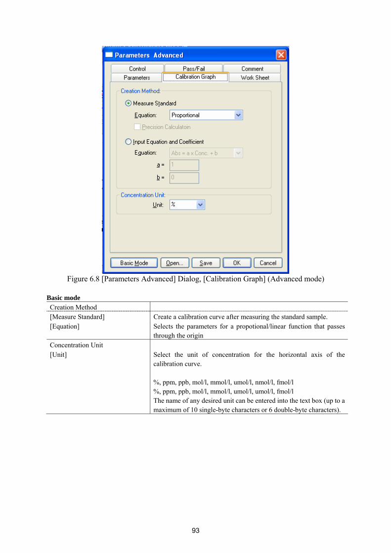
93

Figure 6.8 [Parameters Advanced] Dialog, [Calibration Graph] (Advanced mode)

Basic mode Creation Method [Measure Standard] Create a calibration curve after measuring the standard sample. [Equation] Selects the parameters for a propotional/linear function that passes

through the origin Concentration Unit [Unit] Select the unit of concentration for the horizontal axis of the

calibration curve. %, ppm, ppb, mol/l, mmol/l, umol/l, nmol/l, fmol/l %, ppm, ppb, mol/l, mmol/l, umol/l, umol/l, fmol/l The name of any desired unit can be entered into the text box (up to a maximum of 10 single-byte characters or 6 double-byte characters).

94

Advanced mode Creation method [Measure Standard] Select this option to create a calibration curve after measuring the

standard sample. [Equation] Select from the listed below.

Proportional : a straight line that passes through the origin Quadratic with Zero : quadratic function that passes through the originCubic with Zero : cubic function that passes through the origin Line Segment with Zero : polygonal function that passes

through the origin Linear : linear function Quadratic : quadratic function Cubic : cubic function Line Segment : polygonal function Spline : spline function Logistic : logistic function

[Precision Calculation] Available when a linear function/quadratic function/cubic function is selected for the function. When the [Precision Calculation] box is checked, the calibration graph displays a 95% confidence interval, and the limit of detection and the quantitative lower limit are displayed in the calibration information.

[Input Equation and Coefficient] Select this when creating a calibration curve by designating a function and coefficients.

[Equation] Select from the functions [Abs = aXConc+b] or [Conc = a x Abs+b] and enter the coefficients a and b.

Concentration Unit [Unit] Select the unit of concentration for the horizontal axis of the

calibration curve. %, ppm, ppb, mol/l, mmol/l, umol/l, umol/l and fmol/l Any desired unit can be entered into the text box (up to a maximum 10 single-byte characters or 6 double-byte characters).

95

The optimum calibration function can be selected from the modes shown in Fig.6.9, according to the application.

Segmented line Logistic function Spline function

Proportional expression Linear expression Quadratic expression Third-order expression

*Those modes marked with a “*” symbol can be selected to either pass through or not pass through the origin.

Figure 6.9 Calibration Curve Mode

If a calibration curve is created in advanced mode and a linear function, quadratic function or cubic function is selected as the calibration function, the calibration graph displays a 95% confidence interval and the limit of detection and the quantitative lower limit are displayed in the calibration information. The limit of detection, quantitative lower limit definitions, and calculation methods are as indicated below. Limit of Detection The limit of detection means the minimum concentrations at which the target substance and the blank can be differentiated. At JASCO, with the limit of detection is defined as “the minimum concentration at which it can be determined that the sample is not a blank with a 95% reliability”, the “concentration obtained from the calibration curve when an upper limit photometric value with a 95% confidence interval for a 0 concentration is taken” is calculated. Quantitative Lower Limit The quantitative lower limit is the minimum concentration that can be quantified with a given quantitative method. At JASCO, with the quantitative lower limit is defined as “the concentration at which the coefficient of variation of the concentration obtained using a calibration curve from a given photometric value is 10%” (see Fig. 6.10).

＊＊

＊

96

Figure 6.10 Limit of Detection and Quantitative Lower Limit

Concentration

Abs Abs

x Limit of Detection

x=Quantitative Lower Limit

Concentration

0.1x 11x

Calibration Curve 95% Confidence Interval

97

6.1.1.1.3 [Work Sheet] tab Worksheet settings can be configured in advanced mode. The data sheet used by the Calibration Curve Measurement program and the Quantitative Analysis program is created in the [Worksheet] tab. Widen the width of the [Parameters Advanced] dialog to display the entire worksheet window as shown in Figs. 6.11 and 6.12. Note: If an expression and coefficient are specified when creating a calibration curve, the

[Calibration Sheet] cannot be edited.

Figure 6.11 [Parameters Advanced] Dialog, [Work Sheet] tab (Calibration)

98

Figure 6.12 [Parameters Advanced] Dialog, [Work Sheet] tab (Quantitative)

<Add> Adds a row. <Insert> Inserts a row. <Delete> Deletes the currently selected row.

However, if the [Name] is displayed in blue, the row cannot be deleted.

99

[Calibration] button Click to set the calibration work sheet. [Quantitative] button Click to set the quantification work sheet.

[Name] Enter the column name. [Type] However, row types in which [Type] is displayed in red cannot be changed.

Selects the column type. Select from: character string, numeric values, date, and function

[Format] When inputting values such as photometric values, concentration, function, etc. into a column, click [Format] to select a display format. Selections: Standard, Integer,#.#, #.##, #.###, #.####, #.#####, Exponent

[Unit] Enter the unit when [Type] is set to a value or function. [Width] However, [Width] of row A in the [Calibration Sheet] cannot be changed

(Input Range: 0 to 100 mm). [Alignment] Sets alignment.

Selections: Left Side, Center, Right Side However, [Alignment] of row A on the [Calibration Sheet] cannot be changed.

[Equation] Input the numerical expression when [Type] is set as the function. Arithmetic operations that can be executed are +, –, × and ÷. Parentheses ( ) can also be used. Example of input: The following is an example displaying the dilution rate on row G and the concentration after correction using the dilution rate on row H of the quantification sheet. Set the [Type] for row G at values and that for row H at function, and enter D*G in the Equation column for row H.

Figure 6.13 Function Setup Example

100

6.1.1.1.4 [Control] tab

Figure 6.14 [Parameters Basic] Dialog, [Control] tab (Basic mode)

101

Figure 6.15 [Parameters Advanced] Dialog, [Control] tab (Advanced mode)

Basic mode Changeover wavelength [Light Source] Sets the changeover wavelength for the deuterium lamp and halogen lamp.

Enter a wavelength in the text box. Input range: 330 to 350 nm (default setting: 340 nm)

[Grating] Sets the photomultiplier and PbS changeover wavelength. Enter a wavelength in the text box. Input range: 750 to 900 nm (default setting: 800 nm) Note: The [Grating] changeover wavelength can only be set

for the V-670.

102

Advance mode Changeover wavelength [Light Source] Sets the changeover wavelength for the deuterium lamp and halogen lamp.


[Grating] Sets the photomultiplier and PbS changeover wavelength. Enter the wavelength in the text box. Input Range: 750 to 900 nm (default setting: 800 nm) Note: The [Grating] changeover wavelength can only be set

for the V-670.

Light Source [External Source] Select this when measuring with a light source other than the internal

deuterium lamp or halogen lamp. Correction [Dark Correction] Select when executing dark correction.

6.1.1.1.5 [Pass/Fail] tab

Figure 6.16 [Parameters Basic] Dialog, [Pass/Fail] tab

[Judgment] Select this when performing Pass/Fail judgment. Criteria Sets the criteria for the concentration of an unknown

103

sample. ≥ □and ≤ □ passes A photometric value of □ and above, □and below

passes. ≤ □ passes A photometric value of □ and below passes. ≥ □passes A photometric value of □and above passes. < □passes A photometric value of less than □passes. > □ passes A photometric value that is above □passes.

6.1.1.1.6 [Comment] tab

Figure 6.17 [Parameters Basic] Dialog, [Comment] tab

[Method] Input the quantitative method (maximum of 63 single-byte characters). [Description] Use as required (maximum of 63 single-byte characters). [Comment] For adding comments; use as required (maximum of 127 single-byte

characters). [User] Input the calibration curve user name. (maximum of 63 characters). [Division] Input the division of the calibration curve user (maximum of 127

characters).

104

6.1.1.2 [Open…] Opens a previously saved calibration file.

Note: This operation can also be performed with the tool button [Open].


[Look in] list Selects the drive or folder to browse using the drop-down menu.

Selects the filename to display from the filename list. [File name] Enter the filename. [Files of type] Sets the files to display in the filename list. Files other than the calibration

files (*uclb) cannot be selected. 6.1.1.3 [Save] The previously saved calibration curve is overwritten with the current filename. Executing this function overwrites any previous data saved under the same filename.

Note: This operation can also be performed with the tool button [Save].

105

6.1.1.4 [Save As…] Saves a newly created calibration curve under a new filename.


Figure 6.19 [Save data] Dialog

[Save In] list Select the drive and folder to save the file using the drop-down menu. File name list List of files that exist in the currently open folder. Refer to the list for file

naming. [File name] Enter the filename of the data for saving. If you have selected an existing

filename, the following dialog appears after clicking the <OK> button.

Figure 6.20 Dialog when an existing filename is designated Note: Clicking the <Yes> button will erase the original file.

[Save as type] Sets the files to display in the filename list. Files other than the calibration file (*uclb) cannot be selected.

106

6.1.1.5 [Export…] Saves the calibration curve in text format or CSV format. The filename, comment information, parameters, calibration curve information and calibration sheet are saved together.

Figure 6.21 [Export Data] Dialog

[Save in] list Selects the drive and folder to save the file using the drop-down menu. File name list List of files existing in the currently open folder. Refer to the list when

naming a file. To use an existing file, click on the desired filename. [File name] Enter the filename of the data to save. If you have selected an existing file

name, the following dialog appears after clicking the <OK> button.

Figure 6.22 Dialog when an existing filename is designated

Note: Clicking the <Yes> button will erase the original file.

[Save as type] list Sets the file to display in the filename list. Both the text format and CVS format can be selected.

107

6.1.1.6 [Open Template…] Selects a template file and opens its template.

Note: This operation can also be performed with the tool button [Open Template].


[Look in] list Select the drive or folder to browse using the drop-down menu. Filenames saved in the currently open folder are displayed in the filename list.

[File name] list Selects the filename of the template to be displayed. [File name] Enter the filename of the template to be displayed. The extension may be

omitted. The extension .uctp is automatically affixed. The filename can also be selected from the filename list.

[Files of type] Sets the files to display in the filename list. Files other than the template file (*uctp) cannot be selected.

<Open> Opens the template file. <Cancel> Closes the dialog without loading the template file.

108

6.1.1.7 [Save Template…] Enter a filename to save the currently opened template.

Note: This operation can also be performed with the tool button [Save Template].


[Save In] list Selects the drive or folder to browse using the drop-down menu. Filenames saved in the currently open folder are displayed in the filename list.

File name list Selects the filename of the template to save. [File name] Enter the filename of the template to save.

The extension may be omitted. The extension .uctp is automatically affixed.

[Save as type] Sets the files to display in the filename list. Files other than the template file (*uctp) cannot be selected.

<Save> Saves the template file and closes the dialog. <Cancel> Closes the dialog without loading the template file.

6.1.1.8 [Print…] The selected items set using the [Print Item] command are printed.

Note: This operation can also be performed with the tool button [Print].

109

6.1.1.9 [Print Preview…] Previews the print image.

Note: This operation can also be performed with the tool button [Print preview].


Button Name

[Print Item] Selects item to print.

[Margin] Sets margins.

[Font] Sets font of the title, information and data.

[Print] Starts printing.

110

6.1.1.10 [Print Item…] Selects item to print.

Figure 6.26 [Print Items] Dialog

[Title] Select when printing a title. [Calibration Curve Equation] Select when printing calibration curve information. [Comment] Select when printing comment information. [Measurement Information] Select when printing measurement information. Data Table [Auto Column Width] Automatically adjusts the data sheet column width to fit the text. [Column Wrap] If a data sheet does not fit on a single page, wraps the sheet's right edge and

prints. [Gridlines] Prints the data sheet with gridlines.

111

6.1.1.11 [Print Setup…] Sets the target printer and the printing conditions. The content of this dialog varies depending on the printer.


[Name] Displays the names of printers that can be used. To add a new printer, select

[Settings] - [Printer] from the Windows task bar and add the printer using [Add Printer].

[Paper] Selects the size and the method of feeding paper. [Orientation] Selects the paper orientation for printing.

6.1.1.12 [Exit] Exits the quantitative calibration program.

112

6.1.2 [Measure] Menu Starts and cancels the measurement and configures the calibration curve conditions. 6.1.2.1 [Cancel] Cancels the measurement.

Note: This operation can also be performed with the tool button [Cancel]. 6.1.2.2 [Sample] Used for starting measurement of a standard sample. Before starting measurement, confirm that the “*” mark is added on the row number of the data sheet to which information is to be entered. If it is not, click the row to measure. When the measurement is complete, the photometric values are displayed for each wavelength (peak, base 1, base 2) in the [Wavelength] column, and the vertical axis value of the calibration graph is displayed in the [Absorbance] column, and a checkmark “√” is automatically added to the [Use] field. It is also possible to enter the values directly into the [Concentration] and [Absorbance] columns of the worksheet to create the calibration line.

Note 1: The tool button [Sample] or the start button on the spectrophotometer can also be used.

Note 2: For repeat measurements, the value displayed in the [Wavelength] column is the average value of a number of measurements.

6.1.2.3 [Blank] Used for starting measurement of a blank sample. Confirm that there is nothing in the sample compartment or that the sample for the blank measurement is inserted and then press the <Measure> button. Once the measurement has been completed, the photometric values are displayed for each wavelength (peak, base 1, base 2) in the [Wavelength] column, and a checkmark “√” is automatically added to the [Use] field. Note 1: If a checkmark is added to the [Blank] row, [Use] checkbox of the worksheet, a value

with the blank value subtracted is displayed in the [Wavelength] column of the standard sample.

If blank correction is not necessary, uncheck the check box. Note 2: Regardless of the cursor location, when a [Blank] is performed, the results will always

be displayed in the blank measurement field of the first column, and the values of the standard sample in either the [Wavelength] column or the [Absorbance] column displayed in the data sheet are all corrected with the latest blank value.

Note 3: For repeat measurements, the displayed blank values is the average value of a number of measurements.

Note 4: This operation can also be performed with the tool button [Blank]. If the dialog shown in Fig. 6.27 is displayed, the blank measurement can be started using

the start button on the spectrophotometer.

113


<Measure> The blank measurement starts. <Cancel> The blank measurement is not performed and the [Blank Measurement]

dialog box closes. 6.1.2.4 [Dark] Available if [Dark] is selected in the [Parameters] - [Control] tab - [Correction] item in Advance mode. Block off the optical path of the sample side of the sample compartment with a shield and then press the <Measure> button. Note 1: If [Dark Correction] is selected when measuring a standard sample, the dark

correction cannot be cancelled later. Note 2: The dark measurement's photometric value is not displayed in the data sheet. The dark

correction uses the most recently measured dark value prior to the sample measurement. As a result, if a dark measurement is taken between sample measurements, the dark correction will have differing values before and after the dark measurement.

Note 3: In repeat measurements, a single measurement value is used as the dark value.

Note 4: This operation can also be performed with the tool button [Dark]. If the dialog shown in Fig. 6.29 is displayed, the blank measurement can be started using

the start button on the spectrophotometer.

Figure 6.29 [Dark Measurement] Dialog <Measure> The dark measurement starts <Cancel> The dark measurement is not performed and the [Dark Measurement]

dialog box closes.

114

6.1.2.5 [Parameters…] Changes the currently set calibration template settings. If the data sheet is empty, all items in the [Calibration Template] can be changed. If the data sheet is not empty, the content in [Creation Method] on the [Calibration Graph] tab, the [Quantitative Sheet] on the [Work Sheet] tab and the [Pass/Fail] and [Comment] tabs can be changed.

Note: This operation can also be performed with the tool button [Parameters]. 6.1.2.6 [Preview] [Preview] is a function that displays a general overview of the spectrum shape. Samples can be measured after performing baseline measurement using an air and a blank sample or they can be measured without performing baseline measurement The dialog box is composed of the spectrum display window and items (standard, control) for setting measurement parameters. These tabs can be changed over by clicking the tab for each item at the top of the dialog. Note 1: Baseline data and measurement results measured in [Preview] cannot be sent to

[Spectra Analysis] or be saved/printed. In addition, once the [Preview] dialog box is closed, the measurement parameters set using [Preview] cannot be used for normal measurements.

Note 2: This operation can also be performed with the tool button [Preview].

115

6.1.2.6.1 [Standard] tab

Figure 6.30 [Preview] Dialog

[Photometric Mode] Selectable range:

▪ Abs : Absorbance measurement ▪ %T : Transmittance measurement ▪ %R : Reflectance measurement

[Response] Response by simple moving average. The selectable range varies

depending on the model. V-630 : ▪ VQuick: Moving average over approx. 0.015 sec ▪ Quick: Moving average over approx. 0.06 sec ▪ Fast: Moving average over approx. 0.25 sec ▪ Medium: Moving average over approx. 1 sec ▪ Slow: Moving average over approx. 4 sec V-650/660/670 : ▪ Quick: Moving average over approx. 0.06 sec ▪ Fast: Moving average over approx. 0.25 sec ▪ Medium: Moving average over approx. 1 sec ▪ Slow: Moving average over approx. 4 sec

Note: The settings that can be made for scan speed vary

depending on the response (see Table 6.3).

[Bandwidth] Spectral bandwidth. The selectable range varies depending on the model.

116

V-630 : 1.5 nm (fixed) V-650/660 : 0.1, 0.2, 0.5, 1.0, 2.0, 5.0, 10, L2.0, L5.0, L10.0,

M1.0, M2.0 nm V-670 : 0.1, 0.2, 0.5, 1.0, 2.0, 5.0, 10, L2.0, L5.0, L10.0, M1.0, M2.0 nm (UV/Vis region) 0.4, 0.8, 2.0, 4.0, 8.0, 20.0, 40, L8.0, L20.0, L40.0, M4.0,

M8.0 nm (NIR region) Note 1: “L” is Low Stray Light Mode, “M” is Micro Cell Mode.

If a micro cell with an optical path width of 2 or 3 mm is used, use M1 nm (M4 nm in the NIR region). If a semi-micro cell with an optical path width of 4 mm or more is used, use M2 nm (M8 nm in the NIR region).

Note 2: If continuously measuring from the NIR to the visible region on the V-670, use the normal bandwidth combination given in Table 6.4. If the bandwidth is set to a similar value in the two regions, the measurement value noise in the NIR region will increase.

[Scan speed] V-630/650/660/670: 10, 20, 40, 100, 200, 400, 1000, 2000,

4000, 8000 nm/min Note: The data intervals that can be set vary depending on the

scanning speed (see Table 6.5).

[Start] The long end of the measurement wavelength range. Paired with the [End] (wavelength). The input range varies depending on the model. V-630 : 190.0 to 1100.0 nm V-650 : 190.0 to 900.0 nm V-660 : 187.0 to 900.0 nm V-670 : 190.0 to 2700.0 nm

[End] Short wavelength end of the measurement wavelength range. [Data Pitch] Data collecting wavelength interval. Selectable range varies depending on

the model. V-630 : 0.1, 0.2, 0.5, 1, 2, 5 nm V-650/660 : 0.025, 0.05, 0.1, 0.2, 0.5, 1, 2 , 5 nm V-670 : 0.025, 0.05, 0.1, 0.2, 0.5, 1, 2 , 5 nm (Measurements only for the UV/Vis range) 0.1, 0.2, 0.5, 1, 2 and 5 nm (measurements including NIR

range) Note: The measurement wavelength range is restricted by the

[Data Pitch] (see Table 6.6).

[Vertical axis] Sets the upper and lower limits for the vertical axis range to display in the window. Mark the [Auto] check box to set the full scale to about 1.2 times the maximum width of the spectrum based on the measured result. Input range -10 to 10 (Abs)

117

Sample Select when performing a sample measurement. Baseline Select when performing a baseline measurement.

If a baseline measurement is not taken, baseline correction is not performed on sample measurements. If a baseline measurement is taken, the baseline correction is performed automatically.

<Measure> Starts the sample or baseline measurement. <Close> Closes the [Preview] dialog. Note: [Scan Mode] is fixed at a continuous scan.

Table 6.3 [Scanning Speed] and [Response] Combination Response VQuick* Quick Fast Medium Slow

Scanning speed (nm/min)

10 OK OK OK OK OK 20 OK OK OK OK OK 40 OK OK OK OK OK 100 OK OK OK OK OK 200 OK OK OK OK OK 400 OK OK OK OK ×

1000 OK OK OK OK ×

2000 OK OK OK × ×

4000 OK OK OK × ×

8000 OK OK × × ×

*VQuick can only be set on the V-630

Table 6.4 Combination of Band Widths for UV/VIS Region and NIR Region UV/Vis bandwidth (nm) NIR bandwidth (nm)

0.1 0.2 0.5 1

2 (L10) 5 (L10)

10 (L10) M1 M2

0.4 0.8 2 4

8 (L8) 20 (L20) 40 (L40)

M4 M8

118

Table 6.5 Combination of [Scan] and [Data Pitch] Data pitch 0.025* 0.05* 0.1 0.2 0.5 1 2 5

Scanning speed 10 OK OK OK OK OK OK OK OK 20 OK OK OK OK OK OK OK OK 40 OK OK OK OK OK OK OK OK 100 × OK OK OK OK OK OK OK 200 × × OK OK OK OK OK OK 400 × × × OK OK OK OK OK

1000 × × × × OK OK OK OK 2000 × × × × × OK OK OK 4000 × × × × × × OK OK 8000 × × × × × × × OK

* On the V-630, there are no data pitches of 0.025, 0.05 nm.

Table 6.6 Combination of [Data interval] and [Wavelength range] Data interval Wavelength range

0.025* 750 0.05* 1500

0.1 and over Entire range can be measured. * On the V-630, there are no data pitches of 0.025nm, 0.05nm.

119

6.1.2.6.2 [Control] tab

Figure 6.31 [Preview] Dialog, [Control] tab

Changeover wavelength [Light Source] Sets the changeover wavelength for the deuterium lamp and halogen lamp.

Enter the wavelength in the text box. Input Range: 330 to 350 nm (Default Setting: 340 nm)

[Grating/Detector] Sets the photomultiplier and PbS changeover wavelength. Enter the wavelength in the text box. Input Range: 750 to 900 nm (Default Setting: 800 nm) Note: The [Detector/Grating] changeover wavelength can

only be set on the V-670.

[Filter Exchange] Sets whether to stop the scan and change filter or change the filter without stopping the scan. Note: If the filter is changed without stopping the scan, the

measurement time can be shortened, but noise may appear at the filter changeover wavelength as indicated in Fig. 6.32.

120

98

102

99

100

101

190 27001000 2000

%T

Wavelength [nm] Figure 6.32 (Top) Filter changeover without sopping the scan.

(Bottom) Scan is stopped and filter changed. 6.1.3 [Control] Menu 6.1.3.1 [Move Wavelength…] Moves the wavelength of the spectrophotometer to a desired wavelength.

Figure 6.33 [Move Wavelength] Dialog

[Move To] Text box for entering the wavelength.

The input range varies depending on the model. V-630 : 190.0 to 1100.0 nm V-650 : 190.0 to 900.0 nm V-660 : 187.0 to 900.0 nm V-670 : 190.0 to 2700.0 nm

<OK> Moves the wavelength of the spectrophotometer to the set wavelength. <Cancel> Closes the dialog without changing the previously set wavelength.

Note: This operation can also be performed with the tool button [Move Wavelength]. 6.1.3.2 [Optical Path] The [Optical Path] is a function for observing the optical path when changing the light source to the zero-order of the halogen lamp. When the [Optical Path] command is selected, the [Optical Path Check] dialog is displayed (see Fig. 6.34) and the switch to the zero-order halogen lamp is performed. Once the switch to zero-order is completed, Fig. 6.35 is displayed and the bandwidth can be changed to monitor the optical path. Click the <OK> button and Fig. 6.36 is displayed, and the status of the bandwidth and wavelength return to the state they were in before the [Optical Path Check] command was executed.

121

Figure 6.34 [Optical Path Check] Dialog 1



[Band Width] The selectable range varies depending on the model.

V-630 : 1.5 nm (fixed) V-650/660/670 : 0.1, 0.2, 0.5, 1.0, 2.0, 5.0, 10, L2.0, L5.0, L10.0, M1.0,

M2.0 nm <OK> The [Optical Path Check] dialog box closes and the bandwidth and

wavelength return to the state they were in before the [Optical Path Check] command was executed.

Note: This operation can also be performed with the tool button [Optical Path].

122

6.1.3.3 [Band Width] Changes the currently monitored bandwidth. When starting a measurement, the actual measurement starts once the bandwidth returns to the value set in [Parameters]. Note 1: The [Band Width] command is not displayed on the V-630. Note 2: On the V-670, the bandwidths that can be set vary depending on whether the current

wavelength is in the UV/VIS region or the NIR region.

Figure 6.37 [Band Width] Popup Menu

(UV/Vis region)

Figure 6.38 [Band Width] Popup Menu

(NIR region)

Note: This operation can also be performed with the tool button [Band width].

123

6.1.3.4 [Response] Changes the currently monitored response. When starting a measurement, the actual measurement starts once the response returns to the value set in [Parameters].

Figure 6.39 [Response] Popup Menu

Note 1: This operation can also be performed with the tool button [Response]. Note 2: The VQuick setting is also possible on the V-630 6.1.3.5 [Light Source] Displays the lamp use time and toggles the lamp on/off. When starting a measurement, the actual measurement starts once the lamp status returns to the status set in [Parameters].

Figure 6.40 [Light Source Control] Dialog

<OK> The settings are applied and the [Light Source Control] dialog box closes.<Cancel> The settings are deactivated and the [Light Source Control] dialog box

closes.

Note1: Turning the light ON/OFF can also be performed with the tool button

[Deuterium lump] and [Halogen lump]. Note 2: It takes approximately 5 minutes for the light source to stabilize. Refrain from taking a

measurement until the light source has stabilized.

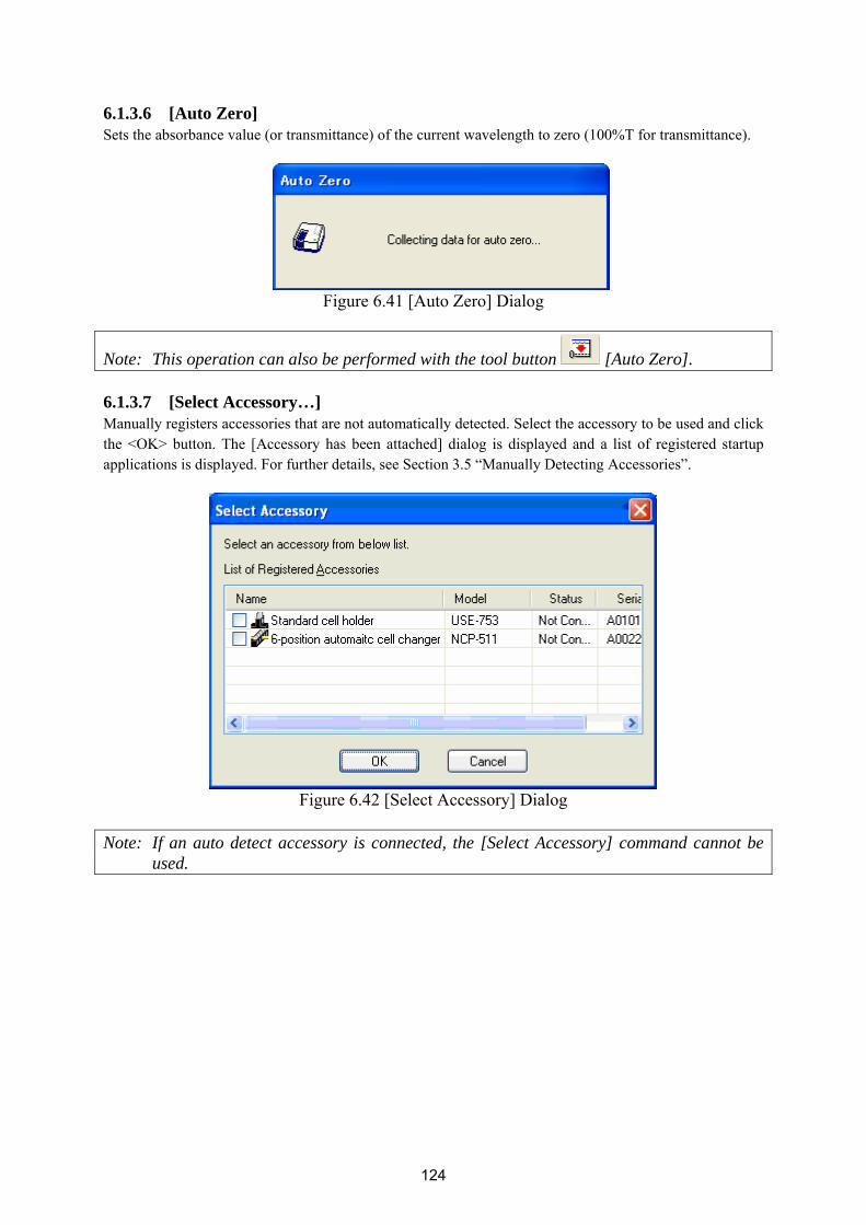
124

6.1.3.6 [Auto Zero] Sets the absorbance value (or transmittance) of the current wavelength to zero (100%T for transmittance).

Figure 6.41 [Auto Zero] Dialog

Note: This operation can also be performed with the tool button [Auto Zero]. 6.1.3.7 [Select Accessory…] Manually registers accessories that are not automatically detected. Select the accessory to be used and click the <OK> button. The [Accessory has been attached] dialog is displayed and a list of registered startup applications is displayed. For further details, see Section 3.5 “Manually Detecting Accessories”.


Note: If an auto detect accessory is connected, the [Select Accessory] command cannot be

used.

125

6.1.4 [Edit] Menu 6.1.4.1 [Copy Graph] Copies the calibration curve as a picture or a bitmap. 6.1.4.2 [Copy Table] Copies measurement conditions, comments, calibration curve information and data sheets. 6.1.4.3 [Delete] Click the number of the row to be deleted from the data sheet and select the [Delete] command. The following window is displayed. Clicking the <Yes> button deletes the selected row from the data sheet. Multiple contiguous lines can be selected and deleted.

Figure 6.43 [Delete Data] Dialog

6.1.4.4 [Delete All] Used to clear an entire data sheet. Select the [Delete All] command to display the following window. Clicking the <Yes> button deletes all data displayed in the sheet.

Figure 6.44 [Delete All Data] Dialog

126

6.1.5 [View] Menu Used for setting display. 6.1.5.1 [Decimal Point…] Sets the number of decimal places to display for the photometric value on the monitor bar.

Figure 6.45 [Decimal Point] Dialog

[Decimal Point] Sets the number of decimal places to display for the selected items in the

[Item] list. 6.1.5.2 [Information Bar] Sets whether to show/hide the information bar. 6.1.5.3 [Tool Bar] Sets whether to show/hide the tool bar. [File] Shows/hides the toolbar corresponding to the [File] menu. [Measure] Shows/hides the toolbar corresponding to the [Measure] menu. [Control] Shows/hides the toolbar corresponding to the [Control] menu. [View] Shows/hides the toolbar corresponding to the [View] menu.

6.1.5.4 [Status Bar] Sets whether to show/hide the status bar.

127

6.1.5.5 [Customize Toolbar…] Sets whether to show/hide and makes changes to the toolbar.

Figure 6.46 [Edit Toolbar] Dialog

[File] Shows/hides the toolbar corresponding to the [File] menu. Adds/deletes the

toolbar buttons to display.

Button Name

[New]

[Open]

[Save]

[Open Template]

[Save Template]

[Print]

[Print Preview]

[Measure] Shows/hides the toolbar corresponding to the [Measure] menu.

Adds/deletes the toolbar buttons to display.

Button Name

[Cancel]

[Sample]

[Blank]

[Dark]

[Parameters]

[Preview]

[Control] Shows/hides the toolbar corresponding to the [Control] menu. Adds/deletes

the toolbar buttons to display.

Button Name

[Move Wavelength]

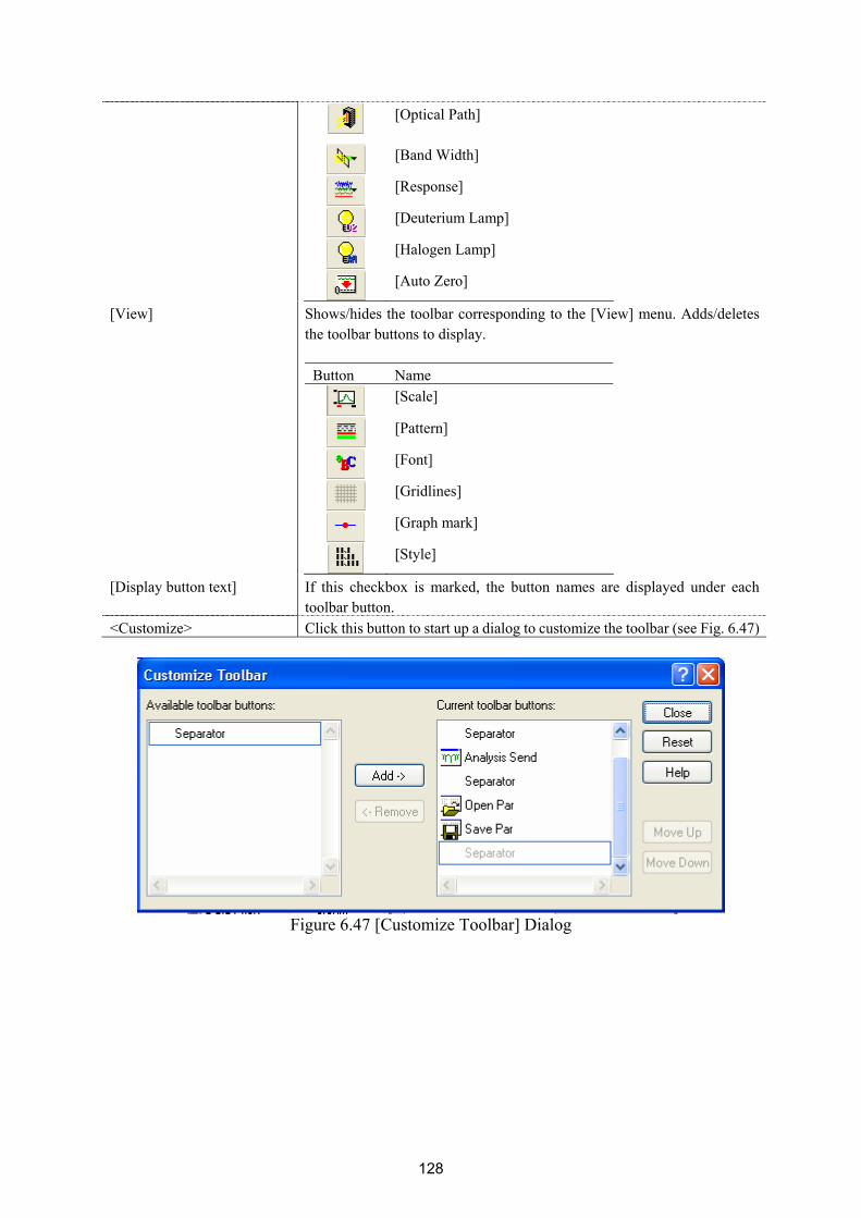
128

[Optical Path]

[Band Width]

[Response]

[Deuterium Lamp]

[Halogen Lamp]

[Auto Zero]

[View] Shows/hides the toolbar corresponding to the [View] menu. Adds/deletes


Button Name

[Scale]

[Pattern]

[Font]

[Gridlines]

[Graph mark]

[Style]

[Display button text] If this checkbox is marked, the button names are displayed under each

toolbar button. <Customize> Click this button to start up a dialog to customize the toolbar (see Fig. 6.47)

Figure 6.47 [Customize Toolbar] Dialog

129

6.1.5.6 [Calibration Graph] Sets the calibration graph display form. 6.1.5.6.1 [Scale] Changes the display scale of the calibration graph.

Figure 6.48 [Scale] Dialog

[Vertical Axis] Enters the scale of the horizontal axis. Checking the [Auto] check box

displays the entire range ignoring the input values. [Horizontal Axis] Enters the scale of the vertical axis. Checking the [Auto] check box

displays the graph with the optimum scale for the designated horizontal axis range.

Note: This operation can also be performed with the tool button [Scale]. 6.1.5.6.2 [Pattern] Sets the display color and line style of the calibration graph.

Figure 6.49 [Pattern Settings] Dialog

130

[Element] list Select an element to change colors and line styles of the calibration curve,

frame, grid line and auxiliary grid line. [Color] Changes the color of the element selected in the [Element] list. [Line Style] Sets the line format of the element selected from the [Element] list. [Line Width] Sets the line width. [Sample] Displays a sample of the designated style. [Set As Default] Check this check box to apply the subsequent display.

Note: This operation can also be performed with the tool button [Pattern]. 6.1.5.6.3 [Font] Designates the display font.

Figure 6.50 [Font] Dialog

[Item] list Select items to set the font for.

[Axis Label]: Character ([Abs], [nm] or other) [Scale Label]: Numeric value

[Vertical Label Orientation] Select the orientation in which the axis label is to be displayed. [Horizontal]: Horizontal to the calibration graph display window [Vertical]: Vertical to the calibration graph display window

[Set As Default] Check this check box to apply to the subsequent display.

<Setting…> Opens the [Font] dialog.

<Close> Closes the dialog after applying settings to items.

<Cancel> Closes the dialog without applying settings to items.

131


[Font] Selects a font. [Font style] Selects a font style. [Size] Selects a font size. [Effects] Strikeout and underline can be specified. [Color] list Selects the font color. [Sample] Displays a sample of the specified font. [Script] Selects the language for the specified font. <OK> Sets the font and returns to the [Font] dialog. <Cancel> Returns to the [Font] dialog without applying font settings.

Note: This operation can also be performed with the tool button [Font]. 6.1.5.6.4 [Gridlines…] Sets whether to show/hide grid lines.

Figure 6.52 [Grid Lines] Dialog

132

[Main: Horizontal Axis] Check this check box to display main grid lines for the horizontal axis. [Main: Vertical Axis] Check this check box to display main grid lines for the vertical axis. [Auxiliary: Horizontal Axis] Check this check box to display auxiliary grid lines for the horizontal axis.[Auxiliary: Vertical Axis] Check this check box to display auxiliary grid lines for the vertical axis. [Set As Default] Check this check box to apply the subsequent display.

Note: This operation can also be performed with the tool button [Gridlines]. 6.1.5.6.5 [Marker Settings] Sets the type, size and color of the marker that displays the calibration curve data points and sets whether to fill the marker.

Figure 6.53 [Marker Settings] Dialog

[Type] Type of the marker of the calibration curve. Select from circle, square,

triangle, diamond, cross and star. [Size] Size of the marker [Color] List of color samples. Select one from the list. [Fill inside] Check box to set filling/non-filling the marker. Check the check box to fill

the marker. [Sample] Displays a sample of the designated marker. [Set As Default] Check this check box to apply the subsequent display.

Note: This operation can also be performed with the tool button [Marker setting].

133

6.1.5.6.6 [Style…] Sets the calibration curve graph display style.


[Axis] Select the setting form of the vertical or horizontal axis. [Scale label] [Interval: Auto] Check this check box to set the scale display method “Auto”. [Interval: Manual] Check this check box to set the scale display to the desired interval. In

manually setting, the intervals of the main and auxiliary scale labels can also be set.

[Decimal Point on Scale Label]

Sets the number of decimal places for the vertical and horizontal display values.

[Set As Default] Check this check box to apply the subsequent display.

Note: This operation can also be performed with the tool button [Style].

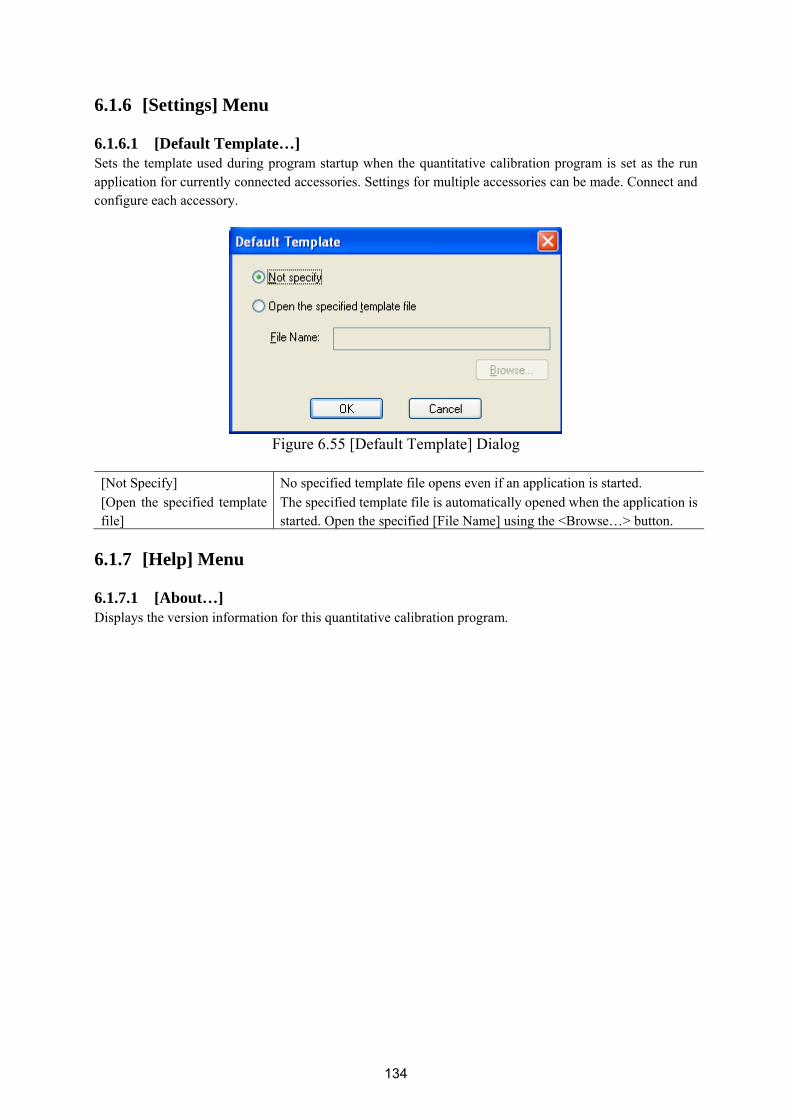
134

6.1.6 [Settings] Menu 6.1.6.1 [Default Template…] Sets the template used during program startup when the quantitative calibration program is set as the run application for currently connected accessories. Settings for multiple accessories can be made. Connect and configure each accessory.

Figure 6.55 [Default Template] Dialog

[Not Specify] No specified template file opens even if an application is started. [Open the specified template file]

The specified template file is automatically opened when the application is started. Open the specified [File Name] using the <Browse…> button.

6.1.7 [Help] Menu 6.1.7.1 [About…] Displays the version information for this quantitative calibration program.

135

6.2 [Quantitative Measurement] Program Reference The [Quantitative Measurement] program is used to make quantitative measurements. Open a calibration file created with the [Quantitative Calibration] program to not only make quantitative measurements, but also to open a template file to do everything from creating a calibration curve to making quantitative measurements.


Information bar Displays measurement parameters and accessory information.

Calibration/Quantitative view field Shows the calibration and quantitative sheets set with the [Quantitative Calibration] program (advanced mode).

Monitor bar Shows the current wavelength, photometric value and number of cycles. Toolbar

Performs measurement and adjusts parameter settings using the buttons on this toolbar (refer to Table 6.7 for details). The tool button can be customized in the [View] menu.

Deuterium lamp/Halogen lamp Displays the lamp status. Lamp cannot be turned On/Off using this icon.

Calibration graph/Calibration curve information display field Displays the calibration curve graph and calibration curve information. The display style is set in the [View] menu.

136

Table 6.7 Tool Bar Icons and Names Button Name Reference Section

[New] 6.2.1.1 [New…]

[Open] 6.2.1.2 [Open…]

[Save] 6.2.1.3 [Save…]

6.2.1.4 [Save As…]

[Print] 6.2.1.6 [Print…]

[Print Preview] 6.2.1.7 [Print Preview…]

[Cancel] 6.2.2.1 [Cancel]

[Sample] 6.2.2.2 [Sample]

[Blank] 6.2.2.3 [Blank]

[Dark] 6.2.2.4 [Dark]

[Parameters] 6.2.2.5 [Parameters…]

[Exit Modification] 6.2.2.6 [Exit Modification]

[Move wavelength] 6.2.3.1 [Move wavelength]

[Optical Path] 6.2.3.2 [Optical Path…]

[Deuterium Lamp]

Note: Displays the deuterium lamp status. Lamp

cannot be turned On/Off using this icon.

[Halogen Lamp]

Note: Displays the halogen lamp status. Lamp cannot be turned On/Off using this icon.

[Auto Zero] 6.2.3.3 [Auto Zero]

[Scale] 6.2.5.6.1 [Scale…]

[Pattern] 6.2.5.6.2 [Pattern…]

[Font] 6.2.5.6.3 [Font…]

[Gridlines] 6.2.5.6.4 [Gridlines…]

[Marker Settings] 6.1.5.6.5 [Marker Settings…]

[Style] 6.1.5.6.6 [Style…]

137

Window Title bar Displays the name of the program window. Menu bar Displays the menus that can be used. Monitor bar Wavelength, photometric value and current cycle number are displayed

from left to right Information bar Displays the current measurement parameters/accessory information. [Calibration curve graph] window

Displays the calibration curve graph.

[Calibration curve information] window

Displays calibration curve information.

[Calibration curve sheet] window

Shows the quantitative sheet format set with the [Quantitative Calibration] program (advanced mode).

[Quantification sheet] window

Shows the quantitative sheet format set with the [Quantitative Calibration] program (advanced mode).

Status bar Displays information about the instrument status and explanations of selected menus.

Menu [File] menu [New …] Starts a new quantitative measurement from a template or calibration file.[Open …] Opens a previously saved quantification result file. [Save …] Saves the quantification result under an existing filename. [Save As …] Saves the quantification result under a new filename. [Export …] The quantitative results are saved as a text file or in the CSV format. [Print …] Prints out the quantification result. [Print Preview …] Gives a preview of the image to be printed. [Print Item…] Sets the print items. [Print Setup …] Sets the printer and print parameters. [Exit] Exits the quantitation analysis program and returns to [Spectra Manager].[Measure] menu [Cancel] Cancels measurement. [Sample] Starts sample measurement. [Blank] Measures data for baseline correction. [Dark] Measures data for dark correction. [Parameters …] Sets the parameters, saves and loads the parameters. [Exit Modification] Exits calibration curve editing, changes to quantitative mode. [Control] menu [Move Wavelength …] Moves the wavelength of the spectrophotometer to the desired wavelength.[Optical Path…] Changes to zero-order light source for checking the optical path. [Auto Zero …] Sets the absorbance value (or transmittance) of the current wavelength to

zero (100%T for transmittance). [Select Accessory...] Selects an accessory. [Edit] menu [Copy Graph] Copies the calibration curve as a picture or bitmap.

[Copy Table] Copies measurement conditions, comments, calibration curve information and data sheets.

[Delete] Deletes selected lines.

138

[Delete All] Deletes all the displayed data. [Edit Comment...] Edits comment information. [View] menu [Decimal Point...] Sets the number of decimal points to display for the photometric value on

the monitor bar. [Information Bar …] Sets whether to show/hide the information bar. [Toolbar] Sets whether to show/hide the toolbar. [Status bar] Sets whether to show/hide the status bar. [Customize Toolbar...] Changes and sets the toolbar. [Calibration Graph] [Scale …] Sets the scales of the vertical and horizontal axes of the calibration graph.[Pattern …] Sets the color, line style and line width of the calibration curve, frame and

grid lines. [Font …] Sets the font of the calibration graph. [Gridlines …] Sets whether to show/hide the gridlines for the vertical and horizontal axes

of the calibration curve graph. [Graph Mark …] Sets the format, size and color of the data points for the calibration curve,

and the color and filling/non-filling of the markers. [Style…] Sets the calibration curve graph display style. [Setting] Menu [Default Parameters...] When a currently recognized accessory is connected, this sets the

calibration curve template or calibration file to open when the application starts up.

[Help] menu [About …] Displays the version information for the program.

139

6.2.1 [File] Menu Used to save or print measurement results. 6.2.1.1 [New…] This menu item closes the currently opened calibration curve and quantitative results and begins a new measurement.


[Create using Template] Select this option when performing quantitative measurement using an

existing template file and creating a new calibration curve. [Create using Calibration File] Select this option when performing quantitative measurement using an

existing calibration curve.

Note: This operation can also be performed with the tool button [New]. When [Create using Calibration File] is selected. Opens the template file created with the [Quantitative Calibration] program, and once the calibration curve has been created, executes a quantitative measurement.


140

When [Create using Calibration File] is selected. Opens calibration files created with the [Quantitative Calibration] program and starts quantitative measurement.


6.2.1.2 [Open …] Opens a saved quantification result file.



[Look in] list Select the drive or folder to browse using the drop-down menu.

Select the file name to display from the filename list. [File name] Enter the filename. [Files of type] list Sets the files to display in the filename list. Files other than the

quantification result file (*uqnd) cannot be selected.

141

6.2.1.3 [Save] Executing this function overwrites any previous data saved under the same filename.

Note: This operation can also be performed with the tool button [Save]. 6.2.1.4 [Save As …] Saves the quantification result under a new filename.



[Save in] list Selects the drive or folder for saving using the drop-down menu. File name list List of files in the currently open folder. Refer to it when assigning a name

to a file. [File name] Enter the filename of the data for saving. If an existing filename is selected,

the following dialog appears after clicking the <OK> button.

Figure 6.62 Dialog when an existing filename is designated Note: Clicking the <Yes > button will erase the original file.

[Save as type] Sets the files to display in the filename list. Files other than quantification result files (*uqnd) cannot be selected.

142

6.2.1.5 [Export…] Saves quantitative measurement results in text format or in CSV format. The filename, comment information, measurement parameters, calibration curve data, and calibration and quantitative sheets are saved. Note: If the quantitative sheet is empty, [Export] cannot be used. To retain calibration curve

information prior to the quantitative measurement, select [Calibration Sheet] from the worksheet display and then select [Copy].

Figure 6.63 [Export Data] Dialog [Save in] list Selects the drive and folder to save the file using the drop-down menu. File name list List of files in the currently open folder. Refer to the list when naming a

file. [File name] Enter the filename of the data to save. If you have selected an existing


Figure 6.64 Dialog when existing filename is designated Note: Clicking the <Yes> button will erase the original file.

[Save as type] list Sets the files to display in the filename list. Both text format and CSV format can be selected.

143

6.2.1.6 [Print…] The selected item set using the [Print Item] command are printed.

Note: This operation can also be performed with the tool button [Print]. 6.2.1.7 [Print Preview…] Previews the print image.


Figure 6.65 Print Preview

Button Name



[Font] Sets font for the title, information and data.


144

6.2.1.8 [Print Item…] Selects items to print.


[Title] Select when printing a title. [Graph] Select when printing filename, comment information, measurement

conditions, calibration curve data and calibration sheets. [Comment] Select when printing comment information. [Measurement Information] Select when printing measurement information. Data Table [Auto Column Width] Automatically adjusts the data sheet column width to fit the text. [Column Wrap] If a data sheet does not fit on a single page, wraps the sheet's right edge and


145

6.2.1.9 [Print Setup…] Sets the target printer and the printing conditions. The content of this dialog varies depending on the printer.

Figure 6.67 [Print Setup] Window


[Settings] - [Printer] from the Windows task bar and add the printer using [Add Printer].

[Size] Selects the size and the method of feeding paper. [Orientation] Selects the paper orientation for printing.

6.2.1.10 [Exit] Exits the quantitative analysis program.

146

6.2.2 [Measure] Menu Starts and cancels the measurement and configures the calibration curve conditions. 6.2.2.1 [Cancel] Cancels the measurement.

Note: This operation can also be performed with the tool button [Cancel]. 6.2.2.2 [Sample] Used for starting measurement of a standard sample and sample of unknown concentration.


Note 2: For repeat measurements, the value displayed in the [Wavelength] column is the average value of a number of measurements. During quantitative measurements, the photometric value of the set number of times and its average are displayed in the [Wavelength] column.

Measuring a standard sample on the calibration sheet Used for starting measurement of a standard sample. Before starting a measurement, confirm that the “*” mark is added on the row number of the data sheet to which information is to be entered. If it is not, click the row to measure. When the measurement is complete, the photometric values are displayed for each wavelength (peak, base 1, base 2) in the [Wavelength] column, and the vertical axis value of the calibration graph is displayed in the [Absorbance] column, and a checkmark “√” is automatically added to the [Use] field. It is also possible to enter the values directly into the [Concentration] and [Absorbance] columns of the work sheet to create the calibration line. Measuring an sample of unknown concentration using the Quantitative sheet Used for starting measurement of sample of unknown concentration. When the measurement is complete, the photometric values are displayed for each wavelength (peak, base 1, base 2) in the [Wavelength] column and a value corresponding to the vertical axis of the calibration graph is displayed in the [Absorbance] column. The measurement value is always entered in a new row.

147

6.2.2.3 [Blank] Used for starting measurement of standard blank and sample blank. Note 1: For repeat measurements, the mean of the number of measurements is displayed in the

[Wavelength] column. During quantitative measurements, the photometric value of the set number of times and its average are displayed in the [Wavelength] column.

Note 2: This operation can also be performed with the tool button [Blank]. If the dialog shown in Fig. 6.68 is displayed, the blank measurement can be started using the start button on the spectrophotometer.


<Measure> The blank measurement commences. <Cancel> The blank measurement is not performed and the [Blank Measurement]

dialog box closes. When measuring a standard blank on the calibration sheet Confirm that there is nothing in the sample compartment or that the sample for the standard blank measurement is inserted and then press the <Measure> button. Once the measurement has been completed, photometric values are displayed for each wavelength (peak, base 1, base 2) in the [Wavelength] column and a checkmark “√” is automatically added to the [Use] field. Note 1: If a checkmark is added to the [Blank] row, [Use] checkbox of the worksheet, a value

with the blank value subtracted is displayed in the [Wavelength] column of the standard sample. If a blank correction is not necessary, uncheck the check box.

Note 2: Regardless of the cursor location, when a [Blank] is performed, the results will always be displayed in the blank measurement field of the first column, and the values of the standard sample in either the [Wavelength] column or the [Absorbance] column displayed in the data sheet are all corrected with the latest blank value.

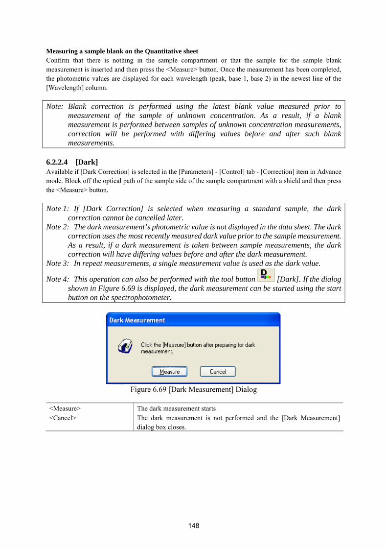
148

Measuring a sample blank on the Quantitative sheet Confirm that there is nothing in the sample compartment or that the sample for the sample blank measurement is inserted and then press the <Measure> button. Once the measurement has been completed, the photometric values are displayed for each wavelength (peak, base 1, base 2) in the newest line of the [Wavelength] column. Note: Blank correction is performed using the latest blank value measured prior to

measurement of the sample of unknown concentration. As a result, if a blank measurement is performed between samples of unknown concentration measurements, correction will be performed with differing values before and after such blank measurements.

6.2.2.4 [Dark] Available if [Dark Correction] is selected in the [Parameters] - [Control] tab - [Correction] item in Advance mode. Block off the optical path of the sample side of the sample compartment with a shield and then press the <Measure> button. Note 1: If [Dark Correction] is selected when measuring a standard sample, the dark

correction cannot be cancelled later. Note 2: The dark measurement’s photometric value is not displayed in the data sheet. The dark


Note 3: In repeat measurements, a single measurement value is used as the dark value.

Note 4: This operation can also be performed with the tool button [Dark]. If the dialog shown in Figure 6.69 is displayed, the dark measurement can be started using the start button on the spectrophotometer.

Figure 6.69 [Dark Measurement] Dialog

<Measure> The dark measurement starts <Cancel> The dark measurement is not performed and the [Dark Measurement]

dialog box closes.

149

6.2.2.5 [Parameters…] Changes the calibration conditions of the currently set calibration graph. It can be used when creating a calibration curve with the quantitative measurement program. The items that can be changed are [Calibration Graph], [Quantitative Sheet] on the [Worksheet], [Pass/Fail], and [Comment]. Once editing of the calibration curve has been completed and the program changed to quantitative mode, the calibration conditions cannot be changed.

Note: This operation can also be performed with the tool button [Parameters]. 6.2.2.6 [Exit Modification] Used when a calibration curve has been created by this program, and for switching to quantitative mode after completing calibration curve creation. When the <Yes> button in Figure 6.70 is clicked, calibration curve modification mode is exited and the mode changes to quantitative mode.

Figure 6.70 [Finish the modification of calibration] Dialog

Note 1: Once the mode has been changed to quantitative mode, the calibration curve can no

longer be edited.

Note 2: This operation can also be performed with the tool button [Exit Modification]. 6.2.3 [Control] Menu 6.2.3.1 [Move Wavelength…] Moves the wavelength of the spectrophotometer to the desired wavelength.


[Move To] Text box to enter the wavelength.


150


Note: This operation can also be performed with the tool button [Move Wavelength]. 6.2.3.2 [Optical Path] The [Optical Path] is a function for observing the optical path when changing the light source to the zero-order of the halogen lamp. When the [Optical Path] command is selected, the [Optical Path Check] dialog is displayed (see Fig. 6.72) and the switched to the zero-order halogen lamp is performed. Once the switch to the zero-order is completed, Fig. 6.73 is displayed and the bandwidth can be changed to monitor the optical path. Click the <OK> button and Fig. 6.74 is displayed, and the status of the bandwidth and wavelength return to the state they were in before the [Optical Path Check] command was executed.




[Band Width] Sets the bandwidth.

The selectable range varies depending on the model. V-630 : 1.5 nm (fixed) V-650/660/670 : 0.1, 0.2, 0.5, 1.0, 2.0, 5.0, 10, L2.0, L5.0, L10.0, M1.0,

151

M2.0 nm <OK> The [Optical Path Check] dialog box closes and the bandwidth and

wavelength return to the state they were in before the [Optical Path Check]

command was executed.

Note: This operation can also be performed with the tool button [Optical Path Check]. 6.2.3.3 [Auto Zero] Sets the absorbance value (or transmittance) of the current wavelength to zero (100%T for transmittance).


Note: This operation can also be performed with the tool button [Auto Zero]. 6.2.3.4 [Select Accessory …] Manually registers accessories that are not automatically detected. Select the accessory to be used and click the <OK> button. The [Accessory has been attached] dialog is displayed and a list of registered startup applications is displayed. For future details, see Section 3.5 “Manually Detecting Accessories”.


Note: If an auto detect accessory is connected, the [Select Accessory] command cannot be

used.

152

6.2.4 [Edit] Menu 6.2.4.1 [Copy Graph] Copies the calibration curve as a picture or a bitmap. 6.2.4.2 [Copy Table] If the calibration sheet is selected in the worksheet display field and [Copy] is selected, the filename, measurement conditions, comment information, calibration data and the calibration sheet are copied. If the quantitative sheet is selected and [Copy Table] is chosen, the filename, measurement conditions, comment information, calibration data and the quantitative sheet are copied. 6.2.4.3 [Delete] Click the number of the line to be deleted from the data sheet and select the [Delete] command. The following window is displayed. Clicking the <Yes> button deletes the selected line from the data sheet. Multiple contiguous lines can be selected and deleted.


Note: Blank data being used to correct samples of unknown concentrations cannot be deleted.


6.2.4.4 [Delete All] Used to clear an entire data sheet. Select the [Delete All] command to display the following window. Clicking the <Yes> button deletes all the data displayed in the sheet.


153

6.2.4.5 [Comment…] Edits the comment information.

Figure 6.80 [Edit Information] Dialog

[Name] For assigning a name to the data (maximum of 63 single-byte characters). [Comment] For adding comments; use as required (maximum of 127 single-byte

characters). [User] Input the name of the user performing the quantitative measurement

(maximum of 63 single-byte characters). [Division] Input the division of the user making the quantitative measurement; use as

required (maximum of 127 characters). [Company] The company is automatically entered (maximum of 63 characters).

6.2.5 [View] Menu Used for setting display. 6.2.5.1 [Decimal Point…] Sets the number of decimal places to display for the photometric value on the monitor bar.


[Decimal Point] Sets the number of decimal places to display for the selected items in the

[Item] list.

154

6.2.5.2 [Information bar] Sets whether to show/hide the information bar. 6.2.5.3 [Tool bar] Sets whether to show/hide the tool bar. [File] Shows/hides the toolbar corresponding to the [File] menu. [Measure] Shows/hides the toolbar corresponding to the [Measure] menu. [Control] Shows/hides the toolbar corresponding to the [Control] menu. [View] Shows/hides the toolbar corresponding to the [View] menu.

6.2.5.4 [Status bar] Sets whether to show/hide the status bar. 6.2.5.5 [Customize Toolbar…] Sets whether to show/hide and makes changes to the toolbar.




Button Name

[New]

[Open]

[Save]

[Print]

[Print Preview]

[Measure] Shows/hides the toolbar corresponding to the [Measure] menu..


Button Name

[Cancel]

[Sample]

155

[Blank]

[Dark]

[Parameters]

[Exit Modification]



Button Name

[Move Wavelength]

[Optical Path]

[Deuterium Lamp]

[Halogen Lamp]

[Auto Zero]



Button Name

[Scale]

[Pattern]

[Font]

[Gridlines]

[Marker Settings]

[Style]

[View Name] If this checkbox is checked, the button names are displayed under each tool

button. <Customize> Click this button to start up a dialog to customize the toolbar (see Fig. 6.83)


156

6.2.5.6 [Calibration Graph] Sets the calibration graph display form. 6.2.5.6.1 [Scale] Changes the display scale of the calibration graph.


Horizontal Axis Scale Enters the scale of the horizontal axis. Checking the [Auto] check box

displays the entire range ignoring the input values.

Vertical Scale Enter the scale of the vertical axis. Checking the [Auto] check box

displays the graph with the optimum scale for the designated horizontal

axis range.

Note: This operation can also be performed with the tool button [Scale].

157

6.2.5.6.2 [Pattern] Sets the display color and line style of the calibration graph.


[Element] list Select an element to change colors and line styles of the calibration curve,

frames, grid lines and auxiliary grid lines. [Color] Changes the color of the element selected in the [Element] list. [Line Style] Sets the line format of the element selected from the [Element] list. [Line Width] Sets the line width. [Sample] Displays a sample of the designated style. [Set As Default] Check this check box to apply in the subsequent display.

Note: This operation can also be performed with the tool button [Pattern]. 6.2.5.6.3 [Font] Designates the display font.

Figure 6.86 [Font] dialog

158

[Item] Selects items to set the font for.

[Axis Label]: Character ([Abs], [Concentration] or other) [Scale Label]: Numeric value

[Vertical Label Orientation] Selects the orientation in which the axis label is to be displayed. [Horizontal]: Horizontal to the calibration graph display window [Vertical]: Vertical to the calibration graph display window

[Set As Default]

If [Set As Default] is checked, the specified font will be applied to the following [Calibration Graph] window.

<Setting...> Opens the [Font] dialog. <Close> Closes the dialog after applying settings to items.


Figure 6.87 [Font] dialog

[Font] Selects a font. [Font Style] Selects a font style. [Size] Selects a font size. [Effects] Strikeout and underline can be specified. [Color] list Selects the font color. [Sample] Displays a sample of the specified font. [Script] Selects the language for the specified font. ＜OK＞ Sets the font and returns to the [Font] dialog. <Cancel> Returns to the [Font] dialog without applying font settings.

Note: This operation can also be performed with the tool button [Font].

159

6.2.5.6.4 [Gridlines…] Sets whether to show/hide grid lines.



Note: This operation can also be performed with the tool button [Gridlines]. 6.2.5.6.5 [Market settings…] Sets the type, size and color of the marker that displays the calibration curve data points and sets whether to fill the marker.

Figure 6.89 [Marker Settings] Dialog

160

[Type] Type of the marker of the calibration curve. Select from circle, square,

triangle, diamond, cross and star. [Size] Size of the marker [Color] List of color samples. Select one from the list. [Fill Inside] Check box to set filling/non-filling the marker. Check the check box to fill

the marker. [Sample] Displays a sample of the designated marker. [Set As Default] Check this check box to apply the subsequent display.

Note: This operation can also be performed with the tool button [Marker setting]. 6.2.5.6.6 [Style] Sets the calibration curve graph display style.


[Axis] Select the setting form of the vertical or horizontal axis. [Scale label] [Interval: Auto] Check this check box to set the scale display method “Auto”. [Interval: Manual] Check this check box to set the scale display to the desired interval. In


[Decimal Point on Scale Label]




161

6.2.6 [Settings] Menu 6.2.6.1 [Default Parameters…] Sets the template used during program startup when the quantitative measurement program is set as the run application for currently connected accessories. Settings for multiple accessories can be made. Connect and configure each accessory.

Figure 6.91 [Default Parameter] Dialog

[Not Specify] No specified template file opens even if an application is started. [Open the specified template file]

The specified template file is automatically opened when the application is started. Open the specified [File Name] using the <Browse…> button.

[Open the Specified Calibration File]

The specified calibration file is automatically opened when the application is started. Open the specified [File Name] using the <Browse…> button.

6.2.7 [Help] Menu 6.2.7.1 [About…] Displays the version information for this quantitative calibration program.

162

7 [Spectra Measurement] Program Reference The Spectra Measurement program measures sample absorbance, transmittance and reflectivity spectra. When the Spectrum Measurement program is started, the following window is displayed.

Figure 7.1 [Spectra Measurement] window

Information bar Displays the current measurement parameters and accessory information.

Toolbar Common functions for measurement, parameter settings and others can be accessed with the buttons on this toolbar (see Table 7.1). The tool buttons can be customized in the [View] menu.

Monitor bar Displays the current wavelength, photometric value, number of cycles and number of accumulations.

Spectrum display Field Displays the spectrum being measured. The display format can be set using the [View] menu.

163


[Save Data] 7.1.1 [Save Data…]

[Analysis Send] 7.1.2 [Analysis Send]

[Open Parameters] 7.1.3 [Open Parameters…]

[Save Parameters] 7.1.4 [Save Parameters…]

[Cancel] 7.2.1 [Cancel]

[Sample] 7.2.2 [Sample]

[Baseline] 7.2.3 [Baseline]

[Dark] 7.2.4 [Dark]

[Parameters] 7.2.5 [Parameters…]

[Preview] 7.2.6 [Preview…]

[Move Wavelength] 7.3.1 [Move Wavelength…]

[Optical Path] 7.3.2 [Optical Path…]

[Band width] 7.3.3 [Band width…]

[Response] 7.3.4 [Response]

[Toggle Deuterium lamp] 7.3.5 [Light Source]

[Toggle Halogen lamp] 7.3.5 [Light Source]

[Auto Zero] 7.3.6 [Auto Zero]

[Scale] 7.4.1 [Scale…]

[Pattern] 7.4.2 [Pattern…]

[Font] 7.4.3 [Font…]

[Gridlines] 7.4.4 [Gridlines…]

[Style] 7.4.5 [Style…]

[Decimal Point] 7.4.7 [Decimal Point…]

164

Window Title bar Displays the name of the program window. Menu bar Displays the names of the menus that can be used. Monitor bar Displays the wavelength, photometric value, current cycle number

and number of accumulations from left to right. Tool bar Displays icons of available tools. The Tool buttons can be

customized in the [View] menu. Information bar Displays the current parameters, baseline/dark spectrum

information and accessory information. Spectrum display field Monitors spectra during measurement Status bar Displays information about the instrument status and explanations

of selected menus. Menu [File] menu [Save Data] Saves spectrum under a new filename. [Analysis Send] Transfers the measurement result to the Spectra Analysis program[Open Parameters…] Selects a parameter file and opens those parameters. [Save Parameters…] Saves parameters using entered filename. [Open Baseline…] Opens a saved baseline to be used for measurement. [Save Baseline…] Assigns a filename and saves the baseline currently being used. [Open Dark…] Opens a saved dark spectrum to use for measurement. [Save Dark…] Assigns a filename and saves the dark spectrum currently being

used. [Exit] Exits the spectra measurement program and returns to [Spectra

Manager]. [Measure] menu [Cancel] Cancels the measurement. [Sample] Starts the sample measurement. [Baseline] Measures data for baseline correction. [Dark] Measures data for dark correction. [Parameters…] Sets calibration parameters and saves or loads measurement

parameters. [Preview] Sets the measurement parameters and previews the spectrum shape.[Control] menu [Move Wavelength...] Moves the wavelength of the spectrophotometer to the desired

wavelength. [Optical Path] Changes to zero-order light source for checking the optical path. [Band width] Changes the bandwidth. [Response] Changes the currently monitored response. [Light Source…] Switches the light source on/off. [Auto Zero…] Sets the absorbance value (or transmittance) of the current

wavelength to zero (100%T in transmittance). [Select Accessory…] Selects an accessory. [View] menu [Scale…] Changes the display scale of the spectrum. [Pattern…] Sets the display color and line style of the spectrum [Font…] Designates the display font for time course data.

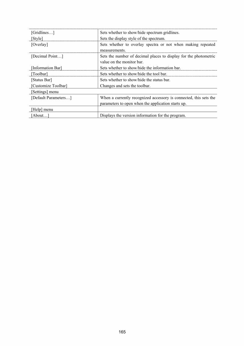
165

[Gridlines…] Sets whether to show/hide spectrum gridlines. [Style] Sets the display style of the spectrum. [Overlay] Sets whether to overlay spectra or not when making repeated

measurements. [Decimal Point…] Sets the number of decimal places to display for the photometric

value on the monitor bar. [Information Bar] Sets whether to show/hide the information bar. [Toolbar] Sets whether to show/hide the tool bar. [Status Bar] Sets whether to show/hide the status bar. [Customize Toolbar] Changes and sets the toolbar. [Settings] menu [Default Parameters…] When a currently recognized accessory is connected, this sets the

parameters to open when the application starts up. [Help] menu [About…] Displays the version information for the program.

166

7.1 [File] Menu Used to save or open measurement results or parameter files. 7.1.1 [Save As…] Saves obtained measurement results to a file.



[Save In] list Select the drive and folder to browse using the drop-down menu. Filenames

saved in the currently open folder are displayed in the filename list. File Name List Select the filename of the data to save. [File Name] Enter the filename of the data to save. The extension may be omitted. The

extension “.jws” is automatically affixed. [Save as type] Sets the files to display in the filename list. Files other than the template file

(.jws) cannot be selected. <Save> Saves the measurement data and closes the dialog. <Cancel> Closes the dialog without saving the measurement data.

7.1.2 [Analysis Send] Transfers the measurement result to the [Spectra Analysis] program. Check the [Send Data to Spectra Analysis] check box in the [Data] tab of the [Measure] menu - [Parameters…] dialog to transfer the spectrum to [Spectra Analysis] automatically after measurement.

Note: This operation can also be performed with the tool button [Analysis Send].

167

7.1.3 [Open Parameters…] Selects a parameter file and opens its parameter.

Note: This operation can also be performed with the tool button [Open Parameter].

Figure 7.3 [Open Parameters] Dialog

[Look in] list Select the drive or folder to browse using the drop-down menu. Filenames

saved in the currently open folder are displayed in the filename list. File Name List Selects the filename of the parameters to be displayed. [File name] Enter the filename of the parameter to be displayed. The extension may be

omitted. The extension “.uvsp” is automatically affixed. The filename can also be selected from the filename list.

[Files of type] Sets the files to display in the filename list. Files other than the template file (.uvsp) cannot be selected.

<Open> Opens the parameter file. <Cancel> Closes the dialog without loading the parameter file.

168

7.1.4 [Save Parameters…] Enter a filename to save currently set measurement parameters.

Note: This operation can also be performed with the tool button [Save Parameters].

Figure 7.4 [Save Parameters] Dialog

[Save In] list Selects the drive and folder to browse using the drop-down menu.

Filenames saved in the currently open folder are displayed in the filename list.

File name list Select the filename of the parameter to save. [File name] Enter the filename of the parameter to save. The extension may be omitted.

The extension “.uvsp” is automatically affixed. [Save as type] Sets the files to display in the filename list. Files other than the template file

(.uvsp) cannot be selected. <Save> Saves the parameter file and closes the dialog. <Cancel> Closes the dialog without saving the parameter file.

169

7.1.5 [Open Baseline…] Selects a baseline file to open. When a baseline file is opened, that baseline is used to correct the sample spectrum.

Figure 7.5 [Open Baseline] Dialog

In the dialog shown in Fig. 7.5, the spectrum of the selected baseline file (see Fig. 7.6) can be viewed by

clicking the <Preview> button .

170

Figure 7.6 [Open Baseline] Dialog

[Look in] list Select the drive or folder to browse using the drop-down menu. Filenames

saved in the currently open folder are displayed in the filename list. File Name List Selects the filename of the baseline to be displayed. [File Name] Enter the filename of the baseline to be displayed. The extension may be

omitted. The extension “.uvsl” is automatically affixed. The filename can also be selected from the filename list.

[Files of type] Sets the files to display in the filename list. Files other than the template file (.vbsl) cannot be selected.

[Preview] Shows details of the selected baseline spectrum (see Fig. 7.6).

<Open> Opens the baseline file. <Cancel> Closes the dialog without loading the baseline file.

171

7.1.6 [Save Baseline ...] Enter a filename to save currently used baseline.

Figure 7.7 [Save Baseline] Dialog



File Name List Selects the filename of the baseline to save. [File Name] Enter the filename of the baseline to save. The extension may be omitted.

The extension “.vbsl” is automatically affixed. [Save as type] Sets the files to display in the filename list. Files other than the template file

(.vbsl) cannot be selected. <Save> Saves the baseline file and closes the dialog. <Cancel> Closes the dialog without saving the baseline file.

172

7.1.7 [Open Dark Spectrum…] Selects a dark file to open. The opened dark spectrum file is used to correct the sample spectrum.

Figure 7.8 [Open Dark Spectrum]

In the dialog shown in Fig. 7.8, the selected dark spectrum (see Fig. 7.9) can be viewed by clicking the

<Preview> button .

173

Figure 7.9 [Open Dark] Dialog

[Look in] list Selects the drive and folder to browse using the drop-down menu.


File Name List Selects the filename of the template to be displayed. [File Name] Enters the filename of the dark data be displayed. The extension may be

omitted. The extension “.vdrk” is automatically affixed. The filename can also be selected from the filename list.

[Files of type] Sets the files to display in the filename list. Files other than template files (.vdrk) cannot be selected.

[Preview] Shows details of the selected dark spectrum (see Fig. 7.9).

<Open> Opens the dark data file. <Cancel> Closes the dialog without loading the dark data file.

174

7.1.8 [Save Dark Spectrum] Enter the filename to save the currently used dark spectrum.

Figure 7.10 [Save Dark Spectrum] Dialog

[Save In] list Selects the drive or folder to browse using the drop-down menu. Filenames

saved in the currently open folder are displayed in the filename list. File Name List Selects the filename of the dark spectrum data to save. [File Name] Enter the filename of the dark spectrum data to save. The extension may be

omitted. The extension “.vdrk” is automatically affixed. [Save as type] Sets the files to display in the filename list. Files other than the template file

(.vdrk) cannot be selected. <Save> Saves the dark data and closes the dialog. <Cancel> Closes the dialog without saving the dark data.

7.1.9 [Exit] Exits the spectra measurement program.

175

7.2 [Measure] Menu Starts and cancels the measurement and sets the measurement parameters. 7.2.1 [Cancel] Cancels the measurement. A dialog to confirm whether or not to validate the measurement data is displayed.

Note: This operation can also be performed with the tool button [Cancel].

Figure 7.11 Stop Dialog

<Yes> Keeps the acquired spectrum data. <No> Discards the acquired spectral data. <Cancel> Continues the measurement.

7.2.2 [Sample] Used for starting sample measurement. Check the [Send Data to Spectra Analysis] check box to transfer the data to the [Spectra Analysis] program after measurement, which displays the measured spectrum in a new View.

Note: This operation can also be performed with the tool button [Sample].

176

7.2.3 [Baseline] Available when [Baseline] or [Baseline/Dark] correction is selected in the [Settings] - [Parameters…] - [Control] tab, [Correction] item. Confirm that there is nothing in the sample compartment or that the sample for the baseline measurement is inserted and then press the <Measure> button.

Note: This operation can also be performed with the tool button [Baseline].

Figure 7.12 [Baseline Measurement] Dialog

<Measure> The baseline measurement starts. <Cancel> The baseline measurement is not performed and the [Baseline

Measurement] dialog box closes. 7.2.4 [Dark] Available if [Baseline/Dark] correction is selected in the [Measure] - [Parameters] - [Control] tab, [Correction] item. Block off the optical path of the sample side of the sample compartment with a shield and then press the <Measure> button.

Note: This operation can also be performed with the tool button [Dark].


<Measure> The dark measurement starts. <Cancel> The dark measurement is not performed and the [Dark Measurement]

dialog box closes.

177

7.2.5 [Parameters…] Sets the measurement parameters. This dialog has four tabs for setting: Basic, Control, Information and Data. These tabs can be changed by clicking the tab for each item at the top of the dialog. The parameters can be switched between two modes: basic mode that automatically sets parameters using basic combination and advanced mode that assigns each parameter individually. <Basic/Advanced> Toggles between Basic and Advanced modes. <Open…> Loads a measurement parameter file. <Save…> Saves the measurement parameters as a file (extension “. uvsp”) <Default> Sets the General/Control parameters to their default values and resets the

info/data to their previous settings. <OK> Sets the parameter and closes the dialog. <Cancel> Closes the dialog without setting the parameter.

Note: This operation can also be performed with the tool button [Parameter]. 7.2.5.1 [General] tab

Figure 7.14 [Parameters Basic] Dialog, [General] Tab (Basic mode)

178

Figure 7.15 [Parameters Advanced] Dialog, [General] Tab (Advanced mode)

Basic mode [Photometric Mode] Selects the photometric mode.

Options: ▪ Abs: Absorbance measurement ▪ %T: Transmittance measurement ▪ %R: Reflectance measurement

[Bandwidth] The selectable range varies depending on the model. V-630 : 1.5 nm V-650/660 : 2 nm V-670 : 2 nm (UY/Vis region), 8 nm (NIR region)

[Response] Response determined by simple moving average. The options vary depending on the model. V-630 : ▪ VQuick: Moving average over approx. 0.015 sec ▪ Quick: Moving average over approx. 0.06 sec ▪ Fast: Moving average over approx. 0.25 sec ▪ Medium: Moving average over approx. 1 sec ▪ Slow: Moving average over approx. 4 sec V-650/660/670 : ▪ Quick: Moving average over approx. 0.06 sec ▪ Fast: Moving average over approx. 0.25 sec ▪ Medium: Moving average over approx. 1 sec ▪ Slow: Moving average over approx. 4 sec Note: Refer to Tables 7.2 and 7.3 for response and scanning

speed and data pitch interval combinations.

[Scan] This is the wavelength scanning speed.

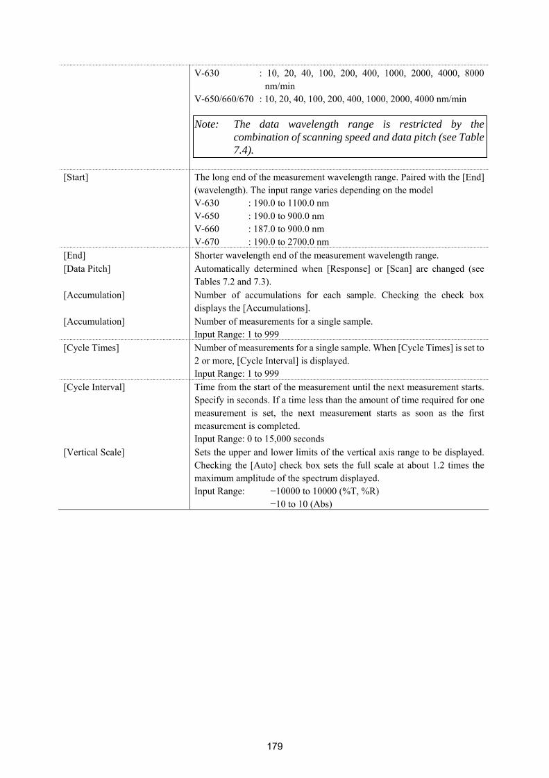
179

V-630 : 10, 20, 40, 100, 200, 400, 1000, 2000, 4000, 8000 nm/min

V-650/660/670 : 10, 20, 40, 100, 200, 400, 1000, 2000, 4000 nm/min Note: The data wavelength range is restricted by the

combination of scanning speed and data pitch (see Table 7.4).

[Start] The long end of the measurement wavelength range. Paired with the [End]

(wavelength). The input range varies depending on the model V-630 : 190.0 to 1100.0 nm V-650 : 190.0 to 900.0 nm V-660 : 187.0 to 900.0 nm V-670 : 190.0 to 2700.0 nm

[End] Shorter wavelength end of the measurement wavelength range. [Data Pitch] Automatically determined when [Response] or [Scan] are changed (see

Tables 7.2 and 7.3). [Accumulation] Number of accumulations for each sample. Checking the check box

displays the [Accumulations]. [Accumulation] Number of measurements for a single sample.

Input Range: 1 to 999 [Cycle Times] Number of measurements for a single sample. When [Cycle Times] is set to

2 or more, [Cycle Interval] is displayed. Input Range: 1 to 999

[Cycle Interval]

Time from the start of the measurement until the next measurement starts. Specify in seconds. If a time less than the amount of time required for one measurement is set, the next measurement starts as soon as the first measurement is completed. Input Range: 0 to 15,000 seconds

[Vertical Scale] Sets the upper and lower limits of the vertical axis range to be displayed. Checking the [Auto] check box sets the full scale at about 1.2 times the maximum amplitude of the spectrum displayed. Input Range: −10000 to 10000 (%T, %R) −10 to 10 (Abs)

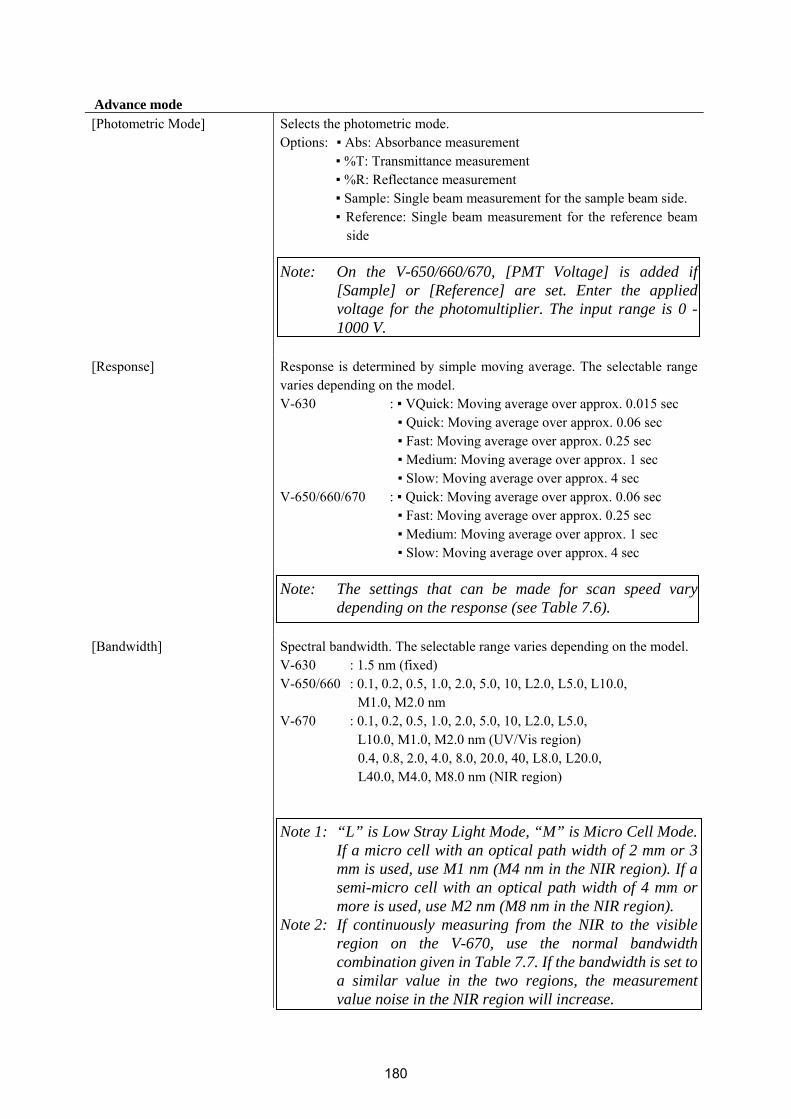
180

Advance mode [Photometric Mode] Selects the photometric mode.

Options: ▪ Abs: Absorbance measurement ▪ %T: Transmittance measurement ▪ %R: Reflectance measurement ▪ Sample: Single beam measurement for the sample beam side. ▪ Reference: Single beam measurement for the reference beam

side Note: On the V-650/660/670, [PMT Voltage] is added if

[Sample] or [Reference] are set. Enter the applied voltage for the photomultiplier. The input range is 0 - 1000 V.

[Response] Response is determined by simple moving average. The selectable range

varies depending on the model. V-630 : ▪ VQuick: Moving average over approx. 0.015 sec ▪ Quick: Moving average over approx. 0.06 sec ▪ Fast: Moving average over approx. 0.25 sec ▪ Medium: Moving average over approx. 1 sec ▪ Slow: Moving average over approx. 4 sec V-650/660/670 : ▪ Quick: Moving average over approx. 0.06 sec ▪ Fast: Moving average over approx. 0.25 sec ▪ Medium: Moving average over approx. 1 sec ▪ Slow: Moving average over approx. 4 sec Note: The settings that can be made for scan speed vary

depending on the response (see Table 7.6).

[Bandwidth]

Spectral bandwidth. The selectable range varies depending on the model. V-630 : 1.5 nm (fixed) V-650/660 : 0.1, 0.2, 0.5, 1.0, 2.0, 5.0, 10, L2.0, L5.0, L10.0,

M1.0, M2.0 nm V-670 : 0.1, 0.2, 0.5, 1.0, 2.0, 5.0, 10, L2.0, L5.0, L10.0, M1.0, M2.0 nm (UV/Vis region)

0.4, 0.8, 2.0, 4.0, 8.0, 20.0, 40, L8.0, L20.0, L40.0, M4.0, M8.0 nm (NIR region)

Note 1: “L” is Low Stray Light Mode, “M” is Micro Cell Mode.

If a micro cell with an optical path width of 2 mm or 3 mm is used, use M1 nm (M4 nm in the NIR region). If a semi-micro cell with an optical path width of 4 mm or more is used, use M2 nm (M8 nm in the NIR region).

Note 2: If continuously measuring from the NIR to the visible region on the V-670, use the normal bandwidth combination given in Table 7.7. If the bandwidth is set to a similar value in the two regions, the measurement value noise in the NIR region will increase.

181

[Scan] This is the wavelength scanning speed.

V-630: 10, 20, 40, 100, 200, 400, 1000, 2000, 4000, 8000 nm/min V-650/660/670: 10, 20, 40, 100, 200, 400, 1000, 2000, 4000 nm/min Note: The data intervals that can be set vary depending on the

scanning speed (see Table 7.6)

[Start] The long end of the measurement wavelength region. Paired with the [End] (wavelength). The input range varies depending on the model V-630 : 190.0 to 1100.0 nm V-650 : 190.0 to 900.0 nm V-660 : 187.0 to 900.0 nm V-670 : 190.0 to 2700.0 nm

[End] Shorter wavelength end of the measurement wavelength range. [Data Pitch] Data collecting wavelength interval. Selectable range varies depending on

the model. V-630 : 0.1, 0.2, 0.5, 1, 2, 5 nm V-650/660 : 0.025, 0.05, 0.1, 0.2, 0.5, 1, 2, 5 nm V-670 : When [Scan Mode] is set to [Continuous] 0.025, 0.05, 0.1, 0.2, 0.5, 1, 2, 5 nm (For UV/VIS region

measurements only) 0.1, 0.2, 0.5, 1, 2, 5 nm (measurements include the NIR

region) When [Scan Mode] is [Step] 0.1, 0.2, 0.5, 1, 2, 5 nm (measurements only for the UV/Vis

region) 0.5, 1, 2, 5 nm (measurements include the NIR region) Note: The measurement wavelength range is restricted by the

[Data Pitch] (see Table 7.4).

[Scan Mode] Sets the scan mode. If [Continuous] is selected, measurements are made with a continuous scan. If [Step] is selected, measurements are made with a step scan.

[Accumulation] Performs accumulated measurements for a single sample. Check the check box to display [Accumulation Times].

[Accumulation] Number of measurements for a single sample. Input Range: 1 to 999

[Cycle Times] Number of measurements for a single sample. When [Cycle Times] is set to 2 or more, the [Cycle Interval] is displayed. Input Range: 1 to 999

[Cycle Interval]

Time from the start of the measurement until the next measurement starts. Specify in seconds. If a time less than the amount of time required for one measurement is set, the next measurement starts as soon as the first measurement completed. Input Range: 0 to 15,000 seconds

[Vertical Scale] Sets the upper and lower limits of the vertical axis range to display on the screen. Check the checkbox to set the full scale to approximately 1.2 times

182

the maximum width of the displayed spectrum, in accordance with the measurement results. Input Range: −10000 to 10000 (%T, %R) 0 to 100 (Sample, Reference) −10 to 10 (Abs)

Basic Mode Combination

Table 7.2 When Response is specified

Response Scanning Speed (nm/min) Data Pitch (nm) VQuick* 8000 5

Quick 2000 1 Fast 1000 0.5

Medium 200 0.2 Slow 40 0.1

*VQuick can only be set on the V-630

Table 7.3 When Scanning Speed is specified Scanning Speed (nm/min) Response Data Pitch (nm)

8000 Quick, VQuick 5 4000 Quick, VQuick 2 2000 Quick 1 1000 Fast 0.5 400 Fast 0.5 200 Medium 0.2 100 Medium 0.1 40 Slow 0.1 20 Slow 0.1 10 Slow 0.1

Table 7.4 [Data Pitch] and [Measurement Wavelength Range] Combination

Combination of [Data interval] and [Data Pitch] Data Pitch (nm) Maximum Measurement

Wavelength Range (nm) 0.025* 750 0.05* 1500

0.1 and over Entire range can be measured. *On the V-630, there are no data intervals of 0.025 nm or 0.05 nm.

183

Advanced Mode Combination

Table 7.5 [Scanning Speed] and [Data Pitch] Combination Data Pitch (nm) 0.025* 0.05* 0.1 0.2 0.5 1 2 5 Scanning Speed

(nm/min)

10 √ √ √ √ √ √ √ √ 20 √ √ √ √ √ √ √ √ 40 √ √ √ √ √ √ √ √ 100 × √ √ √ √ √ √ √ 200 × × √ √ √ √ √ √ 400 × × × √ √ √ √ √

1000 × × × × √ √ √ √ 2000 × × × × × √ √ √ 4000 × × × × × × √ √ 8000 × × × × × × × √

*On the V-630, there are no data intervals of 0.025 nm or 0.05 nm.

Table 7.6 [Scanning Speed] and [Response] Combination Response VQuick* Quick Fast Medium Slow

Scanning Speed (nm/min)

10 √ √ √ √ √ 20 √ √ √ √ √ 40 √ √ √ √ √ 100 √ √ √ √ √ 200 √ √ √ √ √ 400 √ √ √ √ ×

1000 √ √ √ √ × 2000 √ √ √ × × 4000 √ √ √ × × 8000 √ √ × × ×

*VQuick can be set only on the V-630

Table 7.7 UV/VIS Region/NIR Region Bandwidth Combination UV/VIS Region Bandwidth (UV) nm Near Infrared Region Bandwidth (NIR) nm

0.1 0.2 0.5 1

2 (L10) 5 (L10)

10 (L10) M1 M2

0.4 0.8 2 4

8 (L8) 20 (L20) 40 (L40)

M4 M8

184

7.2.5.2 [Control] tab

Figure 7.16 [Parameters Basic] Dialog, [Control] Tab (Basic Mode)

Figure 7.17 [Parameters Advanced] Dialog, [Control] Tab (Advanced mode)

185

Basic mode Baseline Correction [None] Select when baseline correction is not performed. [Baseline] Select when baseline correction is performed. Changeover wavelength [Light Source] Sets the changeover wavelength for the deuterium lamp and halogen lamp.


[Grating/Detector] Sets the changeover wavelength for the photomultiplier and PbS. Enter a wavelength in the text box. Input range: 750 to 900 nm (default setting: 800 nm) Note: The [Grating] changeover wavelength can only be set on

the V-670.

Advance mode Baseline Correction [None] Select when baseline correction is not performed. [Baseline] Select when baseline correction is performed. [Baseline/Dark] Select this when both baseline and dark corrections are performed. [Changeover wavelength] [Light Source] Sets the changeover wavelength for the deuterium lamp and halogen lamp.


[Grating/Detector]

Sets the photomultiplier and PbS changeover wavelength. Enter a wavelength in the text box. Input range: 750 to 900 nm (default setting: 800 nm) Note: The [Grating/Detector] changeover wavelength is only a

setting item for the V-670.

Light Source [Auto] Select this when both the deuterium and halogen lamp light sources are

used during measurement. [Deuterium Lamp] Select this when only the deuterium lamp light source is used during

measurement. [Halogen Lamp] Select this when only the halogen lamp light source is used during

measurement. [External Source] Select this when measuring with a light source other than the internal

deuterium lamp or halogen lamp. Filter exchange [Continue Scan]

Changes the filter without stopping the scan.

186

[Stop scan]

Changes the filter by stopping the scan Note: If the filter is changed without stopping the scan, the

measurement time can be shortened, but noise may appear at the filter changeover wavelength as indicated in Fig. 7.18.

98

102

99

100

101

190 27001000 2000

%T

Wavelength [nm] Figure 7.18 (Top) Filter changeoever without stopping the scan.

(Bottom) Scan is stopped and filter changed.

187

7.2.5.3 [Information] tab

Figure 7.19 [Parameters Basic] Dialog, [Information] Tab

[Sample Name] Enter the sample name (maximum of 63 single-byte characters). [Operator] Enter the name of operator (maximum of 63 single-byte characters). [Division] Enter the division of operator (maximum of 127 single-byte characters). [Comment] Enter a comment. Use as required (maximum of 127 single-byte

characters). [Display the [Comment] dialog box before taking measurement]

Sets whether to display the information dialog for each measurement.

188

7.2.5.4 [Data] tab


[Save Data] Automatically saves data. A filename is automatically allocated to the

measured spectrum data and automatically saved to the specified directory.[Auto Save] Toggles the auto saving function ON/OFF. [Save in] Displays the drive and folder name for saving data. <Browse…> The save-in drive and folder name can be referred to. [Format] Sets the filename to be assigned in auto saving. The file format is the

standard file (extension “jws”). [Date-No.] Sets [Date] + [3-digit serial number] as filename. The date and serial

number are connected with a hyphen “ - ” . [Sample-No.] Sets [Sample name] + [3-digit serial number] as the filename. The [Sample

Name] is the name entered in the [Information] tab. [Comment-No.] Sets [Comment] + [3 digit serial number] as filename. The [Comment] is

the comment entered in the [Information] tab. [Sample-Comment-No.] Sets [Sample name] + [Comment] + [3-digit serial number] as filename.

The [Sample] and [Comment] are the names and comments entered in the [Information] tab, respectively.

[String-No.] Sets [String-No.] + [3-digit serial number] as filename. Enter the character string in the text box below (maximum one-byte 63 characters).

[String] Can be entered when a character string is selected with [Format] (maximum of 63 characters).

[Send to Analysis] Sets whether to automatically send to [Spectra Analysis] after performing measurement.

[Send Data to Spectra Analysis]

Sets when automatically sending to [Spectra Analysis] after measurement is complete. For [Repeat Measurement], data is sent after each single scan

189

is completed. [Print] Sets whether to automatically print after measurement is complete. [Print Measured Data] Sets whether to automatically print after measurement is complete. For

[Repeat Measurement], data is printed after each single scan is completed.[Template] The drive and filename to which the print template file was saved is

displayed. <Browse…> The drive and filename to which the print template file is saved can be

selected by using the browse function. 7.2.6 [Preview…] Previews sample spectrum. For details about setting and using Preview, see Chapter 6 [Quantitative Measurement] Program Reference, Section 6.1.2.6 [Preview…].

7.3 [Control] Menu 7.3.1 [Move Wavelength…] Moves the wavelength of the spectrophotometer to the desired wavelength.


[Move To] Text box for entering the wavelength.



Note: This operation can also be performed with the tool button [Move Wavelength].

190

7.3.2 [Optical Path] The [Optical Path] is a function for observing the optical path when changing the light source to the zero-order of the halogen lamp. When the [Optical Path] command is selected, the [Optical Path Check] dialog is displayed (see Fig. 7.22) and the switch to the zero-order halogen lamp is performed. Once the switch to zero-order has been completed, Fig. 7.23 is displayed and the bandwidth can be changed to monitor the optical path. Clicking the <OK> button displays Fig. 7.24, and the status of the bandwidth and wavelength return to the state they were in before the [Optical Path Check] command was executed.




[Band Width] Sets the bandwidth. The selectable range varies depending on the model.

V-630 : 1.5 nm (fixed) V-650/660/670 : 0.1、0.2、0.5、1.0、2.0、5.0、10、L2.0、L5.0、L10.0、

M1.0、M2.0 nm <OK> The [Optical Path Check] dialog box closes and the bandwidth and

wavelength return to the state they were in before the [Optical Path Check] command was executed.

Note: This operation can also be performed with the tool button [Optical Path Check].

191

7.3.3 [Band Width] Changes the currently monitored bandwidth. When starting a measurement, the actual measurement starts once the bandwidth returns to the value set in [Parameters]. Note 1: The [Band Width] command is not displayed on the V-630. Note 2: On the V-670, the bandwidths that can be set vary depending on whether the current

wavelength is in the UV/Vis region or the NIR region.

Figure 7.25 [Band Width] Popup Menu (UV/Vis Region)

Figure 7.26 [Band Width] Popup Menu (NIR Region)


192

7.3.4 [Response] Changes the currently monitored response. When starting a measurement, the actual measurement starts once the response returns to the value set in [Parameters].


Note 1: This operation can also be performed with the tool button [Response]. Note 2: The VQuick setting is also possible on the V-630. 7.3.5 [Light Source] Displays the lamp use time and toggles the lamp on/off. When starting a measurement, the actual measurement starts once the lamp status returns to the status set in [Parameters].



closes.

Note 1: Turning the light ON/OFF can also be performed with the tool button

[Deuterium lamp] and [Halogen lamp]. Note 2: It takes approximately 5 minutes for the light source to stabilize. Refrain from taking a


193

7.3.6 [Auto Zero] Sets the absorbance value (or transmittance) of the current wavelength to zero (100%T in transmittance).


Note: This operation can also be performed with the tool button [Auto Zero]. 7.3.7 [Select Accessory…] Manually registers accessories that are not automatically detected. Select the accessory to be used and click the <OK> button. The [Accessory has been attached] dialog is displayed and a list of registered startup applications is displayed. For further details, see Section 3.5 “Manually Detecting Accessories”.


Note: If an auto-detect accessory is connected, the [Select Accessory] command cannot be

used.

194

7.4 [View] Menu Used for setting the display. 7.4.1 [Scale…] Changes the display scale of the spectrum.


Horizontal Axis Scale Enters the scale of the horizontal axis. Checking the [Auto] check box

displays the entire range ignoring the input values. Vertical Axis Scale Enters the scale of the vertical axis. Marking the [Auto] check box



195

7.4.2 [Pattern…] Sets the display color and line style of the spectrum.


[Element] list Select an element to change colors and line styles of spectra 1 - 8, frames,

grid lines and auxiliary grid lines. [Color] Changes the color of the element selected in the [Element] list. [Line Style] Sets the line format of the element selected from the [Element] list. [Line Width] Sets the line width. [Sample] Displays a sample of the designated style. [Set As Default] Check this check box to apply the subsequent display.

Note: This operation can also be performed with the tool button [Pattern].

196

7.4.3 [Font…] Designates the display font.


[Item] Selects items to set the font for.


[Vertical Label Orientation] Selects the orientation in which the axis label is to be displayed. [Horizontal]: Horizontal to the spectrum display window [Vertical]: Vertical to the spectrum display window


<Save> Opens the [Font] dialog.




197

[Font] Selects a font. [Style] Selects a fonts style. [Size] Selects a font size. [Effects] Strikeout and underline can be specified. [Color] list Selects the font color. [Sample] Displays a sample of the specified font. [Script] Selects the language for the specified font. <OK> Sets the font and returns to the [Font] dialog. <Cancel> Returns to the [Font] dialog without applying font settings.

Note: This operation can also be performed with the tool button [Font]. 7.4.4 [Gridlines…] Sets whether to show/hide grid lines.



Note: This operation can also be performed with the tool button [Gridlines].

198

7.4.5 [Style…] Sets the spectrum display style.


[Axis] Select the setting form of the vertical or horizontal axis. [Scale label] [Interval: Auto] Check this check box to set the scale display method “Automatic”. [Interval: Manual] Check this check box to set the scale display to the desired interval. In


[Decimals Point on Scale Label]



Note: This operation can also be performed with the tool button [Style]. 7.4.6 [Overlay] Sets whether to overlay the spectra in the spectrum measurement screen when making repeated measurements.

199

7.4.7 [Decimal Point…] Sets the number of decimal places to display for the photometric value on the monitor bar.


[Item] list Selects the items to change (absorbance, transmittance, reflectance, sample,

reference). [Format] Sets the number of decimal places to display for the selected items in the

[Item] list.

Note: This operation can also be performed with the tool button [Decimal Point]. 7.4.8 [Information Bar] Sets whether to show/hide the information bar. 7.4.9 [Toolbar] Sets whether to show/hide the tool bar. [File] Used for selecting whether to show/hide the tool bar corresponding to the

pull-down menu files. [Measure] Used for selecting whether to show/hide the tool bar corresponding to the

pull-down menu measurements. [Control] Used for selecting whether to show/hide the tool bar corresponding to the

pull-down menu control. [View] Used for selecting whether to show/hide the tool bar corresponding to the

pull-down menu view. 7.4.10 [Status bar] Sets whether to show/hide the status bar

200

7.4.11 [Customize Toolbar…] Sets whether to show/hide and makes changes to the toolbar.


[File] Shows/hides the toolbars corresponding to the [File] menu and

adds/removes the tool buttons that appear.

Button Name

[Save As]

[Analysis Send]

[Open parameters]

[Save parameters]

[Measure] Shows/hides the toolbars corresponding to the [Measure] menu and


Button Name

[Cancel]

[Sample]

[Baseline]

[Dark]

[Parameters]

[Preview]

[Control] Shows/hides the toolbars corresponding to the [Control] menu and


Button Name

[Move wavelength]

[Optical Path]

[Band width]

[Response]

201

[Toggle Deuterium lump]

[Toggle Halogen lump]

[Auto Zero]

[View] Shows/hides the toolbars corresponding to the [View] menu and


Button Name

[Scale]

[Pattern]

[Font]

[Gridlines]

[Style]

[Decimal Point]

[View Name] If this checkbox is marked, the button names are displayed under each

toolbar button. <Customize> Click this button to start up a dialog to customize the toolbar (see Fig. 7.39).


202

7.5 [Settings] Menu 7.5.1 [Default Parameters…] Sets the parameters at program startup when using the Spectra Measurement program with the currently connected accessory. Multiple accessories can be set. Connect and configure each accessory.


[Open the most recently used parameters]

Starts with the parameters set just prior to exiting the Spectra Measurement program.

[Open the specified parameter file] Starts with the specified parameter file. [File Name] Available when using [Open the specified parameter file].

7.6 Help] Menu 7.6.1 [About] Displays version information for this spectra measurement program.

203

8 [Time course measurement] Program Reference The Time Course Measurement program measures the changes to a sample’s absorbance, transmittance and reflectance over time at a fixed wavelength. Start up the time course measurement program to open the following window.

Figure 8.1 [Time Course Measurement] Window

Toolbar Common functions for measurement, parameter settings and others can be accessed with the buttons on this toolbar (see Table 8.1). The tool buttons can be customized in the [View] menu.

Monitor bar Displays the current wavelength, photometric value and measurement time.

Information bar Displays the current measurement parameters and accessory information.

Time course data display fieldDisplays the time course data being measured. The display format can be set using the [View] menu.

204


[Save Data] 8.1.1 [Save Data…]

[Analysis Send] 8.1.2 [Analysis Send]

[Open Parameters] 8.1.3 [Open parameters…]

[Save Parameters] 8.1.4 [Save Parameters…]


[Sample Measurement] 8.2.2 [Sample]

[Blank Measurement] 8.2.3 [Blank]

[Dark Measurement] 8.2.4 [Dark]





[Band Width] 8.3.3 [Band Width]


[Toggle Deuterium Lamp] 8.3.5 [Light Source…]

[Toggle Halogen lamp] 8.3.5 [Light Source…]


[Scale] 8.4.1 [Scale…]

[Pattern] 8.4.2 [Pattern…]

[Font] 8.4.3 [Font…]

[Gridlines] 8.4.4 [Gridlines…]

[Style] 8.4.5 [Style…]


205

Window Title bar Displays the program window name. Menu bar Displays the names of menus that can be used. Monitor bar Displays the wavelength, photometric value and measurement time from left

to right Tool bar Displays icons of available tools. The Tool buttons can be customized in the

[View] menu. Information bar Displays current measurement parameters and accessory information. Time Course Data Display Monitors time course data during measurement. Status bar Displays information about the instrument status and explanations of

selected menus. Menu [File] menu [Save Data…] Saves a time course data under a new file name. [Analysis Send] Transfers the measurement result to the spectra analysis program. [Open Parameters...] Selects a parameter file and opens those parameters. [Save Parameters...] Saves parameters using entered filename. [Exit] Exits the time course measurement program and returns to [Spectra

Manager]. [Measure] menu [Cancel] Cancels the measurement. [Sample] Starts the sample measurement. [Blank] Measures data for blank correction. [Dark] Measures data for dark correction. [Parameters...] Sets parameters. [Preview...] Sets the measurement parameters and previews the spectrum shape. [Control] menu [Move Wavelength...] Moves the wavelength of the spectrophotometer to the desired wavelength. [Optical Path...] Changes to zero-order light for checking the optical path. [Band Width] Changes the bandwidth. [Response] Changes the currently monitored response. [Light Source...] Switches the light source on/off. [Auto Zero] Sets the absorbance value (or transmittance) of the current wavelength to zero

(100%T for transmittance). [Select Accessory...] Selects an accessory. [View] Menu [Scale...] Changes the display scale of time course data. [Pattern...] Sets the display color and line style of time course data. [Font...] Designates the display font for time course data. [Gridlines...] Sets whether to show/hide of grid lines for time course data. [Style...] Sets the display style for the time course data. [Decimal Point...] Sets the number of decimal places to display for the photometric value on the

monitor bar. [Information Bar] Sets whether to show/hide the information bar. [Toolbar] Sets whether to show/hide of the toolbar. [Status Bar] Sets whether to show/hide of the status bar. [Customize Toolbar...] Changes and sets the toolbar.

206

[Setting] menu [Default Parameters…] When a currently recognized accessory is connected, sets the parameters to

open when the application starts up. [Help] Menu [About...] Displays the version information for the program.

8.1 [File] Menu Used to save or open measurement results or parameter files. 8.1.1 [Save Data…] Saves obtained measurement results to a file.

Note: This operation can also be performed using the tool button [Save Data]


[Save in] List Select the drive and folder to browse using the drop-down menu. Filenames

saved in the currently open folder are displayed in the filename list. File Name List Select the filename of the data to save. [File Name] Enter the filename of the data to save. The extension may be omitted. The

extension “.jws” is automatically affixed. [Save as type] Sets the files to display in the filename list. Files other than the template file

(.jws) cannot be selected. <Save> Saves the measurement data and closes the dialog. <Cancel> Closes the dialog without saving the measurement data.

8.1.2 [Analysis Send] Transfers the measurement result to the [Spectra Analysis] program. Check the [Send Data to Spectra Analysis] check box in the [Data] tab of the [Measure] menu - [Parameters…] dialog to transfer the spectrum to [Spectra Analysis] automatically after measurement.

Note: This operation can also be performed with the tool button [Analysis Send].

207

8.1.3 [Open Parameters…] Selects a parameter file and opens its parameters.

Note: This operation can also be performed with the tool button [Open Parameters].


[Look in] List Select the drive or folder to browse using the drop-down menu. Filenames saved in the currently open folder are displayed in the filename list.

File Name List Selects the filename of the parameters to be displayed. [File Name] Enter the filename of the parameters to be displayed. The extension may be

omitted. The extension “.uvtm” is automatically affixed. The filename can also be selected from the filename list.

[File Type] Sets the files to display in the filename list. Files other than the template file (.uvtm) cannot be selected.


208

8.1.4 [Save Parameters…] Enter a filename to save the currently set measurement parameters.





File Name List Select the filename of the parameters to save. [File Name] Enter the filename of the parameters to save. The extension may be

omitted. The extension “.uvtm” is automatically affixed. [File Type] Sets the files to display in the filename list. Files other than the template file

(.uvtm) cannot be selected. <Save> Saves the parameter file and closes the dialog. <Cancel> Closes the dialog without saving the parameter file.

8.1.5 [Exit] Exits the time course measurement program.

209

8.2 [Measure] Menu Starts and cancels the measurement and sets measurement parameters. 8.2.1 [Cancel] Cancels the measurement. A dialog to confirm whether or not to validate the measurement data is displayed.

Note: This operation can also be performed with the tool button [Cancel].

Figure 8.5 Stop Dialog

<Yes> Keeps the measured spectral data. <No> Discards the measured spectral data. <Cancel> Continues the measurement.

8.2.2 [Sample] Used for starting sample measurement. Check the [Send Data to Spectra Analysis] check box to transfer the data to the [Settings] - [Parameters…] - [Data] Tab, [Send] item to the [Spectra Analysis] program after measurement, which displays the measured spectrum in a new View.

Note: This operation can also be performed with the tool button [Sample].

210

8.2.3 [Blank] Used for measurement of a blank sample. Available when [Blank] or [Blank/Dark] is selected in the [Measurement] - [Parameters] - [Control] tab, [Correction] item. Confirm that there is nothing in the sample compartment or that the sample for the blank measurement is inserted and then press the <Measure> button.




dialog box closes. 8.2.4 [Dark] Used for starting the dark measurement. Available if [Blank/Dark Correction] is selected in the [Measure] - [Parameters…] - [Control] Tab, [Correction] item. Block off the optical path of the sample side of the sample compartment with a shield and then press the <Measure> button.




dialog box closes.

211

8.2.5 [Parameters…] Sets the measurement parameters. This dialog has four tabs for setting, Basic, Control, Information and Data. These tabs can be changed by clicking the tab for each item at the top of the dialog. The parameters can be switched between two modes: basic mode that automatically sets parameters using basic combination and advanced mode that assigns each parameter individually.

<Basic/Advanced> Toggles between Basic and Advanced modes. <Open...> Loads a measurement parameter file. <Save...> Saves the measurement parameters as a file (extension “.uvtm”). <Default> Sets the General/Control parameters to their default values, and resets the

info/data to their previous settings. <OK> Sets the parameter and closes the dialog. <Cancel> Closes the dialog without setting the parameter.



212

Figure 8.9 [Parameters Advanced] Dialog, [General] Tab (Advanced mode) Basic mode [Photometric Mode] Selects the photometric mode.

Selectable Range: ▪ Abs: Absorbance measurement ▪ %T: Transmittance measurement ▪ %R: Reflectance measurement

[Response] Response determined by simple moving average. The options vary depending on the model. V-630 : ▪ VQuick: Moving average over approx. 0.015 sec ▪ Quick: Moving average over approx. 0.06 sec ▪ Fast: Moving average over approx. 0.25 sec ▪ Medium: Medium: Moving average over approx. 1 sec ▪ Slow:Slow: Moving average over approx. 4 sec V-650/660/670 : ▪ Quick: Moving average over approx. 0.06 sec ▪ Fast: Moving average over approx. 0.25 sec ▪ Medium: Moving average over approx. 1 sec ▪ Slow: Moving average over approx. 4 sec

[Band Width] The selectable range varies depending on the model. V-630 : 1.5 nm V-650/660 : 2 nm V-670 : 2 nm (UV/Vis region), 8 nm (NIR region)

[Wavelength] Indicates the wavelength. The input range varies depending on the model. V-630 : 190.0 to 1100.0 nm V-650 : 190.0 to 900.0 nm V-660 : 187.0 to 900.0 nm V-670 : 190.0 to 2700.0 nm

213

[End] Time to complete the measurement. Can be set from 0.5 to 1500 sec. [Data Pitch] Indicates the data pitch. The input range varies depending on the model.

V-630 : 0.01 sec, 0.02 sec, 0.05 sec, 0.1 sec, 0.2 sec, 0.5 sec, 1.0 sec, 2.0 sec, 5.0 sec, 10.0 sec, 20.0 sec, 30.0 sec, 60.0 sec, 120.0 sec, 300 sec, 600 sec V-650/660/670 : 0.05 sec, 0.1 sec, 0.2 sec, 0.5 sec, 1.0 sec, 2.0 sec, 5.0 sec, 10.0 sec, 20.0 sec, 30.0 sec, 60.0 sec, 120.0 sec, 300 sec, 600 sec

[Vertical Scale] Sets the upper and lower limits of the vertical axis range to be displayed. Checking the [Auto] check box sets the full scale at about 1.2 times the maximum amplitude of the spectrum displayed.

Input range : －10000 to 10000 (%T, %R) －10 to 10 (Abs)

Advanced Mode Selects the photometric mode.

Options: ▪ Abs: Absorbance measurement ▪ %T: Transmittance measurement ▪ %R: Reflectance measurement ▪ Sample: Single beam measurement for the sample beam side. ▪ Reference: Single beam measurement for the reference

beam side Note: On the V-650/660/670, [PMT Voltage] is added if

[Sample] or [Reference] are set. Enter the applied voltage for the photomultiplier. The input range is 0 to 1000 volts.

[Response] Response by simple moving average. The selectable range varies

depending on the model. V-630 : ▪ VQuick: Moving average over approx. 0.015 sec ▪ Quick: Moving average over approx. 0.06 sec ▪ Fast: Moving average over approx. 0.25 sec ▪ Medium: Moving average over approx. 1 sec ▪ Slow: Moving average over approx. 4 sec V-650/660/670 : ▪ Quick: Moving average over approx. 0.06 sec ▪ Fast: Moving average over approx. 0.25 sec ▪ Medium: Moving average over approx. 1 sec ▪ Slow: Moving average over approx. 4 sec

[Band Width] Spectral bandwidth. The selectable range varies depending on the model. V-630 : 1.5 nm (fixed) V-650/660 : 0.1, 0.2, 0.5, 1.0, 2.0, 5.0, 10, L2.0, L5.0, L10.0, M1.0, M2.0 nm V-670 : 0.1, 0.2, 0.5, 1.0, 2.0, 5.0, 10, L2.0, L5.0, L10.0, M1.0, M2.0 nm (UV/Vis region) 0.4, 0.8, 2.0, 4.0, 8.0, 20.0, 40, L8.0, L20.0, L40.0, M4.0, M8.0 nm (NIR region)

214

Note 1: “L” is Low Stray Light Mode, “M” is Micro Cell Mode. If a micro cell with an optical path width of 2 mm, 3 mm is used, use M1 nm (M4 nm in the NIR region). If a semi-micro cell with an optical path width of 4mm or more is used, use M2 nm (M8 nm in the NIR region).

Note 2: If continuously measuring from the NIR to the visible

region on the V-670, use the normal bandwidth combination given in Table 8.2. If the bandwidth is set to a similar value for the two regions, the measurement value noise in the NIR region will increase.

[Wavelength] Indicates the measurement wavelength. The input range varies depending

on the model. V-630 : 190.0 to 1100.0 nm V-650 : 190.0 to 900.0 nm V-660 : 187.0 to 900.0 nm V-670 : 190.0 to 2700.0 nm

[Interval] Data collecting wavelength interval. Selectable range varies depending on the model. V-630 : 0.01 sec, 0.02 sec, 0.05 sec, 0.1 sec, 0.2 sec, 0.5 sec, 1.0 sec, 2.0 sec, 5.0 sec, 10.0 sec, 20.0 sec, 30.0 sec, 60.0 sec, 120.0 sec, 300 sec, 600 secV-650/660/670 : 0.05 sec, 0.1 sec, 0.2 sec, 0.5 sec, 1.0 sec, 2.0 sec, 5.0 sec, 10.0 sec, 20.0 sec, 30.0 sec, 60.0 sec, 120.0 sec, 300 sec, 600 sec Note: To delete an existing step, right-click the number of the

step to be deleted. The window in Figure 8.10 is displayed.

Figure 8.10 Deleting a Step Number

[End Time] Time to complete measurement. Set the number of data points from 11 to 30001.

[Vertical Scale] Sets the upper and lower limits of the vertical axis range to display on the screen. Check the [Auto] checkbox to set the full scale at approximately 1.2 times the maximum width of the displayed spectrum. Input range : −10000 to 10000 (%T, %R) 0 to 100 (Sample, Reference) −10 to 10 (Abs)

[Unit of Time] Set the unit of time for the horizontal axis. sec: Sets the units for the horizontal axis as seconds. min. Sets the units for the horizontal axis as minutes.

215

Table 8.2 Combination of Band Widths for UV/VIS Region and NIR Region

UV/VIS Region Bandwidth (nm) NIR Region Bandwidth (nm) 0.1 0.2 0.5 1

2 (L10) 5 (L10)

10 (L10) M1 M2

0.4 0.8 2 4

8 (L8) 20 (L20) 40 (L40)

M4 M8


Figure 8.11 [Parameters Basic] Dialog, [Control] Tab (Basic Mode)

216

Figure 8.12 [Parameters Advanced] Dialog, [Control] Tab (Advanced Mode)

Basic mode Correction [None] Select this when it is not desired to perform correction. [Blank] Select this when it is desired to perform blank correction. Exchange wavelength [Light Source] Sets the changeover wavelength for the deuterium lamp and halogen lamp.


[Grating/Detector] Sets the photomultiplier and PbS changeover wavelength. Enter the wavelength in the text box. Input range: 750 to 900 nm (default setting: 800 nm) Note: The [Detector/Grating] changeover wavelength can only

be set on the V-670.

Advanced Mode Correction [None] Select when correction is not performed. [Blank] Select when blank correction is performed. [Blank/Dark] Select when both blank and dark corrections are performed. Changeover Wavelength [Light Source] Sets the changeover wavelength for the deuterium lamp and halogen lamp.


217

[Grating/Detector] Sets the changeover wavelength for the photomultiplier and PbS. Enter a wavelength in the text box. Input range: 750 to 900 nm (default setting: 800 nm) Note: The [Detector/Grating] changeover wavelength is only a setting

item for the V-670.





deuterium lamp or halogen lamp. 8.2.5.3 [Information] tab

Figure 8.13 [Parameters Basic] Dialog, [Information] Tab

[Sample Name] Enter the sample name (maximum of 63 single-byte characters). [Operator] Enter the name of operator (maximum of 63 single-byte characters). [Division] Enter the division of operator (maximum of 127 single-byte characters). [Comment] Enter a comment. Use as required (maximum of 127 single-byte

characters). [Display the [Comment] dialog box before taking

Sets whether to display the information dialog for each measurement.

218

measurement] 8.2.5.4 [Data] tab


[Save Data] Automatically saves data. A filename is automatically allocated to the measured time course data, and automatically saved to the specified directory.

[Auto Save] Toggles the auto saving function ON/OFF. [Save in] Displays the drive and folder name for saving data. <Browse...> The save-in drive and folder name can be referred to.

[Format] Sets the filename to be assigned in auto saving. The file format is the standard file (extension “.jws”).

[Date-No.] Sets [Date] + [3-digit serial number] as filename. The date and serial number are connected with a hyphen “ - ”.

[Sample-No.] Sets [Sample name] + [3-digit serial number] as the filename. The [Sample Name] is the name entered in the [Information] tab.

[Comment-No.] Sets [Comment] + [3 digit serial number] as filename. The [Comment] is the comment entered in the [Information] tab.

[Sample-Comment-No.] Sets [Sample name] + [Comment] + [3-digit serial number] as filename. The [Sample] and [Comment] are the names and comments entered in the [Information] tab, respectively.

[String-No.] Sets [String-No.] + [3-digit serial number] as filename. Enter the character string in the text box below (maximum one-byte 63 characters).

[String] Can be entered when a character string is selected with [Format]

219

(maximum of 63 characters). [Send to Analysis] Sets whether to automatically send to [Spectra Analysis] after performing

measurement. [Send Data to Spectra Analysis]

Sets when automatically sending to [Spectra Analysis] after measurement is complete.

[Print] Sets whether to automatically print after measurement is complete. [Print Measured Data] Sets whether to automatically printing after measurement is complete. [Template] The drive and filename to which the print template file was saved is

displayed. <Browse...> The drive and filename to which the print template file is saved can be

selected by using the browse function. 8.2.6 [Preview…] Previews sample spectrum. For details about setting and using Preview, see Chapter 6 [Quantitative Measurement] Program Reference, Section 6.1.2.6 [Preview…].

220

8.3 [Control] Menu 8.3.1 [Move Wavelength…] Moves the wavelength of the spectrophotometer to the desired wavelength. If the wavelength differs from that set in the parameters dialog, a warning message appears. When starting a measurement, follow the instructions given in the message and return the wavelength to the value set in parameters.


[Move To] Text box for entering the wavelength. The input range varies depending on

the model. V-630 : 190.0 to 1100.0 nm V-650 : 190.0 to 900.0 nm V-660 : 187.0 to 900.0 nm V-670 : 190.0 to 2700.0 nm


Note: This operation can also be performed with the tool button [Move Wavelength]. 8.3.2 [Optical Path] The [Optical Path] is a function for monitoring the optical path when changing the light source to the zero-order of the halogen lamp. When the [Optical Path] command is selected, the [Optical Path Check] dialog is displayed (see Fig. 8.16) and the switch to the zero-order halogen lamp is performed. Once the switch to zero-order has been completed, Fig. 8.17 is displayed and the bandwidth can be changed to monitor the optical path. Clicking the <OK> button displays Fig. 8.18, and the status of the bandwidth and wavelength return to the state that they were in before the [Optical Path Check] command was executed.


221




V-630 : 1.5 nm (fixed) V-650/660/670 : 0.1, 0.2, 0.5, 1.0, 2.0, 5.0, 10, L2.0, L5.0, L10.0, M1.0, M2.0 nm

<OK> The [Optical Path Check] dialog box closes and the bandwidth and wavelength return to the state they were in before the [Optical Path Check] command was executed.

Note: This operation can also be performed with the tool button [ ]. 8.3.3 [Band Width] Changes the currently monitored bandwidth. If the bandwidth differs from that set in the parameters dialog, a warning message appears. When starting a measurement, follow the instruction given in the message and return the bandwidth to the value set in [Parameters]. Note 1: The [Band Width] command is not displayed on the V-630. Note 2: On the V-670, the bandwidths that can be set vary depending on whether the current


222




223

8.3.4 [Response] Changes the currently monitored response. If the response differs from that set in the parameters dialog, a warning message appears. When starting a measurement, follow the instruction given in the message and return the response to the value set in [Parameters].


Note1: This operation can also be performed with the tool button [Response]. Note 2: The VQuick setting is also possible on the V-630. 8.3.5 [Light Source...] Displays the lamp use time and switches the lamp on/off. If the light source on/off status differs from that set in parameters, a warning message will be displayed. When starting a measurement, follow the instructions given in the message and return the light source to the status set in parameters.



closes.




224






used.

225

8.4 [View] Menu Used for setting the display.

8.4.1 [Scale…] Changes the time course data display scale.


Horizontal Axis Scale Enters the scale of the horizontal axis. Marking the [Auto] check box

displays the entire range ignoring the input values. Vertical Axis Scale Enter the scale of the vertical axis. Marking the [Auto] check box



226

8.4.2 [Pattern…] Sets the display color and line style of the time course data.


[Element] list Select an element to change colors and line formats of spectra 1-8, frames,

grid line and auxiliary grid lines. [Color] Changes the color of the element selected in the [Element] list. [Line Format] Sets the line format of the element selected from the [Element] list. [Line Width] Selects the line width. [Sample] Displays a sample of the designated style. [Set As Default] Check this check box to apply the subsequent display.

Note: This operation can also be performed with the tool button [Pattern].

227

8.4.3 [Font…] Designates the display font.


[Item] Selects an item to set the font for.


[Vertical Label Orientation] Selects the orientation in which the axis label is to be displayed. [Horizontal]: Horizontal to the time course data display window [Vertical]: Vertical to the time course data display window


<Setting...> Opens the [Font] dialog.




228

[Font] Selects a font. [Style] Selects a font style. [Size] Selects a font size. [Effects] Strikeout and underline can be specified. Color] list Selects the font color. [Sample] Displays a sample of the specified font. [Script] Selects the language for the specified font. <OK> Sets the font and returns to the [Font] dialog. <Cancel> Returns to the [Font] dialog without applying font settings.

Note: This operation can also be performed with the tool button [Font]. 8.4.4 [Gridlines…] Specifies whether to show/hide grid lines.



Note: This operation can also be performed using the tool button [Gridlines]

229

8.4.5 [Style…] Sets the time course data display style.


[Axis] Select the setting form of the vertical or horizontal axis. [Scale label] [Interval: Auto] Check this check box to set the scale display method “Automatic”. [Interval: Manual] Check this check box to set the scale display to the desired interval. In

manually setting, the intervals of the main and auxillary scale labels can also be set.

[Decimals Point on Scale Label]




230

8.4.6 [Decimal Point…] Sets the number of decimal places to display for the photometric value on the monitor bar.



reference). [Format] Sets the number of decimal places to display for the items selected in the

[Item] list.

Note: This operation can also be performed with the tool button [Decimal Point]. 8.4.7 [Information Bar] Sets whether to show/hide the information bar. 8.4.8 [Toolbar] Sets whether to display/hide the tool bar. [File] Used for selecting whether to show/hide the tool bar corresponding to the

pull-down menu files. [Measure] Used for selecting whether to show/hide the tool bar corresponding to the

pull-down menu measurements. [Control] Used for selecting whether to show/hide the tool bar corresponding to the

pull-down menu control. [View] Used for selecting whether to show/hide the tool bar corresponding to the

pull-down menu view. 8.4.9 [Status Bar] Sets show/hide of the status bar

231



[File] Shows/hides the toolbars corresponding to the [File] menu and


Button Name

[Save As]

[Analysis Send]

[Open Parameters]

[Save Parameters]

[Measure] Shows/hides the toolbars corresponding to the [Measure] menu and


Button Name

[Cancel]

[Sample]

[Blank]

[Dark]

[Parameters]

[Preview]

[Control] Shows/hides the toolbars corresponding to the [Control] menu and


Button Name

[Move Wavelength]

[Optical Path Check]

[Band Width]

[Response]

232

[Deuterium Lamp]

[Halogen Lamp]

[Auto Zero]

[View] Shows/hides the toolbars corresponding to the [View] menu and


Button Name

[Scale]

[Pattern]

[Font]

[Gridlines]

[Style]

[Decimal Point]

[Display button text] If this checkbox is marked, the button names are displayed under each

toolbar button. <Customize> Click this button to start up a dialog to customize the toolbar (see Fig. 8.33)


233

8.5 [Settings] Menu 8.5.1 [Default Parameters…] Sets the parameters at program startup when the time course measurement program is set as the startup application with the currently connected accessory. Multiple accessories can be set. Connect and configure each accessory.



Starts with the parameters set just prior to exiting the Time Course Measurement program.


8.6 [Help] Menu 8.6.1 [About…] Displays version information for this time course measurement program.

234

9 [Fixed Wavelength Measurement] Program Reference The Fixed Wavelength Measurement program measures the changes to a sample's absorbance, transmittance and reflectance at a fixed wavelength. Start up the fixed wavelength measurement program to open the following window.

Figure 9.1 [Fixed Wavelength Measurement] Window

Information bar Displays currently measurement parameters, accessory information.

Toolbar Measurement, parameter settings and other common functions can be performed using the buttons on this toolbar. (Refer to Table 9.1) The tool buttons can be customized in the [View] menu.

Monitor bar Displays the current wavelength, photometric value, number of cycles, and number of accumulations.

Data sheet display field Displays the data sheet of the measurement result. The data sheet displays the data in the format set in the [Parameters…] [Sheet] tab (Advanced).

235

Table 9.1 Tool Bar Buttons and Names Button Name Reference Item

[New] 9.1.1 [New]

[Open] 9.1.2 [Open…]

[Save] 9.1.3 [Save]

9.1.4 [Save As…]

[Open parameters] 9.1.6 [Open Parameters…]

[Save parameters] 9.1.7 [Save Parameters…]

[Print] 9.1.8 [Print…]

[Print Preview] 9.1.9 [Print Preview…]


[Sample Measurement] 9.2.2 [Sample]





[Move Wavelength] 9.3.1 [Move wavelength…]




[Toggle Deuterium Lamp] 9.3.5[Light Source…]

[Toggle Halogen Lamp] 9.3.5 [Light Source…]


Window Title bar Displays the name of the program window. Menu bar Displays the names of the menus that can be used. Monitor bar Displays the wavelength, photometric value current cycle number

and number of accumulations from left to right. Tool bar Displays icons of available tools. The Tool buttons can be

customized in the [View] menu. Information bar Displays the current measurement conditions and accessory

information. Data sheet display field

Displays the data sheet in the format set with [Parameter Settings]-[Sheet].

Status bar Displays information about the instrument status and explanations of selected menus.

236

Menu [File] menu [New] Closes the open data sheet and makes measurement with a new data

sheet. [Open…] Opens the standard file of the saved data sheet. [Save] Saves the standard file of data sheet under the current filename. [Save As…] Saves the standard file of data sheet under a new filename. [Export…] Saves the standard file of the data sheet as a text file or in CSV

format. [Open Parameters…] Selects a parameter file and opens those parameters. [Save Parameters…] Saves parameters using entered filename. [Print…] Prints the data sheet. [Print Preview…] Gives a preview of the image to be printed. [Print Item...] Sets the print items. [Print Setup…] Sets the printer and print parameters. [Exit] Exits the fixed wavelength measurement program and returns to

[Spectra Manager]. [Measure] menu [Cancel] Cancels the measurement. [Sample] Starts the sample measurement. [Blank] Measures data for baseline correction. [Dark] Measures data for dark correction. [Parameters…] Sets calibration parameters and saves or loads. [Preview...] Sets measurement parameters and previews the spectrum shape. [Control] menu [Move Wavelength...] Moves the wavelength of the spectrophotometer to the desired

wavelength. [Optical Path Check...] Changes to zero-order light source for checking the optical path. [Band Width] Changes the bandwidth. [Response] Changes the currently monitored response. [Light Source...] Switches the light source on/off. [Auto Zero] Sets the absorbance value (or transmittance) of the current

wavelength to zero (100%T in transmittance). [Select Accessory...] Selects an accessory. [Edit] menu [Copy] Copies the currently selected file. [Copy All] Copies measurement conditions, comments and data sheets. [Delete] Deletes selected rows. [Delete All] Deletes all displayed data. [Comment…] Edits the comment information. [View] menu [Decimal Point...] Sets the number of decimal places to display for the photometric

value on the monitor bar. [Information Bar] Sets whether to show/hide the information bar. [Toolbar] Sets whether to show/hide the tool bar. [Status Bar] Sets whether to show/hide the status bar. [Customize Toolbar...] Changes and sets the toolbar. [Settings] menu

237

[Default Parameters…] When a currently recognized accessory is connected, this sets the parameters to open when the application starts up.

[Help] menu [About...] Displays the version information for the program.

9.1 [File] Menu Used to save or print measurement results or parameter files.

9.1.1 [New] Closes the data sheet file currently open and opens a new data sheet.

Note: This operation can also be performed with the tool button [New]. 9.1.2 [Open…] Opens a saved the standard file of the data sheet.



[Look in] list Select the drive or folder to browse using the drop-down menu. Select the

filename to display from the filename list. [File Name] Enter the filename. [Files of type] list Sets files to display in the filename list. Files other than fixed wavelength

measurement results files (.ufwd) cannot be selected. 9.1.3 [Save] Saves the data sheet under the current filename. Executing this function overwrites any previous data saved under the same filename.


238

9.1.4 [Save As…] Saves the data sheet under a new filename.



[Save in] list Selects the drive or folder for saving using the drop-down menu. File name list List of files in the currently open folder. Refer to it when assigning a name

to a file. [File name] Enter the filename of the data to save. If you have selected an existing


Figure 9.4 Dialog when existing filename is designated.

Note: Clicking the <OK> button will erase the original file.

[Save as type] list Sets the files to display in the filename list. Files other than fixed wavelength measurement result files (.ufwd) cannot be selected.

239

9.1.5 [Export…] Saves the data sheets in text format or in CSV format. The filename, comment information, measurement conditions and data sheet are saved together.

Figure 9.5 [Export] Dialog

[Save in] list

Selects the drive and folder to save the file using the drop-down menu. File name list List of files existing in the currently open folders. Refer to the list when

naming a file. To use an existing file, click on the desired filename. [File name] Enter the filename of the data to save. If you have selected an existing

filename, the following dialog appears after clicking <OK> button.

Figure 9.6 Dialog when existing file is designated.

Note: Clicking the <Yes> button will erase the original file.

[Save as type] list Sets the file to display in the filename list. Both text format and CVS format can be selected.

240

9.1.6 [Open Parameters…] Selects a parameter file and opens its parameters.

Note: This operation can also be performed with the tool button [Open Parameters].


[Look in] List Select the drive or folder to browse using the drop-down menu. Filenames

saved in the currently open folder are displayed in the filename list. File name list Selects the filename of the parameters to be displayed. [File name] Enter the filename of the parameters to be displayed. The extension may be

omitted. The extension “.uvfw” is automatically affixed. The filename can also be selected from the filename list.

[File type] Sets the files to display in the filename list. Files other than the template file (.uvfw) cannot be selected.


241

9.1.7 [Save Parameters…] Enter a filename to save the currently set measurement parameters.



[Save in] List Selects the drive and folder to browse using the drop-down menu.


File Name List Select the filename of the parameter to save. [File Name] Enter the filename of the parameters to save. The extension may be

omitted. The extension “.uvfw” is automatically affixed.

[File Type] Sets the files to display in the filename list. Files other than the template file (.uvfw) cannot be selected.

<Save> Saves the parameter file and closes the dialog.

<Cancel> Closes the dialog without saving the parameter file. 9.1.8 [Print…] Used for printing.

Note: This operation can also be performed with the tool button [Print].

242

9.1.9 [Print Preview…] Previews the print image.



Button Name



[Font] Sets font of the title, information and data.


243

9.1.10 [Print Item…] Selects item to print.


[Title] Select when printing a title. [Comment] Select when printing comment information. [Measurement Information] Select when printing measurement information. Data Table [Auto Column Width] Automatically adjusts the data sheet column width to fit the text. [Column Wrap] If a data sheet does not fit on a single page, wraps the sheet's right edge and


244

9.1.11 [Print Setup…] Sets the target printer and the printing conditions. The content of this dialog varies depending on the printer.



[Settings]-[Printer] from the Windows task bar and add the printer using [Add Printer].

[Size] Selects the size and the method of feeding paper. [Orientation] Selects the paper orientation for printing.

9.1.12 [Exit] Exits the fixed wavelength measurement program.

245

9.2 [Measure] Menu Stars and cancels the measurement and configures the parameters. 9.2.1 [Cancel] Cancels the measurement.

Note: This operation can also be performed with the tool button [Cancel]. 9.2.2 [Sample] Used for starting measurement of a sample measurement. The photometric value is entered into the most recent data sheet row.


Note 2: For [Accumulated Measurement], the average of the accumulated photometric values are displayed in the [Wavelength] column. For [Repeat Measurement], the photometric value for the number of measurement taken, the average, standard deviation, and the coefficient of variation are displayed.

9.2.3 [Blank] Used for starting measurement of a blank sample. Confirm that there is nothing in the sample compartment or that the sample for the blank measurement is inserted and then press the <Measure> button. Once the measurement has been completed, the photometric values are displayed for each wavelength in the [Wavelength] column of the newest row. Note 1: For [Accumulated Measurement], the average of the accumulated photometric values

are displayed in the [Wavelength] column, and blank correction is done using that value. For [Repeat Measurement], the photometric value for the number of measurement taken, the average, standard deviation, and the coefficient of variation display, and the blank correction is done using the average value. If [Accumulated Measurement] or [Repeat Measurement] is cancelled, the blank correction is done using the average value of the number of times measured.

Note 2: Blank correction is done to the latest blank value measured prior to measurement of the sample. As a result, if a blank measurement is done between sample measurements, correction will be done with differing values before and after such blank measurement.

Note 3: This operation can also be performed with the tool button [Blank]. If the dialog shown in Fig. 9.12 is displayed, the blank measurement can be started using the start button on the spectrophotometer.

246



dialog box closes. 9.2.4 [Dark] Available if [Dark] is selected in the [Parameters…] - [Control] tab - [Correction] item in Advance mode. Block off the optical path of the sample side of the sample compartment with a shield and then press the <Measure> button.

Note 1: If [Dark Correction] is selected when measuring a standard sample, the dark

correction cannot be cancelled later. Note 2: The dark measurement’s photometric value is not displayed in the data sheet. The dark


Note 3: In repeat measurements, a single measurement value is used as the dark value. For accumulated measures, the average of the number of measurement times is corrected as the dark value.

Note 4: This operation can also be performed with the tool button [Dark]. If the dialog shown in Fig. 9.13 is displayed, the dark measurement can be started using the start button on the spectrophotometer.


<Measure> The dark measurement starts <Cancel> The dark measurement is not performed and the [Dark Measurement]

dialog box closes.

247

9.2.5 [Parameters…] There are two modes for creating a parameter curve template: Basic Mode and Advanced Mode. In Basic Mode, a minimum number of parameter template settings are available to the user, while in Advanced Mode, detailed measurement conditions, control and datasheet settings can be set to conform to the user's requirements. Basic Mode The dialog of the basic mode has two tabs for setting: General and Control. Advanced Mode The dialog of the advanced mode has two tabs for setting: General and Control. <Basic Mode/Advanced Mode>

Toggles between Basic and Advanced modes.

<Open...> Loads the measurement parameter file. <Save...> Saves the measurement parameter in file (extension “.uvfw”). <Default> Sets the parameters to their default values. <OK> Sets the parameters and closes the dialog. <Cancel> Closes the dialog without setting the parameters.

Note: This operation can also be performed with the tool button [Parameters]. 9.2.5.1 [General] tab


248

Figure 9.15 [Parameters Advanced] Dialog, [General] Tab (Advanced Mode)

Basic mode [Photometric Mode] Selects the photometric mode.

Selectable Range: ▪ Abs: Absorbance measurement ▪ %T: Transmittance measurement ▪ %R: Reflectance measurement

[Response] Response determined by simple moving average. The selectable range varies depending on the model. V-630 : ▪ VQuick: Moving average over approx. 0.015 sec ▪ Quick: Moving average over approx. 0.06 sec ▪ Fast: Moving average over approx. 0.25 sec ▪ Medium: Moving average over approx. 1 sec ▪ Slow: Moving average over approx. 4 sec V-650/660/670 : ▪ Quick: Moving average over approx. 0.06 sec ▪ Fast: Moving average over approx. 0.25 sec ▪ Medium: Moving average over approx. 1 sec ▪ Slow: Moving average over approx. 4 sec

[Bandwidth] The selectable range varies depending on the model. V-630 : 1.5 nm V-650/660 : 2 nm V-670 : 2 nm (UV/Vis region), 8 nm (NIR region)

[Wavelength] Input the measurement wavelength. The input range differs depending on the model. A maximum of 8 wavelengths can be inputted. V-630 : 190.0 to 1100.0 nm V-650 : 190.0 to 900.0 nm V-660 : 187.0 to 900.0 nm V-670 : 190.0 to 2700.0 nm

249

Note: To delete an existing wavelength, right-click the number

of the wavelength to be deleted. The window shown in Figure 9.16 is displayed.

Figure 9.16 Change Measurement Wavelength

[Accumulation] Number of accumulations for each sample. Checking the check box displays the [Accumulations].


[Cycle Times] Number of measurements for a single sample. The photometric values for the number of times set, as well as the average value (Ave), standard deviation (SD) and coefficient of variation (CV) are displayed in the [Wavelength] column. When [Cycle Times] is set to 2 or more, the [Cycle Interval] is displayed. Input Range: 1 to 999

[Cycle Interval] Time from the start of the measurement until the next measurement starts. Specify in seconds. If a time less than the amount of time required for one measurement is set, the next measurement starts as soon as the first measurement is completed. Input Range: 0 to 15,000 seconds

Advance mode [Photometric Mode] Selects the photometric mode.

Selectable Range: ▪ Abs: Absorbance measurement ▪ %T: Transmittance measurement ▪ %R: Reflectance measurement ▪ Sample: Single beam measurement for the sample beam side. ▪ Reference: Single beam measurement for the reference beam side Note: On the V-650/660/670, [PMT Voltage] is added if

[Sample] or [Reference] are set. Enter the applied voltage for the photomultiplier. The input range is 0-1000 V.

[Response] Response determined by simple moving average. The options vary

depending on the model. V-630 : ▪ VQuick: Moving average over approx. 0.015 sec ▪ Quick: Moving average over approx. 0.06 sec ▪ Fast: Moving average over approx. 0.25 sec ▪ Medium: Moving average over approx. 1 sec ▪ Slow: Moving average over approx. 4 sec V-650/660/670 : ▪ Quick: Moving average over approx, 0.06 sec

i

250

▪ Fast: Moving average over approx. 0.25 sec ▪ Medium: Moving average over approx.1 sec ▪ Slow: Moving average over approx. 4 sec

[Bandwidth] Spectrum bandwidth. The selectable range varies depending on the model.V-630 : 1.5 nm (fixed) V-650/660 : 0.1, 0.2, 0.5, 1.0, 2.0, 5.0, 10, L2.0, L5.0, L10.0, M1.0, M2.0 nm V-670 : 0.1, 0.2, 0.5, 1.0, 2.0, 5.0, 10, L2.0, L5.0, L10.0, M1.0, M2.0 nm (UV/Vis region) 0.4, 0.8, 2.0, 4.0, 8.0, 20.0, 40, L8.0, L20.0, L40.0, M4.0, M8.0 nm (NIR region) Note 1: “L” is Low Stray Light Mode, “M” is Micro Cell Mode.

If a micro cell with an optical path width of 2 mm, 3 mm is used, please use M1 nm (M4 nm in the NIR region). If a semi-micro cell with an optical path width of 4 mm or more is used, please use M2 nm (M8 nm in the NIR region).

Note 2: If continuously measuring from the NIR to the visible region on the V-670, use the normal bandwidth combination given in Table 9.2. If the bandwidth is set to a similar value for the two regions, the measurement value noise in the NIR region will increase.

[Measurement Wavelength] Input the measurement wavelength. The input range differs depending on

the model. A maximum of 8 wavelengths can be inputed. V-630 : 190.0 to 1100.0 nm V-650 : 190.0 to 900.0 nm V-660 : 187.0 to 900.0 nm V-670 : 190.0 to 2700.0 nm Note: To delete an existing wavelength, right-click the number

of the wavelength to be deleted. The window shown in Figure 9.17 is displayed.

Figure 9.17 Deleting Measurement Wavelengths

[Accumulation] Number of accumulations for each sample. Checking the check box displays the [Accumulations].


[Cycle Times] Number of measurements for a single sample. When [Cycle Times] is set to 2 or more, the [Cycle Interval] is displayed. Input Range: 1 to 999

[Cycle Interval] Time from the start of the measurement until the next measurement starts. Specify in seconds. If a time less than the amount of time required for one

251

measurement is set, the next measurement starts as soon as the first measurement is completed. Input Range: 0 to 15,000 seconds

Table 9.2 Combination of Band Widths for UV/VIS Region and

NIR Region Ultraviolet-visible Region

Bandwidth (UV) nm Near Infrared Region Bandwidth

(NIR) nm 0.1 0.2 0.5 1

2 (L10) 5 (L10)

10 (L10) M1 M2

0.4 0.8 2 4

8 (L8) 20 (L20) 40 (L40)

M4 M8


Figure 9.18 [Parameters Basic] Dialog, [Control] Tab (Basic mode)

252

Figure 9.19 [Parameters Advanced] Dialog, [Control] Tab (Advanced mode)

Basic mode Changeover wavelength [Light Source] Sets the changeover wavelength for the deuterium lamp and halogen lamp.

Enter a wavelength in the text box. Input Range: 330 to 350 nm (default setting: 340 nm)

[Grating/Detector] Sets the changeover wavelength for the photomultiplier and PbS. Enter a wavelength in the text box. Input Range: 750 to 900 nm (default setting: 800 nm) Note: The [Grating] changeover wavelength can only be set on

the V-670.

Advanced mode Exchange wavelength [Light Source] Sets the changeover wavelength for the deuterium lamp and halogen lamp.

Enter a wavelength in the text box. Input Range: 330 to 350 nm (default setting: 340 nm)

[Grating/Detector] Sets the changeover wavelength for the photomultiplier and PbS. Enter a wavelength in the text box. Input Range: 750 to 900 nm (default setting: 800 nm) Note: The [Grating] changeover wavelength can only be set on

the V-670.

Light Source

253

[Auto] Select this when both the deuterium and halogen lamp light sources are used during measurement.

[Deuterium Lamp] Select this when only the deuterium lamp light source is used during measurement.

[Halogen Lamp] Select this when only the halogen lamp light source is used during measurement.

[External Source] Select this when measuring with a light source other than the internal deuterium lamp or halogen lamp.

Correction [Dark] Select when executing dark correction.

9.2.5.3 [Sheet] tab Data sheet settings can be configured in advanced mode. The data sheet used in this program is created in the [Sheet] tab. Widen the width of the [Parameters] dialog to display the entire [Sheet] window as shown in Fig. 9.20.

Figure 9.20 [Parameters Advanced] Dialog, [Sheet] tab

254

<Add> Adds a line. <Insert> Inserts a line. <Delete> Deletes the currently selected row. However, if the [Name] is displayed in

blue, the line cannot be deleted. [Name] Enter the column name. [Type] Selects the column type. However, row types in which [Type] is displayed

in red cannot be changed. Select from: character string, numeric value, date, and function.

[Format] When inputting values such as photometric values, numerical values and function, etc. into a column, click [Format] to select a display format. Selections: Standard, Integer, #.#, #.##, #.###, #.####, #.#####, Exponent

[Unit] Enter the unit when [Type] is set to a value or equation. [Width] Sets column width (input range: 0 to 100 mm). [Alignment] Sets alignment.

Selections: Left Side, Center, Right Side Equation

Input the numerical expression when [Type] was set as the equation. Arithmetic operations that can be executed are +, -, X and /. Parentheses () can also be used. Example of input: Set the wavelength as indicated in Figure 9.21 and if the equation entered in line H is: (wavelength1 x 0.01 – wavelength 2)/(wavelength3 x 0.01 – wavelength4), enter (D＊0.01-E)/(F＊0.01-G) in the [Equation] column for H.

Figure 9.21 Wavelength Setting Example 9.2.6 [Preview…] Previews sample spectrum. For details about setting and using Preview, please see Chapter 6 [Quantitative Measurement] Program Reference, Section 6.1.2.6 [Preview…].

255



[Move To] Text box to enter the wavelength.


＜OK＞ Moves the wavelength of the spectrophotometer to the set wavelength. <Cancel> Closes the dialog without changing the previously set wavelength.

Note: This operation can also be performed with the tool button [Move Wavelength]. 9.3.2 [Optical path…] The [Optical Path] is a function for observing the optical path when changing the light source to the zero-order of the halogen lamp. When the [Optical Path] command is selected, the [Optical Path Check] dialog is displayed (see Fig. 9.23) and the switch to the zero-order halogen lamp is performed. Once the switch to zero-order has been completed, Fig. 9.24 is displayed and the bandwidth can be changed to monitor the optical path. Clicking the <OK> button displays Fig. 9.25, and the status of the bandwidth and wavelength return to the state they were in before the [Optical Path Check] command was executed.


256



[Band Width] Sets the bandwidth.

The selectable range varies depending on the model. V-630 : 1.5 nm (fixed) V-650/660/670 : 0.1, 0.2, 0.5, 1.0, 2.0, 5.0, 10, L2.0, L5.0, L10.0, M1.0, M2.0 nm


Note: This operation can also be performed with the tool button [Optical Path Check].

257

9.3.3 [Band Width] Changes the currently monitored bandwidth. When starting a measurement, the actual measurement starts once the bandwidth returns to the value set in [Parameters]. Note 1: The [Band Width] command is not display on the V-630. Note 2: On the V-670, the bandwidths that can be set vary depending on whether the current





258

9.3.4 [Response] Changes the currently monitored response. When starting a measurement, the actual measurement starts once the response returns to the value set in [Parameters].


Note 1: This operation can also be performed with the tool button [Response]. Note 2: The VQuick setting is also possible on the V-630 9.3.5 [Light Source…] Displays the lamp use time and switches the lamp on/off. When starting a measurement, the actual measurement starts once the lamp status returns to the value set in [Parameters].


＜OK＞ The settings are applied and the [Light Source Control] dialog box closes.<Cancel> The settings are deactivated and the [Light Source Control] dialog box

closes.




259

9.3.6 [Auto Zero] Sets the absorbance value (or transmittance) of the current wavelength to zero (100%T for transmittance).





used.

260

9.4 [Edit] Menu 9.4.1 [Copy] Copies the parameters, comment information and data sheet, which are selected in the data sheet. 9.4.2 [Copy All] Copies measurement parameters, comments, and data sheets. 9.4.3 [Delete] Click the number of the row to be deleted from the data sheet and select the [Delete] command. The following window is displayed. Clicking the <Yes> button deletes the selected row from the data sheet. Multiple contiguous rows can be selected and deleted.


9.4.4 [Delete All] Used to clear an entire data sheet. Select the [Delete All] command to display the following window. Clicking the <Yes> button will deletes all data displayed in the sheet.


261

9.4.5 [Comment…] Edits the comment information.

Figure 9.34 [Edit Information] Window

[Name] Input a sample name (maximum of 63 single-byte characters). [Comment] For adding comments; use as required (maximum of 127 single-byte

characters). [User] Input the name of the user making the measurement; use as required

(maximum of 63 single-byte characters). [Division] Input the division of the user making the measurement; use as required

(maximum of 127 characters). [Company] The company is automatically entered (maximum of 63 characters).

9.5 [View] Menu Used for setting display.

9.5.1 [Decimal Point] Sets the number of decimal places to display for the photometric value on the monitor bar.


[Item] List Selects the items to change (absorbance, transmittance, reflectance, sample,

reference).

262

[Format] Sets the number of decimal places to display for the items selected in the [Item] list.

9.5.2 [Information Bar] Sets whether to show/hide the information bar. 9.5.3 [Toolbar] Sets whether to show/hide the toolbar. [File] Shows/hides the toolbar corresponding to the [File] menu. [Measure] Shows/hides the toolbar corresponding to the [Measure] menu. [Control] Shows/hides the toolbar corresponding to the [Control] menu.

9.5.4 [Status Bar] Sets whether to show/hide the status bar. 9.5.5 [Customize Toolbar…] Sets whether to shows/hide and makes changes to the toolbar.




Button Name

[New]

[Open]

[Save]

[Open Parameters]

[Save Parameters]

[Print]

[Print Preview]



263

Button Name

[Cancel]

[Sample]

[Blank]

[Dark]

[Parameters]

[Preview]



Button Name

[Move Wavelength]

[Optical Path]

[Band Width]

[Response]

[Toggle Deuterium Lamp]

[Toggle Halogen Lamp]

[Auto Zero]

[Display button text] If this checkbox is checked, the button names are displayed under each tool

button. <Customize> Click this button to start up a dialog to customize the toolbar (see Fig. 9.37)


264

9.6 [Settings] Menu 9.6.1 [Default Parameters…] Sets the parameters at program startup when the fixed wavelength measurement program is set as the startup application for currently connected accessory. Multiple accessories can be set. Connect and configure each accessory.



Starts with the parameters set just prior to exiting the Fixed Wavelength Measurement program.


9.7 [Help] Menu 9.7.1 [About…] Displays version information for this fixed wavelength measurement program.

265

10 [Abs/%T Meter] Program Reference The Abs/%T meter program is used to display and read the desired wavelength photometric values in analog, digital or as graphs. The program allows easy measurement absorbance or transmittance at the set wavelength. When the [Abs/%T Meter] program is started, the following window opens.

Figure 10.1 [%T/Abs Meter] Window

Information bar Displays current measurement parameters and accessory information.

Toolbar Perform measurement and adjust parameter settings using the buttons on this toolbar. (Refer to Table 10.1 for details.) The tool icon can be customized in the [View] menu.

Monitor bar Displays the currentwavelength and photometric value.

Photometric value display field Displays the photometric value of the current wavelength for the display mode set in the [View] menu.

266

Table 10.1 Toolbar Buttons and Names Button Name Reference Item









[Toggle Deuterium Lamp] 10.2.5 [Light Source…]

[Toggle Halogen Lamp] 10.2.5 [Light Source…]

[Auto zero] 10.2.6 [Auto zero]

[Scale] 10.3.2.1 [Scale…]

[Pattern] 10.3.2.2 [Pattern…]

[Font] 10.3.2.3 [Font…]

[Gridlines] 10.3.2.4 [Gridlines…]

[Style] 10.3.2.5 [Style…]


[Tolerance Level] 10.3.4 [Tolerance Level...]

[Analog Meter] 10.3.1 [Analog Meter]

[Digital Meter] 10.3.1 [Digital Meter]

[Graph] 10.3.1 [Graph]

Window Title bar Displays the name of the program window. Menu bar Displays the names of menus that can be used. Monitor bar The values available are wavelength and photometric value from

left to right. Toolbar Displays icons of available tools. The Tool buttons can be

customized in the [View] menu. Information bar Displays the current measurement conditions and accessory

information. Photometric display field Monitors photometric value during measurement. Status bar Displays information about the instrument status and explanations

of selected menus.

267

Menu [Measure] menu [Blank] Measures data for baseline correction. [Dark] Measures data for dark correction. [Parameters…] Sets measurement parameters. [Preview…] Sets the measurement conditions and previews the spectrum shape.[Exit Application] Exits the Abs/%T Meter Program and returns to [Spectra Manager].[Control] menu [Move Wavelength...] Moves the wavelength of the spectrophotometer to the desired

wavelength. [Optical Path Check...] Changes to zero-order light source for observing the optical path. [Band Width] Changes the bandwidth. [Response] Changes the currently monitored response. [Light Source...] Switches the light source on/off. [Auto Zero] Sets the absorbance value (or transmittance) of the current

wavelength to zero (100%T for transmittance). [Select Accessory...] Selects an accessory. [View] menu [View Mode] Sets the display mode for the photometric value display field. [Analog] Displays in analog mode. [Digital] Displays in digital mode. [Graph] Displays in graph mode. [Graph View] Sets the graph view. [Scale…] Changes the display scale of the graph. [Pattern…] Sets the display color and line format of the graph. [Font…] Designates the graph display font. [Gridlines…] Shows/hides the gridlines for the graph. [Style…] Sets the graph view style. [Decimal Point…] Sets the number of decimal places for the photometric value when

displayed on the monitor bar and in digital view. [Tolerance Level…] Sets the tolerance level. [Information Bar] Sets whether to show/hide the information bar. [Toolbar] Sets whether to show/hide the tool bar. [Status bar] Sets whether to show/hide the status bar. [Customize Toolbar...] Changes and sets the toolbar. [Help] menu [About…] Displays the version information for the program.

268

10.1 [Measure] Menu Executes blank measurement, dark measurements and parameter setting. 10.1.1 [Blank] Used for measuring a blank sample. Available when [Blank] or [Blank/Dark] is selected on the [Measure] - [Parameters…] - [Control] Tab, [Correction] item. Confirm that there is nothing in the sample compartment or that the sample for the blank measurement is inserted and then press the <Measure> button.




dialog box closes. 10.1.2 [Dark] Used for starting the dark measurement. Available if [Blank/Dark] is selected in the [Parameters…] - [Control] Tab, [Correction] item. Block off the optical path of the sample side of the sample compartment with a shield and then press the <Measure> button.




dialog box closes.

269

10.1.3 [Parameters…] Sets the measurement parameters. This dialog has two tabs for setting: Basic and Control. These tabs can be changed by clicking the tab for each item at the top of the dialog. <Default> Sets the parameters to their default values. <OK> Sets the parameters and closes the dialog. <Cancel> Closes the dialog without setting the parameters.


Figure 10.4 [Parameters] Dialog, [General] Tab

[Photometric Mode] Selects the photometric mode.

Selectable Range: ▪ Abs: Absorbance measurement ▪ %T: Transmittance measurement ▪ %R: Reflectance measurement ▪ Sample: Single beam measurement for the sample beam side. ▪ Reference: Single beam measurement for the reference beam side Note: On the V-650/660/670, [PMT Voltage] is added if

[Sample] or [Reference] are set. Enter the applied voltage for the photomultiplier. The input range is 0-1000 volts.

270

[Response] Response determined by simple moving average. The selectable range

varies depending on the model. V-630 : ▪ VQuick: Moving average over approx. 0.015 sec ▪ Quick: Moving average over approx. 0.06 sec ▪ Fast: Moving average over approx. 0.25 sec ▪ Medium: Moving average over approx. 1 sec ▪ Slow: Moving average over approx. 4 sec V-650/660/670 : ▪ Quick: Moving average over approx. 0.06 sec ▪ Fast: Moving average over approx. 0.25 sec ▪ Medium: Moving average over approx. 1 sec ▪ Slow: Moving average over approx. 4 sec

[Band Width] Spectrum bandwidth. The selectable range varies depending on the model.V-630 : 1.5 nm (fixed) V-650/660 : 0.1, 0.2, 0.5, 1.0, 2.0, 5.0, 10, L2.0, L5.0, L10.0, M1.0, M2.0 nm V-670 : 0.1, 0.2, 0.5, 1.0, 2.0, 5.0, 10, L2.0, L5.0, L10.0, M1.0, M2.0 nm (UV/Vis region) 0.4, 0.8, 2.0, 4.0, 8.0, 20.0, 40, L8.0, L20.0, L40.0, M4.0, M8.0 nm (NIR region) Note 1: “L” is Low Stray Light Mode, “M” is Micro Cell Mode.

If a micro cell with an optical path width of 2 mm, 3 mm is used, please use M1 nm (M4 nm in the NIR range). If a semi-micro cell with an optical path width of 4 mm or greater is used, please use M2 nm (M8 nm in the NIR range).

Note 2: If continuously measuring from the NIR to the visible region on the V-670, use the normal bandwidth in conjunction with Table 10.2. If the bandwidth is set to a similar value for the two regions, the measurement noise in the NIR region will increase.

[Wavelength] Indicates the measurement wavelength. The input range varies depending

on the model. V-630 : 190.0 to 1100.0 nm V-650 : 190.0 to 900.0 nm V-660 : 187.0 to 900.0 nm V-670 : 190.0 to 2700.0 nm

[Monitor Length] Sets the horizontal axis scale when the view mode for the photometric value display field is set to [Graph] mode. Input range: 10 to 30 000 sec

[Vertical Scale] Sets the upper and lower limits of the vertical axis range when the view mode for the photometric value display field is set to [Graph] mode. Check the [Auto] check box to set the full scale to about 1.2 times the maximum width of the spectrum based on the measured result. Input Range : −10000 to 10000 (%T, %R) 0 to 100 (Sample, Reference)

271

−10 to 10 (Abs)


Figure 10.5 [Parameters] Dialog, [Control] Tab

Correction [None] Select this when it is not desired to perform correction. [Blank correction] Select this when it is not desired to perform blank correction. [Blank/Dark] Select when it is desired to perform both blank and dark correction. Changeover wavelength [Light Source] Sets the changeover wavelength for the deuterium lamp and halogen lamp.


[Grating/Detector] Sets the photomultiplier and PbS changeover wavelength. Enter the

Combination of Band Widths for UV/VIS Region and NIR Region UV/VIS band width (nm) NIR band width (nm)

0.1 0.2 0.5 1

2 (L10) 5 (L10)

10 (L10) M1 M2

0.4 0.8 2 4

8 (L8) 20 (L20) 40 (L40)

M4 M8

272

wavelength in the text box. Input range: 750 to 900 nm (default setting: 800 nm) Note: The [Grating] changeover wavelength can only be set

only in the V-670.





deuterium lamp or halogen lamp. 10.1.4 [Preview…] Previews sample spectrum. For details about setting and using Preview, please see Chapter 6 [Quantitative Measurement] Program Reference, Section 6.1.2.6 [Preview…]. 10.1.5 [Exit] Exits the Abs/%T meter program.

273



[Move To] Text box to enter the wavelength. The input range varies depending on the

model. V-630 : 190.0 to 1100.0 nm V-650 : 190.0 to 900.0 nm V-660 : 187.0 to 900.0 nm V-670 : 190.0 to 2700.0 nm

<OK> Moves the wavelength to the spectrophotometer to the set wavelength. <Cancel> Closes the dialog without changing the previously set wavelength.

Note: When [Move Wavelength] is performed, those settings are applied to [Parameters].

Note: This operation can also be performed with the tool button [Move Wavelength]. 10.2.2 [Optical Path…] The [Optical Path] is a function for observing the optical path when changing the light source to the zero-order of the halogen lamp. When the [Optical Path] command is selected, the [Optical Path Check] dialog is displayed (see Fig. 10.7) and the switch to the zero-order halogen lamp is performed. Once the switch to zero-order has been completed, Fig. 10.8 is displayed and the bandwidth can be changed to monitor the optical path. Clicking the <OK> button displays Fig. 10.9, and the status of the bandwidth and wavelength return to the state they were in before the [Optical Path Check] command was executed.


274




V-630 : 1.5 nm (fixed) V-650/660/670 : 0.1, 0.2, 0.5, 1.0, 2.0, 5.0, 10, L2.0, L5.0, L10.0, M1.0, M2.0 nm


Note: This operation can also be performed with the tool button [Optical Path Check] 10.2.3 [Band Width] Changes the currently monitored bandwidth. When changing the bandwidth, those settings are applied to the parameters. Note 1: The [Band Width] command is not display on the V-630. Note 2: On the V-670, the bandwidths that can be set vary depending on whether the current


275




276

10.2.4 [Response] Changes the currently monitored response. When changing the response, those settings are applied to the parameters.


Note 1: This operation can also be performed with the tool button [Response]. Note 2: The VQuick setting is also possible on the V-630. 10.2.5 [Light Source…] Displays the lamp use time and switches the lamp on/off. When changing the light source status, setting is applied to the parameters.



closes.


[Deuterium lump] and [Halogen lump]. Note 2: It takes approximately 5 minutes for the light source to stabilize. Refrain from taking a


277






used.

278

10.3 [View] Menu Used for setting display. 10.3.1 [View Mode] Changes the view mode for the photometric value display field between [Analog], [Digital], and [Graph]. Select the [View Mode] command and then select the desired view mode from the popup menu.

Figure 10.16 [View Mode] Popup Menu

Figure 10.17 [Analog] View

279

Figure 10.18 [Digital] View

Figure 10.19 [Graph] View

280

Note 1: This operation can also be performed with the tool button [Analog],

[Digital], and [Graph]. Note 2: If the view mode for the photometric value display field is set to [Graph] mode, the

[Data Pitch] is fixed at 1 second. 10.3.2 [Graph View] Sets the graph view when the photometric value display field is set to [Graph] mode. Select the [Graph View] command and then select the desired settings from the popup menu.

Figure 10.20 [Graph] Popup Menu

10.3.2.1 [Scale…] Changes the display scale of the graph.


[Monitor Length] Sets the horizontal axis scale.

Input range: 10 to 30 000 sec. Vertical Scale Enter the scale of the vertical axis. Marking the [Auto] check box

displays the graph with the optimal scale for the designated horizontal axis range.

Note: This operation can also be performed with the tool button [Scale]

281

10.3.2.2 [Pattern...] Sets the display color and line style of the graph.


[Element] list Select an element to change colors and line styles of spectra 1-8, frames,

grid lines and auxillary grid lines. [Color] Changes the color of the element selected in the [Element] list. [Line Format] Sets the line format of the element selected from the [Element] list.

[Line Width] Sets the linewidth. [Sample] Displays the sample of the designated pattern. [Set As Default] Check this check box to apply in the subsequent display.

Note: This operation can also be performed with the tool button [Pattern]. 10.3.2.3 [Font] Designates the display font.


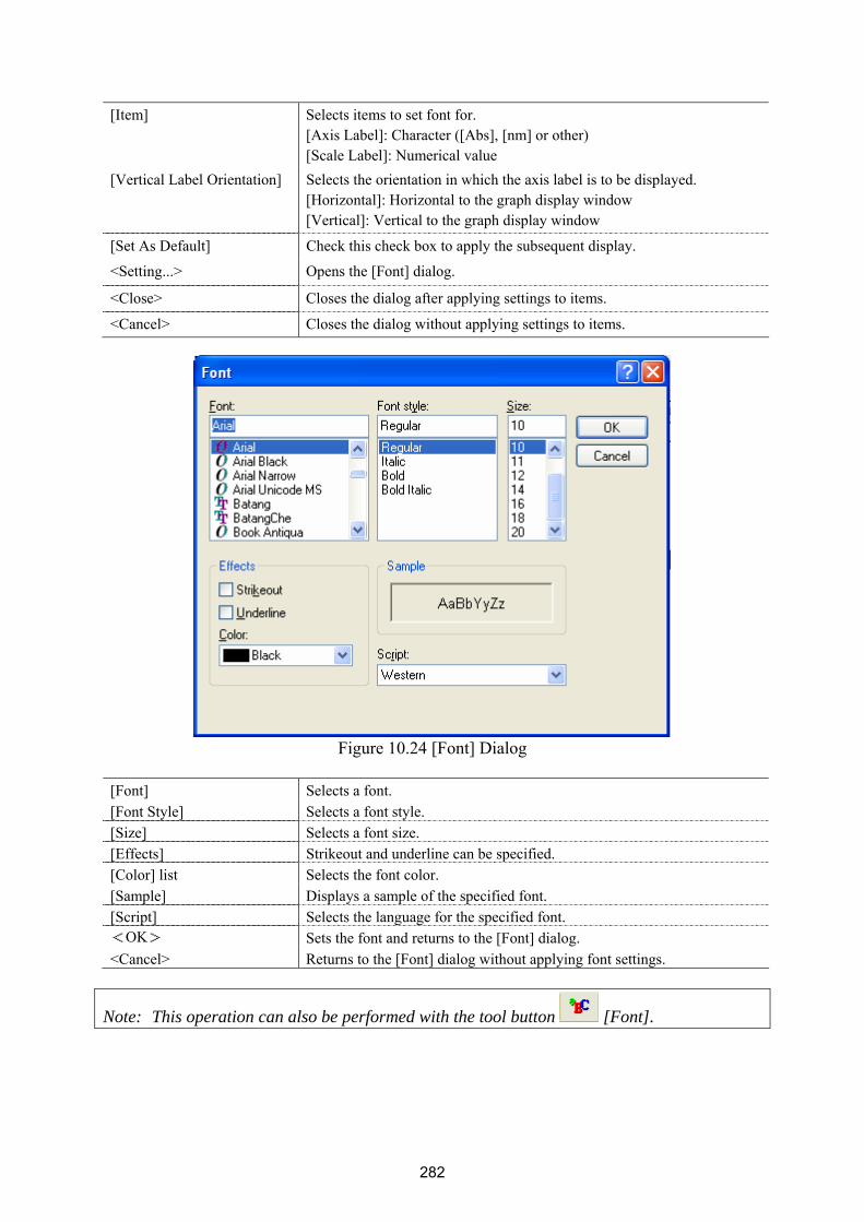
282

[Item] Selects items to set font for. [Axis Label]: Character ([Abs], [nm] or other) [Scale Label]: Numerical value

[Vertical Label Orientation] Selects the orientation in which the axis label is to be displayed. [Horizontal]: Horizontal to the graph display window [Vertical]: Vertical to the graph display window


<Setting...> Opens the [Font] dialog.




[Font] Selects a font. [Font Style] Selects a font style. [Size] Selects a font size. [Effects] Strikeout and underline can be specified. [Color] list Selects the font color. [Sample] Displays a sample of the specified font. [Script] Selects the language for the specified font. ＜OK＞ Sets the font and returns to the [Font] dialog. <Cancel> Returns to the [Font] dialog without applying font settings.

Note: This operation can also be performed with the tool button [Font].

283

10.3.2.4 [Gridlines…] Sets whether to show/hide of grid lines.



Note: This operation can also be performed with the tool button [Gridlines]. 10.3.2.5 [Style…] Sets the graph display style.


284

[Axis] Select the setting form of the vertical or horizontal axis. [Scale label] [Interval: Auto] Check this check box to set the scale display method “Automatic”. [Interval: Manual] Check this check box to arbitrarily set the scale display. In manually

setting, the intervals of the main and auxillary scale labels can also be set.[Decimal Point on Scale Label]


[Set as Default] Check this check box to apply the subsequent display.

Note: This operation can also be performed with the tool button [Style]. 10.3.3 [Decimal Point…] Sets the number of decimal places to display for the photometric value on the monitor bar and when the photometric value display field is in digital view mode.

Figure 10.27 [Decimal] Dialog


reference). [Format] Sets the number of decimal places to display for the items selected in the

[Item] list.

Note: This operation can also be performed with the tool button [Decimal Point].

285

10.3.4 [Tolerance Level…] When a tolerance level is set, the photometric value can easily be identified as lying within or outside of the tolerance level. If the values are within tolerance levels, the photometric value is displayed in green. If the values are outside of the tolerance level, the photometric value is displayed in red. If [Tolerance Level] is turned off, the photometric value is displayed in yellow. Note: Only available when the photometric value display field is in digital view mode.

Note: This operation can also be performed with the tool button [Tolerance].

Figure 10.28 Digital View Window

If the photometric value color is: Green: Within the tolerance level Red: Outside the tolerance level Yellow: No tolerance level is set.

286

Figure 10.29 [Tolerance Level] Dialog

[Enable Tolerance Level] Sets whether to use the [Tolerance Level] determination function. [Tolerance Level] Sets the tolerance level value. ≥ and ≤ □ A photometric value of □ and above, □ and below is the tolerance level.≤ □ A photometric value of □ and below is the tolerance level. ≥ □ A photometric value of □ and above is the tolerance level. < □ A photometric value of less than □ is the tolerance level. > □ A photometric value that is above □ is the tolerance level.

10.3.5 [Information Bar] Sets display/non-display of the information bar. 10.3.6 [Toolbar] Sets whether to display/hide the toolbar. [Measure] Shows/hides the toolbar corresponding to the [Measure] menu. [Control] Shows/hides the toolbar corresponding to the [Control] menu. [View] Shows/hides the toolbar corresponding to the [View] menu.

10.3.7 [Status Bar] Sets whether to show/hide the status bar.

287





Button Name

[Blank]

[Dark]

[Parameter]

[Preview]



Button Name

[Move Wavelength]

[Optical Path Check]

[Band Width]

[Response]

[Deuterium Lamp]

[Halogen Lamp]

[Auto Zero]



Button Name

[Analog Meter]

[Digital Meter]

[Graph]

288

[Scale]

[Pattern]

[Font]

[Gridlines]

[Style]

[Decimals]

[Tolerance Level]

[View Name] If this checkbox is checked, the button names are displayed under each

toolbar button. <Customize> Click this button to start up a dialog to customize the toolbar (see Fig.

10.31)


10.4 [Help] Menu 10.4.1 [About…] Displays version information for this Abs/%T meter measurement program.

289

JASCO Corporation 2967-5, Ishikawa-cho, Hachioji

TOKYO, JAPAN

Printed in Japan

v-600 operation - university of california, irvinedmitryf/manuals/v-670 user guide.pdf · i preface...

Documents