v'/ · modern control concepts with new identification techniques to develop a ... • a...

NASA-CR-201886

METHODS FOR IN-FLIGHT ROBUSTNESS EVALUATION

/V'/

SUMMARY OF RESEARCH

James D. Paduano Eric Feron

Department of Aeronautics and Astronautics

Massachusetts Institute of Technology, Cambridge, MA 02139

Marty Brenner

NASA Dryden Flight Research Center

MS 4840D/RC, Edwards, CA 93523-0273

1 INTRODUCTION

This is a report for the NASA Consortium Program NCC2-5116, entitled

'Methods for In-Flight Robustness Evaluation'. The goal of this program was to combine

modern control concepts with new identification techniques to develop a comprehensive

package for estimation of 'robust flutter boundaries' based on experimental data. The

goal was to use flight data, combined with a fundamental physical understanding of

flutter dynamics, to generate a prediction of flutter speed and an estimate of the accuracy

of the prediction.

This report is organized as follows: the specific contributions of this project will be listed

first. Then, the problem under study will be stated and the general approach will be

outlined. Third, the specific system under study (F-18 SRA) will be described and a

preliminary data analysis will be performed. Then, the various steps of the flutter

boundary determination will be outlined and applied to the F-18 SRA data and others.

2 SPECIFIC CONTRIBUTIONS

The specific contributions of this project include development of a robustness problem

formulation for flutter clearance, software development, and testing of general

identification methodologies on recorded flight data. The software developments include

• A new subspace identification algorithm that takes into account the presence of

multiple data sets,

This research was supported by NASA Ames University Consortium,Re: NCC2-5116.

https://ntrs.nasa.gov/search.jsp?R=19960041233 2018-07-18T03:35:32+00:00Z

• A novel algorithm to identify transfer functions in very noisy environments,

• An algorithm to identify a parametric model of flutter dynamics based on frequency

response using a Newton-based optimization procedure.

* A procedure to project validated models to a predicted flutter boundary, based on

modem robustness analysis methods.

• A first-cut demonstration of the flutter boundary prediction procedure for NASA

Langley wind tunnel flutter test data.

In addition to the demonstration on Langley data, all of these algorithms have been

tested on flight data provided by Dryden. Their validation is currently under study. The

contributions related to subspace identification have all been reported in a paper that

appeared at the AIAA Guidance, Navigation and Control Conference [1] and is provided

in an Appendix.

3 PROBLEM STATEMENT AND APPROACH

3.1 Problem Statement

Current flutter clearance procedures rely on post-processing of flight test data,

which significantly slows the envelope expansion process for new or modified aircraft. A

priori prediction of the flutter boundary is difficult, and flight test data axe currently not

used to systematically update these a priori predictions. Further, many methods for

determining proximity to the flutter boundary are based on either damping ratio

identification or tracking the evolution of spectral peaks. Experience and analysis have

shown that these measures can be highly nonlinear with respect to flight parameters such

as dynamic pressure and Mach number, and thus may be misleading measures of flutter

stability (we present a simple illustration of this problem below). A method is needed to

alleviate these difficulties, that systematically combines a priori knowledge on the

aircraft with flight test data into a well-behaved prediction of the flutter boundary, and

that does so in near real time so that envelope expansion can proceed more efficiently.

Current practice of using damping ratio as a measure of proximity to instability is

motivated by the fact that as an aeroelastic mode approaches neutral stability, its

damping ratio approaches zero. Thus one way to predict the flutter boundary is by

tracking the damping ratio of each flexible mode as a function of critical parameters

(dynamic pressure or Mach number), and subsequently predicting the flutter boundary by

2

simple linear extrapolation. In many cases however, such a measure can be unreliable.

For example, we have plotted in Fig. 1 the evolution of the damping ratio as a function of

speed for a typical wing section [8]. We see that a linear extrapolation of the damping

ratio will systematically overestimate the flutter boundary. Besides, when far away from

the flutter boundary, the damping ratio actually increases as the aircraft approaches

flutter.

Typi_ _ Se¢ t_ _o]_]e _,,

/.z.. OD2

o_1

ikh "_ 0

_. -oD4

D=,_i_g _ vers_sDee_ADo s_o,_ Lst_e 3re_inte_{0} ,_.rs_ _t_d IX] fl_er_o_

.o ....... o.o. ...... .oo.o.o.._o.oo.o.......moo...oo...o. o_o.oo..°oo o.-o_oo-o-.o oo° .....

! ! i i . .

i .

iiii i iiio o$ 1 15 2 25 3_0

no_ia_ ns_l wbcit_ fV/_c,:,]

Figure 1 - Evolution of damping ratio vs. speed for a typical section.

3.2 Approach

The approach proposed in this research may be sumarized in the following

diagram:

ICompac IPhYsic I I u r und ldata I datamodel I model I estimate I

Subspace 133 or Nonlinear Robustnessdirect TF estimation least-squares Analysis

To develop a reliable flutter clearance capability, we cast the flu tter clearance

problem as a 'robustness problem' typical in control applications. The flutter clearance

problem stated as a robustness problem is simply this: based on the currently available

3

dataandmodels,what is the 'smallest' perturbation to the current flight condition which

will drive it to the flutter boundary? Size of the flight condition perturbation is

represented as a norm or vectoral distance; this type of measure is typically much more

well-behaved than damping ratio or spectral peak amplitude. It is called the structured

singular value in control theory, and it is the multivariable counterpart of the classical

gain margin for single-input, single-output control systems. Several tools are now

available that compute it quickly and accurately.

To incorporate flight test data into the robustness problem, we take a unique

approach which involves compressing information from multiple data sets, taken at

various flight conditions. This is necessitated by the quantity and quality of the data

available (large amounts of relatively noisy data), as well as the nonlinearity of the

variation of the dynamics with flight condition. Model structure information is retained

by the procedure, through a nonlinear least-squares fit of the system dynamics to the

acquired data.

To 'compactify' the data and allow more efficient identification, subspace

identification methods have been investigated (see for instance De Moor and Vandewalle

[1] and Van Overschee and De Moor [2]). Alternatively, we also have investigated the

possibility of compressing data by directly generating reliable, de-noised transfer

functions. Both technique are essentially parameter-free identification procedures, which

provide models that are much reduced in size compared to the original time domain data,

but which are completely unstructured and therefore require additional identification to

be useful for robustness analysis. This additional identification is performed by adjusting

optimally the coefficients in an aeroelastic model that is known a priori, such that both

models agree as well as possible from an input-output viewpoint. Currently the

optimization criterion is a frequency weighted H2 norm.

4 SYSTEM DESCRIPTION AND PRELIMINARY DATA ANALYSIS

4.1 System description

The F-18 SRA (Systems Research Aircraft) is a test aircraft that has been equipped with

sophisticated flutter envelope clearance equipment, including a pair of aerodynamic

wingtip exciters that provide oscillatory wingtip lift. Ten accelerometers are located on

all the aircraft's body to measure the aeroelastic effects of the excitations. The table

below summarizes the numbering and position of each sensor.

4

Output12345

sensor location

left wing forwar(left wing aftlett aileron

left vertical tailleft horizontal tai

6 right vertical tail78910

right horizontal t_right wing torwar

right wing artright aileron

Accelerometer locations

The inputs were chosen to be sinusoidal sweeps spanning the 3-30I-tz range. This range

was chosen because it is expected to contain all the flutter modes for the F-18. The

sampling frequency was chosen to be 200Hz. Each sweep lasted 30 seconds to

compromise between the need for reliable information and the requirement to save on

fuel and maintenance costs.

To be sure to excite the symmetric and andsymrnetric dynamics of the aircraft, each test

consisted of two sequences. In the first sequence, the two exciters were roughly in phase,

whereas in the second experiment, these exciters were roughly 180 degrees out of phase.

The tests were performed at different elevations (10K, 30K and 40K feet) and different

Mach numbers (.8, .85, .9, .95) to obtain a broad range of flight conditions. The

operating conditions at which tests were performed is plotted on the graph below, along

with the aircraft flight envelope and the assumed flutter boundary.10 4 Flight envelope of the 1=18 and flight points wth data

' ............................. jl.......i4 ......... i .......... i ......... i .......... _ ....... _ .................................. : ......... i

• : : : : : : /

......... ::......... i .......... i .......... i ......... ! .......... _........ _........ ;,-_.......... :

:: i i i i i i," i

1 .......... _ .... _'__'i ..............

0 e" i

! : /, ! !

:15% flutter margin: i ,,.... :," ! i

I I I I I I I I

-10 0.2 0.4 0.6 0.8 1 1.2 1.4 1.6 1.8

Mach number

4.2 Data analysis

The data were collected from a real flight test and were significantly corrupted by

atmospheric and other disturbances. In addition, some sensors were suspected to be

defective. To investigate both issues, coherence plots between each input and each output

were computed. The corresponding coherence plots may are illustrated in the figure

below, which is based on a flight test performed at Mach 0.8 and 10K feet.

It may be immediately remarked that on average, the measured coherence is low

(no more than 0.8 in most cases). This indicates that the data at hand are contaminated by

high levels of noise. From experiment to experiment, the coherence was also found to

change significantly (possibly due to different weather conditions); such a difference in

coherence may be used to weight results from many experiments differently. To quantify

the results that have been obtained, a norm on the coherence plots was chosen to be the

mean of the coherence between 0 and 50Hz, bearing in mind that the excitation

frequency range is from 3 to 30 Hz. The resulting norms are tabulated below.

0.$

O,e

O.4

0.2

I_ %i2_uq)ul I

o.a

o,4

o.

0,3

0,2

O.

0 5O 100

_rmquency

irlp_ 2 oul_ 4

0_

0_

0 SO 10<)

6

_ 1 outmi S

0.4

0,1

00 5o 100

Irequ_of

0,4__

0.3

0.2

0.1

0

f_

0.4

0.3_

0.2

oo SO Ioo

fr_r_-y

t_o_ 2 output 6

0.4

0.3

0.2

O.

input 1 ouLp_ 70,4

0.2

0. I

00 5O I00

tlequo,_'y

P,pul 2 o¢4put 7

02

O.

•_ IO0 0 SO IO0

O.8

0.8

0.4

0.2

00 SO 100

hi,runty

i_ 2 o_puZ 8

0.8

0.8

0.4

0.2

00 5o lOO

fr_e.,e_-y

l_oul 1 o_p_ 9

0.8

06

04

O2

0o 5o IOO

Irequ_-y

input 2 ougpul 9I

0.6

11,4

O.

input I _JlpUl 10

0.8

0.6

0.4

O.

0 5o 10O

Irequqmcy

It*put 20ttlpul _0

0,8 _

02

00 50 100 0 50 100

f_ope('cy trequlmcf

Data output 1 output2 output30.359 0.33 c 0.190;0.415 0.426i 0.181_

," 0.289 0.267_ 0.155"= 0.241 0.200_ O.157_

0.463 0.455, 0.305"( 0.426, 0.428 c. 0.284C

0.399 0.39_ 0.230C0.34 0.3/4_ 0.219 _.

c 0.394 0.385C 0.248"1( 0.412 0.420, _ 0.257,1 0.366 0.368( 0.262,1; 0.441, 0.433._ 0.338_1C 0.379' 0.359_ 0.209(I_ 0.493 0.496 0.2811_: 0.360: 0.394_ 0.236_1_ 0.400 0.414i 0.212, _17 0.329: 0.296i 0.210',1E 0.379! 0.321 0.197_lC 0.3861 0.328_ 0.22_2C 0.147! 0.161: 0.354_

Average 0.371_ 0.363, 0.2341

output 4 output 5 output 6 output 7 output 8 output 9 output 1(0.11 0.106( 0.128. 0.111 _ 0.475_ 0.380, 0.382

0.206 0.124, 0.2221 0.139_ 0.4_ 0.371_ 0.3//:0.210 0.140_ 0.250: 0.132' 0.410 0.23z 0.276

0.1 { 0.103_ 0.132 0.108 0.286 0.227" 0.279:0.141 0.1_ 0.1831 0.130, = 0.496 0.542: 0.407_

0.187 0.17 0.2491 0.156{ 0.444 0.499, 0.321:0.21 0.142_ 0.237: 0.122,= 0.470: 0.520 _, 0.347,

0.26,.b_ 0.191 0.2_6 0.1 11 0.408 0.492( 0.2B3:0.204: O.133, 0.256: 0.123 0.473 0.471 _ 0.353:0.25! 0.13E 0.248; 0.118; 0.443 0.491 ( 0.31

0.101; 0.117, 0.093 0.115, 0.535 0.547, 0.505,0.173 0.169,' 0.199, 0.152" 0.456 0.487, 0.418,0.092: 0.102( 0.112_ 0.104,( 0.500' 0.461 _ 0.4300.19b: 0.146 _, 0.245! 0.139i 0.411 0.4,'.'.'_ 0.3990.235_ O.141 0.258, 0.137,= 0.404- 0.436: 0.3210.156: 0.140,= 0.21, 0.129 c, 0.42: 0.4971 0.320.143; 0.101 0.180! 0.09( 0.35_ 0.262, 0.3:0.276: 0.12E 0.273: 0.124 c. 0.315 0.252 (, 0.3040.270 O.152= 0.3011 O.138( 0.356 0.259_ 0.4080.199; 0.09_ 0.166: 0.108, 0.3/2 0.249 0.40b.0.190. 0.133_ 0.21: 0.1281 0.428 0.40; 0.359

Coherence with right input

Data output 1 output 21 0.520( 0.496!2 0.502_ 0.4u0,3 0.384 0.324

4 0.5091 0.404:5 0.602`= 0.6021

6 0.640 0.628:0.56, 0.556(

t 0.b47 0.536'( 0.554 0.532,

1( 0.551 0.5;1 0.642 0.649_1-" 0.662 0.695:1" 0.567 0.562lZ 0.536_ 0.5_

1,= 0.543, 0.5411E 0.539 0.5511_ 0.459 0.35_14 0.481: 0.356;1_ 0.4821 0.358=2_ 0.21 / 0.180_

Average 0.5241 0.496

,output 3 output 4 output 5 :output 6 output 7 output8 output9 output 100.221_ 0.115 0.101 0.142, 0.106! 0.382, 0.318: 0.316;0.215! 0.209 O.127 0.223 O.134l 0.434; 0.36, 0.364t0.179 0.219 0.142_ 0.245 0.133'. 0.3571 0.227_ 0.254, =0.266_ 0.212 0.1_ 0.251 0.128_ 0.20( 0.18" 0.18 <,0.381; 0.150 0.131 ! 0.193: 0.1 33! 0.452! 0.495: 0.37_0.382 0.21, 0.168: 0.254- 0.165! 0.389( 0.430_ 0.296"0.284 0.21 0.150 0.262: 0.128 0.402! 0.474 0.3410.285 0.255 0.1 _, 0.29, 0.179: 0.369: 0.418. 0.270=0.287_ 0.229 0.129, 0.293 0.132_ 0.402! 0.440: 0.349_,0.298_ 0.294 0.13_ 0.304_ 0,128: 0.422 c, 0.438 0.3160.434_ 0.104 0.115: 0.1" 0.1181 0.340: 0.336, 0.330 i0.527, 0.165 0.185! 0.226_ 0.134! 0.297, 0.328, 0.2710.271! 0.093 0.097! 0.1114 0.105! 0.393 c, 0.368 0.347_0.294; 0.195 0.14_! 0.235 0,131i 0.4,58,' 0.4_5_ 0.3910.2871 0.235 0.141 ! 0.288 0.136_ 0.358_ 0.390 0.3250.2811 0.158 _ 0.1391 0.239_ 0.134! 0.372; 0.434 0.306!

0.259( 0.149 _ 0.10; 0.184; 0.093, 0.313,' 0.253_ 0.318_0.22_ 0.27_ 0.1341 0.272q 0.131 0.284 C, 0.248_ 0.303

0.354! 0.269 _ 0.163, 0.279! 0.129! 0.293 0.237, 0.334,0.144_ 0.174 t 0.115, 0.1,54: 0.146[ 0.194_ 0.18,3! 0.199_:0.294, 0.197| 0.138" 0.228, 0.131: 0.355 c, 0.350: 0.310:_

Coherence with left input

Data flight# Mach altitude= input type

1 533 0.85 1 Ok symm2 533 0.85 1 OK asymm

3 533 0.9 10k symm

4 533 0.9 1 Ok asymm

5 531 0.85 30k symm

6 531 0.85 30k asymm

7 531 0.9 30k symm

8 b31 0.9 30K asymm

9 531 0.95 30k symm

10 531 0.95 30k asymm

11 532 0.7 10k symm

12 532 0.7 1Ok asymm

13 b32 U.8 10K symm14 532 0.8 10k asymm

15 532 0.95 30k symm

16 532 0.9 30k symm

17 533 0.95 10k symm

18 533 0.95 1 Ok asymm19 533 0.98 1Ok symm

20 533 0.98 10k asymm

Flight condition for each data set

The average of this norm for each outputs and for both inputs was calculated; it appears

that five outputs consistently have a much higher score than any other outputs. These five

outputs are the leading and trailing edge accelerators on each wing, and the right aileron

accelerator. It was decided to discard the latter, because it also measures the aileron's

8

own dynamics, which are neglected in the ensuing analysis. When more experience is

acquired, this viewpoint may be revised.

Browsing through the public domain literature has led to interesting comparisons. For

example, Bucharles, Cassa and Robertier [7] use signals with average coherences ranging

from 0.9 to 0.95 to perform the flutter analysis of Airbus commercial aircraft.

5 DATA COMPRESSION

Two data compression approaches have been investigated during this research. First,

subspace identification algorithms have been tested and improved. Second, because the

data under consideration are so noisy, an alternative direct transfer function evaluation

scheme was developed, which is robust to a large range of noise disturbances.

5.1 Subspace identification: review of existing techniques and new developments.

As most of the information gathered during this phase of the project has been already

reported in the conference paper [1], this section will only highlight its main f'mdings.

The attached appendix contains the conference paper.

Subspace identification techniques represent a way to perform system identification in an

unstructured way, using state-of-the-art results in matrix computations, including least-

squares and total least-squares techniques. Subspace identification techniques are

essentially "black-box" algorithms, which attempt to infer a low-order, state-space

model that "best" explains a given set of inputs and outputs. To evaluate how useful

these procedures are for aerospace applications such as flutter boundary determination,

the F-18 SRA data were used as benchmark data. Many subspace algorithms currently

available were tested on these data, especially the algorithms by Cho and also by

DeMoor [1]and VanOverschee [2].

The results of this study led to the following conclusions:

(i) The collected data are often distributed over many flights at the same flight condition.

This is incompatible with existing subspace identification software, which were all built

for single I/O data sequences. To remedy this problem, the basic principles of subspace

identification were reviewed and adapted to handle many, uncorrelated data sets. This

technique has since then found applications in other areas of interest to NASA-Dryden,

including thereliableidentificationof theF-18SRA lateral-directionaldynamicsfor

nonlinearsimulationcalibrationandautopilotdesignpurposes.

(ii) Thedataareverynoisyandsubspaceidentificationmethodsareon thewholeunableto copewith theselevelsof noise.Besides,different subspaceidentificationtechniques

donotall sharethesameperformance.As aresult,analternatedatacompressionscheme

wherebytransferfunctionsaredirectly estimatedhasbeendevised.

5.2 Direct transfer function estimation

This method is based on the a priori knowledge that the input signal is a frequency

sweep. Thus it is possible to predict a priori at what time the relevant frequencies should

appear in the input and output signals.

5.2.1 Single input-single output case

We first consider the single input-single output case. The assumptions for this method is

that the excitation is a frequency sweep. Process and observation noises are present as

shown in the following figure.

__Input

noise

Inputsignal

SystemG(jo )

IOutput

I "_" Outputsignal

The step by step procedure of the transfer function estimation is described as follow.

Step 1: localization of the relevant frequencies by filtering the signal with a set of narrow

band pass f'flter centered around the frequencies _,. Filtering the input and the output

does not alter the identification. Indeed if the input and the output of the system are

f'fltered with the same linear time invariant filter F, the filtered output appears as the

output of the system excited by the filtered input.

10

Step 2: localization of the relevant time information by windowing each f'Lltered signals.

The chosen window has to be the same for the input and the output and is chosen to be

centered at the point where the FLltered input has the maximum amplitude. At this step,

the two signals should appear as sine functions.

Step 3: calculation of the estimate at the frequency (°l by the ratio of the output Fourier

transform of the windowed signal to the input one:

Ym°st"lu Yme_nd _esdenotes the measured signals.8(jo ,)= u..,(n)e ' where

Let us now look at the properties of this estimate. Let r_ and rh be the input and output

noises, respectively. Then we have

8(j(oi ) = G(j_i )( Y[ j_i) + NI( J(°i)) + Nz( j_i)U( jo_,)

N,(j_;) N2(jo_,)

= G(./Lo,)+ G(j_,)U(j_,) + U(j_,)

If the two noises are assumed to be unbiased, then _(J°3i)=_-_Tli(k)e-_i_k=O

Therefore, _(jc.oi) = G(jo3i), i.e. the estimate is unbiased.

_N 2= E(_-_ n(k)2) = N°G2 where O2is theThe variance of the noise is given by

variance of the noise, and N° is the number of points in the time window. The variance

of the transfer function estimate can now be calculated, assuming that the two noises are

uncorrelated:

,U(j_,)=---_U

Assuming that the windowed input is a sine function,

amplitude of the input, the variance of the estimate is

4°12 +-_2=lG(jo,,)i2

, with U being the

5.2.2 Multiple input single output case

At this point, let us assumed that the system has m inputs. A set of m independent

experiments is necessary to use the proposed method and all the excitations are assumed

to be frequency sweeps. The first step is identical to the single input case. The property

11

that thefiltered output will be identical to the output associated with the filtered inputs is

still satisfied since, in the Fourier domain, the matrix of the filter is a scalar matrix which

commutes with any other matrix. For the second step, the procedure is the same but one

of the m inputs has to be taken as a reference in order to select the time window. For the

third step, the Fourier transform of every signal has to be calculated and the estimate is

given by

(%(jo_,)j Lu.,(_,)... u_u_,)j LY_(joJ,)jwith Uk, the 1_ input of the k" experiment. Note that the input matrix has to be full rank

in order to apply this formula (if it is not full rank, we conclude that t here not enough

information in the data to estimate the transfer function). With the same assumption for

the noise, the estimate still has no bias. The variance of the estimate is given by

&(#')-_(#') l[c.(j_,) _(j_,)o'_=E

G_ (jo_,)

where E stands for the expected value.

becomes

... ¢'(jo,,)-_(j_.)}

By plugging in the value of the estimate, this

r U,, (jm;) -.-2 ;

°_ LU_(jm,) ...

[ _._pGp(jo_,)N_p, (j_,)+ N_,

Lu_ (jo_,) ... U,,_(j_,)J

Since all the noises are assumed independent, this equation becomes

12

[ U,,(ko,)O G =

i L,.,,,,r_,_

_IG,,IJ'o,o

• .. Ulm (J(,Ol): ]1

... U% (jo_/)

n 2 2InPl D "J" No_ID

0

... 1-

... ,.,,,,.iJo,,__l

o o 1• Io. ,...0 Gp(jO_) N_,_2+ No,_,o

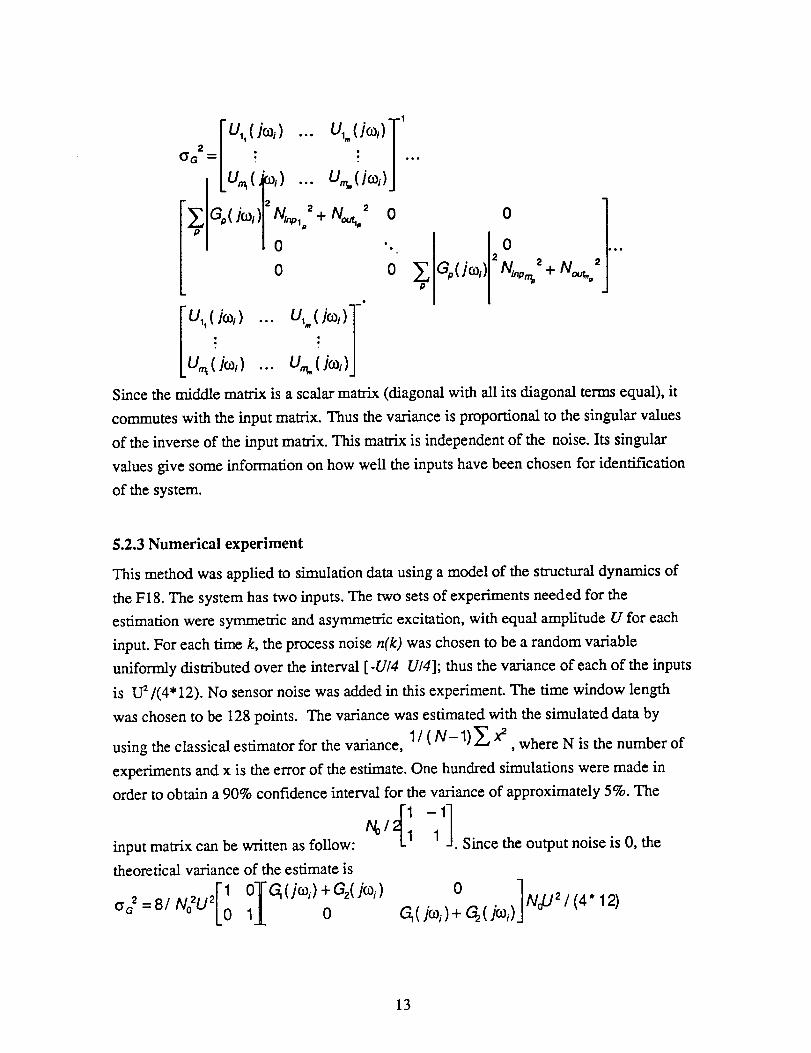
Since the middle matrix is a scalar matrix (diagonal with all its diagonal terms equal), it

commutes with the input matrix. Thus the variance is proportional to the singular values

of the inverse of the input matrix. This matrix is independent of the noise. Its singular

values give some information on how well the inputs have been chosen for identification

of the system.

5.2.3 Numerical experiment

This method was applied to simulation data using a model of the structural dynamics of

the F18. The system has two inputs. The two sets of experiments needed for the

estimation were symmetric and asymmetric excitation, with equal amplitude U for each

input. For each time k, the process noise n(k) was chosen to be a random variable

uniformly distributed over the interval [-U/4 U/4]; thus the variance of each of the inputs

is U 2/(4"12). No sensor noise was added in this experiment. The time window length

was chosen to be 128 points. The variance was estimated with the simulated data by

using the classical estimator for the variance, 1 / ( N- 1) _ x 2 ' where N is the number of

experiments and x is the error of the estimate. One hundred simulations were made in

order to obtain a 90% confidence interval for the variance of approximately 5%. The

input matrix can be written as follow: . Since the output noise is O, the

theoretical variance of the estimate is

13

= i / 3NoI (jco,)+6 (jco,) 0 10 _(jco,)+G2(jo),)

Note the variance of the transfer function estimate is independent of the noise amplitude.

The variance was compared with the theoretical results and plotted below. In this case,

the standard deviation of the variance estimate is 5% of the estimate and is independent

of the freauencv.Irma_l_er _tlrC|_ e_l_Io vlf_nCe _ II_i IfAnllor ru_¢llo_ _llmnle

2_

. I I ,1_ t tl

jl

0 5 I0 15 20 25

fr_ta_mcy (in HZl

_ioUd line - estimated transfer function

Dashed line - actual transfer function

°[t400 "

1200

30 tO00

O00

600

4O0

2O0

030

_ . J.., '_5 10 15 20 25

frequet_-f (_ Hz)

Solid line - theoretical variance

Dashed line - estimated variance

30

5.2.4 Application to F18-SRA data

This method was then applied on the real flight data using only the four outputs chosen

in Section 2. The four transfer functions plotted below were obtained from F-18 SRA

flight data taken at 10,000 feet and Mach 0.8. The f'trst transfer function (input 1 to

output 1) starts with a slope of 40 dB/decade at low frequency and a phase of 180

degrees. The phase then drops to -360 degrees and the magnitude is constant, at around

40 dB. This means that there is a second order pole at 6.5 Hz. It seems that there is also a

pole zero cancellation around 13 Hz. However, due to the low resolution of the estimate,

this cannot be aff'Lrmed by this plot only. The high frequencies (above 18 Hz) are rather

noisy, but it seems that the magnitude and the phase are stable, meaning no pole or zeros

are in this region. Looking at the second transfer function (input 1 to output 2), it seems

that the low frequencies have the same properties as the In'st plot which is a slope of +40

dB/decade for the magnitude with a phase of +180 (which is the same as -180). The pole

at 6.5 Hz is still detectable on this plot and a pole around 12 Hz is also seen. This

conf'm'ns the pole zero cancellation of the previous plot. For the asymmetric excitation,

two poles could be detected by looking at the magnitude of the transfer function at 8 and

14

18 I-Iz. However, it is much harder to correlate the phasein this case,becauseits

variationwith frequencyismuchsmoother.

Input i =-) Output I

i.., i i .... i.......

io'

r _ : _.i.: ii .............

)o'

_On Ml)

Input 2 --) Output I.ira

_. •

io'

w_ fl_ I,tll

Input I "=) Output 2

_--_ .... i....... i........ i _ ...............

i_.Iii̧iiii:iiliiiiii̧ii!,iiiiiii_)o (

lrm_incy On )_)

Input2 --) Output 2

=mlI0'

_00 .... ,

)o'

6 IDENTIFICATION OF STATE-SPACE DYNAMICS BASED ON COMPRESSED DATA

Once the data are compactified (either in state-space via subspace identification or via

direct transfer function estimation), it is necessary to fit a physical model of the system to

them,

where the input/output form of this model is given by

X= AX+ BU

Y= CX+ DU

The parameters in the fitting procedure are the significant elements of the system

matrices (A, B, C, and D), where the system states are the physical states, and the initial

guess and structure of the model (structure is represented by the zero and identity

15

Techniquesfor Flutter Clearance September25, 1995

elementsof thesystemmatrices)comefrom a priori modeling. In its basic version, the

fitting operation consists of minimizing the H2 norm of the difference between the

system deemed by the matrices (A, B, C, and D) over the relevant coefficients (such as

stability derivatives and aerodynamic lags) and the experimental, compressed data. In a

more sophisticated version, a series of fits is done f'n'st over a range of flight conditions.

These fits are then interpolated using a specific parameterization with respect to, for

example, Mach number and dynamic pressure q.

6.1 Nonlinear fit via Newton algorithm

To f'md a system of the form (1) that best matches the experimental data, we propose to

constraint some elements of the matrices to be constant in accordance to the nominal

flutter model that was chosen. The chosen cost function is the H2 norm of the difference

between the estimated transfer function and the transfer function of the identified model.

Even though some elements of the matrices were timed, the optimization problem is still

unconstrained in the mathematical sense since all the coefficients that are allowed to vary

are totally free.

The H2 norm for a system is given by:

J= I Tr(( C(jo)- A)-' B+ D- G( je ))( C(jo)- A)-' B+ D- G(/m))')ctt)0

The gradient of J with respect to all the matrices needs to be evaluated. With respect to

the matrix A, the gradient is:

_J

o_-._= 2 R e ( I Tr( (C ( j o_- A) - _dA( jo3 - A) - ' B) ( C( jo.) - A )- ' B + D - G( jm ) ) ") cto )0

By using the multiplication commutation inside the trace operator, we have

-.-:o_A=2_JRe(I Tr(((jo_ - A)-_ B)(C(jco- A)-_ B+D - G(jo3))" C(jo3 - A)-'dA)cto)0

With the same procedure, the gradient with respect to B, C and D can be evaluated:

_)J Re(f Tr( C( - A)-' B+ D-oa--_= 2 jo_ G(jo_))" C( jo3 - A)-' dB) cto) ,0

Oj *"- 2 Re(I Tr(( jo3 - A)-' B(C( jm - A)-' B+ D- G( ](o ))" dC)cto ), and

aa -2Re(I rr((ct]m- A)-' U+ O-OD

0

16


Theseintegralsarewell approximatedby a discretization(in frequency)at all thepointsat which the transferfunction hasbeenestimated.Thegradientof thefunction J canthenbederivedfrom theaboveformulas.

For a Newton optimization, it is also necessaryto calculated the Hessian H of the

function. However, this operation is computationally very intensive; it is generally more

efficient to use a so-called quasi-Newton method instead. This method estimates H based

on the variation of the value of the function and of the gradient. A efficient method to

estimate H is the BFGS method. Once H is estimated, the direction of search is

calculated by d= H-1VJ. An optimization of J along this search direction is then

performed to find the minimum J in the current search direction (i.e. the step length is

optimized). The classical 1D Newton method can be used at this stage, but it is then

necessary to calculate the derivative in the direction of search at each step. Studies on

optimization have shown that it is not necessary to f'md a very accurate minimum in the

current search direction because, at the next iteration, the direction of search is going to

change. The little gain obtained by optimizing in each search direction can usually be

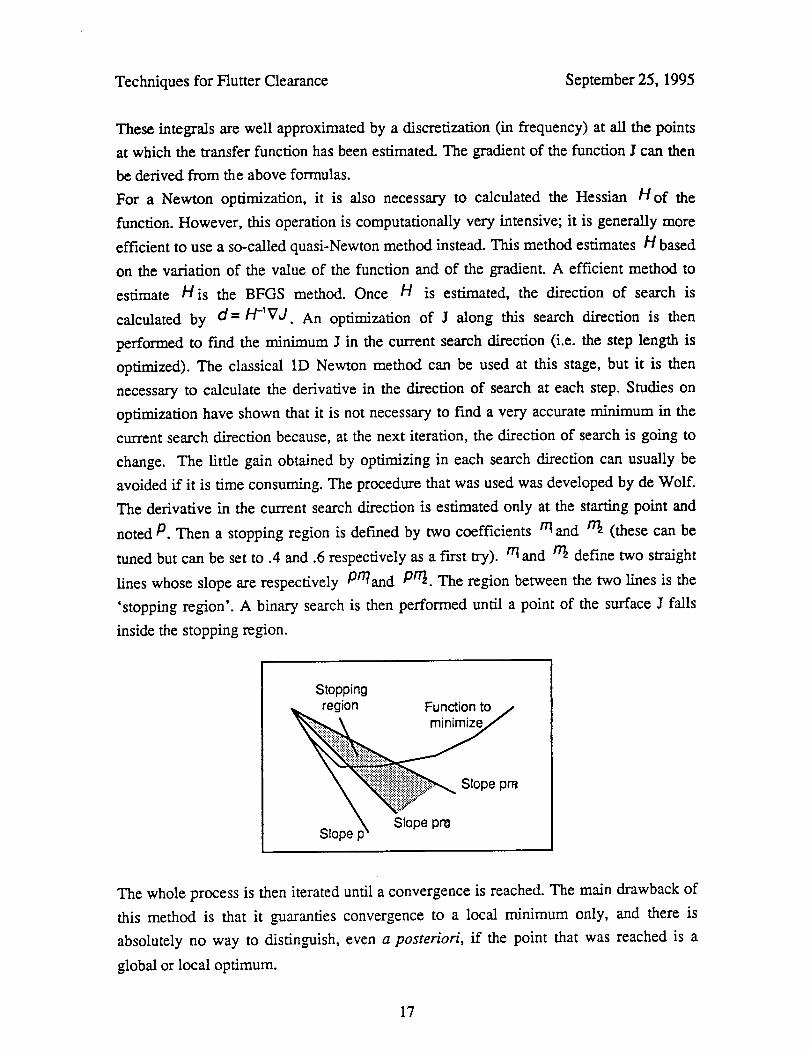
avoided if it is time consuming. The procedure that was used was developed by de Wolf.

The derivative in the current search direction is estimated only at the starting point and

noted P. Then a stopping region is defined by two coefficients _ and rr_ (these can be

tuned but can be set to .4 and .6 respectively as a first try). rrl and rr_ define two straight

lines whose slope are respectively prqand P_. The region between the two lines is the

'stopping region'. A binary search is then performed until a point of the surface J falls

inside the stopping region.

Stopping

region Function to j

\ Slope pr_Slope p,

The whole process is then iterated until a convergence is reached. The main drawback of

this method is that it guaranties convergence to a local minimum only, and there is

absolutely no way to distinguish, even a posteriori, if the point that was reached is a

global or local optimum.

17


6.2 Application to F-18 SRA data

6.2.1 Physical flutter model

The f'trst step to use the quasi Newton algorithm is to determine which elements in the

state space model are fLxed and which are to be optimized. Even though numerous flutter

models have been proposed, a literature search showed that the most common is written

as follows:

0 I 0A= -M-IK -M-tO -M-IF

0 0 A

where I is the identity matrix. The matrices M, K and C are the apparent structural mass

stiffness and damping of the aircraft which means that that the non-circulatory part of the

aerodynamics is included in the matrices. The lower-right matrix A represents the

aerodynamic lags and is a diagonal matrix with real negative eigenvalues. P is the

coupling term between the lags and the structure.

6.2.2 Actual data and high-order model

A f'mite element study of the structural dynamics of the F18 was computed by NASA

Dryden. The full model was composed of 14 symmetric modes and 14 anti symmetric

modes. 13 of them were in the 3-20Hz range and 11 of them may be involved in the

flutter mechanism. It was therefore decided to reduce the model to 11 modes (or 22

states). The first experiment that was tried was to put all the uncertainty into the lags.

The matrices M, K and C were set by reducing the theoretical model to keep only the 22

states of interest. For this, the state space system was diagonalized and only the modes

with the appropriate eigenvalues were kept reduced. The matrices P and A could vary in

the optimization and D was set to 0. It was assumed that the actuator acted as a force

input on the structure and did not affect the aerodynamics around the wing. Therefore,

the structure of the matrix B is chosen to be . The sensors are assumed to

measure only structural displacements and no aerodynamics at all. In the model this

shows in a matrix C of the form: C= [_ _ 0]. Finally, it was found to be necessary

to add an additional constraint in the Newton algorithm that forced the lag coefficients to

stay above a certain limit (so that the identified model remains stable).

18

Techniquesfor FlutterClearance September25, 1995

The optimizationsetup asdescribedabovesaturatestheconstraintson thelags,anddoes

not convergeto evena local minimum. Thus it wasdecidedto optimizeover a single

output,2 outputs,and 3 outputs,to determinethe effect of trying to fit more andmore

outputson theoptimizationprocess. First, only one outputwasusedandthe algorithmran with exactly the samestructureof matrices.A stablelocal minimum which did notsaturatethe constraintswas found for this case.A measureof the accuracyof theidentificationwasdefinedto be theratiobetweenthevalueof thecostfunction J andthe

nominalH2 normof theestimatedtransferfunction, evaluatedin %. This measurewent

downto 13.3%for thesingle-outputtest.Whena secondoutputwasadded,the accuracy

of the identified modeldegradedto 20.6%.Whena third outputwasadded,the accuracyof the identified modelstalledat 31.1%. Thuswe concludethat it is progressivelymore

difficult to explain all of thedatawith the singlemodel that weareusing; whenall four

outputsarechosenthesearchfails altogether.At thispoint, theorderof thesystemto be identifiedwasfurtherreducedto 6 modes.

Two thingsmotivatedthis approach.First,computationtime growsexponentiallywith

both thenumberof parametersto fit and the order of the system, since it is necessary to

calculate the inverse of a complex matrix of the size of A at every iteration. The second

motivation was to detect whether some of the modes in the models were absolutely

necessary. In this test, the system was modeled with only 6 modes. This approach

converged with all four outputs, and yielded a system of order 18. The solution found

had an accuracy of 33%. The figure on the following page shows the frequency domain

plots of all 8 transfer functions, together with the results of the optimization. Despite the

large value of the optimality measure, the basic shapes of the transfer functions have

been captured consistently across all eight transfer functions.

Based on these tests, we conclude that by reducing the model order, the difficulties

encountered with convergence were alleviated to a sufficient degree that the four-output

test was able to converge. The trend of error in the fit continues as expected, however:.

the percent error is highest for the four-output identification. It is important to note,

however, that the reduction in the model order did not significantly effect the overall

accuracy of the fit (31% vs. 33%). Thus the hypothesis that some of the structural modes

are indeed unnecessary to explain the data appears to be a valid one. Follow-on work is

focusing on judicious model order reduction, as well as optimization of the mode shape

parameters (contained in the C matrix) separately from the lag parameters.

19


J_p I--) Ott 1 _'_ip 2--) O,t,dIInip I _> oot 2 _p 2--) _ 2

: o.o_.................... o._ ......... :...............

o.o,5..... _....... ! .... o.0, ...... ......... ]°0" ...... .......: °.o,........................o._.......... . _o.o,

o _o.o .... °.°,!

° ! '........_'_......!..... ...... _ o1= .... .........I ° .... :..... ÷-=

..............r'zl 1 _0 lo 2o _0 0 lo 20 30 o _0 _ 3o --400 lo 20 3o

frequency _ HZ) fr_*_cy ('in HZ) fflquency [in HZ) frequency (in HZ]

k_ 1--_, out 3

0.03 -- . :

o.o2s_ t _i..........

zo.o,_.I._ ....: ........0.305/ j,_

o;- _o -_ 3o

hp 2--_ out 3 _p 1--> O*Jt4

°°1 t °'to.oas ........... i ....... o.os....... :. .... : .........

t °.02 ........ ! ...... _0._,......... i............

.....,..............!oino 2--> out 4

0,025

_ 0.02

_o,o,5I

0.01!

0.305 ........ i ........

1 t t' .̧........0 I0 20 30 -200_ 10 20 30

frequency {_ HI) Irequency {'in HI) ftequmncy (in HZ) frequency (in HI)

6.2.3 Simulated data and low-order model

Based on the results of the previous section, a test was executed using simulated data and

a very low order system. As before this was motivated by the desire to reduce

computation; for a very low order representation the number of local optimum should

also be reduced. Therefore, since the Newton algorithm converges to any local minimum,

the chances that the global minimum is reached are increasing. At this point, the physical

model that was used primarily was totally ignored. The number of modes was set to two

because two resonance appeared clearly on the transfer function estimates. The initial

guess for the A matrix was of the following form:

0 0 _A= 0 -q

-/£ q_

kz and kz were set so that their square root is equal to the approximate value that was read

on the transfer function plot. The values of c were set so that the system is stable. These

values were also chosen rather small since it is weU known that structural dynamics

20


eigenvaluesarelightly damped.Thenumberof outputswasreducedto two becausethe

symmetric and anti-symmetricpart were assumedto be completely decoupled.Theconvergenceof theNewtonalgorithmwasquite fastasexpected. More importantly, the

fits were acceptable(less than 10% of relative error, seecomparisonsbelow), even

thoughthemodelusedfor simulationhad14modesandthemodelusedfor identification

hadonly two modes.The experimentwas testedfor threedifferent altitudes(10K, 30Kand40K feet) andthe Machnumberwaskept constantat .8. At every flight point, both

the symmetricand anti symmetriccaseswere tested.The resultsof the identification

werealwaysgoodandtheconvergencefast if areasonableinitial guesswasutilized.

_Xo I --> oul 1

0 S 10 15 20 25 3O

At this point, even if we assume that the optimum that was found was the global

minimum, there is no guaranty that the three models are in the same basis. Therefore,

some additional constraints were added to the second and third identification, forcing

them to have the same C matrix as in the Fn'st identification.

Another experiment was tried with the same set of data and the same parameterized

model which consist in identifying the three Taylor expansion matrices in one single

Newton algorithm. Since only three flight points were considered, the Taylor expansion

should exactly match the previous results at the three elevations that were considered.

The initial guess for this experiment was taken as the result of the previous Newton

optimization for the nominal point, and the two other matrices of the Taylor expansion

were set to 0. This means that the initial guess assume a constant A matrix with respect to

the parameter.

21


6.2.4 Conclusions about F-18 SRA model identification

Several critical issues were identified for the success of applying the Newton algorithm

to identification of the structural dynamics of the F18. The computation time involved to

solve the problem can be quite high if the model order and number of free parameters is

not carefully considered. Choosing a reliable model order is a critical step, and further

work is needed to determine what constraints should be applied and how knowledge of

the physical system can be incorporated. Finally, the coefficients of the matrices should

not be completely independent; at the very least they should be tied to dynamic pressure

in a physically meaningful way - this is the focus of current research.

6.3 Analysis of the Benchmark Active Control Technology (BACT) Demonstrator at

NASA Langley

Initial development of procedures for flutter boundary prediction were also tested

in cooperation with NASA Langley, utilizing data from the BACT rig. This rig is a 32"

wing section mounted in Langley's transonic wind tunnel facility [3]. The purpose of the

device is to test flutter control strategies in a benchmark environment. Because of this

role, high frequency forcing can be introduced via trailing edge flaps and upper and

lower surface spoilers. Spectral transfer function estimates of the aeroelastic behavior

have been obtained, and detailed modeling has been conducted. Again, a nominal, finite

element model of this system was available to be fit with these experimental, compact

data, and we used the same Newton procedure to match this model with these data. In

this case, a series of fits was done fin:st over a range of flight conditions. These fits were

then interpolated using a specific parameterization with respect to, for example, Mach

number and q. The parameterization in use in this case is a quadratic of the form

A = Aq2q 2 + Aqlq + AM2M 2 + AMIM + AMqMq + A0. (*)

22


M,odol ] b'lt_lor Boundary

2OO

180 .... ! .................... i ...........

12'00.65 0.7 0.75 0.0 085. 0.9 0.95

Ma_ Numt)_

Me_,ure o/the Accuracy o/Predicted FlurrY" Dynamic Prl_c_rll [q)

1.1 • ,

"i, ' .... 0.gS

06 075 08 085 090.G5 0,7

Noenir_l tosl q / Actual flullo¢ q

Experimental (curved line) and predicted (x's) flutter boundaries for BACT using

approximate aeroelastic model and experimental frequency-response data. Circles in

plot at right correspond to flutter points (x's) on plot at left.

Typically, the matrices in the summation have the same structure as the original

aeroelastic model. However, the parameterization in Mach number and q does not

necessarily reflect the one originally present in the aeroelastic model. Rather, it is to be

seen as a low-order approximation of it, which is flexible enough to incorporate badly

modeled parameter dependencies such as Mach number.

The plots above show the results obtained by applying this procedure to the

Langley BACT data. The results are shown both on an M-q plane, and in terms of

percent prediction accuracy. The latter plot requires some explanation. If the procedure

is used during flight test, its accuracy becomes more important as the flight condition

approaches the flutter boundary. Because the prediction is projecting to a boundary

which is not as far away, the prediction also becomes more accurate as the flight

condition approaches the flutter boundary. At any flight condition, as a minimum, the

algorithm must say that it is safe to fly 50% of the remaining distance to the boundary. If

it does not, then the envelope expansion will be halted prematurely. Overprediction of

the flutter boundary may be acceptable when one is far from that boundary, but as it is

approached the prediction must become more accurate.

These considerations lead to the plot at left - if the predicted flutter speed falls

within the shaded region at all times, then the prediction is considered to meet the

minimum requirement for usefulness during envelope expansion. For the BACT it is

seen that we are very nearly successful based on only 6 data sets (this is the minimum

23


number of data sets necessary to eventually find a parameterization of the form (*)). It

remains to be seen if this accuracy can be obtained for data from a real aircraft.

Furthermore, since in the real case the flutter boundary will not be known, some measure

of the accuracy of the prediction must be developed.

7 REMAINING RESEARCH ISSUES

Our attempts at developing the methodologies outlined above have raised the

following issues:

• As compared to the BACT data used at Langley, the F-18 SRA data is more

complete; however it is corrupted by higher noise levels. As a consequence,

existing subspace identification procedures have difficulty providing accurate,

compact representations of the data. Improving identification accuracy will

require research on modifications to subspace identification methods (for

instance, frequency-dependent weighting). The relationship between the

efficiency of the subspace identification procedure and the excitation signal at the

wing tips is also an open research question. Discussions with members of the

Structures group at Dryden suggest that some alternate excitation schemes might

be implementable on existing hardware (currently logarithmic and linear sine

sweeps are used).

• The current nonlinear least-squares procedure to match the aeroelastic model with

the 'compactified' data is computationally greedy, although specialized time-

saving concepts such as Quasi-Newton have been used. While the size of the

Langley system allowed the procedure to converge acceptably fast, improvements

still need to be made for the same procedure to work on F-18 SRA aeroelastic

models.

• The choice of an appropriate parameterization as a function of Mach number and

q is still not clearly defined. The parameterization (*) is such that after optimal

fitting, some entries in the matrices Aq2, Aql, AM2, AMI, AMq or Ao may not be

physical (in other words, the aeroelastic model, if used alone, would predict such

entries to be zero). Schemes that impose the structure of the aeroelastic are

possible; however, the 'unstructured' approach allows one to correct for badly

modeled parameters such as Mach number.

• In order to convert the flutter boundary problem into a robustness problem,

various levels of sophistication are possible: in the most basic version, only the

24


Mach and q parametersappearin the perturbationblock A. However, one can

imagine that in the future, the two aforementioned steps (data compactification

and least-squares model matching) provide parameterized models with error

bounds; these could be easily and effectively inserted in the robusmess problem

as true additional uncertainties, leading to a more reliable analysis without

necessarily introducing unwarranted conservatism.

In order to make the tools usable during flight test, a significant decrease in the

computation time is required. Once methods with desirable properties have been

validated, optimization of the computations must be considered. Recursive

implementation, for instance, should be investigated.

An ongoing concern is proper interfacing of the proposed tool with the flight test

engineer. In particular, we will need to carefully examine how data pertaining to

flutter proximity should be displayed and documented in a reliable fashion. Also,

any procedure able to detect malfunction of the proposed method (for example,

bad fit of the experimental data) should be implemented and displayed as a

warning to the operator.

REFERENCES

De Moor, B., Vandewalle, J., "A geometrical strategy for the identification of

state space models of linear multivariable systems with singular value

decomposition," Proc. 3rd Int. Symp. on Applications of Multivariable System

Techniques, p. 59-69, Plymouth, UK, April 13-15, 1987.

2. Van Overschee, P., and De Moor, B., "A Unifying Theorem for Three Subsapce

System Identification Algorithms," ESAT-SISTA Report 1993-50-I, Department

of Electrical Engineering, Katholieke Universiteit Leuven, September 1994 (to

appear in Automatica).

3. Durham, M. H., Keller, D. F., Bennett, R. M., and Wieseman, C. D., "A status

report on a model for benchmark active controls testing," AIAA 91-1011, 32nd

Structures, Structural Dynamics, and Materials Conference, Baltimore, MD, April

1991.

4. Gondoly, K., "Application of Advanced Robustness Analysis to Experimental

Flutter," M.S. Thesis, Massachusetts Institute of Technology, June 1995.

25


. Miotto, P., and Paduano, J. D., "Application of Real Structured Singular Values

to Flight Control Law Validation Issues," AIAA Guidance, Navigation, and

Control Conference, Baltimore, August 1995.

o Duchesne, L, Feron, E., Paduano, J. D., and Brenner, M.,"Subspace

identification with multiple data sets", 1996 AIAA Guidance, Navigation and

Control Conference.

. Bucharles, A., Cassa, H. and Roubertier, J., "Advanced parameter identification

techniques for near real time flight flutter test analysis". AIAA-90-1275-CP,

1986.

8. Bryson, A. E., "Control of Spacecraft and Aircraft", Princeton University Press,

1994.

26

v'/ · modern control concepts with new identification techniques to develop a ... • a...

Documents