v. simoncini - dipartimento di matematicasimoncin/prec09.pdf · spectral analysis of saddle point...
TRANSCRIPT

Spectral analysis of saddle point matrices
with indefinite leading blocks
V. Simoncini
Dipartimento di Matematica, Universita di Bologna
Partially joint work with Nick Gould, RAL
1
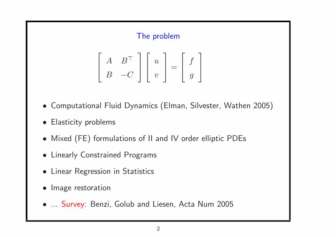
The problem
A B⊤
B −C
u
v
=
f
g
• Computational Fluid Dynamics (Elman, Silvester, Wathen 2005)
• Elasticity problems
• Mixed (FE) formulations of II and IV order elliptic PDEs
• Linearly Constrained Programs
• Linear Regression in Statistics
• Image restoration
• ... Survey: Benzi, Golub and Liesen, Acta Num 2005
2
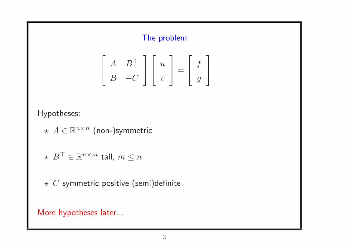
The problem
A B⊤
B −C
u
v
=
f
g
Hypotheses:
⋆ A ∈ Rn×n (non-)symmetric
⋆ B⊤ ∈ Rn×m tall, m ≤ n
⋆ C symmetric positive (semi)definite
More hypotheses later...
3

Why are we interested in spectral bounds?
• To detect “sensitive” blocks in the coeff. matrix
(guidelines for preconditioning strategies)
To “tune” the regularization parameter (matrix C)
To predict convergence behavior of the iterative solver
4

Why are we interested in spectral bounds?
• To detect “sensitive” blocks in the coeff. matrix
(guidelines for preconditioning strategies)
• To “tune” the stabilization parameter (matrix C)
To predict convergence behavior of the iterative solver
5

Why are we interested in spectral bounds?
• To detect “sensitive” blocks in the coeff. matrix
(guidelines for preconditioning strategies)
• To “tune” the stabilization parameter (matrix C)
• To predict convergence behavior of the iterative solver
6

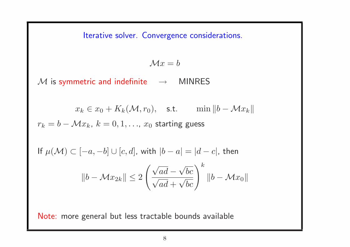
Iterative solver. Convergence considerations.
Mx = b
M is symmetric and indefinite → MINRES
xk ∈ x0 + Kk(M, r0), s.t. min ‖b −Mxk‖rk = b −Mxk, k = 0, 1, . . ., x0 starting guess
If µ(M) ⊂ [−a,−b] ∪ [c, d], with |b − a| = |d − c|, then
‖b −Mx2k‖M−1 ≤ 2
(√ad −
√bc√
ad −√
bc
)k
‖b −Mx0‖M−1
Note: more general but less tractable bounds available
7
Iterative solver. Convergence considerations.
Mx = b
M is symmetric and indefinite → MINRES
xk ∈ x0 + Kk(M, r0), s.t. min ‖b −Mxk‖rk = b −Mxk, k = 0, 1, . . ., x0 starting guess
If µ(M) ⊂ [−a,−b] ∪ [c, d], with |b − a| = |d − c|, then
‖b −Mx2k‖ ≤ 2
(√ad −
√bc√
ad +√
bc
)k
‖b −Mx0‖
Note: more general but less tractable bounds available
8

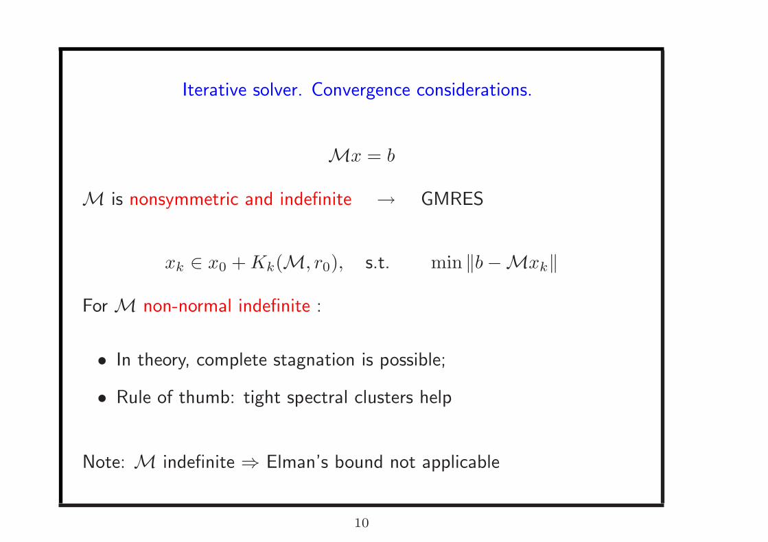
Iterative solver. Convergence considerations.
Mx = b
M is nonsymmetric and indefinite → GMRES
xk ∈ x0 + Kk(M, r0), s.t. min ‖b −Mxk‖
For M non-normal indefinite :
• In theory, complete stagnation is possible;
• Rule of thumb: tight spectral clusters help
Note: M indefinite ⇒ Elman’s bound not applicable
9
Iterative solver. Convergence considerations.
Mx = b
M is nonsymmetric and indefinite → GMRES
xk ∈ x0 + Kk(M, r0), s.t. min ‖b −Mxk‖
For M non-normal indefinite :
• In theory, complete stagnation is possible;
• Rule of thumb: tight spectral clusters help
Note: M indefinite ⇒ Elman’s bound not applicable
10

Rule of thumb: clustering helps
−0.6 −0.4 −0.2 0 0.2 0.4 0.6 0.8 1 1.2 1.4
−3
−2
−1
0
1
2
3
11

GMRES: Nonstagnation condition (Simoncini & Szyld, ’08)
Let H = 1
2(M + M⊤), S = 1
2(M−M⊤). If
H nonsingular and ‖SH−1‖ < 1
Then
‖r2‖ ≤(
1 − θ2min
‖M2‖2
) 1
2
‖r0‖ θmin = λmin( 1
2(M2 + (M2)⊤)) > 0
The same relation holds at every other iteration
12

M symmetric indefinite. Well-exercised spectral properties
M =
A B⊤
B O
0 < λn ≤ · · · ≤ λ1 eigs of A
0 < σm ≤ · · · ≤ σ1 sing. vals of B
µ(M) subset of (Rusten & Winther 1992)
»1
2(λn −
qλ2
n + 4σ21),
1
2(λ1 −
qλ21
+ 4σ2m)
–∪
»λn,
1
2(λ1 +
qλ21
+ 4σ21)
–
xxxx
13
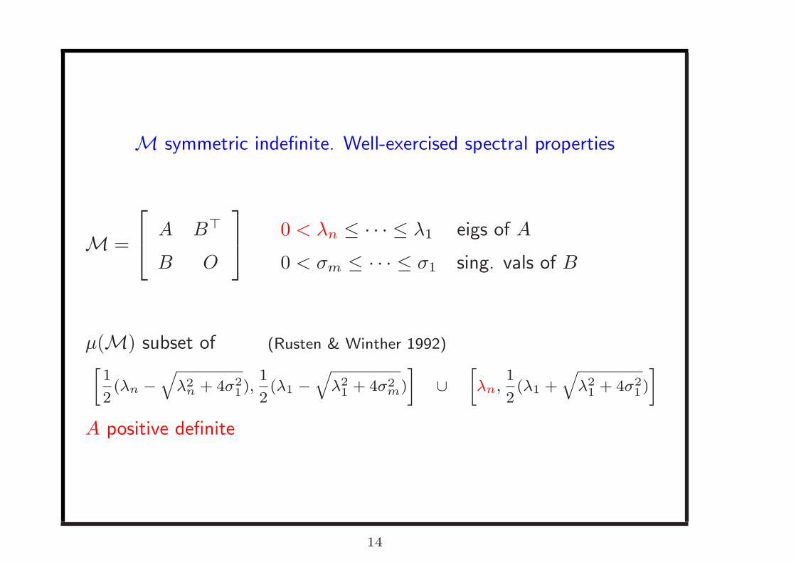
M symmetric indefinite. Well-exercised spectral properties
M =
A B⊤
B O
0 < λn ≤ · · · ≤ λ1 eigs of A
0 < σm ≤ · · · ≤ σ1 sing. vals of B
µ(M) subset of (Rusten & Winther 1992)
»1
2(λn −
qλ2
n + 4σ21),
1
2(λ1 −
qλ21
+ 4σ2m)
–∪
»λn,
1
2(λ1 +
qλ21
+ 4σ21)
–
A positive definite
14

M symmetric indefinite. Well-exercised spectral properties
M =
A B⊤
B O
0 = λn ≤ · · · ≤ λ1 eigs of A
0 < σm ≤ · · · ≤ σ1 sing. vals of B
µ(M) subset of»
1
2(λn −
qλ2
n + 4σ21),
1
2(λ1 −
qλ21
+ 4σ2m)
–∪
»α0,
1
2(λ1 +
qλ21
+ 4σ21)
–
A semidefinite but u⊤Auu⊤u
> α0 > 0, u ∈ Ker(B) Perugia & S., ’00
15

M symmetric indefinite. Well-exercised spectral properties
M =
A B⊤
B O
0 < λn ≤ · · · ≤ λ1 eigs of A
0 < σm ≤ · · · ≤ σ1 sing. vals of B
µ(M) subset of (Rusten & Winther 1992)
»1
2(λn −
qλ2
n + 4σ21),
1
2(λ1 −
qλ21
+ 4σ2m)
–∪
»λn,
1
2(λ1 +
qλ21
+ 4σ21)
–
B full rank
16

M symmetric indefinite. Well-exercised spectral properties
M =
A B⊤
B −C
0 < λn ≤ · · · ≤ λ1 eigs of A
0 = σm ≤ · · · ≤ σ1 sing. vals of B
µ(M) subset of (Silvester & Wathen 1994)
»1
2(−γ1 + λn −
q(γ1 + λn)2 + 4σ2
1) ,
1
2(λ1 −
qλ21
+ 4θ)
–∪
»λn,
1
2(λ1 +
qλ21
+ 4σ21)
–
B rank deficient, but θ = λmin(BB⊤ + C) full rank
γ1 = λmax(C)
17
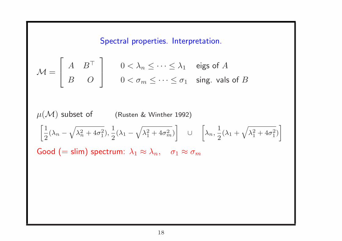
Spectral properties. Interpretation.
M =
A B⊤
B O
0 < λn ≤ · · · ≤ λ1 eigs of A
0 < σm ≤ · · · ≤ σ1 sing. vals of B
µ(M) subset of (Rusten & Winther 1992)
»1
2(λn −
qλ2
n + 4σ21),
1
2(λ1 −
qλ21
+ 4σ2m)
–∪
»λn,
1
2(λ1 +
qλ21
+ 4σ21)
–
Good (= slim) spectrum: λ1 ≈ λn, σ1 ≈ σm
e.g.
M =
I U⊤
U O
, UU⊤ = I
18

Spectral properties. Interpretation.
M =
A B⊤
B O
0 < λn ≤ · · · ≤ λ1 eigs of A
0 < σm ≤ · · · ≤ σ1 sing. vals of B
µ(M) subset of (Rusten & Winther 1992)
»1
2(λn −
qλ2
n + 4σ21),
1
2(λ1 −
qλ21
+ 4σ2m)
–∪
»λn,
1
2(λ1 +
qλ21
+ 4σ21)
–
Good (= slim) spectrum: λ1 ≈ λn, σ1 ≈ σm
e.g.
M =
I U⊤
U O
, UU⊤ = I
19

Block diagonal Preconditioner
⋆ A spd, C = 0:
P0 =
A 0
0 BA−1B⊤
⇒ P−1
2
0MP−
1
2
0=
24 I A−
1
2 B⊤(BA−1B⊤)−1
2
(BA−1B⊤)−1
2 BA−1
2 0
35
MINRES converges in at most 3 iterations. µ(P−1
2
0MP−
1
2
0) = {1, 1/2 ±
√5/2}
A more practical choice:
P =
A 0
0 S
spd. A ≈ A S ≈ BA−1B⊤
eigs in [−a,−b] ∪ [c, d], a, b, c, d > 0
Still an Indefinite Problem, but possibly much easier to solve
20

Block diagonal Preconditioner
⋆ A spd, C = 0:
P0 =
A 0
0 BA−1B⊤
⇒ P−1
2
0MP−
1
2
0=
24 I A−
1
2 B⊤(BA−1B⊤)−1
2
(BA−1B⊤)−1
2 BA−1
2 0
35
MINRES converges in at most 3 iterations. µ(P−1
2
0MP−
1
2
0) = {1, 1/2 ±
√5/2}
A more practical choice:
P =
A 0
0 S
spd. A ≈ A S ≈ BA−1B⊤
eigs in [−a,−b] ∪ [c, d], a, b, c, d > 0
Still an Indefinite Problem, but possibly much easier to solve
21

Indefinite A
M =
A B⊤
B O
λn ≤ · · · ≤ λ1 eigs of A
0 < σm ≤ · · · ≤ σ1 sing. vals of B
A pos.def. on Ker(B)
σ(M) subset of»
1
2(λn −
qλ2
n + 4σ21),
1
2(λ1 −
qλ21
+ 4σ2m)
–∪
»Γ,
1
2(λ1 +
qλ21
+ 4σ21)
–
If m = n, Γ = 1
2(λn +
√λ2
n + 4σ2m)
22
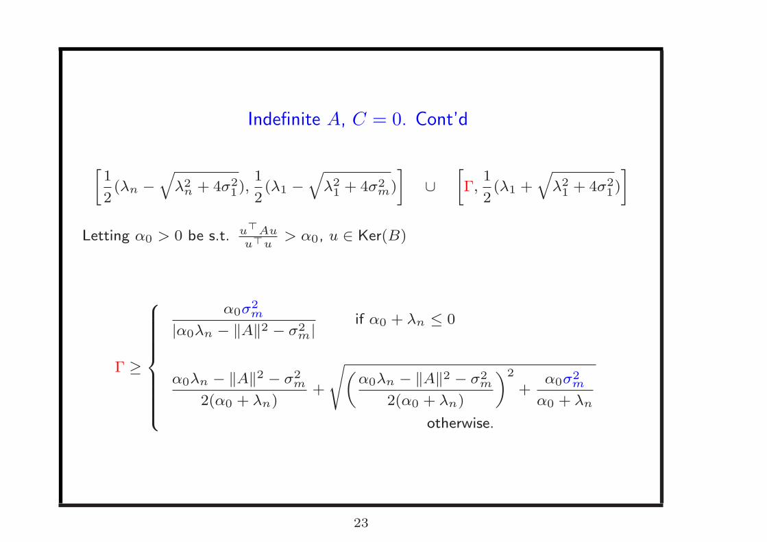
Indefinite A, C = 0. Cont’d
»1
2(λn −
qλ2
n + 4σ21),
1
2(λ1 −
qλ21
+ 4σ2m)
–∪
»Γ,
1
2(λ1 +
qλ21
+ 4σ21)
–
Letting α0 > 0 be s.t. u⊤Au
u⊤u> α0, u ∈ Ker(B)
Γ ≥
8>>>>>>>><>>>>>>>>:
α0σ2m
|α0λn − ‖A‖2 − σ2m| if α0 + λn ≤ 0
α0λn − ‖A‖2 − σ2m
2(α0 + λn)+
s„α0λn − ‖A‖2 − σ2
m
2(α0 + λn)
«2
+α0σ2
m
α0 + λn
otherwise.
23

Sharpness of the bounds
Ex.1. A =
24 1 −3
−3 2
35 , B⊤ =
24 0
0.1
35 µ(M) = {−1.5441, 0.0014257, 4.5427}
Ex.2. A =
24 0.01 3
3 −0.01
35 , B = [0, 3] µ(M) = {−4.2452, 5.0 · 10−3, 4.2402}
Ex.3. A =
2664
1 −4 0
−4 −1 0
0 0 2
3775 , B⊤ =
2664
0 1
1 0
0 0
3775 , µ(M) =
{−4.3528, −0.22974,
0.22974, 2, 4.3528}
case λn λ1 α0 σm, σ1 I− I+
Ex.1 -1.5414 4.5414 1.0 0.1 [-1.5478, -0.0022] [0.0004, 4.5436]
Ex.2 -3.0000 3.0000 0.01 3 [-4.8541, -1.8541] [ 4.9917 ·10−3, 4.8541]
Ex.3 -4.1231 4.1231 2.0 1 [-4.3528, -0.22974] [0.0762, 4.3528]
24

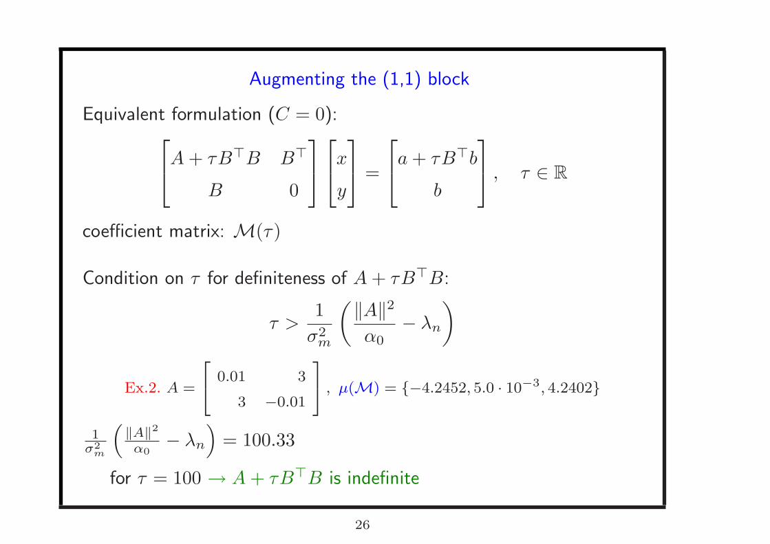
Augmenting the (1,1) block
Equivalent formulation (C = 0):A + τB⊤B B⊤
B 0
x
y
=
a + τB⊤b
b
, τ ∈ R
coefficient matrix: M(τ)
Condition on τ for definiteness of A + τB⊤B:
τ >1
σ2m
(‖A‖2
α0
− λn
)
Ex.2. A =
24 0.01 3
3 −0.01
35 , µ(M) = {−4.2452, 5.0 · 10−3, 4.2402}
1
σ2m
(‖A‖2
α0
− λn
)= 100.33
for τ = 100 → A + τB⊤B is indefinite
25
Augmenting the (1,1) block
Equivalent formulation (C = 0):A + τB⊤B B⊤
B 0
x
y
=
a + τB⊤b
b
, τ ∈ R
coefficient matrix: M(τ)
Condition on τ for definiteness of A + τB⊤B:
τ >1
σ2m
(‖A‖2
α0
− λn
)
Ex.2. A =
24 0.01 3
3 −0.01
35 , µ(M) = {−4.2452, 5.0 · 10−3, 4.2402}
1
σ2m
(‖A‖2
α0
− λn
)= 100.33
for τ = 100 → A + τB⊤B is indefinite
26

Augmenting the (1,1) block
Assume “good” τ is taken.
A + τB⊤B B⊤
B 0
x
y
=
a + τB⊤b
b
, τ ∈ R
Spectral intervals for (1,1) spd may be obtained
27

“Regularized” problemA B⊤
B −C
x
y
=
a + τB⊤b
b
, τ ∈ R
Coefficient matrix: MC
Warning: for A indefinite, conditions on C required:−1 1
1 −1
singular!
Note: Perturbation results yield spectral bounds assuming λCmax < Γ
28

“Regularized” problem
More accurate result:
If λCmax <
α0σ2
m
‖A‖2−λnα0
, then µ(MC) ⊂ I− ∪ I+ with
I− =
»1
2
„λn − λC
max −q
(λn + λCmax)2 + 4σ2
1
«,1
2
„λ1 −
q(λ1)2 + 4σ2
m
«–⊂ R
−
I+ =
»ΓC ,
1
2
„λ1 +
q(λ1)2 + 4σ2
1
«–⊂ R
+,
For m = n, ΓC = 1
2
(λn − λC
max +√
(λn + λCmax)
2 + 4σ2m
)
more complicated (but explicit!) estimate for m < n
29
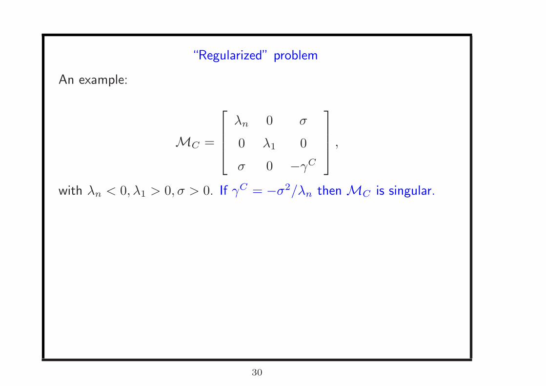
“Regularized” problem
An example:
MC =
λn 0 σ
0 λ1 0
σ 0 −γC
,
with λn < 0, λ1 > 0, σ > 0. If γC = −σ2/λn then MC is singular.
Our estimate requires (for ‖A‖ = α0 = −λn): 0 ≤ γC ≤ 1
2
−σ2
λn
(half the value from singularity!)
———————————–
Related result: Bai, Ng, Wang (tech.rep.2008) qualitatively similar
bound based on B⊤C−1B, A + B⊤C−1B
(no full rank assumption on B)
30

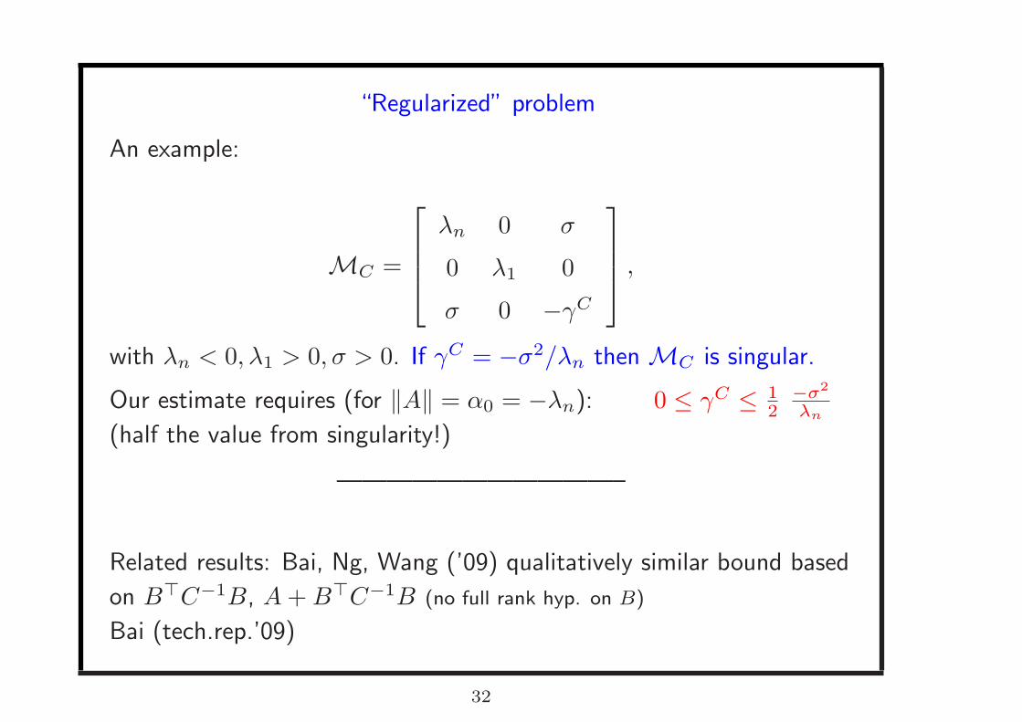
“Regularized” problem
An example:
MC =
λn 0 σ
0 λ1 0
σ 0 −γC
,
with λn < 0, λ1 > 0, σ > 0. If γC = −σ2/λn then MC is singular.
Our estimate requires (for ‖A‖ = α0 = −λn): 0 ≤ γC ≤ 1
2
−σ2
λn
(half the value from singularity!)
———————————–
Related result: Bai, Ng, Wang (tech.rep.2008) qualitatively similar
bound based on B⊤C−1B, A + B⊤C−1B
(no full rank assumption on B)
31
“Regularized” problem
An example:
MC =
λn 0 σ
0 λ1 0
σ 0 −γC
,
with λn < 0, λ1 > 0, σ > 0. If γC = −σ2/λn then MC is singular.
Our estimate requires (for ‖A‖ = α0 = −λn): 0 ≤ γC ≤ 1
2
−σ2
λn
(half the value from singularity!)
———————————–
Related results: Bai, Ng, Wang (’09) qualitatively similar bound based
on B⊤C−1B, A + B⊤C−1B (no full rank hyp. on B)
Bai (tech.rep.’09)
32

Full rank assumption of B
In some optimization problems:
B =
B1
B2
and C =
C1 0
0 0
,
with positive definite C1
Natural assumption: A + B⊤1 C−1
1 B1 definite on the null space of the
full-rank B2. In this case,
MC =
A B⊤
1
B1 −C1
B⊤
2
0
(B2 0
)0
.
Spectral analysis: Use Bai, Ng, Wang result to get spectral intervals
for the “(1,1)” block, and then apply our bounds for MC
33

Application to ideal block diagonal preconditioners
Indefinite preconditioner, C = 0:
1. Let P+ = blkdiag(A, BA−1B⊤). Then
µ(P−1+ M) ⊂
{1,
1
2(1 +
√5),
1
2(1 −
√5)
}⊂ R;
2. Let P− = blkdiag(A,−BA−1B⊤). Then
µ(P−1− M) ⊂
{1,
1
2(1 + i
√3),
1
2(1 − i
√3)
}⊂ C
+.
34
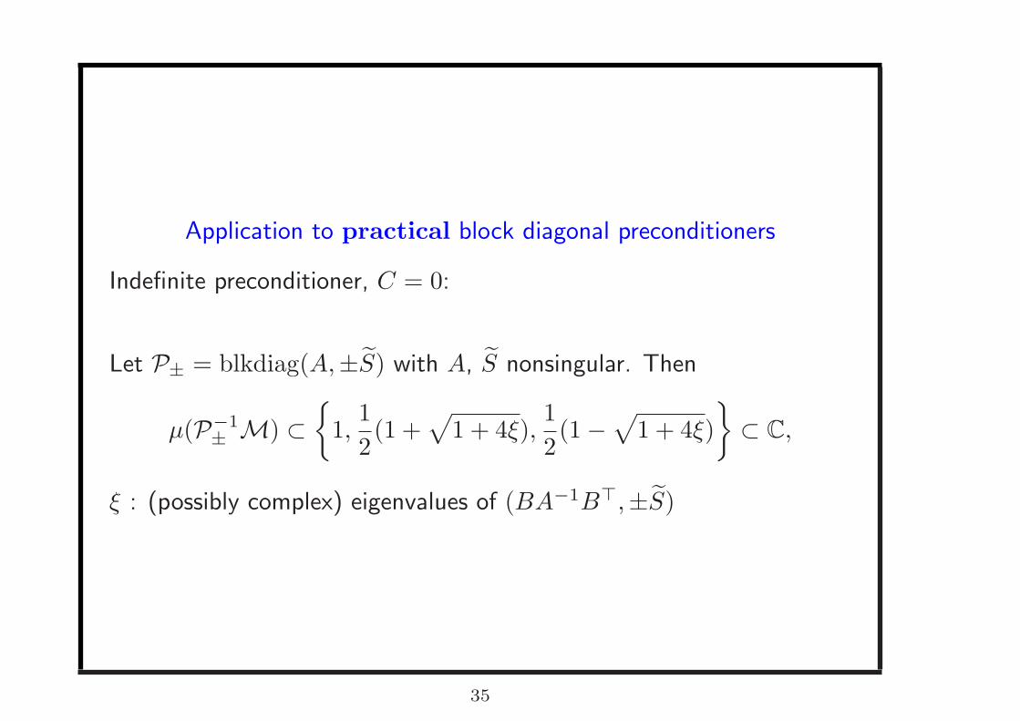
Application to practical block diagonal preconditioners
Indefinite preconditioner, C = 0:
Let P± = blkdiag(A,±S) with A, S nonsingular. Then
µ(P−1± M) ⊂
{1,
1
2(1 +
√1 + 4ξ),
1
2(1 −
√1 + 4ξ)
}⊂ C,
ξ : (possibly complex) eigenvalues of (BA−1B⊤,±S)
35
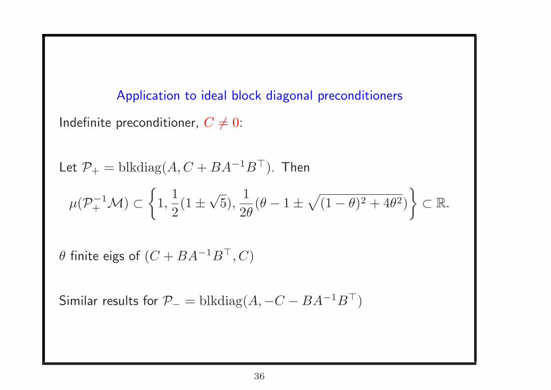
Application to ideal block diagonal preconditioners
Indefinite preconditioner, C 6= 0:
Let P+ = blkdiag(A, C + BA−1B⊤). Then
µ(P−1+ M) ⊂
{1,
1
2(1 ±
√5),
1
2θ(θ − 1 ±
√(1 − θ)2 + 4θ2)
}⊂ R.
θ finite eigs of (C + BA−1B⊤, C)
Similar results for P− = blkdiag(A,−C − BA−1B⊤)
36

Application to ideal block diagonal preconditioners
Definite preconditioner, C = 0:
P(τ) =
PA
PC
,
PA ≈ PA(τ) = A + τB⊤B
PC ≈ PC(τ) = B(A + τB⊤B)−1B⊤
• Definite preconditioner on definite problem:
P(τ)−1M(τ) has eigenvalues
1, 1
2(1 +
√5), 1
2(1 −
√5)
with multiplicity n − m, m and m, respectively.
37
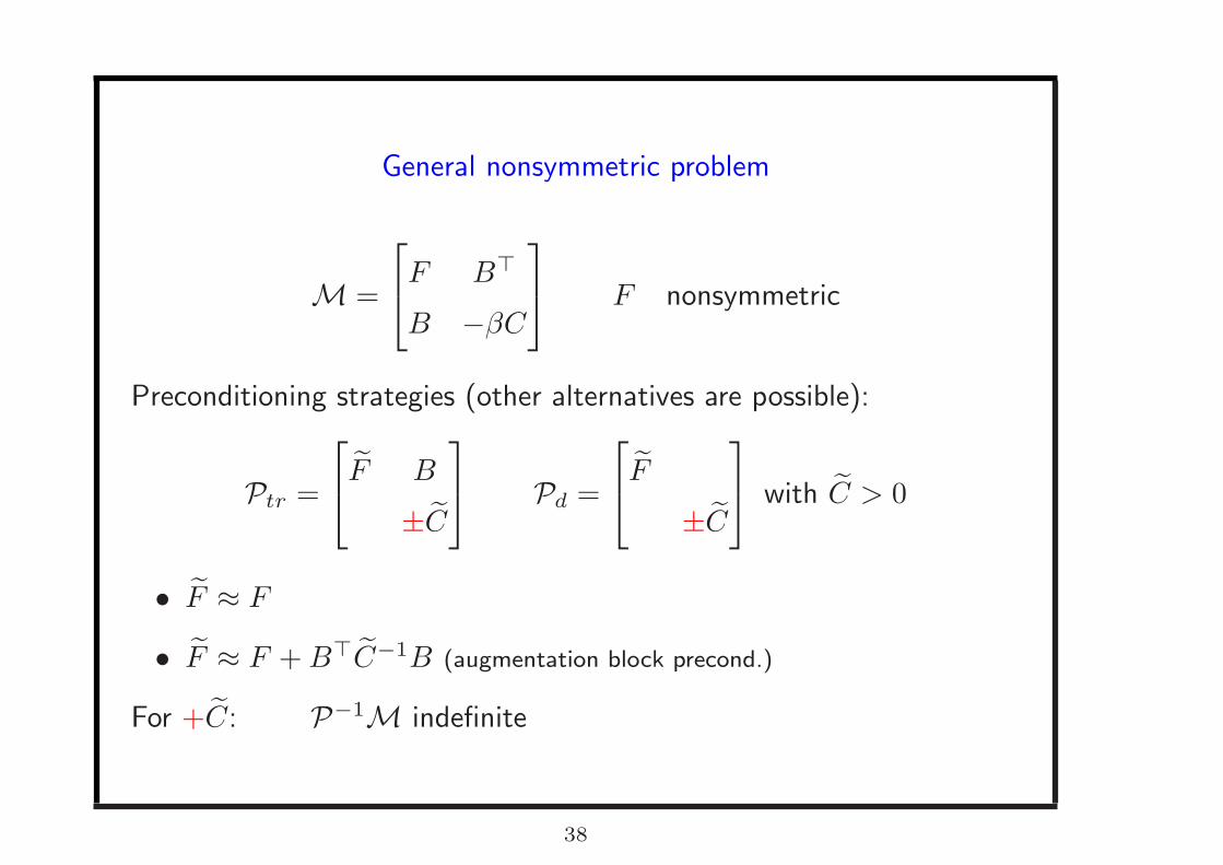
General nonsymmetric problem
M =
F B⊤
B −βC
F nonsymmetric
Preconditioning strategies (other alternatives are possible):
Ptr =
F B
±C
Pd =
F
±C
with C > 0
• F ≈ F
• F ≈ F + B⊤C−1B (augmentation block precond.)
For +C: P−1M indefinite
38

Augmentation block preconditioning
⋆ Appealing for F singular
For +C:
P−1
d M, P−1tr M have clusters in C
− and C+
⇒ Indefinite matrix ⇒ Elman’s bound not applicable
Analysis of clusters:
- Schotzau & Greif ’06 (F sym)
- Cao ’07
39
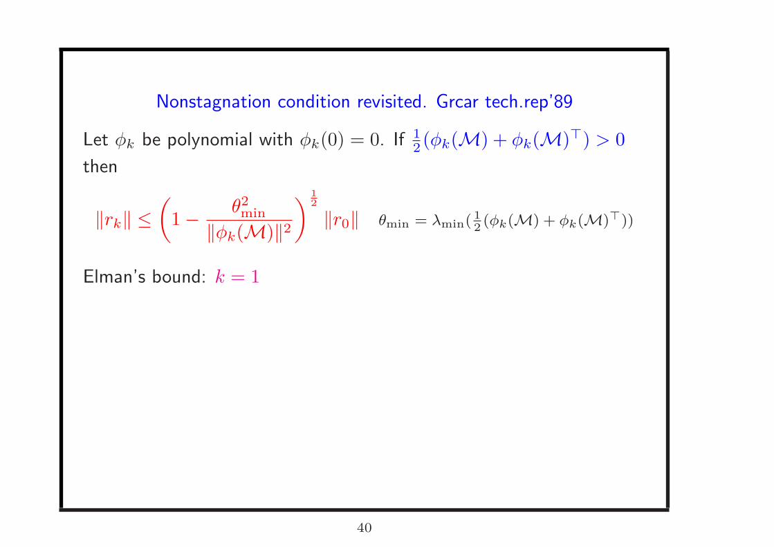
Nonstagnation condition revisited. Grcar tech.rep’89
Let φk be polynomial with φk(0) = 0. If 1
2(φk(M) + φk(M)⊤) > 0
then
‖rk‖ ≤(
1 − θ2min
‖φk(M)‖2
) 1
2
‖r0‖ θmin = λmin( 1
2(φk(M) + φk(M)⊤))
Elman’s bound: k = 1
The simplest case: k = 2
If φ2(H) > 0, then φ2(M) > 0 iff ‖Sφ2(H)−1/2‖ < 1
⇒ In Simoncini & Szyld ’08: φ2(λ) = λ2
⇒ Here: φ2(λ) = λ(λ − α), α = max{0, λ+(H) + λ−(H)}(λ+(H), λ−(H): closest pos/neg eigs to zero)
40
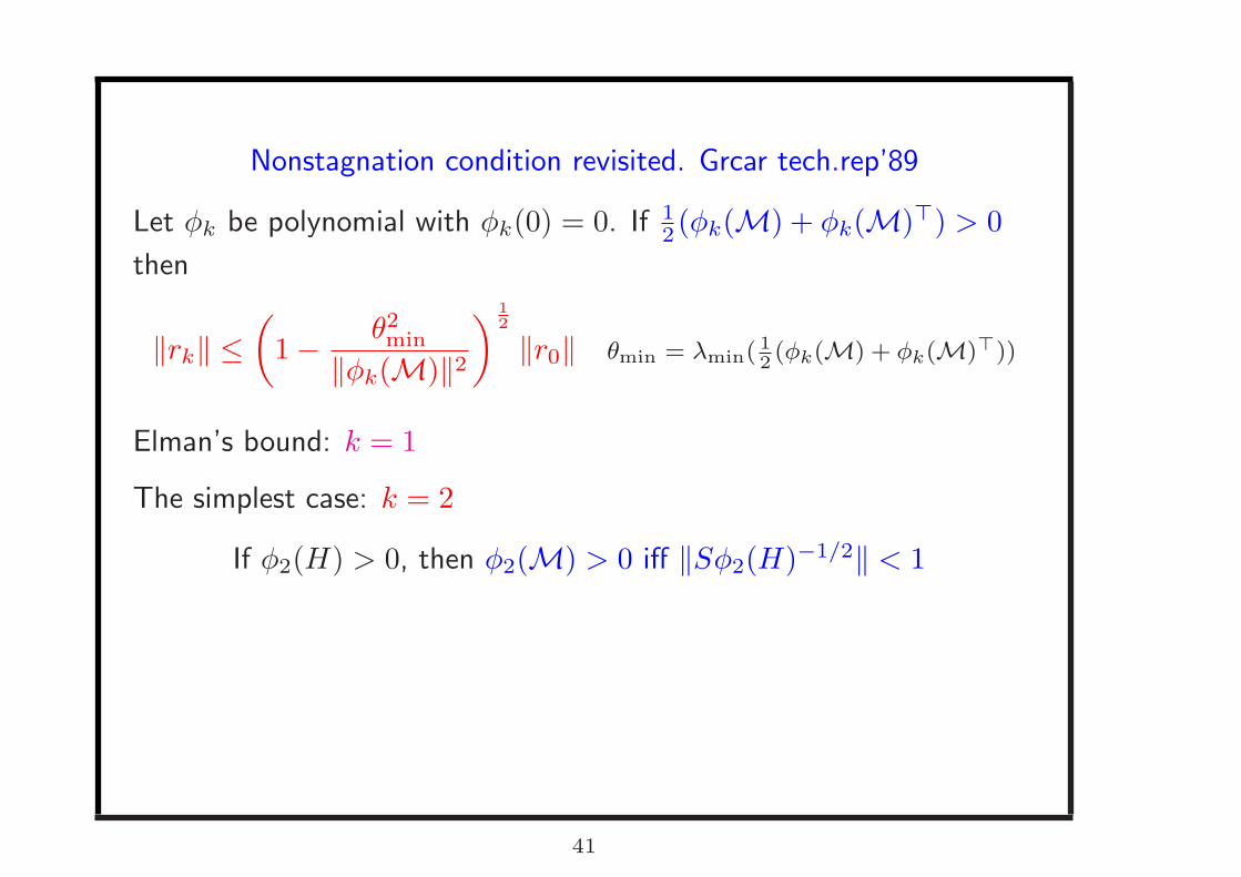
Nonstagnation condition revisited. Grcar tech.rep’89
Let φk be polynomial with φk(0) = 0. If 1
2(φk(M) + φk(M)⊤) > 0
then
‖rk‖ ≤(
1 − θ2min
‖φk(M)‖2
) 1
2
‖r0‖ θmin = λmin( 1
2(φk(M) + φk(M)⊤))
Elman’s bound: k = 1
The simplest case: k = 2
If φ2(H) > 0, then φ2(M) > 0 iff ‖Sφ2(H)−1/2‖ < 1
⇒ In Simoncini & Szyld ’08: φ2(λ) = λ2
⇒ Here: φ2(λ) = λ(λ − α), α = max{0, λ+(H) + λ−(H)}(λ+(H), λ−(H): closest pos/neg eigs to zero)
41
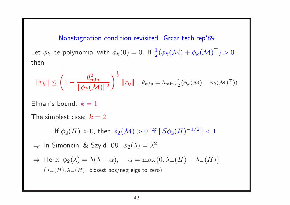
Nonstagnation condition revisited. Grcar tech.rep’89
Let φk be polynomial with φk(0) = 0. If 1
2(φk(M) + φk(M)⊤) > 0
then
‖rk‖ ≤(
1 − θ2min
‖φk(M)‖2
) 1
2
‖r0‖ θmin = λmin( 1
2(φk(M) + φk(M)⊤))
Elman’s bound: k = 1
The simplest case: k = 2
If φ2(H) > 0, then φ2(M) > 0 iff ‖Sφ2(H)−1/2‖ < 1
⇒ In Simoncini & Szyld ’08: φ2(λ) = λ2
⇒ Here: φ2(λ) = λ(λ − α), α = max{0, λ+(H) + λ−(H)}(λ+(H), λ−(H): closest pos/neg eigs to zero)
42
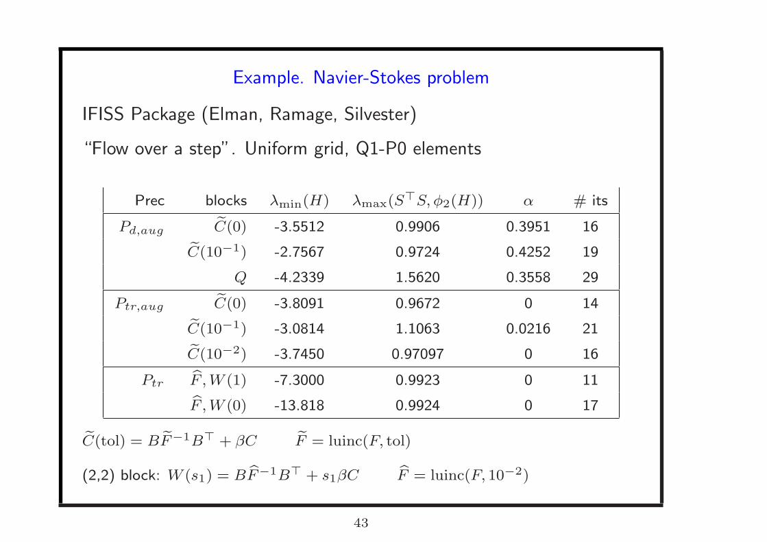
Example. Navier-Stokes problem
IFISS Package (Elman, Ramage, Silvester)
“Flow over a step”. Uniform grid, Q1-P0 elements
Prec blocks λmin(H) λmax(S⊤S, φ2(H)) α # its
Pd,augeC(0) -3.5512 0.9906 0.3951 16
eC(10−1) -2.7567 0.9724 0.4252 19
Q -4.2339 1.5620 0.3558 29
Ptr,augeC(0) -3.8091 0.9672 0 14
eC(10−1) -3.0814 1.1063 0.0216 21
eC(10−2) -3.7450 0.97097 0 16
PtrbF , W (1) -7.3000 0.9923 0 11
bF , W (0) -13.818 0.9924 0 17
eC(tol) = B eF−1B⊤ + βC eF = luinc(F, tol)
(2,2) block: W (s1) = B bF−1B⊤ + s1βC bF = luinc(F, 10−2)
43
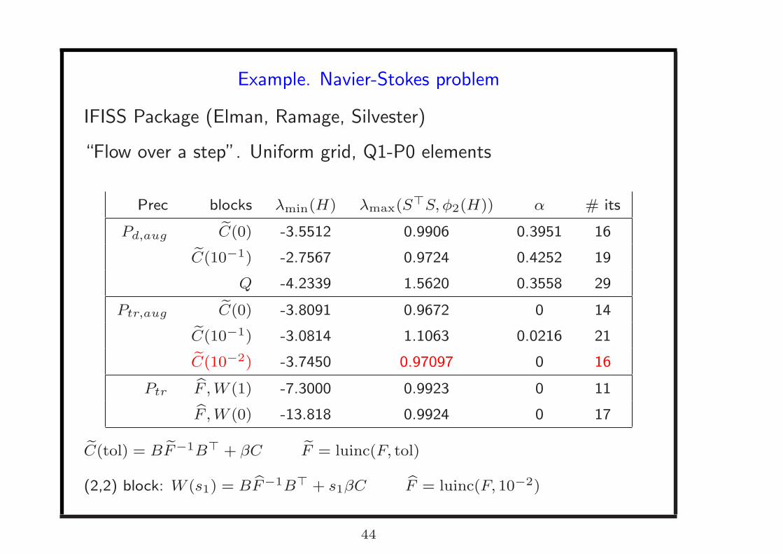
Example. Navier-Stokes problem
IFISS Package (Elman, Ramage, Silvester)
“Flow over a step”. Uniform grid, Q1-P0 elements
Prec blocks λmin(H) λmax(S⊤S, φ2(H)) α # its
Pd,augeC(0) -3.5512 0.9906 0.3951 16
eC(10−1) -2.7567 0.9724 0.4252 19
Q -4.2339 1.5620 0.3558 29
Ptr,augeC(0) -3.8091 0.9672 0 14
eC(10−1) -3.0814 1.1063 0.0216 21
eC(10−2) -3.7450 0.97097 0 16
PtrbF , W (1) -7.3000 0.9923 0 11
bF , W (0) -13.818 0.9924 0 17
eC(tol) = B eF−1B⊤ + βC eF = luinc(F, tol)
(2,2) block: W (s1) = B bF−1B⊤ + s1βC bF = luinc(F, 10−2)
44
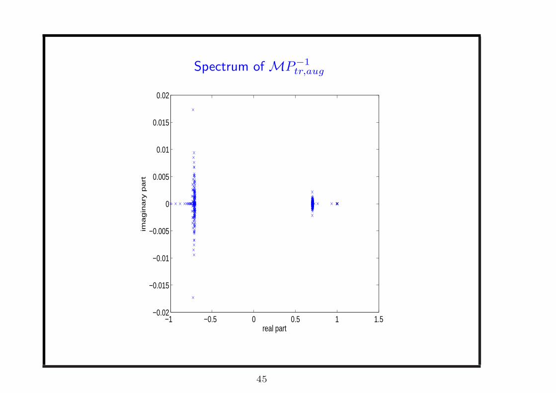
Spectrum of MP−1tr,aug
−1 −0.5 0 0.5 1 1.5−0.02
−0.015
−0.01
−0.005
0
0.005
0.01
0.015
0.02
real part
ima
gin
ary
pa
rt
45

GMRES Convergence history
0 2 4 6 8 10 12 14 1610
−10
10−8
10−6
10−4
10−2
100
number of iterations
no
rm o
f re
sid
ua
l
46
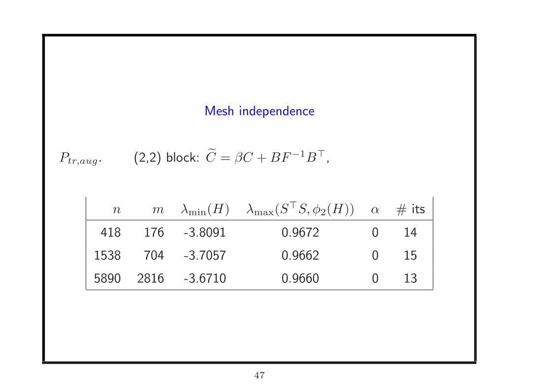
Mesh independence
Ptr,aug. (2,2) block: C = βC + BF−1B⊤,
n m λmin(H) λmax(S⊤S, φ2(H)) α # its
418 176 -3.8091 0.9672 0 14
1538 704 -3.7057 0.9662 0 15
5890 2816 -3.6710 0.9660 0 13
47
Final considerations and outlook
Symmetric case:
• Sharp bounds obtained for symmetric indefinite (1,1) block
• Future work: exploit this knowledge to devise and analyze effective
preconditioners
Nonsymmetric case:
• First attempt to provide convergence information on indefinite
problem
• Future work: devise more complete convergence analysis
48
Final considerations and outlook
Symmetric case:
• Sharp bounds obtained for symmetric indefinite (1,1) block
• Future work: exploit this knowledge to devise and analyze effective
preconditioners
Nonsymmetric case:
• First attempt to provide convergence information on indefinite
problem
• Future work: devise more complete convergence analysis
49
References
1. V. S. and Daniel B. Szyld , New conditions for non-stagnation of
minimal residual methods. Numerische Mathematik, v. 109, n.3
(2008), pp. 477-487.
2. Nick Gould and V. S., Spectral Analysis of saddle point matrices
with indefinite leading blocks. August 2008, To appear in SIAM J.
Matrix Analysis Appl.
3. V.S., On the non-stagnation condition for GMRES and application
to saddle point matrices, In preparation.
50