vacuum membrane
TRANSCRIPT

Desalination 274 (2011) 120–129
Contents lists available at ScienceDirect
Desalination
j ourna l homepage: www.e lsev ie r.com/ locate /desa l
Computational fluid dynamics numerical simulation of vacuum membranedistillation for aqueous NaCl solution
Na Tang ⁎, Huanju Zhang, Wei WangCollege of Marine Science and Engineering, Tianjin University of Science and Technology, Tianjin 300457, PR ChinaTianjin Key Laboratory of Marine Resources and Chemistry, Tianjin 300457, PR China
⁎ Corresponding author at: College of Marine ScieUniversity of Science and Technology, Tianjin 300457, PRfax: +86 22 60600358.
E-mail address: [email protected] (N. Tang).
0011-9164/$ – see front matter © 2011 Elsevier B.V. Adoi:10.1016/j.desal.2011.01.078
a b s t r a c t
a r t i c l e i n f oArticle history:Received 26 November 2010Received in revised form 28 January 2011Accepted 31 January 2011Available online 16 March 2011
Keywords:Aqueous NaCl solutionFLUENTVMDNumerical simulation
Vacuum membrane distillation (VMD) was considered as the multiphase flow (liquid and gas phase) processinside the porous media, and the membrane module was simplified to the two-dimensional structure with asingle membrane silk. The simulation has studied the mass transformation and heat transformation of VMDprocess in the porous media, in which aqueous NaCl solution was seemed as an incompressible and steadyfluid. In the processes of mass transfer, heat transfer and phase transition, all particles were supposed in localthermodynamic balance. By means of FLUENT, one of the softwares about computational fluid dynamics(CFD), the numerical simulation of the two-dimensional model of VMD for aqueous NaCl solution wasestablished under the steady state. The paper also calculated and analyzed the volume rate of vapor withdifferent feed temperatures.
nce and Engineering, TianjinChina. Tel.: +86 22 60601158;
ll rights reserved.
© 2011 Elsevier B.V. All rights reserved.
1. Introduction
Membrane distillation (MD) is an evaporation process of feedvolatile components through a porous hydrophobic membrane [1],and the driving force is the vapor pressure difference on both sidesof the membrane [2]. According to the different condensing andremoving methods of volatile component vapor on cold side, MD canbe divided into the following four kinds: direct contact membranedistillation (DCMD), air gap membrane distillation (AGMD), vacuummembrane distillation (VMD) and sweeping gas membrane distilla-tion (SGMD) [3].
As a new membrane separation technology, VMD has been de-veloped in recent years. It is a process in which the hot solution flowsthrough one side of the membrane [4] and vacuum is applied in thepermeate side. The vapor pressure difference is formed on both sidesof the membrane for mass transfer, meanwhile the evaporable sub-stance is separated from the permeate side and be condensed intoliquid, therefore concentration and separation of the solution areimplemented effectively. Compared to other MD processes, one ofthe advantages of VMD is that the heat conduction loss through themembrane is negligible. Because the produced vapor was vacuumizedinto a condenser, the pressure on the cold side of the membrane ismuch lower, and a higher flux can be obtained in the VMD process.
VMD is a process in which mass transfer and heat transfer occursimultaneously. The mass transfer for aqueous NaCl solution in VMDrefers to the process of water molecules transferring from the hotside to the cold side, which can be divided into 4 steps: (1) watermolecules transfer from the hot solution bulk to the hot side of themembrane surface; (2) water of the NaCl aqueous solution vaporizeon the hot side of the membrane; (3) water vapor diffuses fromthe hot side of the membrane surface through pores to the cold side;(4) water vapor is condensed in the condensing system, accordingly.Heat transfer process is divided into five steps: (1) heat transfer fromthe hot solution bulk through the boundary layer to the hot side ofthe membrane surface; (2) part of the heat on the hot side of themembrane provides the vaporization heat for vaporization; (3) heattransfers from the hot side of the membrane surface through pores tothe cold side; (4) water vapor on the cold side condenses and releasesthe vaporization heat; (5) heat transfers from the cold side of themembrane surface to the condensing system.
The main process parameters that influence the VMD process arethe structure parameters of the membrane (including average poresize, porosity, curvature, thickness, etc.) and the process operatingparameters (temperature, pressure, flow rate, concentration, vacuumdegree, etc.).
At present, methods with which the separation performance ofhollow fiber membrane module can be described quantitatively in-clude mathematical model method and the empirical correlationmethod. However, themathematical model methodmostly bases on asimplified geometry and flowing state assumptions of the separationperformance of the membrane module, which does not reflect theeffects of the important factors such as turbulence etc. Another idea is

121N. Tang et al. / Desalination 274 (2011) 120–129
to create a specific type of empirical correlation for membranemodules. While, in terms of geometric features of the membrane,the application scope of the correlations that exist in the literaturesis rather small, causing significant limitations on its application.Computational fluid dynamics method can solve the above-men-tioned problems. Computational fluid dynamics (CFD) is an effectiveapproach for solving the related physical phenomena such as the flowand heat conduction of fluid numerically by means of computationalnumerical calculation and image display [5]. FLUENT is a typicalcommercial software package of CFD, which is powerful and can beused widely.
In the related studies of membrane process, the reference aboutapplying CFD to the membrane process is rarely found. Randomsequential addition (RSA) algorithm was utilized to develop a three-dimensional geometric model for gas–liquid cocontactor of hollowfiber membrane modules by Yiyang etc. The result shows that higherReynolds number yields better shell-side mass transfer. Under lowpacking density, convection is significant in shell-side flow, which ispreferable for the reduction of dead zone area and the higher uti-lization of contacting area. On the other hand, increasing packingdensity will result in a higher ratio area for the contactor, but at thesame time may reduce the significance of convection in mass transfer,and renderingwaste of themembrane surface [6]. XiaojuanQi adoptedrotational tangential inpouring to increase the turbulence intensityand the flow velocity near the membrane, leading to the decreasing ofthe temperature and concentration boundary thicknesses. They alsosimulated the temperature and flow field in a hot cavity circulationsystem of AGMDwithwater as thematerial by CFD. The result verifiedthat temperature gradient near the membrane would reduce greatlywith rotational tangential inpouring, and different tangential inpour-ing angle and spout shape had great influence on the temperaturegradient [7].
In this paper, CFD was used as a tool, and the appropriate sim-ulation models were selected to study the fluid dynamics of VMD.
2. The choice of mathematical models and the control equations
VMDwas considered as themultiphase flow (liquid and gas phase)process inside the porousmedia in the simulation. So multiphase flowmodel was chosen, and porous media condition was set.
2.1. The choice of multiphase flow model
There are three multiphase flow models in CFD simulation: VOFmodel (Volume of Fluid Model), Mixture Model and Eulerian Model.Since the simulation involved the uniform flow of the gas, mixedmodel was adopted [8]. Mixed model is a simplified multiphase flowmodel, which is the good replacement of the Eulerian model inmany situations [9]. A perfect multiphase flow model is infeasiblein the following conditions: there is a wide range of particle dis-tribution; the rules of the interface are unknown; the reliability ofwhich is in doubt. While once the number of variables is less thanthe perfect multiphase flow model, the simple model such as themixed model can obtain as good results as that of the multiphaseflow model.
The mixture model solves the continuity equation for the mix-ture, the momentum equation for the mixture, the energy equationfor the mixture, and the volume fraction equation for the secondaryphases, as well as algebraic expressions for the relative velocities(if the phases are moving at different velocities). And the processof using the mixture model to solve the problem is as follows:(1) chose “mixture” on the “multiphasemodel” plate; (2) set “phase-1” to liquid and “phase-2” to vapor; (3) check and modify thematerial of fluid.
2.2. Conservation equations
According to the mixture model, the continuity equation is
∂∂t ρmð Þ + ∇⋅ ρmυm
� �= 0 ð1Þ
Where υm is the mass-averaged velocity:
υm =∑n
k=1αkρkυk
ρmð2Þ
where, ρm is the mixture density:
ρm = ∑n
k=1αkρk ð3Þ
where, αk is the volume fraction of phaseκ.The momentum equation for the mixture can be obtained by
summing the individual momentum equations for all phases. It can beexpressed as Eq. (4):
∂∂t ρmυm
� �+ ∇⋅ ρmυmυm
� �= −∇p + ∇⋅ μm ∇υm + ∇υT
m
� �h i
+ ρmg +→F + ∇⋅ ∑
n
k=1αkρk
→υdr;k→υdr;k
� �ð4Þ
where, n is the number of phases,→F is a body force, and μm is the
viscosity of the mixture.
μm = ∑n
k=1αkμk ð5Þ
where, →υdr;k is the drift velocity for secondary phase k:
→υdr;k = υk−υm: ð6Þ
The energy equation for the mixture takes the following Eq. (7).
∂∂t ∑
n
k=1αkρkEkð Þ + ∇ ∑
n
k=1αkυk ρkEk + pð Þ� �
= ∇⋅ keff∇T� �
+ SE ð7Þ
where keff is the effective conductivity (∑αk(kk+kt)), where kt is theturbulent thermal conductivity, defined according to the turbulencemodel being used. The first term on the right-hand side of Eq. (7)represents the energy transfer due to conduction, where SEincludesany other volumetric heat sources.
In Eq. (7):
Ek = hk−pρk
+υ2k
2: ð8Þ
2.3. The choice of the viscous model
In CFD simulation, the main viscous models are: inviscid model,laminar model, Spalart–Allmaras model (one equation), k-epsilonmodel (two equations) and Reynolds Stress model (two equations).Here, k-epsilonmodel refers to standard k-εmodel firstly. While, afterthe researchers followed and amended the standard κ-ε model, theRNG k-ε model and the realizable k-ε model have been developed.
In the study, standard k-ε model was adopted to simulate theturbulent flow field in the membrane module. The numerical solutionof k and ε can be reached by solving the turbulence kinetic energy kand its rate of dissipation ε [10], with which the turbulent viscositywould be calculated. Finally the number of Reynolds stress [11] can bederived by Boussinesq hypothesis.

Table 1The main dimension parameters of the membrane and the membrane silk.
Membrane Length Outer diameter Inner diameter Export/import diameter Export/import length Vacuum outlet diameter300 mm Φ40 mm Φ30 mm Φ5 mm 20 mm Φ5 mm
Membrane silk Length Outer diameter Inner diameter Porosity290 mm Φ2 mm Φ1 mm 85%
122 N. Tang et al. / Desalination 274 (2011) 120–129
2.4. Porous media hypothesis
The porous media model employs empirical formulas to define theflow resistance. In essence, porous media is modeled by the additionof momentum source term consumption to the standard momentumequations. Consequently, for the porous media model, the followingmodeling assumptions and limitations should be satisfied:
1) To ensure continuity of the velocity vectors across the porousmedium interface, default FLUENT uses a superficial velocity insidethe porous medium under the default condition.
2) The influence of the porous media on the turbulence field isnothing but approximation.
3) Adding amomentum source term to themomentum equations cansimulate the function of porous media [12–17]. The source term iscomposed of two parts: a viscous loss term—the first term on theright-hand side of equation, and an inertial loss term—the secondterm on the right-hand side of Eq. (9).
Si = − ∑3
j=1Dijμυj + ∑
3
j=1Cij
12ρ υj jυj
!ð9Þ
where Si is the source term for the ith (x, y, or z) momentumequation, D and C are given matrices. A negative source term iscalled “sink”. The momentum sink contributes to the pressuregradient in the porous unit, and it makes a pressure drop which isproportional to the velocity (or velocity squared) of the fluid.
In laminar flows through porous media, the pressure drop istypically proportional to the velocity, and the constant C2 can be set tozero. Ignoring the convective acceleration and diffusion term, theporous media model could be simplified to Darcy's Law [18,19], seenin Eq. (10).
∇p = − μα→υ ð10Þ
3. Geometry model and mesh generation
Polyvinylidene fluoride (PVDF) hollow fiber membrane modulewas used in the simulation. The membrane was purchased fromTianjin Motimo Membrane Technology Co. Ltd. China, and the poresize of the membrane is 0.2 μm, with a porosity of 85%, a membranearea of 0.03768 m2, and a cross section of 7.065×10⁻⁴ m2. The liquid
Fig. 1. Geometric model of the memb
feed was NaCl aqueous solution with a certain concentration of0.5 mol/L. NaCl aqueous solution with high temperature flew into themembrane from the inlet, because the inner section was defined tothe wall except the entry of the membrane silk, so the NaCl aqueoussolution can only flow into the silk, where the water molecule of NaClaqueous solution evaporated and the vapor evaporated from themembrane surface, permeating through the membrane porous intothe cold side of the membrane (membrane shell). The driving force ofthe whole process was vapor pressure difference. The producedvolatile molecules were removed from two vacuum ports at the backof the membrane and were condensed into cold liquid directly orindirectly. The main dimensions of the membrane and the membranesilk were listed in Table 1. Fig. 1 showed the geometric model of themembrane module used for simulation.
Mesh was generated by the commercial grid-generation toolGAMBIT (FLUENT Inc.), and the structured quadrilateral grid wasused. While the automatic mesh partition of membrane silk was bodyfitted anisotropic mesh: the distance from the first mesh point tothe boundary was 0.05, and it was called first row; the growth factorwas 1.01; the creating form was 1:1. The more detailed mesheswere generated for the import and export of the membrane and themembrane silk, vacuum ports. The whole mesh of the model wasshown in Fig. 2.
4. Boundary and initial conditions
4.1. Feed inlet
The inlet region of membrane model was simplified into a rect-angular region, which was set to velocity-inlet. The inlet pressure was1 atmospheric pressure, the velocity was 0.2 m/s, and the gravita-tional acceleration was 9.81 m/s2.
4.2. Outlet
Set to pressure-outlet. For outflow boundary condition, the ve-locity gradient of fluid was assumed to be zero, and the outlet tem-perature was 5 °C lower than the inlet temperature, which is derivedfrom the former experiment [20].
4.3. Vacuum exports
Set to pressure-outlet, the pressure was −0.098 MPa, the tem-perature was 30 °C, and the backflow of vapor was 0.
rane module used for simulation.
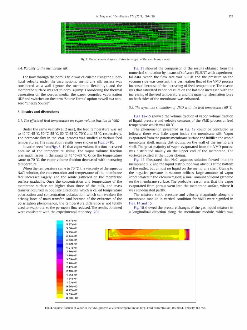
Fig. 2. The schematic diagram of structured grid of the membrane model.
123N. Tang et al. / Desalination 274 (2011) 120–129
4.4. Porosity of the membrane silk
The flow through the porous field was calculated using the super-ficial velocity under the assumptions: membrane silk surface wasconsidered as a wall (ignore the membrane flexibility), and themembrane surface was set to porous-jump. Considering the thermalgeneration on the porous media, the paper compiled vaporizationUDF and switched on the term “Source Terms” option as well as a non-zero “Energy Source”.
5. Results and discussions
5.1. The effects of feed temperature on vapor volume fraction in VMD
Under the same velocity (0.2 m/s), the feed temperature was setto 40 °C, 45 °C, 50 °C, 55 °C, 60 °C, 65 °C, 70°C and 75 °C, respectively.The permeate flux in the VMD process was studied at various feedtemperatures. The simulation results were shown in Figs. 3–10.
It can be seen from Figs. 3–10 that vapor volume fraction increasedbecause of the temperature rising. The vapor volume fractionwas much larger in the range of 45 °C–65 °C. Once the temperaturecame to 70 °C, the vapor volume fraction decreased with increasingtemperature.
When the temperature came to 70 °C, the viscosity of the aqueousNaCl solution, the concentration and temperature of the membraneface increased largely, and the solute gathered on the membranesurface gradually. Once the concentration and temperature of themembrane surface are higher than those of the bulk, and masstransfer occurred in opposite directions, which is called temperaturepolarization and concentration polarization, which can weaken thedriving force of mass transfer. And because of the existence of thepolarization phenomenon, the temperature difference is not totallyused to evaporate, so the permeate flux reduced. The results obtainedwere consistent with the experimental tendency [20].
Fig. 3. Volume fraction of vapor in the VMD process at a feed tempe
Fig. 11 showed the comparison of the results obtained from thenumerical simulation by means of software FLUENT with experimen-tal data. When the flow rate was 50 L/h and the pressure on thevacuum side was constant, the permeation flux of the VMD processincreased because of the increasing of feed temperature. The reasonwas that saturated vapor pressure on the hot side increased with theincreasing of the feed temperature, and themass transformation forceon both sides of the membrane was enhanced.
5.2. The dynamics simulation of VMD with the feed temperature 60 °C
Figs. 12–15 showed the volume fraction of vapor, volume fractionof liquid, pressure and velocity contours of the VMD process at feedtemperature which was 60 °C.
The phenomenon presented in Fig. 12 could be concluded asfollows: there was little vapor inside the membrane silk. Vaporevaporated from the porousmembrane surface and fulfilled thewholemembrane shell, mainly distributing on the wall of the membraneshell. The great majority of vapor evaporated from the VMD processwas distributed mainly on the upper end of the membrane. Thevortexes existed at the upper closing.
Fig. 13 illustrated that NaCl aqueous solution flowed into themembrane silk, and the liquid distribution was obvious at the bottomof the outlet, but almost no liquid on the membrane shell. Owing tothe negative pressure in vacuum orifices, large amounts of vaporconcentrated in the vacuum region; a small amount of liquid gatheredon the membrane surface. The probable reason was that the vaporevaporated from porous went into the membrane surface, where itwas condensated partly.
The mixture static pressure and velocity magnitude along themembrane module in vertical condition for VMD were signified inFigs. 14 and 15.
Fig. 16 showed the pressure changes of the gas–liquid mixture ina longitudinal direction along the membrane module, which was
rature of 40 °C. Feed concentration: 0.5 mol/L; velocity: 0.2 m/s.

Fig. 5. Volume fraction of vapor in the VMD process at a feed temperature of 50 °C. Feed concentration: 0.5 mol/L; velocity: 0.2 m/s.
Fig. 4. Volume fraction of vapor in the VMD process at a feed temperature of 45 °C. Feed concentration: 0.5 mol/L; velocity: 0.2 m/s.
Fig. 6. Volume fraction of vapor in the VMD process at a feed temperature of 55 °C. Feed concentration: 0.5 mol/L; velocity: 0.2 m/s.
124 N. Tang et al. / Desalination 274 (2011) 120–129
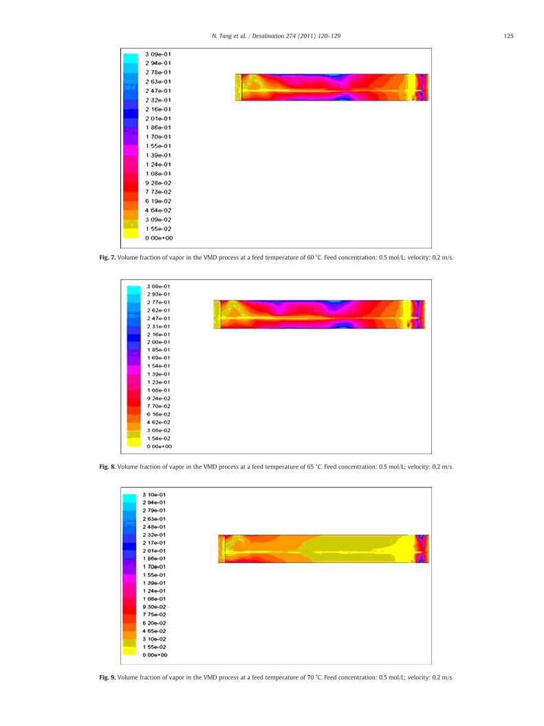
Fig. 7. Volume fraction of vapor in the VMD process at a feed temperature of 60 °C. Feed concentration: 0.5 mol/L; velocity: 0.2 m/s.
Fig. 8. Volume fraction of vapor in the VMD process at a feed temperature of 65 °C. Feed concentration: 0.5 mol/L; velocity: 0.2 m/s.
Fig. 9. Volume fraction of vapor in the VMD process at a feed temperature of 70 °C. Feed concentration: 0.5 mol/L; velocity: 0.2 m/s.
125N. Tang et al. / Desalination 274 (2011) 120–129
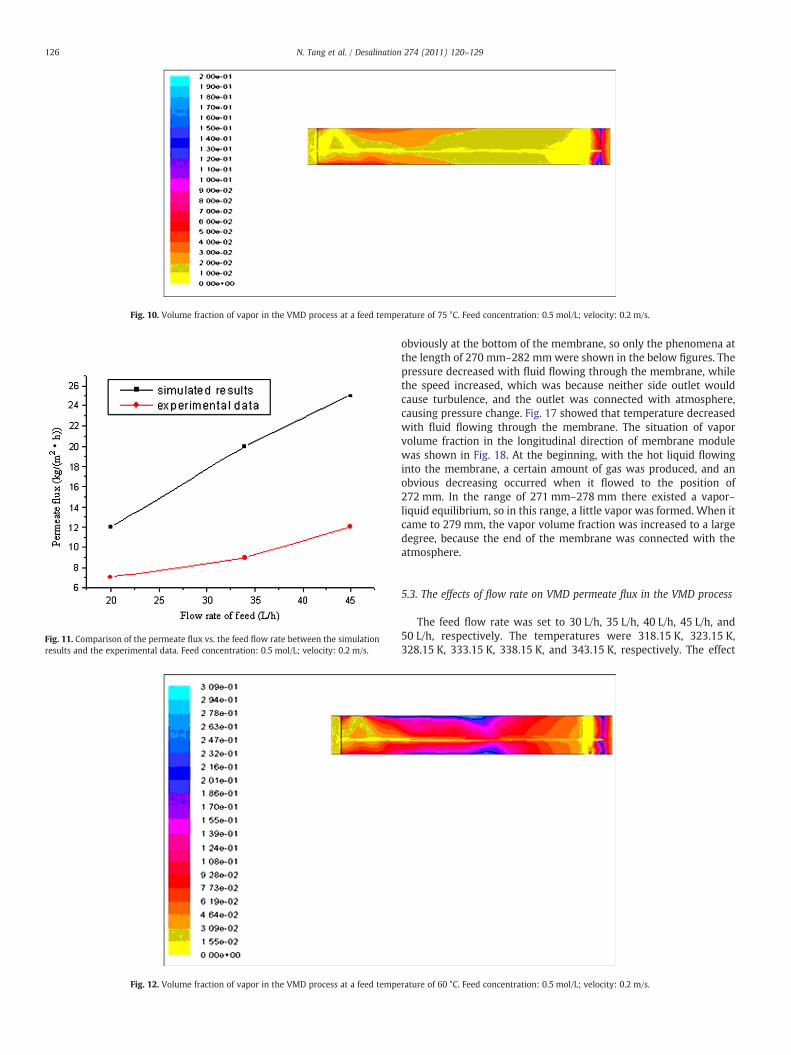
Fig. 10. Volume fraction of vapor in the VMD process at a feed temperature of 75 °C. Feed concentration: 0.5 mol/L; velocity: 0.2 m/s.
Fig. 11. Comparison of the permeate flux vs. the feed flow rate between the simulationresults and the experimental data. Feed concentration: 0.5 mol/L; velocity: 0.2 m/s.
Fig. 12. Volume fraction of vapor in the VMD process at a feed tempe
126 N. Tang et al. / Desalination 274 (2011) 120–129
obviously at the bottom of the membrane, so only the phenomena atthe length of 270 mm–282 mm were shown in the below figures. Thepressure decreased with fluid flowing through the membrane, whilethe speed increased, which was because neither side outlet wouldcause turbulence, and the outlet was connected with atmosphere,causing pressure change. Fig. 17 showed that temperature decreasedwith fluid flowing through the membrane. The situation of vaporvolume fraction in the longitudinal direction of membrane modulewas shown in Fig. 18. At the beginning, with the hot liquid flowinginto the membrane, a certain amount of gas was produced, and anobvious decreasing occurred when it flowed to the position of272 mm. In the range of 271 mm–278 mm there existed a vapor–liquid equilibrium, so in this range, a little vapor was formed. When itcame to 279 mm, the vapor volume fraction was increased to a largedegree, because the end of the membrane was connected with theatmosphere.
5.3. The effects of flow rate on VMD permeate flux in the VMD process
The feed flow rate was set to 30 L/h, 35 L/h, 40 L/h, 45 L/h, and50 L/h, respectively. The temperatures were 318.15 K, 323.15 K,328.15 K, 333.15 K, 338.15 K, and 343.15 K, respectively. The effect
rature of 60 °C. Feed concentration: 0.5 mol/L; velocity: 0.2 m/s.

Fig. 13. Volume fraction of liquid in the VMD process at a feed temperature of 60 °C. Feed concentration: 0.5 mol/L; velocity: 0.2 m/s.
127N. Tang et al. / Desalination 274 (2011) 120–129
of feed flow rate on the permeate flux in the VMD process wassimulated and shown in Fig. 19.
It could be concluded from Fig. 19 that the permeate flux ofthe VMD process increased with the increasing of the flow underthe same feed temperature. The reason was that temperature andconcentration boundary were weaken when the vacuum pressure,feed temperature and feed concentration were identical, which led tothe decreasing of the polarization effect and resistance of the VMDtransfer process. The heat and mass transformation coefficient as wellas transfer efficiency increased, benefiting to the mass transformationof the process, therefore, the permeate flux increased.
The simulation results were in accordance with the tendency ofexperimental results, but theywere larger than the experimental data,because some boundary parameters were ignored in the simulation.
Fig. 14. The mixture static pressure along the membrane module in the VMD process
6. Conclusion
In this work, a two-dimensional geometry model of hollow fibermembrane which is used to calculate effective permeability in theVMD process was established using the business software GAMBIT,and computational fluid dynamics simulations of the flow conditionof the PVDF membrane were made via software FLUENT with themixture model, standard k-ε model, porous media conditions andthe user-defined function (UDF) of evaporation. The article mainlysimulated the effects of feed temperature and flow rate on VMDpermeate flux, and the conclusions were consistent with those ofexperiments in the following aspects: volume fraction of vaporincreased with increasing feed temperature; vapor volume fractionreached a maximum between 45 °C and 65 °C; Once the temperature
at a feed temperature of 60 °C. Feed concentration: 0.5 mol/L; velocity: 0.2 m/s.
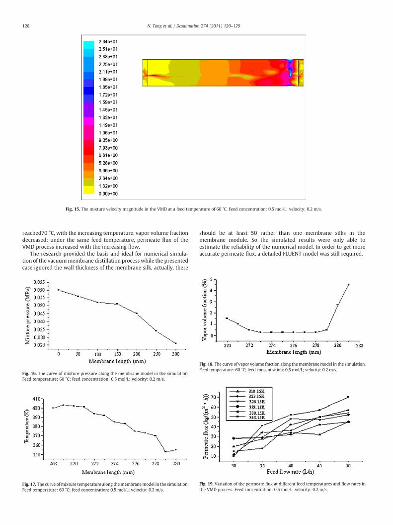
Fig. 15. The mixture velocity magnitude in the VMD at a feed temperature of 60 °C. Feed concentration: 0.5 mol/L; velocity: 0.2 m/s.
128 N. Tang et al. / Desalination 274 (2011) 120–129
reached70 °C, with the increasing temperature, vapor volume fractiondecreased; under the same feed temperature, permeate flux of theVMD process increased with the increasing flow.
The research provided the basis and ideal for numerical simula-tion of the vacuummembrane distillation process while the presentedcase ignored the wall thickness of the membrane silk, actually, there
Fig. 16. The curve of mixture pressure along the membrane model in the simulation.Feed temperature: 60 °C; feed concentration: 0.5 mol/L; velocity: 0.2 m/s.
Fig. 17. The curve ofmixture temperature along themembranemodel in the simulation.Feed temperature: 60 °C; feed concentration: 0.5 mol/L; velocity: 0.2 m/s.
should be at least 50 rather than one membrane silks in themembrane module. So the simulated results were only able toestimate the reliability of the numerical model. In order to get moreaccurate permeate flux, a detailed FLUENT model was still required.
Fig. 18. The curve of vapor volume fraction along themembranemodel in the simulation.Feed temperature: 60 °C; feed concentration: 0.5 mol/L; velocity: 0.2 m/s.
Fig. 19. Variation of the permeate flux at different feed temperatures and flow rates inthe VMD process. Feed concentration: 0.5 mol/L; velocity: 0.2 m/s.
129ation 274 (2011) 120–129
List of symbols
υm: mass-averaged velocity (m/s)ρm: mixture density (kg/m3)αk: volume fraction of phase kN: number of phasesκ: turbulence kinetic energy (J)ε: dissipation rate of κ(m2/s)→F: body force(N)μm: viscosity of the mixture (m/s)C: constant→υdr;k: drift velocity for secondary phase k (m/s)keff: effective conductivity [W/(m·K)]kt: turbulent thermal conductivity [W/(m·K)]hk: sensible enthalpy for phase k (J)Acknowledgements
This study was supported by Tianjin Science Planning Projectswith both (09ZCKFSH02600) and (2010CG11-02).
References
[1] Y.L. Wu, Membrane Science and Technology 23 (2003) 67–92.
N. Tang et al. / Desalin
[2] K. Smolders, A.C.M. Franken, Desalination 72 (1989) 249–262.[3] M. Liu, Application Manual of Membrane Separation Technology, Beijing Chemical
Industry Press, Beijing, 2001.[4] S. Kimura, S. Nakao, Journal of Membrane Science 33 (1987) 285–298.[5] F.J.Wang, Computational Fluid Dynamics, TsinghuaUniversity Press, Beijing, 2004.[6] Y. Yang, B.G. Wang, Y. Peng, Journal of Chemical Industry and Engineering 59
(2008) 1979–1985.[7] X.J. Qi, R. Tian, X.H. Yang, et al., Membrane Science and Technology 3 (2007) 35–39.[8] Z.Z. Han, J. Wang, D. Lan, FLUENT Simulation of Fluid Engineering Examples and
Applications, Beijing Institute of Technology Press, Beijing, 2004.[9] R.J. Wang, K. Zhang, G. Wang, FLUENT Technology Foundation and its Application,
Tsinghua University Press, Beijing, 2006.[10] Q. Wang, B. Maze, H.V. Tafreshi, et al., Modeling & Simulation in Materials Science
and Engineering 15 (2007) 855–868.[11] B.Maze,H.V. Tafreshi, B. Pourdeyhimi, Journal ofApplied Physics 102 (2007) 073533.[12] S. Jaganathan, H.V. Tafreshi, B. Pourdeyhimi, Powder Technology 181 (2008) 89–95.[13] S. Jaganathan, H.V. Tafreshi, B. Pourdeyhimi, Chemical Engineering Science 63
(2008) 244–252.[14] L. Spielman, S.L. Goren, Environmental Science and Technology 2 (1968) 279–287.[15] T. Hayat, M. Khan, S. Asghar, Acta Mechanica Sonica 23 (2007) 257–261.[16] H. Junqi, L. Ciqun, Science in China, Ser. A 26 (1996) 912–920.[17] M. Xu, W.C. Tan, Science in China, Ser. A 31 (2001) 626–638.[18] S.F. Chen, B.N. Sun, J.C. Tang, AppliedMathematics andMechanics 19 (1998) 95–100.[19] G.X. Li, R. Dirk, Progress in Natural Science 15 (2005) 458–462.[20] N. Tang, P.G. Cheng, X.K.Wang, et al., Chemical Engineering Transactions 17 (2009)
1537–1542.