1

Validation of a large area land cover product using purpose-1

acquired airborne video 2

3

M.A. Wulder*, J.C. White, S. Magnussen, S. McDonald 4

Canadian Forest Service (Pacific Forestry Centre), Natural Resources Canada, Victoria, 5 British Columbia, Canada 6 7 * Corresponding author: 8 506 West Burnside Rd., Victoria, BC V8Z 1M5; 9 Phone: 250-363-6090; Fax: 250-363-0775; Email: mike.wulder@pfc.cfs.nrcan.gc.ca 10 11 12 13 14 15 16 17 18 19 Pre-print of published version. 20

Reference: 21

Wulder, M.A., White, J.C., Magnussen, S., McDonald, S. 2007. Validation of large area 22 land cover product using purpose-acquired airborne video. Remote Sensing of 23 Environment, 106: 480–491. 24 25 DOI. 26

DOI: HUhttp://doi:10.1016/j.rse.2006.09.012U 27

28

Disclaimer: 29

The PDF document is a copy of the final version of this manuscript that was subsequently 30 accepted by the journal for publication. The paper has been through peer review, but it 31 has not been subject to any additional copy-editing or journal specific formatting (so will 32 look different from the final version of record, which may be accessed following the DOI 33 above depending on your access situation). 34

35 36

2

Abstract 37

38 Large area land cover products generated from remotely sensed data are difficult to 39 validate in a timely and cost effective manner. As a result, pre-existing data are often 40 used for validation. Temporal, spatial, and attribute differences between the land cover 41 product and pre-existing validation data can result in inconclusive depictions of map 42 accuracy. This approach may therefore misrepresent the true accuracy of the land cover 43 product, as well as the accuracy of the validation data, which is not assumed to be 44 without error. Hence, purpose-acquired validation data is preferred; however, logistical 45 constraints often preclude its use - especially for large area land cover products. Airborne 46 digital video provides a cost-effective tool for collecting purpose-acquired validation data 47 over large areas. An operational trial was conducted, involving the collection of airborne 48 video for the validation of a 31,000 square kilometre sub-sample of the Canadian large 49 area Earth Observation for Sustainable Development of Forests (EOSD) land cover map 50 (Vancouver Island, British Columbia, Canada). In this trial, one form of agreement 51 between the EOSD product and the airborne video data was defined as a match between 52 the mode land cover class of a 3 by 3 pixel neighbourhood surrounding the sample pixel 53 and the primary or secondary choice of land cover for the interpreted video. This scenario 54 produced the highest level of overall accuracy at 77% for level 4 of classification 55 hierarchy (13 classes). The coniferous treed class, which represented 71% of Vancouver 56 Island, had an estimated user's accuracy of 86%. Purpose acquired video was found to be 57 a useful and cost-effective data source for validation of the EOSD land cover product. 58 The impact of using multiple interpreters was also tested and documented. Improvements 59 to the sampling and response designs that emerged from this trial will benefit a full-scale 60 accuracy assessment of the EOSD product. 61 62 63 1.0 0BINTRODUCTION 64

The classification of land cover over large geographic areas with remotely sensed data is 65 increasingly common; regions (Homer et al., 1997), nations (Loveland et al., 1991; Fuller 66 et al., 1994; Cihlar and Beaubien, 1998), continents (Stone et al., 1994), and the globe 67 (Loveland and Belward, 1997; Loveland et al., 2000; Hansen et al., 2000) have been 68 mapped with a variety of satellite data types. This surge of interest in large area land 69 cover mapping projects may be explained by an increase in image availability, a need for 70 national- and global-scale land cover products for modelling and monitoring activities, 71 and political obligations related to international treaties such as the Convention on 72 Climate Change (Kyoto Protocol). Standard operational protocols for the validation of 73 these products are emerging (Loveland et al., 1999; Justice et al., 2000; Strahler et al., 74 2006; Wulder et al., 2006a), and a new initiative is addressing both the harmonization and 75 validation of large area land cover products (Herold et al., 2006). 76 77 A sufficient level of accuracy is assumed in order to rationalize the applied use of these 78 large area land cover products for a wide variety of applications (Morisette et al., 2002; 79 Stehman and Czaplewski, 2003). Accuracy assessment protocols require validation data 80 that is independent from information used in map development; however, validation data 81

3

is expensive and logistically challenging to collect for large area land cover products 82 (Cihlar, 2000). As a result, pre-existing data are often used for validation of large area 83 land cover products generated from remotely sensed data. Unfortunately, temporal, 84 spatial, and attribute differences between the land cover product and the pre-existing 85 validation data can result in poor levels of apparent accuracy (Remmel et al., 2005). 86 Furthermore, the use of pre-existing validation data may misrepresent the true accuracy 87 of the land cover product, while at the same time, revealing problems inherent in the 88 validation data. Aerial videography is one means of collecting purpose-acquired 89 validation data for land cover products extending over large areas (Slaymaker, 2003). 90 91 Airborne videography became known as a flexible and cost effective remote sensing tool 92 in the early 1980s (Meisner, 1986; Mausel et al., 1992; King, 1995), and has 93 demonstrated utility for a wide range of applications including species identification and 94 vegetation mapping (Nixon et al., 1985; Bobbe et al., 1993; Frazier, 1998; Suzuki et al., 95 2004), forest health and damage assessment (Jacobs and Eggen-McIntosh, 1993; Jacobs, 96 2000); forest inventory update (Brownlie et al., 1996; Davis et al., 2002); and validation 97 of vegetation maps generated from medium resolution remotely sensed data (Graham, 98 1993; Marsh et al., 1994; Slaymaker et al., 1996; Hepinstall, 1999; Hess et al., 2002). 99 Marsh et al. (1994) compared the use of systematically acquired aerial colour 100 photography and airborne video for the validation of land cover products generated from 101 Landsat TM imagery. The similarity between the accuracies measured by the 102 photography and video sources was statistically significant (α = 0.01), suggesting that 103 video could provide validation data of similar quality and utility to that of traditional 104 aerial photography, with the advantage of collecting a larger volume of data with the 105 same level of effort. 106 107 Aerial videography gained additional momentum in the 1990s as a result of the GAP 108 analysis programs implemented in the United States (Slaymaker, 2003). GAP programs 109 operated at the state level and were initiated to assess the extent to which native animal 110 and plant species were being protected. GAP land cover maps generated from Landsat 111 TM data required a source of calibration data to facilitate the classification of the 112 imagery, as well as a source of validation data to assess the accuracy of the output 113 vegetation maps (Scott et al., 1993; Slaymaker, 2003). Aerial point sampling methods 114 developed by Norton-Griffiths (1982) for aerial photography were adapted to aerial 115 videography by Graham (1993) and implemented in the Arizona GAP program. The 116 automatic labelling of video frames with Global Positioning System (GPS) coordinates 117 was a major technological advancement, "providing a way to precisely and automatically 118 match video-recorded GPS time with the position information in the GPS data file" 119 (Graham, 1993: 29). Slaymaker et al. (1996) modified this approach for the GAP 120 program in New England. Aerial video for calibration and validation of Landsat-based 121 land cover maps was subsequently adopted by many other state-wide GAP programs 122 (Schlagel, 1995; Driese et al., 1997; Hepinstall et al., 1999; Reiners et al., 2000), as well 123 as for other land cover products (Skirvin et al., 2000; Hess et al., 2002; Maingi et al., 124 2002; Skirvin et al., 2004). Technological advances in the 1990s led to the development 125 of digital video cameras and powerful multi-media capabilities in desktop computers, 126 further enhancing the quality and affordability of video options (Hess et al. 2002) 127

4

128 The advantages and disadvantages of airborne video for validation of land cover maps are 129 summarized in Slaymaker (2003). One of the main advantages of video is data 130 redundancy (Mausel et al. 1992), which facilitates the collection of large samples of 131 validation (and calibration) points at specified intervals (of time or distance). In the early 132 1990s, the inferior resolution of video (240 lines for colour, 300 lines for panchromatic) 133 compared to that of 35 mm photo film (1500 lines) was an impediment to the widespread 134 adoption of video for land cover applications (Slaymaker, 2003). Since this time, the 135 quality of video has improved dramatically; with current consumer grade digital video 136 cameras typically having more than 500 lines (colour) (Jack, 2005). 137 138 The main goal of the Earth Observation for Sustainable Development of Forests (EOSD) 139 program is the creation of a land cover map of the forested area of Canada, produced to 140 represent year 2000 conditions, and on track for completion in 2006 (Wulder et al. 2003). 141 There are many areas in the north of Canada being mapped for the EOSD project that are 142 inaccessible, have no pre-existing detailed forest or vegetation inventories, and minimal 143 or out-dated aerial photography. While a framework for validating the EOSD product has 144 been developed (Wulder et al., 2006a), an alternative data source, along with a protocol 145 for using this data source to validate the EOSD product, is required. The objective of this 146 study was to develop a protocol and demonstrate the use of airborne video as a source of 147 validation data for large area land cover products generated from remotely sensed data, 148 specifically the EOSD land cover product. The rationale and approaches demonstrated 149 here are intended to be portable to other large area mapping programs. 150 151 To fully explore the potential of airborne video for validation of the EOSD product, an 152 operational trial was conducted on Vancouver Island, British Columbia, Canada. Video 153 data was used for validation and the accuracy estimates were compared to the estimates 154 obtained using pre-existing forest inventory data for validation. Pre-existing data is often 155 considered a viable source of validation data, despite fundamental differences that often 156 exist between the pre-existing data and the product being validated. This communication 157 details the protocol developed through this operational trial, the results of the accuracy 158 assessment using the airborne video, the impact of multiple interpreters, and suggested 159 improvements for future implementation of the video system for validation. 160 161 162 2.0 1BSTUDY AREA 163 164 Vancouver Island has a total land area of 31,284 square kilometres (Figure 1). Much of 165 the island (85%) lies in the Coastal Western Hemlock biogeoclimatic zone (Klinka et al. 166 1991). This zone is characterized as one of Canada's wettest climates and most productive 167 forest areas, with cool summers and mild winters. The rugged physical features of 168 Vancouver Island include long mountain-draped fjords on the west coast, coastal plains 169 on the eastern coast, and a chain of glaciated mountains running along the north-south 170 axis of the Island. Elevations range from 0 to 2200 metres. Forests cover 91% of 171 Vancouver Island and forest species, in order of prevalence, include Hemlock (Tsuga 172 spp.), Western red cedar (Thuja plicata Donn ex. Don), Western hemlock (Tsuga 173

5

heterophylla (Raf.) Sarg.), Yellow cedar (Chamaecyparis nootkatensis (D. Don) Spach.), 174 and Douglas-fir (Pseudotsuga menziesii (Mirb.) Franco). The existing forest inventory 175 indicates that approximately 45% of the forest on the island is 250 years in age or older, 176 with the remaining forest in managed second-growth stands. 177 178 179

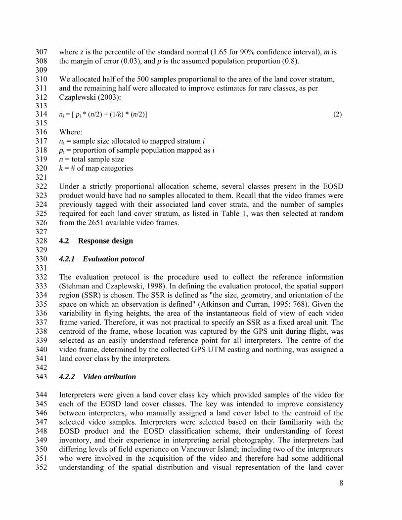
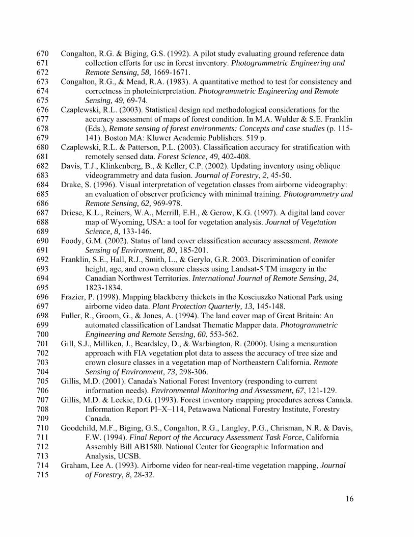
3.0 2BDATA 180 181 3.1 8BEarth Observation for Sustainable Development of Forests (EOSD) 182 183 In support of meeting national and international monitoring and reporting commitments, 184 the Canadian Forest Service, in partnership with the Canadian Space Agency, is 185 classifying Landsat data over the forested area of Canada. Over 400 Landsat scenes are 186 being used to map the approximately 400 million hectares of treed land present in Canada 187 (Wulder and Seemann 2001), with 20 different land cover classes (plus additional classes 188 for no data, shadow, and cloud) (Wulder and Nelson, 2003) as listed in Table 1. Including 189 image overlap into non-forest areas, over 60% of the country will be mapped by the 190 EOSD project, with image classification undertaken by federal, provincial, and territorial 191 agencies (Wulder et al. 2003). Source images cover acquisition dates ranging from 1999 192 to 2002 and the EOSD product has a pixel size of 25 metres. 193 194 The land cover classification system used for the EOSD product is based on the 195 classification system originally developed for the National Forest Inventory (NFI) 196 program. The six levels of the NFI classification hierarchy include vegetation cover, tree 197 cover, landscape position, vegetation type, forest density, and species diversity (Figure 2; 198 Gillis, 2001). The EOSD classification hierarchy is identical in principle, but is limited to 199 a level of detail discernable in Landsat imagery (Wulder and Nelson, 2003; Wulder et al. 200 2003). Thus, Levels 3 (landscape position) and 6 (species diversity) are not included. 201 Using the NFI class structure as a base, level 4 (vegetation type), along with level 5 forest 202 density descriptors, the closed legend in Figure 2 emerged. Building upon the existing 203 NFI hierarchy enables classification and class generalization. The generalization or 204 collapsing of classes can be useful for reporting validation results for different levels of 205 classification detail, thereby accommodating a wider range of end-users. The EOSD-NFI 206 legend has been cross-walked to a number of regional, national, and international land 207 cover legends (Wulder and Nelson, 2003) augmenting the utility of the land cover 208 products generated. 209 210 3.2 9BForest inventory 211 212 Existing provincial forest inventory data were available in digital format in a GIS 213 database for approximately 26,000 square kilometres of Vancouver Island; inventory 214 information was not available for areas not subject to inventory activities, including parks 215 and private lands. The inventory is the primary source of information on the distribution 216 and areal extent of forest stands, logging roads, and past natural and human disturbances 217 in the study region. The inventory includes species composition (of up to six species, 218

6

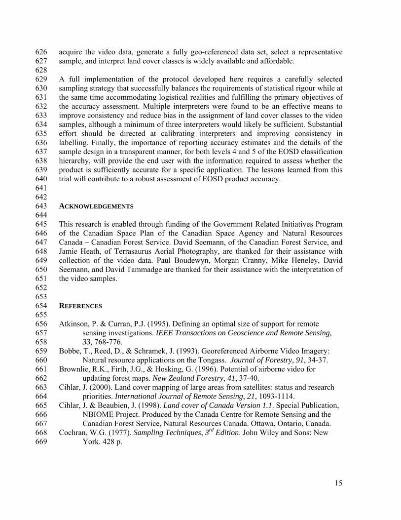
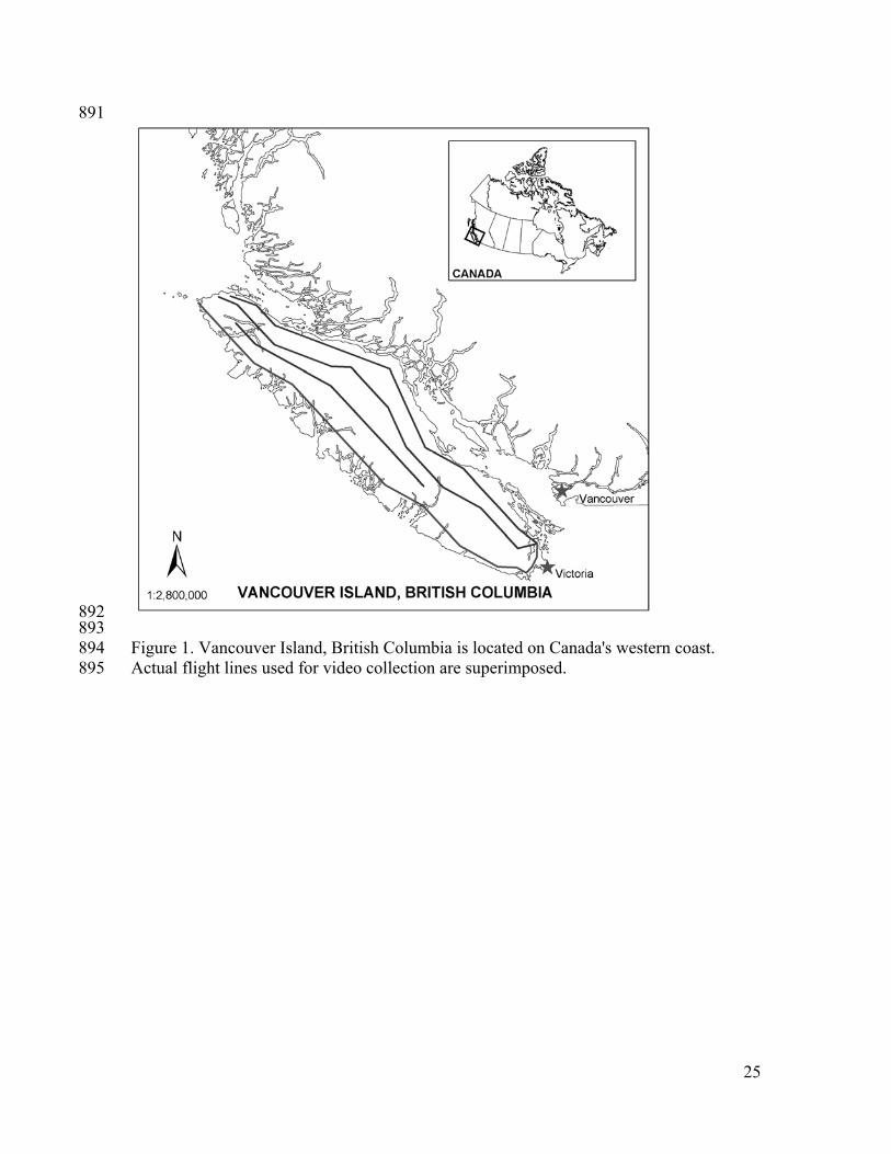
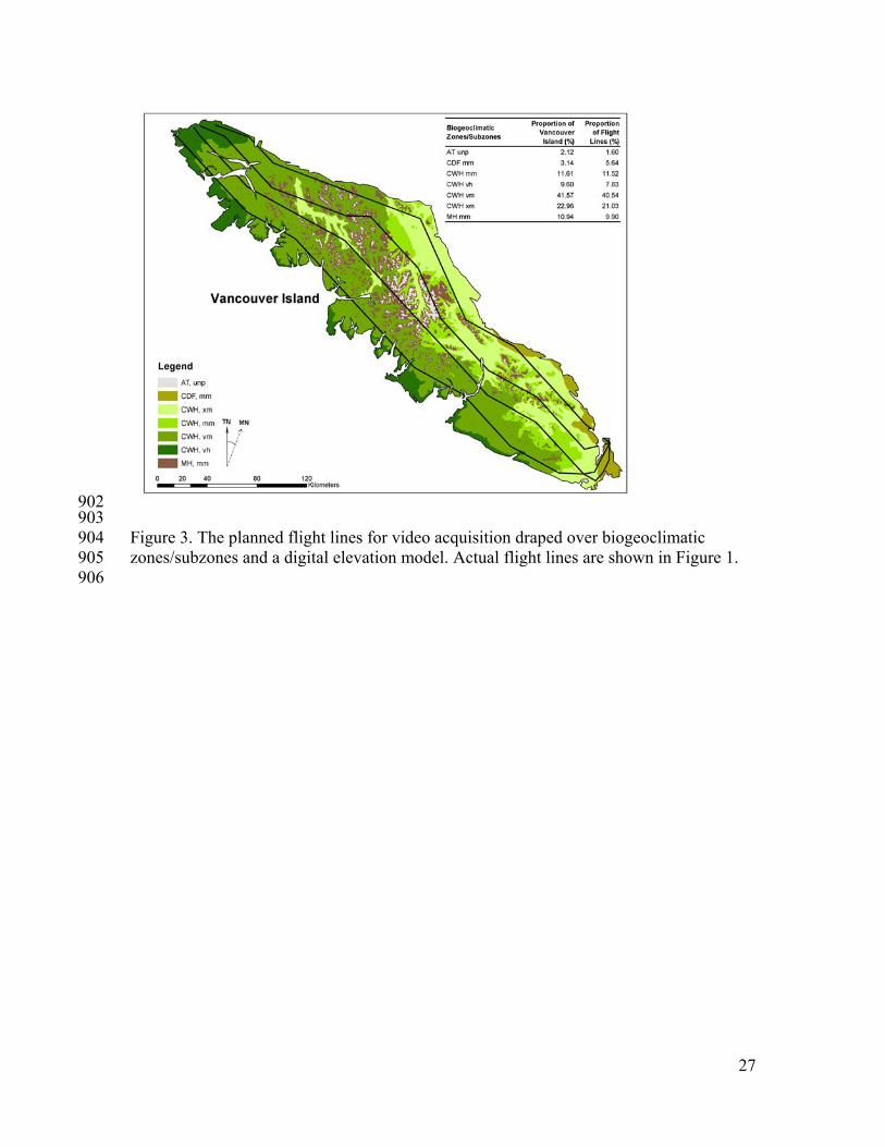
with estimates of species prevalence to the nearest 10%), stand age in years, crown 219 closure (to the nearest 5%), stand height in metres, diameter at breast height in 220 centimetres, and stand area in hectares (Gillis and Leckie, 1993). Some stands were 221 labelled non-productive forest. Much of the inventory information was projected to 222 represent 1999 forest conditions; the original data collection reference years for 223 individual stands ranged from 1954 to 1999. A method was developed for this study to 224 generate EOSD-equivalent labels from attributes in the forest inventory using various 225 combinations of species and species composition, age, crown closure, height, and non-226 productive forest codes. As a result, each forest inventory polygon was assigned an 227 EOSD land cover label. 228 229 3.3 10BAirborne video 230 231 The equipment used to collect the video data consisted of a Sony™ DCR-PC330 digital 232 camcorder and a Red Hen A-VMS 300 device. The Red Hen (Red Hen Systems, Fort 233 Collins, Colorado, USA) device included a Thales™ B12 GPS engine (a real-time 234 differential GPS (DGPS) receiver), which is horizontally accurate to within 3 metres, and 235 is used to encode/decode GPS positional information onto the audio track of the video 236 recording. The Sony™ DCR-PC330 is a MiniDV format camcorder that is compact and 237 lightweight, with 530 lines of resolution and a single Advanced HAD™ 1/3" CCD with 238 3310K total pixels. The effective video resolution is 2048K pixels. The video camera and 239 Red Hen device were mounted in a Cessna 206 aircraft, which had a 12-inch photo port 240 on its underside. Due to the highly variable topography on Vancouver Island, and 241 associated difficulties in maintaining a consistent flying height, the scale of the video 242 ranged from 1:500 to 1:30000, with pixel sizes on the ground ranging from 1 cm to 60 cm 243 and frame extents from 2.4 by 1.8 m to 144 by 108 m. Four flight lines, extending the full 244 length of Vancouver Island, were flown over a two day period on August 10th and 11th 245 2004, resulting in approximately 11 hours of continuous video (Figure 1), representing 246 approximately 0.5% of the land area of Vancouver Island. The flight lines were designed 247 to capture the greatest range of land cover classes possible. Ancillary data such as 248 biogeoclimatic zones and base planimetric layers were compiled and referenced when the 249 flight plan was being developed. The average flying height above the terrain, was 585 250 metres; however, flying heights varied in areas of steep topography. Post-flight, the video 251 and GPS information were integrated to create a completely digital and fully 252 georeferenced record of the flight lines using the Red Hen MediaMapper® software. 253 254 255

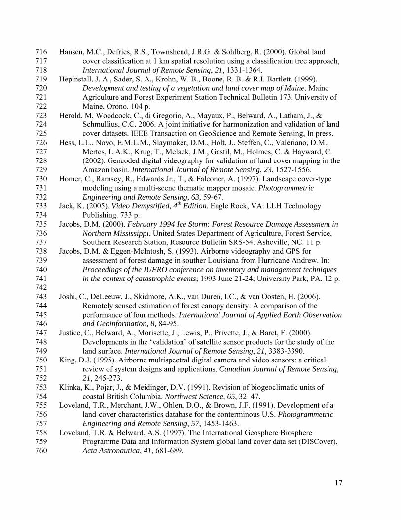
4.0 3BMETHODS 256 257 4.1 11BSampling design 258 259 A two-phase sampling design was used, with the first phase being the collection of the 260 airborne video, followed by post-stratification of the video samples by the EOSD land 261 cover strata. The sample frame for the study was the contiguous landmass of Vancouver 262 Island (Figure 1). At the time the video acquisition was being planned, the EOSD product 263

7

for Vancouver Island was not complete, and the spatial distribution of the EOSD land 264 cover classes was not known. Given limited resources for flying and video acquisition, a 265 surrogate source of ecological mapping was used to ensure the flight lines were 266 ecologically representative and that sufficient numbers of samples could be collected for 267 all possible land cover classes. To achieve this, biogeoclimatic ecosystem zones and 268 subzones, combined with a digital elevation model, were used to guide the placement of 269 flight lines (Figure 3). Biogeoclimatic ecosystem subzones represent unique sequences of 270 geographically related ecosystems, which are grouped into broader biogeoclimatic zones, 271 of which there are four unique zones on Vancouver Island (Meidinger and Pojar, 1991). 272 The table included in Figure 3 indicates that the flight lines characterized the spatial 273 distribution of biogeoclimatic zone/subzone combinations. Although the flight lines were 274 not selected via a probability sampling design, the resulting sample is assumed to be 275 representative of the land cover distribution of Vancouver Island. Individual video frames 276 were extracted at 15 second intervals, resulting in a total of 2651 possible frames, from 277 all of the flight lines. Each video frame was assigned a unique identifier. Points 278 representing the centroid locations of these video frames were overlaid with the EOSD 279 product to derive the corresponding EOSD land cover class for the video frame in order 280 to facilitate proportional allocation of the sample units to the EOSD land cover strata. The 281 individual video frames were then pooled (i.e., no longer associated with their source 282 transect) and sorted randomly. 283 284 4.1.1 20BSample size 285 286 The selection of sample size often involves tradeoffs between the requirements of 287 statistical rigour and logistical realities. The objective of this study was to develop a 288 protocol for the use of video for validation, and one of the key issues requiring 289 exploration was the necessary number of interpreters to assign land cover attributes to the 290 video frames. The assumption was that the greater the number of interpreters, the less 291 subjective the interpretation was likely to be (since the mode of all seven interpreters 292 would be compared to the EOSD product label). Seven interpreters familiar with EOSD 293 and vegetation on Vancouver Island were selected. Sufficient resources were not 294 available for the seven interpreters to label all 2651 video frames that were collected, and 295 therefore a subset of video frames had to be selected. The sample had to be large enough 296 to facilitate statistical testing and provide confidence in the overall accuracy estimate, 297 while at the same time ensuring each land cover class had sufficient samples for reporting 298 user's and producer's accuracies (Czaplewski and Patterson, 2003). 299 300 An overall sample size of approximately 500 was determined by specifying a 90% 301 confidence interval for p with a margin of error of 0.03, and an assumption of 80% true 302 accuracy (Cochran, 1977): 303 304

2

(1 )z

n p pm

(1) 305

306

8

where z is the percentile of the standard normal (1.65 for 90% confidence interval), m is 307 the margin of error (0.03), and p is the assumed population proportion (0.8). 308 309 We allocated half of the 500 samples proportional to the area of the land cover stratum, 310 and the remaining half were allocated to improve estimates for rare classes, as per 311 Czaplewski (2003): 312 313 ni = [ pi * (n/2) + (1/k) * (n/2)] (2) 314 315 Where: 316 ni = sample size allocated to mapped stratum i 317 pi = proportion of sample population mapped as i 318 n = total sample size 319 k = # of map categories 320 321 Under a strictly proportional allocation scheme, several classes present in the EOSD 322 product would have had no samples allocated to them. Recall that the video frames were 323 previously tagged with their associated land cover strata, and the number of samples 324 required for each land cover stratum, as listed in Table 1, was then selected at random 325 from the 2651 available video frames. 326

327 4.2 12BResponse design 328 329 4.2.1 21BEvaluation potocol 330 331 The evaluation protocol is the procedure used to collect the reference information 332 (Stehman and Czaplewski, 1998). In defining the evaluation protocol, the spatial support 333 region (SSR) is chosen. The SSR is defined as "the size, geometry, and orientation of the 334 space on which an observation is defined" (Atkinson and Curran, 1995: 768). Given the 335 variability in flying heights, the area of the instantaneous field of view of each video 336 frame varied. Therefore, it was not practical to specify an SSR as a fixed areal unit. The 337 centroid of the frame, whose location was captured by the GPS unit during flight, was 338 selected as an easily understood reference point for all interpreters. The centre of the 339 video frame, determined by the collected GPS UTM easting and northing, was assigned a 340 land cover class by the interpreters. 341 342 4.2.2 22BVideo atribution 343

Interpreters were given a land cover class key which provided samples of the video for 344 each of the EOSD land cover classes. The key was intended to improve consistency 345 between interpreters, who manually assigned a land cover label to the centroid of the 346 selected video samples. Interpreters were selected based on their familiarity with the 347 EOSD product and the EOSD classification scheme, their understanding of forest 348 inventory, and their experience in interpreting aerial photography. The interpreters had 349 differing levels of field experience on Vancouver Island; including two of the interpreters 350 who were involved in the acquisition of the video and therefore had some additional 351 understanding of the spatial distribution and visual representation of the land cover 352

9

classes. Strand et al. (2002) demonstrated that direct field experience did not improve the 353 accuracy with which photo interpreters could label land cover types; however, Drake 354 (1996) demonstrated that even a minimum amount of training can improve the 355 interpretation of vegetation classes from airborne video. 356 357 The key points communicated to the interpreters included (Wulder et al., 2004): 358 Tall and low shrubs would be grouped into a single shrub class. 359 Density classes, particularly the distinction between dense and open classes, are 360

known to be problematic. Interpreters were advised when not certain of the density 361 class to select both a primary and secondary class label (e.g. primary label: dense 362 conifer, secondary label: open conifer). 363

Guidelines for defining mixed wood stands were provided (i.e., when neither 364 coniferous nor broadleaf species account for more than 75% of the total basal area 365 in the stand). 366

Several examples of video frames were provided for each land cover class to 367 promote consistent interpretations. 368

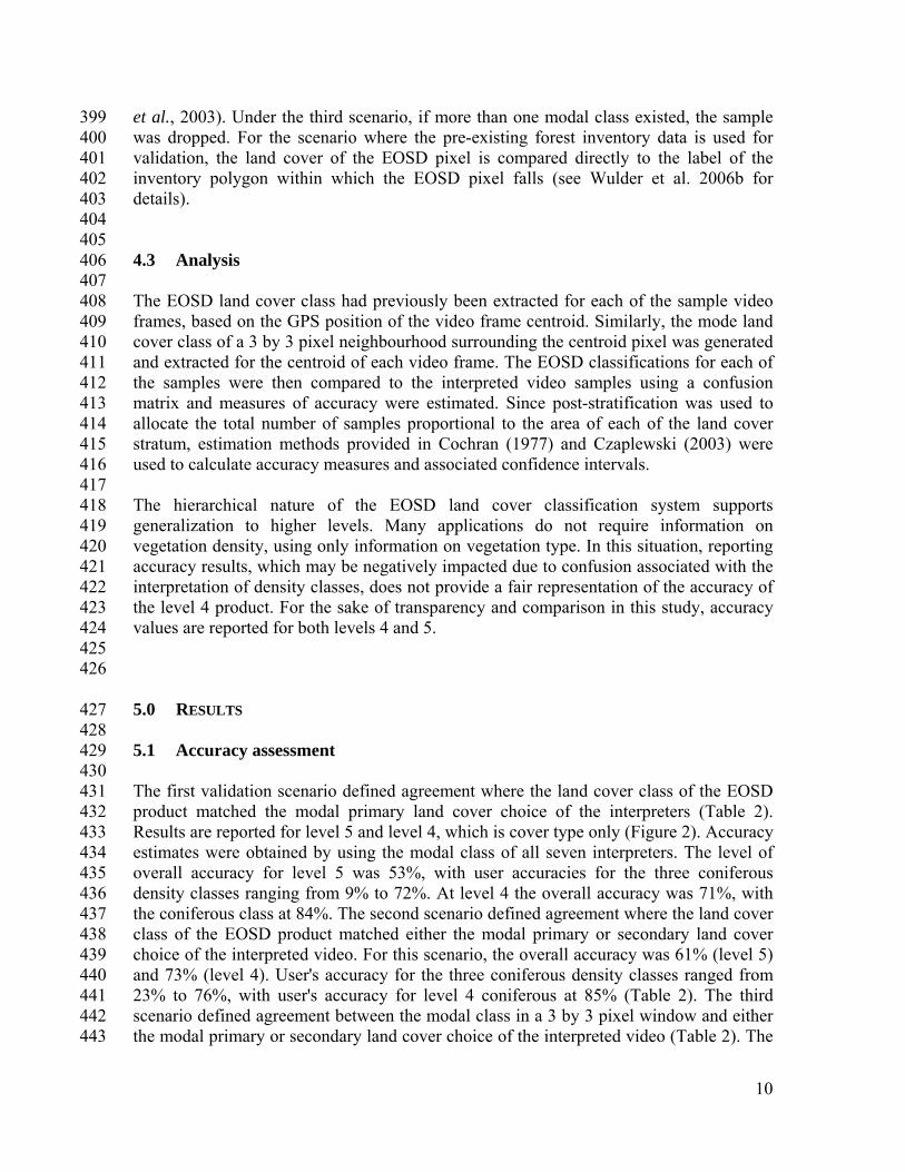
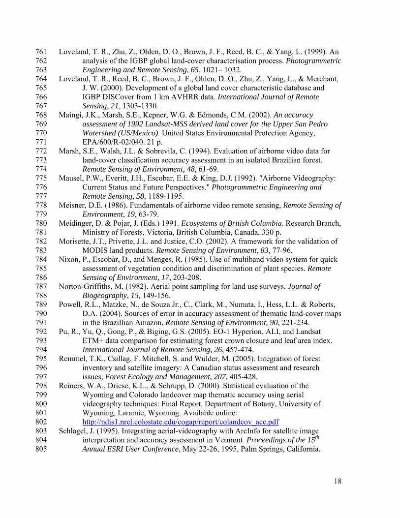
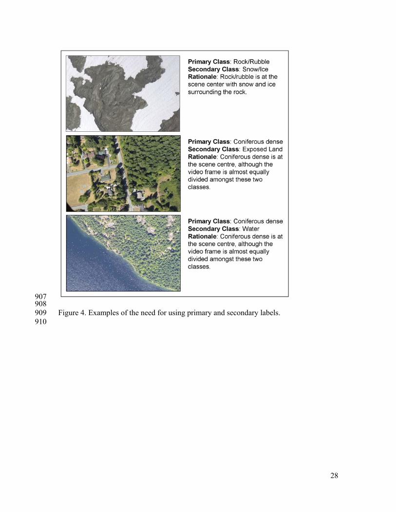
369 4.2.3 23BLabelling protocol 370 371 The interpreters were provided with a listing of the sample video frames. Recall that the 372 sample video frames had been pooled and sorted randomly by their unique identifier. The 373 interpreters did not know the geographic location of the video frame, or the flight line 374 that the video frame originated from. The interpreters were also not privy to the EOSD 375 land cover stratum from which the video frame was selected. Each interpreter 376 independently determined an appropriate label for the land cover type existing at the 377 centre of the video frame. As per Stehman et al. (2003), the interpreters selected the most 378 likely class (primary choice) with an option to specify a second choice if necessary. The 379 secondary choice captures the confusion between classes when the frame falls in the 380 transition between two cover-type classes (Figure 4), thereby acknowledging thematic 381 and non-thematic errors (Foody, 2002). 382 383 4.2.4 24BDefining agreement 384 385 Several scenarios for defining agreement between the EOSD product and the interpreted 386 video frames were explored: 387

1. If the land cover class of the EOSD product matched the primary land cover choice 388 of the interpreted video. 389

2. If the land cover class of the EOSD product matched either the primary or 390 secondary land cover choice of the interpreted video. 391

3. If the modal class of a 3 by 3 pixel SSR around the target EOSD pixel matched 392 either the primary or secondary land cover choice of the interpreted video. 393

394 The first scenario is a direct comparison between the interpreted video and the EOSD 395 product, making no allowances for possible errors in attribution and/or positional 396 accuracy. The second scenario listed above accommodates thematic ambiguity, while the 397 third choice accommodates both thematic ambiguity and positional uncertainty (Stehman 398

10

et al., 2003). Under the third scenario, if more than one modal class existed, the sample 399 was dropped. For the scenario where the pre-existing forest inventory data is used for 400 validation, the land cover of the EOSD pixel is compared directly to the label of the 401 inventory polygon within which the EOSD pixel falls (see Wulder et al. 2006b for 402 details). 403 404 405 4.3 13BAnalysis 406 407 The EOSD land cover class had previously been extracted for each of the sample video 408 frames, based on the GPS position of the video frame centroid. Similarly, the mode land 409 cover class of a 3 by 3 pixel neighbourhood surrounding the centroid pixel was generated 410 and extracted for the centroid of each video frame. The EOSD classifications for each of 411 the samples were then compared to the interpreted video samples using a confusion 412 matrix and measures of accuracy were estimated. Since post-stratification was used to 413 allocate the total number of samples proportional to the area of each of the land cover 414 stratum, estimation methods provided in Cochran (1977) and Czaplewski (2003) were 415 used to calculate accuracy measures and associated confidence intervals. 416 417 The hierarchical nature of the EOSD land cover classification system supports 418 generalization to higher levels. Many applications do not require information on 419 vegetation density, using only information on vegetation type. In this situation, reporting 420 accuracy results, which may be negatively impacted due to confusion associated with the 421 interpretation of density classes, does not provide a fair representation of the accuracy of 422 the level 4 product. For the sake of transparency and comparison in this study, accuracy 423 values are reported for both levels 4 and 5. 424 425 426

5.0 4BRESULTS 427 428 5.1 14BAccuracy assessment 429 430 The first validation scenario defined agreement where the land cover class of the EOSD 431 product matched the modal primary land cover choice of the interpreters (Table 2). 432 Results are reported for level 5 and level 4, which is cover type only (Figure 2). Accuracy 433 estimates were obtained by using the modal class of all seven interpreters. The level of 434 overall accuracy for level 5 was 53%, with user accuracies for the three coniferous 435 density classes ranging from 9% to 72%. At level 4 the overall accuracy was 71%, with 436 the coniferous class at 84%. The second scenario defined agreement where the land cover 437 class of the EOSD product matched either the modal primary or secondary land cover 438 choice of the interpreted video. For this scenario, the overall accuracy was 61% (level 5) 439 and 73% (level 4). User's accuracy for the three coniferous density classes ranged from 440 23% to 76%, with user's accuracy for level 4 coniferous at 85% (Table 2). The third 441 scenario defined agreement between the modal class in a 3 by 3 pixel window and either 442 the modal primary or secondary land cover choice of the interpreted video (Table 2). The 443

11

overall accuracy for this scenario was 67% for level 5 and 76% for level 4. User's 444 accuracies for the three coniferous density classes ranged from 15% to 82%, and the 445 user's accuracy for the coniferous class was 86%. With pre-existing forest inventory data 446 used as reference data the overall accuracy was 41% for level 5 and 68% for level 4. 447 User's accuracies for the coniferous density classes ranged from 0% to 55% and the user's 448 accuracy for the coniferous class was 74%. 449 450 5.2 15BMultiple interpreters 451 452 A summary of overall accuracy, as estimated by each interpreter for each scenario, is 453 provided in Table 3. These results provide an indication of what the accuracy estimates 454 would have been if only one interpreter had been used for the project. Overall accuracies 455 varied by an average of 8% for level 5 and 11% for level 4. Pairwise comparisons for 456 each scenario were made between interpreters, and between interpreters and the EOSD 457 product, and the proportion of agreement is summarized in Table 4. 458 459 460 6.0 5BDISCUSSION 461

6.1 16BUse of purpose-acquired video for validation 462 463 There are a number of issues to consider when determining the appropriateness of video 464 data for an accuracy assessment. Video can cover large geographic areas efficiently, and 465 areas that are identified in the flight plan as unique or rare can be sampled intensively. 466 When compared to field surveys, video facilitates the collection of a large number of 467 sampling locations, providing sufficient samples for both calibration and validation, and 468 the data redundancy and ability to view transitions between land cover classes can be 469 advantageous. Video also provides a permanent record of the survey and interpretation 470 may be done by highly trained professionals, mobilized at minimal cost, who have 471 extensive experience in identifying vegetation types and land cover from airborne 472 imagery. Technology has created advances in digital video that have resulted in higher 473 quality, compact cameras at increasingly affordable prices, and since there is little post-474 processing required, the data can be available almost immediately after collection. 475 Furthermore, sophisticated and readily available off-the-shelf software and hardware 476 products can generate video that is fully georeferenced, facilitating sampling protocols. 477 Digital photography has experienced similar advances in technology and reductions in 478 cost. Video acquisition must be planned so that the video meets the level of detail 479 required by the classification system, and flying height and speed must be set 480 accordingly. The efficiency, simplicity, and cost effectiveness of video make it an 481 attractive source of calibration and validation data for large area land cover products 482 generated from remotely sensed data. 483 484 The results of the accuracy assessment using the video frames for validation highlighted 485 several issues. First, accommodating positional and thematic ambiguity can have an 486 impact on the reported accuracy results (75% overall accuracy when these sources of 487 ambiguity are addressed versus 53% when they are not). Second, density classes were a 488

12

major source of classification confusion and result in low accuracy measures at level 5 of 489 the EOSD classification hierarchy. This may misrepresent the accuracy of the product to 490 end users who do not require information on vegetation density. Therefore, separate 491 accuracy estimates should be reported for both level 4 and level 5 land cover products, 492 allowing an end user to make informed decisions about the application-specific relevance 493 of each estimate. End users must also understand the limitations of the agreement 494 scenarios, and of accuracies reported for a generalized product (e.g., the mode of 3 by 3 495 pixel neighbourhood) (Czaplewski, 2003). Confusion between density classes also 496 suggests that greater effort is required to calibrate interpreters. Crown closure has been 497 identified as one of the more difficult forest inventory attributes to estimate or even 498 measure accurately (on the ground, from the air, or from satellite imagery) (Congalton 499 and Biging, 1992; Gill et al. 2000). The potential of extracting estimates of crown closure 500 from Landsat imagery has been the subject of ongoing research (e.g., Franklin et al., 501 2003; Xu et al., 2003; Pu et al., 2005; Joshi et al., 2006). 502 503 6.2 17BPre-existing forest inventory 504 505 The use of the pre-existing forest inventory as a source of validation data produced 506 overall accuracy results that were lower than the results produced using the purpose 507 acquired video for validation. For level 5, using the forest inventory data produced an 508 estimate of overall accuracy that ranged from 12% to 26% lower than that produced using 509 the video. Individual user's accuracies for the coniferous open class were similar, ranging 510 from 17% to 27% lower than the estimates associated with the video. At level 4, the 511 differences between the inventory and the video estimates of overall accuracy are not as 512 disparate, with the inventory estimating overall accuracy ranging from 3% to 9% lower 513 than the video estimates, and user's accuracies for the coniferous class that were 10% to 514 12% lower than that estimated from the video. Wulder et al. (2006b) document the 515 challenges of using pre-existing data (specifically forest inventory) to validate land cover 516 products generated from remotely sensed data: geolocational mismatches, differences in 517 features or classes mapped, disparity between the scale of polygon delineation and the 518 spatial resolution of the image, and temporal discrepancies. However, the greatest 519 challenge to using pre-existing data such as forest inventory for validation is that a forest 520 inventory polygon is a generalization, designed to represent areas of relatively 521 homogenous forest characteristics. In contrast, the raster based land cover product can 522 contain much more detail and is, by its very nature, heterogeneous, with a minimum 523 mapping unit (MMU) that often reflects the size of the image pixels (e.g., 0.06 ha) versus 524 the 2 ha MMU of the forest inventory. 525 526 6.3 18BMultiple interpreters 527 528 All of the seven interpreters' primary labels agreed only 20% of the time and of these, 529 36% were classed as not interpretable; 26% were open coniferous; and 22% were snow 530 and ice. This low level of agreement amongst the interpreters' primary label suggests 531 there was either ambiguity in the application of the classification legend or confusion 532 regarding the sample unit (i.e., the dominant land cover class for the frame as a whole 533 versus just the cover type located at the centroid of the chip). In 80% of the cases where 534

13

the interpreters' primary labels did not agree, 66% were attributed to disagreements over 535 density classes. Reporting accuracy estimates for level 4 of the EOSD hierarchy 536 eliminated this type of disagreement and increased interpreter agreement to 43% 537 (compared to 20% at level 5). 538 539 One of the drawbacks to using aerial photography or video for validation is the lack of 540 direct physical contact with the target (Congalton and Biging, 1992), therefore the 541 classification is still based on remote interpretation (albeit with a well established and 542 rigorous process). As such, there is no "truth", as multiple interpreters are unlikely to 543 agree 100% of the time. The absence of an absolute truth dataset makes it difficult to 544 assess the performance of any one interpreter, and to determine the optimal number of 545 interpreters required to provide an unbiased result. Powell et al., (2004) manufactured a 546 truth standard by having all five interpreters assign pixels to land cover classes by 547 consensus. The result was termed the "gold standard" and was used for the final accuracy 548 assessment. Powell et al., (2004) attributed some of the disagreement between 549 interpreters to human error (e.g., misinterpretation of the image printout, miscoding the 550 sample), while other disagreements related more fundamentally to identification of the 551 vegetation in the video. 552 553 Table 3 summarizes the overall accuracies for each scenario, by interpreter. If any one of 554 these interpreters had individually been selected to interpret the video, the overall 555 estimates of accuracy would have varied by an average of 8% for level 5 and 11% for 556 level 4. This result contrasts with that of Drake (1996) who concluded that individual 557 interpreters could be used to produce similar accuracy estimates, with little effect. Table 4 558 summarizes the overall proportion of agreement between interpreters and between 559 interpreters and the EOSD product. The results indicate that there was more agreement 560 amongst individual interpreters than there was between individual interpreters and the 561 EOSD product. For level 5, agreement between primary labels of any two interpreters 562 ranged by 20%, with an average overall agreement of 60%. If both the primary or 563 secondary label are considered, agreement between any two interpreters ranged by 23%, 564 with an average overall agreement of 77% and the highest agreement at 90%. 565 Comparisons between individual interpreters and the EOSD output were markedly lower. 566 If only the primary label of a single interpreter is considered, then overall agreement 567 averaged 40% (range 8%). If both primary and secondary label are compared to the 568 modal land cover class of a 3 by 3 pixel neighbourhood, overall agreement increased to 569 45% (range 9%). For level 4, the patterns in accuracy estimates are similar. Agreement 570 amongst interpreters was greater at more generalized levels of the EOSD hierarchy (70% 571 at level 4 versus 60% at level 5), and if thematic ambiguity was accounted for (77% for 572 both primary and secondary labels at level 5 versus 60% for primary label only at level 573 5). 574 575 These results suggest that the use of multiple interpreters can be important for reducing 576 bias and improving consistency in class labeling. The number of interpreters required 577 likely varies by application and depends on the complexity of the land cover classes. For 578 the method whereby the modal class of interpreters is used, a minimum of three 579 interpreters would be practical, and is recommended. An evaluation protocol that 580

14

incorporates independent classification by each interpreter, followed by cross calibration, 581 and revisit of problematic classes would be the most effective way to use fewer 582 interpreters (and fewer resources), while still taking advantage of the benefits of multiple 583 interpreters. 584 585 6.4 19BLessons learned 586 587 The main objective of this study was to develop a protocol and demonstrate the use of 588 airborne video as a source of validation data for large area land cover products, 589 specifically the EOSD. Over the course of conducting this operational trial, several issues 590 arose, providing opportunities to improve upon the methodology for future 591 implementation. First, a fully probabilistic sample design is clearly more important than 592 the representation of all potential classes – particularly since resources for the accuracy 593 assessment are scarce and a key objective of the EOSD accuracy assessment is to 594 generate robust estimates of overall accuracy and producer's and user's accuracies for the 595 dominant forest classes. To that end, flight lines should be placed so that they traverse the 596 study area at fixed intervals of distance in both north-south and east-west orientations. 597 Samples should be allocated proportional to strata area, with no accounting for rare 598 classes that have a very limited spatial extent. The video camera should be set to a fixed 599 zoom, facilitating an increase in the consistency of the scale of video frames. In addition, 600 the pilot should be instructed to try to maintain a consistent altitude above ground level 601 (rather than focussing on maintaining a consistent altitude). An attitude and heading 602 reference system device (digital gyroscope) is critical to ensure that the accurate GPS 603 locations recorded by the Red Hen system can be used to their full potential. With a 604 known pitch, roll, and heading, combined with the GPS position of the plane, it is 605 relatively simple to calculate the coordinates of the center of the image on the ground. 606 Finally, with over 60% of the disagreement between interpreters caused by differences in 607 density estimates, greater effort must be made to calibrate interpreters and improve 608 consistency in estimation of density classes. Drake (1996) demonstrated the utility of 609 training in improving the interpretation accuracy of vegetation classes from airborne 610 video. 611 612 613 7.0 6BCONCLUSION 614 615 This operational trial explored the use of purpose-acquired airborne video data for 616 validation of an EOSD land cover product. Results indicate that airborne video is an 617 efficient and cost-effective medium for validation of large area land cover products 618 generated from remotely sensed data. The results also confirm that accuracy estimates 619 generated using purpose-acquired data will be different from estimates generated using 620 pre-existing forest inventory data as a reference source. In this study, the use of forest 621 inventory for validation would have resulted in an underestimation of EOSD product 622 accuracy. Furthermore, pre-existing data may not be the most appropriate data source for 623 validation, and may be unavailable in remote or inaccessible areas. Airborne video 624 provides a viable validation data source; the hardware, software, and expertise required to 625

15

acquire the video data, generate a fully geo-referenced data set, select a representative 626 sample, and interpret land cover classes is widely available and affordable. 627 628 A full implementation of the protocol developed here requires a carefully selected 629 sampling strategy that successfully balances the requirements of statistical rigour while at 630 the same time accommodating logistical realities and fulfilling the primary objectives of 631 the accuracy assessment. Multiple interpreters were found to be an effective means to 632 improve consistency and reduce bias in the assignment of land cover classes to the video 633 samples, although a minimum of three interpreters would likely be sufficient. Substantial 634 effort should be directed at calibrating interpreters and improving consistency in 635 labelling. Finally, the importance of reporting accuracy estimates and the details of the 636 sample design in a transparent manner, for both levels 4 and 5 of the EOSD classification 637 hierarchy, will provide the end user with the information required to assess whether the 638 product is sufficiently accurate for a specific application. The lessons learned from this 639 trial will contribute to a robust assessment of EOSD product accuracy. 640 641 642 7BACKNOWLEDGEMENTS 643 644 This research is enabled through funding of the Government Related Initiatives Program 645 of the Canadian Space Plan of the Canadian Space Agency and Natural Resources 646 Canada – Canadian Forest Service. David Seemann, of the Canadian Forest Service, and 647 Jamie Heath, of Terrasaurus Aerial Photography, are thanked for their assistance with 648 collection of the video data. Paul Boudewyn, Morgan Cranny, Mike Heneley, David 649 Seemann, and David Tammadge are thanked for their assistance with the interpretation of 650 the video samples. 651 652 653 REFERENCES 654 655 Atkinson, P. & Curran, P.J. (1995). Defining an optimal size of support for remote 656

sensing investigations. IEEE Transactions on Geoscience and Remote Sensing, 657 33, 768-776. 658

Bobbe, T., Reed, D., & Schramek, J. (1993). Georeferenced Airborne Video Imagery: 659 Natural resource applications on the Tongass. Journal of Forestry, 91, 34-37. 660

Brownlie, R.K., Firth, J.G., & Hosking, G. (1996). Potential of airborne video for 661 updating forest maps. New Zealand Forestry, 41, 37-40. 662

Cihlar, J. (2000). Land cover mapping of large areas from satellites: status and research 663 priorities. International Journal of Remote Sensing, 21, 1093-1114. 664

Cihlar, J. & Beaubien, J. (1998). Land cover of Canada Version 1.1. Special Publication, 665 NBIOME Project. Produced by the Canada Centre for Remote Sensing and the 666 Canadian Forest Service, Natural Resources Canada. Ottawa, Ontario, Canada. 667

Cochran, W.G. (1977). Sampling Techniques, 3rd Edition. John Wiley and Sons: New 668 York. 428 p. 669

16

Congalton, R.G. & Biging, G.S. (1992). A pilot study evaluating ground reference data 670 collection efforts for use in forest inventory. Photogrammetric Engineering and 671 Remote Sensing, 58, 1669-1671. 672

Congalton, R.G., & Mead, R.A. (1983). A quantitative method to test for consistency and 673 correctness in photointerpretation. Photogrammetric Engineering and Remote 674 Sensing, 49, 69-74. 675

Czaplewski, R.L. (2003). Statistical design and methodological considerations for the 676 accuracy assessment of maps of forest condition. In M.A. Wulder & S.E. Franklin 677 (Eds.), Remote sensing of forest environments: Concepts and case studies (p. 115-678 141). Boston MA: Kluwer Academic Publishers. 519 p. 679

Czaplewski, R.L. & Patterson, P.L. (2003). Classification accuracy for stratification with 680 remotely sensed data. Forest Science, 49, 402-408. 681

Davis, T.J., Klinkenberg, B., & Keller, C.P. (2002). Updating inventory using oblique 682 videogrammetry and data fusion. Journal of Forestry, 2, 45-50. 683

Drake, S. (1996). Visual interpretation of vegetation classes from airborne videography: 684 an evaluation of observer proficiency with minimal training. Photogrammetry and 685 Remote Sensing, 62, 969-978. 686

Driese, K.L., Reiners, W.A., Merrill, E.H., & Gerow, K.G. (1997). A digital land cover 687 map of Wyoming, USA: a tool for vegetation analysis. Journal of Vegetation 688 Science, 8, 133-146. 689

Foody, G.M. (2002). Status of land cover classification accuracy assessment. Remote 690 Sensing of Environment, 80, 185-201. 691

Franklin, S.E., Hall, R.J., Smith, L., & Gerylo, G.R. 2003. Discrimination of conifer 692 height, age, and crown closure classes using Landsat-5 TM imagery in the 693 Canadian Northwest Territories. International Journal of Remote Sensing, 24, 694 1823-1834. 695

Frazier, P. (1998). Mapping blackberry thickets in the Kosciuszko National Park using 696 airborne video data. Plant Protection Quarterly, 13, 145-148. 697

Fuller, R., Groom, G., & Jones, A. (1994). The land cover map of Great Britain: An 698 automated classification of Landsat Thematic Mapper data. Photogrammetric 699 Engineering and Remote Sensing, 60, 553-562. 700

Gill, S.J., Milliken, J., Beardsley, D., & Warbington, R. (2000). Using a mensuration 701 approach with FIA vegetation plot data to assess the accuracy of tree size and 702 crown closure classes in a vegetation map of Northeastern California. Remote 703 Sensing of Environment, 73, 298-306. 704

Gillis, M.D. (2001). Canada's National Forest Inventory (responding to current 705 information needs). Environmental Monitoring and Assessment, 67, 121-129. 706

Gillis, M.D. & Leckie, D.G. (1993). Forest inventory mapping procedures across Canada. 707 Information Report PI–X–114, Petawawa National Forestry Institute, Forestry 708 Canada. 709

Goodchild, M.F., Biging, G.S., Congalton, R.G., Langley, P.G., Chrisman, N.R. & Davis, 710 F.W. (1994). Final Report of the Accuracy Assessment Task Force, California 711 Assembly Bill AB1580. National Center for Geographic Information and 712 Analysis, UCSB. 713

Graham, Lee A. (1993). Airborne video for near-real-time vegetation mapping, Journal 714 of Forestry, 8, 28-32. 715

17

Hansen, M.C., Defries, R.S., Townshend, J.R.G. & Sohlberg, R. (2000). Global land 716 cover classification at 1 km spatial resolution using a classification tree approach, 717 International Journal of Remote Sensing, 21, 1331-1364. 718

Hepinstall, J. A., Sader, S. A., Krohn, W. B., Boone, R. B. & R.I. Bartlett. (1999). 719 Development and testing of a vegetation and land cover map of Maine. Maine 720 Agriculture and Forest Experiment Station Technical Bulletin 173, University of 721 Maine, Orono. 104 p. 722

Herold, M, Woodcock, C., di Gregorio, A., Mayaux, P., Belward, A., Latham, J., & 723 Schmullius, C.C. 2006. A joint initiative for harmonization and validation of land 724 cover datasets. IEEE Transaction on GeoScience and Remote Sensing, In press. 725

Hess, L.L., Novo, E.M.L.M., Slaymaker, D.M., Holt, J., Steffen, C., Valeriano, D.M., 726 Mertes, L.A.K., Krug, T., Melack, J.M., Gastil, M., Holmes, C. & Hayward, C. 727 (2002). Geocoded digital videography for validation of land cover mapping in the 728 Amazon basin. International Journal of Remote Sensing, 23, 1527-1556. 729

Homer, C., Ramsey, R., Edwards Jr., T., & Falconer, A. (1997). Landscape cover-type 730 modeling using a multi-scene thematic mapper mosaic. Photogrammetric 731 Engineering and Remote Sensing, 63, 59-67. 732

Jack, K. (2005). Video Demystified, 4th Edition. Eagle Rock, VA: LLH Technology 733 Publishing. 733 p. 734

Jacobs, D.M. (2000). February 1994 Ice Storm: Forest Resource Damage Assessment in 735 Northern Mississippi. United States Department of Agriculture, Forest Service, 736 Southern Research Station, Resource Bulletin SRS-54. Asheville, NC. 11 p. 737

Jacobs, D.M. & Eggen-McIntosh, S. (1993). Airborne videography and GPS for 738 assessment of forest damage in souther Louisiana from Hurricane Andrew. In: 739 Proceedings of the IUFRO conference on inventory and management techniques 740 in the context of catastrophic events; 1993 June 21-24; University Park, PA. 12 p. 741

742 Joshi, C., DeLeeuw, J., Skidmore, A.K., van Duren, I.C., & van Oosten, H. (2006). 743

Remotely sensed estimation of forest canopy density: A comparison of the 744 performance of four methods. International Journal of Applied Earth Observation 745 and Geoinformation, 8, 84-95. 746

Justice, C., Belward, A., Morisette, J., Lewis, P., Privette, J., & Baret, F. (2000). 747 Developments in the ‘validation’ of satellite sensor products for the study of the 748 land surface. International Journal of Remote Sensing, 21, 3383-3390. 749

King, D.J. (1995). Airborne multispectral digital camera and video sensors: a critical 750 review of system designs and applications. Canadian Journal of Remote Sensing, 751 21, 245-273. 752

Klinka, K., Pojar, J., & Meidinger, D.V. (1991). Revision of biogeoclimatic units of 753 coastal British Columbia. Northwest Science, 65, 32–47. 754

Loveland, T.R., Merchant, J.W., Ohlen, D.O., & Brown, J.F. (1991). Development of a 755 land-cover characteristics database for the conterminous U.S. Photogrammetric 756 Engineering and Remote Sensing, 57, 1453-1463. 757

Loveland, T.R. & Belward, A.S. (1997). The International Geosphere Biosphere 758 Programme Data and Information System global land cover data set (DISCover), 759 Acta Astronautica, 41, 681-689. 760

18

Loveland, T. R., Zhu, Z., Ohlen, D. O., Brown, J. F., Reed, B. C., & Yang, L. (1999). An 761 analysis of the IGBP global land-cover characterisation process. Photogrammetric 762 Engineering and Remote Sensing, 65, 1021– 1032. 763

Loveland, T. R., Reed, B. C., Brown, J. F., Ohlen, D. O., Zhu, Z., Yang, L., & Merchant, 764 J. W. (2000). Development of a global land cover characteristic database and 765 IGBP DISCover from 1 km AVHRR data. International Journal of Remote 766 Sensing, 21, 1303-1330. 767

Maingi, J.K., Marsh, S.E., Kepner, W.G. & Edmonds, C.M. (2002). An accuracy 768 assessment of 1992 Landsat-MSS derived land cover for the Upper San Pedro 769 Watershed (US/Mexico). United States Environmental Protection Agency, 770 EPA/600/R-02/040. 21 p. 771

Marsh, S.E., Walsh, J.L. & Sobrevila, C. (1994). Evaluation of airborne video data for 772 land-cover classification accuracy assessment in an isolated Brazilian forest. 773 Remote Sensing of Environment, 48, 61-69. 774

Mausel, P.W., Everitt, J.H., Escobar, E.E. & King, D.J. (1992). "Airborne Videography: 775 Current Status and Future Perspectives." Photogrammetric Engineering and 776 Remote Sensing, 58, 1189-1195. 777

Meisner, D.E. (1986). Fundamentals of airborne video remote sensing, Remote Sensing of 778 Environment, 19, 63-79. 779

Meidinger, D. & Pojar, J. (Eds.) 1991. Ecosystems of British Columbia. Research Branch, 780 Ministry of Forests, Victoria, British Columbia, Canada, 330 p. 781

Morisette, J.T., Privette, J.L. and Justice, C.O. (2002). A framework for the validation of 782 MODIS land products. Remote Sensing of Environment, 83, 77-96. 783

Nixon, P., Escobar, D., and Menges, R. (1985). Use of multiband video system for quick 784 assessment of vegetation condition and discrimination of plant species. Remote 785 Sensing of Environment, 17, 203-208. 786

Norton-Griffiths, M. (1982). Aerial point sampling for land use surveys. Journal of 787 Biogeography, 15, 149-156. 788

Powell, R.L., Matzke, N., de Souza Jr., C., Clark, M., Numata, I., Hess, L.L. & Roberts, 789 D.A. (2004). Sources of error in accuracy assessment of thematic land-cover maps 790 in the Brazillian Amazon, Remote Sensing of Environment, 90, 221-234. 791

Pu, R., Yu, Q., Gong, P., & Biging, G.S. (2005). EO-1 Hyperion, ALI, and Landsat 792 ETM+ data comparison for estimating forest crown closure and leaf area index. 793 International Journal of Remote Sensing, 26, 457-474. 794

Remmel, T.K., Csillag, F. Mitchell, S. and Wulder, M. (2005). Integration of forest 795 inventory and satellite imagery: A Canadian status assessment and research 796 issues, Forest Ecology and Management, 207, 405-428. 797

Reiners, W.A., Driese, K.L., & Schrupp, D. (2000). Statistical evaluation of the 798 Wyoming and Colorado landcover map thematic accuracy using aerial 799 videography techniques: Final Report. Department of Botany, University of 800 Wyoming, Laramie, Wyoming. Available online: 801 HUhttp://ndis1.nrel.colostate.edu/cogap/report/colandcov_acc.pdfU 802

Schlagel, J. (1995). Integrating aerial-videography with ArcInfo for satellite image 803 interpretation and accuracy assessment in Vermont. Proceedings of the 15th 804 Annual ESRI User Conference, May 22-26, 1995, Palm Springs, California. 805

19

Scott, J.M., Davis, F., Csuti, B., Noss, Reed, Butterfield, B., Groves, C., Anderson, H., 806 Caicco, S., D'Erchia, F., Edwards, T.C., Ulliman, J., & Wright, R.G. (1993). Gap 807 Analysis: A geographic approach to protection of biological diversity. Journal of 808 Wildlife Management, 57, Supplement: Wildlife Monographs No. 123. 809

Skirvin, S.M., Drake, S.E., Maingi, J.K., Marsh, S.E., & Kepner, W.G. (2000). An 810 accuracy assessment of 1997 Landsat Thematic Mapper derived land cover for 811 the Upper San Pedro Watershed (U.S./Mexico). EPA/600/R-00/097.Office of 812 Research and Development, Washington, DC. 813

Skirvin, S.M., Kepner, W.G., Marsh, S.E., Drake, S.E., Maingi, J.K., Edmonds, C.M., 814 Watts, C.J., & Williams, D.R. (2004). Assessing the accuracy of satellite-derived 815 land-cover classification using historical aerial photography, digital orthophoto 816 quadrangles, and airborne video data. In R.S. Lunetta & J.G. Lyon (Eds.) Remote 817 Sensing and GIS Accuracy Assessment (p. 115-131). Boca Raton FL: CRC Press. 818

Slaymaker, D.M. (2003). Using georeferenced large-scale aerial videography as a 819 surrogate for ground validation data. In M.A. Wulder & S.E. Franklin (Eds.), 820 Remote sensing of forest environments: Concepts and case studies (p. 469-489). 821 Boston MA: Kluwer Academic Publishers. 519 p. 822

Slaymaker, D.M., Jones, K.M.L., Griffin, C.R. & Finn, J.T. (1996). Mapping deciduous 823 forests in southern New England using aerial videography and hyperclustered 824 multi-temporal Landsat TM imagery. In J.M. Planning, T.H. Scott, & F.W. 825 Davids (Eds.) Gap Analysis: A Landscape Approach to Biodiversity Planning (p. 826 87-101). Bethesda MD: American Society of Photogrammetry and Remote 827 Sensing. 828

Stehman, S.V. & Czaplewski, R.L. (1998). Design and analysis for thematic map 829 accuracy assessment: Fundamental principles. Remote Sensing of Environment, 830 64, 331-344. 831

Stehman, S.V. & Czaplewski, R.L. (2003). Introduction to special issue on map accuracy. 832 Environmental and Ecological Statistics, 10, 301-308. 833

Stehman, S. V., Wickham, J. D., Smith, J. H., & Yang, L. (2003). Thematic accuracy of 834 the 1992 national land-cover data for the eastern United States: Statistical 835 methodology and regional results. Remote Sensing of Environment, 86, 500-516. 836

Stone, T., Schlesinger, P., Houghton, T. & Woodwell, G. (1994). A map of the vegetation 837 of South America based on satellite imagery. Photogrammetric Engineering and 838 Remote Sensing, 60, 541-551. 839

Strand, G.H., Dramstad, W. & Engan, G. (2002). The effect of field experience on the 840 accuracy of identifying land cover types in aerial photographs. International 841 Journal of Applied Earth Observation and Geoinformation, 4, 137-146. 842

Strahler, A.H., Boschetti, L., Foody, G.M., Friedl, M.A., Hansen, M.C., Herold, M., 843 Mayaux, P., Morisette, J.T., Stehman, S., Woodcock, C.E. (2006). Global land 844 cover validation: Recommendations for evaluation and accuracy assessment of 845 global land cover maps. Office for the Official Publications of the European 846 Communities, Luxembourg. 847

Suzuki, R., Hiyama, T., Asanuma, J. & Ohata, T. (2004). Land surface identification near 848 Yakutsk in eastern Siberia using video images taken from a hedgehopping 849 aircraft. International Journal of Remote Sensing, 25, 4015-4028. 850

20

Wulder, M.A., Dechka, J.A., Gillis, M.A., Luther, J.E., Hall, R.J., Beaudoin, A., & 851 Franklin, S.E. (2003). Operational mapping of the land cover of the forested area 852 of Canada with Landsat data: EOSD land cover program. Forestry Chronicle, 79, 853 1075-1083. 854

Wulder, M.A., McDonald, S., & White, J.C. (2004). Protocols for attribution of EOSD 855 classes to video tiles. Example application using Vancouver Island as the 856 population. Version 1, Natural Resources Canada, Canadian Forest Service, 857 Pacific Forestry Centre, Victoria, BC, Canada, January 13, 2005, 57 p. 858

Wulder, M. & Nelson, T. (2003). EOSD Land Cover Classification Legend Report, 859 Version 1, Natural Resources Canada, Canadian Forest Service, Pacific Forestry 860 Centre, Victoria, British Columbia, Canada, March 2003. Available from 861 HUhttp://www.pfc.forestry.ca/eosd/cover/EOSD_Legend_Report.pdfUH . 81 p. 862

Wulder, M. & Seemann, D. (2001). Spatially partitioning Canada with the Landsat 863 Worldwide Reference System. Canadian Journal of Remote Sensing, 27, 225-231. 864

Wulder, M.A., Franklin, S.E., White, J.C., Linke, J., & Magnussen, S. (2006a). An 865 accuracy assessment framework for large area land cover classification products 866 derived from medium resolution satellite data. International Journal of Remote 867 Sensing, 27: 663-683. 868

Wulder, M.A., White, J.C., Luther, J.E., Strickland, G., Remmel, T.K., & Mitchell, S. 869 (2006b). Use of vector polygons for the accuracy assessment of pixel-based land 870 cover maps. Canadian Journal of Remote Sensing, 32, 268-279. 871

Xu, B., Gong, P. & Pu, R.L. (2003). Crown closure estimation of oak savannah in a dry 872 season with Landsat TM imagery: comparison of various indices through 873 correlation analysis. International Journal of Remote Sensing, 24, 1811-1822. 874

21

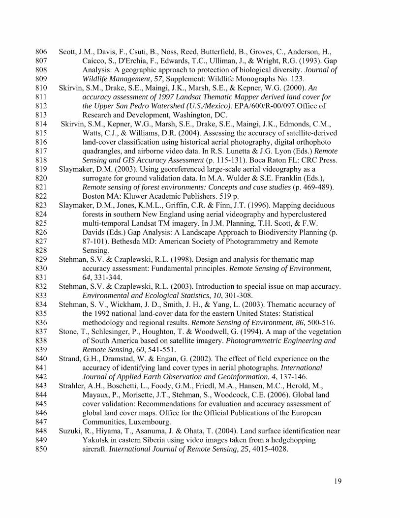
Table 1. Proportional allocation of first phase samples by EOSD stratum. Half of the samples were 875 allocated proportional to the area of each stratum, while the other half of the samples were allocated 876 to improve estimates for rare classes (see Czaplewski, 2003). 877

878

EOSD class Proportion of sampled

population mapped as xSample size

of x

water 0.0461 25 snow/ice 0.0217 19

rock/rubble 0.0000 14 exposed land 0.0324 22

shrub 0.0420 24 wetland treed 0.0074 16 wetland shrub 0.0016 14 wetland herb 0.0013 14

herb 0.0792 34 coniferous dense 0.0705 32 coniferous open 0.5391 149

coniferous sparse 0.1015 39 broadleaf dense 0.0185 19 broadleaf open 0.0377 23

broadleaf sparse 0.0007 14 mixed wood dense 0.0000 14 mixed wood open 0.0000 14

mixed wood sparse 0.0002 14

TOTAL 1.0000 500

879

880

22

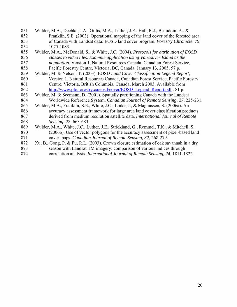
Table 2. Summary of results for all agreement scenarios with accuracy estimates followed by 90% 881 confidence intervals. 882

883

LEVEL 5 LEVEL 4

Agreement Scenario

Overall Accuracy

User's Accuracy

(for coniferous; variable density)

Overall Accuracy

User's Accuracy

(for coniferous)

EOSD and video primary

53% (49% - 57%)

coniferous dense 9%

(0.68% - 17%) coniferous open

72% (66% - 78%)

coniferous sparse 24%

(13% - 35%)

71% (68% - 74%)

coniferous 84%

(80% - 88%)

EOSD and video primary or secondary

61% (57% - 65%)

coniferous dense 23%

(11% - 35%) coniferous open

76% (70% - 82%)

coniferous sparse 33%

(21% - 45%)

73% (70% - 76%)

coniferous 85%

(81% – 89%)

EOSD 3x3 mode and

video primary or secondary

67% (64% - 70%)

coniferous dense 15%

(5% - 25%) coniferous open

82% (77% - 87%)

coniferous sparse 38%

(25% - 51%)

77% (74% - 80%)

coniferous 86%

(82% - 90%)

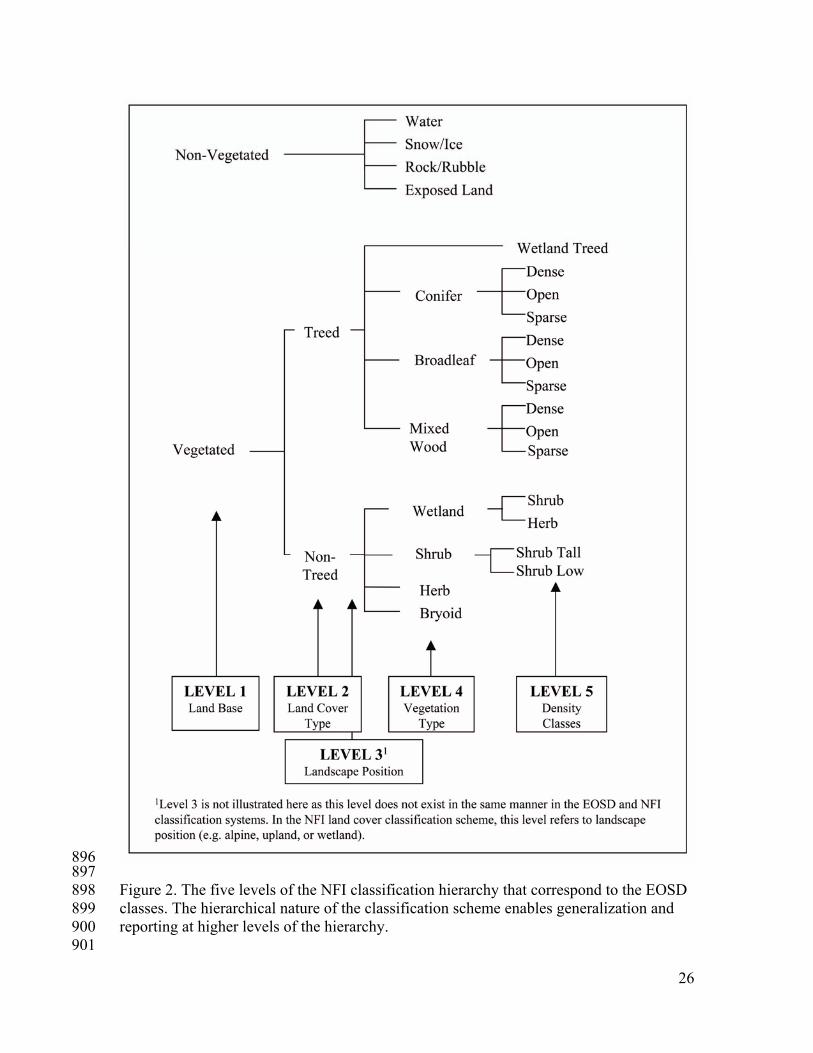
EOSD and forest

inventory

41% (37% - 45%)

coniferous dense 18%

(7% - 29%) coniferous open

55% (48% - 62%)

coniferous sparse 0%

(0% - 2.27%)

68% (66% - 71%)

coniferous 74%

(69% - 79%)

884

885

23

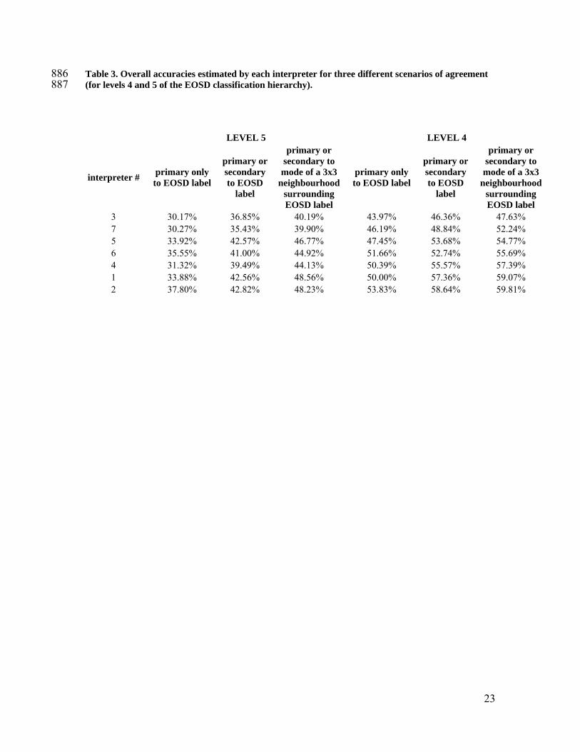
Table 3. Overall accuracies estimated by each interpreter for three different scenarios of agreement 886 (for levels 4 and 5 of the EOSD classification hierarchy). 887

LEVEL 5 LEVEL 4

interpreter # primary only to EOSD label

primary or secondary to EOSD

label

primary or secondary to

mode of a 3x3 neighbourhood

surrounding EOSD label

primary only to EOSD label

primary or secondary to EOSD

label

primary or secondary to mode of a 3x3

neighbourhood surrounding EOSD label

3 30.17% 36.85% 40.19% 43.97% 46.36% 47.63% 7 30.27% 35.43% 39.90% 46.19% 48.84% 52.24% 5 33.92% 42.57% 46.77% 47.45% 53.68% 54.77% 6 35.55% 41.00% 44.92% 51.66% 52.74% 55.69% 4 31.32% 39.49% 44.13% 50.39% 55.57% 57.39% 1 33.88% 42.56% 48.56% 50.00% 57.36% 59.07% 2 37.80% 42.82% 48.23% 53.83% 58.64% 59.81%

24

Table 4. Summary of overall interpreter agreement. 888

MINIMUM

% MAXIMUM

% MEAN

%

Level 5 51 71 60 Interpreter vs. interpreter (primary label only) Level 4 61 82 70

Level 5 67 90 77 Interpreter vs. interpreter (primary or secondary label) Level 4 70 92 81

Level 5 30 37 33 Interpreter vs. EOSD (primary label only) Level 4 44 54 49

Level 5 40 49 45 Interpreter vs. EOSD (primary or secondary label compared to the mode of a 3x3 neighbourhood around EOSD target pixel) Level 4 48 60 55

889 890

25

891

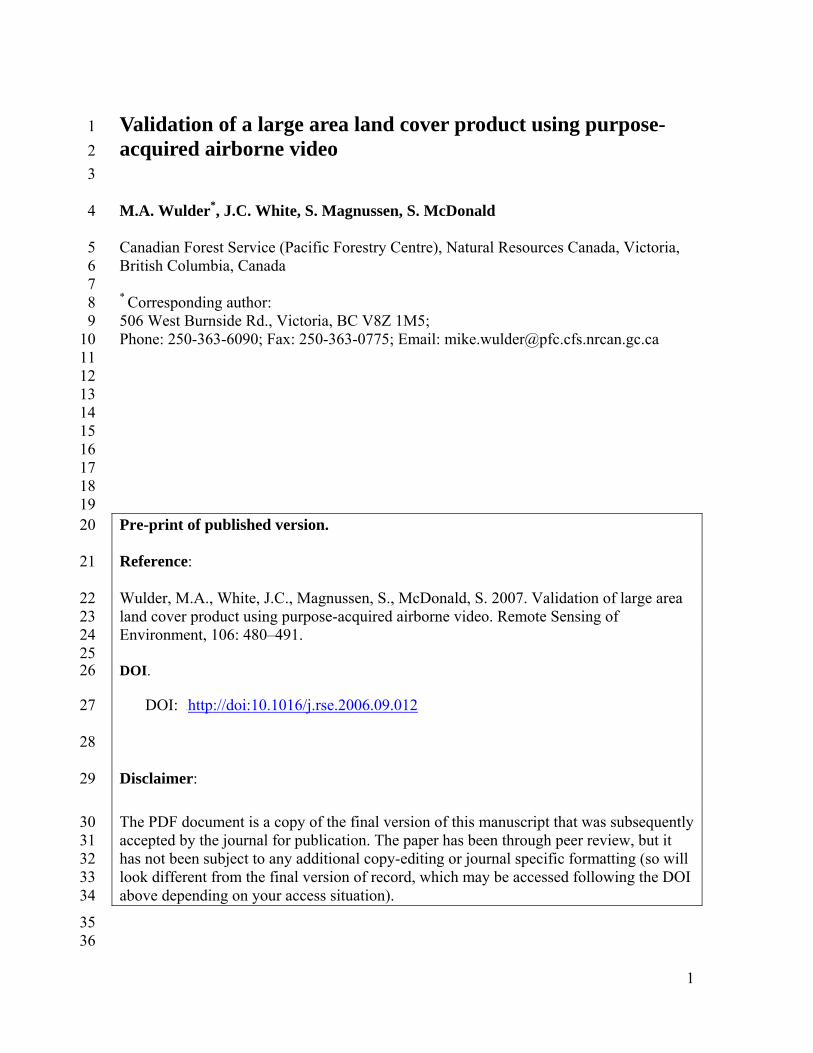
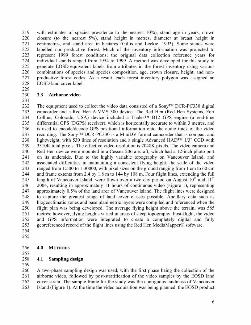
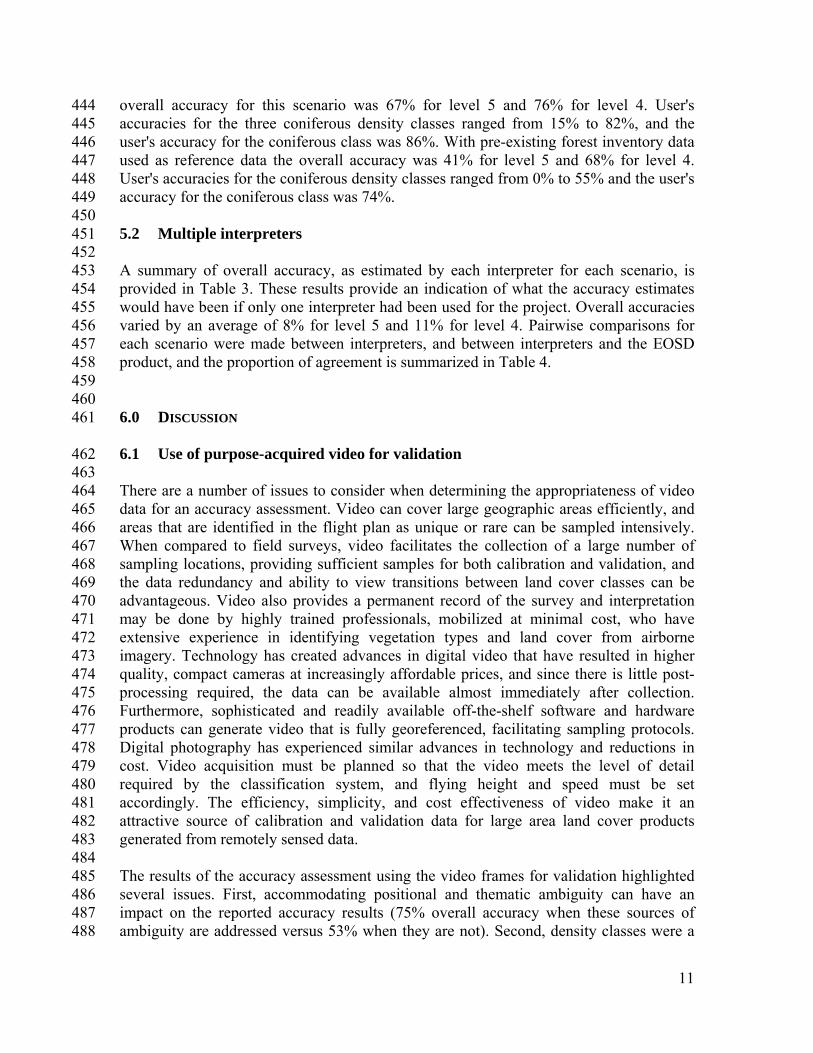
892 893 Figure 1. Vancouver Island, British Columbia is located on Canada's western coast. 894 Actual flight lines used for video collection are superimposed. 895

26

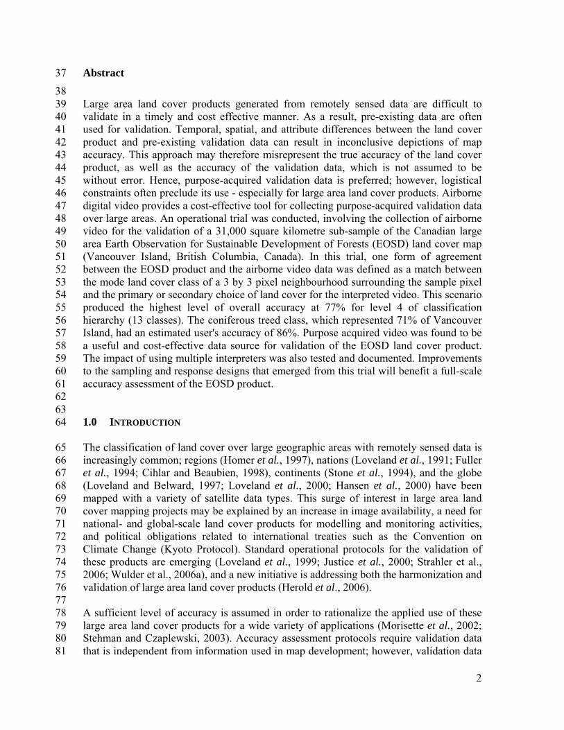
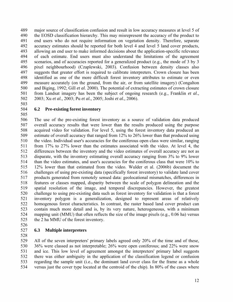
896 897 Figure 2. The five levels of the NFI classification hierarchy that correspond to the EOSD 898 classes. The hierarchical nature of the classification scheme enables generalization and 899 reporting at higher levels of the hierarchy. 900 901

27

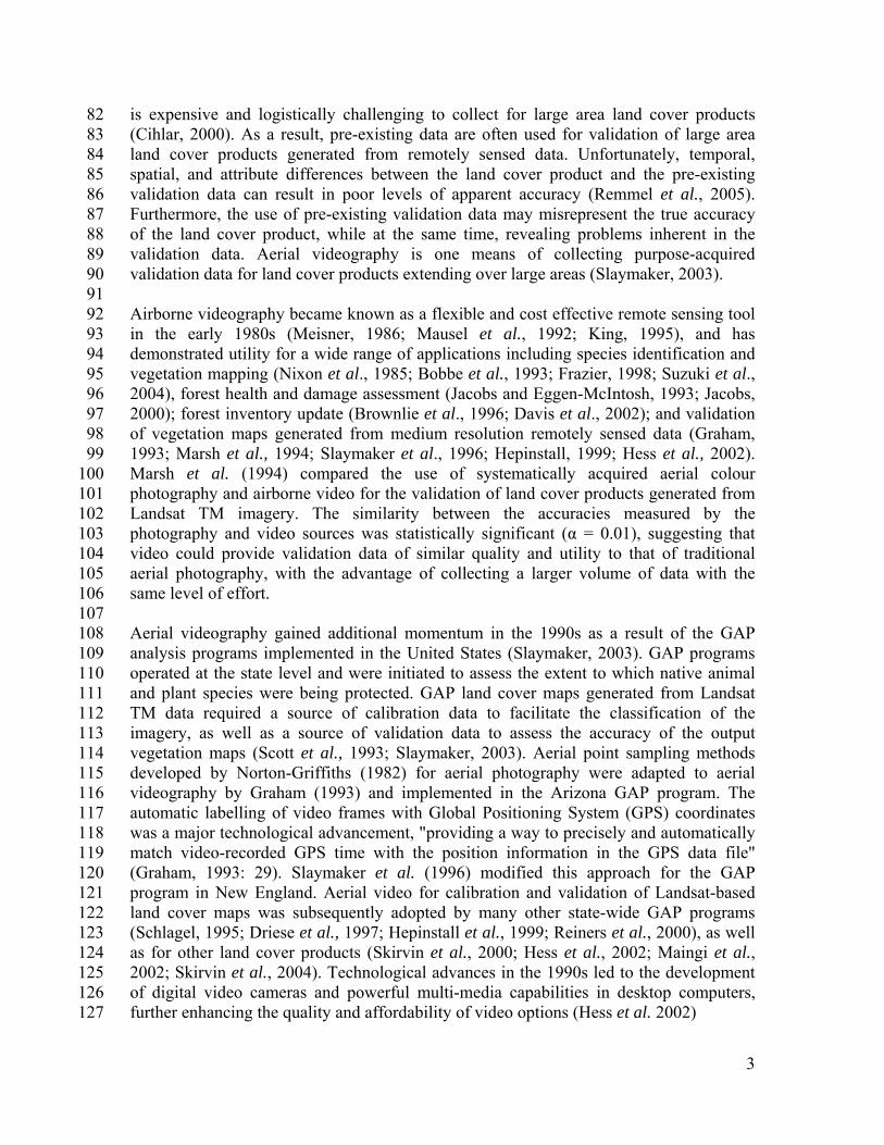
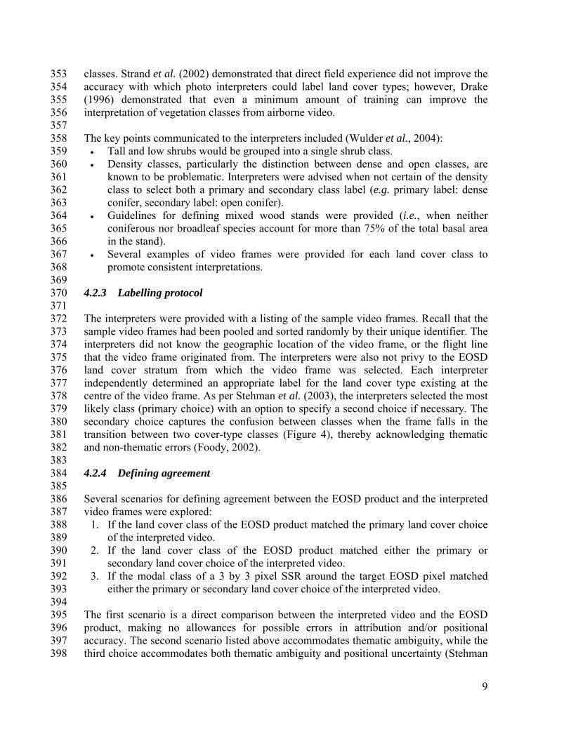
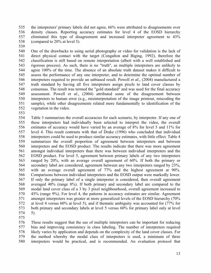
902 903 Figure 3. The planned flight lines for video acquisition draped over biogeoclimatic 904 zones/subzones and a digital elevation model. Actual flight lines are shown in Figure 1. 905 906

28

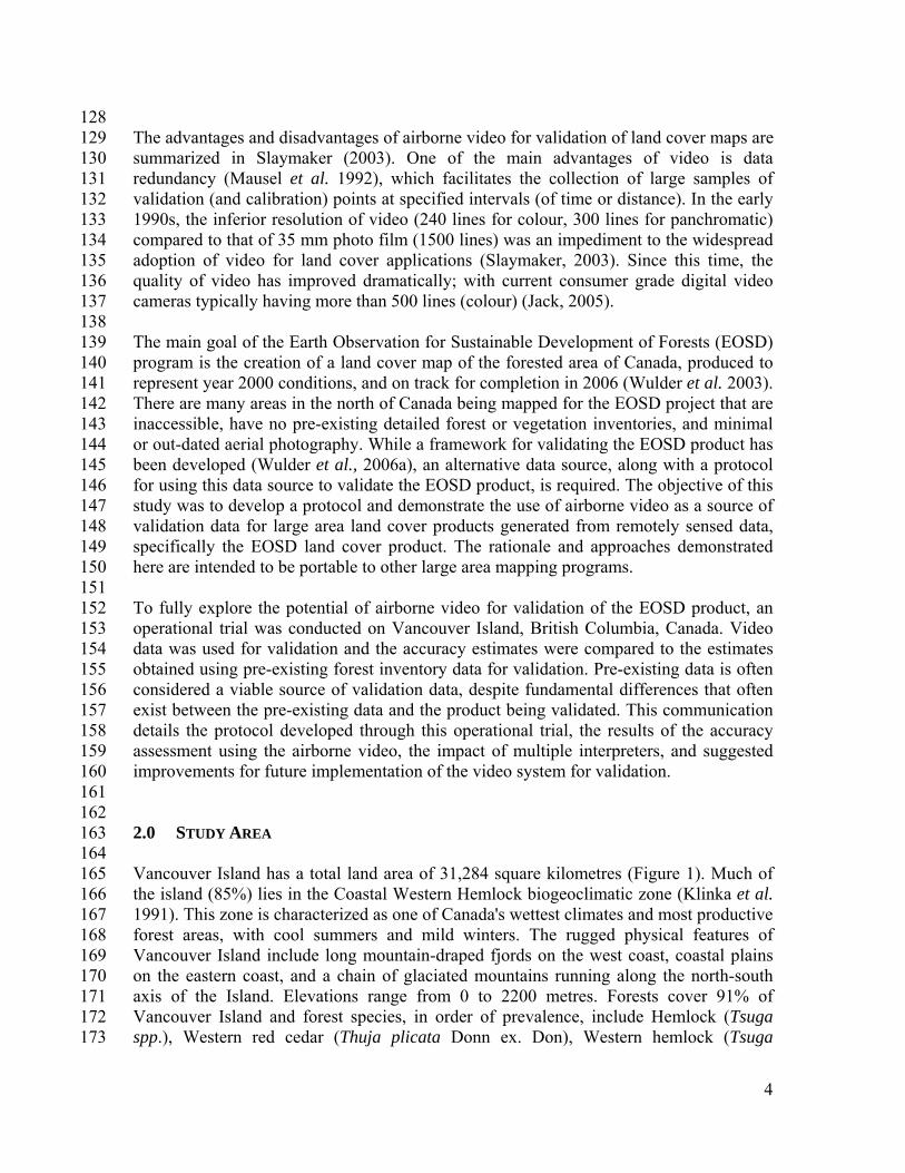
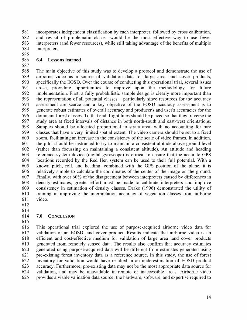
907 908 Figure 4. Examples of the need for using primary and secondary labels. 909 910