validation of ground biophysical products using imaging

Centre for Geo-Information Thesis Report GIRS-2005-14

VALIDATION OF GROUND BIOPHYSICAL PRODUCTS USING IMAGING SPECTROSCOPY IN A SOFTWOOD

FOREST

Taye Gidyelew Mengesha LAI

May

200

5

Validation of Ground Biophysical Products Using Imaging Spectroscopy in a Softwood Forest

Taye Gidyelew Mengesha

Registration number 75 09 05 557 090

Supervisors:

Prof. Dr. sc. nat. Michael E. Schaepman

Dr. ir. Sytze de Bruin

A thesis submitted in partial fulfillment of the degree of Master of Science at Wageningen University and Research Centre, The Netherlands.

May 2005 Wageningen, The Netherlands

Thesis code number: GRS-80337 Wageningen University and Research Centre Laboratory of Geo-Information Science and Remote Sensing Thesis Report: GIRS-2005-14

Acknowledgements This thesis is a result of a contribution from different organizations and individuals. First of all, I am deeply indebted to my supervisors for their valuable comments, critical contribution to this thesis and for being free to be consulted and share my research idea and progress. Thanks to Prof. Michael Schaepman for his continuous encouragement and answering my questions related to biophysical parameters derived from imaging spectrometer data. Thanks to Dr. ir. Sytze de Bruin for his help and contribution in geostatistical interpolation part of this study. Belgian Space Office (BELSPO) deserves many thanks for the STEREO programmme support and initiative for the HyMap data acquisition in the Millingerwaard. Many thanks for Joost Vandenabeele and VITO for their support. I also owe my gratitude to the Nuffic fellowship (NFP) for the financial support to pursue this study. I am grateful to my study advisor Willy ten Haaf for his advice and arrangement of conditions during my study. I am highly grateful to Dr. Fredric Baret and Marie Weiss for their consistent help concerning CAN_EYE questions. The cooperation of the staff from Alterra and CGI makes my fieldwork so successful and easy. I would particularly like to thank Jan Clement, Raul Milla Zurita, Jan Hein Loedeman, Lammert Kooistra and my friends; Teshome Eshete and Angela kross for their cooperation and help in a difficult and jungle softwood forest. I would like to thank all my friends of MGI here in the Netherlands and particularly, special thank goes to Worku, Jie, Tine, Lucie, Elisa and Babs for making our time at Alterra so enjoyable. Thanks Ates for your advice and support through prayer. Many people (they know where and who they are) have contributed to my study. Due to limited page to include their names exhaustively, I extend big thank to all of them.

I would also like to take this opportunity to express my heart felt thank to my families for their contribution in my study from early childhood. My heart felt thank goes to the family of Van de Put (Bart and Willy) for their special and kind hospitality at their home and for showing me historical places in the Netherlands. The encouragements and the nice relationship with their children and grand children in the Netherlands will never be forgotten. I owe a very special thanks to you all, the families of Van de Put. Last but not least my special thank goes to my beloved wife, Martha Yohannes for her splendid love, patient, understanding, support and encouragement to pursue my interest. Glory be to God for ever and ever!

I

Abstract The demand for timely and accurate information on the status and functioning of forest biomes for monitoring land biosphere and variety of purposes is increasing. Leaf Area Index (LAI) is thus the key biophysical variable influencing land surface processes such as photosynthesis, transpiration and energy balance and is required for various ecological models. Recent advances in validation of vegetation products have led to new ground based methods to assess the accuracy for small and large spatial footprint sensors. We conducted a study to generate a continuous, validated, spatially explicit map of vegetation variables (e.g., LAI, Fraction of Absolved Photosynthetically Active Radiation (fAPAR), Fractional Cover (fCover)) in a softwood forest derived from HyMap data. These products were also compared with a geostatistically-interpolated map of ground measurements following the VALERI sampling scheme in a river floodplain of the Netherlands. Millingerward is located near the German-Dutch border with a natural reserve area composed of softwood forest species namely Populus nigra L., Salix alba L., and Salix fraglis L. and dense understory namely Urtica dioica L. Calamagrostis epigejos (L.) Rubus caesius L. The ground measurement was done using hemispherical photography to assess the forest biophysical products through measuring gap fraction and gap size distribution in the forests for calibration of the airborne measurements taken over the Millingerwaard during summer 2004. A total of 156 points (e.g., 13 plots, each with 12 sub-sampling points) have been measured and processed using a neural network based approach for validation and calibration purposes of LAI. The WDVI was used to derive LAI from the imaging spectrometer data and calibrated based on the ground measurements. The ground measured LAI and the HyMap derived LAI using WDVI has shown a good correlation (r2 = 0.82). The results from the ground measurements coupled with the HyMap derived fCover was used for the geo-statistical interpolation approach. The LAI values are interpolated over the whole area of the softwood forest by simple kriging method with varying local mean and spatial explicit map, which can be used for the validation and calibration of larger footprint sensors was produced. The sensitivity of the different vegetation indices was also tested using various LAI retrieval algorithms such as; RSR, FVC, and NDVI. Even though, the different vegetation indices have resulted in different values, the LAI value derived using WDVI and RSR showed good correlation (r2=0.88). Generally the selected approaches enabled to produce validated continuous fields of biophysical products with good accuracy and well suited to derive LAI on a forest stand scale. Keywords: Imaging Spectroscopy, Leaf Area Index, hemispherical photography, geostatistical interpolation, validation, forest biophysical products

II

Table of Contents ACKNOWLEDGEMENTS .......................................................................................................................... I ABSTRACT ................................................................................................................................................. II TABLE OF CONTENTS...........................................................................................................................III LIST OF FIGURES......................................................................................................................................V LIST OF TABLES.................................................................................................................................... VII ABBREVIATIONS .................................................................................................................................VIII 1. INTRODUCTION .................................................................................................................................... 1

1.1. BACKGROUND ..................................................................................................................................... 1 1.2. PROBLEM DEFINITION.......................................................................................................................... 2 1.3. RESEARCH OBJECTIVES........................................................................................................................ 3 1.4. STRUCTURE OF THE REPORT ................................................................................................................ 3

2. LITERATURE REVIEW ........................................................................................................................ 4 2.1. DEFINITION OF TERMS.......................................................................................................................... 4

2.1 1. LAI Definition According to Different Literatures...................................................................... 4 2.1 2. Canopy Structure ........................................................................................................................ 4 2.1.3. Contact Frequency and Gap Fraction ........................................................................................ 5 2.1.4 Leaf Area Density (LAD) and (LIDF).......................................................................................... 6

2.2. INDIRECT LAI MEASUREMENT ............................................................................................................ 6 2.3. LAI ESTIMATION BASED ON GAP FRACTION MEASUREMENT ............................................................. 7 2.4. LAI ASSESSMENT TECHNIQUES AND INSTRUMENTS............................................................................ 9

2.4.1 LAI-2000 Plant Canopy Analyzer (PCA) ..................................................................................... 9 2. 4.2. Tracing Radiation and Architecture Canopies (TRAC) ........................................................... 10 2.4.3. Hemispherical Canopy Photography........................................................................................ 11

2.5. IMAGING DEVICES AND IMAGE PROCESSING ..................................................................................... 11 2. 6. VEGETATION INDICES FOR LAI ESTIMATION .................................................................................... 13 2.7. LINEAR SPECTRAL UNMIXING TO DERIVE FCOVER. .......................................................................... 14 2.8. GEOSTATISTICAL APPROACH............................................................................................................. 14

2.8. 1.Geo-statistical Interpolation Method........................................................................................ 14 3. METHODOLOGY................................................................................................................................. 16

3.1. STUDY AREA ..................................................................................................................................... 16 3.2. AIRBORNE AND FIELD DATA ............................................................................................................. 17 3.3. LAI GROUND SAMPLING ................................................................................................................... 18 3.4. HEMISPHERICAL PHOTOGRAPH ACQUISITION AND PROCESSING........................................................ 19

3.4.1. Basic Principles of Hemispherical Photograph Processing ..................................................... 20 3.4.2. Algorithms implemented to derive LAI by CAN_EYE ............................................................... 20

3.5. SPECTRORADIOMETRIC FIELD MEASUREMENTS ................................................................................ 21 3.6. DESCRIPTION OF HYMAP DATA QUALITY.......................................................................................... 21

3.6.1. Mean and Standard Deviation .................................................................................................. 25 3.6.2. Saturation.................................................................................................................................. 26 3.6.3. Correlation Matrices................................................................................................................. 27 3.6.4.Image Based Signal to Noise Ratio (SNR) ................................................................................. 27

3.7. BIOPHYSICAL PARAMETER RETRIEVAL FROM HYMAP IMAGE........................................................... 28 3.7.1. Weighted Difference Vegetation Index (WDVI) ........................................................................ 29 3.7.2 Green Red Vegetation Index (GRVI).......................................................................................... 30

3.8. SENSITIVITY TEST OF LAI RETRIEVAL ALGORITHMS ........................................................................ 30 3.9. VEGETATION FRACTIONAL COVER (FCOVER).................................................................................... 31 3.10. FRACTION OF ABSORBED PHOTOSYNTHETICALLY ACTIVE RADIATION (FAPAR) ........................... 32

III

3.10.1. fAPAR from Hemispherical Photographs ............................................................................... 32 3.10.2. fAPAR from HyMap data ........................................................................................................ 33

3.11. GEO-STATISTICAL INTERPOLATION.................................................................................................. 33 4. RESULTS AND DISCUSSION............................................................................................................. 35

4.1. BIOPHYSICAL PRODUCTS FROM HEMISPHERICAL PHOTOGRAPHY ...................................................... 35 4.1.1. LAI ............................................................................................................................................ 35 4.1.2. Gap Fraction............................................................................................................................. 36 4.1.3. Fractional Vegetation Cover (fCover) ...................................................................................... 39 4.1.4. Fraction of Absorbed Photosynyhetically Active Radiation (fAPAR) ....................................... 39

4.2. BIOPHYSICAL PRODUCTS DERIVED FROM HYMAP ............................................................................ 39 4.2.1. LAI ............................................................................................................................................ 39 4.2.2. Fraction of Vegetation Cover (fCover) ..................................................................................... 44

4.2.1.1. Fractional Vegetation Cover Derived Using GRVI............................................................................ 44 4.2.1.2 Fractional Vegetation Cover Using Linear Spectral Unmixing Approach .......................................... 44

4.2.3. Fraction of Absorbed Phothosynthetically Active Radiation (fAPAR)...................................... 45 4.3. GEOSTATISTICALLY INTERPOLATED LAI........................................................................................... 46 4.4. COMPARISON OF LAI RESULTS FROM HEMISPHERICAL CAMERA AND HYMAP ................................. 48 4.5. SPECTRAL LIBRARY BUILDING .......................................................................................................... 50

5. CONCLUSIONS AND RECOMMENDATIONS................................................................................ 52 5.1. CONCLUSIONS.................................................................................................................................... 52 5.2. RECOMMENDATIONS ......................................................................................................................... 53

6. REFERENCES ....................................................................................................................................... 54 7. APPENDIX ............................................................................................................................................. 61

IV

List of Figures FIGURE 1. LOCATION OF THE STUDY AREA,TOP MILLINGERWARD AT DUTCH -GERMAN BORDER, MIDDLE-

TOPOGRAPHIC MAP OF MILLINGERWARD AREA AND BOTTOM- SOFTWOOD FOREST IMAGE FROM HYMAP SENSOR. ............................................................................................................................................... 16

FIGURE 2. CONCEPTUAL MODEL FOR DERIVING SPATIALLY DISTRIBUTED LAI MAP FROM AIRBORNE AND GROUND MEASUREMENTS AND PROCESSING STEPS. ............................................................................. 17

FIGURE 3. A).DISTRIBUTION OF SAMPLE PLOTS IN THE SOFTWOOD FOREST ON TOP OF HYMAP IMAGE, AND (B).THE FIELD LAYOUT FOR DIGITAL HEMISPHERICAL PHOTOGRAPHY ACCORDING TO VALERI PROTOCOL............................................................................................................................................ 18

FIGURE 4. HEMISPHERICAL PHOTOGRAPHS. LEFT, DOWNWARD HEMISPHERICAL PHOTOGRAPH RIGHT, UPWARD HEMISPHERICAL PHOTOGRAPHS TAKEN FROM ONE POINT IN THE SAMPLE PLOTS................... 19

FIGURE 5: HYMAP SPECTRAL BAND POSITIONS VS. SPECTRAL RESOLUTION (FWHM) OF ALL 126 SPECTRAL BANDS.................................................................................................................................................. 23

FIGURE 6. HYMAP VIS DETECTOR BAND POSITIONS AND FWHM. ............................................................... 24 FIGURE 7. HYMAP NIR DETECTOR BAND POSITIONS AND FWHM................................................................ 24 FIGURE 8. HYMAP SWIR1 DETECTOR BAND POSITIONS AND FWHM........................................................... 25 FIGURE 9. HYMAP SWIR2 DETECTOR BAND POSITIONS AND FWHM........................................................... 25 FIGURE 10. HYMAP MINIMUM, MAXIMUM, MEAN AND STANDARD DEVIATION, ............................................ 26 FIGURE 11. HYMAP VERY BRIGHT AND VERY DARK TARGET ........................................................................ 26 FIGURE 12. FLOW CHART OF METHODOLOGY FOR INTERPOLATION OF LAI IN THE SOFTWOOD FORESTS IN

MILLINGERWARD USING SIMPLE KRIKING METHOD. ............................................................................ 33 FIGURE 13. INVERSED EXPONENTIAL RELATION SHIP OF MEASURED LAIEFF AND GAP FRACTION OBTAINED

FROM HEMISPHERICAL PHOTOGRAPHS OVER THE 13 VALERI SAMPLE PLOTS IN THE SOFTWOOD FORESTS AT THE MILLINGERWAARD.................................................................................................... 36

FIGURE 14. GAP SIZE DISTRIBUTION FOR RINGS BETWEEN 55 -60O FROM DOWNWARD HEMISPHERICAL PHOTOGRAPHS OF SOFTWOOD FOREST AT MILLINGERWAARD INVALERI SAMPLE PLOT 2.................. 37

FIGURE 15 MEASURED GAP FRACTION VS LUT GAP FRACTION AND AVERAGE LAI, ALA, FCOVER FROM DOWNWARD HEMISPHERICAL PHOTOGRAPHS OF VALERI SAMPLE PLOT 2.......................................... 37

FIGURE 16 GAP FRACTION IMAGE AFTER CAN_EYE PROCESSING FROM DOWNWARD HEMISPHERICAL PHOTOGRAPHS OF VALERI SAMPLE PLOT 2. ....................................................................................... 38

FIGURE 17 CLUMPING FACTOR AT DIFFERENT VIEW ZENITH ANGLE FROM DOWNWARD HEMISPHERICAL PHOTOGRAPHS OF VALERI SAMPLE PLOT 2. ....................................................................................... 38

FIGURE 18. SPATIALLY DISTRIBUTED MAP OF LAI BASED ON WDVI AT MILLINGERWAARD. ....................... 41 FIGURE 19. SPATIALLY DISTRIBUTED MAP OF LAI BASED ON RSR IN MILLINGERWAARD............................ 41 FIGURE 20. SPATIALLY DISTRIBUTED MAP OF LAI BASED ON FVC IN MILLINGERWAARD.......................... 42 FIGURE 21.SPATIALLY DISTRIBUTED MAP OF LAI BASED ON NDVI AT MILLINGERWAARD ......................... 42 FIGURE 22. GRAPHICAL PLOT OF THE RESULTS OF APPLICATION OF DIFFERENT ALGORITHMS TO HYMAP

IMAGE AND CAN_EYE DERIVED LAI VALUES AT A PLOT LEVEL IN THE SOFTWOOD FORESTS AT MILLINGERWAARD .............................................................................................................................. 43

FIGURE 23. FCOVER MAP FOR THE SOFTWOOD FOREST AREA IN THE MILLINGERWAARD (PIXEL SIZE AGGREGATED TO 20X20 METER).......................................................................................................... 45

FIGURE 24. SEMIVARIGORAM OF RESIDUAL LAI PLOTS FOR THE 13 VALERI SAMPLE PLOTS OF SOFTWOOD FOREST. ............................................................................................................................................... 46

FIGURE 25 LAI AND FCOVER RELATIONSHIP DERIVED FROM GROUND MEASUREMENTS USING CAN_EYE FOR ALL 13 SAMPLING PLOTS IN THE SOFTWOOD FORESTS AT THE MILLINGERWAARD SITE........................ 47

FIGURE 26. LAI VALUES PER VALERI SAMPLE PLOT VS LAI VALUES FROM KRIGING AND CAN_EYE IN THE SOFTWOOD FOREST AT MILLINGERWAARD. ......................................................................................... 47

FIGURE 27. SPATIALLY DISTRIBUTED MAP OF LAI INTERPOLATED BY SIMPLE KRIGING IN THE SOFT WOOD FOREST AREAS AT MILLINGERWAARD (PIXEL SIZE OF GRID 20 M X 20 M). ........................................... 48

FIGURE 28. LAI DERIVED FROM HYMAP BASED ON WDVI IN THE SOFTWOOD FOREST AT MILLINGERWAARD............................................................................................................................................................. 48

FIGURE 29. COMPARISON OF MEASURED LAI FROM GROUND MEASUREMENT AND HYMAP FOR EACH PLOTS............................................................................................................................................................ 49

V

FIGURE 30 CORRELATION OF EFFECTIVE LAI FROM HYMAP AND HEMISPHERICAL PHOTOGRAPHS FOR 13 VALERI SAMPLE PLOTS IN THE SOFT WOOD FOREST IN THE MILLINGERWAARD. ................................ 49

FIGURE 31. THE PERCENTAGE DIFFERENCE MAP OF LAI FROM WDVI AND SPATIALLY INTERPOLATED APPROACH. .......................................................................................................................................... 50

FIGURE 32. AVERAGE REFLECTANCE FROM SPECTRAL LIBRARY FOR THE MAJOR TREE SPECIES IN SOFTWOOD FORESTS AT LEAF LEVEL MEASURED BY ASD FIELD SPECTROMETER .A) AN AVERAGE OF MAXIMUM, MINIMUM AND AVERAGE REFLECTANCE OF POPULUS NIGR’S A LEAVES B) AN AVERAGE OF MAXIMUM, MINIMUM AND AVERAGE REFLECTANCE OF SALIX ALBA’S LEAVES C.) AN AVERAGE OF MAXIMUM, MINIMUM AND AVERAGE REFLECTANCE OF SALIX FRAGILIS’S LEAVES................................................... 51

VI

List of Tables TABLE 1. HYMAP PARAMETERS AND UNITS FOR THE HYECO’04 CAMPAIGN. ............................................... 22 TABLE 2. HYMAP PARAMETERS FOR HYECO’04: COVERING THE SOFTWOOD AREA. .................................... 23 TABLE 3. SUMMARY OF ALL GROUND MEASURED BIOPHYSICAL PRODUCTS IN THE 13 VALERI SAMPLE PLOTS

IN SOFTWOOD FORESTS OF THE MILLINGERWAARD. ............................................................................ 35 TABLE 4. SUMMARY OF BIOPHYSICAL PRODUCTS DERIVED FROM HYMAP IMAGE PER EACH SAMPLE PLOTS

FOR THE SOFTWOOD FORESTS AT MILLINGERWAARD .......................................................................... 40 TABLE 5. STATISTICS OF GRVI RESULTS BEFORE AND AFTER SCALING THE VALUES TO 0 AND 1. ................. 44 TABLE 6. STATISTICS OF LINEAR SPECTRAL UNMIXING RESULTS BEFORE AND AFTER SCALING TO 0 AND 1.. 45

VII

VIII

Abbreviations ALA Average Leaf Inclination Angle [0-90o]

APAR Absorbed Photosynthetically Active Radiation [W m-2 nm -1]

ASCII American Standard Code for Information Interchange ASD Analytical Spectral Devices

BELMINP Bench Mark Land Multisite Intercomparision of Products

CEOS-LPV Committee Earth Observation Study- Land Product Validation

DN Digital Number

ENVI ENvironment of VIsualization

FAI Foliage Area Index [m2 m-2]

fAPAR Fraction of Absorbed Photosynthetically Active Radiation [W m-2 nm -1]

fCover Fractional cover

FOV Field of View

FVC Fraction Vegetation Cover

GRVI Green Red Vegetation Index

HyMap Hyperspectral Mapper

IDL Interface Definition Language

IFOV Instantaneous Field of View

LAD Leaf Area Density [m2 m-3]

LAI Leaf Area Index [m2 m-2]

LIDF Leaf Inclination Distribution Function

LUT Look Up Table

MSAVI Modified Soil Adjusted Vegetation Index

NDVI Normalized Difference Vegetation Index

nm Nanometer

NPP Net Primary Production [ton of C/ha]

PAI Plant Area Index [m2 m-2]

PAR Photosynthetically Active Radiation [W m-2 nm -1]

PCA Plant Canopy Analyzer

RSR Reduced Simple Ratio

RTM Radiative Transfer Model

SR Simple Ratio

SWIR Short Wave Infra Red

TRAC Tracing Radiation and Architecture Canopies

UTM Universal Transverse Mercator

VAI Vegetation Area Index [m2 m-2]

VALERI Validation of Land European Remotesensing Instruments

WDVI Weighted Difference Vegetation Index

WGS84 World Grid System 84

1. Introduction

1. Introduction 1.1. Background Nowadays the demand for timely and accurate information on the status and functioning of forest biomes, for a variety of purposes, is increasing. While traditionally forest information was gathered using in-situ methods, the role of remote sensing is becoming more and more central because of the need to the spatial and temporal variability of the key forest processes. Forests provide essential economic and ecological services and their essential role in the planetary system is being increasingly recognized. However, as of today, it is still not known for sure if forests will become a sink or a source of CO2 in the long run (Cox et al., 2000). Several studies have shown that hyperspectral remote sensing techniques can be applied for quantitative characterization of biophysical and biochemical variables to fulfill this information gap. These studies have shown that biophysical and biochemical variables can be measured with quantifiable uncertainty (Hu et al., 2000; Rast et al., 2004; Kotz et al., 2004; Schaepman et al., 2004 ; Schlerf et al., 2005) . Leaf area index (LAI) is essential for numerous studies of atmosphere- vegetation interaction, as it is very often a critical parameter in process-based models of vegetation canopy response to global environmental change (Jonckheere et al., 2004). It determines the size of the plant-atmosphere interface and thus plays a key role in the exchange of energy and mass between the canopy and the atmosphere. Moreover, under certain assumptions, knowledge of canopy structure variables Leaf area Density (LAD) and Leaf Inclination Distribution Function (LIDF) allows the evaluation of the fraction of Absorbed Phothesynthetically Active Radiation (fAPAR), which is required to model the canopy’s phothesynthetic activity in a straightforward way (Monteith, 1977). LAI is therefore mentioned as a key variable frequently used as input for crop growth models (Broge and Leblanc, 2001) . Consequently, recent in-situ and above canopy remote sensing techniques have focused on the measurement and use of LAI as a structural variables since the variables that describe vegetation canopy structure and its energy absorption capacity are required by many of the EOS Interdisciplinary Projects (Myneni et al., 1997). LAI can be estimated for, indirect light measurement within the canopy by an instrument looking at zenith or towards the sun. Several techniques provide angular information about the amount and distribution of openings in the canopy, often called gap fraction (Normal and Campbell, 1989). Hence assessment of relevant forest variables can be adequately performed by the use of Radiative Transfer Models (RTM) since these models take into account physical processes describing the interaction of radiation with the diverse canopy components at foliage and canopy levels (Myneni and Ross, 1991). Radiative transfer models have already been successfully employed with homogeneous canopies to derive quantitative information on canopy structure and foliage biochemistry (Faurtyot and Baret, 1997; Weiss and Baret, 1999; Weiss et al., 1999; and Jacquemoud et al., 2000). Some models

1

1. Introduction

have been compared in performance and quality extensively (Pinty et al., 2001, 2004) and are toady used in many remote sensing derived products (e.g., MODIS MOD15). Usually this approach considers the spectral reflectance of a plant canopy which is known to be primarily a function of the foliage optical properties, the canopy structure, the understory and soil background reflectance, the illumination conditions, and also the viewing geometry (Goel and Grier, 1988; Chen et al., 2000). Recently hemispherical photography has been increasingly used to characterize the structure of canopies and measure the gap fraction directional variation to retrieve variables such as the LAI, fAPAR and clumping factor due to its potential to overcome a number of problems (e.g., greenness confusion and gap size distribution for computing foliage clumpiness) (Jonckheere et al., 2004; Weiss et al., 2004). These approaches are now used to validate LAI on WGCV (global) scales (Privette et al., 2001). We will use regional LAI measurements made with a hemispherical camera and subsequent analysis for calibration and validation purposes of airborne imaging spectrometer data and the retrieved biophysical products from this image will be compared to a geostatistically interpolated map of LAI over a softwood forest in a river floodplain in the Netherlands. 1.2. Problem Definition Direct methods of LAI estimation are the most accurate, but they have the disadvantage of being extremely time-consuming and as a consequence making large-scale implementation only marginally feasible. Accuracy problems may in this case result from the definition of LAI, the up-scaling method, or from the error accumulation due to frequently repeated measurements. As it has been explained by (Chason et al., 1991) because of its time-consuming and labor-intensive character and operational constraints, it can be said that direct LAI determination is not really compatible with long-term monitoring of spatial and temporal dynamics of leaf area development. However, the need for validation of indirect methods remains, so the direct techniques can be considered important as calibration methods. Several studies have been carried out on the use of different vegetation indices for LAI estimation (Qi et al., 1994; Brown et al., 2000; and Haundance et al., 2004). A major problem in the use of the different vegetation indices arises from the fact that canopy reflectance in the visible and near infrared is strongly dependent on both the structural (i.e., LAI) and biochemical properties (e.g., chlorophyll) of the canopy. Moreover LAI and chlorophyll content have a similar effect on canopy reflectance particularly in the spectral region ranging from the green (500 nm) to the red edge (750 nm), (Goel and Grier, 1988; Jacquemoud et al., 2000; Zarco-Tejada et al., 2001). Therefore this study focuses on the use of hemispherical camera for an improved estimation of the gap fraction, since hemispherical photograph is a convenient technique that offers the potential to account for foliage clumping and greenness confusion, which may very significantly affect the characterization of important vegetation types (Fernandes et al., 2002).

2

1. Introduction

1.3. Research objectives The research objectives of this study are therefore: 1. to generate a spatially explicit map of vegetation structure in a softwood forest, 2. to calibrate and validate the biophysical variable retrieval (LAI, fAPAR and

fCover) from imaging spectrometer data using ground measurements, and 3. to interpolate ground measurements using geostatistical approach supported by

products derived from Imaging Spectrometer data and ground measurements for validation of large footprint sensors.

The specific objectives are to:

− quantify spatially distributed structural characteristics of a softwood forest canopy using a hemispherical camera and neural network based analysis software to retrieve the gap fraction, LAI clumping factor, fAPAR, and fCover,

− test the sensitivity of a set of procedures to retrieve spatially distributed LAI from imaging spectrometer data,

− interpolate the ground measurements using kriging and scaling approaches for comparison of product quality, and

− build a spectral library of leaf optical properties of the softwood forest for spectral unmixing of species.

The Research questions related to the objectives are:

− How can we build a spatially distributed LAI map from hemispherical photographs for calibration of imaging spectrometer data at the stand scale?

− Can quality measures be derived to estimate the potential of LAI maps for ecological modeling based on the selected approach?

− Can these approaches further be supported using leaf optical properties measurements for spectral unmixing approaches?

1.4. Structure of the Report Chapter one of this report is an introduction about a general background and explanation about the definition of the topic and the use of biophysical products where specifically the LAI is included. The objectives of this study and research questions are also covered in this chapter. Chapter two deals with review of relevant literatures and discusses similar studies conducted in the field of biophysical vegetation products. The third chapter describes the methodologies followed in order to achieve the research objectives. The results of this study are also presented and discussed in chapter four and conclusion and recommendations are given in the fifth chapter. Lists of cited literatures and appendix are given at the end of the thesis.

3

2. Literature Review

2. Literature Review This chapter of this paper deals with relevant literatures and studies conducted in similar areas of interest. It also gives an insight about the theoretical background about this research topic by discussing related works. 2.1. Definition of terms The most commonly used terminologies in this study are defined in the following sub sections based on the referred literatures.

2.1 1. LAI Definition According to Different Literatures The definition of LAI was given by different authors and all the definition vary according to the interest of the individuals. Here are some of the definitions about LAI from the literature. LAI was first defined as the total one-sided area of photosynthetic tissue per unit ground surface area (Watson, 1947). For broad-leaved trees with flat leaves, this definition is applicable because both sides of a leaf have the same surface area. However, if foliage elements are not flat, but wrinkled, bent or rolled, the one-sided area is not clearly defined. Similar problems exist for coniferous trees, as needles may be cylindrical or hemi-cylindrical (Chen and Black 1992). Some authors therefore proposed a projected leaf area in order to take into account the irregular form of needles and leaves (Bolstad and Gower, 1990; Smith, 1991). However, in this case the choice of projection angle is decisive, and a vertical projection does not necessarily result in the highest values. Myneni et al. (1997) consequently defined LAI as the maximum projected leaf area per unit ground surface area. Within the context of the computation of the total radiation interception area of plant elements, and based on calculations of the mean projection coefficients of several convex and concave objects of different angular distributions. Lang (1991), and Chen and Black (1992) suggested that half the total interception area per unit ground surface area would be a more suitable definition of LAI for non-flat leaves than the projected leaf area. Their theoretical reasoning behind abandoning the projection concept was that the latter has neither physical nor biological significance, whereas the total intercepting area has a physical meaning (e.g., radiation interception) and the total area has a biological connotation (e.g., gas exchange). Still other definitions and interpretations of LAI have been proposed. These vary depending on the technique used to measure the LAI. Following current literature and also in this study, LAI is defined as one half the total leaf area per unit ground surface area (Chen et al., 1991; Chen and Black 1992; Fassnacht et al., 1994; and Stenberg et al., 1994). It is therefore important to note that the choice of the LAI definition can result in significant differences between calculated LAI values.

2.1 2. Canopy Structure The knowledge of temporal and spatial variability of vegetation canopy properties is recognized as a key element for understanding terrestrial biosphere process and can assist the parameterization of various physical and ecological models which include the vegetation as a dynamic component (e.g., Sellers and Schmid, 1993; Verstaete et al., 1994).

4


Canopy structure is characterized by the position orientation, size, and shape of the vegetative elements (Ross, 1981). The distribution of optical properties may also be considered as being part of the canopy structure. Canopy architecture changes with time scales varying from fraction of seconds and minutes (wind water stress, etc) to seasons (phenological evolution, environmental constraints) and years (ecosystem dynamics). An exhaustive and detailed description of a canopy structure is not easy due to its spatial heterogeneity and thus, large number of measurements required which is tedious and time consuming (Lang et.al., 1985). Therefore in many cases, the canopy structure is described with only a few variables, such as the Leaf Area Density (LAD) and the Leaf Inclination Distribution Function (LIDF) (Weiss et al., 2004).

2.1.3. Contact Frequency and Gap Fraction Contact frequency is the probability that a beam (or a photon) penetrating inside a canopy will come in to contact with a vegetative element (Chen and Black, 1991). Conversely, gap frequency is the probability that this beam will have no contact with the vegetative elements until it reaches a reference level (generally the ground). Then the term ‘gap fraction’ is often used and refers to the integrated value of the gap frequency over a given domain and thus, refers to the quantity that can be measured. Therefore, measuring gap fraction is equivalent to measuring the transmittance at ground level, at wavelengths for which the assumption of black vegetative elements is valid. (Weiss et al., 2004). It is then possible to consider the mono-directional gap fraction, which is the fraction of ground observed in a given viewing direction (or illuminated in a given incident direction). The bi-directional gap fraction is the fraction of soil (or area of a horizontal reference level) which is both illuminated in a given direction and observed in another (Qin and Goel, 1995). When both directions are collinear, the bi-directional gap fraction is equal to the mono-directional gap fraction. This corresponds to the well-known "hot-spot" feature observed in the backscattering direction when measuring canopy reflectance; in other words, no shadow except that of the sensor can be observed in this particular geometric condition (Gerstl and Simmer, 1986; Breon et al. 1997).

The contact frequency is a very appealing quantity to indirectly estimate LAI because no assumptions on leaf spatial distribution, shape and size are required. Unfortunately, the contact frequency is a very difficult to measure in a representative way within canopies. This is why the use of gap fraction is generally preferred in this study. The contact frequency linearly related to LAI, while the gap fraction is highly non-linear with respect to LAI (Weiss et al., 2004). Nilson (1971) demonstrated, citing both theoretical and empirical evidences, that the gap fraction can generally be expressed as an exponential function of the LAI, even when the random turbid medium assumptions associated with the Poisson model are not satisfied. This allows the description of regular leaf arrangement when less than one contact per layer is assumed and clumped arrangement when more than one contact per layer is considered.

The gap fraction is related to the LAD and the leaf inclination distribution function (LIDF). Therefore, this function needs to be investigated before focusing on LAI retrieval from gap fraction measurements.

5


2.1.4 Leaf Area Density (LAD) and (LIDF) The leaf area density is defined as the total one-sided leaf area of photosynthetic tissue per unit canopy volume. The leaf area index is then derived by integrating the leaf area density over the canopy height. It corresponds to the one-sided leaf area per unit horizontal ground surface area (Watson, 1947). Following (Goel, 1988), leaf inclination distributions can be divided in to different distribution functions based on the canopy type. Uniform and Spherical distribution functions. However, continuous expressions have been proposed to describe the many basic distributions, which are convenient when inverting gap fraction models in to beta, ellipsoidal and modified elliptical model distributions (Goel and Strebel, 1984; Campbell, 1986; and Campbell 1990 and Kuusk, 1995). However due to the difficulty in accurately assessing the LIDF from gap fraction measurements, the simplest model is generally sufficient. The ellipsoidal distribution is the least complex and flexible distribution, since it requires only one parameter, whereas the others require additional parameters (Weiss et al., 2004). Moreover, the ellipsoidal distributions allows for the representation of he unique case of spherical distribution, which is widely used to describe the actual leaf inclination of many canopies. Therefore in these conditions, the average leaf angle is sufficient to characterize the leaf angle distribution function. Hence, in this study, we considered the canopy as a random turbid medium where the Poisson model is applicable, with an ellipsoidal LIDF. 2.2. Indirect LAI Measurement Indirect LAI measurement methods, in which leaf area is inferred from observations of another variable, are generally faster, amendable to automation, and thereby allow for a larger spatial sample to be obtained. Due to their convenience as compared to the direct methods, they are becoming more and more important. Indirect methods of estimating LAI can be either in-situ measurements or based on air-/spaceborne methods. In-situ measurements are carried out on ground-based measurements that usually integrate over one single stand only. This can be done through either indirect contact LAI measurements or indirect non-contact measurements. However, air-/spaceborne methods on the other hand are used for LAI determination on forest or landscape level. These methods are based on differences in spectral reflection between vegetation and other coverage (Ripple et al. 1991, Wulder et al. 1998). In recent years, the range of instruments has been developed to indirectly assess LAI of plant canopies in real time. These instruments are based on measuring the gap fraction and gap size distribution. To study the gap size distribution, hemispherical photography is the most widely used method. Documented research has proven this instrument to be very efficient and reliable, where it concerns the measurement of LAI in forest environments (Welles, 1990). Based on error analysis, Chen (1996), stated that in coniferous stands optical

6


methods, if combined with clumping analysis, hold the potential to provide LAI estimates that are more representative than direct estimates obtained via destructive sampling techniques. A characteristic of the gap fraction-based approach is that it does not distinguish photosynthetically active leaf tissue from other plant elements such as stem, branches or flowers. Alternative terms for leaf area index have therefore been proposed, among them Vegetation Area Index (VAI) (Fassnacht et al., 1994), Plant Area Index (PAI) (Neumann et al., 1989), and Foliage Area Index (FAI) (Welles and Norman, 1991). Chen and Black (1992) used the term effective LAI (LAIeff) to describe LAI estimates derived optically. Since LAI by definition represents one-half of the total leaf area per unit ground surface area and therefore does not include non-photosynthetic components of the canopy, indirect optical sensors do not discriminate between foliage, branches and boles, and therefore produce gap fractions that include the shading effects produced by all aboveground components of the forest-trunk, branches, cones, seeds and flowers (Jonckheere et al., 2004).

2.3. LAI Estimation Based on Gap Fraction Measurement LAI can be estimated using an indirect light measurement within the canopy by an instrument looking at zenith or towards the sun. Several techniques provide angular information about the amount and distribution of openings in the canopy, which is often also called the gap fraction (Normal and Campbell, 1989). Algorithms developed for LAI calculations from hemispherical sensor involve a division of 2π steradian (180-degree) filed of view (FOV) into concentric equiangular annuli. For imaging systems like hemispherical photos, the gap fraction for each of these annuli is the ratio between the number of pixels in a gap (pixel illuminated by the sky) and the total number of pixels in this angular sector. The gap fraction, which can also be interpreted as the probability can be expressed mathematically by (Lang et al., 1985; and Campbell and Norman 1889) as:

( )θoP

)cos(/)()( θθθ LAIG

o ep −= , (1)

where ( )θG is the projection coefficient of the foliage on a plane (normal) perpendicular to incoming radiation (Nilson 1971; Campbell and Norman 1989), )cos(θ is the zenith angle, and LAI is the Leaf Area Index of the forest canopy including all above ground structural components (branches, boles cones, and epiphytes). The projection coefficient depends greatly on the angular distribution of the foliage, and determines the light interception by the canopy. Several foliage angle distributions (e.g., planophile, spheric or elliptical) are used to simulate real leaf angle (Campbell and Norman 1989).

7


There should be two important corrections to be applied to LAI measurements from indirect optical methods to compensate the effects of foliage clumping and the light obstruction from canopy components other than foliage. The first limitation is technical, in which gap fractions measured with hemispherical sensors do not differentiate between the obstructions caused by foliage and other canopy difference between the obstructions caused by foliage and other canopy components like branches, boles and reproductive components. In addition, in the case of conifer canopies optical sensors are insensitive to the surface area of individual needles because they lack the power of resolving elements this small. The second limitation is theoretical; the indirect methods for LAI calculations are most often based on foliage within a specified canopy volume, an assumption that doesn’t hold true in most forest stands (Chen and Cihlar, 1995). Larson and Kershaw (1996) suggested that the gap fraction calculations underestimate LAI by about 38%, whereas Gower and Norman (1991) found LAI underestimation between 35 and 40% in four conifer stands. Furthermore, Cutini et al. (1998) found an average underestimation of about 26.5% compared to the LAI from litter collection. Based on a literature review, Gower et al. (1999) suggested a generalized underestimation of LAI by indirect techniques of about 25 to 30% in most forest canopies. It is also reported that clumping of canopy elements is considered as the primary source of LAI underestimating by inversion of gap fractions. Foliage clumping occurs mostly at the shoot level for conifer trees, but may occur at the branch and crown levels for most forest types (Chen et al. 1991). Therefore, the LAI values calculated with all the equations are almost always systematically underestimated unless the foliage is randomly distributed within the canopy volume and the contributions from branches, boles and other plant components are negligible. Nilson (1971) was the first to modify the Poisson model to take into account the non randomness of canopy elements:

)cos(/)()( θλθθ tLAIGo ep −= , (2)

where represents the total stand LAI, and tLAI λ represents the stand clumping factor. The product ( λ.tLAI ) is the LAI based on the inversion of the Poisson model. It is suggested that the term ‘effective LAI’ ( ) be used for values directly calculated from gap fraction information (Oker-Blom et al. 1991; Chen et al. 1991). While the true stand LAI can be obtained by introducing a general clumping coefficient:

effLAI

λ.teff LAILAI = , (3)

The clumping factor becomes one when the foliage distribution is random and uniform, and decreases towards zero as leaf clumping increases. Therefore according to equation (3), the Effective Leaf area and the true LAI will be the same. However, for a given LAI, clumped canopies allow more light into the understory than those with random

8


distributions of canopy elements (Smith, 1993). Optical instruments estimate , where

as is calculated from the hemispherical distribution of gap fractions obtained form a wide range of view angles.

( )θoP

effLAI

Neumann et al. (1989) developed a unique method based on the spatial autocorrelation of canopy gaps to retrieve clumping factors directly from hemispherical photographs. The clumping factor was computed from a conditional probability of a light ray passing through the canopy in the same opening separated by a distance. However, the choice of a change in distance had a strong influence on the computed conditional probability and was theoretically difficult to justify. According to Weiss et al., (2004), the computation of the clumping index is based on method of Lang and McMurtie (1992). To compute the clumping index, the hemispherical images are divided in concentric rings and for each of these cells, the hypothesis of the Poisson law is applied, i.e., the leaves are more or less randomly distributed. The gap fraction is computed for each cell, as well as its logarithm. The gap fraction is finally averaged and its logarithm is taken. The ratio of these two quantities provides the clumping index:

))(log(/))(log( oo PmeanPmean=λ , (4) where λ is foliage clumping index, is gap fraction and is the natural logarithm of gap fraction.

oP )log( oP

2.4. LAI Assessment Techniques and Instruments Gap fractions can be measured directly using hemispherical photos or indirectly as the proportion of direct or diffuse light penetrating through the canopy. Nevertheless, both approaches are considered to be indirect, since no direct contact with the canopy is required. Indirect optical techniques also require mathematical models to predict LAI and other structural parameters like Average Leaf Inclination Angle (ALIA) from the distribution of canopy gaps (this is known as gap fraction analysis or gap-fraction inversion; c.f., Norman and Campbell (1989)). For passive methods, the response of the canopy to solar radiation is measured under suitable conditions and the model is then inverted in order to be designed for indirect optical measurement of LAI are used from ground level while looking upwards or towards the sun. To study the gap size distribution the Tracing Radiation and Architecture of Canopies (TRAC) instrument and hemispherical photography can be used. In this study the most important instrument which is used to measure a gap fraction and gap size distribution is used. The most widely used LAI measuring instruments are also discussed in the following section.

2.4.1 LAI-2000 Plant Canopy Analyzer (PCA) The LAI-2000 (Licor Inc., Nebraska) is a portable instrument that does not require additional data acquisition and processing, but it is able to provide immediate LAI estimates, measuring simultaneously diffuse radiation by means of a fisheye light sensor

9


in five distinct angular bands, with various configurable central zenith angles. The light level is measured in clearings without trees and below the canopy. Moreover, there is a built-in optical filter that rejects incoming radiation with wavelengths above 490 nm in order to minimize the radiation scattered by the canopy. Thereby, a maximum contrast between leaf and sky is achieved. The ratio of the two values gives the transmittance simultaneously for each sky sector. LAI is then estimated by inversion of the Poisson model by comparing the transmittances. The calculations, which are automatically derived by the internal software, are based on four assumptions: (1) foliage is an optically black body that absorbs all the light it receives; (2) light blocking plant elements are randomly distributed in the canopy; (3) plant elements have the same projection as simple geometrical convex shapes; and (4) plant elements are small compared to the area spanned by each ring. The LAI-2000 is also capable of doing all computations on-board, and stores measurements and results. It has been used with success to estimate LAI in continuous and homogeneous canopies, such as millet and grasslands, validated by direct estimates of LAI based on harvesting (Levy and Jarvis, 1999). In discontinuous and heterogeneous canopies, the potential of this instrument is restricted by a general tendency towards underestimating LAI (Chason et al., 1991; Dufrene and Breda 1995). Until now, the underestimation errors caused by clumping could not be satisfactorily addressed including correction factors or adapting radiation models. Adapted models such as the Markov model or the negative binomial model are not compatible with the data measured by the LAI-2000 and are not in an operational form (Chason et al., 1991). Usually two LAI- 2000 devices are used for best results; one in open space, and the other in the canopy. In the case of perfect diffuse conditions or during an overcast sky, one LAI-2000 instrument can be used. Impact of external factors (illumination conditions and boundary effects) can be minimised by means of a 270° view cap (Nackaerts and Coppin, 2000). A potential practical weakness of the LAI-2000 approach is the requirement for an above canopy reference reading in order to get an accurate LAI estimation (Welles, 1990). A disadvantage is that it captures the forest canopy with only a coarse resolution of five concentric rings using immediate integration procedures, so making a posteriori detailed spatial analyses (i.e. foliage distribution) is impossible.

2. 4.2. Tracing Radiation and Architecture Canopies (TRAC) The Tracing Radiation and Architecture of Canopies (TRAC) instrument (3rd Wave Engineering, Ontario, Canada) accounts not only for canopy gap fraction but also canopy gap size distribution (the physical dimensions of a gap). The canopy gap size distribution or clumping index quantifies the effects of non-random spatial distribution of foliage that often occurs in mixed-stands with broad-leaved and conifer species TRAC is a new optical instrument for measuring the LAI and the fAPAR by plant canopies. It is hand-carried by a person walking at a steady pace. Using the solar beam as a probe, it records by means of three photosensitive sensors the transmitted direct light at high frequency. The TRAC technology has been validated in several studies (Chen et al., 1997 and

10


Kucharik et al., 1997). The clumping index obtained from TRAC can be used to convert effective LAI to true LAI. When TRAC is used for at least half a clear day, an accurate LAI value for a stand can also be obtained using TRAC alone. It is recommended (Chen et al., 1997) that TRAC be used to investigate the foliage spatial distribution pattern, while LAI-2000 is useful to study foliage angular distribution pattern. So the combination of TRAC and LAI-2000 allows quick and accurate LAI assessment of a canopy. The TRAC quantifies the clumping effect by measuring the canopy gap size distribution. For deciduous stands the clumping index measured from TRAC includes the clumping effect at all scales, but in conifer stands it only resolves the clumping effect at scales larger than the shoot (the basic collection of needles).

2.4.3. Hemispherical Canopy Photography Hemispherical canopy photography is a technique for studying plant canopies via photographs acquired through a hemispherical (fisheye) lens from beneath the canopy (oriented towards zenith) or placed above the canopy looking downward. A hemispherical photograph provides a permanent record and is therefore a valuable information source for position, size, density, and distribution of canopy gaps. It is able to capture the species-, site- and age-related differences in canopy architecture, based on light attenuation and contrast between features within the photo (sky versus canopy). Hemispherical photographs generally provide an angle of view, generally with a 180° field of view. In essence hemispherical photographs produce a projection of a hemisphere on a plane (Rich, 1990). The exact nature of the projection varies according to the used lens. The simplest and most common hemispherical lens geometry is known as the polar or equi-angular projection (Herbert, 1986). Hemispherical photography provides also information on the clumpiness through the gap size distribution (Chen and Cilhar 1995b). Due to this quality and use of the images for future processing, hemispherical photographs are progressively replacing LAI2000 devices. Furthermore, hemispherical photographs are used in the case of low vegetation canopies by taking downward looking photographs. They are also used in more variable illumination conditions, particularly when looking upwards, which make the measurements more flexible as compared to LAI2000. The image resolution is critical to avoid mixed pixels and thus misclassification. This could be achieved by using larger matrices sensors and also by limiting the field of view of the lens to values in the range 0–60° or 75°. As a matter of fact, for higher zenith angles, the elements are quite far away from the sensor as compared to nadir viewing, and the gaps are therefore very small posing important problems for classification. In addition, explicit accounting for the mixed pixels as proposed by (Leblanc et al., 2002) could also improve the classification performances. 2.5. Imaging Devices and Image Processing Various authors (e.g.Bonhomme and Chartier, 1972;Bonhomme et al., 1974; Anderson, 1981; Chan et al., 1986) have analysed hemispherical photographs to obtain LAI, often

11


using some form of automated scanning of photographs. They consistently inverted a Poisson model to obtain LAI estimates. Mussche et al. (2001) concluded after a comparative study that the exponential model for light extinction was not appropriate and created an underestimation of LAI, which could be avoided using another light extinction model (e.g. negative binomial model). Moreover they suggested that underestimation of LAI by hemispherical photographs could also partially be due to the exposure and development of the film. With the advent of affordable digital technologies, standard graphic image formats, and more powerful desktop computing, digital image analysis techniques have been used increasingly to examine hemispherical canopy photographs (Rich, 1988,). In that context, analysis of hemispherical photographs has been successfully used in a diverse range of studies to characterise plant canopy structure and light penetration, as has been investigated by several researchers (Canham et al., 1990, Rich et al., 1993, and Easter and Spies, 1994). When traditional analogue hemispherical photography is used to determine LAI, apart from the time-consuming processing, difficulties in distinguishing sunlit leaves from relative small and underexposed gaps in the canopy arises. As such, camera exposure settings have a major impact on the LAI measurements and are a major cause of measurements errors as demonstrated by Chen et al. (1991). Today, however, digital cameras offer forest scientists a practical alternative to overcome some of these technical problems, mainly those concerning the development of the traditional film photography (Frazer et al., 2001b). Digital cameras are available now with a very large number of pixels that provides a spatial resolution close to that of classical photographic films (Hale and Edwards, 2002). In comparison to analogue cameras, these digital sensors have better radiometric image quality (linear response, greater dynamic range, wider spectral sensitivity range (King et al., 1994) and offer some practical advantages: (1) digital images make the expense and time associated with photographic film, film development, and scanning unnecessary and thereby eliminate errors that may occur during this procedure; (2) the potential of real time processing and assessment in the field; and finally (3) the unlimited image treatment possibilities. One of the main problems cited in the literature of hemispherical photography for determination of LAI is the selection of the optimal brightness threshold in order to distinguish leaf area from sky area thus producing a binary image (Weiss et al., 2004). A series of software packages for hemispherical images processing have been developed (e.g. Becker et al., 1989, Baret et al., 1993 and Nackaerts, 2002), Hemiview (Delta-T Device), SCANOPY (Regent, Rich et al., 1993), GLA (Frazer, 1999) and CAN_EYE (Weiss, 2002). Previous research demonstrated that with a high resolution digital camera, the choice of the threshold level would be less critical, because the frequency of mixed pixels is reduced in comparison to the aggregation of pixels in cameras with lower resolution (Blennow, 1995).

12


2. 6. Vegetation Indices for LAI Estimation Several optical indices have been reported in the literature and have been proven to be well correlated with various vegetation parameters such as LAI, biomass, chlorophyll concentration, photosynthetic activity, and more. Exhaustive comparative studies have been already carried out to assess the prediction power of different optical indices and their sensitivity to various canopy parameters and external factors (e.g., Bannari et al., 1995; Baret & Guyot, 1991; Broge & Leblanc, 2001; Chen, 1996; and Zarco-Tejada et al., 2000). Much effort has been expended to improve vegetation indices and render them insensitive to variations in illumination conditions, observing geometry, and soil properties. Thus, the performance and the suitability of a particular index are generally determined by the sensitivity of the index to a characteristic of interest. For this reason, and based on the conclusions of the above-mentioned studies, indices specifically designed to detect leaf pigments, vegetation stress, or vegetation fraction may result in different outcome. Different algorithms are applied to retrieve the LAI of which WDVI is selected by determining the initiative value and constants in the case of this study. A recent study by Broge and Leblanc (2001) using vegetation indices has found that MSAVI is the best LAI estimator in terms of sensitivity to canopy effects for precision agriculture. It was proved to be less affected by variations in canopy parameters as well as soil spectral properties. Furthermore, it was the best LAI estimator in dense canopies. So far, it has not been possible to design an index which is sensitive only to the desired variable and totally insensitive to all other vegetation parameters (Govaerts et al., 1999). Therefore, different indices were defined for different purposes, and optimized to assess a process of interest. A major problem in the use of these indices arises from the fact that canopy reflectance, in the visible and near-infrared, is strongly dependent on both structural (e.g., LAI) and biochemical properties (e.g., chlorophyll) of the canopy (Goel, 1988; Jacquemoud et al., 2000 and Zarco-Tejada et al., 2001). Moreover, LAI and chlorophyll content have similar effects on canopy reflectance particularly in the spectral region from the green (550 nm) to the red edge (750 nm). Conversely, no studies have focused on the retrieval of LAI without interference of chlorophyll effects. In practice, LAI prediction from remotely sensed data faces two major difficulties: (1) vegetation indices approach a saturation level asymptotically when LAI exceeds certain value, depending on the type of vegetation index; (2) there is no unique relationship between LAI and a vegetation index of choice, but rather a family of relationships, each a function of chlorophyll content and/or other canopy characteristics. To address these issues, a few studies have been carried out to assess and compare various vegetation indices in terms of their stability and their prediction power of LAI (Baret & Guyot, 1991 and Broge & Leblanc, 2001) while others have dealt with modifying some vegetation indices to improve their linearity with, and increase their sensitivity to, LAI (Chen, 1996; Brown et al., 2000 and Nemani et al., 1993). Consequently, some indices have been identified as best estimators of LAI because they are less sensitive to the variation of external parameters affecting the spectral reflectance

13


of the canopy, namely soil optical properties, illumination geometry, and atmospheric conditions. 2.7. Linear Spectral Unmixing to Derive fCover. The goal of linear mixture models is to estimate the fractional cover of each major landscape unit of interest (end member) within image pixels. The inputs to mixture models are end member reflectance and an image of observation vectors (Pixel reflectance) and the output is a fraction image containing an error of it. In contrast to vegetation indices, fractional cover estimates describe a physical property of the landscape and land themselves to straightforward interpretation based on established ecological knowledge. For example, canopy cover is often closely related to important structural and functional landscape properties, such as LAI, biomass and net primary production (NPP) (Hall et al., 1995). They have been applied to multispectral shortwave measurements, such as from that airborne visible Near Infrared imaging spectrometer (AVIRS), and even multispectral thermal data (Gillespie1992). 2.8. Geostatistical Approach Geostatistical data often exhibit small-scale variations that can be modeled based on spatial correlation. Spatial variability is modeled as a function of distance between sample locations. Locations that are closer to each other are often more similar than locations that are farther apart, and are thus more highly correlated. Spatial variability is often modeled with a semi-variogram instead of a correlation function (Haining 1993). The semi-variogram represents variance (γ) as a function distance between sample locations. Gamma (γ) is defined as;(Isaaks and Srivastava, 1989)

,)()(2

1)()(

2∑ −=hN

ZjZihN

hγ (5)

where N(h) is the set of all pairs of observations such that the distance between i and j is h. |N(h)| is the number of distinct pairs in N(h), and Zi and Zj are data values at locations i and j, respectively.

2.8. 1.Geo-statistical Interpolation Method Interpolation is the estimation of values for points in an area not actually sampled. There are many different interpolation techniques, ranging from simple linear techniques that average the values of nearby sampled points, to more complex techniques like kriging that use base weights on distance to nearby sample points and the degree of autocorrelation for those distances. Environmental monitoring programs are increasingly linked to remotely sensed and field information in order to integrate the descriptions of small-scale processes up to regional and global scales. A major shortcoming of these links is the inability of current methods

14


to incorporate the spatial autocorrelation inherent in remotely sensed and ground based data while simultaneously resolving the frequently disparate scales of the two types of data. By calibrating the remotely sensed multispectral data with a small number of ground measurements, characteristics of the forest measured at sample points can be interpolated across a large geographical region. This is a significant advantage of interpolation methods. The main issues in geostatistics is the prediction of values of a variables distributed in space and time. The prediction is based on interpolation methods where the predicted values for a larger area come from the ground measurements. However, the selection of the best interpolation method is related to specific needs. The most common techniques for interpolation is the kriging method, whose estimations are based on the function between individual values of a variable (s), its variance, covariance and its spatial relation (distance and direction) and minimizes the variance of the errors by creation of a probabilistic model of the data set. From the various techniques of kriging, simple kriging is selected in this study.

15

3. Methodology

3. Methodology 3.1. Study Area The study area for the validation of the remote sensing data (HyMap imaging spectrometer) and ground measurement is located at a large flooding area of the river Rhine, very close to the German-Dutch border called Millingerwaard (c.f., Figure 1). It covers approximately an area of 16 km2. It is situated at 51.5o N and 5o E. The mean altitude of this site is 12 m a.s.l. with the minimum of 8.8 m a.s.l. and a maximum of 15.6 m a.s.l. The Millingerwaard is a managed natural ecosystem which covers a wide range of ecology and vegetation of dominant softwood forests comprised of Salix fragilis L. (crack willow), Salix alba L. (white willow), Populus nigra L. (Lombardy poplar); and dense undergrowth namely Urtica dioica L. (common nettle), Calamagrostis epigejos (L.) Roth (wood small-reed), Rubus caesius L. (European dewberry). Significant supporting data (e.g. vegetation maps, LIDAR data, CASI data, species composition maps, etc.) are available.

Figure 1. Location of the study area,top Millingerward at Dutch -German border, middle- topographic map of Millingerward area and bottom- softwood forest image from HyMap sensor. Source, http://baserv.uci.kun.nl/~hvreenen/20020707_Millingerwaard/millingerwaard_map.jpg, top and http://baserv.uci.kun.nl/~hvreenen/20020707_Millingerwaard/millingerwaard_map.jpg, middle

16

http://baserv.uci.kun.nl/%7Ehvreenen/20020707_Millingerwaard/millingerwaard_map.jpg

http://baserv.uci.kun.nl/%7Ehvreenen/20020707_Millingerwaard/millingerwaard_map.jpg

3. Methodology

3.2. Airborne and Field Data The Hyperspectral images were acquired by the HyMap sensor. At the same time, a field work was coupled to this campaign which includes measurement of LAI using digital hemispherical camera. The ground measurements were used for calibration and validation of imaging spectrometer data. These point measurements area also used for krigigng interpolation purposes based on the ground measurements for producing LAI map for validation of big footprint sensors (Figure 2).

Ground MeasurementDown and Upward

photos

Out put gap fraction

Spatially distributed LAI map

Imaging Spectrometer (HyMap data)

5mX5m

HyMap Spatially distributed LAI map

CAN_EYE

Setup -calibparameters -angular resolution -class name

Image selection

Preprocessing-mask ing

-gama adjustment

Classification

Atmos. corrected & georef.image

Inversion gap fraction

LAIfcoverfAPAR

Calibrationby ground truth

Plot level biophysical

products

Calibrated LAI/pixel

aggeregating pixel(20 X20 m)

processing

KrigigngInputs

Atmos.correctionATCORE/ PARGE

Interm.output

Out put

LAI retrival algorithm

Linear spect.unmix GRVI

fCover

LEGEND

Comparision

WDVI

Figure 2. Conceptual model for deriving spatially distributed LAI map from airborne and ground measurements and processing steps.

17

3. Methodology

3.3. LAI Ground Sampling The gap fraction of this softwood forest was assessed with a high-resolution digital camera and by subsequent image analysis. Thirteen sample plots in the closed canopy were selected for ground measurement with digital hemispherical camera. The sample plots were selected following a random sampling scheme to cover the representative soft wood canopy densities. This study site was setup according to the VALERI protocol http://www.avignon.inra.fr/valeri/ as described hereafter. For each elementary sample unit (ESU), a square area of 20m x 20 m was defined by its 12 subplots starting from the center point and continues systematically. The points within the sample plots are evenly spaced from each other by 10 meters. Each sample plots are established within a minimum of 20-meter distance from each other. Measurements of the biophysical parameters describing the spatially distributed canopy structure in general were performed in these plots (c.f., figure 3). The establishment of the center point for the plot was determined by the GPS and the other corners were determined by the use of measuring tape and compass. From each sample plot, 12 points were selected for the measurement. At each point in the sample plot, two measurements with the hemispherical camera were taken. One measurement was taken with 180o upward and the other was taken downwards with the same zenith angle away from the tree. All the points in the sample plots were measured in similar sequence of measurements through out the whole sampled area.

a).

b).

Figure 3. a).Distribution of sample plots in the softwood forest on top of HyMap image, and (b).the field layout for digital hemispherical photography according to VALERI protocol.

18

http://www.avignon.inra.fr/valeri/

3. Methodology

3.4. Hemispherical Photograph Acquisition and Processing The ground measurements have been carried out after establishing the sample plots in the forests. Thenafter, the photographs are captured by the use of Nicon hemispherical digital camera and the images captured were arranged in similar orders in a folder to be processed by a software developed for this specific purpose. Accordingly, the images in one elementary sample unit were arranged in folders named UP and Down for upward and downward photos (c.f. figure 4) for the processing purpose.

Figure 4. Hemispherical photographs. Left, downward hemispherical photograph right, upward hemispherical photographs taken from one point in the sample plots.

The dedicated software, CAN_EYE, which was developed to process the color hemispherical photographs with special emphasis on green element, was used to do the classification and processing of a series of twenty photographs at a time. The software processes with optimal performances a large number of photographs to derive canopy characteristics. This neural network system based CAN_EYE software was used to compute the gap fraction and LAI of the softwood forest. As compared to currently existing software available for processing hemispherical images, CAN_EYE has a set of specific features that improves its efficiency, accuracy, flexibility, portability and traceability (Weiss, 2002). The LAI in a single plot is based on the photos in the 12 sampled points and computed with CAN_EYE. The software first computes gap fraction for LAI determination. The gap fraction is then estimated by the substitution of the equiangular annuali’s of the hemispherical photograph’s image in to smaller parts and computing the fraction of areas with leaves and without leaves. Then after, true LAI, effective LAI and clumping factor will be derived. The software also offers the possibility to test the sensitivity of clumping function to the LAI saturation value. In the algorithm of CAN_EYE, for a little part of image, the Poisson law is applied. The hemispherical image is therefore divided in to rings in the azimuthal direction, the gap fraction is averaged over the azimuthal direction and then each ring is divided in cells in zenithal direction. In each cell, the gap fraction and the logarithm of the gap fraction is computed. If there is no gap (according to this case, in the 5 degree cells, only vegetation), it is assumed that the gap fraction is equal to PoSat (derived from simple Poisson law, using given LAI saturation value from 8 to 12).The gap fraction (Po) and its average is used to compute clumping index as explained in equation 4.

19

3. Methodology

The computation of the true LAI is then computed using a look-up table and taking in to account the clumping factor. These procedures are implemented on the photographs arranged in folders according to the direction and the plot from which they are taken based on CAN- EYE, http://www.avignon.inra.fr/can_eye/summary.

3.4.1. Basic Principles of Hemispherical Photograph Processing The basic principle in the processing of CAN_EYE involves different steps (Figure 2). The photographs taken at the field during sampling are arranged in to directories of similar category. After selecting the directory where the photographs to be processed are stored, the next step is defining the characteristics of the processing. Then after the images will be loaded and displayed in a window to allow selection of the images not to be processed interactively. Images may include the legs of the observers, tripod and stars from the sun. These undesirable parts of the image are excluded during the preprocessing of the image through masking. In addition, the gamma factor was used to increase the brightness of the image or darkening the image to provide better visual discrimination between the vegetation elements and the background. At the end of preprocessing, the colors are reduced to a sufficient number to get good discrimination capacities. The classification step differentiates the leaf and the non leaf areas in to different classes. Then after, the gap fraction is computed to derive LAI, fAPAR and fCover.

3.4.2. Algorithms implemented to derive LAI by CAN_EYE The gap fraction measurement by the hemispherical camera allows estimating the LAI of canopies with an assumption of random distribution of vegetation elements. The LAI calculation in this case involved the division of the field of view in to concentric equiangular annuli and computing the ratio between the numbers of pixels in the gaps, that is the pixel illuminated by the sky and the total number of pixels in this angular sector. For a single image, the LAI is estimated using the gap fraction computed at 57.5°. At 57.5°, according to Bonhomme and Chartier (1972), the gap fraction is independent on leaf angle and is equal to:

)93.0/()5.57(log()5.57( −= oo

oo PP (6)

The technique to derive the canopy architecture variables, leaf area index (LAI) and average leaf inclination angle (ALA), is based on the use of a look-up-table (LUT), i.e. reference table composed of gap fraction value in different view zenith angle and the corresponding LAI and ALA parameters(Weiss et al., 2000). Following Weiss et al. (2004), where ellipsoidal distributions are satisfied, the average leaf angle is considered as a sufficient parameter to characterize the leaf angle distribution function. The general methodology developed to compute LAI by the CAN_EYE is based on the LUT and simulated according to the Poisson model with an aggregation parameter equals to one, using an ellipsoidal leaf inclination distribution. Only two parameters are

20

http://www.avignon.inra.fr/can_eye/summary

3. Methodology

therefore needed to describe the canopy architecture: the Leaf Area Index (LAI) and the Average Leaf Angle (ALA). The simulations correspond to 5000 cases, with a random distribution of LAI between (0-9) and ALA between (0-90o). The search for solution in the LUT is from a measured gap fraction. The searching algorithm computes a cost function between the measured gap fraction and the simulated one for all the cases. Then, the cost function value is stored in an ascending order and the 200 first solutions in the data base are retained. The estimated LAI and ALA are then computed as the average value of the first 200 solutions. The cost function of C for each element k of the LUT is computed based on (Weiss et al., 2004) as:

∑ −=i

mesii

LUTik PPwC 2)( (7)

where i

iii NPix

NmaskNPixw

−= with a normalizing condition of 1=∑

iiw , and

mesiP is measured gap fraction, is LUT gap fraction, is cost function, is number of total Pixels, is the number of masked pixels and

LUTiP kC iNPix

iNmask iw is weight that take in to account the fact that some ring may contain a lot of masked pixel and therefore, the corresponding gap fraction may not be very representative of the image.

3.5. Spectroradiometric Field Measurements Reflectance measurement of leaf optical properties (leaf reflectance) of representative plant leaves of the softwood forest species were performed using an ASD field spectroradiometer (Analytical Spectral Devices1997, http://www.asdi.com) covering the wavelength range between 350 -2500 nm. This instrument is equipped with a leaf clip with white and black coated spectralon reflectors and own source of light. The calibration is done with its built-in background after measuring 15 leaves. For each case of the three major species of this forest, 50- 100 leaf reflectances were recorded randomly from the leaves in both the upper and lower sides. Maximum care was also taken not to remove the leaves from the branch of the trees to avoid the effect of water stress which indirectly affects the reflectances of the leaves. The spectral library was built based on this field data by removing bad bands. The leaves of these major species (i.e. Populus nigra L., Salix alba L., and Salix purpurea) are arranged in a way to cover the total area of the sensitive sampling surface of instrument. 3.6. Description of HyMap Data quality The HyMap data are shipped in calibrated radiance units and checked for quality (Kooistra et al., 2005). To support a less storage intensive data format, they have been rescaled according to the data scaling information given in table 1. All the data are calibrated to radiance, which is expressed as L. HyMap data is also geocoded and delivered in the map projection UTM (Zone 31 N, geodetic datum WGS84).

21

http://www.asdi.com/

3. Methodology

The metadata of the HyMap data used in this study has the general parameters and explained in table 1. The specific data take is also listed in the table 2. in detail. Parameter Description / Unit Instantaneous Field of View (IFOV) 2.5 mrad along track

2.0 mrad across track Field of View 61.3 degrees Pixels Campaign dependent along track

512 across track Swath 2300 m at 5 m GIFOV (along track)

4600 m at 10 GIFOV (along track) Spectral Configuration (Details c.f., Appendix 6) VIS Spectrometer (1) Number of bands Band numbers Spectral range Spectral resolution

30 1-30 450-890 nm 8.1-16.2 nm

NIR Spectrometer (2) Number of bands Band numbers Spectral range Spectral resolution

32 31-62 890-1350 nm 14.5-16.9 nm

SWIR1 Spectrometer (3) Number of bands Band numbers Spectral range Spectral resolution

32 63-94 1400-1800 nm 13.1-15.6

SWIR2 Spectrometer (4) Number of bands Band numbers Spectral range Spectral resolution

32 95-126 1950-2480 nm 18.3-21.3 nm

Data Scaling Final HyMap units (calibrated at-sensor radiance) L [µW / cm2 sr nm] Data rescaling L = 1000 DN (bands 1-62)

L = 4000 DN (bands 63-126) Data Formats HyEco-1_rad.bsq Band Sequential (BSQ)

Calibrated radiance X,y: pixels [ ] Z: [µW / cm2 sr nm]

HyEco-1_rad_geo.img Band Interleaved by Line (BIL) Geocoded, calibrated radiance X,y: [m] Z: [µW / cm2 sr nm]

Sampling Line rate (lines per second) 16 Hz Pixel size 5 x 5 m Resampling Bilinear Map projection UTM, Zone 31 N Geodetic Datum WGS-84

Table 1. HyMap parameters and units for the HyEco’04 campaign.

22

3. Methodology

HyEco’04, July 28, 2004 Strip Number 1 Flight altitude 2300 m (above sea level) Flight heading 0 deg Solar position1 Air mass: 1.192

Zenith: (refracted): 33.050 Azimuth: 178.913 Cos incidence: 0.838 Cos zenith: 0.838

Solar day Solar time: 717.495 Julian day: 53214.984

Acquisition time calculation UTC (Universal Time) = GMT (Greenwich Mean Time) GMT = MEST -2 (Middle European Summer Time) MEST = Local time

Acquisition time 11:38 hrs UTC 13:38 hrs MEST (or local time)

Start latitude / start longitude 51.8953 N / 5.9947 E End latitude / end longitude 51.8525 N / 5.9936 E Dimensions raw (x = across track, y = along track, z = spectral bands) [pixels]

512, 1538, 126 (198’438’912 bytes = 189 MB)

Dimensions geocoded (x = long., y = lat., z = spectral bands) [pixels]

581, 1416, 126 (207’319’392 bytes = 197 MB)

Table 2. HyMap parameters for HyEco’04: covering the softwood area.

Following the description of acquisition and scene parameters, the following section will discuss the spectral parameters. Figure 5, lists the so called FWHM (Full Width at Half the Maximum) of each HyMap spectral band assuming a Gaussian shaped response function for each band. The four HyMap spectrometers can be easily identified in the graph.

Figure 5: HyMap spectral band positions vs. spectral resolution (FWHM) of all 126 spectral bands.

1 Computed following http://www.nrel.gov/midc/solpos/solpos.html

23

3. Methodology

The FWHM for each spectral band as well as the centre wavelength of all 126 HyMap bands are listed in figures 6,7, 8, and 9. The graphs are divided into the four HyMap spectrometers and for clarity a general reflectance spectrum of green vegetation is plotted on the right axis. The FWHM are offset for better readability, the left y-axis has no physical meaning.

Figure 6. HyMap VIS detector band positions and FWHM.

Figure 7. HyMap NIR detector band positions and FWHM.

24

3. Methodology

Figure 8. HyMap SWIR1 detector band positions and FWHM.

Figure 9. HyMap SWIR2 detector band positions and FWHM.

3.6.1. Mean and Standard Deviation For the HyMap image taken on July 28, 2004, the mean and the standard deviation over the whole spectral range is computed (Kooistra et al., 2005). In addition typical very ‘bright’ and ‘dark’ targets are listed. The results allowed getting an estimate of the radiometric dynamic range in the images. The analysis is performed for the DN as well as the radiance images. The mean and standard deviation of the raw digital numbers as well as the radiance calibrated HyMap data are plotted in Figure 10. The mean signal is usually a good indicator for the general brightness of the scene. Whereas the standard deviation is a good measure for detecting large differences in signal. Even though the data take was acquired at a considerably lower sun zenith angle, the overall higher ‘brightness’of the scene can be identified in Figure 11. Excess presence of bright targets or sun glint might be the cause of this effect, but a visual inspection of the quicklook resulted in limited identification of such features. Kooistra et al.(2005)

25

3. Methodology

reported the presence of a significant atmospheric attenuation visible in the images and recommended a cautionous use for some parts of it. This is also visible in the presence of zero reflecting targets (or too little sensitivity) in certain HyMap spectral bands (c.f., fig 10). In particular the detector first and last bands are crticial with increasing low signal towards the SWIR region.

Figure 10. HyMap minimum, maximum, mean and standard deviation,

Figure 11. HyMap very bright and very dark target

3.6.2. Saturation Depending on the illumination conditions of the scene and the presence of specularly reflecting targets (e.g., sun glint on water surface, mirror like roofs of greenhouses, etc.), as well as the integration and dwell time of the HyMap sensor, saturation might be occurring. Hence, the test for pixels which are affected by saturation are performed and no problem of saturation is reported (Kooistra et al., 2005).

26

3. Methodology

3.6.3. Correlation Matrices Imaging spectrometer bands are usually highly correlated, due to their inherent contiguous nature. The correlation coefficient between all spectral bands is therefore computed to express the quality of the noise present in all spectral bands. The correlation coefficient r is the covariance between two spectral bands m and n, divided by the product of their standard deviation.

nnmm

mnmn

ccc

r⋅

= (8)

With the covariance between bands m and n defined as

∑=

−−⋅−

=N

pnpnmpmmn LL

Nc

1))((

11 μμ

(9)

Where N is the number of pixels per band, L indicates the radiance value of pixel p in band m and n. µ is the mean of the spectral bands and c the standard deviation of the respective bands. High correlation coefficients result from low standard deviations or a large covariance. They usually express redundant information, i.e., only minor additional information from one spectral band to the next. The correlation matrices of the processed HyMap data take reveals the dominance of vegetated areas. Examining spectral bands that have a very low correlation coefficient with their direct neighbours, is a good indication of a non-continuous coverage of the spectrum (typically inbetween the detectors NIR-SWIR1 and SWIR1-SWIR2) or noisy bands. Accordingly, the following bands are reported to be used with care due to increased noise presence: SWIR1 band 1 (1403.9 nm), SWIR2 band 1, 2, 3 (1951, 1969.9, 1988.6 nm), and SWIR band 30, 31, 32 (2448.8, 2464.5, 2479.9 nm).The band to band correlation for all 126 HyMap bands for the relevant data take. The result of correlation matrixies are shown in Appenidx.

3.6.4.Image Based Signal to Noise Ratio (SNR) Noise might be present in the images, which will introduce a non-systematic bias on the data. A flat field approach is used to estimate image based SNR. A dark region of the image is selected and the noise is subsequently defined as the absolute standard deviation of the radiance of the selected area. The SNR of the image is calculated by using

mm

m

cSNR

μ=

(10)

27

3. Methodology

Where µ is the average of the radiance in band m, c is the standard deviation of the radiance in band m. Image based SNR is derived from dark, homogenous areas. Even though the absolute figures seem to be not very high, the image derived SNR is consistent within the scenes (no significant change in instrument performance) and excellent. 3.7. Biophysical Parameter Retrieval from HyMap Image The data used for the retrieval of canopy parameters were described in section 3.6. The LAI and fCover images are produced for the softwoods site investigated from the HyMap data using algorithms of vegetation indices and spectral unmixing techniques respectively. A linear spectral unmixing technique by the use of ENVI/IDL software was applied to the airborne images in order to retrieve fractional cover of this softwood. Extraction of quantitative information on the state of the earth’s surface from remote sensing data is based on methods that can be subdivided in to three categories: empirical and semi empirical approaches, statistical approaches and modeling approaches (Jacquemoud and Ustin, 2001). Empirical approaches are based on simple relations established between a variable of interest and spectral data. Correlation of single bands or spectral indices with ground truth data is a prominent technique of empirical data extraction. Semi-empirical approaches have a physical basis. Their mathematical formulation of a parameter’s state is related empirically to spectral data. Clevers’s WDVI concept for estimating LAI of a green canopy (Clevers 1988, 1989) is based on the latter. Statistical approaches determine parameter characteristics statistically, i.e. the choice of the wavelengths for data extraction is not predetermined. Spectral mixture analysis, that reduces spectral information in to independent sources of variability, called endmemebers, and multiple stepwise regression analysis are two methods of quantitative information retrieval based on statistics of a calibration set of samples. Modeling or analytical approaches offer a formal representation of the process involved in light interaction with remotely sensed surfaces. These physically based models encapsulate the actual knowledge about the system under study. Verstraete (1994) emphasized that physically based models can be truly validated, because they can be inverted, whereas validation of empirical models can not be done a priori because any polynomial or other function with enough adjustable parameters can be made to fit any dataset. As a consequence empirical approaches can only be considered validated if the values of the parameters retrieved by a validation set match the values of these parameters as measured or observed. This study is using quantitave statistical and semi empirical approaches to retrieve biophysical products from HyMap data based on ground measurements.

28

3. Methodology

For the retrieval of the vegetation variables, empirical and semi empirical methods are implemented and linear spectral unmixing is also used. A correction for soil background is necessary when ascertaining the relation between reflectance and forest characteristics such as LAI. All the vegetation indices are based on ratios of single wavelength bands of the visible and near infra-red region. Low transmittance of a green leaf in the visible region implies that only reflectance of the upper layer to contribute significantly to the total measured reflectance. This multiple reflectance indicates that the near infra red reflectance is suitable estimator of LAI. However, the lower layer’s contribution strongly decreases with increasing depth in the canopy making indices insensitive to changes in leaf area (Kneubuhler, 2002).

3.7.1. Weighted Difference Vegetation Index (WDVI) Several vegetation indices are incomplete in their physical basis and as a result of this a simplified reflectance model for estimating LAI, introduced by (Clevers 1988, 1989) is chosen for this study. The model computes a corrected near infrared reflectance known as Weighted Difference Vegetation Index (WDVI), by subtracting the contribution of the soil from measured reflectance. It is assumed that the ratio between the reflectance of bare soil in different spectral bands is constant for a given soil background and independent of soil moisture content. This enables to calculate the corrected near-infrared reflectance without knowing soil reflectance. WDVI is used for estimation of LAI according to the inverse of an exponential function. The WDVI determination requires a coefficient C for correction of the canopy soil composite for soil background changes with varying moisture content. The ratio of the reflectance in two spectral bands can be assumed as a constant and independent of soil moisture content. The existence of a soil line in red and near-infrared wavelength space is widely accepted in literature (Condit, 1970, and Huete, 1985). WDVI is therefore derived as follows (Clevers, 1988):

soilREDNIRsoilC

ρρ

= , (11)

where, soilNIRρ is reflectance of NIR band of bare soil and soilREDρ is reflectance of Red band of bare soil. The value of C is considered to be known from empirical data of bare soil.

REDCNIRWDVI ρρ −= , (12) where NIRρ and REDρ are the reflectance of the vegetation canopy. This equation represents the corrected for soil background.

29

3. Methodology

)1ln(1∞

−−

=WDVIWDVILAI

α,

(13)

where α [0, 1] WDVI∞ [0, 100] are to be determined empirically from the ground data or previously published results. The HyMap bands 17 (665 nm) and 29 (862 nm) are utilized for the

REDρ and NIRρ respectively. The vales forα and to retrieve LAI are determined based on the ground measurements. To keep the value of LAI in acceptable range with that of CAN_ EYE out put by fitting a regression and a value of 0.30 and 35 for

∞WDVI

α and the WDVI is considered respectively.

∞

3.7.2 Green Red Vegetation Index (GRVI) With an increased vegetation cover, a decrease of the reflectance and transmittance in the near infrared region can be observed together with an increase of the absorption. Above the vegetation fraction of 70%, the reflectance in the red remains invariant. Thus, the NDVI decreases with an increase in canopy density. This phenomenon is well known as saturation of the NDVI which leads to inaccuracies of especially the LAI estimated by the NDVI. Therefore, the Green-Red Vegetation Index (GRVI) was developed by (Gitelson, 1999).

670550

670550

ppGRVI

+−

=ρρ

, (14)

The indicated wavelengths were found to be the most sensitive to vegetation fractions striding 70%. In this research, the reflectance data of HyMap spectral bands 8 (543 nm) and 16 (665 nm) are used to compute GRVI. 3.8. Sensitivity Test of LAI Retrieval Algorithms 1. Based on RSR (Chen et al., 2002) LAI was retrieved from the imaging spectrometer data following an algorithm proposed by Chen et al. (2002).Chen used Reduced Simple Ratio (RSR) to derive LAI. This algorithm considers SWIR band in addition to the RED and NIR bands.

⎟⎟⎠

⎞⎜⎜⎝

⎛−

−−=

minmaxmin1

SWIRSWIRSWIRSWIR

REDNIRRSR

ρρρρ

ρρ ,

(15)

where RSR, Reduced Simple Ratio and NIRρ , REDρ , and SWIRρ are the reflectance in NIR, RED and band respectively. SWIR minSWIRρ and maxSWIRρ are the minimum and maximum reflectance found in the scene of the Millingerwaard image and defined as the 1% minimum and maximum cut-off points in the histograms of SWIR reflectance in the HyMap image.

SWIR

30

3. Methodology

Therefore for the softwood forests LAI is computed following (Chen et al., 2002) as:

)5.9/1ln(86.3 RSRLAI −−= , (16)

In the analysis of this case he reflectance data of HyMap spectral bands 15 (650 nm) and 28 (846 nm) and 82 (1661 nm) were considered for RED, NIR and SWIR bands respectively.

2. Based on FVC (Roujean and Lacaze, 2003) The other algorithm tested for retrieval of LAI was that of Roujean and Lacaze 2003. FVC was considered for deriving the LAI. Hence,

5.0,,2.0, +−=≥−= REDNIRFVCthenREDNIRFVCIf ρρρρ (17) where REDρ and NIRρ are the ground reflectance values for Red band 15 (650 nm) and nearinfra red band 28 (846) nm band respectively.

LAI is then computed following (Roujean and Lacaze 2003) as:

FVCLAI −= 1ln()5.0*945.0(

1 (18)

3. Based on NDVI (Weiss et al., 2002) Weiss (2002) also derived LAI by using NDVI. The bands utilized in this case are also the RED and NIR.at

⎟⎠⎞

⎜⎝⎛

−−

=96.013.096.0

67.01 NDVILAI

(19)

Where NDVI is computed as:

REDNIRREDNIRρρρρ

+−

(20)

3.9. Vegetation Fractional Cover (fCover) Fractional cover is one of the indicators for the type of ecosystem, the amount of biomass on a land surface and the photosynthetic productivity. This variable is directly related to absorbed radiation in the visible spectrum. Thus for an fCover from 0 through 60 %, the reflectance over the entire visible spectrum steadily decreases. For vegetation covers exceeding 70%, the reflectance in the red range of the spectrum tends to be invariant, i.e. a saturation of the absorption effect can be observed (Gitelson, 1999). It is also reported that at least for fCover up to 60%, a direct relation to remotely sensed data can be observed.

31

3. Methodology

fCover is one of the products which can be derived from the HyMap image and used for computing biophysical parameters. In this study this product is used to support the interpolation of the biophysical product, LAI, since it has a direct relationship. 3.9.1 Retrieval of fCover Using Linear Spectral Unmixing Approach fCover was done first by spectral unmixing based on two end members namely vegetation and soil. Based on this, the processed image resulted in an abundance map of these two end members. The abundance of the endmemebrs resulting from the linear spectral unmixing algorithm can adapt negative values as well as values exceeding one which also happened in this case. The fCover computed from linear spectral unmixing in this case is then taken as the values between zero and one. The values below zero and above one are set to zero and one respectively. Accordingly, the results of abundance are considered to represent fCover. Thenafter the values of fCover per pixel was aggregated to a plot level and considered as a fractional cove per VALERI sample plots for comparing the airborne and ground measured products. 3.9.2. fCover from Hemispherical Camera Measurements. Hemispherical camera measurements are used to derive the fCover from both upward and downward hemispherical photographs with an assumption of independency between the upward gaps and downward gaps. Therefore fCover is computed as:

)1(*)1(1 downup fCoverfCoverfCover −−−= , (21) where ,is fraction of vegetation cover, is fCover value from upward

hemispherical photographs and is fCover value from downward hemispherical photographs of VALERI sample plots.

fCover upfCover

downfCover

3.10. Fraction of Absorbed Photosynthetically Active Radiation (fAPAR) The fAPAR is a key parameter fro the plant growth and important for crop modeling. It was computed from both the ground and airborne measurements based on equation 22 and 23.

3.10.1. fAPAR from Hemispherical Photographs

The assumption of the interdependency between the upward gaps and downward gaps are considered and the instantaneous fAPAR is computed by taking the mondirectional gap fraction values. For instantaneous fAPAR, )(1 θoP− was considered as fAPAR, where the solar zenith angle )(θ is taken for the Millingerward during the day and time of HyMap image acquisition. Therefore, )(θ was computed following http://www.jgiesen.de/sunmoonpolar/ and the overall fAPAR is obtained from both the upward and downward measurements as:

)1(*)1(1 downup fAPARfAPARfAPAR −−−= , (22)

32

http://www.jgiesen.de/sunmoonpolar/

3. Methodology

where is the fraction of Absorbed Photosynthetically Active Radiation, is fPARR value from upward hemispherical photographs and is

fAPAR value from downward hemispherical photographs of VALERI sample plots.

fAPAR

upfAPAR downfAPAR

3.10.2. fAPAR from HyMap data Plants absorb solar radiation in the 400 to 700 nm region for photosynthetic purposes. Absorbed photosynthetically active radiation (APAR) is defined as the amount of photosynthetically active radiation (PAR) absorbed by vegetation canopy.

)(1( 21 LAIbExpbbfAPAR o −−= , (23) Where are to be determined from field measurements 21,, bbb ando3.11. Geo-statistical Interpolation Remote sensing based geostatistical procedure for softwood forest LAI characterization was done based on ground measurements. Field sampled measurements of LAI and other biophysical variables are interpolated by simple kriging to create spatially distributed LAI map for the forest structure.

Templete softwood

forest Map

PCRaster processing

Masking Map

ground measured LAI

per plot

Forest area(5m x5m)

convert to grid

Spatially explicit map of LAI

Residual LAI

aggrigate (20 x 20 m) first guess

of LAI Semivariogamequation

processing

fCover per plot

Krigigng interpolation

with residuals

Inputs

Interm.output

Out put

LEGEND

Figure 12. Flow chart of methodology for interpolation of LAI in the softwood forests in Millingerward using simple kriking method.

The sampled values of LAI from thirteen VALERI sample plots are used for producing a spatially distributed LAI map over softwood forests at Millingerwaard. Software like

33

3. Methodology

Gstat and PCRaster were used for this purpose. The geo-processing of the study area was done by converting dataset in to a compatible format by ArcGIS. The softwood is clipped and converted to grid format. After the conversion the data was changed to ASCII format to be used by Gstat (c.f., in figure 2 and 12). After determining the equation for the variogram, the interpolation of the spatial data was done according to the selected interpolation methods. In this case simple kriging was chosen for producing the spatially distributed LAI map. The first guess of LAI was done based on the relation ship between the fractional cover and ground measured LAI values and simple kriging was performed based on the residuals of LAI for local improvement of the first guess. The first step in simple kriging is to construct a variogram from the scatter point set to be interpolated. An equation was derived from the shape of the variogram by specifying the range, sill and nugget.

34

4. Result and Discussion

4. Results and Discussion 4.1. Biophysical products from Hemispherical Photography All the biophysical products from the ground measurements are derived using CAN_EYE software for every elementary sample units (ESU).The over all processing results are explained in the next section.

4.1.1. LAI Hemispherical photograph processing by the use of neural network based software, CAN_EYE, gave an estimation of both effective and true LAI. The result of the analysis from the softwood forest results in LAI values ranging from 4.7 - 6.5m2/m2 and 2.9 - 4.0 m2/m2 for true and effective LAI respectively (c.f., table 3). These results are mainly explaining the values in the forested areas and there is no LAI measurements taken from open areas within the surrounding of the forest site and as a result, both the effective and true LAI are exhibiting a narrow interval. Therefore the absence of too low LAI values in the analyzed result revealed the presence of dense understory and densely vegetated nature of the soft wood forest.

Plot no. CE_LAIef[ [m2/m2] CE_LAItrue[m2/m2] CE_fCover

CE_gap fraction CE_fAPAR

1 3.9 5.9 0.96 0.244 0.554 2 3.4 5.5 0.94 0.203 0.475 3 4 5.8 0.95 0.176 0.389 4 3.4 5.7 0.93 0.245 0.485 5 3.9 6.2 0.97 0.172 0.414 6 3.5 6 0.94 0.222 0.510 7 3.8 6.5 0.94 0.184 0.406 8 3 5.1 0.89 0.270 0.505 9 3.4 5.1 0.91 0.232 0.460 10 2.9 4.7 0.84 0.323 0.663 11 3.3 5.6 0.93 0.261 0.563 12 3.5 5.1 0.93 0.197 0.366 13 3.7 5.5 0.92 0.207 0.451

Table 3. Summary of all ground measured biophysical products in the 13 VALERI sample plots in softwood forests of the Millingerwaard.

The estimation of all the biophysical products from the ground measurements using hemispherical camera in general and the LAI in particular could be liable to different sources of errors which can occur at any stage of image acquisition as in any remote sensing instrument or during image analysis. Rich et al., (1993) mentioned the possibility of errors as with any remote sensing technique, at any stage of image acquisition or analysis. Rich et al., (1988) discussed the problems and summarized it as an error in the case of image acquisition, which includes camera positioning, horizontal/ vertical positioning, exposure, evenness of sky lighting, evenness foliage lighting (reflections), direct sunlight, and optical distortion. The other possibility of committing an error according to him is classified as during image analysis while distinguishing foliage from canopy openings, assumed direct sunlight distribution, assumed diffuse skylight

35


distribution, assumed surface of interception, image editing/enhancement, consideration of missing areas and finally in the case of violation of model assumptions like assessment of G-function variations, leaf angle variability and consideration of clumping factors. Even though, there are a number of steps listed in literature (e.g., Rich et al., 1988, 1993), where an error can be committed, a maximum care has been taken in each and every step of image acquisition and analysis. The availability and use of the color plates in the latest version of CAN_EYE (i.e. CAN_EYE Version 3.2.4) during the classification process gives a better chance to accurately assign the leaves, sky, and the soil in the proper classes based on the percentage of the availability of each class in the input image. The results computed from the ground measurements are therefore gave good estimation of biophysical products.

4.1.2. Gap Fraction The results of the gap fraction measured with the hemispherical camera ranged from 0.172 to 0.323.The sample plot in which the low gap fraction is measured also showed a low LAI value since the gap fraction and LAI are related inversely and exponentially (c.f., Figure 13). The gap fraction result, within a limited range of LAI value, showed a correlation with effective LAI with an R2 = 0.667. Gap size computed from 56 -59o shows small distribution percentages in the plot level analysis of the ground measurements (c.f., figure 14) which also indicated the high vegetation cover. The clumping index is also computed based on equation 4 and shown in figure 17. It increases as a view Zenith angle increases. The outputs of CAN_EYE, which are computed, based on the gap fraction (c.f figure 16) is also generated based on the leaf inclination angle and LUT is used to comput LAI per sample plot (c.f., figure 15).

y = 1.0589e-0.4441x

R2 = 0.667

00.050.1

0.150.2

0.250.3

0.35

2 2.5 3 3.5 4 4.5

LAI eff [m 2/m 2]

gapf

ract

ion

Figure 13. Inversed exponential relation ship of measured LAIeff and gap fraction obtained from hemispherical photographs over the 13 VALERI sample plots in the softwood forests at the Millingerwaard.

36


Figure 14. Gap size distribution for rings between 55 -60o from downward hemispherical photographs of softwood forest at Millingerwaard inVALERI sample plot 2.

Figure 15 Measured gap fraction vs LUT gap fraction and average LAI, ALA, fCover from downward hemispherical photographs of VALERI sample plot 2.

37


gap fraction

Figure 16 Gap fraction image after CAN_EYE processing from downward hemispherical photographs of VALERI sample plot 2.

Figure 17 Clumping factor at different view Zenith angle from downward hemispherical photographs of VALERI sample plot 2.

38


4.1.3. Fractional Vegetation Cover (fCover) The mean fCover values observed from all the sampled plots is 93% with a minimum and maximum fCover of 84% and 97% respectively (Table 3). This is a very closed canopy with little openings. In this heterogeneous softwood forest structure, especially the presence of dense undestory contributed to the larger value of fCover. The standard deviation of the fCover assessed by this method is 0.8 which also showed the heterogeneity of the vegetation elements sampled (Appendix 1 and Appendix 2). The estimation was done based on both, the upward and downward measurements of the hemispherical photographs. Hence, the fCover is calculated based on the assumption of independency between the upward gaps and downward gaps. fCover can also be used to computed transmittance in the forest floor by subtracting one from it. According to the result from the hemispherical camera measurements processed with CAN_EYE, the correlation between the effective LAI and the fCover has showed an r2 of 0.69. This indicated the independent relationship of the two products namely LAI and fCover. Therefore, areas with higher fractional cover are expected to have higher value of LAI. This can be clearly observed in Figure 23.

4.1.4. Fraction of Absorbed Photosynyhetically Active Radiation (fAPAR) The average value of ground measured instantaneous fAPAR for the whole sampled plots of the softwood is 0.48. The same principle of computation from the upward hemispherical measurement is considered and it is derived based on equation 22. 4.2. Biophysical Products Derived from HyMap The biophysical products are derived from the HyMap data using different algorithms and the results are presented and explained in the following sections.

4.2.1. LAI The summary of all the biophysical products derived from the HyMap image for all VALERI sample plots are shown in Table 4 . LAI is retrieved from the hyperspectrral remote sensing data by using various retrieval algorithms. The Weighted Difference Vegetation Index WDVI (Clevers, 1989) which is corrected for soil factor was used to retrieve the LAI from the airborne measurements (HyMap image) after calibrating with ground measured LAI values.

39


Plot no. WDVI

HyMap LAI meas

HyMap LAI true fAPAR GRVI_fCover

SUM fCover

1 19.01 3.13 4.02 0.77 0.60 1.00

2 22.91 3.54 5.77 0.84 0.60 0.94

3 18.85 2.58 3.96 0.76 0.65 0.99

4 22.39 3.40 5.48 0.83 0.61 0.88

5 23.57 3.73 6.16 0.85 0.59 0.98

6 18.40 2.49 3.80 0.75 0.61 0.97

7 20.88 3.03 4.76 0.81 0.58 1.00

8 20.56 2.95 4.62 0.80 0.64 0.96

9 22.71 3.49 5.66 0.84 0.63 0.97

10 21.47 3.17 5.03 0.82 0.63 0.88

11 21.14 3.09 4.88 0.81 0.66 0.95

12 21.68 3.22 5.13 0.82 0.63 1.00

13 19.38 2.69 4.16 0.77 0.56 0.88

Table 4. Summary of biophysical products derived from HyMap image per each sample plots for the softwood forests at Millingerwaard

The true and the effective LAI are determined by optimizing theα and the WDVI∞ based on the ground measured values. Accordingly the calibration of LAI value was done by taking the measured LAI from the hemispherical photography as a reference LAI value for a particular point of interest. The constant for an α and WDVI from the literature was suggested to be 0.5 and 60 (Strub, 2001, and Kenebuhler, 2002). But these values get different weight based on the land cover type. In the case of forest area the reflectance is scattered in the large volume of the forest canopy and also affected by shadows in the forest floor. As a consequence the proposed values for agricultural crops could not be applicable for forest areas. The spatially distributed LAI map using WDVI is produced for the Millingerwaaard soft wood area (c.f., figure 18).

∞

A study by Fanssnacht et al., (1994) showed that comparing LAI derived from optical devices with the true LAI measured with destructive sampling leads to an underestimation in the case of aggregated canopies where the clumpiness is less than one and overestimation for regular foliage where clumpiness is greater than one. The clumpineses depends on the plant structure (foliage location) shape and size of the leaves. In this study it is also demonstrated that the remote sensing LAI is overestimated when compared to the CAN_EYE measured values. This is in agreement with the work of others in this area (Gower and Norman, 1991; and Larson and Kershaw, 1996). The comparision is done based only on the LAI values and not based on the thechnical or basic differences in the way the different instument considers while measuring the LAI values.

40


LAI

Figure 18. Spatially distributed map of LAI based on WDVI at Millingerwaard.

For testing the sensitivity of different algorithms towards estimating LAI, the algorithms of Reduced Simple Ratio (RSR) based on Chen et al. (2002), Fractional Vegetation Cover (FVC) based on Roujean and Lacaze (2003) and NDVI based on Weiss et al. (2002) methods were used. These vegetation indices are considered and implemented as suggested by the authors and their sensitivity is tested against the ground measurements spatially distributed LAI map (Figure 19, Figure 20 and Figure 21) show different LAI values when compared to each other. LAI

Figure 19. spatially distributed map of LAI based on RSR in Millingerwaard

41


LAI

Figure 20. Spatially distributed Map of LAI based on FVC in Millingerwaard

LAI

Figure 21.spatially distributed Map of LAI based on NDVI at Millingerwaard

42


The overall results from the different algorithms are compared to the ground measured LAI value (Figure 22). As the center HyMap pixel in the VALERI sample plot falls in left or upper side of the ground sample plots, the pixels representing the 5m resolution was aggregated to 20 meters pixel by taking four different averaging patterns by assigning the pixel to four different directions in the plot. The average of these four readings was considered as a corresponding plot value for the ground measurements. By doing so, the result clearly shows the LAI estimated from calibrated HyMap image using the WDVI and the one derived based on the RSR method based on Chen et al.(2002) are showing closer values of LAI. A very low value of LAI is observed after applying FVC method based on Roujean and Lacze (2003).

0 1 2 3 4 5 6

2 4 6 8 10 12

Can –Eye Chen 2002 Roujean and Lacaze

Weiss Hymap_WDV

VALERI Plot number

LAIeff

(m2/m2)

Figure 22. Graphical plot of the results of application of different algorithms to HyMap image and CAN_EYE derived LAI values at a plot level in the softwood forests at Millingerwaard

Therefore, the different methods followed show different trends and value when compared to the ground sample LAI values. In the case of Roujean and Lacaze (2003), the derived LAI values are very low and couldn’t estimate the LAI as it was demonstrated by the others (i.e., by using CAN_EYE, RSR and WDVI). This could be due to application of the broad band algorithm (Vegetation) to a narrow band imaging spectrometer data. LAI derived from HyMap image by using WDVI and Chen (2002) is best when compared to CAN- EYE at plot level. The correlation of LAI based on WDVI and RSR following Chen et al.(2002) showed high value (r2 = 0.88). The empirical method for optimization of and alpha (∞WDVI α ) in the case of WDVI and the use of SWIR band in the case RSR have contributed to the better estimation of LAI.

43


4.2.2. Fraction of Vegetation Cover (fCover) The fractional vegetation cover was retrieved by calculating Green Red Vegetation Index (GRVI) and abundance of soil and vegetation using linear spectral unmixing. The fCover retrieval by GRVI and spectral unmixing are analyzed to compare the performance of these methods in assessing the fraction of the vegetation with the ground measured values.

4.2.1.1. Fractional Vegetation Cover Derived Using GRVI The computed fCover using GRVI ranged from -0.18 to 0.36 with a mean of 0.13. These values do not represent the fraction of vegetation cover directly. Theoretically, fCover should range from zero to one. Therefore the results of GRVI values are scaled to a range of zero and one and considered as fCover. Finally the mean fCover over the softwood forest area is raise to 0.51. The statistical analysis of the GRVI includes the computation of minimum, maximum mean and standard deviation for the softwood forests (Table 5). Gitelson (1999) found a linear relationship between the GRVI and measured vegetation fraction. The result of the fCover per each sample plots is also computed and shown in Table 4. The minimum fCover measured is therefore 0.58 with a maximum fCover of 0.65. The result is therefore showed lower values of GRVI and thus the vegetation cover. The linear relation ship assessed with ground truth measurement resulted in a correlation of (r2 = 0.25). However, the underestimation of fCover by GRVI can be explained by the fact of high irradiance values during noon and as a result low vegetation cover values are common for images taken during noon time (Strub et al., 2001). The study by Strub et al. (2001) also showed the fraction of vegetation cover calculated by GRVI depends on the solar zenith angle. Also the physiological changes of plants occurring over the day time may be of importance due to changing leaf angle and with an increasing leaf angle, the projected area of the leaf gets bigger so that the vegetation cover will be higher.

GRVI min max Values range mean stdv Forest area -0.18 0.36 0.54 0.1305 0.081692

GRVI

scaled to 1 min max Values range mean stdv

Forest area 0 1 1 0.513 0.2614 Table 5. Statistics of GRVI results before and after scaling the values to 0 and 1.

4.2.1.2 Fractional Vegetation Cover Using Linear Spectral Unmixing Approach The calculated mean fCover ranged between 0 and 1 with a mean of 0.91 (Table 4) and with a standard deviation of 0.212 over the total softwood area of the Millingerwaard image.

44


The results of spectral unmixing appeared as a series of images, one for soil, one for the vegetation and a root-mean-square error image. The higher abundances are represented by brighter pixels approximately with fCover of greater than 0.8 (c.f., Figure 23).As it has been reported from the quality assessment of the image, most of the pixels specially in the forest area are covered with vegetation and the resulting fCover in this area is also high. Since the forest floor is covered with dense understory and canopies of the trees, the majority of the pixels showed an fCover value of one.

The shortcoming of traditional mixiture model approaches is the failure to account for variability in endmember reflectance within and between images. A mixture model assumes that end member reflectance properties of vegetation and soils can exhibit significant spatial and temporal variability. Jacquemoud et al. (1995) and Ross (1981) reported the sources of this variability for soil includes changes in mineralogy organic reflectance and varies widely with changes in canopy structure and leaf chemistry.

SUM min max Values range mean stdv Forest area -0.735 2.28 3.015 1.125 0.403

SUM scaled to 1 min max Values range mean stdv

Forest area 0 1 1 0.91 0.212 Table 6. Statistics of linear spectral unmixing results before and after scaling to 0 and 1.

fCover

Figure 23. fCover map for the softwood forest area in the Millingerwaard (pixel size aggregated to 20x20 meter)

4.2.3. Fraction of Absorbed Phothosynthetically Active Radiation (fAPAR) The coefficients for computing fraction of absorbed photosynthetically active radiation are also determined based on the field measurements. The LAI derived from HyMap by WDVI method is taken to estimate the fAPAR. Consequently, the way the LAI is estimated affects the estimation of fAPAR in the same manner. The fAPAR, which is related to LAI, and its constants are determined from the field measurements and the coefficient values are set to the following and resulted in average value of 0.81.

)(1( 21 LAIbExpbbFAPAR o −−= .

45


0b = 0.9, = 1.0 and = 0.38 1b 2b

The initial values for the range of the coefficients are taken from literature (Keneubuhler, 2002, Strub eat al., 2001). Then after based on the fitness of the regression line, the above values are determined to fix the final points. 4.3. Geostatistically Interpolated LAI The spatial interpolation of LAI index for the whole area of the softwood was done by the support of fractional cover and produced the spatially distributed LAI map based on the ground measured data .The fractional cover used for this case is derived from the HyMap image through spectral unmixing technique. Fractional cover in an unvisited area was used to interpolate the LAI from the areas so that the interpolation is done in the same relationship with the initial correlation of LAI and fCover. The equation used from the sample points of residual LAI values in Millingerwaard is 0Nug (0) + 0.09 Sph(30). Unfortunately the sample points used to derive the semivarigram model couldn’t give the nugget. Therefore the sill and the range are used to model the semivarigram (Figure 24).

0

0.02

0.04

0.06

0.08

0.1

0.12

0.14

0.16

0.18

0 20 40 60 80 100 120

sem

ivar

ianc

e

distance

1

13 7

5

1

2

3

3

3

3

LAI0.09 Sph(30)

Figure 24. Semivarigoram of residual LAI plots for the 13 VALERI sample plots of softwood forest.

46


y = 3.7334x - 0.0457R2 = 0.2582

00.5

11.5

22.5

33.5

44.5

0.86 0.88 0.90 0.92 0.94 0.96 0.98 1.00

fCover

LAI ef

f[m

2 /m2 ]

Figure 25 LAI and fCover relationship derived from ground measurements using CAN_EYE for all 13 sampling plots in the softwood forests at the Millingerwaard site.

Figure 26. LAI values per VALERI sample plot vs LAI values from kriging and CAN_EYE in the softwood forest at Millingerwaard.

Based on the correlation of the two products (fractional cover from spectral unmixing and LAI), spatial interpolation of the LAI was applied by using the secondary variable. Accordingly, the fractional cover and the LAI are correlated and the spatially distributed LAI map is produced by simple kriging method.

0 1 2 3 4 5

2 4 6 8 10 12

Can_Eye SimpleKriging 'Hymap_WDVI

VALERI Plot number

LAIeff(m2/m2)

47


LAI

Figure 27. Spatially distributed map of LAI interpolated by simple kriging in the soft wood forest areas at Millingerwaard (pixel size of grid 20 m x 20 m).

LAI

Figure 28. LAI derived from HyMap based on WDVI in the softwood forest at Millingerwaard. Generally, the mean of spatially interpolated LAI map by the use of simple kriging(c.f., figure 27) showed almost similar LAI values. Forest areas with lower fCover values can be identified visually from the LAI map (c.f., Figure 28). A slight difference between the mean of the estimated and measured values might be caused by taking a point measurement values to produce a spatially distributed map within the sampled plots (i.e the interpolation of point measurements to an aggregated block of HyMap pixels with 20 x 20 meter). 4.4. Comparison of LAI Results from Hemispherical Camera and HyMap The point measurements in the softwood forest of 13 sample plots with 20m X 20m area are compared with the value of aggregated pixels of HyMap. There is no significance difference between the mean of the point measurements in all the plots. A slight underestimation is observed for the HyMap derived LAI values (c.f., Figure 29).

48


0.00

0.501.00

1.50

2.002.50

3.003.50

4.00

LAIeff (m2/m2)

1 2 3 4 5 6 7 8 9 10 11 12 13

VALERI sample plots

HyMap

Hemis

Figure 29. Comparison of measured LAI from ground measurement and HyMap for each plots

y = 0.8857xR2 = 0.8281

0.00

1.00

2.00

3.00

4.00

5.00

6.00

0 1 2 3 4 5

LAIef f (CAN_EYE)[m2/m2]

LAI ef

f(H

yMap

)[m2 /m

2 ]

6

Figure 30 Correlation of effective LAI from HyMap and hemispherical photographs for 13 VALERI sample plots in the soft wood forest in the Millingerwaard.

The percentage difference of LAI measured by hemispherical digital camera and interpolated using simple krigigng interpolation method with varying local mean is compared per aggregated pixels over the whole area of the softwood (c.f., Figure 31). The result showed a slight differences with the fCOver supported interpolation. The pixels with bigger difference are located at the border of the forest areas where roads and irregular vegetation pattern exits. Areas showing negative difference are those which are relatively underestimated by kriging and positive difference are those relatively over estimated by kriging.

49


Figure 31. The percentage difference Map of LAI from WDVI and spatially interpolated approach.

diff.(%)

4.5. Spectral Library Building Spectral library was built for the three dominant forest species in the softwood forests (Liras, 2005). The result shows that the color of the three species has resulted in difference in the reflectance. The maximum minimum and mean reflectance for each plot is computed (c.f.,Figure 32). The spectral library result shows the reflectance of Populus nigra has an average of higher reflectance compared to the Salix species. From the Salix species, Salix alba has shown a lower value of reflectance due to its darker green leaf color. Salix fragilis is characterized by its pale green leaf color and the linear spectral unmixing based on this spectral library resulted in unsatisfactory classification of the species due to the overlapping effect of the reflectance of the three species and the result was not used for further processes in the softwood area.

a).

50


b).

c). Figure 32. Average reflectance from Spectral library for the major tree species in softwood forests at leaf level measured by ASD field spectrometer .a) an average of maximum, minimum and average reflectance of Populus nigr’s a leaves b) an average of maximum, minimum and average reflectance of Salix alba’s leaves c.) an average of maximum, minimum and average reflectance of Salix fragilis’s leaves.

51

5. Conclusion and Recommendation

5. Conclusions and Recommendations 5.1. Conclusions The ground measurement of the forest structure by hemispherical photography approach is found to be an easy and quick to use and accounts for clumping factor, which is the major problem in underestimation of LAI and all the biophysical products derived form remotely sensed images. It also measures monodirectional and bidirectional gap fractionf for studies requiring fine details of the canopy structures and proven useful (Nilson and Ross, 1979 and Chen et al, 1991). The improved classification techniques in CAN_EYE gave a good discrimination possibility for sorting the recorded vegetation elements in to appropriate classes. Biophysical products in the softwood forests at Millingerwaard are therefore assessed and estimated for calibration of the HyMap data using this method and subsequent analysis by a neural network based system software. The geo-statistical interpolation of LAI using simple kriging with varying local mean based on the HyMap derived fractional cover has resulted in spatially distributed map of LAI which can be used for validation of larger footprint sensors (eg., MERIS and MODIS) with good accuracy (scaling issues). Several approaches for the retrieval of biophysical parameters from the Hymap image have been applied in order to test the sensitivity of the LAI retrieval algorithms to derive LAI. From the selected LAI retrieval algorithms, WDVI (corrected for soil factor) and RSR (takes in Red, NIR and SWIR bands) algorithm estimated LAI values with a correlation (r2 = 0.88) to each other. Applying the vegetation indices developed for broadband sensors may not perform in the same way for the narrow bandwidth sensors. This effect is clearly shown in FVC methods with lower LAI value estimation. Generally, the selected approaches enabled to produce validated continuous fields of biophysical products over the study area and also the fCover, which can improve the estimate of LAI and biomass from remotely sensed data, was derived from the linear spectral unmixing techniques by considering the soil and vegetation end members.

52

5. Conclusion and Recommendation

5.2. Recommendations Based on this study, some points are mentioned to be considered through further studies. We recommend the use of radiative transfer models such as GeoSAIL, PROSPECT and DART for improving the estimation of LAI from the imaging spectrometer data in this softwood forest, since it considers the physical processes describing the interaction of radiation with different canopy elements under different conditions. The processing of the directional measurements of the vegetation structure at an angle of 57.5 degree has to be included for better estimation of the gap fraction. Taking more ground samples from different types of land cover may also result in widening the range of LAI estimation and improving the semivairogram equations for interpolation method through kriging. Deriving LAI value from single sample point will also improve this estimation. Further study on comparison of CAN_EYE validated HyMap derived LAI to MERIS reduced resolution LAI can be done for calibration and validation of big footprint sensors. Further research using currently derived biophysical products and other available meteorological and soil factors provides inputs for ecological models (e.g. NPP study at Millengerward). This derived data can be further used as an input in land biosphere system or in (global) validation of LAI products (e.g. BELMANIP, CEOS-LPV).

53

6 .References

6. References Anderson, M. C.1981. The geometry of leaf distribution in some southeastern Australian forests.

Agricultural and Forest Meteorology 25:195–205. Asner, G. P., C. A. Wessman, C. A. Bateson, and J. L. Privette.2000. Impact of tissue, canopy,

and landscape factors on the hyperspectral reflectance variability of arid ecosystems. Remote Sensing of Environment, 74(1): 9-84.

Analytical Spectral devices, Inc. Precision Solutions from Light: http://www.asdi.com, August 2004.

Baret, F., B. Andrieu, and M. D. Steven. 1993. Gap frequency and canopy architecture of sugar beet and wheat crops. Agricultural and Forest Meteorology 65:261-279.

Baret, F., and G. Guyot. 1991. Potentials and limits of vegetation indices for LAI and APAR assessment. Remote Sensing of Environment 35:161-173.

Becker, P., D. W. Erhart, and A. P. Smith. 1989. Analysis of forest light environments part I. Computerized estimation of solar radiation from hemispherical canopy photographs. Agricultural and Forest Meteorology 44:217-232.

Blennow, K. Sky view factors from high-resolution scanned fish-eye lens photographic negatives. Journal of Atmospheric and Oceanic Technologies. 12:1357–1362.

Bolstad, .V., nd S.T. Gower.1990 Estimation of leaf area index in fourteen southern Wisconsin forest stands using a portable radiometer. Tree Physiol. 7:115–124.

Bonhomme, R., C. Varlet-Grancher and P. Chartier.1974. The use of hemispherical photographs for determining the leaf area index of young crops. Photosynthetica 8(3 ):299–301.

Breon, F._M., V. Vanderbilt, M. Leroy, P. Bicheron, C. L. Walthall, and J. E. Kalshoven. 1997. Evidence of hot spot directional signature from airborne POLDER measurements. IEEE Transactions on Geoscience and Remote Sensing 35:479-484.

Broge, N. H., and E. Leblanc. 2001. Comparing prediction power and stability of broadband and hyperspectral vegetation indices for estimation of green leaf area index and canopy chlorophyll density. Remote Sensing of Environment 76:156-172.

Brown, L., J. M. Chen, S. G. Leblanc, and J. Cihlar. 2000. A Shortwave Infrared Modification to the Simple Ratio for LAI Retrieval in Boreal Forests: An Image and Model Analysis. Remote Sensing of Environment 71:16-25.

Bonhomme and Chartier 1972. The interpretation and automatic measurement of hemispherical photographs to obtain sunlit foliage area and gap frequency. Israel Journal of .Agricaltural Research 22(2): 53-61.

CAN_EYE, 2004. CAN-EYE3.2.4: A software to process hemispherical images for vegetation biophysical characteristic estimation. Ramonville, NOVELTIS, INRA, France.

Campbell, G. S. 1986. Extinction coefficients for radiation in plant canopies calculated using an ellipsoidal inclination angle distribution. Agricultural and Forest Meteorology 36:317-321.

Campbell, G. S. 1990. Derivation of an angle density function for canopies with ellipsoidal leaf angle distributions. Agricultural and Forest Meteorology 49:173-176.

Canham, C. D., J. S. Denslow, W. J. Platt, J. R. Runkle, T. A. Spies, and P. S. White. 1990. Light regimes beneath closed canopies and tree-fall gaps in temperate and tropical forests. Canadian Journal of Forest Research 20:620-631.

Chan, S. S., R. W. McCreight, J. D. Walstad, and T. A. Spies. 1986. Evaluating forest vegetative cover with computerized analysis of fisheye photographs. Forest Science 32:1085-1091.

Chason, J. W., D. D. Baldocchi, and M. A. Huston. 1991. A comparison of direct and indirect methods for estimating forest canopy leaf area. Agricultural and Forest Meteorology 57:107-128.

Chen, J. M. 1996. Optically-based methods for measuring seasonal variation of leaf area index in boreal conifer stands. Agricultural and Forest Meteorology 80:135-163.

54

http://www.asdi.com/

6 .References

Chen, J. M., and T. A. Black. 1992. Defining leaf area index for non-flat leaves. Plant, Cell & Environment 15:421-429.

Chen, J. M., and T. A. Black. 1991. Measuring leaf area index of plant canopies with branch architecture. Agricultural and Forest Meteorology 57:1-12.

Chen, J. M., G. Pavlic, L. Brown, J. Cihlar, S. Leblanc, H. P. White, R. J. Hall, D. R. Peddle, D. J. King, J. A. Trofymov, E. Swift, J. Van der Sanden, and P. K. E. Pellika. 2002. Derivation and validation of Canada wide coarse resolution leaf area index maps using high resolution satellite imagery and ground measurements. Remote Sensing of Environment 80:165-185.

Chen, J. M., T. A. Black, and R. S. Adams. 1991. Evaluation of hemispherical photography for determining plant area index and geometry of a forest stand. Agricultural and Forest Meteorology 56:129-143.

Chen, J. M., and J. Cihlar. 1995a. Plant canopy gap-size analysis theory for improving optical measurements of leaf-area index. Applied Optics 34:6211-6222.

Chen, J. M., and J. Cihlar. 1995b. Quantifying the effect of canopy architecture on optical measurements of leaf area index using two gap size analysis methods. IEEE Transactions on Geoscience and Remote Sensing 33:777-787.

Chen, J. M., X. Li, T. Nilson, and A. Strahler. 2000. Recent advances in geometrical optical modelling and its applications. Remote Sensing Reviews 18:227-262.

Chen, J. M., P. M. Rich, S. T. Gower, J. M. Norman, and S. Plummer. 1997. Leaf area index of boreal forests: theory, techniques, and measurements. Journal of Geophysical Research 102:29429-29443.

Clevers, J. G. P. W. 1988. The derivation of a simplified reflectance model for the estimation of leaf area index. Remote Sensing of Environment 25:53-69.

Clevers, J. G. P. W. 1989. Application of a weighted infrared-red vegetation index for estimating leaf Area Index by Correcting for Soil Moisture. Remote Sensing of Environment 29:25-37.

Condit, H.R. 1970. The Spectral Reflectance of American Soils. Photogrammetric Engineering and Remote Sensing 36: 955-966.

Cox P. M., B.A, Richard, J. D. Chris, S. A. Steven and T. J. Ian. 2000. Acceleration of global warming due to carbon-cycle feedbacks in a coupled climate mode. Nature 408:184-187, In: http://www.nature.com/cgi-taf/DynaPage.taf?file=/nature/journal/v408/n6809/full/408184a0_fs.html

Cutini, A., G. Matteucci, and G. S. Mugnozza. 1998. Estimation of leaf area index with the Li-Cor LAI 2000 in deciduous forests. Forest Ecology and Management 105:55-65.

Dufrene, E., and N. Breda. 1995. Estimation of deciduous forest leaf area index using direct and indirect methods. Oecologia 104:156-162.

Easter, M. J., and T. A. Spies. 1994. Using hemispherical photography for estimating photosynthetic photon flux density under canopies and in gaps in Douglas-fir forests of the Pacific Northwest. Canadian Journal of Forest Research 24:2050-2058.

Fassnacht, K. S., S. T. Gower, J. M. Norman, and R. E. McMurtric. 1994. A comparison of optical and direct methods for estimating foliage surface area index in forests. Agricultural and Forest Meteorology 71:183-207.

Faurtyot, T., and F. Baret. 1997. Vegetation water and dry matter contents estimated from top-of-the-atmosphere reflectance data: A simulation study. Remote Sensing of Environment 61:34-45.

Frazer, G.W., C.D. Canham, and K.P. Lertzman.1999.Gap Light Analyzer (GLA), Version 2.0: Imaging Software to Extract Canopy Structure and Gap Light Transmission Indices from True-color Fisheye Photographs, Users Manual and Program Documentation, Copyright 1999: Simon Fraser University/Institute of Ecosystem Studies, Burnaby, BC/ Millbrook/NY

55

http://www.nature.com/cgi-taf/DynaPage.taf?file=/nature/journal/v408/n6809/full/408184a0_fs.html

http://www.nature.com/cgi-taf/DynaPage.taf?file=/nature/journal/v408/n6809/full/408184a0_fs.html

6 .References

Frazer, G.W., J.A. Trofymov and K.P. Lertzman.2001b. Canopy openness and leaf area in chronosequences of coastal temperate rainforests. Canadian Journal of Forest Research 30 :239–256.

Fernandes, R., H. P. White, S.Leblanc, H.McNaim, J.M.Chen, and R.J. Hall. 2002. Examination of error propagation in relationships between leaf area index and spectral indices from Landsat TM and ETM. draft.

Gerstl, S. A. W., and C. Simmer. 1986. Radiation physics and modelling for off-nadir satellite-sensing of non-Lambertian surfaces. Remote Sensing of Environment 20:1-29.

Gillespie, A. R. 1992. Spectral mixture analysis of multispectral thermal infrared images. Remote Sensing of Environment 42:137-145.

Gitelson ,A.A., 1999: ATechnique for Remote Estimation percent Vegetation Fraction. In: Pro. of ISSSR, LasVegas, USA CDROM.

Goel, N.S., Strebel, D.E. 1984. Simple beta distribution representation of leaf orientation in vegetation canopies. Agronomie J.76:800–802.

Goel, N. S., and T. Grier. 1988. Estimation of canopy parameters for inhomogeneous vegetation canopies from reflectance data: III. Trim: A model for radiative transfer in heterogeneous three-dimensional canopies. Remote Sensing of Environment 25:255-293.

Goel, N. S. 1988. Models of vegetation canopy reflectance and their use in estimation of biophysical parameters from reflectance data. Remote Sensing Reviews, 4:1-212.

Goward, S. N., and K. F. Huemmrich. 1992. Vegetation canopy PAR absorptance and the normalized difference vegetation index: An assessment using the SAIL model. Remote Sensing of Environment 39:119-140.

Gower, S. T., C. J. Kucharik, and J. M. Norman. 1999. Direct and Indirect Estimation of Leaf Area Index, fAPAR, and Net Primary Production of Terrestrial Ecosystems. Remote Sensing of Environment 70:29-51.

Gower, S.T. and J.M. Norman.1991. Rapid estimation of leaf-area index in conifer and broad-leaf plantations. Ecology 72:1896–1900.

Govaerts, Y. M., M. M. Verstraete, B. Pinty, and N. Gobron. 1999. Designing optimal spectral indices: a feasibility and proof of concept study. International Journal of Remote Sensing 20:1853-1873.

Haboudane, D., J. R. Miller, E. Pattey, P. J. Zarco-Tejada, and I. B. Strachan. 2004. Hyperspectral vegetation indices and novel algorithms for predicting green LAI of crop canopies: Modeling and validation in the context of precision agriculture. Remote Sensing of Environment 90:337-352.

Haining, R. 1993. Statistics for spatial data: by Noel Cressie, 1991, John Wiley & Sons, New York, 900 p., ISBN 0-471-84336-9, Computers & Geosciences 19:615-616.

Hale, S. E., and C. Edwards. 2002. Comparison of film and digital hemispherical photography across a wide range of canopy densities. Agricultural and Forest Meteorology 112:51-56.

Herbert, T. J. 1986. Calibration of fisheye lenses by inversion of area projections. Applied Optics 25:1875-1876.

Huete, A. R., R. D. Jackson, and D. F. Post. 1985. Spectral response of a plant canopy with different soil backgrounds. Remote Sensing of Environment 17:37-53.

Haboundane, D., J.R.Miller, N.Temblay, P.J.Zarco-Tejada, and L.Dextraze. 2002. Integrated Narrow-band vegetation Indices for prediction of crop Chlorophyll content for application to Precision agriculture. Remote Sensing of Environment, 81:416-426.

Hu, B. X., K., Inannen, and J. R., Miller.2000. Retrieval of leaf area index and canopy closure from CASI data over the BOREAS flux tower sites. Remote Sensing of Environment, 74(2):255-274.

INRA, 2003. Validation of LAnd European remote Sensing Instruments (VALERI). INRA, Avigon. In: http://www.avignon.inra.fr/valeri/.

56

http://www.avignon.inra.fr/valeri/

6 .References

Isaaks, E.H. and R.M. Srivastava.1989. An introduction to applied geostatistics, Oxford University Press, New York, NY p.561

Jacquemoud, S., C. Bacour, H. Poilve, and J.-P. Frangi. 2000. Comparison of Four Radiative Transfer Models to Simulate Plant Canopies Reflectance: Direct and Inverse Mode. Remote Sensing of Environment 74:471-481.

Jacquemoud, S., F. Baret, B. Andrieu, F. M. Danson, and K. Jaggard. 1995. Extraction of vegetation biophysical parameters by inversion of the PROSPECT + SAIL models on sugar beet canopy reflectance data. Application to TM and AVIRIS sensors. Remote Sensing of Environment 52:163-172.

Jacquemoud, S., and S. L, Ustin. 2001.Leaf optical properties: A state of the Art, in: Proceddings 8th International Symposium Physical Measurments and Signatures in Remote Sensing, Aussois (F). pp 223-231.

Jonckheere, I., S. Fleck, K. Nackaerts, B. Muys, P. Coppin, M. Weiss, and F. Baret. 2004. Review of methods for in situ leaf area index determination: Part I. Theories, sensors and hemispherical photography. Agricultural and Forest Meteorology 121:19-35.

Justice, C. O., D. Starr, D. Wickland , J. Privette, and T. Suttles. 1998. EOS land validation coordination: an update. Earth Observer 10:55–60.

King, D., P. Walsh, and F. Ciuffreda. 1994. Airborne digital frame camera imaging for elevation determination. Photogrammetric Engineering & Remote Sensing 60:1321-1326.

Kneubuhler, M. 2002. Spectral Assessment of Crop Phenology Based on Spring Wheat and Winter Barely. PhD. dissertation, Remote Sensing Laboratories, University of Zurich. Switzerland. p 149.

Kotz, B., M. Schaepman, F. Morsdorf, P. Bowyer, K. Itten, and B. Allgower. 2004. Radiative transfer modeling within a heterogeneous canopy for estimation of forest fire fuel properties. Remote Sensing of Environment 92:332-344.

Kucharik, C. J., J. M. Norman, L. M. Murdock, and S. T. Gower. 1997. Characterizing canopy nonrandomness with a multiband vegetation imager (MVI). Journal of Geophysical Research - D 102:29455-29473

Kuusk, A. 1995. A fast, invertible canopy reflectance model. Remote Sensing of Environment 51:342-350.

Kooistra, L., S. Sterkx, E. Liras Laita, T. Mengesha, B. Verbeiren, O. Battelaan, H. van Dobben, and M. Schaepman. 2005. HyEco04: an airborne imaging spectroscopy campaign in the floodplain Millingerwaard. Alterra-report, Wageningen p. 78.

Lang, A. R. G. 1991. Application of some of Cauchy's theorems to estimation of surface areas of leaves, needles and branches of plants, and light transmittance. Agricultural and Forest Meteorology 55:191-212.

Lang, A. R. G. and R. E. McMurtrie. 1992. Total leaf areas of single trees of Eucalyptus grandis estimated from transmittances of the sun's beam. Agriculture and Forest Meteorology 58: 79-92.

Lang, A. R. G., X. Yueqin, and J. M. Norman. 1985. Crop structure and the penetration of direct sunlight. Agricultural and Forest Meteorology 35:83-101.

Larsen, D. R. and J. A. Kershaw, 1996. Influence of canopy structure assumptions on predictions from Beer's Law: A comparison of deterministic and stochastic simulations. Agricultural and Forest Meteorology 81:61-77.

Leblanc, S., R. Fernandes, and J. M. Chen. 2002. Recent advancements in optical field leaf area index, foliage heterogeneity, and foliage angular distribution measurements In: IGARSS 02.

Levy, P. E., and P. G. Jarvis. 1999. Direct and indirect measurements of LAI in millet and fallow vegetation in HAPEX-Sahel. Agricultural and Forest Meteorology 97:199-212.

57

http://www.sciencedirect.com/science/journal/01681923

http://www.sciencedirect.com/science/journal/01681923

6 .References

Liras L. E. 2005. Imaging Spectroscopy for Ecological Monitoring in Test Site 'Millingerwaard": Species Mapping Using Spectral Library and Soil Vegetation Atmosphere- Transfer (SVAT). MSc. thesis. Waginingen University

Monteith, J. L. 1977. Climate and the efficiency of crop production. Philos. Trans. R. Soc. London, Ser. B 281: 277–294

Mussche, S., R. Samson, L. Nachtergale, A. De Schrijver, R. Lemeur, and N. Lust. 2001. A comparison of optical and direct methods for monitoring the seasonal dynamics of leaf area index in deciduous forests. Silva Fennica 35:373-384.

Myneni R.B., Ross J. 1991 (Eds). Photon-Vegetation Interactions. Berlin-Heidelberg: Springer Verlag, 565 pp.

Myneni, R. B., R. Ramakrishna, R. Nemani, and S. W. Running. 1997. Estimation of global leaf area index and absorbed par using radiative transfer models. IEEE Transactions on Geoscience and Remote Sensing 35:1380-1393.

Nackaerts, K. 2002. Modelling of leaf area index as a scale-integrated indicator in forest monitoring, Ph.D. dissertation, Kuleuven, Belgium

Neumann, H. H., G. Den Hartog, and R. H. Shaw. 1989. Leaf area measurements based on hemispheric photographs and leaf-litter collection in a deciduous forest during autumn leaf-fall. Agricultural and Forest Meteorology 45:325-345.

Nilson ,T. 1971. A theoretical analysis of the frequency of gaps in plant stands. Agric. For. Meteorol. 8:25–38.

Nilson, T., Ross, V.1979. Characterization of the transparency of a forest canopy by fish-eye photographs. In: Frey, T. (Ed.) Estonian IBP Report, No. 12. Spruce Forest Ecosystem Structure and Ecology, vol. 2. Basic Data on the Estonian S.S.R. Estonian Republican Committee for IBP, Tartu.

Norman, J.M., Campbell, G.S., 1989. Canopy structure. In: Pearcy, R.W., Ehlringer, J., Mooney, H.A., Rundel, P.W. (Eds.), Plant Ecology: Field Methods and Instrumentation. Chapman & Hall, London, pp. 301–325.

Pebesma, E. J. 1999. GSTAT user’s manual, http://www.gstat.org/manual/gstat.htmlPinty, B., N. Gobron, J.-L. Widlowski, S. A. W. Gerstl, M. M. Verstraete, M. Antunes, C.

Bacour, F. Gascon, J.-P. Gastellu, N. Goel, S. Jacquemoud, P. North, W. Qin, R. Thompson. 2001. Radiation transfer model intercomparison (RAMI) exercise, Journal of Geophysical Research, 106(D11), 11937-11956, 10.1029/2000JD900493.

Pinty, B. et al., 2004. Radiation Transfer Model Intercomparison (RAMI) exercise: Results from the second phase, Journal of Geophysical Research, 109(D06210), doi: 10.1029/2003JD004252.

Privette, J.L., J.Morisette, F. Baret, S. T. Gower, B. Ranga, and R.B.Myneni. 2001. Summary of the International Workshop on LAI Product Validation, Earth Observation System, The Earth Observer 13 (3): 18, 22-24 In: http://eospso.gsfc.nasa.gov/eos_observ/5_6_01/may_jun01.pdf

Qin, W., and N.S. 1995. Goel, An evaluation of hotspot models for vegetation canopies. Remote Sensing . Reviews. 13:121–159.

Qi, J., A. Chehbouni, A. R. Huete, Y. H. Kerr, and S. Sorooshian. 1994. A modified soil adjusted vegetation index. Remote Sensing of Environment 48:119-126.

Rast, M., F. Baret, B. van de Hurk, W. Knorr, W. Mauser, M. Menenti, J. Miller, J. Moreno, M.E. Schaepman, & M. Verstraete. 2004. SPECTRA - Surface Processes and Ecosystem Changes Through Response Analysis. ESA Publications Division, ESA SP-1279(2), Noordwijk.

Rich, P.M., 1988. Video image analysis of hemispherical canopy photography. Mausel, P.W. (Ed.), Proceedings of the First Special Workshop on Videography. American Society for Photogrammetry and Remote Sensing, Terre Haute, IN, 19–20 May, pp. 84–95.

58

http://www.gstat.org/manual/gstat.html

http://eospso.gsfc.nasa.gov/eos_observ/5_6_01/may_jun01.pdf

6 .References

Rich P.M.1990 Characterizing plant canopies with hemispherical photographs. Remote Sensing Reviews 5: 13–29.

Rich, P. M., D. B. Clark, D. A. Clark, and S. F. Oberbauer. 1993. Long-term study of solar radiation regimes in a tropical wet forest using quantum sensors and hemispherical photography. Agricultural and Forest Meteorology 65:107-127.

Ripple, W. J., S. Wang, D. L. Isaacson, and D. P. Paine. 1991. A preliminary comparison of Landsat Thematic Mapper and SPOT-1 HRV multispectral data for estimating coniferous forest volume. International Journal of Remote Sensing 12:1971-1977.

Roujean, J. L., and R., Lacaze.2003 Global mapping of vegetation parameters from POLDER multiangular measurements for studies of surface-atmosphere interactions: a pragmatic methid and validation. Journal of Geographyical Research107(6):1-14

Ross, J., 1981. The radiation regime and architecture of plant stands, The Hague, 391 pp. Schaepman, M. E., B. Koetz, G. Schaepman-Strub, K. I. Itten, and N. E. Zimmermann. 2004.

Quantitative retrieval of biogeophysical characteristics using imaging spectroscopy - A mountain forest case study. Community Ecology 5:93-104.

Schlerf, M., C. Atzberger, and J. Hill. 2005. Remote sensing of forest biophysical variables using HyMap imaging spectrometer data. Remote Sensing of Environment 95:177-194

Smith, F.W., D.A. Sampson and J.N. Long.1993. Comparison of leaf are index estimates from tree allometrics and measured light interception. For. Sci. 37:1682–1688.

Smith, N.J. 1991. Predicting radiation attenuation in stands of Douglas-fir. Forest Sciences. 37: 1213–1223

Stenberg et al., 1994. P. Stenberg, S. Linder, H. Smolander and J. Flowerellis, Performance of the Lai-2000 Plant Canopy Analyzer in Estimating Leaf-Area Index of Some Scots Pine Stands. Tree Physiology 14:981–995.

Strub, G., M. Schaepman, and K. Iten. 2001. Retrieval of vegetation parameters from hyperspectral imaging sensor data. Report of Phase II 1. January - 31. December 2000. Remote Sensing Laboratories , Switzerland.

Verstraete, M.M.1994. Retrieving Canopy Properites from Remote Sensing measurements, in: Imaging Spectroscopy - A tool for Environmental Observations, eds. J. Hill and J. Megier, Kluwer Academic Publishers, pp 109 -123

Watson, D.J.1947. D.J. Comparative physiological studies in growth of field crops. I. Variation in net assimilation rate and leaf area between species and varieties, and within and between years. Annatomy and Botany. 11:41–76.

Welles, J.M.1990. Some indirect methods of estimating canopy structure. Remote Sens. Rev. 5:31–43.

Welles, J.M., and J.M., Norman. 1991. Instrument for indirect measurement of canopy architecture. Agron. J. 83 (5):818–825.

Weiss, M., and F. Baret. 1999. Evaluation of Canopy Biophysical Variable Retrieval Performances from the Accumulation of Large Swath Satellite Data. Remote Sensing of Environment 70:293-306.

Weiss, M., F. Baret, G. J. Smith, I. Jonckheere, and P. Coppin. 2004. Review of methods for in situ leaf area index (LAI) determination: Part II. Estimation of LAI, errors and sampling. Agricultural and Forest Meteorology 121:37-53.

Weiss, M., F. Baret, M. Leroy, A. Begue, O. Hautecoeur, and R. Santer. 1999. Hemispherical reflectance and albedo estimates from the accumulation of across-track sun-synchronous satellite data. Journal of Geophysical Research 104:22221-22232.

Weiss, M., F. Baret , M. Leroy, O. Hautecoeur, C. Bacour, L. Prévot, and N. Bruguier. 2002. Validation of neural net techniques to estimate canopy biophysical variables from remote sensing data. Agronomie 22:547-554.

59

6 .References

Weiss, M., F. Baret, R.B. Myneni, A. Pragnère and Y. Knyazikhin. 2000. Investigation of a model inversion technique to estimate canopy biophysical variables from spectral and directional reflectance data. Agronomie 20: 3–22

Wulder, M. A., E. F. LeDrew, S. E. Franklin, and M. B. Lavigne. 1998. Aerial Image Texture Information in the Estimation of Northern Deciduous and Mixed Wood Forest Leaf Area Index (LAI). Remote Sensing of Environment 64:64-76.

Zarco-Tejada, P. J., J. R. Miller, G. H. Mohammed, T. L. Noland, and P. H. Sampson. 2000. Chlorophyll Fluorescence Effects on Vegetation Apparent Reflectance: II. Laboratory and Airborne Canopy-Level Measurements with Hyperspectral Data. Remote Sensing of Environment 74:596-608.

Zarco-Tejada, P. J., Miller, J. R., Noland, T. L., Mohammed, G. H. and Sampson, P. H. (2001b), Scaling-up and model inversion methods with narrowband optical indices for chlorophyll content estimation in closed forest canopies with hyperspectral data. Ieee Transactions on Geoscience and Remote Sensing, 39(7), 1491-1507

60

7. Appendix

7. Appendix Appendix 1. Summary of downward measurement analysis report by CAN_EYE for all the plots in the softwood forest

DOWN Clumping LAI ALA 0o 30o 57.5o

Plot no. Soil(%) Leaf(%) fCover stdv. LAIeff LAIe.57.5 LAItrue Effective TRUE TRUE TRUE TRUE 1 16 84 0.889 0.974 2.1 1.9 2.7 10 10 0.71 0.78 0.832 16 84 0.854 0.963 2 2 2.7 18 10 0.63 0.73 0.733 14 86 0.879 0.969 2.2 2.2 2.9 20 10 0.63 0.76 0.784 19 81 0.836 0.968 1.8 1.6 2.5 14 10 0.6 0.72 0.745 15 85 0.873 0.971 2.2 2.2 3 22 10 0.7 0.68 0.756 15 85 0.87 0.97 2.1 2 2.7 18 10 0.67 0.77 0.827 16 84 0.867 0.978 2 2 2.9 12 10 0.63 0.7 0.768 23 77 0.746 0.944 1.5 1.4 2.3 18 10 0.6 0.62 0.669 22 78 0.786 0.975 1.6 1.6 1.9 14 10 0.78 0.83 0.86

10 24 76 0.721 0.968 1.8 1.7 2.3 40 24 0.64 0.67 0.7211 16 84 0.845 0.963 2 1.9 3.1 18 10 0.55 0.61 0.6712 19 81 0.798 0.962 1.9 1.8 2.6 26 10 0.56 0.69 0.7313 15 85 0.857 0.98 2.1 2 2.9 18 10 0.68 0.7 0.76

61

7. Appendix

Appendix 2. Summary of upward hemispherical photograph measurement analysis report by CAN_EYE for all the plots in the softwood forest

UP Clumping LAI ALA 0o 30o 57.5o

Plot no. Sky(%) Leaf(%) fCover stdv. LAIeff LAIe.57.5 LAItrue Effective TRUE TRUE TRUE TRUE 1 26 74 0.663 0.916 1.8 1.6 3.2 52 32 0.42 0.45 0.532 33 67 0.606 0.97 1.4 1.5 2.8 38 26 0.47 0.49 0.53 30 70 0.566 0.904 1.8 1.5 2.9 58 36 0.46 0.51 0.564 32 68 0.571 0.928 1.6 1.5 3.2 56 40 0.36 0.41 0.485 26 72 0.739 0.937 1.7 1.7 3.2 32 10 0.43 0.47 0.546 37 63 0.558 0.959 1.4 1.4 3.3 52 48 0.4 0.41 0.467 31 69 0.557 0.883 1.8 1.7 3.6 62 54 0.46 0.42 0.528 35 63 0.553 0.944 1.5 1.3 2.8 58 44 0.5 0.45 0.499 28 72 0.587 0.949 1.8 1.7 3.2 58 50 0.49 0.51 0.57

10 48 52 0.411 0.946 1.1 0.96 2.4 60 56 0.43 0.43 0.4511 38 62 0.577 0.924 1.3 1.2 2.5 48 34 0.38 0.47 0.4912 30 70 0.641 0.871 1.6 1.5 2.5 44 10 0.38 0.52 0.5613 37 63 0.46 0.95 1.6 1.3 2.6 66 52 0.44 0.48 0.53

62

7. Appendix

Appendix 3. The Net primary production as comnputed from the VALERI sample plots in the soft wood forest at Millingerwaarad

plot no. NPP/tons/yr/ha 1 2.24 2 2.15 3 2.11 4 2.19 5 2.24 6 2.21 7 2.18 8 2.13 9 2.13

10 2.12 11 2.19 12 2.13 13 2.08

Appendix 4. Map of NPP in the study area per year per Pixel

63

7. Appendix

Appendix 5. LAI per single points in the VALERI sample plots vs. HyMap derived LAI per pixel.

y = 0.8627xR2 = 0.2096

y = 0.1764x + 2.4658R2 = 0.0143

0

1

2

3

4

5

6

7

1 2 3 4 5 LAI eff(CAN_EYE)[m2/m2]

HyM

ap_L

AI ef

f (HyM

ap)[m

2 /m2 ]

6

Appendix 6. HyMAp band positions Module Module

Band HyMapBand

Center Wvl

Atmo. Corr. Wvl.

FWHM

VIS 1 1 445.00 442.00 8.10 VIS 2 2 454.70 451.70 13.60 VIS 3 3 469.30 466.30 16.50 VIS 4 4 485.20 482.20 15.60 VIS 5 5 500.10 497.10 15.60 VIS 6 6 515.00 512.00 15.40 VIS 7 7 530.70 527.70 16.40 VIS 8 8 546.30 543.30 15.90 VIS 9 9 561.40 558.40 15.20 VIS 10 10 576.30 573.30 15.30 VIS 11 11 591.50 588.50 15.50 VIS 12 12 607.00 604.00 16.10 VIS 13 13 622.50 619.50 15.30 VIS 14 14 637.60 634.60 15.40 VIS 15 15 652.60 649.60 15.10 VIS 16 16 667.60 664.60 15.30 VIS 17 17 682.80 679.80 15.50 VIS 18 18 698.20 695.20 15.90 VIS 19 19 713.50 710.50 15.30 VIS 20 20 728.50 725.50 15.20 VIS 21 21 743.50 740.50 15.40 VIS 22 22 758.70 755.70 15.60 VIS 23 23 773.80 770.80 15.10 VIS 24 24 788.60 785.60 15.30 VIS 25 25 803.70 800.70 15.60 VIS 26 26 818.90 815.90 15.70 VIS 27 27 834.10 831.10 15.60 VIS 28 28 849.20 846.20 15.90 VIS 29 29 864.50 861.50 16.20 VIS 30 30 879.60 876.60 16.20 NIR 1 31 880.50 879.35 16.90 NIR 2 32 897.10 895.95 16.10

64

7. Appendix

NIR 3 33 913.30 912.15 16.70 NIR 4 34 929.40 928.25 16.00 NIR 5 35 945.20 944.05 15.90 NIR 6 36 961.10 959.95 16.20 NIR 7 37 976.80 975.65 16.10 NIR 8 38 992.70 991.55 15.90 NIR 9 39 1008.50 1007.35 15.70 NIR 10 40 1024.10 1022.95 15.90 NIR 11 41 1039.60 1038.45 15.50 NIR 12 42 1055.00 1053.85 15.30 NIR 13 43 1070.10 1068.95 15.50 NIR 14 44 1085.20 1084.05 15.40 NIR 15 45 1100.30 1099.15 15.20 NIR 16 46 1115.10 1113.95 15.10 NIR 17 47 1130.00 1128.85 15.30 NIR 18 48 1144.70 1143.55 15.10 NIR 19 49 1159.20 1158.05 14.80 NIR 20 50 1173.80 1172.65 15.20 NIR 21 51 1188.50 1187.35 15.20 NIR 22 52 1202.80 1201.65 14.80 NIR 23 53 1217.00 1215.85 14.90 NIR 24 54 1231.40 1230.25 15.20 NIR 25 55 1245.80 1244.65 15.00 NIR 26 56 1259.90 1258.75 14.80 NIR 27 57 1273.90 1272.75 14.80 NIR 28 58 1288.00 1286.85 14.90 NIR 29 59 1301.90 1300.75 14.80 NIR 30 60 1315.90 1314.75 14.90 NIR 31 61 1329.90 1328.75 14.80 NIR 32 62 1343.30 1342.15 14.50 SWIR1 1 63 1403.90 1404.40 15.50 SWIR1 2 64 1418.40 1418.90 15.60 SWIR1 3 65 1432.50 1433.00 15.50 SWIR1 4 66 1446.80 1447.30 15.50 SWIR1 5 67 1460.80 1461.30 14.90 SWIR1 6 68 1474.70 1475.20 15.10 SWIR1 7 69 1488.60 1489.10 15.10 SWIR1 8 70 1502.40 1502.90 14.80 SWIR1 9 71 1515.90 1516.40 14.70 SWIR1 10 72 1529.10 1529.60 14.90 SWIR1 11 73 1542.70 1543.20 15.20 SWIR1 12 74 1556.20 1556.70 14.80 SWIR1 13 75 1569.30 1569.80 14.50 SWIR1 14 76 1582.30 1582.80 14.70 SWIR1 15 77 1595.20 1595.70 14.90 SWIR1 16 78 1608.30 1608.80 14.50 SWIR1 17 79 1621.10 1621.60 14.40 SWIR1 18 80 1633.90 1634.40 14.70 SWIR1 19 81 1646.70 1647.20 14.60 SWIR1 20 82 1659.40 1659.90 14.30 SWIR1 21 83 1671.70 1672.20 14.10 SWIR1 22 84 1684.10 1684.60 14.40 SWIR1 23 85 1696.70 1697.20 14.40 SWIR1 24 86 1709.00 1709.50 13.90 SWIR1 25 87 1721.20 1721.70 13.70 SWIR1 26 88 1733.30 1733.80 14.00 SWIR1 27 89 1745.50 1746.00 14.00 SWIR1 28 90 1757.50 1758.00 13.50 SWIR1 29 91 1769.40 1769.90 13.60 SWIR1 30 92 1781.20 1781.70 13.60 SWIR1 31 93 1793.10 1793.60 13.50 SWIR1 32 94 1804.90 1805.40 13.10 SWIR2 1 95 1951.10 1953.20 21.00 SWIR2 2 96 1969.90 1972.00 20.90 SWIR2 3 97 1988.60 1990.70 20.90 SWIR2 4 98 2007.30 2009.40 21.20 SWIR2 5 99 2026.00 2028.10 21.10

65

7. Appendix

SWIR2 6 100 2044.70 2046.80 21.30 SWIR2 7 101 2063.20 2065.30 21.00 SWIR2 8 102 2081.20 2083.30 20.20 SWIR2 9 103 2098.80 2100.90 20.10 SWIR2 10 104 2116.50 2118.60 20.10 SWIR2 11 105 2134.20 2136.30 20.30 SWIR2 12 106 2151.90 2154.00 20.50 SWIR2 13 107 2169.50 2171.60 19.90 SWIR2 14 108 2186.20 2188.30 19.00 SWIR2 15 109 2203.10 2205.20 20.40 SWIR2 16 110 2221.30 2223.40 19.50 SWIR2 17 111 2238.00 2240.10 19.70 SWIR2 18 112 2255.50 2257.60 20.40 SWIR2 19 113 2272.30 2274.40 19.80 SWIR2 20 114 2289.00 2291.10 19.50 SWIR2 21 115 2305.40 2307.50 19.20 SWIR2 22 116 2321.50 2323.60 19.20 SWIR2 23 117 2337.70 2339.80 19.40 SWIR2 24 118 2354.20 2356.30 19.60 SWIR2 25 119 2370.40 2372.50 19.40 SWIR2 26 120 2386.40 2388.50 19.00 SWIR2 27 121 2402.20 2404.30 18.60 SWIR2 28 122 2417.80 2419.90 18.50 SWIR2 29 123 2433.30 2435.40 18.60 SWIR2 30 124 2448.80 2450.90 18.90 SWIR2 31 125 2464.50 2466.60 18.60 SWIR2 32 126 2479.90 2482.00 18.30

Appendix 7. HyMap band by band correlation matrix

66

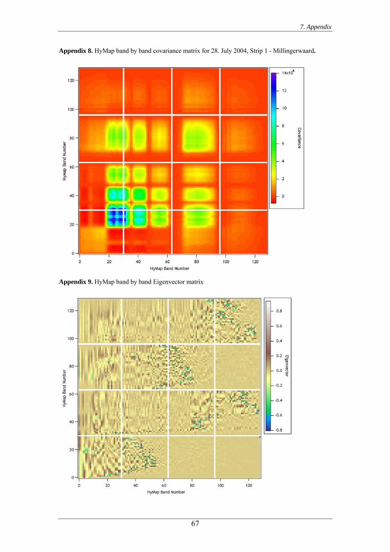
7. Appendix

Appendix 8. HyMap band by band covariance matrix for 28. July 2004, Strip 1 - Millingerwaard.

Appendix 9. HyMap band by band Eigenvector matrix

67

7. Appendix

Appendix 10. HyMap Quicklook ‘Millingerwaard’, 28. July 2004, Strip 1 (RGB = 15/10/5 (652.6 nm, 576.3 nm, 500.1 nm)) (left = Raw DLR quicklook, right = Geocoded and calibrated VITO quicklook).

68

validation of ground biophysical products using imaging

Documents