validation of the dynamic core of the palm model system 6

Validation of the Dynamic Core of the PALM Model System 6.0 inUrban Environments: LES and Wind-tunnel ExperimentsTobias Gronemeier1, Kerstin Surm2, Frank Harms2, Bernd Leitl2, Björn Maronga1,3, andSiegfried Raasch1

1Leibniz University Hannover, Institute of Meteorology and Climatology, Hannover, Germany2Universität Hamburg, Meteorological Institute, Hamburg, Germany3University of Bergen, Geophysical Institute, Bergen, Norway

Correspondence: Tobias Gronemeier ([email protected])

Abstract. We present the capability of PALM 6.0, the latest version of the PALM model system, to simulate neutrally stratified

urban boundary layers. The studied situation includes a real-case building setup of the HafenCity area in Hamburg, Ger-

many. Simulation results are validated against wind-tunnel measurements of the same building layout utilizing PALM’s virtual

measurement module. The comparison reveals an overall very high agreement between simulation results and wind-tunnel

measurements not only for mean wind speed and direction but also for turbulence statistics. However, differences between5

measurements and simulation arise within close vicinity of surfaces where the resolution prevents good representation of the

inertial sub-range of turbulence. In the end, we give guidance how these differences can be reduced using already implemented

features of PALM.

1 Introduction

The PALM model system version 6.0 is the latest version of the computational fluid-dynamics (CFD) model PALM, a Fortran10

based code to simulate atmospheric and oceanic boundary layers. Version 6.0 was developed within the scope of the Urban

Climate Under Change ([UC]2) framework funded by the German Federal Ministry of Education and Research (Scherer et al.,

2019; Maronga et al., 2019). The aim of the [UC]2 project is to develop a fully functional urban climate model capable of

simulating the urban canopy layer from city scale down to building scale with grid sizes down to 1 m or less. A detailed

description of the model system is given by Maronga et al. (2015, 2020). PALM has already been applied to a variety of15

studies within the area of urban boundary-layer research (e.g., Letzel et al., 2008; Park et al., 2012; Kanda et al., 2013; Kurppa

et al., 2018; Wang and Ng, 2018; Paas et al., 2020). Built upon PALM version 4.0, the latest version 6.0 contains many

new features and improvements of already existing components of the model system. One of the most impacting changes is

the new treatment of surfaces within PALM. While PALM did not distinguish between different surface types within former

versions, it is now possible to directly specify a surface type to each individual solid surface within a model domain via the20

land-surface model (Maronga et al., 2020) or the building surface model (Resler et al., 2017; Maronga et al., 2020). Also, a

fully three-dimensional obstacle representation is possible while former versions allowed only a 2.5-dimensional representation

1

https://doi.org/10.5194/gmd-2020-172Preprint. Discussion started: 29 July 2020c© Author(s) 2020. CC BY 4.0 License.

of obstacles (no overhanging structures like bridges or gates). These additions, however, required extensive re-coding of the

former version PALM 4.0 which affected also the dynamic core of the model.

Whereas former versions of PALM were already validated against wind-tunnel measurements, real-world measurements,25

and other CFD codes (Letzel et al., 2008; Razak et al., 2013; Park et al., 2015b; Gronemeier and Sühring, 2019; Paas et al.,

2020), the drastic changes of PALM’s code base require a new validation from scratch. A sufficient validation is inevitable to

ensure confidence in the results of the PALM model system as it is also the case for every other CFD code (Blocken, 2015;

Oberkampf et al., 2004).

Because of the high complexity of PALM, validating the model is a very longsome and costly exercise and a complete30

validation of all model components would easily go beyond the scope of any article. Within this study, we therefore focus on

the validation of the model’s flow dynamics which make up the core of the model system and build the foundation for all other

features within PALM. In order to isolate the pure dynamics from all other code parts, PALM is operated in a pure dynamic

mode, i.e. all thermal effects (temperature and humidity distribution, radiation, surface albedo, heat capacity, etc) are switched

off. The simulation results can then be validated using wind-tunnel measurements (Leitl and Schatzmann, 2010) which are35

recorded in a similar setup as the simulation data. While it is virtually impossible to neglect temperature or humidity effects in

real-world measurements, wind-tunnel experiments can provide exactly the same idealized conditions as used in our idealized

simulation. Also, other difficulties such as additional non-resolved obstacles like trees or sub-grid features on building walls

existing in the real world can make a comparison with real-world measurements troublesome (Paas et al., 2020). Paas et al.

(2020) compared PALM simulations to measurements of a mobile measurement platform. Although overall good agreement40

was found between PALM and the measurements, some non-resolved obstacles like trees complicated the comparison at several

points and led to differences in results. Hence, we decided to validate PALM against an idealized wind-tunnel experiment for

this study.

A realistic building setup, in this case the HafenCity area of Hamburg, Germany, is chosen for validation. A real-case building

setup has the advantage over more idealized, i.e. a single-cube, cases that a variety of different building configurations, also45

including more or less solitary buildings, can be covered in a single simulation. Likewise, it may show the capability of PALM

to correctly reproduce a complex realistic wind distribution.

To further improve the quality of the validation, a blind test was conducted, i.e. both experiments (CFD and wind-tunnel)

were made independently from one another. Only information about the building layout and the inlet wind profile were shared

between both experiments. Such a blind test gives high value to the validation as no tweaking of either experiment is possible50

to tune the results towards each other. Although, there are methods to adjust CFD results to better match to measurements

(e.g., Blocken et al., 2007), these adjustments depend on the individual case and need to be re-calculated for each new studied

situation. Within this study, we chose not to utilize any adjustments to the results in order to show PALM’s capability to simulate

a certain situation without any customized correction of the results. Also, often, measurements might even be unavailable to

calculate such adjustment factors.55

2


2 Experimental setup

2.1 Wind-tunnel experiment

Measurements were carried out at the Environmental Wind Tunnel Laboratory (EWTL) facility ’WOTAN’ at University of

Hamburg, Germany. The 25 m long wind tunnel provides an 18 m long test section equipped with two turn tables and an

adjustable ceiling. The cross section of the tunnel measures 4 m in width and 3 m in height. Figure 1 shows a photograph60

from within the wind tunnel for reference. For each wind tunnel campaign, a neutrally stratified model boundary layer flow is

generated by a carefully optimized combination of turbulence generators at the inlet of the test section, and a compatible floor

roughness. For the present study a boundary layer flow was modelled to match full scale conditions for a typical urban boundary

layer measured at a 280 m tall tower in Billwerder, Hamburg. The mean wind profile can be described by a logarithmic

wind profile with a roughness length z0 = (0.66± 0.22)m and by a power law with a profile exponent α= 0.21± 0.02. The65

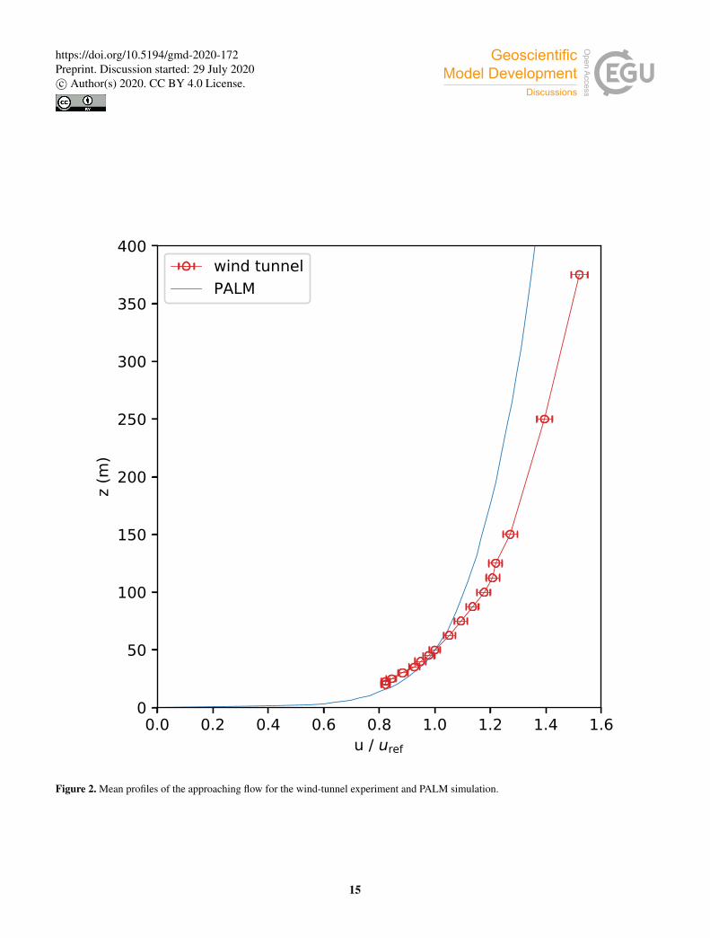
approaching flow profile is depicted in Fig. 2 and was modelled at a wind direction of 110◦.

A 2D Laser-Doppler-Anemometry (LDA) System was used to measure component-resolved flow data at sampling rates of

200 Hz–800 Hz (model scale), resolving even small-scale turbulence in time. At each measurement location a 3 minutes time

series was recorded which corresponds to a length of about 25 hours at full scale. The reference wind speed was permanently

monitored close to the tunnel inlet through Prandtl tube measurements. An area of 2.6km2 covering the HafenCity of Hamburg,70

Germany, was modelled at a scale of 1/500 within the wind tunnel (see Fig. 1). Measurements were taken at 25 different

locations within the building setup as shown in Fig. 3.

2.2 PALM simulation

The PALM Model System 6.0, revision 3921, was used to conduct the simulation for this study. PALM was operated using a

fifth-order advection scheme after Wicker and Skamarock (2002) in combination with a third-order Runge-Kutta timestepping75

scheme after (Williamson, 1980). At this point, we skip a detailed description of the PALM model. A detailed description

is provided by Maronga et al. (2015, 2020). For the PALM simulation, real-world scales were used. The simulation domain

covered an area of 6000 m by 2880 m horizontally and 601 m vertically at a spacial resolution of ∆x= ∆y = ∆z = 1m in

each direction. This resulted in about 10.4× 109 grid points for the used staggered Arakawa C grid (Harlow and Welch, 1965;

Arakawa and Lamb, 1977). The area of interest, i.e. the HafenCity area, was situated downstream of the simulation domain.80

The model domain was oriented so that the mean flow direction was aligned with x direction. With a mean wind direction of

110◦, the model was hence rotated counter-clockwise by 200◦.

The building layout as used in PALM is depicted in Fig. 4. In PALM, topography is considered using the mask method

(Briscolini and Santangelo, 1989) where a grid volume is either 100 % fluid or 100 % obstacle. In combination with PALM’s

rectilinear grid, this can cause buildings not aligned with the grid to appear differently, more brick-like, than they were within85

the wind tunnel.

The basic setup for this study is based on the settings used in the former study of Letzel et al. (2012).

3


A heterogeneous building setup usually requires a non-cyclic boundary condition along the mean flow direction to ensure

that building-generated turbulence is not cycled over and over the analysis area which otherwise might influence the results.

However, tests with non-cyclic boundary conditions along the mean flow showed that extremely long simulation times would be90

required to generate a stationary state. Hence, we used cyclic boundary conditions instead, which reduced the required CPU-

time significantly. The domain was extended in mean flow direction to allow the building-generated turbulence to dissipate

before the flow hits the target area again due to the cyclic conditions. As the simulation was aimed at a pure neutral case and

without releasing any trace gases or alike within the city area, there was no disadvantage in using cyclic boundary conditions

instead. After a simulation time of 7 h steady-state conditions were reached.95

At the top boundary, a fixed wind speed of 1.54 m s−1 was considered according to measurements within the wind tunnel

at the corresponding height. A constant flux layer was assumed between the surface and the first computational grid level to

calculate the surface shear stress, using a roughness length of z0 = 1m. Due to the staggered grid, the first computational level

is positioned 0.5∆z above the surface.

Within the wind-tunnel experiment, the modelled roughness length was z0 = (0.66± 0.22)m within the upstream area (cf.100

Sect. 2.1). With the chosen resolution of 1m this roughness length cannot be used in the PALM simulation, because it would

be larger than the assumed height of the constant flux layer (which is 0.5m) and hence would cause numerical problems. We

used a roughness length significantly smaller than half the grid spacing instead (i.e. z0� 0.5m), with a value of z0 = 0.1m

at each surface. Other comparable city simulations prove to give reasonable results using such value (e.g., Park et al., 2015a;

Gronemeier et al., 2017; Paas et al., 2020).105

To match the conditions within the wind tunnel, a strictly neutral atmosphere was considered with temperature being constant

over time. Also, the Coriolis force was neglected.

In the past, streak-like structures were reported for LES of neutral flows using cyclic boundary conditions (Munters et al.,

2016). To avoid such numerical artifacts, a shifting method was used according to Munters et al. (2016). The flow was shifted

by 300 m in y direction, i.e. perpendicular to the mean wind direction, before entering the domain at the left boundary.110

The wind field was initialized using a turbulent wind field from a precursor simulation via the cyclic-fill method (Maronga

et al., 2015). The setup of the precursor simulation was similar to the main simulation but with a reduced domain size of 600 m

by 600 m in horizontal direction. To initialize the precursor simulation, the approaching wind profile measured in the wind

tunnel was used as shown in Fig. 2.

The total simulation time of the main simulation was 12 h from which the first 7 h were required to reach a steady state of115

the simulation. The final 5 h were used for the analysis.

Figure 2 shows the mean wind profile of the flow approaching the building area during the analysis time. Differences between

the approaching flow within the wind tunnel and PALM are due to differences in the roughness of the upstream area. While

roughness elements were present within the wind-tunnel experiment, there were no such elements present within the PALM

simulation and surface roughness was considered only via the roughness length used within the constant-flux layer assumption120

at the lower-most grid level. Due to the mismatch in z0 as discussed above, the smoother surface within PALM causes higher

wind speed close to the ground and lower speed at greater heights. Antoniou et al. (2017) also reported a similar behaviour in

4


their comparison of LES and wind-tunnel results. Future simulations should hence try to include roughness elements similar

to those of the wind-tunnel to overcome this discrepancy.

2.3 Measurement stations125

Within the wind-tunnel experiments, wind speed was measured at certain measurement stations within the building array. The

locations of which are shown in Fig. 3. To be able to mirror the measurements as best as possible, the virtual measurement

module of PALM was used (Maronga et al., 2020). This module allows to define several virtual measurement stations within

the model domain via geographical coordinates. The model domain itself then needs to be geo-referenced in order to identify

the grid points closest to the measurement location. Referencing is done by assigning geographical coordinates and orientation130

to the lower left corner of the domain.

When mapping the measurement stations onto the PALM grid, there were two difficulties: First, there was not always

a grid point at the exact same location as the measurement points and therefore no data was available at the exact same

position; second, the topography in close vicinity of a measurement point might have been slightly different due to topography

representation used in PALM (cf. Sect. 2.2). To overcome these two issues, virtual measurements not only from the closest grid135

point to a measurement position were saved but also values from the neighbouring grid points. In post-processing, the area of

each measurement station was analyzed and a grid point selected which best fitted the wind-tunnel measurements.

At each measurement station presented in this study, nine profiles were recorded with a sampling rate between 2 Hz–2.5 Hz

(measurements recorded during each time step).

3 Results140

3.1 PALM simulation

The PALM simulation required a spin-up time of 7 h as can be seen by the time series of the domain-averaged kinetic energy

E = 0.5√u2 + v2 +w2 and the friction velocity u∗ (see Fig. 5). Both quantities stabilized after 7 h at around 0.8856m2 s−2

(E) and 0.0594ms−1 (u∗). Therefore, only data from the last 5 h of the simulation were used for the following validation.

The horizontally and time-averaged vertical profile of the stream-wise component of the vertical momentum flux wu is145

shown in Fig. 6. The vertical momentum flux wu can be split into a resolved and a subgrid-scale (SGS) part which is param-

eterized via an SGS model. The higher the resolved part, the less the SGS model contributes to the flux therefore indicating

that the flux and hence the turbulence causing the flux is well resolved. The ratio of the total, i.e. resolved plus SGS part,

momentum flux and its resolved part is close to 1 revealing that turbulence is properly resolved within the simulation domain

(see Fig. 6). At the surface, turbulence is less resolved due to the fact that turbulent structures tend to become smaller the closer150

they get to the surface and cannot be resolved by the grid spacing any more. However, the ratio between resolved and total wu

stays above 0.9 except for the lowest two grid levels.

5


To get an impression of the turbulent structures, Fig. 7 shows a snapshot of the magnitude of the rotation of the velocity field

as a measure of turbulence. One can clearly identify strong turbulent features (yellow and red structures) within the vicinity of

buildings while only weak turbulence is present above smooth surfaces.155

3.2 Comparison between wind-tunnel and PALM

To compare both experiments, results must to be normalized first as the experiments were conducted on different scales. The

reference wind speed uref used for normalization corresponds to the wind speed of the approaching flow at a height of 50 m

(real-world scale). In the following, results are given in real-world scales if not stated otherwise.

Figure 8 shows the wind distribution for each of these measurements at a height of 3 m and 2.5 m height above street level160

for (a) the wind-tunnel measurements and (b) the PALM simulation, respectively. Due to the staggered grid used in PALM

(cf. Sect. 2.2), PALM measurements are positioned 0.5 m lower than their corresponding wind-tunnel measurements. The

annotations give the normalized mean wind speed at the measurement location. Note, that measurement station 15 (cf. Fig. 3)

was positioned above a building of 18 m height and had, therefore, no values at 3 m and 10 m height. At most measurement

stations, the main wind direction is same in the PALM simulation compared to the wind-tunnel data.165

Largest differences of the wind distribution occur at station 6, 8, 13, and 20, where station 6 and 20 show a larger variation

in wind direction within the PALM simulation, and station 8 and 13 show different mean wind directions. On average, wind

speed is 23 % less in the PALM simulation compared to the wind-tunnel measurements.

The general lower wind speed recorded within PALM can be partly explained by the difference in measurement height.

Within PALM, measurements were located 0.5 m lower than in the wind-tunnel experiment due to the staggered Arakawa C170

grid (u and v values are calculated at half the height of each grid cell; given that ∆z = 1m, u and v are hence calculated

at heights of 0.5 m, 1.5 m, 2.5 m, and so on). This leads to overall lower wind speed especially close to the ground where

wind-speed gradients are large in relation to wind speed. Assuming a logarithmic wind profile, a height difference of 0.5 m

can result in 5.4 % lower wind speed at a height of 2.5 m. This error is reduced at greater height where wind-speed gradients

are smaller. However, Paas et al. (2020) also observed wind speeds being lower in PALM simulations compared to real-world175

measurements. The problem of low wind speed in PALM simulations observed in both studies, Paas et al. (2020) and ours,

might also be related to a mismatch in roughness length z0. For the comparison against real-world measurements done in Paas

et al. (2020), the used z0 might have over-estimated the wall roughness of the buildings, so as in our study, buildings might

have been smoother within the wind-tunnel experiment than estimated. The effect of z0-mismatch should be most pronounced

close to the surface and disappear at greater heights.180

At the next measurement height (wind tunnel: 10 m; PALM: 9.5 m), the mean wind speed is only 14 % less on average within

the PALM simulation (Fig. 9). Wind distribution is still very close between PALM and wind tunnel at most stations. While at

station 8, both experiments now show similar results, station 13 still records different wind direction and speed. Also, station 5

and 10 now show larger differences than at lower height. Still, at most measurement stations, PALM results agree with results

from the wind tunnel.185

6


At measurement heights 50 m and 75 m (not shown), PALM reports only 2 % and less than 1 % lower wind speed, respec-

tively, than the wind tunnel which supports the idea that a mismatch in z0 might be responsible for the differences.

The large discrepancy between PALM and the wind-tunnel results measured at station 13 can be explained by differences

within the building setup. Although the building data was checked thoroughly before the simulation, the windward building

at station 13 has different heights within the wind-tunnel experiment and the PALM simulation. While in the wind tunnel the190

building height is about 6 m, in PALM, it is set at 24 m (cf. Figs. 1 and 4). This leads to significant differences in the flow

around the building and hence causes different results at station 13. Wind direction and wind speed match again between

PALM and wind-tunnel measurements at heights above 30 m, i.e. above the building height (not shown).

The building layout was again thoroughly checked after discovering this flaw but no further deviations were detected within

the vicinity of any of the other measurement stations. A new simulation with an updated building height would yield different195

results around the changed building including station 13. However, given the fact that the local building configuration was

found to dominate the wind flow at the other measurement locations, it is very unlikely that the results would change in a

revised simulation. Therefore, repeating the simulation with an updated building layout around station 13 would not change

the overall outcome of the study.

In the following, we limit the discussion to three stations: 4, 11, and 7 which are chosen to represent a good, an average200

and a relatively poor agreement, respectively, between PALM and wind-tunnel measurements. Stations with similar results are

mentioned.

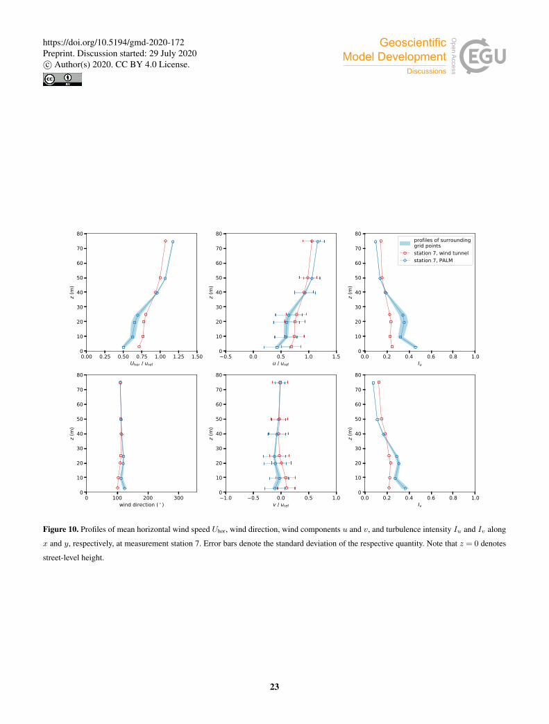
Figure 10 shows vertical profiles of the mean horizontal wind speed Uhor, wind direction, wind-vector components u and v,

as well as the turbulence intensity Iu and Iv along x- and y-direction, respectively, measured at station 7. Turbulence intensity

is defined as the ratio of standard deviation of the respective wind component and the mean horizontal wind speed. Error bars205

show the standard deviation of u and v measurements. The blue shaded area shows the range of values of all measured profiles

within PALM at that measurement station (at each station, profiles are measured at 9 neighboring locations, see Sect. 2.3).

Measurements present lower wind speed within the building canopy and higher wind speed above the canopy in PALM

compared to wind-tunnel measurements. Within the canopy, the flow is more turbulent in PALM as Iu and Iv are higher than

within the wind tunnel. This in turn leads to a reduced mean wind speed. The wind direction also differs slightly within the210

canopy. This all points to either a mismatch of measurement position where the PALM measurements might be placed not at

the exact same area within the edge flow at the building next to the measurement station; or the edge flow is of different shape

at station 7 due to different building resolution within the experiments. Stations 20, and 21 (not shown) show similar behaviour.

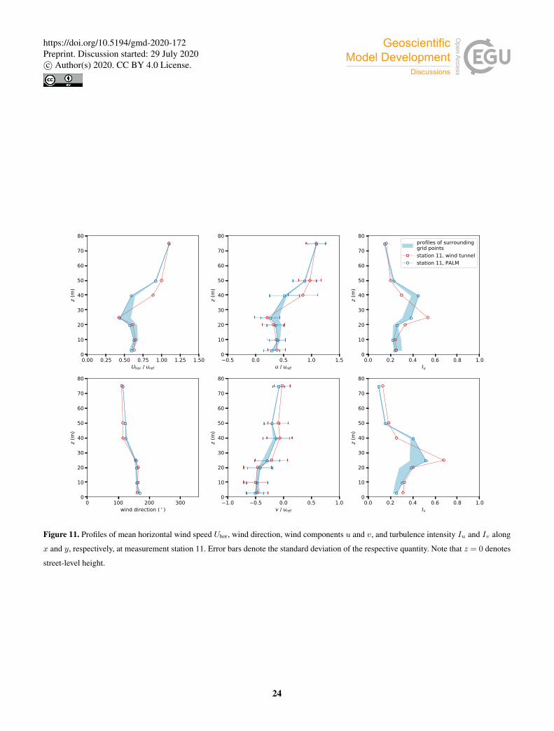
At station 11 (Fig. 11), variation in u and v are larger for the different profiles measured in PALM compared to station 7

which is shown by the larger blue-shaded area. This indicates that the wind field around station 11 varies stronger within the215

vicinity of the station compared to station 7. However, u and v and hence, Uhor and wind direction agree well between PALM

and wind-tunnel measurements. Larger differences occur in 40 m and 50 m height where PALM simulates lower wind speed

and slightly different wind directions. Turbulence intensity differs most at 25 m and 40 m height but agrees at other heights.

The rooftop of the surrounding buildings is at 26 m and 36 m height (cf. Fig. 4). Differences might therefore be related to

7


rooftop vortices being of slightly other shape within PALM compared to the wind tunnel. Results from stations 5, 6, 10, 15,220

and 17 are comparable to those of station 11.

Measurements at station 4 (Fig. 12) show a very close agreement between wind-tunnel and PALM results. The v profile

matches very well to that of the wind-tunnel measurement while the u values tend to be slightly lower than the wind-tunnel

measurement. This results in a good agreement of wind direction and horizontal wind speed as well. PALM does not only pro-

duce similar mean values as the wind tunnel experiment at station 4 but also the variance of wind speed and turbulence intensity225

matches well between wind-tunnel and PALM results. A similar agreement between PALM and wind-tunnel measurements

can be observed at the majority of stations, i.e. at stations 1–3, 8, 9, 12, 14, 16, 18, 19, 22–25.

A further insight of the simulated turbulence distribution is derived by analyzing the spectral energy density S. Figure 13

shows the dimensionless energy spectra for station 4 (left panel) and 11 (right panel) at different heights z. Spectra measured

at station 7 are comparable to those of station 11 and are therefore not shown. Note that the covered range of frequencies230

differ between PALM and wind-tunnel measurements as the sampling rate of the measurements and the measured time interval

vary between the PALM and wind-tunnel experiment. However, results of both experiments still overlap over a large range of

frequencies.

In general, spectra for both wind-vector components coincide to a high degree between PALM and wind-tunnel measure-

ments at all heights. The inertial range of the turbulence spectrum is clearly visible within both experiments at 75 m height235

(above the canopy layer) at both stations (Figs. 13a and b). The normalized energy spectrum decays with roughly f−23 fol-

lowing Kolmogorov’s theory. At high frequencies, spectra of the PALM measurements strongly decay which is related to

numerical dissipation and is a typical behaviour of LES models using high-order differencing schemes (e.g., Glendening and

Haack, 2001; Kitamura and Nishizawa, 2019).

At rooftop height (Figs. 13c and d), PALM’s spectra are shifted towards higher frequencies compared to those of the wind240

tunnel at the same height. This indicates that PALM simulates turbulence of smaller scales at these points. The effect is more

pronounced for station 4 than for station 11 and station 7 (not shown). The smaller turbulence within PALM might be due

to a higher roughness length z0 of the rooftops which in turn might either be due to the specified z0 being of too high value

or due to the increased roughness of the buildings introduced by the brick-like representation of the buildings in PALM (cf.

Sect. 2.2). Around station 7 and 11, building roofs are not flat but possess small additional structures which might give a higher245

roughness as a result of the grid-following topography structure in PALM compared to the building model within the wind-

tunnel experiment. This discrepancy then also leads to the difference already mentioned in the profiles of station 11 (Fig. 11).

At station 4, this effect is not as pronounced because the closest building to station 4 has a flat roof.

Spectra close to the surface again agree better between PALM and the wind tunnel measurements. Though, due to the

limited measurement frequency and very small turbulent structures at the surface, the inertial range is not covered by the wind-250

tunnel measurements at 3 m height. This height corresponds to the third grid level above the surface of the PALM simulation

and therefore it can be truly expected that the inertial range is only poorly resolved. Comparing the measured spectra to the

theoretical decay of fS ∝ f− 23 , the inertial range is indeed hardly represented within the data.

8


Results within the vicinity of the measurement stations could be improved by utilizing PALM’s self-nesting feature. This

allows to use a higher grid resolution within specific areas of the model domain. We recommend that future simulations should255

try using this feature for areas requiring high resolution.

4 Conclusions

In this study, we analyzed PALM’s capability to simulate a complex flow field within a realistic urban building array. Simulation

results were compared with measurements done at the EWTL facility at University of Hamburg, Germany. The aim was to

validate the dynamic core of the newest version 6.0 of PALM which underwent significant code-changes in recent model260

development.

The comparison of PALM results with the wind tunnel data proves that the model can correctly simulate a neutrally stratified

urban boundary layer produced by a realistic complex building array. Measurements were compared at several different posi-

tions throughout the building array at non-obstructed locations, at the windward and leeward site of buildings as well as within

street canyons and at intersections. Overall, the PALM results highly agreed with the corresponding wind-tunnel measurements265

in regards to wind speed and direction as well as turbulence intensity. Differences could be observed close to surfaces where

PALM reported slightly lower wind speed compared to wind-tunnel measurements. Such discrepancies were also reported

recently by Paas et al. (2020) when comparing PALM simulations to real-world measurements. These differences can to large

extent be ascribed to deficiencies in the model setup, namely the choice of a relatively large and homogeneous roughness

length in the whole model domain, which creates excessive turbulence and a reduced mean wind in the vicinity of buildings.270

Our choice of z0 = 0.1m is also not consistent with the recommendations given by Basu and Lacser (2017) who recommend

that the first grid level should at least be at 50z0. Given that the first computational grid level is set at 0.5m, z0 should have

been no larger than 0.01m which could have also better resembled the smooth surface of the buildings within the wind-tunnel

experiment. An improved simulation setup would have to set a significantly smaller z0 within the building array to improve the

wind field close to the surface. To also resemble a rough surface within the upstream area, roughness elements similar to those275

from the wind-tunnel experiment should then be simulated as well. Moreover, changes in the measurement heights between

wind tunnel and LES led to systematic differences, particularly near the surface where the vertical wind gradients are large.

When planning a simulation, it must be taken into consideration, that surfaces are always aligned with the rectilinear grid

within PALM. If the alignment of walls and the simulation grid do not match, the resulting brick-like representation can lead

to a higher surface roughness and hence to higher turbulence presumably altering the results and leading to differences to other280

measurements. To overcome this error or at least reduce its effect, a higher grid resolution should be used which will then

minimize the size of artificially created steps for topography elements non-aligned to the numerical grid. In order to achieve

this without increasing the computational costs significantly, PALM’s ability of grid nesting should be used.

In the present study, we also experienced that input data must always be checked with very high caution. Especially large

building data sets might contain errors and false building heights or missing/displaced buildings, which are more difficult285

to spot than in setups with a limited number of buildings. This is, of course, of utmost importance for the area-of-interest,

9


but also the upwind region requires proper verification as it directly affects the analysis area. Also, when comparing to other

experiments like real-world or wind-tunnel measurements, positioning of the measurements must be thoroughly checked as

mentioned by Paas et al. (2020). This is also true for positioning virtual measurements within the PALM domain. At positions

with highly complex wind fields, it can make a large difference for the results if measurement positions are off by only a single290

grid point (as can be seen, e.g., by the range of profiles for station 11, Fig. 11). This of course depends strongly on the grid

spacing used and will be most relevant when using relatively coarse grids.

This study focused only on a single but the most essential part of PALM, the dynamic core. However, validation of the

entire model requires additional studies focusing on the other model parts like the radiation module, the chemistry module or

the land-surface module to mention only a few. Some of these are already validated (Resler et al., 2017; Kurppa et al., 2019;295

Fröhlich and Matzarakis, 2019), others will follow in future publications.

Code and data availability. The PALM model system is freely available from http://palm-model.org and distributed under the GNU General

Public License v3 (http://www.gnu.org/copyleft/gpl.html). The model source code of version 6.0 in revision 3921, used in this article, is

archived on the Research Data Repository of the Leibniz University of Hannover (Gronemeier et al., 2020b) as well as input data and

measurement results presented in this paper in combination with plotting scripts to reproduce the presented figures (Gronemeier et al.,300

2020a).

Author contributions. BL and KS created the wind-tunnel setup. KS conducted the wind-tunnel measurements and analysis with supervision

of FH and BL. TG, SR and BM created the simulation setup. TG carried out the simulations and precursor test simulations with supervision

of SR. All authors took part in data analysis of the comparison. TG compiled the manuscript with contributions by all coauthors.

Competing interests. The authors declare that no competing interests are present.305

Acknowledgements. We like to thank everyone who helped to conduct the experiments and helped by writing software for the analysis of

the results (including data preparation, model building, and code bug-fixing). This study was part of the [UC]2 project which is funded by

the German Federal Ministry of Education and Research (BMBF) within the framework ’Research for Sustainable Development’ (FONA;

www.fona.de). It was conducted in collaboration of the two sub-projects MOSAIK (funding code: 01LP1601) and 3DO (funding code:

01LP1602). The authors would like to thank Wieke Heldens and Julian Zeidler at the German Aerospace Center (DLR) for the support310

during the project and especially for building-data preparation used within this study. All simulations were carried out on the computer

clusters of the North-German Supercomputing Alliance (HLRN; www.hlrn.de). Data analysis was done using Python.

10


References

Antoniou, N., Montazeri, H., Wigo, H., Neophytou, M. K.-A., Blocken, B., and Sandberg, M.: CFD and Wind-Tunnel Analysis of Outdoor

Ventilation in a Real Compact Heterogeneous Urban Area: Evaluation Using “Air Delay”, Building and Environment, 126, 355–372,315

https://doi.org/10.1016/j.buildenv.2017.10.013, 2017.

Arakawa, A. and Lamb, V. R.: Computational Design of the Basic Dynamical Processes of the UCLA General Circulation Model, in: General

Circulation Models of the Atmosphere, vol. 17, pp. 173–265, Methods in computational Physics, edited by: Chang, J., 1977.

Basu, S. and Lacser, A.: A Cautionary Note on the Use of Monin–Obukhov Similarity Theory in Very High-Resolution Large-Eddy Simula-

tions, Boundary-Layer Meteorol, 163, 351–355, https://doi.org/10.1007/s10546-016-0225-y, 2017.320

Blocken, B.: Computational Fluid Dynamics for Urban Physics: Importance, Scales, Possibilities, Limitations and Ten Tips and Tricks to-

wards Accurate and Reliable Simulations, Building and Environment, 91, 219–245, https://doi.org/10.1016/j.buildenv.2015.02.015, 2015.

Blocken, B., Carmeliet, J., and Stathopoulos, T.: CFD Evaluation of Wind Speed Conditions in Passages between Parallel Buildings—Effect

of Wall-Function Roughness Modifications for the Atmospheric Boundary Layer Flow, Journal of Wind Engineering and Industrial Aero-

dynamics, 95, 941–962, https://doi.org/10.1016/j.jweia.2007.01.013, 2007.325

Briscolini, M. and Santangelo, P.: Development of the Mask Method for Incompressible Unsteady Flows, J. Comp. Phys., 84, 57–75,

https://doi.org/10.1016/0021-9991(89)90181-2, 1989.

Fröhlich, D. and Matzarakis, A.: Calculating Human Thermal Comfort and Thermal Stress in the PALM Model System 6.0, Geosci. Model

Dev. Discuss., 2019, 1–21, https://doi.org/10.5194/gmd-2019-202, in review, 2019.

Glendening, J. W. and Haack, T.: Influence Of Advection Differencing Error Upon Large-Eddy Simulation Accuracy, Boundary-Layer330

Meteorol, 98, 127–153, https://doi.org/10.1023/A:1018734205850, 2001.

Gronemeier, T. and Sühring, M.: On the Effects of Lateral Openings on Courtyard Ventilation and Pollution—A Large-Eddy Simulation

Study, Atmosphere, 10, 63, https://doi.org/10.3390/atmos10020063, 2019.

Gronemeier, T., Raasch, S., and Ng, E.: Effects of Unstable Stratification on Ventilation in Hong Kong, Atmosphere, 8, 168,

https://doi.org/10.3390/atmos8090168, 2017.335

Gronemeier, T., Surm, K., Harms, F., Leitl, B., Maronga, B., and Raasch, S.: Dataset: Validation of the Dynamic Core of the PALM Model

System 6.0 in Urban Environments: Simulation Input Data and Measurement Data, https://doi.org/10.25835/0015082, 2020a.

Gronemeier, T. et al.: Dataset: PALM 6.0 r3921, https://doi.org/10.25835/0046914, 2020b.

Harlow, F. H. and Welch, J. E.: Numerical Calculation of Time-Dependent Viscous Incompressible Flow of Fluid with Free Surface, Phys.

Fluids, 8, 2182, https://doi.org/10.1063/1.1761178, 1965.340

Kanda, M., Inagaki, A., Miyamoto, T., Gryschka, M., and Raasch, S.: A New Aerodynamic Parametrization for Real Urban Surfaces,

Boundary-Layer Meteorol, 148, 357–377, https://doi.org/10.1007/s10546-013-9818-x, 2013.

Kitamura, Y. and Nishizawa, S.: Estimation of Energy Dissipation Caused by Odd Order Difference Schemes for an Unstable Planetary

Boundary Layer, Atmos Sci Lett, 20, e905, https://doi.org/10.1002/asl.905, 2019.

Kurppa, M., Hellsten, A., Auvinen, M., Raasch, S., Vesala, T., and Järvi, L.: Ventilation and Air Quality in City Blocks Using Large-Eddy345

Simulation—Urban Planning Perspective, Atmosphere, 9, 65, https://doi.org/10.3390/atmos9020065, 2018.

Kurppa, M., Hellsten, A., Roldin, P., Kokkola, H., Tonttila, J., Auvinen, M., Kent, C., Kumar, P., Maronga, B., and Järvi, L.: Implementation

of the Sectional Aerosol Module SALSA2.0 into the PALM Model System 6.0: Model Development and First Evaluation, Geosci. Model

Dev., 12, 1403–1422, https://doi.org/10.5194/gmd-12-1403-2019, 2019.

11


Leitl, B. and Schatzmann, M.: Validation Data for Urban Flow and Dispersion Models - Are Wind Tunnel Data Qualified?, in: The Fifth350

International Symposium on Computational Wind Engineering (CWE2010), p. 8, Chapel Hill, North Carolina, USA, 2010.

Letzel, M. O., Krane, M., and Raasch, S.: High Resolution Urban Large-Eddy Simulation Studies from Street Canyon to Neighbourhood

Scale, Atmospheric Environment, 42, 8770–8784, https://doi.org/10.1016/j.atmosenv.2008.08.001, 2008.

Letzel, M. O., Helmke, C., Ng, E., An, X., Lai, A., and Raasch, S.: LES Case Study on Pedestrian Level Ventilation in Two Neighbourhoods

in Hong Kong, Meteorol. Z., 21, 575–589, https://doi.org/10.1127/0941-2948/2012/0356, 2012.355

Li, S., Jaroszynski, S., Pearse, S., Orf, L., and Clyne, J.: VAPOR: A Visualization Package Tailored to Analyze Simulation Data in Earth

System Science, Atmosphere, 10, https://doi.org/10.3390/atmos10090488, 2019.

Maronga, B., Gryschka, M., Heinze, R., Hoffmann, F., Kanani-Sühring, F., Keck, M., Ketelsen, K., Letzel, M. O., Sühring, M., and Raasch,

S.: The Parallelized Large-Eddy Simulation Model (PALM) Version 4.0 for Atmospheric and Oceanic Flows: Model Formulation, Recent

Developments, and Future Perspectives, Geosci. Model Dev., 8, 2515–2551, https://doi.org/10.5194/gmd-8-2515-2015, 2015.360

Maronga, B., Gross, G., Raasch, S., Banzhaf, S., Forkel, R., Heldens, W., Kanani-Sühring, F., Matzarakis, A., Mauder, M., Pavlik, D., Pfaf-

ferott, J., Schubert, S., Seckmeyer, G., Sieker, H., and Winderlich, K.: Development of a New Urban Climate Model Based on the Model

PALM – Project Overview, Planned Work, and First Achievements, Meteorol. Z., 28, 105–119, https://doi.org/10.1127/metz/2019/0909,

2019.

Maronga, B., Banzhaf, S., Burmeister, C., Esch, T., Forkel, R., Fröhlich, D., Fuka, V., Gehrke, K. F., Geletic, J., Giersch, S., Gronemeier, T.,365

Groß, G., Heldens, W., Hellsten, A., Hoffmann, F., Inagaki, A., Kadasch, E., Kanani-Sühring, F., Ketelsen, K., Khan, B. A., Knigge, C.,

Knoop, H., Krc, P., Kurppa, M., Maamari, H., Matzarakis, A., Mauder, M., Pallasch, M., Pavlik, D., Pfafferott, J., Resler, J., Rissmann,

S., Russo, E., Salim, M., Schrempf, M., Schwenkel, J., Seckmeyer, G., Schubert, S., Sühring, M., von Tils, R., Vollmer, L., Ward, S.,

Witha, B., Wurps, H., Zeidler, J., and Raasch, S.: Overview of the PALM Model System 6.0, Geosci. Model Dev., 13, 1335–1372,

https://doi.org/10.5194/gmd-13-1335-2020, 2020.370

Munters, W., Meneveau, C., and Meyers, J.: Shifted Periodic Boundary Conditions for Simulations of Wall-Bounded Turbulent Flows,

Physics of Fluids, 28, 025 112, https://doi.org/10.1063/1.4941912, 2016.

Oberkampf, W. L., Trucano, T. G., and Hirsch, C.: Verification, Validation, and Predictive Capability in Computational Engineering and

Physics, Applied Mechanics Reviews, 57, 345–384, https://doi.org/10.1115/1.1767847, 2004.

Paas, B., Zimmermann, T., and Klemm, O.: Analysis of a Turbulent Wind Field in a Street Canyon: Good Agreement between LES Model375

Results and Data from a Mobile Platform, Meteorol. Z., p. 93256, https://doi.org/10.1127/metz/2020/1006, 2020.

Park, S.-B., Baik, J.-J., Raasch, S., and Letzel, M. O.: A Large-Eddy Simulation Study of Thermal Effects on Turbulent Flow and Dispersion

in and above a Street Canyon, J. Appl. Meteor. Climatol., 51, 829–841, https://doi.org/10.1175/JAMC-D-11-0180.1, 2012.

Park, S.-B., Baik, J.-J., and Han, B.-S.: Large-Eddy Simulation of Turbulent Flow in a Densely Built-up Urban Area, Environ Fluid Mech,

15, 235–250, https://doi.org/10.1007/s10652-013-9306-3, 2015a.380

Park, S.-B., Baik, J.-J., and Lee, S.-H.: Impacts of Mesoscale Wind on Turbulent Flow and Ventilation in a Densely Built-up Urban Area, J.

Appl. Meteor. Climatol., 54, 811–824, https://doi.org/10.1175/JAMC-D-14-0044.1, 2015b.

Razak, A. A., Hagishima, A., Ikegaya, N., and Tanimoto, J.: Analysis of Airflow over Building Arrays for Assessment of Urban Wind

Environment, Building and Environment, 59, 56–65, https://doi.org/10.1016/j.buildenv.2012.08.007, 2013.

Resler, J., Krc, P., Belda, M., Juruš, P., Benešová, N., Lopata, J., Vlcek, O., Damašková, D., Eben, K., Derbek, P., Maronga, B., and Kanani-385

Sühring, F.: PALM-USM v1.0: A New Urban Surface Model Integrated into the PALM Large-Eddy Simulation Model, Geosci. Model

Dev., 10, 3635–3659, https://doi.org/10.5194/gmd-10-3635-2017, 2017.

12


Scherer, D., Antretter, F., Bender, S., Cortekar, J., Emeis, S., Fehrenbach, U., Gross, G., Halbig, G., Hasse, J., Maronga, B., Raasch, S., and

Scherber, K.: Urban Climate Under Change [UC]2 – A National Research Programme for Developing a Building-Resolving Atmospheric

Model for Entire City Regions, Meteorol. Z., 28, 95–104, https://doi.org/10.1127/metz/2019/0913, 2019.390

Wang, W. and Ng, E.: Air Ventilation Assessment under Unstable Atmospheric Stratification — A Comparative Study for Hong Kong,

Building and Environment, 130, 1–13, https://doi.org/10.1016/j.buildenv.2017.12.018, 2018.

Wicker, L. J. and Skamarock, W. C.: Time-Splitting Methods for Elastic Models Using Forward Time Schemes, MONTHLY WEATHER

REVIEW, 130, 10, 2002.

Williamson, J.: Low-Storage Runge-Kutta Schemes, Journal of Computational Physics, 35, 48–56, https://doi.org/10.1016/0021-395

9991(80)90033-9, 1980.

13


Figure 1. Photograph of the building setup within the wind-tunnel facility ’WOTAN’ for an approaching flow of 290◦. Please note that

contrary to the depicted orientation, an approaching flow from 110◦ was used within this study.

14


0.0 0.2 0.4 0.6 0.8 1.0 1.2 1.4 1.6u / uref

0

50

100

150

200

250

300

350

400

z (m

)

wind tunnelPALM

Figure 2. Mean profiles of the approaching flow for the wind-tunnel experiment and PALM simulation.

15


N

Figure 3. Building layout used in the wind-tunnel experiment. Measurement locations are marked and labeled by their respective number.

16


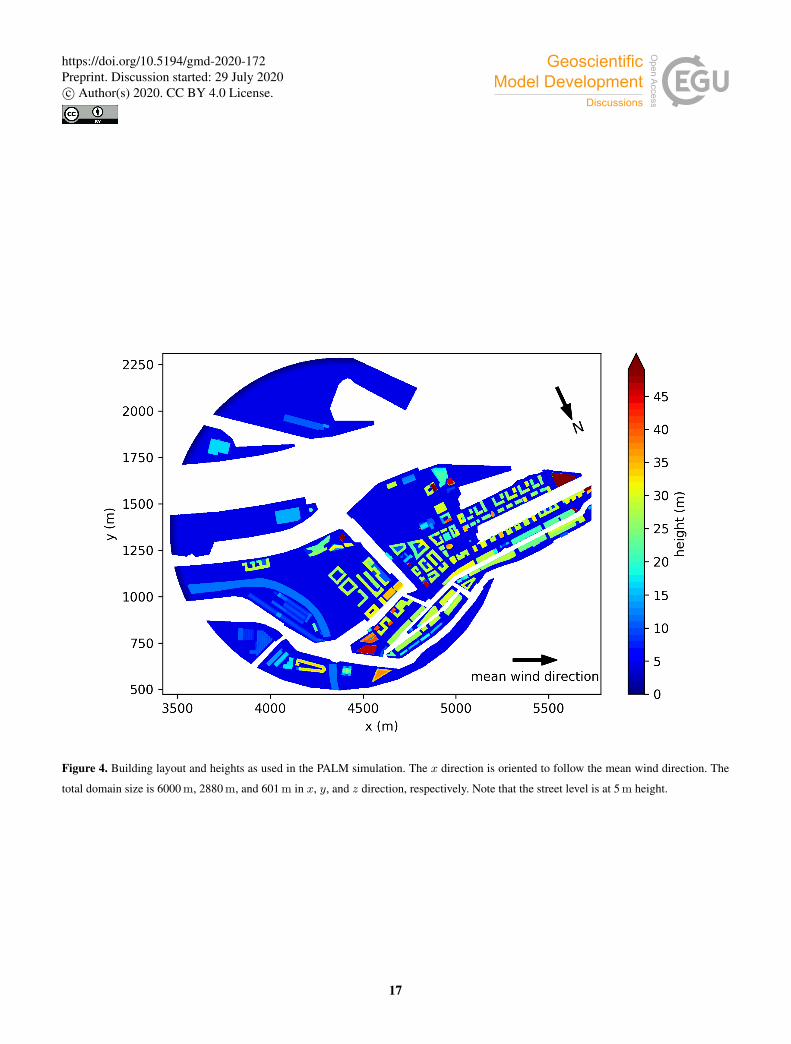
Figure 4. Building layout and heights as used in the PALM simulation. The x direction is oriented to follow the mean wind direction. The

total domain size is 6000 m, 2880 m, and 601 m in x, y, and z direction, respectively. Note that the street level is at 5 m height.

17


0 2 4 6 8 10 12time (h)

0.885

0.890

0.895

0.900

E (m

2 s2 )

0 2 4 6 8 10 12time (h)

0.055

0.060

u * (m

s1 )

Figure 5. Time series of the total kinetic energy E and the friction velocity u∗ of the PALM simulation.

18


0.004 0.003 0.002 0.001 0.000wu / u2

ref

0

50

100

150

200

250

300

350

400

z (m

)

total fluxresolved / total

0.0 0.2 0.4 0.6 0.8 1.0ratio

Figure 6. Mean profile of the vertical momentum flux and the ratio between resolved and total flux, averaged over the entire domain of the

PALM simulation.

19


Figure 7. View of the volume-rendered instantaneous turbulence structures above the building array. Turbulence is visualized using the

magnitude of the rotation of the velocity field. Green and red colour show low and high values, respectively. Image was rendered using

VAPOR (Li et al., 2019).

20


mean wind direction

0 - 0.20.2 - 0.40.4 - 0.60.6 - 0.80.8 - 1.01.0 - 1.21.2 - 1.4> 1.4

N

mean wind direction

0 - 0.20.2 - 0.40.4 - 0.60.6 - 0.80.8 - 1.01.0 - 1.21.2 - 1.4> 1.4

N

(a)

(b)

Figure 8. Wind-speed distribution at all measurement stations at 3 m height above street level for (a) wind-tunnel measurements and (b) the

PALM simulation.

21


mean wind direction

0 - 0.20.2 - 0.40.4 - 0.60.6 - 0.80.8 - 1.01.0 - 1.21.2 - 1.4> 1.4

N

mean wind direction

0 - 0.20.2 - 0.40.4 - 0.60.6 - 0.80.8 - 1.01.0 - 1.21.2 - 1.4> 1.4

N

(a)

(b)

Figure 9. Wind-speed distribution at all measurement stations at 10 m height above street level for (a) wind-tunnel measurements and (b) the

PALM simulation.

22


0.00 0.25 0.50 0.75 1.00 1.25 1.50Uhor / uref

0

10

20

30

40

50

60

70

80

z (m

)

0.5 0.0 0.5 1.0 1.5u / uref

0

10

20

30

40

50

60

70

80

z (m

)

0.0 0.2 0.4 0.6 0.8 1.0Iu

0

10

20

30

40

50

60

70

80

z (m

)

profiles of surroundinggrid pointsstation 7, wind tunnelstation 7, PALM

0 100 200 300wind direction ( )

0

10

20

30

40

50

60

70

80

z (m

)

1.0 0.5 0.0 0.5 1.0v / uref

0

10

20

30

40

50

60

70

80

z (m

)

0.0 0.2 0.4 0.6 0.8 1.0Iv

0

10

20

30

40

50

60

70

80

z (m

)

Figure 10. Profiles of mean horizontal wind speed Uhor, wind direction, wind components u and v, and turbulence intensity Iu and Iv along

x and y, respectively, at measurement station 7. Error bars denote the standard deviation of the respective quantity. Note that z = 0 denotes

street-level height.

23


0.00 0.25 0.50 0.75 1.00 1.25 1.50Uhor / uref

0

10

20

30

40

50

60

70

80

z (m

)

0.5 0.0 0.5 1.0 1.5u / uref

0

10

20

30

40

50

60

70

80

z (m

)

0.0 0.2 0.4 0.6 0.8 1.0Iu

0

10

20

30

40

50

60

70

80

z (m

)



0

10

20

30

40

50

60

70

80

z (m

)

1.0 0.5 0.0 0.5 1.0v / uref

0

10

20

30

40

50

60

70

80

z (m

)

0.0 0.2 0.4 0.6 0.8 1.0Iv

0

10

20

30

40

50

60

70

80

z (m

)




24


0.00 0.25 0.50 0.75 1.00 1.25 1.50Uhor / uref

0

10

20

30

40

50

60

70

80

z (m

)

0.5 0.0 0.5 1.0 1.5u / uref

0

10

20

30

40

50

60

70

80

z (m

)

0.0 0.2 0.4 0.6 0.8 1.0Iu

0

10

20

30

40

50

60

70

80

z (m

)



0

10

20

30

40

50

60

70

80

z (m

)

1.0 0.5 0.0 0.5 1.0v / uref

0

10

20

30

40

50

60

70

80

z (m

)

0.0 0.2 0.4 0.6 0.8 1.0Iv

0

10

20

30

40

50

60

70

80

z (m

)




25


10 5

10 4

10 3

10 2

10 1

100

fS

2

(a)z = 75 m

station 4

f 2/3

u (wind tunnel)v (wind tunnel)u (PALM)v (PALM)

(b)z = 75 m

station 11

prof

ile to

p

10 5

10 4

10 3

10 2

10 1

100

fS

2

(c)z = 20 m

(d)z = 40 m

roof

top

10 4 10 3 10 2 10 1 100 101 102 103

f z U 1hor

10 5

10 4

10 3

10 2

10 1

100

fS

2

(e)z = 3 m

10 4 10 3 10 2 10 1 100 101 102 103

f z U 1hor

(f)z = 3 m

surfa

ce

Figure 13. Spectral energy density S for u and v at station 4 (left) and station 11 (right) at profile top (a, b), rooftop height (c, d), and at the

surface (e, f). S is normalized by multiplying with the frequency f and dividing by the variance σ2. For reference, f−23 indicating the slope

of energy decay according to Kolmogorov’s theory is added to the plots. Note that z is given relative to street-level height.

26


validation of the dynamic core of the palm model system 6

Documents