valuation of basket credit derivatives in the credit migrations … · 2016-02-09 · valuation of...
TRANSCRIPT
VALUATION OF BASKET CREDIT DERIVATIVES IN
THE CREDIT MIGRATIONS ENVIRONMENT
Tomasz R. Bielecki∗
Department of Applied Mathematics
Illinois Institute of Technology
Chicago, IL 60616, USA
Stephane Crepey†
Departement de Mathematiques
Universite d’Evry Val d’Essonne
91025 Evry Cedex, France
Monique Jeanblanc‡
Departement de Mathematiques
Universite d’Evry Val d’Essonne
91025 Evry Cedex, France
Marek Rutkowski§
School of Mathematics
University of New South Wales
Sydney, NSW 2052, Australia
and
Faculty of Mathematics and Information Science
Warsaw University of Technology
00-661 Warszawa, Poland
Abstract
The goal of this work is to present a methodology aimed at valuation and hedging of basketcredit derivatives, as well as of portfolios of credits/loans, in the context of several possible creditratings of underlying credit instruments. The methodology is based on a specific Markovianmodel of a financial market.
∗The research of T.R. Bielecki was supported by NSF Grant 0202851 and Moody’s Corporation grant 5-55411.†The research of S. Crepey was supported by Zeliade‡The research of M. Jeanblanc was supported by Zeliade and Moody’s Corporation grant 5-55411.§The research of M. Rutkowski was supported by the 2005 Faculty Research Grant PS06987.
1
2 Valuation of Basket Credit Derivatives
Contents
1 Introduction 3
1.1 Conditional Expectations Associated with Credit Derivatives . . . . . . . . . . . . . . . . . . 3
1.2 Existing Methods of Modelling Dependent Defaults . . . . . . . . . . . . . . . . . . . . . . . . 5
2 Notation and Preliminary Results 6
2.1 Credit Migrations . . . . . . . . . . . . . . . . . . . . . . . . . . . . . . . . . . . . . . . . . . . 6
2.1.1 Markovian Set-up . . . . . . . . . . . . . . . . . . . . . . . . . . . . . . . . . . . . . . 7
2.2 Conditional Expectations . . . . . . . . . . . . . . . . . . . . . . . . . . . . . . . . . . . . . . 7
2.2.1 Markovian Case . . . . . . . . . . . . . . . . . . . . . . . . . . . . . . . . . . . . . . . 9
3 Markovian Market Model 9
3.1 Specification of Credit Ratings Transition Intensities . . . . . . . . . . . . . . . . . . . . . . . 11
3.2 Conditionally Independent Migrations . . . . . . . . . . . . . . . . . . . . . . . . . . . . . . . 12
4 Changes of Measures and Markovian Numeraires 12
4.1 Markovian Change of a Probability Measure . . . . . . . . . . . . . . . . . . . . . . . . . . . . 12
4.2 Markovian Numeraires and Valuation Measures . . . . . . . . . . . . . . . . . . . . . . . . . . 14
4.3 Examples of Markov Market Models . . . . . . . . . . . . . . . . . . . . . . . . . . . . . . . . 15
4.3.1 Markov Chain Migration Process . . . . . . . . . . . . . . . . . . . . . . . . . . . . . . 15
4.3.2 Diffusion-type Factor Process . . . . . . . . . . . . . . . . . . . . . . . . . . . . . . . . 16
4.3.3 CDS Spread Factor Model . . . . . . . . . . . . . . . . . . . . . . . . . . . . . . . . . . 16
5 Valuation of Single Name Credit Derivatives 17
5.1 Survival Claims . . . . . . . . . . . . . . . . . . . . . . . . . . . . . . . . . . . . . . . . . . . . 17
5.2 Credit Default Swaps . . . . . . . . . . . . . . . . . . . . . . . . . . . . . . . . . . . . . . . . . 17
5.2.1 Default Payment Leg . . . . . . . . . . . . . . . . . . . . . . . . . . . . . . . . . . . . . 18
5.2.2 Premium Payment Leg . . . . . . . . . . . . . . . . . . . . . . . . . . . . . . . . . . . . 18
5.3 Forward CDS . . . . . . . . . . . . . . . . . . . . . . . . . . . . . . . . . . . . . . . . . . . . . 18
5.3.1 Default Payment Leg . . . . . . . . . . . . . . . . . . . . . . . . . . . . . . . . . . . . . 19
5.3.2 Premium Payment Leg . . . . . . . . . . . . . . . . . . . . . . . . . . . . . . . . . . . . 19
5.4 CDS Swaptions . . . . . . . . . . . . . . . . . . . . . . . . . . . . . . . . . . . . . . . . . . . . 19
5.4.1 Conditionally Gaussian Case . . . . . . . . . . . . . . . . . . . . . . . . . . . . . . . . 20
6 Valuation of Basket Credit Derivatives 20
6.1 kth-to-default CDS . . . . . . . . . . . . . . . . . . . . . . . . . . . . . . . . . . . . . . . . . . 21
6.1.1 Default Payment Leg . . . . . . . . . . . . . . . . . . . . . . . . . . . . . . . . . . . . . 21
6.1.2 Premium Payment Leg . . . . . . . . . . . . . . . . . . . . . . . . . . . . . . . . . . . . 22
6.2 Forward kth-to-default CDS . . . . . . . . . . . . . . . . . . . . . . . . . . . . . . . . . . . . . 22
6.2.1 Default Payment Leg . . . . . . . . . . . . . . . . . . . . . . . . . . . . . . . . . . . . . 22
6.2.2 Premium Payment Leg . . . . . . . . . . . . . . . . . . . . . . . . . . . . . . . . . . . . 22
7 Model Implementation 23
7.1 Curse of Dimensionality . . . . . . . . . . . . . . . . . . . . . . . . . . . . . . . . . . . . . . . 23
7.2 Recursive Simulation Procedure . . . . . . . . . . . . . . . . . . . . . . . . . . . . . . . . . . . 23
7.2.1 Simulation Algorithm: Special Case . . . . . . . . . . . . . . . . . . . . . . . . . . . . 24
7.3 Estimation and Calibration of the Model . . . . . . . . . . . . . . . . . . . . . . . . . . . . . . 26
7.4 Portfolio Credit Risk . . . . . . . . . . . . . . . . . . . . . . . . . . . . . . . . . . . . . . . . . 26

T.R. Bielecki, M. Jeanblanc and M. Rutkowski 3
1 Introduction
The goal of this work is to present some methods and results related to the valuation and hedging ofbasket credit derivatives, as well as of portfolios of credits/loans, in the context of several possiblecredit ratings of underlying credit instruments. Thus, we are concerned with modeling dependentcredit migrations and, in particular, with modeling dependent defaults. On the mathematical level,we are concerned with modeling dependence between random times and with evaluation of func-tionals of (dependent) random times; more generally, we are concerned with modeling dependencebetween random processes and with evaluation of functionals of (dependent) random processes.Modeling of dependent defaults and credit migrations was considered by several authors, who pro-posed several alternative approaches to this important issue. Since the detailed analysis of thesemethods is beyond the scope of this text, let us only mention that they can be roughly classified asfollows:
• modeling correlated defaults in a static framework using copulae (Hull and White (2001),Gregory and Laurent (2004)),
• modeling dependent defaults in a “dynamic” framework using copulae (Schonbucher and Schu-bert (2001), Laurent and Gregory (2003), Giesecke (2004)),
• dynamic modelling of credit migrations and dependent defaults via proxies (Douady and Jean-blanc (2002), Chen and Filipovic (2003), Albanese et al. (2003), Albanese and Chen (2004a,2004b)),
• factor approach (Jarrow and Yu (2001), Yu (2003), Frey and Backhaus (2004), Bielecki andRutkowski (2003)),
• modeling dependent defaults using mixture models (Frey and McNeil (2003), Schmock andSeiler (2002)),
• modeling of the joint dynamics of credit ratings by a voter process (Giesecke and Weber(2002)),
• modeling dependent defaults by a dynamic approximation (Davis and Esparragoza (2004)).
The classification above is rather arbitrary and by no means exhaustive. In the next section, weshall briefly comment on some of the above-mentioned approaches. In this work, we propose afairly general Markovian model that, in principle, nests several models previously studied in theliterature. In particular, this model covers jump-diffusion dynamics, as well as some classes of Levyprocesses. On the other hand, our model allows for incorporating several credit names, and thus it issuitable when dealing with valuation of basket credit products (such as, basket credit default swapsor collateralized debt obligations) in the multiple credit ratings environment. Another practicallyimportant feature of the model put forward in this paper is that it refers to market observables only.In contrast to most other papers in this field, we carefully analyze the issue of preservation of theMarkovian structure of the model under equivalent changes of probability measures.
1.1 Conditional Expectations Associated with Credit Derivatives
We present here a few comments on evaluation of functionals of random times related to financialapplications, so to put into perspective the approach that we present in this paper. In order tosmoothly present the main ideas we shall keep technical details to a minimum.
Suppose that the underlying probability space is (Ω,G, P) endowed with some filtration G (seeSection 2 for details). Let τl, l = 1, 2, . . . , L be a family of finite and strictly positive random
times defined on this space. Let also real-valued random variables X and X, as well as real-valuedprocesses A (of finite variation) and Z be given. Next, consider an Rk
+-valued random variableζ := g(τ1, τ2, . . . , τL) where g : RL
+ → Rk+ is some measurable function. In the context of valuation
4 Valuation of Basket Credit Derivatives
of credit derivatives, it is of interest to evaluate conditional expectations of the form
EPβ
(∫
]t,T ]
β−1u dDu
∣∣∣Gt
), (1)
for some numeraire process β, where the dividend process D is given by the following generic formula:
Dt = (Xα1(ζ) + Xα2(ζ))11t≥T +
∫
]0,t]
α3(u; ζ) dAu +
∫
]0,t]
Zu dα4(u; ζ),
where the specification of αis depends on a particular application. The probability measure Pβ ,equivalent to P, is the martingale measure associated with a numeraire β (see Section 4.2 below).We shall now illustrate this general set-up with four examples. In each case, it is easy to identifythe processes A,Z as well as the αis.
Example 1.1 Defaultable bond. We set L = 1 and τ = τ1, and we interpret τ as a time of defaultof an issuer of a corporate bond (we set here ζ = τ = τ1). The face value of the bond (the promisedpayment) is a constant amount X that is paid to bondholder at maturity T , provided that there wasno default by the time T . In addition, a coupon is paid continuously at the instantaneous rate ct
up to default time or bond’s maturity, whichever comes first. In case default occurs by the time T ,a recovery payment is paid, either as the lump sum X at bond’s maturity, or as a time-dependentrebate Zτ at the default time. In the former case, the dividend process of the bond equals
Dt = (X(1 − HT ) + XHT )11t≥T +
∫
]0,t]
(1 − Hu)cu du,
where Ht = 11τ≤t, and in the latter case, we have that
Dt = X(1 − HT )11t≥T +
∫
]0,t]
(1 − Hu)cu du +
∫
]0,t]
Zu dHu.
Example 1.2 Step-up corporate bonds. These are corporate coupon bonds for which thecoupon payment depends on the issuer’s credit quality: the coupon payment increases when thecredit quality of the issuer declines. In practice, for such bonds, credit quality is reflected in creditratings assigned to the issuer by at least one credit ratings agency (such as Moody’s-KMV, FitchRatings or Standard & Poor’s). Let Xt stand for some indicator of credit quality at time t. Assumethat ti, i = 1, 2, . . . , n are coupon payment dates and let ci = c(Xti−1
) be the coupons (t0 = 0). Thedividend process associated with the step-up bond equals
Dt = X(1 − HT )11t≥T +
∫
]0,t]
(1 − Hu) dAu + possible recovery payment
where τ , X and H are as in the previous example, and At =∑
ti≤t ci.
Example 1.3 Default payment leg of a CDO tranche. We consider a portfolio of L creditnames. For each l = 1, 2, . . . , L, the nominal payment is denoted by Nl, the corresponding defaulttime by τl and the associated loss given default by Ml = (1− δl)Nl, where δl is the recovery rate forthe lth credit name. We set H l
t = 11τl≤t for every l = 1, 2, . . . , L, and ζ = (τ1, τ2, . . . , τL). Thus,the cumulative loss process equals
Lt(ζ) =L∑
l=1
MlHlt .
Similarly as in Laurent and Gregory (2003), we consider a cumulative default payments process onthe mezzanine tranche of the CDO:
Mt(ζ) = (Lt(ζ) − a)11[a,b](Lt(ζ)) + (b − a)11]b,N ](Lt(ζ)),
where a, b are some thresholds such that 0 ≤ a ≤ b ≤ N :=∑L
l=1 Nl. If we assume that M0 = 0then the dividend process corresponding to the default payment leg on the mezzanine tranche of theCDO is Dt =
∫]0,t]
dMu(ζ).
T.R. Bielecki, M. Jeanblanc and M. Rutkowski 5
Example 1.4 Default payment leg of a kth-to-default CDS. Consider a portfolio of L referencedefaultable bonds. For each defaultable bond, the notional amount is taken to be deterministicand denoted as Nl; the corresponding recovery rate δl is also deterministic. We suppose that thematurities of the bonds are Ul and the maturity of the swap is T < minU1, U2, . . . , UL. Here, weset ζ = (τ1, τ2, . . . , τL, τ (k)), where τ (k) is the kth order statistics of the collection τ1, τ2, . . . , τL.
A special case of the kth-to-default-swap is the case when the protection buyer is protectedagainst only the last default (i.e. the kth default). In this case, the dividend process associated withthe default payment leg is
Dt = (1 − δι(k))Nι(k)11τ (k)≤TH(k)t ,
where H(k)t = 11τ (k)≤t and ι(k) stands for the identity of the kth defaulting credit name. This can
be also written as Dt =∫]0,t]
dNu(ζ), where
Nt(ζ) =
∫
]0,t]
L∑
l=1
(1 − δl)Nl11τl(u) dH(k)
u .
1.2 Existing Methods of Modelling Dependent Defaults
It is apparent that in order to evaluate the expectation in (1) one needs to know, among other things,the conditional distribution of ζ given Gt. This, in general, requires the knowledge of conditionaldependence structure between random times τl, τ2, . . . , τL, so that it is important to be able toappropriately model dependence between these random times. This is not an easy task, in general.Typically, the methodologies proposed in the literature so far handle well the task of evaluating theconditional expectation in (1) for ζ = τ (1) = min τ1, τ2, . . . , τL, which, in practical applications,corresponds to first-to-default or first-to-change type credit derivatives. However, they suffer frommore or less serious limitations when it comes to credit derivatives involving subsequent defaultsor changes in credit quality, and not just the first default or the first change, unless restrictiveassumptions are made, such as conditional independence between the random times in question.In consequence, the existing methodologies would not handle well computation of expectation in(1) with process D as in Examples 1.3 and 1.4, unless restrictive assumptions are made about themodel. Likewise, the existing methodologies can’t typically handle modeling dependence betweencredit migrations, so that they can’t cope with basket derivatives whose payoffs explicitly dependon changes in credit ratings of the reference names.
Arguably, the best known and the most widespread among practitioners is the copula approach(cf. Li (2000), Schubert and Schonbucher (2001), and Laurent and Gregory (2003), for example).Although there are various versions of this approach, the unifying idea is to use a copula functionso to model dependence between some auxiliary random variables, say υ1, υ2, . . . , υL, which aresupposed to be related in some way to τl, τ2, . . . , τL, and then to infer the dependence between thelatter random variables from the dependence between the former.
It appears that the major deficiency of the copula approach, as it stands now, is its inability tocompute certain important conditional distributions. Let us illustrate this point by means of a simpleexample. Suppose that L = 2 and consider the conditional probability P(τ2 > t + s | Gt). Using thecopula approach, one can typically compute the above probability (in terms of partial derivativesof the underlying copula function) on the set τ1 = t1 for t1 ≤ t, but not on the set τ1 ≤ t1.This means, in particular, that the copula approach is not “Markovian”, although this statementis rather vague without further qualifications. In addition, the copula approach, as it stands now,can’t be applied to modeling dependence between changes in credit ratings, so that it can’t be usedin situations involving, for instance, baskets of corporate step-up bonds (cf. Example 1.2). In fact,this approach can’t be applied to valuation and hedging of basket derivatives if one wants to accountexplicitly on credit ratings of the names in the basket. Modeling dependence between changes incredit ratings indeed requires modeling dependence between stochastic processes.
6 Valuation of Basket Credit Derivatives
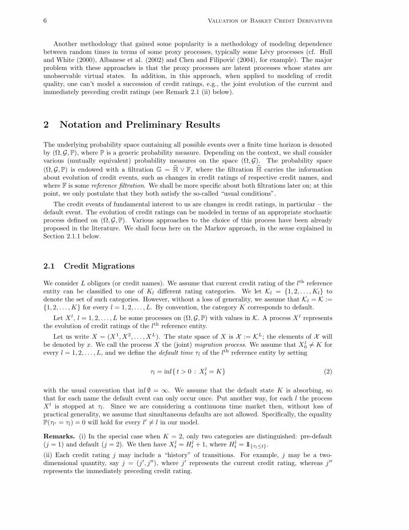
Another methodology that gained some popularity is a methodology of modeling dependencebetween random times in terms of some proxy processes, typically some Levy processes (cf. Hulland White (2000), Albanese et al. (2002) and Chen and Filipovic (2004), for example). The majorproblem with these approaches is that the proxy processes are latent processes whose states areunobservable virtual states. In addition, in this approach, when applied to modeling of creditquality, one can’t model a succession of credit ratings, e.g., the joint evolution of the current andimmediately preceding credit ratings (see Remark 2.1 (ii) below).
2 Notation and Preliminary Results
The underlying probability space containing all possible events over a finite time horizon is denotedby (Ω,G, P), where P is a generic probability measure. Depending on the context, we shall considervarious (mutually equivalent) probability measures on the space (Ω,G). The probability space
(Ω,G, P) is endowed with a filtration G = H ∨ F, where the filtration H carries the informationabout evolution of credit events, such as changes in credit ratings of respective credit names, andwhere F is some reference filtration. We shall be more specific about both filtrations later on; at thispoint, we only postulate that they both satisfy the so-called “usual conditions”.
The credit events of fundamental interest to us are changes in credit ratings, in particular – thedefault event. The evolution of credit ratings can be modeled in terms of an appropriate stochasticprocess defined on (Ω,G, P). Various approaches to the choice of this process have been alreadyproposed in the literature. We shall focus here on the Markov approach, in the sense explained inSection 2.1.1 below.
2.1 Credit Migrations
We consider L obligors (or credit names). We assume that current credit rating of the lth referenceentity can be classified to one of Kl different rating categories. We let Kl = 1, 2, . . . ,Kl todenote the set of such categories. However, without a loss of generality, we assume that Kl = K :=1, 2, . . . ,K for every l = 1, 2, . . . , L. By convention, the category K corresponds to default.
Let X l, l = 1, 2, . . . , L be some processes on (Ω,G, P) with values in K. A process X l representsthe evolution of credit ratings of the lth reference entity.
Let us write X = (X1, X2, . . . , XL). The state space of X is X := KL; the elements of X willbe denoted by x. We call the process X the (joint) migration process. We assume that X l
0 6= K forevery l = 1, 2, . . . , L, and we define the default time τl of the lth reference entity by setting
τl = inf t > 0 : X lt = K (2)
with the usual convention that inf ∅ = ∞. We assume that the default state K is absorbing, sothat for each name the default event can only occur once. Put another way, for each l the processX l is stopped at τl. Since we are considering a continuous time market then, without loss ofpractical generality, we assume that simultaneous defaults are not allowed. Specifically, the equalityP(τl′ = τl) = 0 will hold for every l′ 6= l in our model.
Remarks. (i) In the special case when K = 2, only two categories are distinguished: pre-default(j = 1) and default (j = 2). We then have X l
t = H lt + 1, where H l
t = 11τl≤t.
(ii) Each credit rating j may include a “history” of transitions. For example, j may be a two-dimensional quantity, say j = (j ′, j′′), where j′ represents the current credit rating, whereas j ′′
represents the immediately preceding credit rating.

T.R. Bielecki, M. Jeanblanc and M. Rutkowski 7
2.1.1 Markovian Set-up
From now on, we set H = FX , so that the filtration H is the natural filtration of the process X.Arguably, the most convenient set-up to work with is the one where the reference filtration F is thefiltration FY generated by relevant (vector) factor process, say Y , and where the process (X,Y ) is
jointly Markov under P with respect to its natural filtration G = FX ∨FY = H∨F, so that we have,for every 0 ≤ t ≤ s, x ∈ X and any set Y from the state space of Y ,
P(Xs = x, Ys ∈ Y | Gt) = P(Xs = x, Ys ∈ Y |Xt, Yt). (3)
This is the general framework adopted in the present paper. A specific Markov market model willbe introduced in Section 3 below.
Of primary importance in this paper will be the kth default time for an arbitrary k = 1, 2, . . . , L.Let τ (1) < τ (2) < · · · < τ (L) be the ordering (for each ω) of the default times τ1, τ2, . . . , τL. Bydefinition, the kth default time is τ (k).
It will be convenient to represent some probabilities associated with the kth default time in termsof the cumulative default process H, defined as the increasing process
Ht =
L∑
l=1
H lt ,
where H lt = 11Xl
t=K = 11τl≤t for every t ∈ R+. Evidently H ⊆ H, where H is the filtrationgenerated by the cumulative default process H. It is obvious that the process S := (H,X, Y ) hasthe Markov property under P with respect to the filtration G. Also, it is useful to observe thatwe have τ (1) > t = Ht = 0, τ (k) ≤ t = Ht ≥ k and τ (k) = τl = Hτl
= k for everyl, k = 1, 2, . . . , L.
2.2 Conditional Expectations
Although we shall later focus on a Markovian set-up, in the sense of equality (3), we shall firstderive some preliminary results in a more general set-up. To this end, it will be convenient to usethe notation FX,t = σ(Xs; s ≥ t) and FY,t = σ(Ys; s ≥ t) for the information generated by theprocesses X and Y after time t. We postulate that for any random variable Z ∈ FX,t ∨FY
∞ and anybounded measurable function g, it holds that
EP(g(Z) | Gt) = EP(g(Z) |σ(Xt) ∨ FYt ). (4)
This implies, in particular, that the migration process X is conditionally Markov with regard to thereference filtration FY , that is, for every 0 ≤ t ≤ s and x ∈ X ,
P(Xs = x | Gt) = P(Xs = x |σ(Xt) ∨ FYt ). (5)
Note that the Markov condition (3) is stronger than condition (4). We assume from now on thatt ≥ 0 and x ∈ X are such that px(t) := P(Xt = x | FY
t ) > 0. We begin the analysis of conditionalexpectations with the following lemma.
Lemma 2.1 Let k ∈ 1, 2, . . . , L, x ∈ X , and let Z ∈ FX,t ∨FY∞ be an integrable random variable.
Then we have, for every 0 ≤ t ≤ s,
11Xt=x EP(11Hs<kZ | Gt) = 11Ht<k, Xt=x
EP(11Hs<k, Xt=xZ | FYt )
px(t). (6)
Consequently,
EP(11Hs<kZ | Gt) = 11Ht<k
∑
x∈X
11Xt=x
EP(11Hs<k, Xt=xZ | FYt )
px(t). (7)
8 Valuation of Basket Credit Derivatives
Proof. Let At be an arbitrary event from Gt. We need to check that
EP
(11At
11Xt=x11Hs<kZ)
= EP
(11At
11Ht<k, Xt=x
EP(11Hs<k, Xt=xZ | FYt )
px(t)
).
Since Hs < k ⊂ Ht < k and the random variable Z := 11Hs<k, Xt=xZ belongs to FX,t ∨ FY∞,
the left-hand side is equal to
EP
(EP(11At
11Ht<k, Xt=x11Hs<kZ | Gt))
= EP
(11At
11Ht<k, Xt=x EP(11Hs<k, Xt=xZ | Gt))
= EP
(11At
11Ht<k, Xt=x EP(11Hs<k, Xt=xZ |σ(Xt) ∨ FYt ))
= EP
(11At
11Ht<k, Xt=x
EP(11Hs<k, Xt=xZ | FYt )
px(t)
),
where the second equality is a consequence of (4), and the last one follows from the equality
11Xt=x EP(Z |σ(Xt) ∨ FYt ) = 11Xt=x
EP(11Xt=xZ | FYt )
P(Xt = x | FYt )
,
which is valid for any integrable random variable Z. Equality (7) is an immediate consequence of(6). ¤
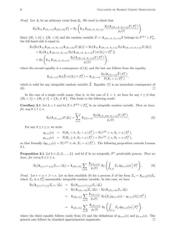
In the case of a single credit name, that is, in the case of L = 1, we have for any t ≥ 0 thatHt < 1 = Ht 6= 1 = Xt 6= K. This leads to the following result.
Corollary 2.1 Let L = 1 and let Z ∈ FX,t ∨ FY∞ be an integrable random variable. Then we have,
for any 0 ≤ t ≤ s,
EP(11Xs6=KZ | Gt) =
K−1∑
x=1
11Xt=x
EP(11Xs 6=K, Xt=xZ | FYt )
px(t). (8)
For any 0 ≤ t ≤ s, we write
qk,x;t(s) = P(Hs < k,Xt = x | FYt ) = P(τ (k) > s,Xt = x | FY
t ),
pk,x;t(s) = P(Hs ≥ k,Xt = x | FYt ) = P(τ (k) ≤ s,Xt = x | FY
t ),
so that formally dpk,x;t(s) = P(τ (k) ∈ ds,Xt = x | FYt ). The following proposition extends Lemma
2.1.
Proposition 2.1 Let k ∈ 1, 2, . . . , L and let Z be an integrable, FY -predictable process. Then wehave, for every 0 ≤ t ≤ s,
EP(11t<τ (k)≤sZτ (k) | Gt) = 11Ht<k
∑
x∈X
11Xt=x
px(t)EP
(∫
]t,s]
Zu dpk,x;t(u)∣∣∣FY
t
). (9)
Proof. Let t < α < β < s. Let us first establish (9) for a process Z of the form Zu = 11]α,β](u)Zα
where Zα is a FYα -measurable, integrable random variable. In this case, we have
EP(11t<τ (k)≤sZτ (k) | Gt) = EP(11α<τ (k)≤βZα | Gt)
= EP(11Hα<kZα | Gt) − EP(11Hβ<kZα | Gt)
= 11Ht<k
∑
x∈X
11Xt=x
px(t)EP
(Zα[qk,x,t(α) − qk,x,t(β)] | FY
t
)
= 11Ht<k
∑
x∈X
11Xt=x
px(t)EP
(∫
]t,s]
Zu dpk,x;t(u)∣∣∣FY
t
),
where the third equality follows easily from (7) and the definitions of qk,x;t(s) and pk,x;t(s). Thegeneral case follows by standard approximation arguments. ¤
T.R. Bielecki, M. Jeanblanc and M. Rutkowski 9
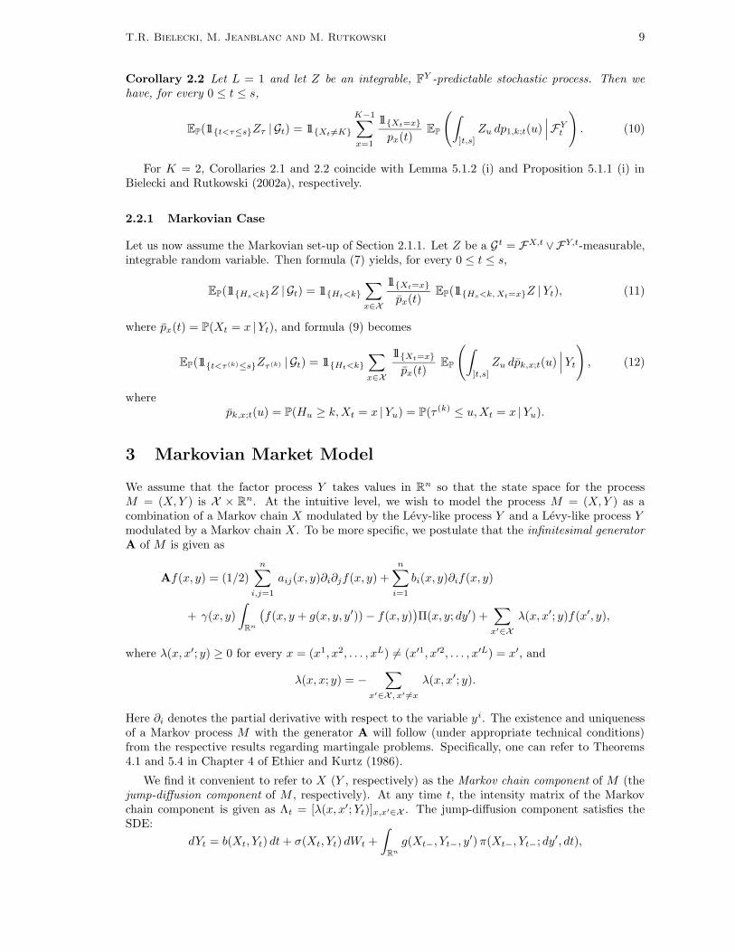
Corollary 2.2 Let L = 1 and let Z be an integrable, FY -predictable stochastic process. Then wehave, for every 0 ≤ t ≤ s,
EP(11t<τ≤sZτ | Gt) = 11Xt 6=K
K−1∑
x=1
11Xt=x
px(t)EP
(∫
]t,s]
Zu dp1,k;t(u)∣∣∣FY
t
). (10)
For K = 2, Corollaries 2.1 and 2.2 coincide with Lemma 5.1.2 (i) and Proposition 5.1.1 (i) inBielecki and Rutkowski (2002a), respectively.
2.2.1 Markovian Case
Let us now assume the Markovian set-up of Section 2.1.1. Let Z be a Gt = FX,t ∨FY,t-measurable,integrable random variable. Then formula (7) yields, for every 0 ≤ t ≤ s,
EP(11Hs<kZ | Gt) = 11Ht<k
∑
x∈X
11Xt=x
px(t)EP(11Hs<k, Xt=xZ |Yt), (11)
where px(t) = P(Xt = x |Yt), and formula (9) becomes
EP(11t<τ (k)≤sZτ (k) | Gt) = 11Ht<k
∑
x∈X
11Xt=x
px(t)EP
(∫
]t,s]
Zu dpk,x;t(u)∣∣∣Yt
), (12)
wherepk,x;t(u) = P(Hu ≥ k,Xt = x |Yu) = P(τ (k) ≤ u,Xt = x |Yu).
3 Markovian Market Model
We assume that the factor process Y takes values in Rn so that the state space for the processM = (X,Y ) is X × Rn. At the intuitive level, we wish to model the process M = (X,Y ) as acombination of a Markov chain X modulated by the Levy-like process Y and a Levy-like process Ymodulated by a Markov chain X. To be more specific, we postulate that the infinitesimal generatorA of M is given as
Af(x, y) = (1/2)
n∑
i,j=1
aij(x, y)∂i∂jf(x, y) +
n∑
i=1
bi(x, y)∂if(x, y)
+ γ(x, y)
∫
Rn
(f(x, y + g(x, y, y′)) − f(x, y)
)Π(x, y; dy′) +
∑
x′∈X
λ(x, x′; y)f(x′, y),
where λ(x, x′; y) ≥ 0 for every x = (x1, x2, . . . , xL) 6= (x′1, x′2, . . . , x′L) = x′, and
λ(x, x; y) = −∑
x′∈X , x′ 6=x
λ(x, x′; y).
Here ∂i denotes the partial derivative with respect to the variable yi. The existence and uniquenessof a Markov process M with the generator A will follow (under appropriate technical conditions)from the respective results regarding martingale problems. Specifically, one can refer to Theorems4.1 and 5.4 in Chapter 4 of Ethier and Kurtz (1986).
We find it convenient to refer to X (Y , respectively) as the Markov chain component of M (thejump-diffusion component of M , respectively). At any time t, the intensity matrix of the Markovchain component is given as Λt = [λ(x, x′;Yt)]x,x′∈X . The jump-diffusion component satisfies theSDE:
dYt = b(Xt, Yt) dt + σ(Xt, Yt) dWt +
∫
Rn
g(Xt−, Yt−, y′)π(Xt−, Yt−; dy′, dt),
10 Valuation of Basket Credit Derivatives
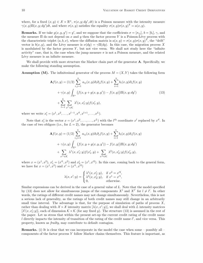
where, for a fixed (x, y) ∈ X × Rn, π(x, y; dy′, dt) is a Poisson measure with the intensity measureγ(x, y)Π(x, y; dy′)dt, and where σ(x, y) satisfies the equality σ(x, y)σ(x, y)T = a(x, y).
Remarks. If we take g(x, y, y′) = y′, and we suppose that the coefficients σ = [σij ], b = [bi], γ, andthe measure Π do not depend on x and y then the factor process Y is a Poisson-Levy process withthe characteristic triplet (a, b, ν), where the diffusion matrix is a(x, y) = σ(x, y)σ(x, y)T, the “drift”vector is b(x, y), and the Levy measure is ν(dy) = γΠ(dy). In this case, the migration process Xis modulated by the factor process Y , but not vice versa. We shall not study here the “infiniteactivity” case, that is, the case when the jump measure π is not a Poisson measure, and the relatedLevy measure is an infinite measure.
We shall provide with more structure the Markov chain part of the generator A. Specifically, wemake the following standing assumption.
Asumption (M). The infinitesimal generator of the process M = (X,Y ) takes the following form
Af(x, y) = (1/2)
n∑
i,j=1
aij(x, y)∂i∂jf(x, y) +
n∑
i=1
bi(x, y)∂if(x, y)
+ γ(x, y)
∫
Rn
(f(x, y + g(x, y, y′)) − f(x, y)
)Π(x, y; dy′) (13)
+
L∑
l=1
∑
xl′∈K
λl(x, x′l; y)f(x′
l, y),
where we write x′l = (x1, x2, . . . , xl−1, x′l, xl+1, . . . , xL).
Note that x′l is the vector x = (x1, x2, . . . , . . . , xL) with the lth coordinate xl replaced by x′l. In
the case of two obligors (i.e., for L = 2), the generator becomes
Af(x, y) = (1/2)
n∑
i,j=1
aij(x, y)∂i∂jf(x, y) +
n∑
i=1
bi(x, y)∂if(x, y)
+ γ(x, y)
∫
Rn
(f(x, y + g(x, y, y′)) − f(x, y)
)Π(x, y; dy′)
+∑
x′1∈K
λ1(x, x′1; y)f(x′
1, y) +∑
x′2∈K
λ2(x, x′2; y)f(x′
2, y),
where x = (x1, x2), x′1 = (x′1, x2) and x′
2 = (x1, x′2). In this case, coming back to the general form,we have for x = (x1, x2) and x′ = (x′1, x′2)
λ(x, x′; y) =
λ1(x, x′1; y), if x2 = x′2,
λ2(x, x′2; y), if x1 = x′1,
0, otherwise.
Similar expressions can be derived in the case of a general value of L. Note that the model specifiedby (13) does not allow for simultaneous jumps of the components X l and X l′ for l 6= l′. In otherwords, the ratings of different credit names may not change simultaneously. Nevertheless, this is nota serious lack of generality, as the ratings of both credit names may still change in an arbitrarilysmall time interval. The advantage is that, for the purpose of simulation of paths of process X,rather than dealing with X ×X intensity matrix [λ(x, x′; y)], we shall deal with L intensity matrices[λl(x, x′
l; y)], each of dimension K×K (for any fixed y). The structure (13) is assumed in the rest ofthe paper. Let us stress that within the present set-up the current credit rating of the credit namel directly impacts the intensity of transition of the rating of the credit name l′, and vice versa. Thisproperty, known as frailty, may contribute to default contagion.
Remarks. (i) It is clear that we can incorporate in the model the case when some – possibly all –components of the factor process Y follow Markov chains themselves. This feature is important, as
T.R. Bielecki, M. Jeanblanc and M. Rutkowski 11
factors such as economic cycles may be modeled as Markov chains. It is known that default ratesare strongly related to business cycles.
(ii) Some of the factors Y 1, Y 2, . . . , Y d may represent cumulative duration of visits of rating processes
X l in respective rating states. For example, we may set Y 1t =
∫ t
011X1
s =1 ds. In this case, we haveb1(x, y) = 11x1=1(x), and the corresponding components of coefficients σ and g equal zero.
(iii) In the area of structural arbitrage, so called credit–to–equity (C2E) models and/or equity–to–credit (E2C) models are studied. Our market model nests both types of interactions, that is C2Eand E2C. For example, if one of the factors is the price process of the equity issued by a credit name,and if credit migration intensities depend on this factor (implicitly or explicitly) then we have a E2Ctype interaction. On the other hand, if credit ratings of a given obligor impact the equity dynamics(of this obligor and/or some other obligors), then we deal with a C2E type interaction.
As already mentioned, S = (H,X, Y ) is a Markov process on the state space 0, 1, . . . , L×X ×Rd with respect to its natural filtration. Given the form of the generator of the process (X,Y ),we can easily describe the generator of the process (H,X, Y ). It is enough to observe that thetransition intensity at time t of the component H from the state Ht to the state Ht + 1 is equal
to∑L
l=1 λl(Xt,K;X(l)t , Yt), provided that Ht < L (otherwise, the transition intensity equals zero),
where we write X(l)t = (X1
t , . . . , X l−1t , X l+1
t , . . . , XLt ) and we set λl(xl, x′l;x(l), y) = λl(x, x′
l; y).
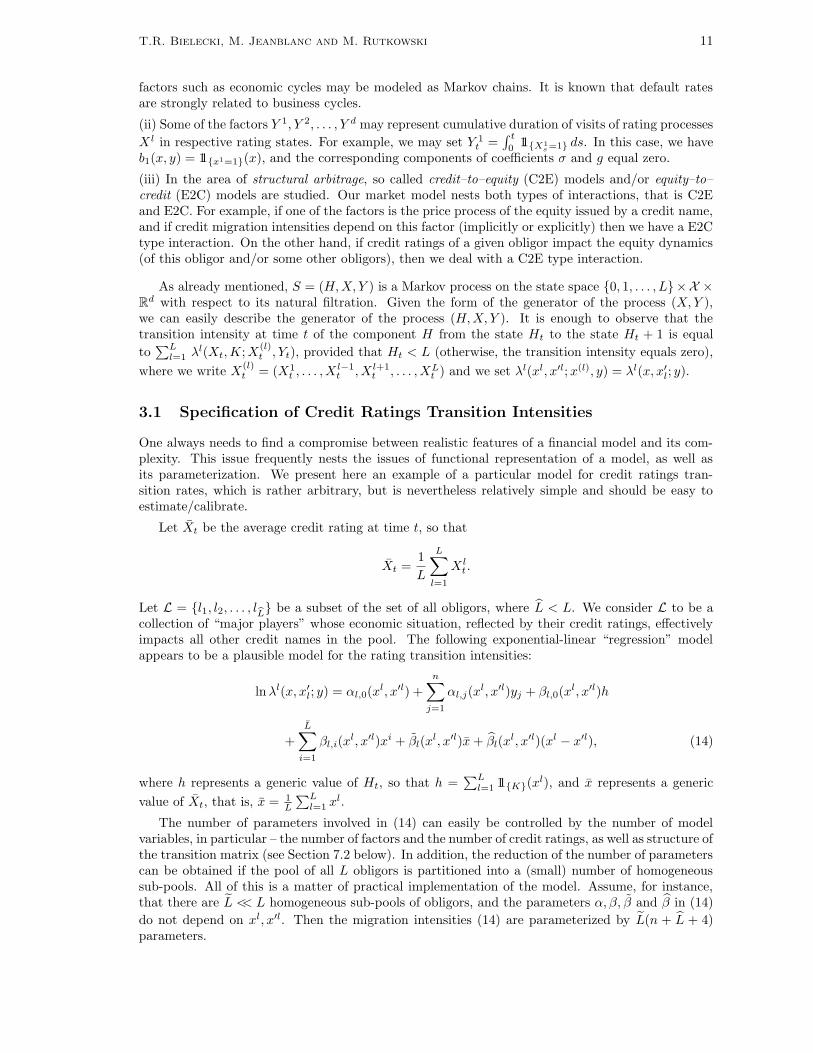
3.1 Specification of Credit Ratings Transition Intensities
One always needs to find a compromise between realistic features of a financial model and its com-plexity. This issue frequently nests the issues of functional representation of a model, as well asits parameterization. We present here an example of a particular model for credit ratings tran-sition rates, which is rather arbitrary, but is nevertheless relatively simple and should be easy toestimate/calibrate.
Let Xt be the average credit rating at time t, so that
Xt =1
L
L∑
l=1
X lt .
Let L = l1, l2, . . . , lbL be a subset of the set of all obligors, where L < L. We consider L to be a
collection of “major players” whose economic situation, reflected by their credit ratings, effectivelyimpacts all other credit names in the pool. The following exponential-linear “regression” modelappears to be a plausible model for the rating transition intensities:
ln λl(x, x′l; y) = αl,0(x
l, x′l) +n∑
j=1
αl,j(xl, x′l)yj + βl,0(x
l, x′l)h
+
L∑
i=1
βl,i(xl, x′l)xi + βl(x
l, x′l)x + βl(xl, x′l)(xl − x′l), (14)
where h represents a generic value of Ht, so that h =∑L
l=1 11K(xl), and x represents a generic
value of Xt, that is, x = 1L
∑Ll=1 xl.
The number of parameters involved in (14) can easily be controlled by the number of modelvariables, in particular – the number of factors and the number of credit ratings, as well as structure ofthe transition matrix (see Section 7.2 below). In addition, the reduction of the number of parameterscan be obtained if the pool of all L obligors is partitioned into a (small) number of homogeneoussub-pools. All of this is a matter of practical implementation of the model. Assume, for instance,that there are L << L homogeneous sub-pools of obligors, and the parameters α, β, β and β in (14)
do not depend on xl, x′l. Then the migration intensities (14) are parameterized by L(n + L + 4)parameters.

12 Valuation of Basket Credit Derivatives
3.2 Conditionally Independent Migrations
Suppose that the intensities λl(x, x′l; y) do not depend on x(l) = (x1, x2, . . . , xl−1, xl+1, . . . , xL) for
every l = 1, 2, . . . , L. In addition, assume that the dynamics of the factor process Y do not dependon the the migration process X. It turns out that in this case, given the structure of our generator asin (13), the migration processes X l, l = 1, 2, . . . , L, are conditionally independent given the samplepath of the process Y .
We shall illustrate this point in the case of only two credit names in the pool (i.e., for L = 2) andassuming that there is no factor process, so that conditional independence really means independencebetween migration processes X1 and X2. For this, suppose that X1 and X2 are independent Markovchains, each taking values in the state space K, with infinitesimal generator matrices Λ1 and Λ2,respectively. It is clear that the joint process X = (X1, X2) is a Markov chain on K × K. An easycalculation reveals that the infinitesimal generator of the process X is given as
Λ = Λ1 ⊗ IdK + IdK ⊗ Λ2,
where IdK is the identity matrix of order K and ⊗ denotes the matrix tensor product. This agreeswith the structure (13) in the present case.
4 Changes of Measures and Markovian Numeraires
In financial applications, one frequently deals with various absolutely continuous probability mea-sures. In order to exploit – for pricing applications – the Markovian structure of the market modelintroduced above, we need that the model is Markovian under a particular pricing measure corre-sponding to some particular numeraire process β that is convenient to use for some reasons. Themodel does not have to be Markovian under some other equivalent probability measures, such asthe statistical probability, say Q, or the spot martingale measure, say Q∗. Nevertheless, it maybe sometimes desirable that the Markovian structure of the market model is preserved under anequivalent change of a probability measure, for instance, when we change a numeraire from β to β ′.In this section, we shall provide some discussion of the issue of preservation of the Markov propertyof the process M .
Let T ∗ > 0 be a fixed horizon date, and let η be a strictly positive, GT∗ -measurable randomvariable such that EPη = 1. We define an equivalent probability measure Pη on (Ω,GT∗) by theequality
dPη
dP= η, P-a.s.
4.1 Markovian Change of a Probability Measure
We place ourselves in the set-up of Section 2.1.1, and we follow Palmowski and Rolski (2002) inthe presentation below. The standing assumption is that the process M = (X,Y ) has the Markovproperty under P with respect to the filtration G. Let (A,D(A)) be the extended generator of M .This means that the process
Mft = f(Mt) −
∫ t
0
Af(Ms) ds (15)
is a local G-martingale for any function f in D(A).
For any strictly positive function h ∈ D(A), we define an auxiliary process ηh by setting
ηht =
h(Mt)
h(M0)exp
(−
∫ t
0
(Ah)(Ms)
h(Ms)ds
), t ∈ [0, T ∗]. (16)
Any function h for which the process ηh is a martingale is called a good function for A. Observethat for any such function h, the equality EP(ηh
t ) = 1 holds for every t ∈ [0, T ∗]. Note also that any

T.R. Bielecki, M. Jeanblanc and M. Rutkowski 13
constant function h is a good function for A; in this case we have, of course, that ηh ≡ 1. The nextlemma follows from results of Palmowski and Rolski (2002) (see Lemma 3.1 therein).
Lemma 4.1 Let h be a good function for A. Then the process ηh is given as Doleans exponentialmartingale
ηht = Et(N
h),
where the local martingale Nh is given as
Nht =
∫ t
0
κhs− dMh
s
with κht = 1/h(Mt). In other words, the process ηh satisfies the SDE
dηht = ηh
t−κht− dMh
t , ηh0 = 1. (17)
Proof. An application of Ito’s formula yields
dηht =
1
h(M0)exp
(−
∫ t
0
(Ah)(Ms)
h(Ms)ds
)dMh
t ,
where the local martingale Mh is given by (15). This proves formula (17). ¤
For any good function h for A, we define an equivalent probability measure Ph on (Ω,GT∗) bysetting
dPh
dP= ηh
T∗ , P-a.s. (18)
From Kunita and Watanabe (1963), we deduce that the process M preserves its Markov propertywith respect to the filtration G when the probability measure P is replaced by Ph. In order to findthe extended generator of M under Ph, we set
Ahf =1
h[A(fh) − fA(h)] ,
and we define the following two sets:
DhA
=
f ∈ D(A) : fh ∈ D(A) and
∫ T∗
0
|Ahf(Ms)| ds < ∞, Ph-a.s.
and
Dh−1
Ah =
f ∈ D(Ah) : fh−1 ∈ D(Ah) and
∫ T∗
0
|Af(Ms)| ds < ∞, P-a.s.
.
Then the following result holds (see Theorem 4.2 in Palmowski and Rolski (2002)).
Theorem 4.1 Suppose that DhA
= D(A) and Dh−1
Ah = D(Ah). Then the process M is Markovianunder Ph with the extended generator Ah and D(Ah) = D(A).
We now apply the above theorem to our model. The domain of D(A) contains all functionsf(x, y) with compact support that are twice continuously differentiable with respect to y. Let h bea good function. Under mild assumptions on the coefficients of A, the assumptions of Theorem 4.1are satisfied. It follows that the generator of M under Ph is given as
Ahf(x, y) = (1/2)
n∑
i,j=1
aij(x, y)∂i∂jf(x, y) +
n∑
i=1
bhi (x, y)∂if(x, y)
+ γ(x, y)
∫
Rn
(f(x, y + g(x, y, y′)) − f(x, y)) Πh(x, y; dy′) +∑
x′∈X
λh(x, x′; y)f(x′, y),

14 Valuation of Basket Credit Derivatives
where
bhi (x, y) = bi(x, y) +
1
h(x, y)
n∑
i,j=1
aij(x, y)∂jh(x, y),
Πh(x, y; dy′) =h(x, y + g(x, y, y′))
h(x, y)Π(x, y; dy′), (19)
λh(x, x′; y) = λ(x, x′; y)h(x′, y)
h(x, y), x 6= x′, λh(x, x; y) = −
∑
x′ 6=x
λh(x, x′; y).
Before we proceed to the issue of valuation of credit derivatives, we state the following useful result,whose easy proof is omitted.
Lemma 4.2 Let h and h′ be two good functions for A. Then φ(h, h′) := h′/h is a good function forAh. Moreover, we have that
dPh′
dPh= η
φ(h,h′)T∗ , Ph-a.s. (20)
where the process ηφ(h,h′) is defined in analogy to (16) with A replaced with Ah.
4.2 Markovian Numeraires and Valuation Measures
Let us first consider a general set-up. We use here the notation and terminology of Jamshidian(2004). We fix the horizon date T ∗, and we assume that G = GT∗ . Let us fix some (G-adapted)deflator process ξ, that is, a strictly positive, integrable semimartingale, with ξ0 = 1. Any G-measurable random variable C such that ξT∗C is integrable under P is called a claim. The priceprocess Ct, t ∈ [0, T ∗], of a claim C is formally defined as
Ct = ξ−1t EP(ξT∗C | Gt),
so that, in particular, CT∗ = C. It is implicitly assumed here that the information carried by thefiltration G is available to all trading agents.
Suppose that we are interested in providing valuation formulae for some financial products, andsuppose that we find it convenient to use a particular numeraire (that is, a strictly positive claim),denoted by β. Let Pβ be the corresponding valuation measure, defined on (Ω,G) as
dPβ
dP=
ξT∗β
β0=
ξT∗βT∗
β0, P-a.s. (21)
From the abstract Bayes rule, it follows that the price process C can be expressed as follows:
Ct = βt EPβ (β−1T∗ C | Gt).
As before, we assume that our market model M is Markovian under P, where P might bethe statistical probability measure Q, the spot martingale measure Q∗, or some other martingalemeasure. We want the process M to remain a time-homogeneous Markov process under Pβ .
Definition 4.1 A valuation measure Pβ is said to be a Markovian if the process M remains a time-homogeneous Markov process under Pβ . Any numeraire process β such that the valuation measurePβ is Markovian is called a Markovian numeraire.
In view of results of Section 4.1, for a valuation measure Pβ to be Markovian, it suffices that the
Radon-Nikodym derivative process ηβt = dP
β
dP
∣∣Gt
satisfies
ηβt =
hβ(Mt)
hβ(M0)exp
(−
∫ t
0
(Ahβ)(Ms)
hβ(Ms)ds
), t ∈ [0, T ∗],

T.R. Bielecki, M. Jeanblanc and M. Rutkowski 15
for some good function hβ for A. The corresponding deflator process is then given as ξβt = β0β
−1t ηβ
t ,that is, for any claim C we have that
Ct = βt EPβ (β−1T∗ C | Gt) = (ξβ
t )−1 EP(ξβT∗C | Gt).
If β and β′ are two such numeraires, and hβ and hβ′
are the corresponding good functions then, inview of Lemma 4.2, we have
dPβ′
dPβ= η
φ(hβ ,hβ′)
T∗ , Pβ-a.s. (22)
An interesting question arises: under what conditions on ξ and β the probability measure Pβ isa Markovian valuation measure? In order to partially address this question, we shall consider thecase where the valuation measure Pβ is a Markovian for any constant numeraire β, that is, for anyβ ≡ const > 0.
Proposition 4.1 Assume that the deflator process satisfies ξ = ηh for some good function h for A.Then the following statements are true:(i) for any constant numeraire β, the valuation measure Pβ is Markovian,(ii) if a numeraire β is such that β = β0η
χT∗/ηh
T∗ for some good function χ for A, then the valuationmeasure Pβ is Markovian,
(iii) if numeraires β and β′ are such that β = β0ηχT∗/ηh
T∗ and β′ = β′0η
χ′
T∗/ηhT∗ for some good functions
χ and χ′ for A, then
dPβ′
dPβ=
β′/β′0
β/β0=
ηχ′
T∗
ηχT∗
, Pξ,β′
-a.s. (23)
Proof. Let ξ = ηh for some good function h, where ηh is given by (16). Then for any constantnumeraire β we get Pβ = Ph and thus, by results of Kunita and Watanabe (1963), the process M isMarkovian under the valuation measure Pβ . This proves part (i). To establish the second part, itsuffices to note that
dPβ
dP=
ξT∗β
β0= ηχ
T∗ ,
and to use again the result of Kunita and Watanabe (1963). Formula (23) follows easily from (21)(it can also be seen as a special case of (22)). This completes the proof. ¤
4.3 Examples of Markov Market Models
We shall now present three pertinent examples of Markov market models. We assume here that anumaraire β is given; the choice of β depends on the problem at hand.
4.3.1 Markov Chain Migration Process
We assume here that there is no factor process Y . Thus, we only deal with a single migration processX. In this case, an attractive and efficient way to model credit migrations is to postulate that Xis a birth-and-death process with absorption at state K. In this case, the intensity matrix Λ is tri-diagonal. To simplify the notation, we shall write pt(k, k′) = Pβ(Xs+t = k′ |Xs = k). The transitionprobabilities pt(k, k′) satisfy the following system of ODEs, for t ≥ 0 and k′ ∈ 1, 2, . . . ,K,
dpt(1, k′)
dt= −λ(1, 2)pt(1, k
′) + λ(1, 2)pt(2, k′),
dpt(k, k′)
dt= λ(k, k − 1)pt(k − 1, k′) − (λ(k, k − 1) + λ(k, k + 1))pt(k, k′) + λ(k, k + 1)pt(k + 1, k′)
for k = 2, 3, . . . ,K − 1, anddpt(K, k′)
dt= 0,

16 Valuation of Basket Credit Derivatives
with initial conditions p0(k, k′) = 11k=k′. Once the transition intensities λ(k, k′) are specified, theabove system can be easily solved. Note, in particular, that pt(K, k′) = 0 for every t if k′ 6= K. Theadvantage of this representation is that the number of parameters can be kept small.
A slightly more flexible model is produced if we allow for jumps to the default state K from anyother state. In this case, the master ODEs take the following form, for t ≥ 0 and k′ ∈ 1, 2, . . . ,K,
dpt(1, k′)
dt= −(λ(1, 2) + λ(1,K))pt(1, k
′) + λ(1, 2)pt(2, k′) + λ(1,K)pt(K, k′),
dpt(k, k′)
dt= λ(k, k − 1)pt(k − 1, k′) − (λ(k, k − 1) + λ(k, k + 1) + λ(k,K))pt(k, k′)
+λ(k, k + 1)pt(k + 1, k′) + λ(k,K)pt(K, k′)
for k = 2, 3, . . . ,K − 1, anddpt(K, k′)
dt= 0,
with initial conditions p0(k, k′) = 11k=k′. Some authors model migrations of credit ratings usinga (proxy) diffusion, possibly with jumps to default. The birth-and-death process with jumps todefault furnishes a Markov chain counterpart of such proxy diffusion models. The nice feature of theMarkov chain model is that the credit ratings are (in principle) observable state variables – whereasin case of the proxy diffusion models they are not.
4.3.2 Diffusion-type Factor Process
We now add a factor process Y to the model. We postulate that the factor process is a diffusionprocess and that the generator of the process M = (X,Y ) takes the form
Af(x, y) = (1/2)
n∑
i,j=1
aij(x, y)∂i∂jf(x, y) +
n∑
i=1
bi(x, y)∂if(x, y)
+∑
x′∈K, x′ 6=x
λ(x, x′; y)(f(x′, y) − f(x, y)).
Let φ(t, x, y, x′, y′) be the transition probability of M . Formally,
φ(t, x, y, x′, y′) dy′ = Pβ(Xs+t = x′, Ys+t ∈ dy′ |Xs = x, Ys = y).
In order to determine the function φ, we need to study the following Kolmogorov equation
dv(s, x, y)
ds+ Av(s, x, y) = 0. (24)
For the generator A of the present form, equation (24) is commonly known as the reaction-diffusionequation. Existence and uniqueness of classical solutions for such equations were recently studied byBecherer and Schweizer (2003). It is worth mentioning that a reaction-diffusion equation is a specialcase of a more general integro-partial-differential equation (IPDE). In a future work, we shall dealwith issue of practical solving of equations of this kind.
4.3.3 CDS Spread Factor Model
Suppose now that the factor process Yt = κ(1)(t, TS , TM ) is the forward CDS spread (for thedefinition of κ(1)(t, TS , TM ), see Section 5.3 below), and that the generator for (X,Y ) is
Af(x, y) = (1/2)y2a(x)d2f(x, y)
dy2+
∑
x′∈K, x′ 6=x
λ(x, x′)(f(x′, y) − f(x, y)).

T.R. Bielecki, M. Jeanblanc and M. Rutkowski 17
Thus, the credit spread satisfies the following SDE
dκ(1)(t, TS , TM ) = κ(1)(t, TS , TM )σ(Xt) dWt
for some Brownian motion process W , where σ(x) =√
a(x). Note that in this example κ(1)(t, TS , TM )is a conditionally log-Gaussian process given a sample path of the migration process X, so that weare in the position to make use of Proposition 5.1 below.
5 Valuation of Single Name Credit Derivatives
We maintain the Markovian set-up, so that M = (X,Y ) follows a Markov process with respect to G
under P. In this section, we only consider one underlying credit name, that is, we set L = 1. Basketcredit derivatives will be studied in Section 6 below.
5.1 Survival Claims
Suppose that β is a Markovian numeraire, in the sense of Definition 4.1. Let us fix t ∈ [0, T ],and let us assume that a claim C and the random variable βt/βT∗ are measurable with respect to
Gt = FX,t ∨ FY,t. Then we deduce easily that Ct = Vξ,βt (C), where
Vξ,βt (C) = EPβ
(βtβ
−1T∗ C
∣∣Mt
).
A claim C such that C = 0 on the set τ ≤ T, so that
C = 11τ>TC = 11XT 6=KC = 11HT <1C,
is termed a T -survival claim. For a survival claim, a more explicit expression for the price can beestablished. Since most standard credit derivatives can be seen as survival claims, the followingsimple result will prove useful in what follows.
Lemma 5.1 Assume that a claim C and that the random variable βt/βT∗ are measurable withrespect to Gt. If C is a T -survival claim then we have
Ct = 11Xt 6=K Vξ,βt (C) =
K−1∑
x=1
11Xt=x
EPβ (11Xt=xβtβ−1T∗ C |Yt)
Pβ(Xt = x |Yt).
Proof. The first equality is clear. To derive the second equality above, it suffices to apply formula(11) with L = 1, s = T, k = 1 and Z = C. ¤
Remark. Assume that K = 2, so that only the pre-default state (x = 1) and the default state(x = 2) are recognized. Then we have, for any T -survival claim C,
Ct = 11Xt 6=2 Vξ,βt (C) =
11Xt=1Vξ,βt (C)
Pβ(Xt = 1 |Yt),
where V ξ,βt (C) = EPβ (βtβ
−1T∗ C |Yt). In the paper by Jamshidian (2004), the process V ξ,β
t (C) istermed the preprice of C.
5.2 Credit Default Swaps
The standing assumption is that β is a Markovian numeraire and βt/βs is Gt-measurable for anyt ≤ s. For simplicity, we shall discuss a vanilla credit default swap (CDS, for short) written ona corporate discount bond under the fractional recovery of par covenant. We suppose that thematurity of the reference bond is U , and the maturity of the swap is T < U .
18 Valuation of Basket Credit Derivatives
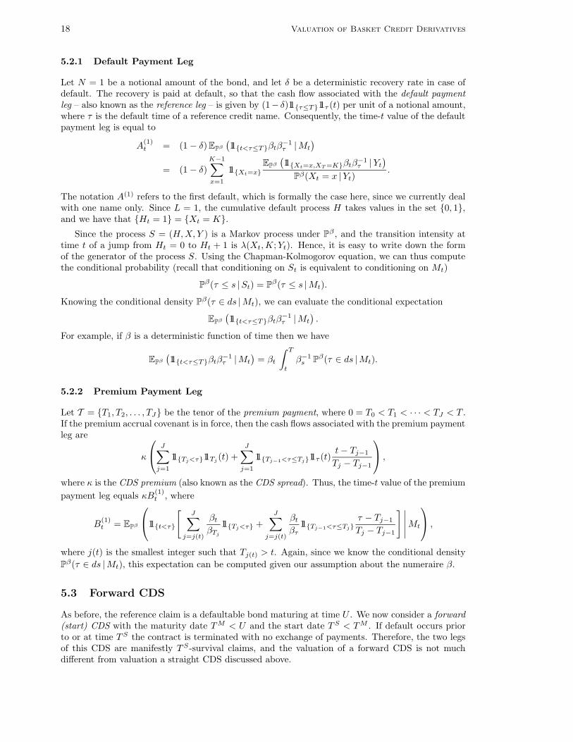
5.2.1 Default Payment Leg
Let N = 1 be a notional amount of the bond, and let δ be a deterministic recovery rate in case ofdefault. The recovery is paid at default, so that the cash flow associated with the default paymentleg – also known as the reference leg – is given by (1− δ)11τ≤T11τ (t) per unit of a notional amount,where τ is the default time of a reference credit name. Consequently, the time-t value of the defaultpayment leg is equal to
A(1)t = (1 − δ) EPβ
(11t<τ≤Tβtβ
−1τ |Mt
)
= (1 − δ)K−1∑
x=1
11Xt=x
EPβ
(11Xt=x,XT =Kβtβ
−1τ |Yt
)
Pβ(Xt = x |Yt).
The notation A(1) refers to the first default, which is formally the case here, since we currently dealwith one name only. Since L = 1, the cumulative default process H takes values in the set 0, 1,and we have that Ht = 1 = Xt = K.
Since the process S = (H,X, Y ) is a Markov process under Pβ , and the transition intensity attime t of a jump from Ht = 0 to Ht + 1 is λ(Xt,K;Yt). Hence, it is easy to write down the formof the generator of the process S. Using the Chapman-Kolmogorov equation, we can thus computethe conditional probability (recall that conditioning on St is equivalent to conditioning on Mt)
Pβ(τ ≤ s |St) = Pβ(τ ≤ s |Mt).
Knowing the conditional density Pβ(τ ∈ ds |Mt), we can evaluate the conditional expectation
EPβ
(11t<τ≤Tβtβ
−1τ |Mt
).
For example, if β is a deterministic function of time then we have
EPβ
(11t<τ≤Tβtβ
−1τ |Mt
)= βt
∫ T
t
β−1s Pβ(τ ∈ ds |Mt).
5.2.2 Premium Payment Leg
Let T = T1, T2, . . . , TJ be the tenor of the premium payment, where 0 = T0 < T1 < · · · < TJ < T .If the premium accrual covenant is in force, then the cash flows associated with the premium paymentleg are
κ
J∑
j=1
11Tj<τ11Tj(t) +
J∑
j=1
11Tj−1<τ≤Tj11τ (t)t − Tj−1
Tj − Tj−1
,
where κ is the CDS premium (also known as the CDS spread). Thus, the time-t value of the premium
payment leg equals κB(1)t , where
B(1)t = EPβ
11t<τ
[J∑
j=j(t)
βt
βTj
11Tj<τ +J∑
j=j(t)
βt
βτ
11Tj−1<τ≤Tjτ − Tj−1
Tj − Tj−1
] ∣∣∣∣∣Mt
,
where j(t) is the smallest integer such that Tj(t) > t. Again, since we know the conditional density
Pβ(τ ∈ ds |Mt), this expectation can be computed given our assumption about the numeraire β.
5.3 Forward CDS
As before, the reference claim is a defaultable bond maturing at time U . We now consider a forward(start) CDS with the maturity date T M < U and the start date T S < TM . If default occurs priorto or at time T S the contract is terminated with no exchange of payments. Therefore, the two legsof this CDS are manifestly T S-survival claims, and the valuation of a forward CDS is not muchdifferent from valuation a straight CDS discussed above.

T.R. Bielecki, M. Jeanblanc and M. Rutkowski 19
5.3.1 Default Payment Leg
As before, we let N = 1 be the notional amount of the bond, and we let δ be a deterministic recoveryrate in case of default. The recovery is paid at default, so that the cash flow associated with thedefault payment leg of the forward CDS can be represented as follows
(1 − δ)11T S<τ≤T M11τ (t).
For any t ≤ T S , the time-t value of the default payment leg is equal to
A(1),T S
t = (1 − δ) EPβ
(11T S<τ≤T Mβtβ
−1τ |Mt
).
As explained above, we can compute this conditional expectation. If β is a deterministic functionof time then simply
EPβ
(11T S<τ≤T Mβtβ
−1τ |Mt
)= βt
∫ T M
T S
β−1s Pβ(τ ∈ ds |Mt).
5.3.2 Premium Payment Leg
Let T = T1, T2, . . . , TJ be the tenor of premium payment, where T S < T1 < · · · < TJ < TM . Asbefore, we assume that the premium accrual covenant is in force, so that the cash flows associatedwith the premium payment leg are
κ
J∑
j=1
11Tj<τ11Tj(t) +
J∑
j=1
11Tj−1<τ≤Tj11τ (t)t − Tj−1
Tj − Tj−1
.
Thus, for any t ≤ T S the time-t value of the premium payment leg is κB(1),T S
t , where
B(1),T S
t = EPβ
11TS<τ
[J∑
j=1
βt
βTj
11Tj<τ +
J∑
j=1
βt
βτ
11Tj−1<τ≤Tjτ − Tj−1
Tj − Tj−1
] ∣∣∣∣∣Mt
.
Again, knowing the conditional density Pβ(τ ∈ ds |Mt), we can evaluate this conditional expectation.
5.4 CDS Swaptions
We consider a forward CDS swap starting at T S and maturing at T M > TS , as described in theprevious section. We shall now value the corresponding CDS swaption with expiry date T < T S .Let K be the strike CDS rate of the swaption. Then the swaption cash flow at expiry date T equals
(A
(1),T S
T − KB(1),T S
T
)+,
so that the price of the swaption equals, for any t ≤ T ,
EPβ
(βtβ
−1T
(A
(1),T S
T − KB(1),T S
T
)+ ∣∣∣Mt
)= EPβ
(βtβ
−1T B
(1),T S
T
(κ(1)(t, TS , TM ) − K
)+ ∣∣∣Mt
),
where κ(1)(t, TS , TM ) := A(1),T S
t /B(1),T S
t is the forward CDS rate. Note that the random variables
A(1),T S
t and B(1),T S
t are strictly positive on the set τ > T for t ≤ T < T S , so that κ(1)(t, TS , TM )enjoys the same property.
20 Valuation of Basket Credit Derivatives
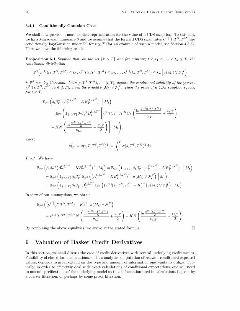
5.4.1 Conditionally Gaussian Case
We shall now provide a more explicit representation for the value of a CDS swaption. To this end,we fix a Markovian numeraire β and we assume that the forward CDS swap rates κ(1)(t, TS , TM ) areconditionally log-Gaussian under Pβ for t ≤ T (for an example of such a model, see Section 4.3.3).Then we have the following result.
Proposition 5.1 Suppose that, on the set τ > T and for arbitrary t < t1 < · · · < tn ≤ T , theconditional distribution
Pβ(κ(1)(t1, T
S , TM ) ≤ k1, κ(1)(t2, T
S , TM ) ≤ k2, . . . , κ(1)(tn, TS , TM ) ≤ kn
∣∣∣σ(Mt) ∨ FXT
)
is Pβ-a.s. log-Gaussian. Let σ(s, T S , TM ), s ∈ [t, T ], denote the conditional volatility of the processκ(1)(s, TS , TM ), s ∈ [t, T ], given the σ-field σ(Mt) ∨FX
T . Then the price of a CDS swaption equals,for t < T ,
EPβ
(βtβ
−1T
(A
(1),T S
T − KB(1),T S
T
)+ ∣∣∣Mt
)
= EPβ
(11τ>Tβtβ
−1T B
(1),T S
T
[κ(1)(t, TS , TM )N
(ln κ(1)(t,T S ,T M )
K
υt,T
+υt,T
2
)
− KN
(ln κ(1)(t,T S ,T M )
K
υt,T
−υt,T
2
)] ∣∣∣∣∣Mt
),
where
υ2t,T = υ(t, T, T S , TM )2 :=
∫ T
t
σ(s, T S , TM )2 ds.
Proof. We have
EPβ
(βtβ
−1T
(A
(1),T S
T − KB(1),T S
T
)+ ∣∣∣Mt
)= EPβ
(11τ>Tβtβ
−1T
(A
(1),T S
T − KB(1),T S
T
)+ ∣∣∣Mt
)
= EPβ
(11τ>Tβtβ
−1T EPβ
((A
(1),T S
T − KB(1),T S
T
)+|σ(Mt) ∨ FX
T
) ∣∣∣Mt
)
= EPβ
(11τ>Tβtβ
−1T B
(1),T S
T EPβ
((κ(1)(T, TS , TM ) − K
)+|σ(Mt) ∨ FX
T
) ∣∣∣Mt
).
In view of our assumptions, we obtain
EPβ
((κ(1)(T, TS , TM ) − K
)+ ∣∣∣σ(Mt) ∨ FXT
)
= κ(1)(t, TS , TM )N
(ln κ(1)(t,T S ,T M )
K
υt,T
+υt,T
2
)− KN
(ln κ(1)(t,T S ,T M )
K
υt,T
−υt,T
2
).
By combining the above equalities, we arrive at the stated formula. ¤
6 Valuation of Basket Credit Derivatives
In this section, we shall discuss the case of credit derivatives with several underlying credit names.Feasibility of closed-form calculations, such as analytic computation of relevant conditional expectedvalues, depends to great extend on the type and amount of information one wants to utilize. Typ-ically, in order to efficiently deal with exact calculations of conditional expectations, one will needto amend specifications of the underlying model so that information used in calculations is given bya coarser filtration, or perhaps by some proxy filtration.
T.R. Bielecki, M. Jeanblanc and M. Rutkowski 21
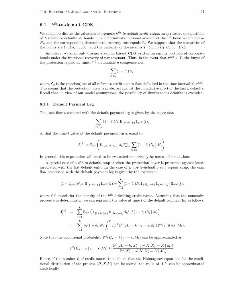
6.1 kth-to-default CDS
We shall now discuss the valuation of a generic kth-to-default credit default swap relative to a portfolioof L reference defaultable bonds. The deterministic notional amount of the ith bond is denoted asNi, and the corresponding deterministic recovery rate equals δi. We suppose that the maturities ofthe bonds are U1, U2, . . . , UL, and the maturity of the swap is T < min U1, U2, . . . , UL.
As before, we shall only discuss a vanilla basket CDS written on such a portfolio of corporatebonds under the fractional recovery of par covenant. Thus, in the event that τ (k) < T , the buyer ofthe protection is paid at time τ (k) a cumulative compensation
∑
i∈Lk
(1 − δi)Ni,
where Lk is the (random) set of all reference credit names that defaulted in the time interval ]0, τ (k)].This means that the protection buyer is protected against the cumulative effect of the first k defaults.Recall that, in view of our model assumptions, the possibility of simultaneous defaults is excluded.
6.1.1 Default Payment Leg
The cash flow associated with the default payment leg is given by the expression
∑
i∈Lk
(1 − δi)Ni11τ (k)≤T11τ (k)(t),
so that the time-t value of the default payment leg is equal to
A(k)t = EPβ
(11t<τ (k)≤Tβtβ
−1τ (k)
∑
i∈Lk
(1 − δi)Ni
∣∣∣Mt
).
In general, this expectation will need to be evaluated numerically by means of simulations.
A special case of a kth-to-default-swap is when the protection buyer is protected against lossesassociated with the last default only. In the case of a last-to-default credit default swap, the cashflow associated with the default payment leg is given by the expression
(1 − δι(k))Nι(k)11τ (k)≤T11τ (k)(t) =
L∑
i=1
(1 − δi)Ni11Hτi=k11τ (i)≤T11τ (i)(t),
where ι(k) stands for the identity of the kth defaulting credit name. Assuming that the numeraireprocess β is deterministic, we can represent the value at time t of the default payment leg as follows:
A(k)t =
L∑
i=1
EPβ
(11t<τi≤T11Hτi
=kβtβ−1τi
(1 − δi)Ni |Mt
)
=L∑
i=1
βt(1 − δi)Ni
∫ T
t
β−1s Pβ(Hs = k | τi = s,Mt) Pβ(τi ∈ ds |Mt).
Note that the conditional probability Pβ(Hs = k | τi = s,Mt) can be approximated as
Pβ(Hs = k | τi = s,Mt) ≈Pβ(Hs = k,Xi
s−ε 6= K,Xis = K |Mt)
Pβ(Xis−ε 6= K,Xi
s = K |Mt).
Hence, if the number L of credit names is small, so that the Kolmogorov equations for the condi-
tional distribution of the process (H,X, Y ) can be solved, the value of A(k)t can be approximated
analytically.
22 Valuation of Basket Credit Derivatives
6.1.2 Premium Payment Leg
Let T = T1, T2, . . . , TJ denote the tenor of the premium payment, where 0 = T0 < T1 < · · · <TJ < T . If the premium accrual covenant is in force, then the cash flows associated with the premiumpayment leg admit the following representation:
κ(k)
J∑
j=1
11Tj<τ (k)11Tj(t) +
J∑
j=1
11Tj−1<τ (k)≤Tj11τ (k)(t)t − Tj−1
Tj − Tj−1
,
where κ(k) is the CDS premium. Thus, the time-t value of the premium payment leg is κ(k)B(k)t ,
where
B(k)t = EPβ
11t<τ (k)
N∑
j=j(t)
βt
βTj
11Tj<τ (k)
∣∣∣∣∣Mt
+ EPβ
11t<τ (k)
J∑
j=j(t)
βt
βτ (k)
11Tj−1<τ (k)≤Tj
τ (k) − Tj−1
Tj − Tj−1
∣∣∣∣∣Mt
,
where j(t) is the smallest integer such that Tj(t) > t. Again, in general, the above conditionalexpectation will need to be approximated by simulation. And again, for a small portfolio size L,if either exact or numerical solution of relevant Kolmogorov equations can be derived, then ananalytical computation of the expectation can be done. This is left for a future study.
6.2 Forward kth-to-default CDS
Forward kth-to-default CDS is an analogous structure to the forward CDS. The notation used hereis consistent with the notation used previously in Sections 5.3 and 6.1.
6.2.1 Default Payment Leg
The cash flow associated with the default payment leg can be expressed as follows∑
i∈Lk
(1 − δi)Ni11T S<τ (k)≤T M11τ (k)(t).
Consequently, the time-t value of the default payment leg equals, for every t ≤ T S ,
A(k),T S
t = EPβ
(11T S<τ (k)≤T Mβtβ
−1τ (k)
∑
i∈Lk
(1 − δi)Ni
∣∣∣Mt
).
6.2.2 Premium Payment Leg
As before, let T = T1, T2, . . . , TJ be the tenor of a generic premium payment leg, where T S <T1 < · · · < TJ < TM . Under the premium accrual covenant, the cash flows associated with thepremium payment leg are
κ(k)
J∑
j=1
11Tj<τ (k)11Tj(t) +
J∑
j=1
11Tj−1<τ (k)≤Tj11τ (k)(t)t − Tj−1
Tj − Tj−1
,
where κ(k) is the CDS premium. Thus, the time-t value of the premium payment leg is κ(k)B(k),T S
t ,where
B(k),T S
t = EPβ
11t<τ (k)
[N∑
j=1
βt
βTj
11Tj<τ +
J∑
j=1
βt
βτ
11Tj−1<τ (k)≤Tj
τ − Tj−1
Tj − Tj−1
] ∣∣∣∣∣Mt
.
T.R. Bielecki, M. Jeanblanc and M. Rutkowski 23
7 Model Implementation
The last section is devoted to a brief discussion of issues related to the model implementation.
7.1 Curse of Dimensionality
When one deals with basket products involving multiple credit names, direct computations maynot be feasible. The cardinality of the state space K for the migration process X is equal to KL.Thus, for example, in case of K = 18 rating categories, as in Moody’s ratings,1 and in case of aportfolio of L = 100 credit names, the state space K has 18100 elements.2 If one aims at closed-form expressions for conditional expectations, but K is large, then it will typically be infeasible towork directly with information provided by the state vector (X,Y ) = (X1, X2, . . . , XL, Y ) and withthe corresponding generator A. A reduction in the amount of information that can be effectivelyused for analytical computations will be needed. Such reduction may be achieved by reducing thenumber of distinguished rating categories – this is typically done by considering only two categories:pre-default and default. However, this reduction may still not be sufficient enough, and furthersimplifying structural modifications to the model may need to be called for. Some types of additionalmodifications, such as homogeneous grouping of credit names and the mean-field interactions betweencredit names, are discussed in Frey and Backhaus (2004).3
7.2 Recursive Simulation Procedure
When closed-form computations are not feasible, but one does not want to give up on potentiallyavailable information, an alternative may be to carry approximate calculations by means of eitherapproximating some involved formulae and/or by simulating sample paths of underlying randomprocesses. This is the approach that we opt for.
In general, a simulation of the evolution of the process X will be infeasible, due to the curseof dimensionality. However, the structure of the generator A that we postulate (cf. (13)) makesit so that simulation of the evolution of process X reduces to recursive simulation of the evolutionof processes X l whose state spaces are only of size K each. In order to facilitate simulations evenfurther, we also postulate that each migration process X l behaves like a birth-and-death processwith absorption at default, and with possible jumps to default from every intermediate state (cf.
Section 4.3.1). Recall that X(l)t = (X1
t , . . . , X l−1t , X l+1
t , . . . , XLt ). Given the state (x(l), y) of the
process (X(l), Y ), the intensity matrix of the lth migration process is sub-stochastic and is given as:
1 2 3 · · · K − 1 K1 λl(1, 1) λl(1, 2) 0 · · · 0 λl(1,K)2 λl(2, 1) λl(2, 2) λl(2, 3) · · · 0 λl(2,K)3 0 λl(3, 2) λl(3, 3) · · · 0 λl(3,K)
......
......
. . ....
...K − 1 0 0 0 · · · λl(K − 1,K − 1) λl(K − 1,K)K 0 0 0 · · · 0 0
,
where we set λl(xl, x′l) = λl(x, x′l; y). Also, we find it convenient to write λl(xl, x′l;x(l), y) =
λl(x, x′l; y) in what follows.
1We think here of the following Moody’s rating categories: Aaa, Aa1, Aa2, Aa3, A1, A2, A3, Baa1, Baa2, Baa3,Ba1, Ba2, Ba3, B1, B2, B3, Caa, D(efault).
2The number known as Googol is equal to 10100. It is believed that this number is greater than the number ofatoms in the entire observed Universe.
3Homogeneous grouping was also introduced in Bielecki (2003).

24 Valuation of Basket Credit Derivatives
Then the diagonal elements are specified as follows, for xl 6= K,
λl(x, x; y) = −λl(xl, xl − 1;x(l), y) − λl(xl, xl + 1;x(l), y) − λl(xl,K;x(l), y)
−∑
i6=l
(λi(xi, xi − 1;x(i), y) + λi(xi, xi + 1;x(i), y) + λi(xi,K;x(i), y)
)
with the convention that λl(1, 0;x(l), y) = 0 for every l = 1, 2, . . . , L.
It is implicit in the above description that λl(K,xl;x(l), y) = 0 for any l = 1, 2, . . . , L andxl = 1, 2, . . . ,K. Suppose now that the current state of the process (X,Y ) is (x, y). Then theintensity of a jump of the process X equals
λ(x, y) := −L∑
l=1
λl(x, x; y).
Conditional on the occurrence of a jump of X, the probability distribution of a jump for the com-ponent X l, l = 1, 2, . . . , L, is given as follows:
• probability of a jump from xl to xl − 1 equals pl(xl, xl − 1;x(l), y) := λl(xl,xl−1;x(l),y)λ(x,y) ,
• probability of a jump from xl to xl + 1 equals pl(xl, xl + 1;x(l), y) := λl(xl,xl+1;x(l),y)λ(x,y) ,
• probability of a jump from xl to K equals pl(xl,K;x(l), y) := λl(xl,K;x(l),y)λ(x,y) .
As expected, we have that
L∑
l=1
(pl(xl, xl − 1;x(l), y) + pl(xl, xl + 1;x(l), y) + pl(xl,K;x(l), y)
)= 1.
For a generic state x = (x1, x2, . . . , xL) of the migration process X, we define the jump space
J (x) =⋃L
l=1 (xl−1, l), (xl +1, l), (K, l) with the convention that (K +1, l) = (K, l). The notation
(a, l) refers to the lth component of X. Given that the process (X,Y ) is in the state (x, y), andconditional on the occurrence of a jump of X, the process X jumps to a point in the jump space J (x)according to the probability distribution denoted by p(x, y) and determined by the probabilities pl
described above. Thus, if a random variable J has the distribution given by p(x, y) then, for any(x′l, l) ∈ J (x), we have that Prob(J = (x′l, l)) = pl(xl, x′l;x(l), y).
7.2.1 Simulation Algorithm: Special Case
We shall now present in detail the case when the dynamics of the factor process Y do not dependon the credit migrations process X. The general case appears to be much harder.
Under the assumption that the dynamics of the factor process Y do not depend on the processX, the simulation procedure splits into two steps. In Step 1, a sample path of the process Y issimulated; then, in Step 2, for a given sample path Y , a sample path of the process X is simulated.We consider here simulations of sample paths over some generic time interval, say [t1, t2], where0 ≤ t1 < t2. We assume that the number of defaulted names at time t1 is less than k, that isHt1 < k. We conduct the simulation until the kth default occurs or until time t2, whichever occursfirst.
Step 1: The dynamics of the factor process are now given by the SDE
dYt = b(Yt) dt + σ(Yt) dWt +
∫
Rn
g(Yt−, y)π(Yt−; dy, dt), t ∈ [t1, t2].

T.R. Bielecki, M. Jeanblanc and M. Rutkowski 25
Any standard procedure can be used to simulate a sample path of Y (the reader is referred, for
example, to Kloeden and Platen (1995)). Let us denote by Y the simulated sample path of Y .
Step 2: Once a sample path of Y has been simulated, simulate a sample path of X on the interval[t1, t2] until the kth default time.
We exploit the fact that, according to our assumptions about the infinitesimal generator A,the components of the process X do not jump simultaneously. Thus, the following algorithm forsimulating the evolution of X appears to be feasible:
Step 2.1: Set the counter n = 1 and simulate the first jump time of the process X in the timeinterval [t1, t2]. Towards this end, simulate first a value, say η1, of a unit exponential randomvariable η1. The simulated value of the first jump time, τX
1 , is then given as
τX1 = inf
t ∈ [t1, t2] :
∫ t
t1
λ(Xt1 , Yu) du ≥ η1
,
where by convention the infimum over an empty set is +∞. If τX1 = +∞, set the simulated
value of the kth default time to be τ (k) = +∞, stop the current run of the simulation procedureand go to Step 3. Otherwise, go to Step 2.2.
Step 2.2: Simulate the jump of X at time τX1 by drawing from the distribution p(Xt1 , YbτX
1 −) (cf.
discussion in Section 7.2). In this way, one obtains a simulated value XbτX1
, as well as the
simulated value of the number of defaults HbτX1
. If HbτX1
< k then let n := n+1 and go to Step
2.3; otherwise, set τ (k) = τX1 and go to Step 3.
Step 2.3: Simulate the nth jump of process X. Towards this end, simulate a value, say ηn, of aunit exponential random variable ηn. The simulated value of the nth jump time τX
n is obtainedfrom the formula
τXn = inf
t ∈ [τX
n−1, t2] :
∫ t
bτXn−1
λ(XbτXn−1
, Yu) du ≥ ηn
.
In case τXn = +∞, let the simulated value of the kth default time to be τ (k) = +∞; stop the
current run of the simulation procedure, and go to Step 3. Otherwise, go to Step 2.4.
Step 2.4: Simulate the jump of X at time τXn by drawing from the distribution p(XbτX
n−1, YbτX
n −).
In this way, produce a simulated value XbτXn
, as well as the simulated value of the number of
defaults HbτXn
. If HbτXn
< k, let n := n + 1 and go to Step 2.3; otherwise, set τ (k) = τXn and go
to Step 3.
Step 3: Calculate a simulated value of a relevant functional. For example, in case of the kth-to-default CDS, compute
A(k)t1
= 11t1<bτ (k)≤Tβt1 β−1bτ (k)
∑
i∈ bLk
(1 − δi)Ni (25)
and
β(k)t1
=
N∑
j=j(t1)
βt1
βTj
11Tj<bτ (k) +
J∑
j=j(t1)
βt1
βbτ (k)
11Tj−1<bτ (k)≤Tj
τ (k) − Tj−1
Tj − Tj−1, (26)
where, as usual, the ‘hat’ indicates that we deal with simulated values.
26 Valuation of Basket Credit Derivatives
7.3 Estimation and Calibration of the Model
Our market model (13) has the same structure under either the pricing probability measure or thestatistical measure. The model parameters corresponding to the two measures (or any other twomeasures for that matter) are related via (19).
Estimation of the statistical parameters of the model, that is, the parameters corresponding tothe statistical measure, can be split into two separate problems – the estimation of the dynamicsof the factor process Y , and the estimation of the transition intensities of the process X. Withregard to the former: typically, the estimation of parameters of the drift function and the estimationof parameters of the Poisson measure is not easy; the estimation of parameters of the volatilityfunction σ(x, y) is rather straightforward, as it can be done via estimation of the quadratic variationprocess of the diffusion component. Estimates of parameters involved in the transition intensitiescan, in principle, be obtained from the statistical estimates of transition probability matrices thatare produced by major rating agencies.
Calibration of the pricing parameters of the model, that is, the parameters corresponding to thepricing measure, depends on the types of the market quotes data used for calibration. Since, in caseof basket credit derivatives, we typically will not have access to closed-form pricing formulae, thecalibration of the model parameters will need to be done via simulation. For example, if the modelis calibrated to market quotes for the kth-to-default basket swaps, in order to select the best fittedmodel, we shall use simulated averages of expressions (25) and (26) obtained for various parametricsettings. Then, the market prices of credit risk can be obtained from estimated and calibratedvalues of the parameters and from formula (19). We shall deal with the issues of model estimationand calibration in a future work, which will be devoted to model implementation. Some significantprogress in this direction has already been made in Bielecki, Vidozzi and Vidozzi (2006).
7.4 Portfolio Credit Risk
The issue of evaluating functionals associated with multiple credit migrations, defaults in particular,is also prominent with regard to portfolio credit risk. In some segments of the credit markets, onlythe deterioration of the value of a portfolio of debts (bonds or loans) due to defaults is typicallyconsidered. In fact, such is the situation regarding various tranches of (cash or synthetic) collateral-ized debt obligations (CDOs), as well as with various tranches of recently introduced CDS indices,such as, DJ CDX NA IG or DJ iTraxx Europe.4 Nevertheless, it is rather apparent that a valuationmodel reflecting the possibility of intermediate credit migrations, and not only defaults, is called forin order to better account for changes in creditworthiness of the reference credit names. Likewise,for the purpose of managing risks of a debt portfolio, it is necessary to account for changes in valueof the portfolio due to changes in credit ratings of the components of the portfolio.
The problem of valuation of tranches of a CDO (or tranches of a CDS index) is closely related tothe problem of valuation of the kth-to-default swap. In a future work, we shall focus on implementa-tion of our model to all these problems. It is perhaps worth mentioning though that we have alreadydone some numerical tests of our model so to see whether the model can reproduce so called marketcorrelation skews. The picture below shows that the model performs very well in this regard5:
References
C. Albanese, J. Campolieti, O. Chen, A. Zavidonov (2003) Credit barrier model. Risk 16(6).
C. Albanese and O. Chen (2004a) Discrete credit barrier models. Working paper.
C. Albanese and O. Chen (2004b) Pricing equity default swaps. Working paper.
D. Becherer and M. Schweizer (2003) Classical solutions to reaction-diffusion systems for hedging problemswith interacting Ito and point processes. Working paper, Imperial College London.
4See http://www.creditflux.com/public/publications/0409CFindexGuide.pdf.5We thank Andrea and Luca Vidozzi from Applied Mathematics Department at the Illinois Institute of Technology
for numerical implementation of the model and, in particular, for generating the picture.
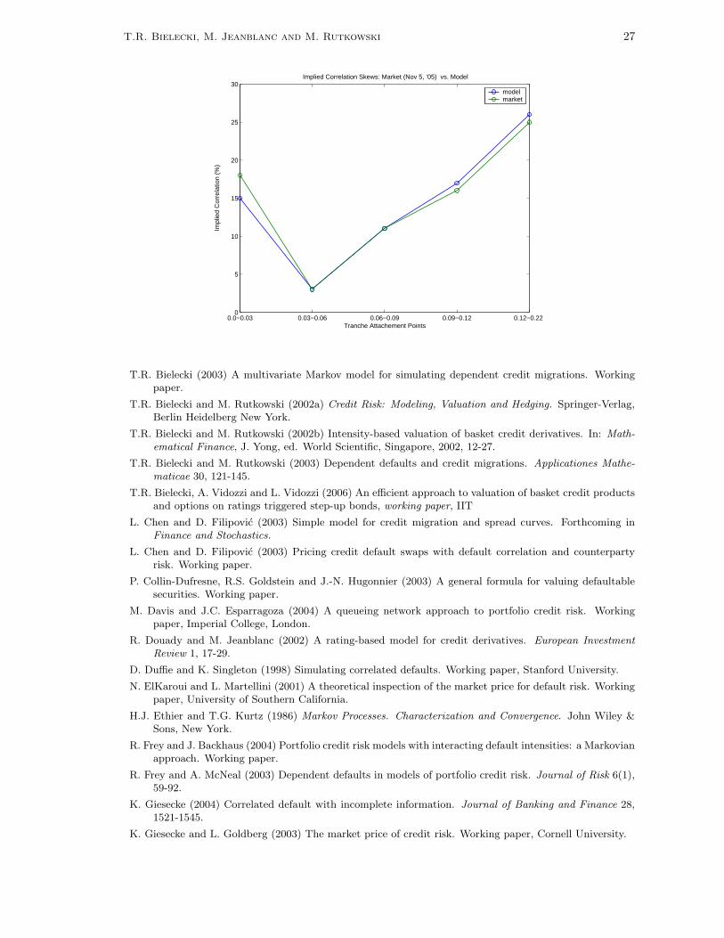
T.R. Bielecki, M. Jeanblanc and M. Rutkowski 27
0.0−0.03 0.03−0.06 0.06−0.09 0.09−0.12 0.12−0.22 0
5
10
15
20
25
30
Tranche Attachement Points
Impl
ied
Cor
rela
tion
(%)
Implied Correlation Skews: Market (Nov 5, ’05) vs. Model
modelmarket
T.R. Bielecki (2003) A multivariate Markov model for simulating dependent credit migrations. Workingpaper.
T.R. Bielecki and M. Rutkowski (2002a) Credit Risk: Modeling, Valuation and Hedging. Springer-Verlag,Berlin Heidelberg New York.
T.R. Bielecki and M. Rutkowski (2002b) Intensity-based valuation of basket credit derivatives. In: Math-
ematical Finance, J. Yong, ed. World Scientific, Singapore, 2002, 12-27.
T.R. Bielecki and M. Rutkowski (2003) Dependent defaults and credit migrations. Applicationes Mathe-
maticae 30, 121-145.
T.R. Bielecki, A. Vidozzi and L. Vidozzi (2006) An efficient approach to valuation of basket credit productsand options on ratings triggered step-up bonds, working paper, IIT
L. Chen and D. Filipovic (2003) Simple model for credit migration and spread curves. Forthcoming inFinance and Stochastics.
L. Chen and D. Filipovic (2003) Pricing credit default swaps with default correlation and counterpartyrisk. Working paper.
P. Collin-Dufresne, R.S. Goldstein and J.-N. Hugonnier (2003) A general formula for valuing defaultablesecurities. Working paper.
M. Davis and J.C. Esparragoza (2004) A queueing network approach to portfolio credit risk. Workingpaper, Imperial College, London.
R. Douady and M. Jeanblanc (2002) A rating-based model for credit derivatives. European Investment
Review 1, 17-29.
D. Duffie and K. Singleton (1998) Simulating correlated defaults. Working paper, Stanford University.
N. ElKaroui and L. Martellini (2001) A theoretical inspection of the market price for default risk. Workingpaper, University of Southern California.
H.J. Ethier and T.G. Kurtz (1986) Markov Processes. Characterization and Convergence. John Wiley &Sons, New York.
R. Frey and J. Backhaus (2004) Portfolio credit risk models with interacting default intensities: a Markovianapproach. Working paper.
R. Frey and A. McNeal (2003) Dependent defaults in models of portfolio credit risk. Journal of Risk 6(1),59-92.
K. Giesecke (2004) Correlated default with incomplete information. Journal of Banking and Finance 28,1521-1545.
K. Giesecke and L. Goldberg (2003) The market price of credit risk. Working paper, Cornell University.

28 Valuation of Basket Credit Derivatives
K. Giesecke and S. Weber (2002) Credit contagion and aggregate losses. Working paper, Humboldt Uni-versity.
J. Gregory and J.-P. Laurent (2004) Analytical approaches to the pricing and risk management of basketcredit derivatives and CDOs. Working paper.
J.C. Hull and A. White (2001) Valuing credit default swaps II. Modeling default correlations. Journal of
Derivatives 8(3), 12-22.
F. Jamshidian (2004) Valuation of credit default swap and swaptions. Finance and Stochastics 8, 343-371.
R.A. Jarrow and F. Yu (2001) Counterparty risk and the pricing of defaultable securities. Journal of
Finance 56, 1765-1799.
M. Kijima (2000) Valuation of a default swap of the basket type. Review of Derivatives Research 4, 81-97.
M. Kijima, K. Komoribayashi and E. Suzuki (2002) A multivariate Markov model for simulating correlateddefaults. Working paper.
M. Kijima and Y. Muromachi (2000) Credit events and the valuation of credit derivatives of basket type.Review of Derivatives Research 4, 55-79.
P.E. Kloeden and E. Platen (1995) Numerical Solution of Stochastic Differential Equations. 2nd ed.Springer, Berlin Heidelberg New York.
H. Kunita and S. Watanabe (1963) Notes on transformations of Markov processes connected with multi-plicative functionals. Memoirs of the Faculty of Science, Kyushu University 17 A, 181-191.
J.-P. Laurent and J. Gregory (2003) Basket default swaps, CDOs and factor copulas. Working paper.
Z. Palmowski and T. Rolski (2002) A technique for exponential change of measure for Markov processes.Bernoulli 8 (6), 767-785
P.J. Schonbucher and D. Schubert (2001) Copula-dependent default risk in intensity models. Workingpaper, University of Bonn.
U. Schmock and D. Seiler (2002) Modeling dependent credit risks with mixture models. Working paper.
F. Yu (2003) Correlated defaults and the valuation of defaultable securities. Working paper.