Valuation of Travel Time

Kenneth A. Small University of California at Irvine

ksmall@uci.edu Sept. 4, 2012

Forthcoming, Economics of Transportation, 1(1), 2012 DOI 10.1016/j.ecotra.2012.09.002

Keywords: value of time; value of reliability; time of day; heterogeneity JEL codes: R41, L91

Abstract

After decades of study, the value of travel time remains incompletely understood and ripe for further theoretical and empirical investigation. Research has revealed many regularities and connections between willingness to pay for time savings and other economic factors including time of day choice, aversion to unreliability, labor supply, taxation, activity scheduling, intra-household time allocation, and out-of-office productivity. Some of these connections have been addressed through sophisticated modeling, revealing a plethora of reasons for heterogeneity in value of time rooted in behavior at a micro scale. This paper reviews what we know and what we need to know. A recurrent theme is that the value of time for a particular travel movement depends strongly on very specific factors, and that understanding how these factors work will provide new insights into travel behavior and into more general economic choices.

Acknowledgement

I am grateful to Mogens Fosgerau, David Hensher, Seiji Steimetz, two referees, and a co-editor of Economics of Transportation for very helpful comments on earlier drafts. Of course, all responsibility remains with the author.

Valuation of Travel Time

Kenneth A. Small

It is difficult to name a concept more widely used in transportation analysis than the

value of travel time. Its theoretical meaning and its empirical measurement are fundamental to

travel demand modeling, social cost analysis, pricing decisions, project evaluation, and the

evaluation of many public policies.

This paper undertakes a selective review of certain aspects, focusing on conceptual issues

and interpretation. Why do we care about the subject, and how does the answer guide our

understanding of it? Despite the importance of value of time in air and freight transportation, I

restrict attention here to surface passenger transportation.

1. Why do we care?

The analysis of value of time is valuable for at least three reasons. First, it is important in

decision making about transportation policy, as just mentioned. Second, it sheds light on broader

questions about human behavior that are of interest throughout economics. Third, it is a crucial

component in travel demand modeling, which is needed for many purposes.

1.1 Investment and policy evaluation

Two of the most prominent goals of transportation investments are time savings and, to a

lesser extent, improvements in the reliability (i.e. predictability) of travel time. Insofar as it is

possible to quantify “typical” costs of travel, travel time and its unreliability tend to dominate.

For example, Small and Verhoef (2007) tally the costs of a typical urban commuting trip in the

United States, finding that travel time and reliability together account for 45% of the average

social variable cost, compared to vehicle capital costs (19%), vehicle operating costs (16%), and

accident costs (16%).

It is not surprising, then, that the majority of investments seek to save travel time by

reducing congestion, raising free-flow travel speed, and/or reducing circuitry of travel. If follows

that the value of those time savings plays a critical role in investment analyses – second only,

1

perhaps, to the assumed discount rate. That value is the sum of the time savings across various

dimensions—trip purposes, user types, times of day, etc.—each multiplied by a “value of time”

(VOT) that captures those particular travelers’ willingness to pay for savings under a particular

circumstance.

As is increasingly recognized, when users face uncertain travel times, they care about the

probability distribution of the travel times they might encounter. Measuring travel-time

reliability amounts to finding a compact way to summarize that distribution, especially its

dispersion. Usually a single summary number is sought, but this is not necessary: travelers could,

for example, care about both the standard deviation and the 90th percentile value, each having a

different implication for the cost of unexpected deviations from a planned travel schedule. Once

we have chosen one or more measures of reliability, we can seek to learn travelers’ willingness

to pay for improvements in those measures – i.e., the value(s) of reliability (VOR).

Investigations into VOT and VOR raise interesting questions. How strongly correlated

are these values with income or wage rate? Is there a stable functional relationship, and if so does

it apply equally across individuals within a country, across time, and across countries? How

much do these values depend on specific situations? For example, do they vary from day to day

even for the same person? Should we expect dramatic changes in VOT resulting from in-vehicle

devices that improve productivity, comfort, or the quality of entertainment en route?

Another question is how one is to understand the relationship between VOT and VOR for

decisions made in the course of a trip, after the uncertainty of travel time is partially resolved.

For example, it is often asserted that a traveler on the way to an airport has a very high VOT.

Presumably this results from a high VOR; but to the traveler who has experienced some delay

and is fearful of more, it may feel like a high VOT. Can this interaction be understood

rigorously? And how does it bear on the value of information that can resolve uncertainty more

quickly?

1.2 Connection to broader behavioral questions

Understanding the value of time can illuminate behavioral puzzles that go well beyond

travel per se. An example is the “harried leisure class,” the revealing title of a small book by

Lindler (1970). As economic development proceeds, one might expect that leisure, a normal

2

good, would be consumed in greater quantities. Yet even as the consumption of leisure goods

from video games to yachts has skyrocketed, people seem more hurried than ever, and in many

countries including the United States they appear to work as hard as ever.1 Consistent with these

observations, measured values of time continue to rise; the theory behind these measurements

helps us understand why leisure might be pursued in a harried manner.

Another puzzle is how people decide on their activity patterns, which in turn would

influence how time-constrained they are in their trips. If most travel is a derived demand, as

usually postulated, then it arises from very complex scheduling decisions in which multiple

activities are sequenced in ways requiring movement among locations. Modeling how people

map out an overlapping set of activity schedules over periods of hours, days, weeks, and even

years, all the time accounting for the ever-changing technologies, costs, and service offerings of

the transportation system, is a daunting challenges to say the least. Nevertheless, many travel

demand researchers believe that only by embedding travel demand into activity choice can trip

scheduling and value of reliability be satisfactory understood.

To complicate the matter further, human genetics appear to have evolved in a context of

constant movement. Thus, it is plausible that people have an inherent desire to be on the move.

How might this show up in values of time for various types of travel? As one example, Ben-

Akiva and Lerman (1985, pp. 174-176) found, using a piecewise linear specification for travel

time, that workers may not care at all about reducing the first 20 minutes of their commute—

perhaps because they like having time between home and office. Mokhtarian and Salomon

(2001) argue, as supported by survey evidence from Ory and Mokhtarian (2005), that a

substantial amount of travel is undertaken for the joy of it rather than as a derived demand.

Yet another puzzle is why students and retirees appear to value their time less than people

in their most economically productive years. One might think a person’s values of time at

different life stages would be equalized via some version of a life-cycle theory of consumption,

despite the fact that time cannot be borrowed like money. This puzzle has potential implications

for how educational services are offered and for the demand for health-care and other services by

older people.

1 More precisely, both paid work and household production work have remained approximately constant over the entire twentieth century in the U.S. These overall statements hide some significant gender-specific changes. See Ramey (2009) and Hammermesh (2012).

3

A warning: some of these questions are not answered or even fully addressed here.

However, one aim of the paper is to show that the theories and empirical techniques used to

address VOT and VOR are capable of being adapted to answer broader questions.

1.3 Travel demand modeling

Even if we cared nothing about VOT or VOR for policy evaluation, we would need to

understand them simply to predict people’s travel decisions. Travel demand models typically

find that travel time is one of the most important explanatory variables in terms of statistical and

economic significance—more consistently so even than cost. Furthermore, the explanatory

power of such models is often improved by judicious interactions of travel time with other

variables such as income, trip distance, and mode. The specification of these interactions

amounts to choosing, explicitly or implicitly, a model of how VOT varies. Thus, it can be guided

by a theory of time allocation aimed at deriving such variations.

A simple example is the early binary probit model of urban commuter mode choice of

Lave (1969). Lave specifies utility to be linear in cost and also linear in travel time multiplied by

the wage rate. The result is that value of time, defined as the tradeoff between time and cost

leaving utility constant, is proportional to the wage rate.2 Train and McFadden (1978) go on to

derive a continuum of specifications leading to the same proportionality, namely that utility is

linear in C⋅w-σ and in T⋅w1-σ, where C and T are cost and travel time, w is the wage rate, and σ is

the elasticity of utility with respect to goods in a simple Cobb-Douglas utility model of choice

between goods and leisure. (Lave’s model is the special case where σ=0.) Thus, one’s beliefs

about an appropriate model of labor-leisure tradeoff can guide the specification of a travel

demand model, with the resulting measurement shedding light on broader questions.3

A recent theme in travel demand modeling is the empirical importance of heterogeneity,

including especially cross-sectional differences in the coefficients that determine VOT and VOR. Some

heterogeneity is “observed,” i.e. explained by measured variables, as in the example just given in which

varying wage rates explain differences in VOT. But empirical models often find that “unobserved”

2 If conditional indirect utility for a mode is V=αC+βTw, where C is cost, T is travel time, and w is wage rate, then VOT is (∂V/∂T)/(∂V/∂C) = (β/α)w. 3 Train and McFadden find their model fits best empirically when 0.7≤σ≤1.0, indicating that a majority of “full income” (unearned income plus potential labor income, less commuting cost) is spent on goods rather than leisure.

4

heterogeneity—that known only through an assumed stochastic distribution of parameters—is much

larger. For example, Small et al. (2005) specify utility linear in cost, travel time, and a measure of

unreliability, with the coefficients on time and unreliability assumed to have normal distributions

(conditional on observed variables such as income or gender); their estimates imply that the resulting

unexplained variance in value of time is several times larger than the variance explained by measured

variables. Of course, this comparison depends on what explanatory variables are included.

This result could mean that significant modeling improvements are possible by finding new

observable explanatory variables. But it may mean that behavior is determined by factors essentially

unknowable to the analyst. If the latter, a further question is: Can we expect the measured properties of

the stochastic distribution describing unobserved heterogeneity to remain stable across time and

locations? The answer—likely to be found in the properties of VOT and VOR—is important to

transferability of travel demand models, which greatly affects the cost of acquiring these very practical

and widely used tools of transportation planning.

2. What do we know?

2.1 Basic results: theory

Most theories of value of time are elaborations of the time allocation framework of Becker

(1965). The basic idea is that people choose how much labor to supply, given a constraint that total time

available is divided among work, leisure, and travel. At its bare bones, this model implies that travel time

is valued at the after-tax wage rate. This is because the Becker model assumes that time can be transferred

freely between work and leisure, so any marginal savings in travel time can be used to increase labor

income. If the individual is optimizing, it is sufficient to know its value in that activity to determine the

marginal tradeoff between travel time and money.

This model has been elaborated in many directions. A common starting point is DeSerpa (1971).4

Utility U is affected by goods consumption G, by times Tk. spent in each of K other activities (which can

include both travel and leisure pursuits), and by time Tw spent at work (which may increase or decrease

utility). Each activity has a minimum time requirement, kT (hence constraint kk TT ≥ ), plus there is

4 Here I follow the exposition of Small and Verhoef (2007, sect. 2.6.1). For reviews of additional theoretical developments, see González (1997), Jara-Díaz (2000, 2007), and Hensher (2011).

5

also an overall time constraint, TTTk

kw ≤+∑ . The budget constraint is , where Y

is unearned income and the price of goods consumption is normalized at one.

wwTYG +≤

This problem can be solved by formulating a Lagrangian function, in which each

constraint is associated with a Lagrange multiplier indicating how tight it is (i.e., the rate at

which utility could be increased by relaxing it a little). Let λ, μ, and φk be the Lagrangian

multipliers for the budget constraint, the overall time constraint, and the activity-specific time

constraints, respectively. We define the value of travel time as the marginal tradeoff between

travel time and unearned income that would leave the traveler indifferent:

λφKK

VK

KT YV

TVTd

dYv =∂∂∂∂

−=⎟⎟⎠

⎞⎜⎜⎝

⎛≡

//

(1)

where V is the indirect utility function (the utility achieved in the solution to the problem), and K is the

label for the activity consisting of traveling.5 The last equality follows from the properties of Lagrangian

multipliers. The solution to the optimization problem yields:

λ

UUw

λU

λμ

v TKTwTKKT

−+=−= (2)

where UTK and UTw are marginal direct utilities of time spent in travel and at work, respectively.

Equation (2) has a natural interpretation which aids thinking about empirical

specifications for value of time. The first equality in (2) tells us that the value of travel time is

determined by the relative tightness of time and budget constraints (indicated by μ/λ), modified

by any enjoyment or dislike of the travel itself (UTK). We can think of μ/λ as a pure time value,

sometimes called the “value of time as a resource,” since it indicates the monetary value of

increasing the total time available.6 The second equality in (2) tells us further that the value of

travel time is greater or less than the wage rate depending on whether work is liked or disliked

relative to travel, i.e. on the sign of UTw-UTK. An empirical finding that VOT is less than the

5 The value of λ can be estimated using Roy’s identity provided the model includes a variable measuring the monetary cost of travel (Small and Verhoef, 2007, equation 2.24). Even if income appears in the travel choice model, its coefficient would not measure ∂V/∂Y because other portions of the indirect utility function, namely all those unaffected by the choice being analyzed, contribute to ∂V/∂Y but are necessarily omitted from the travel choice model.

6 That is, YVTV

λμ

∂∂∂∂

=// .

6

wage rate can then be taken as evidence that people dislike work more than traveling.7 Jara-Díaz

et al. (2008) provide more direct evidence for this interpretation, as they develop a method to

separately estimate the value of travel time and the value of leisure μ/λ. Doing so for samples

from three different nations, they achieve insights about possible cross-country differences in the

disutility of time at work.

KTv

Can workers freely alter their work hours, as posited above? Evidence shows that they

often must change jobs to accomplish this, so that limitations on job mobility constrain work

hours to some extent (Altonji and Paxson, 1992). One way to address this is to assume that wage

w depends on time worked Tw, in which case an added term Tw⋅(dw/dTw) appears on the right of

(2).8 Or one could assume a rigid work-hours constraint, ww TT = , with associated Lagrangian

multiplier φw. This modification adds a term φw/λ to the value of time as given by (2), thus

raising VOT if people are forced to work more than they want and lowering it if they work less

than they want. These results are intuitive: if people are either enticed or required to work more

than they want to given the prevailing wage rate, they perceive their time as more scarce and

hence more highly valued.

This theory can be elaborated to deal with many possible variations of VOT with trip

purpose, income, gender, family status, and other factors. For example, for a person with large

exogenous time commitments, the overall time constraint will bind more tightly, all else equal,

so that μ/λ in (2) is larger; this may be one reason why longer trips seem empirically to have

higher VOT (Daly and Carrasco, 2009). Another reason could be that trips become more

tiresome the longer they are, so that increasing marginal disutility (-UTK/λ) sets in, thereby

raising VOT according to (2). As another example, Johnson (1966) posits that people with higher

wages also tend to have more enjoyable jobs, perhaps causing the value of time to vary more

than proportionally with the wage rate since the effect of UTw/λ in (2) will then rise with the

wage rate. Yet another example is when travel time is decomposed into various components such

as in-vehicle, walking, and waiting for a transit trip, or such as congested and uncongested time

7 This effect could be strong enough to drive VOT to zero, as posited by Mokhtarian and Salomon (2001). In that case, the constraint KK TT ≥ is not binding and travel would be what DeSerpa calls a pure leisure good.

8 This can be seen as replacing the average compensation w by the marginal compensation [w+Tw⋅(dw/dTw)] as the measure of the economic cost of lost time.

7

for an automobile trip. It is typically postulated that walking, waiting, and congested time are

onerous compared to their in-vehicle or uncongested counterparts, in which case a simple

generalization of (2) shows that these components of travel will exhibit higher values of time.

Other hypotheses, described later, require greater generalizations of the model.

For business travel, it is natural to turn instead to production theory.9 Formulating how a

firm’s profits are affected by employees’ time spent in business travel, Hensher (1977) derives

an intuitive equation for value of time savings consisting basically of four additive components.

First is marginal product of the time savings to the employer if that time were spent instead at the

office, but modified by subtracting the portion of travel time that is spent working (perhaps at

reduced productivity). Second is the utility of time if it were spent at work, UTw. Third is the

value to the traveler of the portion of travel time perceived as leisure (this portion is also

subtracted from travel time when computing components one and two). Fourth is a quantity

reflecting reduced productivity at work due to fatigue from traveling. The second and third

components are further corrected to account for personal income taxation. In practice, the use of

this formula is hampered by lack of data on some items, so certain parts are typically omitted,

namely personal income taxation, productive time while traveling, and the effects of fatigue.

This brief sketch of the production approach to business travel reveals a conclusion that

applies to other forms of travel as well. The value of time that affects travel decisions can depend

strongly on factors that analysts normally do not observe: individual tax rates, ability to use

travel time productively, fatigue from travel, enjoyment of work, tightness of work-hours

constraints, and many others. It is no surprise, then, that studies often reveal wide variations in

measured value of time, depending on the particular way the studies are formulated.

2.2 Basic results: empirical

The empirical literature is vast; here I extract a few points from the many reviews

available such as Small and Verhoef (2007, ch. 2) and Hensher (2011), as well as from the meta-

analyses by Shires and de Jong (2009) and Abrantes and Wardman (2011).

9 Here I follow the concise presentation of Hensher (2011, pp. 139-141).

8

First, the value of time for commute trips seems typically to average around one-half the

gross wage rate—amazingly close to the early results of Lave (1969). Values also vary widely by

trip purpose, typically being highest for business travel and lowest for discretionary leisure

travel.

Second, values rise with income or wage rate, but less than proportionally—in contrast to

the theory by Johnson (1966) just noted. This variation is well documented in cross-sections

(especially across nations) and over time, although not necessarily with identical elasticities. For

example, the meta-analysis of Abrantes and Wardman (2011) measures the income elasticity of

VOT to be 0.9, based on variations over time within the UK; but studies with mainly cross-

sectional variation typically yield elasticities on the order of 0.5.10 Gunn (2001) finds some

evidence that VOT has undergone a secular downtrend independent of income—perhaps due to

improved in-vehicle amenities—which could cause some studies to underestimate the income

elasticity by confounding income with this secular trend. Another wrinkle is that the relationship

of VOT to income at any point in time may not be one of constant elasticity: Börjesson et al.

(2012), using repeated cross-sections, find that the income elasticity is close to zero at low

incomes and considerably greater than one for higher incomes. If confirmed in other data sets,

such a dramatically non-constant income elasticity of VOT would have important implications

for the distribution of costs and benefits from various policies.

Third, there are some well-established differences among values of time spent under

various circumstances. Automobile drivers value time more highly under congested conditions

than under free-flow conditions, by perhaps 25% to 55%.11 (As discussed later, one explanation

for this is the additional effort required by drivers to avoid accidents in congested conditions.)

The value of walking or waiting time on transit trips is considerably larger than that of in-vehicle

time—by multiples of two to three by most assessments, although the multiple is only 1.7 in

Abrantes and Wardman (2011, Table 13). Abrantes and Wardman also find an elasticity of VOT

with respect to distance of 0.16 (p. 10).

10 For example, Wardman (2004). See Hensher (2011, pp. 143-146) and Shires and de Jong (2009) for thorough reviews. Shires and de Jong (2009) measure elasticities with respect to gross domestic product per capita, which they believe are driven mainly by cross-sectional variations, of roughly 0.7 for commuting and 0.5 for business and leisure travel. Gunn (2000, p. 444) concludes that the evidence supports a cross-sectional elasticity of 0.5.

11 Based on results reported by Abrantes and Wardman (2011, p. 7) Hensher (2011, Table 7.1), and Rizzi et al. (2012). Interestingly, Rizzi et al. find that the congestion premium appears in their stated preference data only when pictures of congestion are included in the questions posed to survey respondents.

9

Since VOT is typically measured as a ratio of coefficients, its standard error requires an

additional calculation. The simplest method, known as the Delta method, applies a first-order

Taylor series approximation to deviations around the point estimate, which is the ratio βt/βc of

point estimates of coefficients:

( )( )

( )( )

( )( )

( )ct

ct

c

c

t

t

ct

ct CovVarVarVarββββ

ββ

ββ

ββββ ,

2/

/222 −+≅ .

Daly et al. (2012) show that if βt and βc are maximum likelihood estimators of the coefficients,

then this approximation is the maximum likelihood estimator for their ratio, so that it is

asymptotically consistent just as are the standard estimates of the variances and the covariance of

the individual coefficients. Thus there is often no need to apply more complex methods, such as

Monte Carlo simulation, which are analyzed by Armstrong et al. (2001).12 However, simulation

may be necessary in more complex models that include error components or in which the value

of time is a more complex function of coefficients.

2.3 Heterogeneity and mixture models

In addition to the observed heterogeneity just documented, newer econometric techniques

have permitted researchers to measure the remaining unexplained variation, known as

“unobserved heterogeneity.” The primary technique is the mixed discrete choice model, in which

utility has an error term with two components: the usual one whose distribution defines a

particular class of discrete-choice models (such as probit, logit, or generalized extreme value),

plus a second component that depends on the data and can have a very general distribution.13

For example, a mixed logit model begins with a conditional indirect utility function

depicting the value to consumer i of choosing an alternative j having observable characteristics

represented by vector zj:

12 The Delta method applies also to a much more general class of functions of coefficient estimates, as explained by Daly et al. (2012) with many examples calculated in their Table 1.

13 Walker and Ben-Akiva (2011) provide a compact review. Train (2009) provides detailed information about estimation methods, including reasons to prefer using non-random draws (such as from a Halton sequence) for the simulations.

10

ijijijijjij zzV ενβα ++′+= )(0 (3)

where εij is a pure random term with an extreme value distribution (hence “logit” in the model’s

name) and νij is another random variable with some “mixing distribution,” so called because the

resulting choice probabilities are integrals involving a mixture of the two distributions. Common

distributions assumed for νij include normal, half-normal, log-normal, and triangular—the latter

three often chosen in order to restrict coefficients to have the theoretical expected signs.

Estimation involves Monte Carlo simulation to approximate the expected choice probabilities

derived from (3), taking advantage of the simplicity of the logit formula for the choice

probability conditional on a random draw from the mixing distribution. Compiling results for

many random draws provides simulated probabilities for choices, which are approximations to

probabilities computed by integration over the two random distributions. From the simulated

probabilities, one forms the simulated log-likelihood function, maximization of which provides

estimates of the parameters β0 and the “hyperparameters” σ of the mixing distribution.

McFadden and Train (2000) derive some general properties of this model.

The most commonly assumed functional form for νij(⋅) depicts pure randomness in the

coefficients βk of particular variables, zk, in (3):

∑=k

kijkkij zφσν

where φk is a standardized random variable with the postulated mixing distribution,14 σk is the

standard deviation of that distribution, and is the value taken by the k-th variable in data

vector z. Equivalently, the coefficient vector β is now viewed as random, with k-th component

+σ

kijz

k0β kφk. Thus σk can be considered a measure of dispersion in the k-th coefficient as it varies in

an unobservable fashion across the population.15 Allowing in addition for correlations among the

random components, the model can be written:

ijijjij zV εβα +′+=

14 That is, φk is the postulated random variable after subtracting its mean and dividing by its standard deviation.

15 In general these random components can be correlated, with their variance-covariance matrix parameterized by a vector σ. A special case of (3) involves variables dk that are just combinations of alternative-specific constants, defined as one if j is included in a particular combination indexed by k, and zero otherwise. Brownstone and Train (1999) show how this formulation can capture correlations among alternatives similar to those assumed in a nested logit model.

11

where β is random with mean β0 and variance-covariance matrix parameterized by some vector

σ.

In the context of VOT, one typically specifies travel time, reliability, and/or cost to be

variables with random coefficients. Estimating parameters β0 and σ then permits calculation of

all the properties of the distribution of VOT. This calculation can be combined with observed

heterogeneity, which arises from interacting time, reliability, and/or cost with other observed

variables (like income or trip distance). It can also be combined with the sampling error,

summarized in the standard errors of estimated parameters, to obtain the overall uncertainty in

VOT or in value of reliability; Small et al. (2005) do this in order to compute percentiles of the

distribution of VOT. They find that the greatest source of variation is unobserved heterogeneity,

i.e. variation due to the random variables φk.

However, there are at least two significant barriers to successful use of mixed discrete

choice models for measuring values of time. Both are amenable to amelioration, but at some

cost.

Choice of distribution function. The first barrier is the fact that the assumed distribution

function for the random coefficients can strongly influence the resulting coefficient estimates,

and in particular such ratios as VOT.16 The main reason is that commonly used tractable

distribution functions vary greatly from one another in the size of their tails, i.e. in the

probabilities of large deviations from central values. Data are usually sparse or entirely absent in

that region, making it difficult or impossible to determine what distribution best represents the

data there. 17

One way to avoid assuming an inappropriate mixing distribution is to estimate part of it

nonparametrically. Fosgerau (2006) obtains promising results this way, demonstrating along the

way that the distribution’s tails are not necessarily identified in a given data set. A possibly more

parsimonious approach is the latent class model: assume that the mixing distribution involves

16 Hess et al. (2005), Fosgerau (2006), and Fosgerau and Bierlaire (2007) provide comparisons among results for various parametric, semiparametric, and seminonparametric distributions using both actual and artificially generated data.

17 Several of these distributions are censored so to require VOT≥0, with a probability mass at VOT=0 representing people who don’t care about travel time. Axhausen and Cirillo (2006) fit several models showing a positive fraction of travelers having zero or even negative values of time, and argue that this is theoretically plausible.

12

just a few possible values of the parameter vector, each characterizing a latent (i.e. unobservable)

class of travelers into which survey respondents are assigned probabilistically depending on their

characteristics (Greene and Hensher, 2003).

Implausible distributions of ratios. Another difficulty with mixed models is their

tendency to produce implausibly dispersed distributions for ratios of coefficients, which often

represent the willingness to pay (WTP) for a characteristic such as travel time. The problem is

especially acute if the denominator of the ratio—typically the coefficient of a price variable—is

allowed to be random with a distribution whose support includes very small values (for example,

a log-normal distribution). For this reason, the cost coefficient is often specified as non-random

even if this assumption is contradicted by a statistical test.

An alternative specification reparameterizes utility in “WTP space” so that the assumed

randomness occurs in the ratios themselves. For example, we could rewrite (3) as:

ijijijjij zpV εγλλα +′++= − (4)

where p denotes price and z- denotes the vector of all other variables. The model is now

nonlinear in parameter λ and parameter vector γ, the latter consisting of direct estimates of WTP.

This does not diminish the model’s computational tractability because probabilities conditional

on random parameters still have the usual formulas (e.g. logit if ε has the double-exponential

distribution), and the joint distribution of the random parameters themselves is estimated using

Monte Carol simulation. Train and Weeks (2005) and Hensher and Greene (2011) report that

such models produce much smaller dispersion in WTP measures such as VOT. However, they

also report that the model in WTP space does not fit the data as well as the model as more

usually formulated (i.e. in “coefficient space”). The particular models studied by these authors

have complexities that make it difficult to draw a firm conclusion about the significance of this

last finding.18

18 Train and Weeks estimate some coefficients using a log-normal distribution, with apparently good results in terms of conventional statistical significance (i.e., high t-ratios). However, when they calculate the implied estimated values of the direct “coefficient” of the variable of interest, e.g. ∂V/∂p, none of the resulting values are statistically significant for either the model in preference space or that in WTP space. Hensher and Greene’s WTP-space model has four fewer parameters than their preference-space model, due to restricting the random parameter related to the price coefficient to be uncorrelated with other random parameters— probably a useful restriction from the point of view of statistical power. This restriction may explain why their model in WTP space fits the data less well.

13

Conclusion on Mixed Discrete Choice Models. It seems clear that heterogeneity in values

of time exists, and that an important part of it will always be beyond our ability to explain using

observable data. Mixture models provide information on this heterogeneity and so seem certain

to continue as a necessary tool. The problem is that the new information needed must describe

joint distributions of an unknown form, a task beyond many data sets. To put it more formally,

new information can be obtained from a statistical model only at a cost in terms of statistical

power, i.e., the ability of a given data set to precisely estimate parameters of interest. While it

may be tempting to estimate a very general model, based on the ability to reject simpler ones,

this also produces the danger of overfitting. In practice, one must always keep an eye out for

signs that desired parameters are simply not well identified in a given data set, in which case

some theoretically based restriction may be called for.

2.4 Time of day variation, scheduling choice, and reliability

One source of heterogeneity in value of time is the time of day of travel. Generally, VOT

is found to be higher in peak hours than off-peak, although this may reflect unmeasured

differences in trip purposes. But what about the effects on VOT of small differences in departure

or arrival times?

2.4.1 Scheduling choice and the value of time

Even defining VOT is ambiguous if congestion is changing rapidly at the times during

which a trip takes place. This is because travelers may adjust their departure times to meet

scheduling goals, thereby making the travel time endogenous. For example, suppose the trip

takes place during the rising part of the rush hour, and an improvement to the last link used

lowers its (exogenous) travel time by one minute. Suppose also the traveler has been optimizing

her departure time in a continuous fashion to meet certain scheduling preferences. Then in

response to the improvement, she may further adjust the departure time; this will cause only a

second-order utility change (due to the envelope theorem), so it is appropriate to apply the usual

VOT analysis to the one-minute time saving. But if the traveler is at a corner solution, such as

14

needing to maintain a fixed arrival time, the departure-time adjustment will result in

encountering more congestion and thus utility will rise by less than the standard calculation.

We can better understand the connection between scheduling and VOT by considering

travelers’ preferences concerning scheduling. Vickrey (1969) postulates “alpha-beta-gamma”

preferences, in which a commuter wishes to arrive exactly at t*, suffering a scheduling cost at

rate β per minute for early arrival or γ per minute for late arrival. Travel time is valued at α. If

congestion is changing rapidly, it becomes optimal for some travelers to suffer scheduling cost in

order to reduce their travel-time cost. This balance changes if an exogenous transportation

improvement reduces travel time at any given time of day. Furthermore, congestion occurs as a

result of these scheduling decisions, in a pattern that will itself shift due to the exogenous change

in conditions. Thus, to fully analyze the outcome as well as the benefits in a situation of rapidly

changing congestion, a model of scheduling decisions and resulting equilibria is needed. Newell

(1987) provides a rather general such model; a special case is the “bottleneck model,” which

postulates identical travelers with alpha-beta-gamma preferences, and congestion determined by

a deterministic queue behind a fixed-capacity bottleneck.19

Where might alpha-beta-gamma preferences come from? And might they vary by time of

day as well? Vickrey (1973) provides a key theoretical insight, elaborated by Tseng and Verhoef

(2008) and de Palma and Fosgerau (2011). Suppose, for concreteness, a commuter has time-

varying preferences for when he conducts activities at home and at work. Perhaps he wants to

sleep while it is dark, to interact with children at breakfast, and to be at work when the presence

of others makes it the most productive to do so.20 From the traveler’s individual point of view,

this situation can be described by a time varying rate of utility spent at each location. Following

Tseng and Verhoef, let H(t) and W(t) represent the value of a unit of time spent at home or work,

respectively, at time t (relative to spending that time traveling); and let T be the travel time

between home and work. If H′(t)<W′(t+T) within a relevant solution region, the worker’s choice

will be to choose a departure time td for which H(td)=W(td+T)≡H* because this equalizes the

19 The bottleneck model was first described by Vickrey (1969), and further developed by several authors, especially Fargier (1983), Arnott et al. (1990, 1993, 1998). Alpha-beta-gamma preferences were measured empirically for a sample of commuters by Small (1982).

20 Henderson (1981) and Fosgerau and Small (2012) provide formal equilibrium models of agglomeration in the home and/or workplace that could lead to such apparent preference. Wilson (1988) provides empirical evidence for the productivity benefit of working simultaneously with others.

15

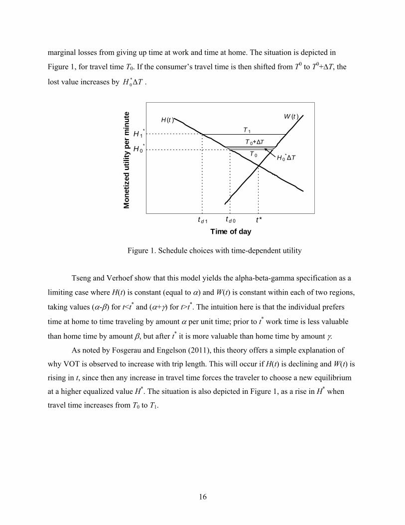
marginal losses from giving up time at work and time at home. The situation is depicted in

Figure 1, for travel time T0. If the consumer’s travel time is then shifted from T0 to T0+ΔT, the

lost value increases by . TH Δ*0

Time of day

Mon

etiz

ed u

tility

per

min

ute

T 0

T 0+ΔT

T 1

H (t ) W (t )

H 0*

H 1*

t d 1 t d 0 t *

H 0*ΔT

Figure 1. Schedule choices with time-dependent utility

Tseng and Verhoef show that this model yields the alpha-beta-gamma specification as a

limiting case where H(t) is constant (equal to α) and W(t) is constant within each of two regions,

taking values (α-β) for t<t* and (α+γ) for t>t*. The intuition here is that the individual prefers

time at home to time traveling by amount α per unit time; prior to t* work time is less valuable

than home time by amount β, but after t* it is more valuable than home time by amount γ.

As noted by Fosgerau and Engelson (2011), this theory offers a simple explanation of

why VOT is observed to increase with trip length. This will occur if H(t) is declining and W(t) is

rising in t, since then any increase in travel time forces the traveler to choose a new equilibrium

at a higher equalized value H*. The situation is also depicted in Figure 1, as a rise in H* when

travel time increases from T0 to T1.

16

2.4.2 Scheduling costs and the value of reliability

How does a traveler come to value reliability? Earlier papers have identified scheduling

preferences as the main reason people want predictable travel times.21 The traveler suffers not

only the occasional costs of unexpected delays, but also suffers some routine costs of choosing

an earlier schedule in order to allow a safety margin. Since the precise costs are not known in

advance, the travelers is usually assumed to chose a departure time that minimizes the expected

value of the sum of these costs, taking into account whatever is known about the distribution of

travel times.

Fosgerau and Karlström (2010) provide explicit expressions for the resulting costs, using

alpha-beta-gamma preferences, in the case where congestion is not changing over time. It’s

worth going through the mathematics for the insights we get concerning appropriate measures of

reliability.

We wish to find the traveler’s cost as a result of changes in the mean travel time or in

measures of the dispersion of its distribution. To do so, first consider the traveler’s optimization

problem. Let F(T) be the cumulative distribution function of random travel times T, with mean μ

and standard deviation σ. Normalizing the time axis so that t*=0, it is convenient to define

departure by the lead time D=-td, so that arrival time is T-D and early arrival (arriving before t*)

occurs if T-D<0. Then scheduling costs are -β⋅(T-D) for early arrival and γ⋅(T-D) for late arrival.

Travel time cost is αT. Taking expectations, the consumer’s decision problem is therefore:

( ) ( )

( ) ( ) ( ) dTTFDTD

dTTFDTdTTFDTECMin

D

D

DD

)('

)(')('

∫∫ ∫

∞

∞−

∞

−++−+=

−+−−=

γβμβαμ

γβαμ

where μ is the mean travel time. The solution turns out to be surprisingly simple and

enlightening. The first-order condition for minimizing expected cost is:

21 For summaries, see Bates et al. (2001) and Li et al. (2010). Most empirical attempts to measure a “planning cost” as an additional cost to unpredictability, once scheduling costs are accounted for, have obtained small and statistically insignificant results (Noland et al., 1998). However a meta-analysis by Tseng (2008) finds some evidence for such planning costs: when scheduling costs are included separately the reliability coefficient is reduced by about 80 percent, but not by 100 percent, compared to when a single reliability variable is included without scheduling cost.

17

** )(1 LPDFγβ

β≡−=

+

where D* is optimal lead time (time allowed between departure and preferred arrival) and is

the probability of arriving late. This result shows that, remarkably, the optimizing traveler sets

to a value that is entirely independent of the travel-time distribution.

*LP

*LP

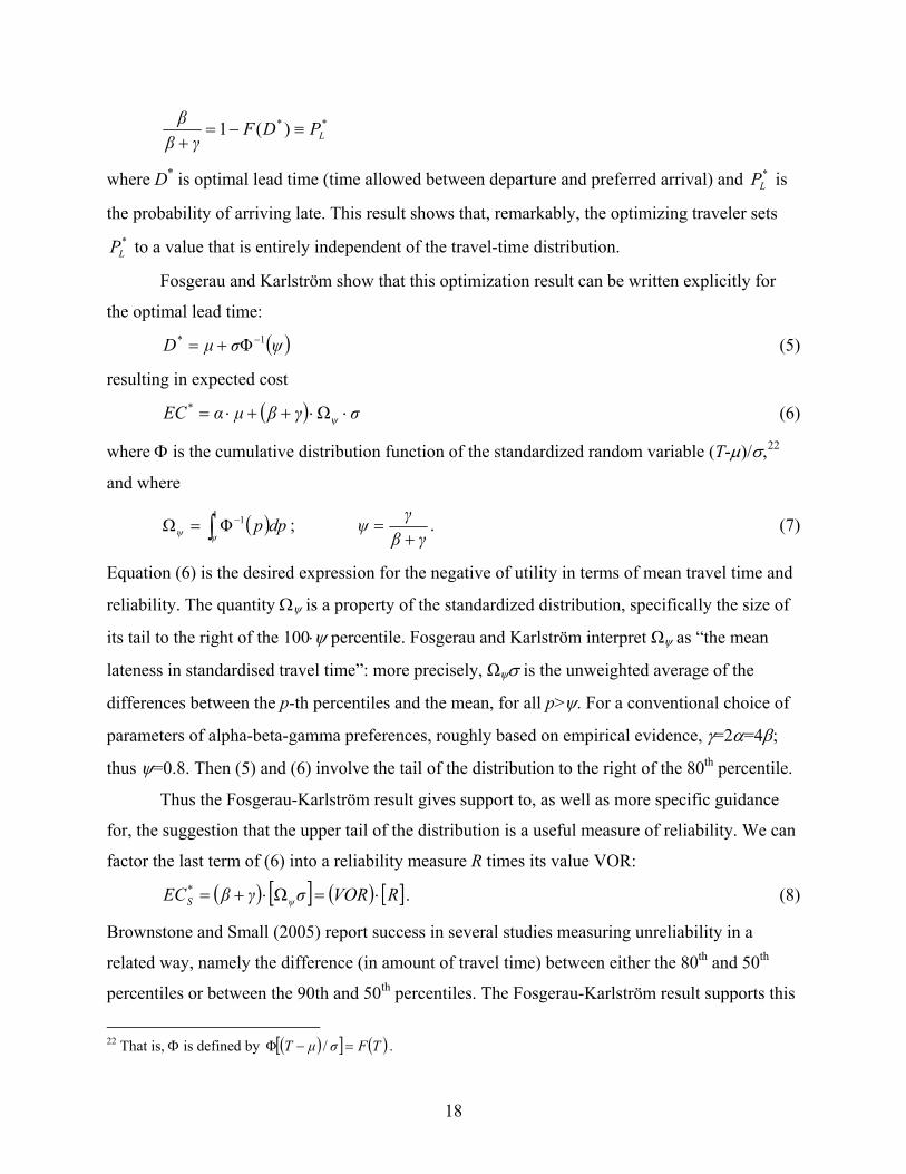
Fosgerau and Karlström show that this optimization result can be written explicitly for

the optimal lead time:

(5) ( )ψσμD 1* Φ−+=

resulting in expected cost

(6) ( ) σγβμαEC ψ ⋅⋅++⋅= Ω*

where Φ is the cumulative distribution function of the standardized random variable (T-μ)/σ,22

and where

; ( )∫ −=1 1ΦΩψψ dpp

γβγψ+

= . (7)

Equation (6) is the desired expression for the negative of utility in terms of mean travel time and

reliability. The quantity Ωψ is a property of the standardized distribution, specifically the size of

its tail to the right of the 100⋅ψ percentile. Fosgerau and Karlström interpret Ωψ as “the mean

lateness in standardised travel time”: more precisely, Ωψσ is the unweighted average of the

differences between the p-th percentiles and the mean, for all p>ψ. For a conventional choice of

parameters of alpha-beta-gamma preferences, roughly based on empirical evidence, γ=2α=4β;

thus ψ=0.8. Then (5) and (6) involve the tail of the distribution to the right of the 80th percentile.

Thus the Fosgerau-Karlström result gives support to, as well as more specific guidance

for, the suggestion that the upper tail of the distribution is a useful measure of reliability. We can

factor the last term of (6) into a reliability measure R times its value VOR:

( ) [ ] ( ) [ ]RVORσγβEC ψS ⋅=⋅+= Ω* . (8)

Brownstone and Small (2005) report success in several studies measuring unreliability in a

related way, namely the difference (in amount of travel time) between either the 80th and 50th

percentiles or between the 90th and 50th percentiles. The Fosgerau-Karlström result supports this

22 That is, Φ is defined by ( )[ ] ( )TFσμT =− /Φ .

18

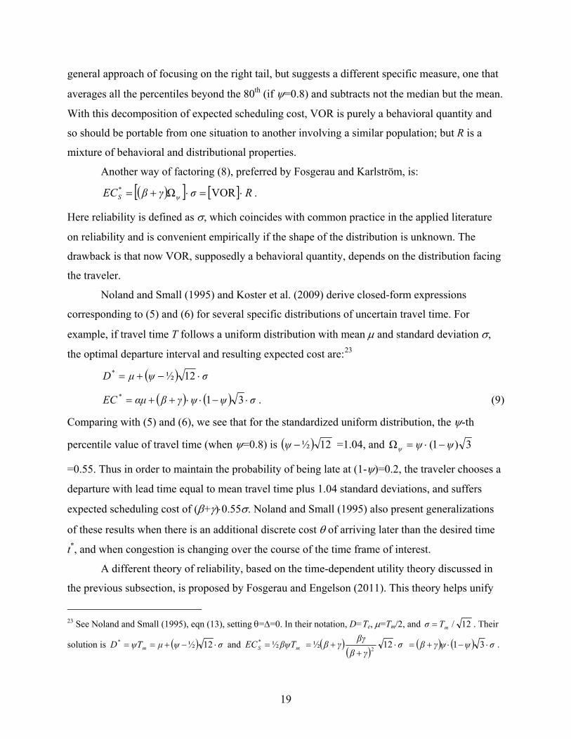
general approach of focusing on the right tail, but suggests a different specific measure, one that

averages all the percentiles beyond the 80th (if ψ=0.8) and subtracts not the median but the mean.

With this decomposition of expected scheduling cost, VOR is purely a behavioral quantity and

so should be portable from one situation to another involving a similar population; but R is a

mixture of behavioral and distributional properties.

Another way of factoring (8), preferred by Fosgerau and Karlström, is:

( )[ ] [ ] RσγβEC ψS ⋅=⋅+= VORΩ* .

Here reliability is defined as σ, which coincides with common practice in the applied literature

on reliability and is convenient empirically if the shape of the distribution is unknown. The

drawback is that now VOR, supposedly a behavioral quantity, depends on the distribution facing

the traveler.

Noland and Small (1995) and Koster et al. (2009) derive closed-form expressions

corresponding to (5) and (6) for several specific distributions of uncertain travel time. For

example, if travel time T follows a uniform distribution with mean μ and standard deviation σ,

the optimal departure interval and resulting expected cost are:23

( ) σψμD ⋅−+= 12½*

( ) ( ) σψψγβαμEC ⋅−⋅⋅++= 31* . (9)

Comparing with (5) and (6), we see that for the standardized uniform distribution, the ψ-th

percentile value of travel time (when ψ=0.8) is ( ) 12½−ψ =1.04, and 3)1(Ω ψψψ −⋅=

=0.55. Thus in order to maintain the probability of being late at (1-ψ)=0.2, the traveler chooses a

departure with lead time equal to mean travel time plus 1.04 standard deviations, and suffers

expected scheduling cost of (β+γ)⋅0.55σ. Noland and Small (1995) also present generalizations

of these results when there is an additional discrete cost θ of arriving later than the desired time

t*, and when congestion is changing over the course of the time frame of interest.

A different theory of reliability, based on the time-dependent utility theory discussed in

the previous subsection, is proposed by Fosgerau and Engelson (2011). This theory helps unify

23 See Noland and Small (1995), eqn (13), setting θ=Δ=0. In their notation, D=Te, μ=Tm/2, and 12/mTσ = . Their

solution is ( ) σψμTψD m ⋅−+== 12½* and mS TβψEC ½* = ( )( )

σγβ

βγγβ ⋅

++= 12½

2 ( ) ( ) σψψγβ ⋅−⋅+= 31 .

19

the understanding of time-varying VOT, scheduling choice, and value of reliability. They assume

that the value functions H(t) and W(t) are linear in t (as shown in Figure 1). This leads to two

striking results, both of practical interest. First, VOT varies with trip length in a simple way: it is

a linear function of travel time T, increasing or decreasing in T depending on whether the slopes

of H and W are of opposite or the same signs. Second, if reliability is measured as σ, VOR is a

constant, equal to the slope W′, which may be interpreted as the incremental cost of losing time

at the destination. An empirical study by Tseng and Verhoef (2008, Fig. 3), using responses by

Dutch commuters to hypothetical scenarios, suggests that the assumption of linear H and W is a

reasonable approximation.

How big is VOR? Li et al. (2010) review both theoretical and empirical aspects of value

of reliability.24 Among other things, they report on measurements of the reliability ratio, defined

as the ratio of VOR to VOT when reliability is measured as σ. For the uniform distribution,

equation (9) shows that the reliability ratio is ( ) ( ) αψψγβ /13 −⋅+⋅ , or 0.69 with conventional

parameter values mentioned earlier. According to Li et al., this ratio is most often found

empirically to be between 0.8 and 1.3 for car travel, with somewhat higher values for travel by

public transportation. Tseng (2008) obtains a higher value, namely 1.71, from a meta-analysis of

VOR studies, when both scheduling and planning motivations are lumped together in a single

value. Li et al. suggest that the measured reliability ratio is sensitive to the different ways

researchers have used to describe hypothetical distributions of uncertain travel times to survey

respondents.

2.4.3 Decisions en route and the value of information

From the theories just presented, we see that anything that reduces the dispersion in the

distribution of random travel times reduces scheduling cost. Making traffic information available

before the scheduling decision is made is one such measure to reduce dispersion. But what about

information provided en route, including information inherent in the travel time actually

experienced on portions of the trip already taken?

24 Other reviews include Bates et al. (2001), Noland and Polak (2002) and Batley et al. (2008), the latter being especially comprehensive.

20

Usually it is too late to alter the scheduling of the trip once it has begun, unless the

traveler should decide to make a stop along the way. But it may not be too late to influence some

route or mode decisions. For example, one could decide to substitute transit for the last portion of

a car trip, or taxi for the last leg of a transit trip. Given the heavy investment cost of information

systems, it could well be worthwhile to build such an explicit model of such a process, despite its

complexity and the need for fine-grained information.

At any point in the trip, such subsequent decisions may involve tradeoffs among expected

travel time savings, their dispersion, and cost. Thus, one could consider the revealed preferences

as exhibiting real-time variations in VOT and VOR, depending strongly on scheduling goals.

This is the germ of truth in claims like “the value of time is very high when going to the airport.”

But is it useful to look at the problem this way? Transportation investments cannot be made in

real time, so knowing about such variations is of little help for planning. In principle it could

influence real-time decisions in traffic control centers, but it would be impossible to know the

specific scheduling constraints facing the thousands of travelers affected. Thus, it’s probably best

to recognize that the high values of time that people may feel introspectively as they travel are

really reflections of value of reliability.

Information provision has the potential not only to reduce travel-time dispersion for

individuals, but to change the pattern of congestion itself. This is because if large numbers of

travelers are induced by real-time information to change their decisions, this will change where

and when congestion occurs. A number of models suggest that it is helpful, from a network point

of view, to have some fraction of travelers informed about where congestion is severe, but also

that if market penetration of such a system exceeds some threshold, everyone may be made

worse off. The reason is mainly overreaction: unless the information is extremely accurate,

traffic tends to move to a few alternative routes which then become too congested.25 Basically

this is a market failure due to herd effects; it tends to be quite specific to the situation modeled

and assumptions made. The failure is less likely if there are alternate sources of information

available, if different travelers react differently to their information, and if the information is

presented in such a way as to encourage some randomness in response—rather like mixed

strategies in game theory.

25 For examples, see Arnott et al. (1991), Ben-Akiva et al. (1991), and Emmerink et al. (1994, 1998).

21

Making the information accurate is extremely challenging, because it requires predicting

congestion for the duration of a traveler’s trip. This in turn requires correctly modeling the

behavior of travelers in response to unanticipated congestion and to the information itself. Yang

(1998) and Paz and Peeta (2009) develop formal models of such a system.

2.5 Stated preference data

As theory and practice have moved to more fine-grained analyses of preferences, it has

become increasingly difficult to measure the needed parameters using data on actual choices

made by travelers. These data, known as “revealed preference” (RP), are often considered

inherently superior to other sources because they depict choices made in real-world situations

where unknowable factors influence decision makers, where good decision making is motivated

by actual gains and losses, and where repeated choices provide more opportunity for careful

reasoning (or trial and error) than does a short survey.

But RP data have their own problems: they require a great deal of outside knowledge

about the environment in which people make decisions, they often produce highly correlated

outcomes, and they cannot describe traveler reactions to alternatives not currently offered. For

these reasons, much recent research has used data on choices among hypothetical rather than

actual situations. Such data are called “stated preference” (SP).26 Considerable effort has gone

into developing survey methods that minimize biases caused by people not treating these

hypothetical scenarios the same way they would real ones (Hensher, 2010).

A particular case of such potential bias arises in value of time studies. Some studies have

found substantial and apparently stable differences between VOT measured from SP versus RP

data, usually finding estimates of VOT that are larger when based on RP than on SP data.27 This

pattern is confirmed by the meta-analyses of Shires and de Jong (2009) and Abrantes and

Wardman (2011): for example, Shires and de Jong find that other things equal, studies using SP

26 Other authors distinguish among different ways the hypothetical situations are presented, reserving “stated preference” for questions in which a tradeoff is explicitly probed in a question, in contrast to “stated choice” when the respondent is asked to choose the best among a set of hypothetical alternatives.

27 Examples include Isacsson (2007), using data from Sweden, and Hensher (2010), using data from Sydney (Australia) and New Zealand.

22

data obtain a 35 percent smaller value for VOT than do RP studies in the case of commuting, and

24 percent smaller in the case of leisure trips.28

Hensher (2010) finds that such results are sensitive to how SP surveys are designed—

including the range of variation presented and whether respondents are given their current

situation as one of the alternatives to choose among. For this reason, Hensher is optimistic that

further research can narrow the gap between SP and RP results by guiding SP survey design. But

Brownstone and Small (2005) offer an explanation that would be harder to overcome. They

explore the question of relative VOT estimates from SP and RP data using data from several

studies of southern California commuters who have an option to pay to travel in express lanes.

Survey respondents in the same locations, in some cases even the same respondents, gave

answers that imply values of time about half as large using SP compared to RP data. (A similar

difference is found for VOR.) A potential explanation arises from questions asking explicitly

what people think is the time loss due to congestion: they are found to overestimate this loss.

Thus, they may interpret the time savings presented in SP scenarios as though they were smaller

than the value stated in the question and used in the statistical analysis, causing them to

understate their willingness to pay for time savings.

2.6 Loss aversion, prospect theory, and the value of small time savings

The usual theory behind value of travel time relies on rational behavior and stable—albeit

perhaps complex—preferences. But departures from conventional rationality are well

documented in other fields of consumer behavior. What effect could this have on travel demand

modeling and, in particular, on measurement of VOT? As it turns out, the answer can help solve

a persistent puzzle regarding an apparent variation of VOT with the size of time savings.

28 Because the specification of the meta-analysis is double-logarithmic, I based these calculations on computing [1-exp(-α)], where α is the coefficient of the SP dummy (with RP as base) in the random effects models of their Tables 3 and 4 (i.e. α=-0.43 for commute, -0.28 for leisure). Abrantes and Wardman’s meta-analysis finds that the measured value of in-vehicle time is 18 percent lower, and that of walk and wait time is 31 percent lower, using SP data relative to RP data, as computed from their Table 15: the table’s last column shows that the VOT computed using RP is 1.22 times that for SP in the case of in-vehicle time, and approximately 1.44 times for walk/wait time. Thus, relative to RP, SP is underestimated by a fraction 1-(1/1.22) = 0.18 for in-vehicle time, and 1-(1/1.44) = 0.31 for walk/wait time.

23

Experimental evidence has shown that people exhibit strong awareness of the status quo,

or to some other reference point which they define internally, and that they are averse to negative

changes from that point. A famous example is college students demanding more money to

relinquish a coffee mug that has been allocated to them than they would be willing to pay to buy

the mug from someone else (Kahneman et al., 1990). This phenomenon, much too large to be

due to income effects, is named “loss aversion” since people show more aversion to the loss of

some consumption item than they show a desire for an equivalent amount of gain.29

A comparable situation in travel behavior is documented by De Borger and Fosgerau

(2008) and Hess et al. (2008). Using SP data, find that respondents’ willingness to accept

(WTA), measured as the monetary compensation they require to agree to a travel-time increase,

is several times larger than the willingness to pay (WTP) for a travel-time reduction of the same

amount. Hensher (2011) reports a similar though smaller asymmetry.30 Such asymmetry poses a

quandary for measuring value of time, since the standard definition sets it equal to both WTA

and WTP.

De Borger and Fosgerau propose a theoretical resolution that retains the concept of a

single underlying value of time. It is a based on the “prospect theory” of Tversky and Kahneman

(1991). Indirect utility depends not on time and cost generically, as is usually assumed, but on

deviations t and c in the time and cost of travel alternatives compared to a reference point. It does

so through two separate “value functions,” vt and vc, each defined to be zero at the origin and

each increasing in the corresponding “good” (–t or –c). The two variables are assumed connected

through a common multiple w, which the authors interpret as a reference-free value of time:

( ) )()(, wtvcvtcu tc −+−= .

Each value function is assumed to exhibit loss aversion, i.e. -v(-x)> v(x) for x>0; and to exhibit

diminishing sensitivity with respect to gains or losses, i.e. v′′(x) has the opposite sign as x. Loss

aversion implies that the indifference curves (showing cost as a function of time) are kinked at

the origin, which is the reference point by definition. Hence utility is not differentiable there, so

the definition of VOT given earlier is invalid.

29 Strictly speaking, this example is the “endowment effect.” Kahneman et al. (1990) propose that it is explained by loss aversion, but other explanations have also been offered: for example, “salience” (Bordalo et al., 2012).

30 Hensher (2011, p. 151). Hensher’s definitions of WTP and WTA are reversed from those used here, as he views the cost change as the one to be accepted or paid for (via time changes).

24

By making some specific functional form assumptions, De Borger and Fosgerau are able

to recover most parameters of the model from SP responses to simple binary choice situations, in

each of which cost and time are both anchored somewhere among the choices.31 In this way,

they are able to verify the properties of loss aversion and strictly diminishing marginal

sensitivity, while also testing (and accepting) the additional restriction that the arguments of the

two value functions have a ratio w which may vary across the population but does not depend on

whether the choice in question represents a gain or a loss in travel time. This kind of restriction

helps overcome the objection of Timmermans (2010) that prospect theory is too flexible to be

usefully tested.32

It remains to be seen how the behavior observed in these hypothetical experiments

corresponds to actual behavior. Perhaps loss aversion in transportation choice is an artifact of the

artificial choices given in SP surveys, and would not apply to real choices. For example, Hu et al.

(2012) find a much smaller difference between WTP and WTA in revealed preference data. Even

if loss aversion does not apply to real choices, we may still need to account for it in order to

model the difference between SP and RP results, which in turn is needed to interpret SP results.

If loss aversion does apply to real choices, we need to understand how the subjectively

determined reference point is updated with time and experience in order to predict the dynamic

path of behavior.

If we succeed in predicting actual behavior using such models, we still face the difficult

question of how to make normative judgments. In other applications of behavioral economics,

welfare analysis has proven to require very strong assumptions.33 De Borger and Fosgerau imply

that the estimated value of w in their model can be used to evaluate time savings, a procedure

31 There are four types of choices; in two of them there is an alternative for which c=t=0 (i.e. the reference situation is offered as an alternative) while in the other two each alternative has either c=0 or t=0 (i.e. each alternative involves some departure from the reference situation). The four types of choices measure directly each of four common measures: WTA for a time loss, WTP for a time gain, equivalent loss (in time) for a cost increase, and equivalent gain (in time) for a cost increase. The rates of diminishing marginal valuations (v′′) can be measured because the sizes of the gains and losses are varied across the questions posed.

32 Timmermans has several other objections as well. One is that other theories may explain some of the apparent deviations from rationality being accounted for by prospect theory.

33 A good example is the analysis by Chetty et al. (2009) of an excise tax. They are able to derive an elegant generalization of the usual “Harberger triangle” measuring the welfare consequences of raising a tax from zero to a small value. But to do so, they assume that the only welfare loss is due to non-optimal consumption arising from non-rational behavior; it cannot, for example, arise from cognitive costs in computing the optimum.

25

recommended explicitly by Fosgerau et al. (2007). Additional empirical evidence is needed to

determine whether this specific empirical model applies generally enough for this to be a

practical and reliable procedure.

Meanwhile, it appears that the theory of reference-dependent utilities does resolve one

conundrum that has plagued the measurement of VOT. It is often, though not universally,

observed that the estimated VOT is larger when the time saving being valued is larger. Daly et

al. (2011) provide a very thorough and practical review of this issue. Such a result could occur

due to nonlinearities in indirect utility within a conventional model, but empirically the

variations seem too large to be explained in this way. An older interpretation has been that

people do not notice small changes and therefore a smaller VOT should be applied to small

travel-time savings. But this raises a number of now well-known inconsistencies (Mackie et al.,

2001, Sect. 5.3): for example, a series of small improvements each evaluated separately would

lead to smaller benefits than all of them done together. Furthermore, as demographic and

geographical changes work their inevitable course, many of the people benefiting from a

transportation improvement will never have actually experienced the “reference point” from

which the travel-time changes were measured by researchers.

The theory of De Borger and Fosgerau (2008) offers a fully consistent explanation for

observed measures of VOT that increase with time savings. This is demonstrated by Hjorth and

Fosgerau (2012). Briefly, suppose the value functions postulated by prospect theory not only

show diminishing sensitivity (as defined above), but that the rate at which sensitivity diminishes

is greater for cost than for time. In other words, as one gets further from the reference point, the

marginal importance of cost fades relative to that of time. Then when large potential time savings

are presented, the marginal tradeoff between time and cost is greater. Provided one has chosen

the correct reference point, one observes VOT apparently increasing with the time savings, even

though there is a constant true reference-dependent VOT as postulated by the theory.

Do theories based on reference dependence offer the best route to further progress on

measuring VOT? Daly et al. (2011) conclude that reference-dependent effects are important in

VOT measurements, and that SP data are especially prone to such effects, so that “the VOT

ultimately reported from [an SP study] is a function of the design of the study” (p. 11). This

comports with the argument of Hensher (2010) noted in the previous subsection. Because of this

problem with SP studies, Daly and his coauthors seem well justified in recommending more

26

effort to take advantage of recent advances in RP collection methods such as exploiting mobile

communications.

3. What do we need to learn?

It is apparent that we know a great deal about how people trade off time, reliability, and

money. This knowledge provides a sophisticated basis for using measures of VOT and VOR in

policy applications.

Nevertheless, it is striking that the more we learn about these topics, the more apparent it

is that the behavioral regularities being sought are subtle and complex. It’s not just a matter of

measuring a single number, “the” value of time, or even a set of functional relationships showing

how it varies with income, age, and so forth. Rather, we need to understand how these tradeoffs

are embedded within a complex dynamic decision-making process involving many choice

dimensions, all within a context of habit, attitudes, and learning.

I conclude with a short list of topics that are incompletely understood, trying to focus on

those that matter and are amenable to research.

• Observed heterogeneity. This is not a new issue, but open questions remain. Does VOT

have a constant elasticity with respect to income, as postulated by Abrantes and Wardman

(2011)? Or is it closer to linear with an intercept, as postulated by MVA Consultancy et al.

(1987), or to a sharply increasing step function as in Börjesson et al. (2012)? Can we describe the

relationship best using data on wages, income, or gross domestic product per capita? We still

lack a theory predicting a specific functional relationship to any of these measures, making it

difficult to go beyond ad hoc specifications. Other questions about observed heterogeneity are

raised in the points below.

• Unobserved heterogeneity. The existence of unexplainable heterogeneity is well

established. Should we be satisfied with capturing it in mixture models, or is it feasible to explain

it using observable data? If the latter, what new variables are needed and would they have useful

policy implications? If we continue to use mixture models, are there any guidelines as to the best

parametric distributions? When is it better to estimate the distribution non-parametrically? Under

27

what conditions is unobserved heterogeneity in VOT stable across times and locations? These

questions can equally be asked about the measurement of reliability.

• Labor supply and household decision making. A few papers have noted important

relationships between the transportation system and labor supply: for example, how

transportation interacts with job search, and how information on job duration and job search can

be used as base for measuring VOT.34 Meanwhile, labor economists have devoted much

attention to how life-cycle variations affect the value of time spent in home production or job

search (Ghez and Becker, 1975); but little of this has spilled over into transportation economics.

Among the questions that could be illuminated are: How do gender, family status, age, and

earning abilities of various family members affect an individual’s VOT and VOR? And if

transportation is improved and this impacts labor supply through the value of time savings,

would it then also affect related decisions such as marriage, fertility, and immigration?

Answering these questions will require probing decision-making within households, perhaps

along the lines adopted by Fortin and Lacroix (1997) for explaining labor supply or those by

Hensher et al. (2008) and Beck et al. (2012) for explaining automobile demand.

• Effort and accident costs. As already noted, empirical evidence suggests that time driving

under congested conditions is more onerous than other driving time, adding a substantial

“congestion premium” to VOT. One possible reason is the extra effort required. Steimetz (2008)

shows that if this effort is for the purpose of avoiding accidents, it is a part of accident costs

which is rarely accounted for in analyses of accident prevention measures, but which can be

measured as part of measuring VOT. This is because under congested conditions, VOT as

normally measured (the ratio time and cost coefficients) incorporates not only a valuation of

travel time itself, but also a valuation of congestion-related accident risk and of the effort

expended to lower that risk. The valuation of travel time itself is the part explained by the usual

theories of VOT, described earlier; the valuation of accident risk and effort at avoidance requires

a theory of demand for safety, effort, and how safety and effort are affected by congestion.

34 Van Ommeren et al. (2000), Van Ommeren and Fosgerau (2009).

28

Steimetz carries out the relevant decomposition and finds that nearly one-third of the VOT as

normally measured is due to accident risk and accident-avoidance effort.35

Thus if the congestion premium in VOT results from accident risk and avoidance effort,

as in Steimetz’s theory, VOT and the benefits of safety measures are both theoretically and

empirically connected. On the one hand, safety-related conditions affect the congestion premium

on VOT; and on the other, the measurement of VOT offers an avenue to measuring a component

of safety costs. The latter is far from small: Steimetz estimates the accident-related externality in

a sample of commuters on a major expressway into San Diego, California, to be $0.78 per

vehicle-mile, about three-fourths as large as his estimate of the travel-time externality and many

times larger than typical values calculated from the costs of the accidents themselves.36

Furthermore, under conventional assumptions in the safety literature, accident costs are relatively

insensitive to congestion because the increase in accident rate is either zero or is offset by a

decrease in accident severity due to lower speeds. Thus most or all of the external cost measured

by Steimetz is due to effort, captured only by a theory such as his.

These observations have two very practical implications. First, the congestion premium is

likely to change over time and to depend on some measurable factors related to safety; omitting

those factors may cause specification error in measuring VOT. Second, measuring the impacts of

such factors on VOT may lead to valuable insights into the full benefits of safety measures.

• Attitudes. Do travelers’ attitudes toward travel alternatives constitute a useful addition to

our ability to predict travel demand? It is possible to model rigorously how agents

simultaneously form attitudes and make choices, recognizing that causality runs in both

directions (Golob, 2001; Ben-Akiva et al., 2002). One can even incorporate the formation of

stated preferences, and thus reap the advantages of combining data on attitudes with data on both

revealed and stated preferences (Morikawa et al., 2002; Fujii and Gärling, 2003). In principle,

such attitudinal data can provide additional information that tightens estimates of true behavioral

35 Calculated by comparing the estimated hourly VOT from Steimetz (2008), Tables 4 and 5, which give $29.46 using a conventional specification but only $21.02 when traffic density is also controlled for.

36 Small and Verhoef (2007, Table 3.3) estimate the external cost of accidents at $0.06 per vehicle-mile (at 2005 price levels) for typical U.S. urban commuters. This is calculated as the difference between marginal social cost ($0.178) and average private cost ($0.117).

29

determinants, and perhaps can help to explain differences between inferences from SP and RP

data. However, several questions remain. Which attitudinal traits are both influential and stable

enough to be useful for prediction? How much statistical efficiency is gained from incorporating

attitudinal information? Does such information tell us more about behavior or about how

respondents answer surveys? The importance of this topic is increased by our growing

realization that the standard rational economic paradigm is an incomplete and sometimes highly

inaccurate description of individual decision-making.

• Technology. It is widely believed that better in-vehicle amenities and mobile

communications and entertainment devices lower the value of time, by making travel time less

onerous or more productive. Yet the evidence is thin, and the ability to predict future impacts is

virtually nonexistent. In other arenas, communications advances have failed to have anticipated

effects, often because they have spurred larger changes in behavior and social organization. For

example, telecommunications has proven to be mainly complementary to rather than a substitute

for transportation, as individuals and businesses have transformed the way people interact. Could

something similar occur to alter the ability of technology to blur the distinctions among time

spent in travel, leisure, and work?

• Time horizon. Given the importance of scheduling, it seems likely that decisions

underlying VOT and VOR depend critically on the length of time over which behavior can

change. On any given day, once a trip plan is made, disruptions to that plan due to scheduling

may be quite costly, whereas known time savings may have limited value. Over a long time

horizon, by contrast, one can adjust one’s activity patterns to accommodate some unreliability,

and also to take greater advantage of time savings. These intuitive conditions lead us to expect

that over short time spans, VOT may be smaller and VOR larger than over long spans. Peer et al.

(2011) indeed find such a pattern and it is quite marked. Better models accounting for the time

horizon for decisions are likely to improve empirical work on VOT and VOR in many ways.

• Activity analysis. Travel demand forecasting is moving from trip-based models to

activity-based models, in which sequencing of trips in both time and space is derived from a

30

household’s desire to undertake certain activities.37 Such models can help us deal with travel

dynamics and several other issues already consider here such as scheduling choice, household

decision making, and time horizons. Activity-based models contain components, especially

mode choice, with familiar tradeoffs between cost, time, and perhaps reliability; so they do not

fundamentally change the nature of VOT or VOR. They do, however, offer the possibility of a

more detailed and rigorous basis for explaining the many sources of variation in VOT and VOR.

Ironically, economists have played little role in these development, although in principle activity

analysis is very much a set of economic decisions. Thus it seems there is room for adding new

insights into the values of time and reliability by applying economic tools to activity modeling.

4. Conclusion

Analyzing how people trade off time and money is not only useful for transportation

practice, but it provides fundamental insights into several aspects of behavior including time

allocation, scheduling decisions, loss aversion, activity patterns, and life-cycle labor supply. The

reverse direction of influence is equally critical: better understanding of these diverse phenomena

can help us better specify the more prosaic tradeoffs made in travel decisions, which are so

important for policy evaluation.

Despite the maturity of the field and the sophistication of existing knowledge, there are

fundamental potential gains still awaiting new theoretical and empirical results. Especially, the

more that can be done to explain the widespread heterogeneity in how people make these

tradeoffs, the more likely we will obtain robust and credible results that can enhance

transportation analysis at all levels.

37 Davidson et al. (2007) provide a helpful overview emphasizing practical implementations, of which there are now many. Pinjary and Bhat (2011) provide a review of research issues and specific research models.

31

References Abrantes, Pedro A.L., and Mark R. Wardman, 2011. Meta-analysis of UK values of travel time: an update. Transportation Research A 45(1), 1-17. Altonji, Joseph G., and Christina H. Paxson, 1992. Labor supply, hours constraints, and job mobility. Journal of Human Resources 27(2), 256-278. Armstrong, Paula, Rodrigo Garrido, and Juan de Dios Ortúzer (2001). Confidence intervals to bound the value of time. Transportation Research Part E 37, 143-161. Arnott, Richard, André de Palma and Robin Lindsey,1990. Economics of a bottleneck. Journal of Urban Economics 27, 111-130. Arnott, Richard, André de Palma and Robin Lindsey,1991. Does providing information to drivers reduce traffic congestion? Transportation Research Part A 25(5), 309-318. Arnott, Richard, André de Palma and Robin Lindsey, 1993. A structural model of peak-period congestion: A traffic bottleneck with elastic demand. American Economic Review 83, 161-179. Arnott, R., A.de Palma, and Robin Lindsey, 1998. Recent developments in the bottleneck model, in: Button, K.J. and E.T. Verhoef (Eds.), Road Pricing, Traffic Congestion and the Environment: Issues of Efficiency and Social Feasibility, Cheltenham, UK: Edward Elgar, pp. 79-110. Axhausen, K.W., and Cirillo, C., 2006. Evidence on the distribution of values of travel time savings from a six-week diary. Transportation Research Part A 40, 444-457. Bates, J.J., Jones, P., Polak, J. and Cook, A., 2001. The valuation of reliability. Transportation Research Part E 37(2/3), 191-229. Batley, R., Grant-Muller, S., Nellthorp, J., de Jong, G., Watling, D., Bates, J., Hess, S., and Polak, J., 2008. Multimodal travel time variability. Final Report, Department of Transport, November. http://webarchive.nationalarchives.gov.uk/+/http:/www.dft.gov.uk/pgr/economics/rdg/jtv/finalreport.pdf Beck, M.J., Rose, J.M., Hensher, D.A., 2012. Comparison of group decision making models: A vehicle purchasing case study. paper presented at 13th International Conference on Travel Behaviour Research, Toronto, July. Becker, Gary S., 1965. A theory of the allocation of time. Economic Journal 75: 493-517. Ben-Akiva, M., De Palma, A., Kaysi, I., 1991. Dynamic network models and driver information systems. Transportation Research 25A, 251-266.

32

Ben-Akiva, M., Lerman, S.R., 1985. Discrete Choice Analysis: Theory and Application to Travel Demand, Cambridge, MA: MIT Press. Ben-Akiva M, Walker J, Bernardino A, Gopinath D, Morikawa T, Polydoropoulou A, 2002. Integration of choice and latent variable models. In: Mahmassani H (ed), In perpetual motion: travel behaviour research opportunities and application challenges. Elsevier, Amsterdam, pp. 431–470. Bordalo, Pedro, Gennaioli, Nicola, Shleifer, Andrei, 2012. Salience in experimental tests of the endowment effect. American Economic Review, Papers & Proceedings, 102(3): 47-52. Börjesson, M., Fosgerau, M., and Algers, S., 2012. On the income elasticity of the value of travel time. Transportation Research Part A, 46(2), 368-377. Brownstone, David, and Kenneth A. Small, 2005. Valuing Time and Reliability: Assessing the Evidence from Road Pricing Demonstrations. Transportation Research Part A 39(4), 279-293. Brownstone, David and Kenneth Train (1999) Forecasting new product penetration with flexible substitution patterns. Journal of Econometrics 89, 109-129. Chetty, Raj, Looney, Adam, and Kroft, Kory, 2009. Salience and taxation: Theory and evidence. American Economic Review, 99(4): 1145-1177. Daly, Andrew, and Carrasco, Juan Antonio, 2009. The influence of trip length on marginal time and money values: an alternative explanation, in: Kitamura, R., Yoshii, T., and Yamamoto, T. (Eds.), The Expanding Sphere of Travel Behaviour Research: Selected Papers from the 11th International Conference on Travel Behaviour Research. Emerald Group, Bingley, UK. Daly, Andrew, Hess, Stephane, and de Jong, Gerard, 2012. Calculating errors for measures derived from choice modeling estimates. Transportation Research Part B 46, 333-341. Daly, Andrew, Tsang, Flavia, and Rohr, Charlene, 2011. The value of small time savings for non-business travel. Procedings, European Transport Conference. http://www.etcproceedings.org/paper/the-value-of-small-time-savings-for-non-business-travel Davidson, W., Donnelly, R., Vovsha, P., Freedman, J., Ruegg, S., Hicks, J., Castiglione, J., and Picado, R., 2007. Synthesis of first practices and operational research approaches in activity-based travel demand modeling. Transportation Research Part A 41, 464-488. De Borger, Bruno, and Fosgerau,, Mogens, 2008. The trade-off between money and travel time: A test of the theory of reference-dependent preferences. Journal of Urban Economics 64(1), 101-115. de Palma, André, and Fosgerau, Mogens, 2011. Dynamic traffic modeling, in: de Palma, A., Lindsey, R., Quinet, E., Vickerman, R. (Eds.), A Handbook of Transport Economics. Edward Elgar, Cheltenham, UK, pp. 188-212.

33

DeSerpa, A.C. (1971). A theory of the economics of time.. Economic Journal 81, 828-846. Emmerink, R.H.M., Nijkamp, P., Rietveld, P., and Axhausen, K.W., 1994. The economics of motorist information systems revisited. Transport Review 14, 363-388. Emmerink, Richard H.M., Erik T. Verhoef, Peter Nijkamp, and Piet Rietveld, 1998. Information policy in road transport with elastic demand: Some welfare economic considerations. European Economic Review 42, 71-95. Fargier, Paul-Henri, 1983. Effects of the choice of departure time on road traffic congestion, In: Hurdle, V.F., Hauer, E., Steuart, G.N. (Eds.), Proceedings of the Eighth International Symposium on Transportation and Traffic Theory, University of Toronto Press, pp. 223-262. Fortin, B., Lacroix, G., 1997. A Test of the unitary and collective models of household labour supply. Economic Journal, 107(443), 933-955. Fosgerau, Mogens, 2006. Investigating the distribution of the value of travel time savings. Transportation Research Part B 40(8), 688-707.

Fosgerau, M., and M. Bierlaire, 2007. A practical test for the choice of mixing distribution in discrete choice models. Transportation Research Part B, 41(7), 784-794. Fosgerau, Mogens, and Leonid Engelson, 2011. The value of travel time variance. Transportation Research Part B 45(1), 1–8. Fosgerau, Mogens, Katrine Hjorth, and Stéphanie Vincent Lyk-Jensen, 2007. The Danish Value of Time Study. Department of Transport, Danish Technical University. http://www.dtu.dk/upload/institutter/dtu%20transport/pdf_dtf/rapporter/the%20danish%20value%20of%20time%20study_250208.pdf Fosgerau, Mogens, and Anders Karlström, 2010. The value of reliability. Transportation Research Part B 44, 38-49. Fosgerau, Mogens, and Kenneth A. Small, 2012. Endogenous scheduling preferences and congestion. Working paper, Univ. of California at Irvine, revised May. http://www.socsci.uci.edu/~ksmall/EndogenSchedPrefs.pdf Fujii, S., and Gärling, T., 2003. Application of attitude theory for improved predictive accuracy of stated preference methods in travel demand analysis. Transportation Research Part A 37(4), 389-402. Ghez, Gilbert, and Gary S. Becker, 1975. A theory of the allocation of time and goods over the life cycle, in: Gilbert Ghez and Gary S. Becker (Eds.), The Allocation of Time and Goods over the Life Cycle, Cambridge, Mass.: National Bureau of Economic Research. http://www.nber.org/chapters/c3743

34

Golob, T.F., 2001. Joint models of attitudes and behavior in evaluation of the San Diego I-15 congestion pricing project. Transportation Research Part A 35(6), 495-514. Gonzáles, Rosa Marina, 1997. The value of time: A theoretical review. Transport Reviews 17(3), 245-266. Greene, William H., and Hensher, David A., 2003. A latent class model for discrete choice analysis: contrasts with mixed logit. Transportation Research Part B 37, 681-698. Gunn, Hugh F., 2000. An introduction to the valuation of travel-time savings and losses, in: Hensher, D.A., Button, K.J. (Eds.), Handbook of Transport Modeling. Pergamon, Amsterdam, pp. 433-448. Gunn, Hugh F., 2001. Spatial and temporal transferability of relationships between travel demand, trip cost and travel time. Transportation Research Part E 37, 163-189. Hammermesh, Daniel S. (2012), Time use. NBER Reporter (National Bureau of Economics Research) 2012(2), 8-11. Henderson, J. V., 1981. The economics of staggered work hours. Journal of Urban Economics 9, 349–364. Hensher, David A., 1977. Value of Business Travel Time. Oxford: Pergamon Press. Hensher, David A., 2010. Hypothetical bias, choice experiments and willingness to pay. Transportation Research Part B 44, 735-752. Hensher, David A., 2011. Valuation of travel time savings, in: A. de Palma, R. Lindsey, E. Quinet, & R. Vickerman, eds., A Handbook of Transport Economics, Edward Elgar, ch. 7, 135-159. Hensher, D.A., Greene, W.H., 2011. Valuation of travel time savings in WTP and preference space in the presence of taste and scale heterogeneity. Journal of Transport Economics and Policy 45(3), 505-525. Hensher, D.A., Rose, J.M., Black, I., 2008. Interactive agency choice in automobile purchase decisions: The role of negotiation in determining equilibrium choice outcomes. Journal of Transport Economics and Policy, 42(2), 269-296. Hess, Stephane, Michel Bierlaire, and John W. Polak, 2005. Estimation of value of travel-time savings using mixed logit models. Transportation research Part A 39, 221-236. Hess, Stephane, Rose, John M., and Hensher, David A, 2008. Asymmetric preference formation in willingness to pay estimates in discrete choice models. Transportation Research Part E 44: 847-863.

35

Hjorth, Katrine, and Mogens Fosgerau, 2012. Using prospect theory to investigate the low marginal vgalue of travel time for small time changes. Transportation Research Part B, http://dx.doi.org/10.1016/j.trb.2012.04.001. Hu, Guotao, Sivakumar, Aruna, Polak, John W., 2012. Modelling travellers’ risky choice in a revealed preference context: a comparison of EUT and non-EUT approaches. Transportation 39: 825-841. Isacsson, Gunnar, 2007. The Trade off Between Time and Money: Is There a Difference Between Real and Hypothetical Choices? Working paper, Swedish National Road and Transport Research Institute, Borlänge, Sweden. http://www.transguide.org/SWoPEc/Hypo%20bias%20feb07.pdf Jara-Díaz, Sergio (2000). Allocation and valuation of travel-time savings, in: Hensher, D.A., Button, K.J. (Eds.), Handbook of Transport Modeling. Pergamon, Amsterdam, pp. 303-319. Jara-Díaz, Sergio (2007). Transport Economic Theory. Elsevier. Jara-Díaz, S.R., Munizaga, M.A., Greeven, P., Guerra, R., Axhausen, K., 2008. Estimating the value of leisure from a time allocation model. Transportation Research Part B 42(10), 946-957. Johnson, M. Bruce, 1966. Travel time and the price of leisure. Economic Inquiry 4(2), 135-145. Kahneman, D., A. Knetsch, and R. Thaler, 1990. Experimental tests of the endowment effect and the Coase theorem. Journal of Political Economy 98, 1325-1348. Koster, Paul, Erik T. Verhoef, and Eric Kroes, 2009. Valuing the costs of car travel time variability. Working paper, VU University, Amsterdam, September. Earlier version presented at the Kuhmo Nectar Conference, Amsterdam, 2008. Lave, Charles A., 1969. A Behavioral Approach to Modal Split Forecasting. Transportation Research 3, 463-480. Li, Zheng, David A. Hensher, and John M. Rose, 2010. Willingness to pay for travel time reliability in passenger transport: A review and some new empirical evidence. Transportation Research Part E 46, 384–403. Linder, Staffan B., 1970. The Harried Leisure Class. Columbia University Press, New York. Mackie, P.J., Jara-Díaz, S., Fowkes, A.S., 2001. The value of travel time savings in evaluation. Transportation Research part E 37: 91-106. McFadden, Daniel, and Kenneth Train, 2000. “Mixed MNL models for discrete response,” Journal of Applied Econometrics, 15: 447-470.

36

Mokhtarian, Patricia L, and Ilan Salomon, 2001. “How derived is the demand for travel? Some conceptual and measurement considerations,” Transportation Research, Part A: Policy and Practice, 35: 695-719. Morikawa, Taka, Moshe Ben-Akiva, and Daniel McFadden, 2002. Discrete choice models incorporating revealed preferences and psychometric data, in P.H. Franses and A.L. Montgomery (eds.), Econometric Models in Marketing (Advances in Econometrics, Volume 16). Amsterdam: JAI/Elsevier, pp.29-55. MVA Consultancy, Institute for Transport Studies (University of Leeds), and Transport Studies Unit (University of Oxford), 1987. The value of travel time savings. Newbury, Berkshire, UK: Policy Journals. Newell, Gordon F., 1987. The morning commute for nonidentical travelers. Transportation Science 21, 74-88. Noland, Robert B., and John W. Polak, 2002. Travel time variability: A review of theoretical and empirical issues. Transport Reviews 22(1), 39-54. Noland, Robert B., and Kenneth A. Small, 1995. Travel-Time Uncertainty, Departure Time Choice, and the Cost of Morning Commutes. Transportation Research Record 1493, 150-158. Noland, Robert B., Kenneth A. Small, Pia Maria Koskenoja, and Xuehao Chu, 1998. simulating travel reliability. Regional Science and Urban Economics 28, 535-564. Ory, David T., and Mokhtarian, Patricia L., 2005. When is getting there half the fun?: Modeling the liking for travel. Transportation Research Part A 39, 97-123. Paz, Alexander, and Srinivas Peeta, 2009. Behavior-consistent real-time traffic routing under information provision. Transportation Research Part C 17, 642-661. Peer, Stefanie, Verhoef, Erik, Knockaert, Jasper, Koster, Paul, Tseng, Yin-Yen, 2011. Long-run vs. short-run perspectives on consumer scheduling: Evidence from a revealed-preference experiment among peak-hour road commuters. Discussion Paper TI 2011-181/3, Tinbergen Institute, Amsterdam/Rotterdam, December. Pinjari, Abdul Rawoof, and Chandra R. Bhat, 2011. Activity-based travel demand analysis, in: de Palma, A., Lindsey, R., Quinet, E., and Vickerman, R. (Eds.), A Handbook of Transport Economics, Edward Elgar, ch. 10, pp. 213-248. Ramey, V., 2009. Time spent in home production in the 20th century: New estimates from old data. Journal of Economic History, 69(1), 1-47. Rizzi, Luis I., Limonado, Juan Pablo, and Steimetz, Seiji S.C. (2012). The impact of traffic images on travel time valuation in stated-preference choice experiments. Transportmetrica, forthcoming.

37

Shires, J.D., de Jong, G.C., 2009. An international meta-analysis of values of travel time savings. Evaluation and Program Planning 32: 315-325. Small, Kenneth A. (1982) "The scheduling of consumer activities: Work trips," American Economic Review 72: 467-479. Small, K.A., Verhoef, E.T., 2007. The Economics of Urban Transportation. Routledge, London. Small, Kenneth A., Clifford Winston, and Jia Yan, 2005. Uncovering the distribution of motorists' preferences for travel time and reliability. Econometrica 73, 1367-1382. Steimtez, Seiji, 2008. Defensive driving and the external costs of accidents and travel delays. Transportation Research Part B 42(9), 703–724. Timmermans, Harry, 2010. On the (ir)relevance of prospect theory in modeling uncertainty in travel decisions. European Journal of Transport and Infrastructure Research 10(4): 368-384. Train, Kenneth, 2009. Discrete Choice Methods with Simulation. Cambridge University Press, Cambridge, UK. Train, Kenneth, and Daniel McFadden, 1978. The Goods/Leisure Tradeoff and Disaggregate Work Trip Mode Choice Models. Transportation Research 12, 349-353. Train, Kenneth, and Melvyn Weeks, 2005. Discrete choice models in preference space and willingness-to-pay space, in: Alberini, A., and R. Scarpa, Applications of Simulation Methods in Environmental and Resource Economics, Kluwer, Boston, pp. 1-16. Tseng, Yin-Yen, 2008. Valuation of travel time reliability in passenger transport. Ph.D. dissertation, Vrije Universiteit, Amsterdam, Sept. http://dspace.ubvu.vu.nl/bitstream/handle/1871/15966/8539.pdf?sequence=5 Tseng, Yin-Yen, and Erik T. Verhoef, 2008. Value of time by time of day: a stated-preference study. Transportation Research Part B 42(7-8), 607-618. Tversky, A., Kahneman, D., 1991. Loss aversion in riskless choice: A reference-dependent model. Quarterly Journal of Economics 106(4), 1039-1061. Van Ommeren, Jos, and Mogens Fosgerau, 2009. Workers’ marginal costs of commuting. Journal of Urban Economics 65, 38-47. Van Ommeren, Jos, Gerard J. van den Berg, and Cees Gorter, 2000. Estimating the marginal willingness to pay for commuting. Journal of Regional Science 40(3), 541-563. Vickrey, William S., 1969. Congestion theory and transport investment. American Economic Review, Papers and Proceedings 59(2): 251-260.

38

Vickrey, William S., 1973. Pricing, metering, and efficiently using urban transportation facilities. Highway Research Record 476, 36-48. Walker, Joan L., and Moshe Ben-Akiva, 2011. Advances in discrete choice: mixture models, in: A. de Palma, R. Lindsey, E. Quinet, & R. Vickerman, eds., A Handbook of Transport Economics, Edward Elgar, ch. 8, 160-187. Wardman, Mark, 2004. Public transport values of time. Transport Policy 11, 363-377. Wilson, P.W., 1988. Wage variation resulting from staggered work hours. Journal of Urban Economics 24(1), 9–26. Yang, Hai, 1998. Multiple equilibrium behaviors and advanced traveler information systems with endogenous market penetration. Transportation Research Part B, 32(3), 205-218.

39