Valuation of wind energy projects: A realoptions approach

Luis M. AbadieBasque Centre for Climate Change (BC3)

Alameda Urquijo 4, 4o

48008, Bilbao, SpainTel. +34 94-401 46 90

E-mail: lm.abadie@bc3.research.org

José M. Chamorro *University of the Basque CountryAv. Lehendakari Aguirre, 83

48015 Bilbao, SpainTel. +34-946013769

E-mail: jm.chamorro@ehu.es

June 26, 2013

Abstract

We address the valuation of an operating wind farm and the �nite-livedoption to invest in it under di¤erent reward/support schemes. They rangefrom a feed-in tari¤ to a premium on top of electricity market price, toa transitory subsidy. Availability of futures contracts on electricity withever longer maturities allows to undertake market-based valuations. Themodel considers up to three sources of uncertainty, namely the future elec-tricity price (which shows seasonality), the level of wind generation (whichis intermittent in addition to seasonal), and the certi�cate (ROC) price.Lacking analytical solutions we resort to a trinomial lattice (which sup-ports mean reversion in prices) combined with Monte Carlo simulation ateach of the nodes in the lattice. Our data set refers to the UK. The numer-ical results show the impact of a number of factors involved in the decisionto invest: the subsidy per MWh generated, the initial lump-sum subsidy,the investment option�s maturity, and electricity price volatility. Di¤er-ent combinations of variables can help in bringing forward investments inwind generation. One-time policies, e.g. a transitory initial subsidy, seemto have a stronger e¤ect than a premium per MWh produced.

Keywords : wind farms, uncertainty, electricity, load factor, futuresmarkets, real options.

* Corresponding author

1

1 Introduction

Public support to renewable energies is usually justi�ed on three grounds: cli-mate change, security of supply, and industrial policy. Some of the positivee¤ects from renewables�development are global, e.g. the abatement of green-house gas emissions, and the reduction of investment unit costs (because of thelearning e¤ect). Impacts from enhanced energy security and industrial policy,instead, are derived at the national level.Renewable sources are getting ever more relevant in the generation of electric

energy. Major drivers are the decreasing costs of renewable technologies andstrong support from government agencies. This trend is expected to continuein the years ahead (European Commission [4]). Pérez-Arriaga and Batlle [13]analyze the impact of a strong penetration of renewable, intermittent generationon the planning, operation, and control of power systems. See also EWEA [5]and NREL [10].Within this set of technologies wind stands apart, with solar photovoltaic

(PV) and concentrated solar power (CSP) somewhat behind. The increasing roleof these intermittent generation technologies gives rise to important challengesin the operation of the electric system. Regarding solar energy, it is morepredictable than wind over short periods of time. It also displays a diurnalseasonality which overlaps with the hours of strongest load thus coinciding withthe times of highest prices. This suggests that the prices at the times of strongestoperation of solar plants will approach peak prices.One of the problems a­ icting wind energy is certainly intermittence. How-

ever, this problem is less acute when dealing with a large balancing area sincethe behavior of wind correlates less than perfectly across all the sites in thearea (provided there is enough transmission capacity). Further deployment ofrenewable energies (wind in particular) would also bene�t signi�cantly fromgreater storage capacities. A minor concern is that wind energy is not quitecarbon free.1 Large-scale deployment of turbines can also disrupt local wildlifeand fauna, a¤ect local temperature and even global weather. These negativeimpacts are hard to quantify but this does not render them less real.Despite these shortcomings the fact remains that in principle the potential

of wind goes well beyond global needs. Marvel et al. [9] use a climate model toestimate the amount of power that can be extracted from both surface and high-altitude winds, considering only geophysical limits. According to their results,surface wind turbines alone could extract kinetic energy at a rate of at least400 terawatts (TW, one trillion watts) while the level of present global primarypower demand approaches 18TW. On the other hand, Jacobson and Archer[6] de�ne the saturation wind power potential as the maximum wind powerthat can be extracted upon increasing the number of wind turbines over a largegeographic region, independent of societal, environmental, climatic, or economic

1For example, the very construction of a wind turbine consumes energy (fossil to a largeextent). Ortegon et al. [11] report a CO2 emission factor for wind power in the range 20-38 gCO2/kWh and 9-13 gCO2/kWh for on-shore and o¤shore applications, respectively. Ofocurse, this consideration also applies to coal stations or nuclear plants.

2

considerations. This saturation potential is over 250 TW at 100 meters upglobally (100 m above ground is the hub height of most modern wind turbines),assuming conventional wind turbines distributed everywhere on Earth.Empirical evidence shows, though, that actual deployment of this technology

is well below that potential. Several barriers (whether economic, social, orother type) are probably playing a role in hampering adoption across the globe.Regarding economic barriers, casual observation allows to identify a number ofsupport schemes which are presumably aimed at providing greater certainty topotential investors in this technology; see Klessmann et al. [7]. In other words,uncertain returns on these investments are considered a major cause for concernboth to developers and investors alike (alongside others like electricity grid- andmarket-related barriers).Actual support programs typically rely on a combination of di¤erent mea-

sures such as special tax regimes, cash grants, or �nancial incentives; an overviewcan be found in Daim et al. [3] and Snyder and Kaiser [15]. So-called Renew-able Energy Feed-in Tari¤s (REFIT) are a guaranteed payment to generatorsof renewable electricity (say 90 e/MWh) over a certain period of time (e.g.20 years). This instrument is typical in several EU countries, among themGermany. Spain allows similarly this remuneration option. Nonetheless, windpower generators seem to prefer the alternative option, namely a premium ontop of the electricity market price. The UK instead incentivizes renewable elec-tricity through the use of renewable energy credits (the Renewables ObligationCerti�cates, or ROCs) which are further traded in their speci�c market. EUnations also grant some tax exemptions (for instance, from carbon taxes) andsubsidies (to capital expenditure). In the US there is a production tax creditat the federal level. The fact that it has expired three times over the last tenyears is not reassuring, however. A number of States have set renewable port-folio standards whereby a certain fraction of the State�s electricity must comefrom renewable sources. Some States also take part in a regional greenhousegas initiative, a cap-and-trade market for carbon. Regarding subsidies, they areboth lower and less certain than those in Europe.A suitable valuation approach for wind projects must not only account for

intermittence and uncertainty. It must also take account of their irreversiblecharacter and the �exibility enjoyed by project managers (e.g. the option todelay investment). Under these circumstances, traditional valuation techniquesbased on discounted cash �ows have been found inferior to contingent claims orreal options analysis.Following the latter approach, Boomsma et al. [1] assess both the time and

the size of the investment in renewable energy projects under di¤erent supportschemes. They consider up to three sources of uncertainty: steel price, electricityprice, and subsidy payment, all of which are assumed to follow uncorrelated geo-metric Brownian motions (with the last one modulated by Markov switching).For illustration purposes, they focus on a Norwegian case study. According totheir results, a �xed feed-in tari¤ encourages earlier investment than renewableenergy certi�cates. The latter, though, create incentives for larger projects.Reuter et al. [14] instead pick Germany as a case study. In their model the

3

electric utility decides whether to add new generation capacity or not once ayear over the planning horizon. The new capacity can be either a fossil fuelpower plant (with a constant load factor) or a wind power plant (with a nor-mally distributed load factor), both equally sized. The yearly electricity price issubject to (normally distributed) exogenous shocks (assumed independent fromwind load factor). The third source of uncertainty concerns climate policy; it isrepresented by the feed-in tari¤which is a Markov chain with two possible valuesand a given transmission matrix. This risk factor is also assumed independentfrom the other two. Their results stress the importance of explicitly modelingthe variability of renewable loads owing to their impact on pro�t distributionsand the value of the �rm. Besides, greater uncertainty about the future behav-ior of the feed-in tari¤ requires much higher trigger tari¤s for which renewableinvestments become attractive (i.e. equally pro�table as a coal-�red station ofequal capacity).Here we address the present value of an investment in a wind park and the

optimal time to invest under di¤erent payment settings: (a) A �xed feed-intari¤ for renewable electricity over 20 years of useful life. (b) Electricity priceas determined by the market. (c) A combination of the market price and aconstant premium. (d) A transitory subsidy available only at the initial time.We also develop sensitivity analyses with respect to changes in the investmentoption�s maturity and electricity price volatility.Our paper di¤ers from others in several respects. We consider two sources of

uncertainty. We assume more general stochastic processes for the state variables;in particular, we account for mean reversion in commodity prices (this �ts betterthe sample data as shown in Appendix 1). We develop a trinomial lattice thatsupports this behavior. We also make room for seasonal behavior in the priceof electricity and in wind load factor. Indeed, they turn out to be correlated tosome degree, which has been typically overlooked despite its impact on projectvalue. The underlying dynamics in the price of electricity is estimated fromobserved futures contracts with the longest maturities available (namely, up to�ve years into the future); this includes the market price of electricity pricerisk. The dynamics of wind load factor is also estimated from actual (monthly)time series alongside seasonality. The riskless interest rate is also taken from(�nancial) markets. Both the project�s life and the option�s maturity are �nite;in our simulations below the size of the time step is not �t = 1 (or one stepper year), but a much shorter �t = 1/60 (�ve steps per month). In additionto a �xed feed-in tari¤ and a premium over electricity price, another supportscheme that we consider is an investment subsidy that is only available at theinitial time but is foregone otherwise. We further provide numerical estimatesof the trigger investment cost below which it is optimal to invest immediately.The paper is organized as follows. First we introduce the stochastic processes

for electricity price and wind load factor. Next we estimate these processes withsample data from the UK. Valuation is then undertaken under two scenarios.The �rst one adopts a now-or-never perspective. This is the setting where thetraditional Net Present Value rule applies. Numerical solutions are derivedfrom exact formulas when possible but also from Monte Carlo simulation. The

4

second scenario allows for optimally choosing the time to invest. In our case thisis accomplished by means of a trinomial lattice which supports mean reversion.Several cases and sensitivity analyses are then addressed. A number of theminvolve running whole simulations of electricity price and load factor at eachnode in the lattice. We thus combine two numerical methods that are frequentlyused in isolation. A section with the main results concludes.

2 Stochastic models

2.1 Electricity price

We specify the long-term price of electricity in a risk-neutral world as a meanreverting stochastic process governed by the following di¤erential equation:

dEt = df(t) + [kE(Em � (Et � f(t)))� �E(Et � f(t))]dt+ �E(Et � f(t))dWEt ;

or, rearranging,

dEt = df(t) + [kEEm � (kE + �E)(Et � f(t))]dt+ �E(Et � f(t))dWEt : (1)

Et is the time-t price of electricity while Em is the level to which the desea-sonalized price tends in the long run. f(t) is a deterministic function thatcaptures the e¤ect of seasonality in electricity prices. This function is de�nedas f(t) = cos(2�(t+ ')), where the time t is measured in years and the anglein radians; when t = �' we have f(t)= and the seasonal maximum value isreached. kE is the speed of reversion towards the �normal�level Em. It can becomputed as kE = ln 2=tE1=2, where t

E1=2 is the expected half-life, i.e. the time

required for the gap between E0�f(0) and Em to halve. �E is the instantaneousvolatility of electricity price changes; it determines the variance of Et at t. AnddWE

t is the increment to a standard Wiener process; it is normally distributedwith mean zero and variance dt. Last, �EEt is the market price of electricityprice risk.The mathematical expectation (under the risk-neutral probability measure

Q) at time t0, or equivalently the futures price with maturity t, is:

F (Et0 ; t) = EQ(Et) = f(t) +

kEEmkE + �E

[1� e�(kE+�E)(t�t0)]+

+(Et0 � f(t0))e�(kE+�E)(t�t0): (2)

For a time arbitrarily far into the future (t!1) we have F (Et0 ;1)� f(1) =kEEmkE+�E

. Thus, (deseasonalized) electricity price in the long run is anticipated toreach the long-term equilibrium level.

5

2.2 Wind electricity

Reuter et al. [14] consider wind stations and address the impact of uncertainty inthe load factor on their pro�ts. As expected, the distribution of yearly pro�ts ismore variable than under a constant load factor (equal to the long-term average).In addition, the expected pro�t is smaller under a changing load factor. They�nd similar evidence when analyzing the value of the �rm. Thus assuming aconstant load factor leads to overestimating this technology�s pro�tability.Intermittence per se drives a sizeable wedge between installed capacity and

metered electricity; it can be measured through the load factor, W . We ex-plicitly recognize the uncertain character of wind energy. All the interruptions(whatever their reasons) are modeled through the stochastic behavior of theload factor. The theoretical model assumed is:

Wt = g(t) +Wm + �WWmdWWt : (3)

Generation from wind stations shows a seasonal pattern. Our simulations belowassume this behavior in wind electricity, g(t), so the seasonality in the load factormust be previously identi�ed (from historical time series). Wt evolves around along-run average value Wm. And dWW

t is the increment to a standard Wienerprocess; it is normally distributed with mean zero and variance dt.

2.3 ROC price

The UK government has committed to meeting a legally binding EU targetof generating 15% of energy from renewable sources by the year 2020. Themain �nancial mechanism for supporting large-scale renewable generation isthe Renewables Obligation (RO); it is a market-based mechanism similar toa renewable portfolio standard. The RO places a mandatory requirement onelectricity suppliers to source a proportion of electricity from renewable sources.The RO level increases every year (each beginning on April 1 and running toMarch 30); it started in 2002/03 at 3% and will reach 15.8% in 2012-13. Supportis granted for 20 years. In April 2010, the RO end date was extended from 2027to 2037 for new projects.Renewables Obligation Certi�cates (ROCs) are issued by the regulator Ofgem

to accredited renewable generators. They are issued into the ROC Register alongwith electronic certi�cates. ROCs store details of how electricity was generated,who generated it, and who eventually used it. Regarding the demand for ROCs,it is created by the above quota obligations for electricity suppliers (which arethe same at any given time for all of them).For each MWh of green electricity that a utility generates it receives one

ROC.2 If the utility generates more ROCs than needed to meet its obligation

2This is the default value. In 2009 the UK government introduced banding to discriminateamong technolgies depending on their relative maturity, development cost, and associatedrisk. Thus o¤shore wind facilities recieve 2 ROC/MWh, while onshore installations receivejust 1. Other renewable technologies get less than 1 ROC/MWh in exchange; still others arenot even eligible for ROCs. These banding levels are currently (as of October 2012) under

6

then it can sell the spare ROCs to other suppliers who are struggling to meettheirs via purchase agreements (it can also sell them at the quarterly auctionsorganized by the Non-Fossil Purchasing Agency, or through a broker for a fee).This allows them to receive a premium in addition to the wholesale electricityprice (in addition to being exempted from the climate change levy on fossil fuelsfor industry; Toke [16]). During the period 2002-11 the proportion of the ROmet by ROCs has ranged between 56% and 76%. Those suppliers who do nothave enough ROCs to cover their obligation must incur a payment into the buy-out fund. This penalty or �buy-out price�is set every year in the same order thatestablishes the RO level; it is a �xed price per MWh shortfall at which Ofgempurchase ROCs (it is adjusted every year in line with the Retail Price Index).The buy-out price has passed from 30 £ /MWh in 2002-03 to 40.71 £ /MWh in2012-113. The cash in�ows to the buy-out fund are later aggregated annuallyand recycled as an extra reward on a pro-rata basis to electricity suppliers whosurrendered ROCs. The total buy-out fund thus redistributed has gone from 90M£ in 2002-03 to 357 M£ in 2010-11. The nominal ROC price naturally tendsto rise or fall depending on the size of the buy-out fund (or the percentage of theRO target that is actually met through ROCs). In sum, the ROC�s value to theutility equals the buy-out price (the penalty that it avoids) plus the recyclingpayment (that it entitles to). Its price has moved between 42.5 £ /MWh and54.5 £ /MWh.We propose the following continuous-time stochastic model for the ROC

price:

Rt = Rm(t) + �RRm(t)dWRt , with Rm(t) = R0(t)e

��t: (4)

We are implicitly assuming that the electricity price, the wind load factor andthe ROC price are uncorrelated. Based on past data one can get a numericalestimate of the above parameters fRm; �Rg. Later on they can be used tosimulate random paths over a number of periods.

3 Estimation

3.1 Electricity price process

We have 26,057 prices of monthly UK Base Electricity Futures from the Inter-continental Exchange (ICE, London). The sample period goes from 12/01/2009to 03/30/2012 thus comprising 604 trading days; see Table 1. The number oftraded contracts on the last day of the sample is 59, i.e. we use futures contractswith maturities up to �ve years from now (thus they are long-term futures pricesinstead of short-term forward prices or day-ahead prices). These prices for suc-cessive months are assumed to re�ect all the information available to the marketabout generation costs and pro�t margins of power plants. In particular, theytake account of fuel prices, allowance prices, decommissioning of old plants, newstarts, etc.

reviewing.

7

The stochastic model in discrete time is:

Et+�t = f(t+�t)+kEEm�t� (kE +�E)(Et� f(t))�t+�E(Et� f(t))p�t�1t :

We estimate the parameters underlying this model using all the futures priceson each day by non-linear least-squares. Table 2 shows the results. All theestimates are statistically signi�cant. We get a coe¢ cient of determinationR2 = 0.8579; the log-likelihood of this model is -64,707.64. See the ElectronicSupplemental Material for a formal test of this model against the null hypothesisof a geometric Brownian motion; the test results show that the mean-revertingprocess is a much better choice than the standard GBM. For the last day inthe sample we compute E0 � f(t0) = 48.9135 £ /MWh; this price is the startingpoint for estimations of the electricity price in the future.Figure 1 displays the futures prices actually observed on the last day of the

sample (03/30/2012) along with those implied by our numerical estimates usingall the contracts traded every day. We can estimate the spot electricity pricefor day t0 from the futures contract with the nearest maturity using equation(2):

Et0 =

�F (Et0 ; t)� f(t)�

kEEmkE + �E

�e(kE+�E)(t�t0) +

kEEmkE + �E

+ f(t0):

The seasonally adjusted spot price is: Et0 � f(t0). Thus we compute a spotprice for every day. They behave more smoothly (or are less bumpy) thanactual futures prices.Using the di¤erential equation describing price behavior in the physical (as

opposed to risk neutral) world we get:

d(Et0 � f(t0))Et0 � f(t0)

=

�kEEm

Et0 � f(t0)� kE

�dt+ �EdW

Et :

Discretizing this formula we derive a regression model whose residuals allow usto compute their volatility:

�E = 0:255045:

On the other hand, the risk-free interest rate considered is r = 2.05 %, whichcorresponds to the 10-year UK government debt in January 2012.

3.2 Wind electricity: load factor, seasonality, and driftrate

In discrete time we have:

Wt+�t = g(t) +Wm + �Wp�tWm�

2t :

8

We are implicitly assuming that beyond (deterministic) seasonality the elec-tricity price and the wind load factor are uncorrelated; in other words, theycan be correlated but only through their seasonal patterns. Based on past(say, monthly) data one can get a numerical estimate of the above parametersfg(t);Wm; �W g. Later on they can be used to simulate random paths over anumber of periods.The sample comprises the monthly ratios between output electricity and

installed capacity for the whole UK from April 2006 to December 2010, i.e. 57observations.3 As a �rst step the seasonal component is taken out of the originalseries. Estimation then proceeds on the deseasonalized series. The estimate ofthe average value is cWm = 24.0899 %; and that of the standard deviation is�W = 0.9088. The results for the (dummy) monthly variables appear in Table3.4 They are depicted in Figure 2.

3.3 The joint e¤ect of seasonalities in electricity price andwind generation

As Table 3 suggests, the periods with (statistically) highest wind generation fallin January and November. The highest prices of electricity are reached betweenOctober and March; thus there is some overlapping. This time coincidenceallows UK farms�owners to get a greater pro�tability from wind generation.Other papers overlook this feature 5 yet our model takes it into account.

3.4 The ROC price

The behavior of the ROC price in discrete time is described by:

Rt+�t = Rm + �Rp�tWR�

3t :

Our sample comprises the e-ROC on-line auctions between 10/17/2002 and08/31/2012, i.e. 56 observations;6 the auctions have become more frequent oflate. See Figure 3. The estimate of the average value is bRm = 46.58 £ /MWh,and the annualized volatility is �R =0.2882.

3The maximum possible output for each month is calculated from the installed capacity ofthe wind farm: Maximum output (MWh) = Installed capacity (MW) * number of days * 24.The actual output is then expressed as a percentage of the maximum possible output over thesame time interval. Source: CLOWD [2].

4This value of cWm is slightly higher than the average of 23 % cited for Germany by Reuteret al. [14]. The dummy variables here do not display a symmetrical behavior; this is incontradiction with their assumption of a normal distribution.

5This is the case, for example, when a constant annual capacity factor is chosen, say 35%.6Source: http://www.e-roc.co.uk/trackrecord.htm

9

4 Valuation in a now-or-never setting: MonteCarlo simulation

Uncorrelated random variables are generated according to the following discrete-time schemes (see equations (2) and (3)):

Et+�t = f(t+�t)+kEEmkE + �E

(1�e�(kE+�E)�t)+(Et�f(t))e�(kE+�E)�t+�Ep�t(Et�f(t))�Et ;(5)

Wt+�t = g(t) +Wm + �Wp�tWm�

Wt : (6)

Note that in both cases we start from known values, e.g. Et � f(t) or g(t), andthen add a random component �t.Let us consider a wind farm with installed capacity C = 50 MW (think of

a set comprising 25 turbines each 2 MW). The average load factor is cWm =24.0899 % (see Table 3). Seasonality comes on top of this. Thus the expectedavailability in January would be cWm+ bd1 = 24.0899 + 8.7442 = 32.8341 %; or,in absolute terms 50� 24� 31� 0:328341 = 12,214.29 MWh.7 In general, windgeneration over a time period �t amounts to:

C � 24� 365:25��t�Wt:

Now, if there is a �xed feed-in tari¤ p in place then the present value ofproduction in that period is computed as:

Vt = p� C � 24� 365:25��t�Wt � e�rt: (7)

If, instead, the farm owner receives as a payment the market price Et then thepresent value of the revenues is given by:

Vt = Et � C � 24� 365:25��t�Wt � e�rt: (8)

Note that our simulations below are based on a risk-neutral drift. Consequentlyfuture cash �ows can be discounted at the risk-free rate r.Each simulation run s (with s = 1; :::;m) comprises a number of time steps

denoted by j (with j = 1; :::; n). We denote the value of the wind park at anystep by Vsj . These values are aggregated over the n steps to derive the valueunder simulation s, denoted Vs. Then we compute the average value over allthe m simulations:

Vs =

j=nXj=1

Vsj ) V =1

m

s=mXs=1

Vs: (9)

7This is equivalent to saying that January generation amounts to 24�31�0:328341 = 244.28MWh per MW of capacity installed. This �gure changes from one month to another. Instead,Boomsma et al. [1] consider a constant annual capacity factor of 35 %, which translates intoa �at generation of 255.5 MWh per MW of capacity installed every month.

10

We undertakem = 1,000 simulation runs, and consider a useful time of 20 years.The step size is �t = 1/60, thus each simulation comprises n = 1,200 steps.

4.1 A constant feed-in tari¤

The feed-in tari¤ is generally claimed to be the most e¤ective method for pro-moting renewable energy. Let p denote the tari¤ applied to the electricity gen-erated. According to Klessmann et al. [7], German feed-in tari¤s in 2007 foronshore wind were 81.9 e/MWh in the initial years of the project and 51.7e/MWh afterwards. In Spain they were 73.20 e/MWh (over 20 years) and61.20 e/MWh from then on.A given month x (with x = 1; :::; 12) comprises a number of days xi. Since

the useful life of the facility stretches over 20 years (i.e. y = 0; :::; 19) the presentvalue V of the investment under this scheme is:8

V = p

y=19Xy=0

x=12Xx=1

C � 24� xi � (dm + di)e�r(12y+x)=12: (10)

Table 4 shows the present value for a range of potential tari¤s when theriskless interest rate is r = 0:0205. The second column is directly computedfrom the above exact formula. These sums of money are to be set against theinvestment cost and the present value of �xed costs.9

For consistency with next sections, the numerical estimates of the parametersin wind load factor fg(t);Wm; �W g are also used here to simulate random paths,month after month, over a number of years. The third column in Table 4 comesfrom this Monte Carlo approach. It results from running 1,000 simulations eachcomprising 1,200 time steps (i.e. �ve steps per month) and then taking theaverage value. The amounts resemble pretty much those in the second column.

4.2 The electricity market price

Assume that the unit payment to the owner of the wind park strictly amountsto the market price of electricity; this can be thought of as the case of a genera-tor who is ineligible for renewable energy support (or the feed-in tari¤ suddenlyceases to apply). In this case we resort to simulation in order to take accountof the situations in which high electricity prices (due to strong demand) coin-cide with high wind generation (owing to seasonal weather). Discretization ofequation (1) and equation (3) yields:

Et+�t = Et + (fE(t+�t)� fE(t)) + [kEEm � (kE + �E)(Et � fE(t))]�t++�E(Et � fE(t))

p�tuE;t;

8For simplicity each cash �ow is assumed to be received at the end of the month.9Boomsma et al. [1] set the initial level of p at 50 e/MWh with an annual percentage

increase of 2%. Unlike us, they also consider variable costs (14.50 e/MWh on average). Thelevel of p in Reuter et al. [14] goes from 70 e/MWh to 110 e/MWh.

11

Wt+�t = g(t) +Wm + �Wp�tWmuW;t:

We use the parameter values in Table 2 for generating electricity price paths.The (average) present value turns out to be:

V = 122; 196; 833 £ .

With a total investment cost I = 66,000,000 £ (see LGA [8]) the net presentvalue amounts to V � I = 56,196,833 £ .For a now-or-never investment this present value V is equivalent to a �xed

feed-in tari¤ of 70.52 £ /MWh. Note in Table 4 that, for p = 70, the correspond-ing values are slightly lower than present value stated here V = 122,196,833 £ .So a small increase in the level of p su¢ ces to reach that �gure.

4.3 The market price plus a �xed premium

Here we assume that the farm owner gets a payment that is composed of theelectricity price plus an extra premium for each megawatt-hour generated. Forexample, onshore wind projects in Spain received a premium of 29.29 e/MWhin 2007 over their �rst 20 years of operation; Klessmann et al. [7]. There were,nonetheless, upper and lower limits to the total level of the market price plusthe premium: 84.94 e/MWh and 71.27 e/MWh, respectively. 10 Again we run1,000 simulations with 1,200 steps. Table 5 displays the results.Each amount in the second column consists of two parts. The �rst one

comes from MC simulation, namely V = 122,196,833. The second is derived asin Table 4; thus, with p = 50 we get some 86.6 M£ , so with a fraction 0.1 of thatp we would get 10 % of that amount, or 8.66 M£ . In sum, for a price premiumof 5 £ /MWh we derive V = 130,860,523 £ . Similarly for other premium levels.

4.4 The market price plus the ROC price

Here we assume that the developer of the wind park receives a total paymentcomprising the electricity price plus the ROC price for each megawatt-hourgenerated. Using the above estimates ( bRm = 46.58 £ /MWh, �R =0.2882), thepresent value of the revenues amounts to V = £ 202,962,706.We could assume, instead, that the ROC price decreases exponentially with

time:

Rm(t) = Rm(0)e��t:

In this case, with � = 0:10 we would get a present value V = £ 159,325,987.

10Boomsma et al. [1] consider an initial level of the price premium of 10 e/MWh with anannual percentage increase of 2%.

12

5 Valuation and investment timing: Trinomiallattice with mean reversion

The investment time horizon T is subdivided in n steps, each of size �t = T=n.Starting from an initial electricity price E0, in a trinomial lattice one of threepossibilities will take place: either the price jumps up (by a factor u to E+),remains the same (E=), or jumps down (by a factor d to E�). At time i, afterj positive increments, the price is given by E0ujdi�j , where d = 1=u.Consider an asset whose risk-neutral, seasonally-adjusted behavior follows

the di¤erential equation:

dEt = (kE(Em � Et)� �EEt)dt+ �EEtdWEt : (11)

This can also be written as:

dEt =

�kE(Em � Et)

Et� �E

�Etdt+ �EEtdW

Et : (12)

Since it is usually easier to work with the processes for the natural logarithmsof asset prices, we carry out the following transformation: X = lnE. ThusXE = 1=E, XEE = �1=E2, and Xt = 0. By Ito�s Lemma:

dX = (kE(Em � Et)

Et� �E �

1

2�2E)dt+ �dZ = �Edt+ �EdZ; (13)

where �E �kE(Em�Et)

Et��E � 1

2�2E depends at each moment on the asset price

Et (so strict notation would read �E(t)). See Appendix 2 in the ElectronicSupplemental Material for further details on this lattice.In a trinomial lattice, there are three probabilities pu, pm, and pd associated

with a rise, maintenance, and a fall in the (seasonally adjusted) price of electric-ity. In comparison to a binomial lattice, we can choose the size of the time step�t so as to avoid negative probabilities. If, despite this choice, they do appearthen we adopt the formulae in Table 6.Now, at the end of the investment horizon (time T ) the value of the in-

vestment option in each of the �nal nodes is given by the maximum of twoquantities, namely the value of an immediate investment (which presumes thatwe have not invested yet) and zero. As before, the present value of investingimmediately is determined through MC simulation. This means that we run1,000 simulations of 1,200 steps at each �nal node. Since the option to invest isakin to a "call" option we denote its value by C:

CT = max [V (i; j)� I; 0] :

At earlier times, however, the option to invest is worth the maximum of twoother values: that of investing immediately and that of waiting to invest for onemore period (thus keeping the option alive):

13

C = max�V (i; j)� I; (puC+ + pmC= + pdC�)e�r�t

�:

V (i; j) is derived by simulation at each node. Here the symbols +, =, and �stand for a rise, no change, and a fall in the price of the asset.

6 Valuation of the option to invest: Case studies

All the cases that follow rest on the same starting values of the underlyingvariables; see Table 2. We assume that the investment option expires 10 yearsfrom now. When building the lattice we take a time step �t = 1/4. FromSection 3.1 the price change volatility is �E = 0.255045.

6.1 The electricity market price

Let I denote the present value of all the costs (�xed and variable) incurredby the investment owner over the whole useful life of the wind farm. Table 7shows the value of investing immediately (NPV) alongside that of investing atthe optimal time. The former can take on negative values (it decreases linearlyas I increases), while the latter is bounded from below at zero. As usual, thevalue of the option to invest is the maximum of both amounts (bottom row).For low investment costs (I = 75 and I = 100) the net present value of the

immediate investment is positive (NPV > 0). Indeed it remains positive aslong as I � 122.2 M£ . Therefore, if there is no option to wait the right decisionis to rush for the investment provided I does not surpass that threshold. Yet, ifthe investment can be delayed, investing immediately is far from optimal. Forall the investment costs considered in the table, waiting for the optimal timeto invest increases the value of the project. In fact, as suggested by the lasttwo columns (I = 125 and I = 150), the value of waiting can be so high as toturn an otherwise uninteresting project (NPV < 0) into an attractive one. Ofcourse, I might rise so high that it renders the option to invest worthless. Andconversely, it could be so low that the NPV is higher than the continuation valuein which case delay makes no sense. We can resort to continuity arguments andclaim that there is some threshold or "trigger" investment cost I� below whichimmediate investment becomes optimal. Clearly this I� is lower than any of thevalues considered in Table 7. Hence there seems to be little point in investingimmediately.

6.2 A constant feed-in-tari¤

Sometimes policy makers grant di¤erent subsidies to developers of renewableenergy (e.g. to help pay for the capital costs of o¤shore wind farms). They aremeant to enhance the appeal of investments which in their absence would notseem to pay o¤. The impact of these measures depends on their speci�c termsand the institutional environment in place.

14

In the case of a feed-in-tari¤ that is kept constant over time, the argumentis straightforward: all the relevant information is available at the very outset.The (gross) present values in Table 4 outweigh the continuation value. As aconsequence, investment seems to be certainly brought forward by this supportmeasure.

6.3 An initial, transitory subsidy

Now we check how the decision to invest reacts to a public subsidy S rangingfrom 5 M£ to 20 M£ which is only available at the initial time; in other words, ifthe decision maker opts for postponing the investment the subsidy is foregone.Speci�cally, we look for the threshold I� that triggers immediate investmentunder di¤erent values of S. Table 8 displays the numerical results. A subsidyS = 10 M£ prompts the option holder to invest immediately whenever theinvestment cost falls below 61.9 M£ . Note, though, that this would not be thecase if the subsidy were available at any time over the whole 10-year investmenthorizon; though not shown in Table 7, even for values of I as low as 25 M£ itis better to wait. Thus, a one-time initial subsidy seems to be more e¤ective atprompting investment than higher subsidies that are available for long periods.

6.4 The market price plus a �xed premium

Consider the case in which the owner of the wind farm receives the market priceof electricity augmented by a �xed premium. Table 9 shows the value of theoption to invest for two di¤erent levels, namely 10 £ /MWh and 20 £ /MWh.For I = 75, the presence of a premium raises the value of investing imme-

diately in 64.5 - 47.2 = 17.3 M£ (p = 10 £ /MWh) and 81.8 - 47.2 = 34.6 M£(p = 20 £ /MWh), respectively. However, this does not lead to bringing forwardthe decision to invest in the wind farm since the continuation value is higher inboth cases. In other words, a subsidy granted over the whole useful life witha present value of 17.3 M£ (i.e. almost 25 % of the total disbursement I) fallsshort of triggering the immediate investment when I = 75 M£ . Note, though,that with a subsidy S = 15 M£ which is available only initially the trigger in-vestment cost I� goes as high as 98.4 M£ (see Table 8). Thus we infer that asubsidy per generated MWh which is spread over the farm�s life (20 years) andis available up to the investment option�s maturity (10 years) is less e¤ectivethan a subsidy at t = 0 available only at the initial time.

6.5 The market price plus the ROC price

Last, consider that the developer receives the electricity price plus the ROCprice .The trigger investment cost would then be I� = £ 115,703,607. Thisthreshold is to be compared with prior levels that triggered the option to invest.For example, Table 8 shows the value of I� for di¤erent subsidies S. Since I� =115.7 M£ falls in the range [98.1, 122.4] we infer that this scheme is equivalentto receiving the market price of electricity augmented by a subsidy somewhere

15

between S = 15 M£ and S = 20 M£ . As seen in the table, the additionalincrease of 5 M£ (from S = 15 to S = 20) raises the critical investment costby 122.4 - 98.1 = 24.3 M£ ; so, when it comes to pushing up I�, a multiplierof almost 5 is in operation (at these levels of subsidy). In this sense, the ROCprice seems to be an e¤ective support measure in stimulating investment. Notethat delaying the investment entails foregoing cash revenues from ROCs.

6.6 Sensitivity to changes in the option�s maturity

Intuitively, if the investment option is available over a shorter time frame thereis less to be gained from waiting to invest. As a consequence the continuationvalue will fall and investment will take place earlier. Table 10 shows the impactof a shorter maturity T on the option value for di¤erent levels of investmentcost I.As the time that the option is available shortens, the di¤erence between the

continuation value (always positive) and the investment value falls. Consider,for example, I = 100. With T = 5 the di¤erence amounts to 31.8 - 22.2 = 9.6M£ . Instead, with T = 1 it drops to 24.6 - 22.2 = 2.4 M£ .A combination of short option maturities and transitory public subsidies

only available at t = 0 can bring forward investments in wind energy. See Table11, where expiration of the option is assumed to take place at T = 1. Initialsubsidies of certain amount are very e¤ective in that they raise the investmentthreshold below which it is optimal to invest. Note, however, that the marginale¤ect of each additional monetary unit decreases signi�cantly.On the other hand, potential improvements in wind technology (with their

ensuing drops in facilities�costs) would lead to delaying investments. Yet thise¤ect could be o¤set by other factors such as rising �nancial or personnel costs,or prior occupation of the best sites for wind farms.

6.7 Sensitivity to changes in electricity price volatility

Again we consider T = 10 and �t = 1/4; price volatility in the base case is �E =0.255045. To the extent that investments in wind energy are highly irreversiblethe volatility of electricity prices can be anticipated to play a major role (whenwind park developers receive the electricity price alone). Thus, a low volatilitypushes in favor of deploying wind turbines while the opposite is true for highvolatilities. Unless there are good reasons for assuming that future volatility willdeviate signi�cantly from past volatility (e.g. owing to regulatory or structuralchanges), an initial assessment based on historical volatility seems reasonable.11

11Pérez-Arriaga [12] anticipates the volatility of marginal prices to increase in deregulatedelectricity markets with substantial penetration of renewables. Of course, volatility can alsobe caused by a number of reasons, many of them falling beyond the realm of policy makers.One such example is the price of natural gas in the international markets, as long as it servessometimes as a reference for establishing the price of electricity (in conjunction with otherfactors like the emission allowance price in those countries where electric utilities are subjectto carbon restrictions).

16

Regarding the numerical results in Table 12, whatever the value of I as-sumed, the NPV rises when volatility falls. Thus, for I = 100 the NPV goesfrom 22.2 (�E = 0:20) to 22.4 (�E = 0:10). This e¤ect, however, is not strongenough to o¤set the incentive to wait: the value of investing immediately fallsshort of the continuation value in all the cases considered. The reason is thatthe value of waiting is quite signi�cant. This being clear for �E = 0:10 and�E = 0:20, it is easy to anticipate the results with �E = 0.255045 or evenhigher volatilities.Unlike the NPV, the continuation value falls when volatility falls. Take, for

example, I = 100; it goes from 36.3 (�E = 0:20) to 34.4 (�E = 0:10). This e¤ectbecomes stronger as the investment cost increases. With I = 150, it drops from5.1 (�E = 0:20) to 1.2 (�E = 0:10). By itself, this e¤ect would push for investingearly; the problem is, when investment costs are that high the NPV is in thered.

7 Conclusions

We have developed a valuation model for investments in wind energy in dereg-ulated electricity markets when there are futures markets with long maturities.The results are thus focused on developed electricity markets where short- andlong-term transactions take place regularly and it is possible to reward windgeneration through a �pure� scheme (i.e. at market rates alone) or a �mixed�scheme (with one or more subsidies).Looking at the UK futures market we �nd that contracts on electricity dis-

play mean reversion; this in turn has some implications for the valuation model.We estimate the parameters underlying the stochastic behavior of prices (in-cluding the seasonal e¤ect) from actual market data. We have also estimatedanother stochastic model (with seasonality) for electricity wind generation atany time as a function of the availability of wind.The option to invest in a wind farm can be exercised up to some point

into the future; thus it is an American-type option. Maximizing its value callsfor exercising it at the optimal time. To assess this option we have built atrinomial lattice which supports mean reversion in prices. A new feature (toour knowledge) here is that the values involved in the decision to invest at eachnode are derived from Monte Carlo simulations where stochastic realizationsof electricity price and ROC price are combined with those of wind availability(and thus generation level) at any time. We derive optimal exercise (investment)rules in terms of threshold investment costs below which it is optimal to investimmediately.Our numerical results show the impact of a number of factors involved in

the decision to invest in a wind farm. Thus, when the only source of revenueto developers is the electricity market price, delaying investment seems to be intheir best interest. A �xed feed-in tari¤, however, certainly brings investmentforward. When it comes to a lump-sum subsidy, a one-time or transitory initialsubsidy seems to perform better at prompting investment than a higher sub-

17

sidy available for long. The one-time subsidy can also outperform a constantpremium per MWh received over the project�s life. Augmenting the electricityprice with the ROC price is proven to be somehow equivalent to a lump-sumsubsidy high enough to raise signi�cantly the trigger investment cost; thus theROC price contributes e¤ectively to early investment.The sensitivity analyses show that di¤erent combinations of variables can

have an in�uence in bringing forward the investments in wind generation. Onesuch example is a short maturity of the option to invest and an initial subsidyavailable only for limited time. Regarding electricity price volatility, this isclearly a major driver when developers only receive the electricity price. Asvolatility falls, the NPV rises while the continuation value falls. These twoe¤ects push for early deployment; the problem is, under this setting the formeralways falls short of the latter so it is optimal to wait.

8 Acknowledgements

We gratefully acknowledge the Spanish Ministry of Science and Innovation for�nancial support through the research project ECO2011-25064, and FundaciónRepsol through the Low Carbon Programme joint initiative, http://www.lowcarbonprogramme.orgWe also thank comments and suggestions received at the VIII Congreso de

la Asociación Española para la Economía Energética (Valencia) and the 2013International Energy Workshop (Paris).

References

[1] Boomsma T.K., Meade N., Fleten S.-T., 2012. Renewable energy invest-ments under di¤erent support schemes: A real option approach. EuropeanJournal of Operational Research; 220:225�237.

[2] Campaign to Limit Onshore Windfarm Developments, 2011. UK MeteredWind Energy Data.

[3] Daim T.U., Amer M., Brenden R., 2012. Technology roadmapping forwind energy: case of the Paci�c Northwest. Journal of Cleaner Produc-tion; 20(1):27-37.

[4] European Commission, 2011. Communication from the Com-mission to the European Parliament, the Council, the Eu-ropean Economic and Social Committee and the Commit-tee of Regions. Energy Roadmap 2050. Belgium. Available athttp://ec.europa.eu/energy/energy2020/roadmap/index_en.htm. Lastaccessed: October 1st 2012.

[5] European Wind Energy Association, 2010. Wind Barriers: Administra-tive and grid access barriers to wind power. Brussels, Belgium. Available at:

18

http://www.windbarriers.eu/�leadmin/WB_docs/documents/WindBarriers_report.pdf.Last accessed: October 8th 2012.

[6] Jacobson M.Z., Archer C.L., 2012. Saturation wind power potential and itsimplications for wind energy. PNAS; 109(39):15679�15684.

[7] Klessmann C., Nabe C., Burges K., 2008. Pros and cons of exposing renew-ables to electricity market risks - A comparison of the market integrationapproaches in Germany, Spain, and the UK. Energy Policy; 36:3646-3661.

[8] Local Government Association, 2012. How much do wind tur-bines cost and where can I get funding? 2012. Available at:http://www.local.gov.uk/web/guest/home/-/journal_content/ Last Ac-cessed: July 3rd.

[9] Marvel K., Kravitz B., Caldeira C., 2012. Geophysical limits to global windpower. Nature Climate Change, published on line 9 September.

[10] National Renewable Energy Laboratory, 2010. Western Wind andSolar Integration Study. Prepared by GE Energy. Available from:http://www.nrel.gov/docs/fy10osti/47781.pdf. Last Accessed: October 8th2012.

[11] Ortegon K., Nies L.F., Sutherland J.W., 2012. Preparing for end of ser-vice life of wind turbines, Journal of Cleaner Production, article in press.Retrieved: October 2012.

[12] Pérez-Arriaga I.J., 2011. Managing large scale penetration of intermittentrenewables. 2011 MITEI Symposium, Framework Paper, Cambridge MA.

[13] Pérez-Arriaga I.J., Batlle C., 2012. Impacts of Intermittent Renewables onEelectricity Generation System Operation. Economics of Energy & Envi-ronmental Policy; 1(2):3-17.

[14] Reuter W.H., Szolgayová J., Fuss S., Obersteiner M., 2012. Renewableenergy investment: Policy and market impacts. Applied Energy; 97:249-254.

[15] Snyder B., Kaiser M.J., 2009. A comparison of o¤shore wind power de-velopment in Europe and the US: Patterns and drivers of development.Applied Energy; 86(10):1845-1856.

[16] Toke D., 2007. Renewable �nancial support systems and cost-e¤ectiveness.Journal of Cleaner Production; 15:280-287.

19

Table 1. Summary statistics for UK electricity futures (ICE).Daily data from 12/01/2009 to 03/30/2012

Observations Avg. Price (£ /MWh) Std. Dev.All contracts 26,057 54.88 7.691 Month 604 44.95 6.036 Months 604 47.53 7.3112 Months 594 49.68 5.6024 Months 422 54.80 3.8236 Months 422 58.34 4.2148 Months 422 61.83 4.3060 Months 25 68.59 0.59

Table 2. Non-linear least-squares estimates of the price process.Parameter Estimate Std. error t-ratio p-valuekE + �E 0.1134 0.001939 58.47 0.000kEEmkE+�E

85.9128 0.542854 158.3 0.000 3.02281 0.020658 146.3 0.000

' (years) 0.03139 0.0010417 30.13 0.000

Table 3. Seasonal (OLS) estimates in wind load factor.Dummy Coe¤. t-ratio Dummy Coe¤. t-ratiod1 8.7442 9.1273 d7 -8.8292 -10.3039d2 -2.0608 -2.1511 d8 -3.8895 -4.5392d3 6.2505 6.5244 d9 1.4574 1.7009d4 -4.1947 -4.8954 d10 1.7411 2.0320d5 -4.6595 -5.4378 d11 12.4732 14.5565d6 -11.3065 -13.1949 d12 4.4757 5.2232

20

Table 4. Present value of a 50 MW wind park under a constant feed-in tari¤.Tari¤ p (£ /MWh) Exact V (£ ) Monte Carlo V (£ )

50 86,654,277 86,638,26660 103,985,132 103,965,92070 121,315,988 121,293,57380 138,646,843 138,621,22690 155,977,698 155,948,880

Table 5. Present value of a wind farm under market price plus a premium.Premium (£ /MWh) Present Value V (£ )

5 130,860,52310 139,524,21415 148,187,90420 156,851,59425 165,515,28530 174,178,97540 191,506,35650 208,833,737

Table 6. Formulae for the probabilities in the trinomial lattice.Case pu pm pd

Normal 16 +

M2+M2

23 �M

2 16 +

M2�M2

High X (pu < 0) 76 +

M2+3M2 � 1

3 �M2 � 2M 1

6 +M2+M

2

Low X (pd < 0) 16 +

M2�M2 � 1

3 �M2 + 2M 7

6 +M2�3M

2

Table 7. Option value (M£ ) as a function of the investment cost I (M£ ).I = 75 I = 100 I = 125 I = 150

Investment value 47.2 22.2 -2.8 -27.8Continuation value 58.9 37.5 18.2 7.7Option value 58.9 37.5 18.2 7.7

Table 8. Trigger cost I� (M£ ) as a function of the subsidy S (M£ ).S = 5 S = 10 S = 15 S = 20

I� 19.4 61.9 98.1 122.4

Table 9. Option value (M£ ) as a function of the premium (£ /MWh).premium = 20 I = 75 I = 100 I = 125 I = 150Investment Value 81.8 56.8 31.8 6.8Continuation Value 89.1 67.3 45.7 24.8Option Value 89.1 67.3 45.7 24.8premium = 10 I = 75 I = 100 I = 125 I = 150Investment Value 64.5 39.5 14.5 -10.5Continuation Value 74.0 52.3 31.0 14.0Option Value 74.0 52.3 31.0 14.0

21

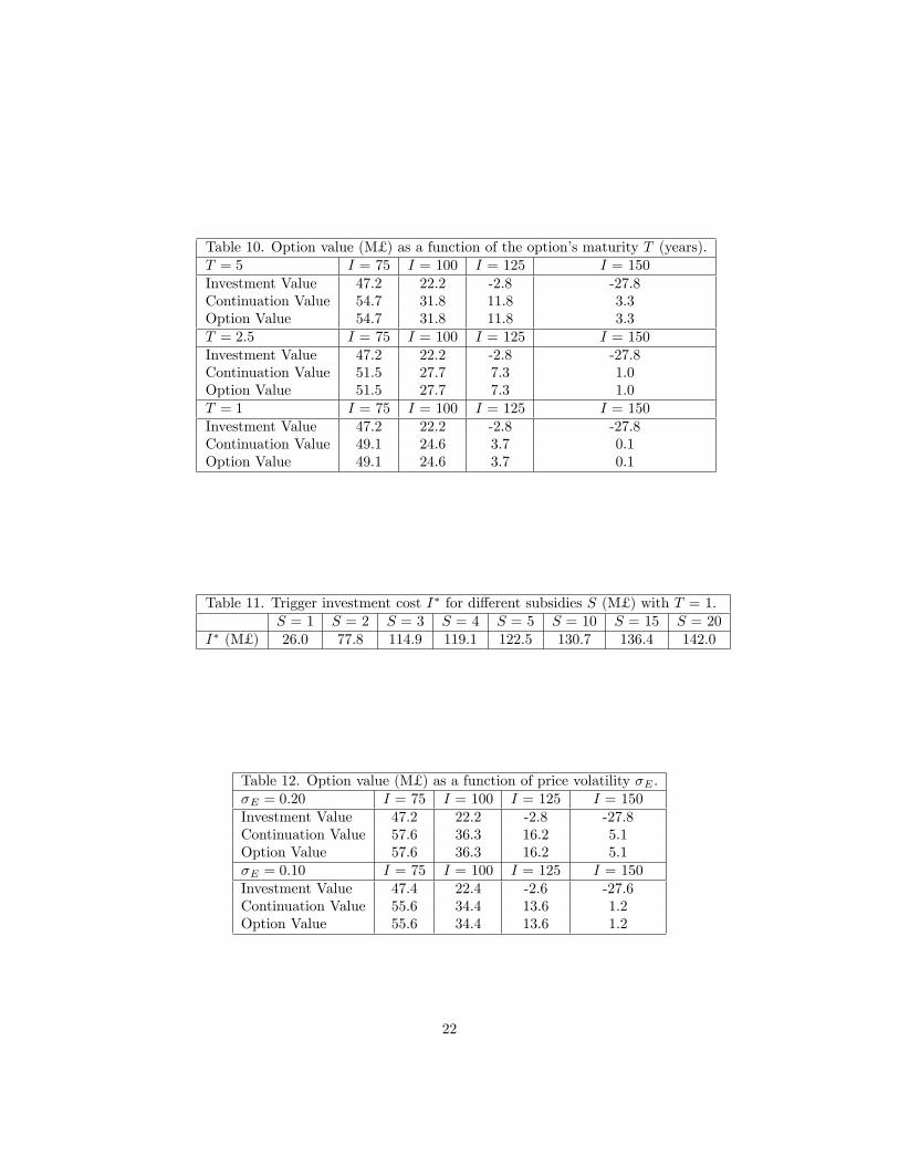
Table 10. Option value (M£ ) as a function of the option�s maturity T (years).T = 5 I = 75 I = 100 I = 125 I = 150Investment Value 47.2 22.2 -2.8 -27.8Continuation Value 54.7 31.8 11.8 3.3Option Value 54.7 31.8 11.8 3.3T = 2:5 I = 75 I = 100 I = 125 I = 150Investment Value 47.2 22.2 -2.8 -27.8Continuation Value 51.5 27.7 7.3 1.0Option Value 51.5 27.7 7.3 1.0T = 1 I = 75 I = 100 I = 125 I = 150Investment Value 47.2 22.2 -2.8 -27.8Continuation Value 49.1 24.6 3.7 0.1Option Value 49.1 24.6 3.7 0.1

Table 11. Trigger investment cost I� for di¤erent subsidies S (M£ ) with T = 1.S = 1 S = 2 S = 3 S = 4 S = 5 S = 10 S = 15 S = 20

I� (M£ ) 26.0 77.8 114.9 119.1 122.5 130.7 136.4 142.0

Table 12. Option value (M£ ) as a function of price volatility �E .�E = 0:20 I = 75 I = 100 I = 125 I = 150Investment Value 47.2 22.2 -2.8 -27.8Continuation Value 57.6 36.3 16.2 5.1Option Value 57.6 36.3 16.2 5.1�E = 0:10 I = 75 I = 100 I = 125 I = 150Investment Value 47.4 22.4 -2.6 -27.6Continuation Value 55.6 34.4 13.6 1.2Option Value 55.6 34.4 13.6 1.2

22

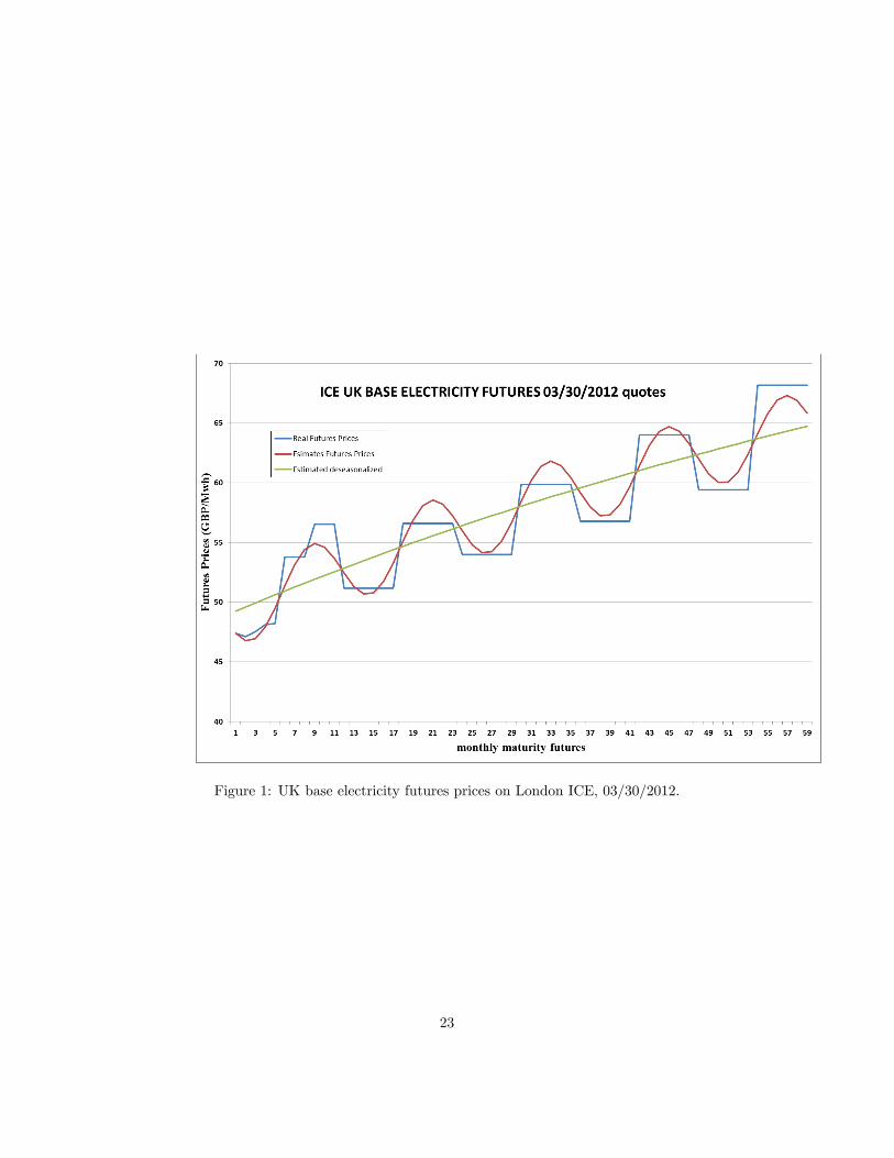
Figure 1: UK base electricity futures prices on London ICE, 03/30/2012.

23

Figure 2: Monthly load factor of UK wind farms 2006-10.

24

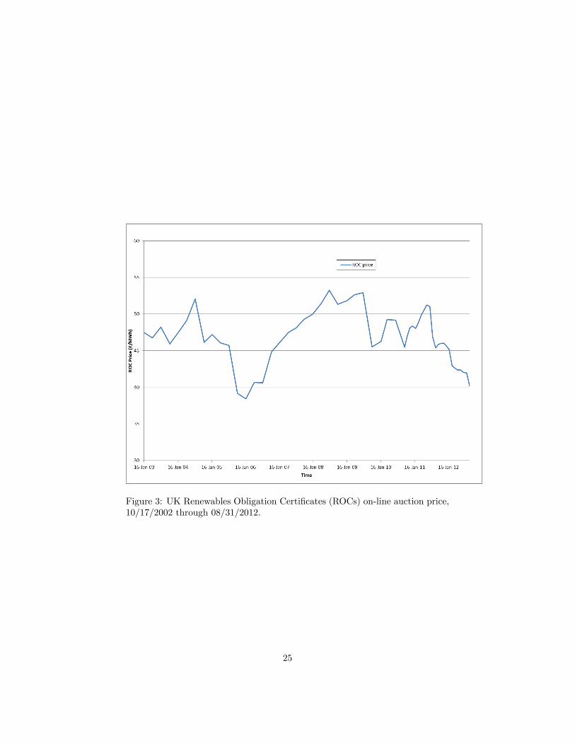
Figure 3: UK Renewables Obligation Certi�cates (ROCs) on-line auction price,10/17/2002 through 08/31/2012.

25