value-at-risk in portfolio optimization: properties and...
TRANSCRIPT

Value-at-Risk in Portfolio Optimization: Properties andComputational Approach∗
Alexei A. Gaivoronski∗ and Georg Pflug∗∗∗Department of Industrial Economics and Technology Management
NTNU - Norwegian University of Science and Technology
Alfred Getz vei 1, N-7049 Trondheim, Norway
[email protected]∗∗Department of Statistics, University of Vienna
Universitaetsstrasse 5, A-1010 Vienna, Austria
Abstract
The Value-at-Risk (V@R) is an important and widely used measure of the extent towhich a given portfolio is subject to risk inherent in financial markets. In this paper, wepresent a method of calculating the portfolio which gives the smallest V@R among those,which yield at least some specified expected return. Using this approach, the completemean-V@R efficient frontier may be calculated. The method is based on approximating thehistoric V@R by a smoothed V@R (SV@R) which filters out local irregularities. Moreover,we compare V@R as a risk measure to other well known measures of risk such as theConditional Value-at-Risk (CV@R) and the standard deviation.
It is shown that the resulting efficient frontiers are quite different. An investor, whowants to control his V@R should not look at portfolios lying on other than the V@R effi-cient frontier, although the calculation of this frontier is algorithmically more complex. Wesupport these findings by presenting results of a large scale experiment with a representativeselection of stock and bond indices from developed and emerging markets which involvedthe computation of many thousands of V@R-optimal portfolios.
1 Introduction
The Value-at-Risk (V@R) is an important measure of the exposure of a given portfolio of se-curities to different kinds of risk inherent in financial markets. By now, it became a tool forrisk management in financial industry (RiskMetricsTM 1995) and part of industrial regulatorymechanisms (Amendment to the Capital Accord to Incorporate Market Risks 1996). Considerable
∗Journal of Risk, Vol. 7, No. 2, pp. 1-31, Winter 2004-2005
1

amount of research was dedicated recently to development of methods of risk management basedon Value-at-Risk 1.
In this paper we focus on applications of the Value-at-Risk (V@R) concept in the contextof optimal portfolio selection. This is a relatively novel application of V@R as opposed toutilization of V@R for risk measurement purposes. One of the reasons is that V@R optimizationis inherently more difficult than – for example – variance optimization and efficient solutionalgorithms for this problem are lacking. The V@R optimization problem is nonconvex, mayexhibit many local minima and is of combinatorial character, i.e. exhibits exponential growthin computational complexity. The objective of this paper is to demonstrate how to solve V@Roptimization problems and to put V@R on equal footing with the variance as portfolio selectioncriterion. We present a smoothing algorithm, which allows to calculate optimal portfolios in theV@R sense accurately and in reasonable time.
Recently, the possibilities to utilize V@R and related measures like the Conditional Value-at-Risk (CV@R, see Uryasev & Rockafellar (1999)) as criteria for optimal portfolio selectionstarted to attract some attention. The relevant literature includes Basak & Shapiro (2001),Gaivoronski & Pflug (1999), Krokhmal, Uryasev & Palmquist (2001), Medova (1998), Uryasev& Rockafellar (1999) and sheds an interesting light on the properties of V@R-optimal portfolioswhile acknowledging considerable computational difficulties which we address in this paper.2
Another aim of this paper is to make computational comparisons of the properties of V@R,CV@R and standard deviation as risk measures in context of portfolio selection. In the centerof our approach is the comparison of efficient frontiers for different data sets, some of them ofconsiderable interest for institutional investors. This study can be seen as complementary tocomparison of theoretical properties as in Artzner, Delbaen, Eber & Heath (1999) or evaluationof risk measures from the utility theory standpoint as in Grootveld & Hallerbach (2000) andKaplanski & Kroll (2002). We argue that for an investor whose risk preferences are expressedin terms of Value-at-Risk it is important to consider this measure directly because other riskmeasures like standard deviation, or even the seemingly related CV@R may represent a poorsubstitute. Empirical comparisons of V@R and other risk measures from different angles can befound in Wu & Xiao (2002) and Pfingsten, Wagner & Wolferink (2004).
The rest of the paper is organized as follows. In section 2 we introduce the three risk-returnoptimization problems for standard deviation (or equivalently variance), V@R and CV@R anddiscuss their properties illustrating our points by numerical examples. We concentrate hereon empirical risk measures derived directly from historic data. In other words, our approachis based on historic simulation. The main finding is that historical V@R can be representedby a superposition of two components: one is relatively well behaved and the other is highlyirregular. This observation is exploited in section 3 where we introduce the smoothed Value-at-Risk (SV@R) which is an approximation of V@R, which extracts the global component of
1See e.g. Jorion (2001) and Duffie & Pan (1997) for surveys2V@R optimization can be considered as a stochastic programming (SP) problem of special type. It is related
to SP problems with probability constraints (Prekopa 1995). General references for stochastic programming mod-els and solution techniques are Birge & Louveaux (1997), Ermoliev & Wets (1988), Kall & Wallace (1994), Wets(1982) among others. Different applications of SP to optimal asset allocation were considered in Carino & Ziemba(1998), Consigli & Dempster (1998), Dembo & Rosen (1999), Dupacova, Bertocchi & Moriggia (1998), Gaivo-ronski & de Lange (2000), Gaivoronski & Stella (2000), Mulvey & Vladimirou (1992), Ogryczak & Ruszczynski(1999), Zenios (1993), fast computation of several mean-risk efficient portfolios was considered in Duarte (1999).
2

the V@R behavior and filters out the irregular local component. The mathematical details ofour SV@R construction are fairly involved and therefore we relegate them to Appendix. SV@Roptimization is much easier and can be performed by efficient nonlinear programming software.The optimal V@R values are recovered from the solution of SV@R optimization problem bya few inexpensive postprocessing steps. After developing V@R optimization tools3, we arein position to compute and compare mean-risk efficient frontiers for different risk measures insection 4. An important result of this comparison is that mean-V@R efficient frontier cannot beapproximated by efficient frontiers obtained for other risk measures, like the standard deviationor CV@R and therefore V@R-optimal portfolios should be considered directly. We provideadditional evidence in support for this recommendation in section 5, where results of a largescale experiment with a representative set of financial data are reported. The data set containsstock and bond indices for several developed and emerging markets and involved computation ofmore than 80000 V@R-optimal portfolios using the SV@R approximation. Both in sample andout of sample experiments confirm advantage of V@R-optimal portfolios in terms of controllingV@R.
2 Risk-return portfolio optimization
Consider a finite set of arbitrary financial assets i = 1, 2, . . . , n. Within a given observationperiod these assets generate returns
ξ = (ξ1, ξ2, . . . , ξn),
measured as the relative increase (or decrease) of the asset prices during the period under con-sideration. These returns are unknown at the time of portfolio allocation and are treated asrandom variables. The investor has a budget of 1 unit (without loss of generality). He/she maydecide on the positions
x = (x1, x2, . . . , xn)
in these assets, such that xi ≥ 0 (no short sales permitted) and∑n
i=1 xi = 1 (budget constraint).Using the vector 1l = (1, . . . , 1) of ones, we may write the budget constraint as xT 1l = 1. Thereturn of the portfolio at the end of the observation period is
W = xT ξ =n∑
i=1
xiξi.
It is a random variable with distribution function F , i.e. F (u) = P{W ≤ u} = P{xT ξ ≤ u}. Ofcourse, F depends on x. The expected return of portfolio x is
E(W ) = E(xT ξ) = xTE(ξ).
3More information about V@R optimization tools developed in this paper, distributable software and resultsof additional computations is found at http://websterii.iot.ntnu.no/users/alexeig/VaR/
3

Suppose that R is some risk measure, like V@R, CV@R or the standard deviation. For a givenminimal expected return µ, let us consider the solution of the following optimization problem:
minxR(xT ξ) (1)
xTE(ξ) ≥ µ
xT 1l = 1
x ≥ 0
The curve which represents the dependence of the optimal value of this problem on the parameterµ is the boundary of the feasible set of values of pairs (return, risk). A subset of this boundaryforms the R-efficient frontier and individual portfolios on this frontier are R-efficient portfolios.Essentially, this is a generalization of the classical concept of mean-variance efficient frontier dueto Markowitz (1952) for the case of an arbitrary risk measure R.
In this paper we are going to compare risk-return optimal portfolios obtained through solutionof (1) for the following risk measures.
1. The Value-at-Risk (V@R)
R(W ) = V@R(W ) = E(W )− Qα(W ) (2)
where Qα(W ) is the α−quantile of return:
Qα(W ) = inf{u : F (u) > α}.
The definition which we use describes the largest return underperformance relative to expectedportfolio return which is possible in 1−α cases of outcomes. We shall refer to 1−α as a confidencelevel4.
2. The Conditional Value-at-Risk (CV@R)
R(W ) = CV@R(W ) = E(W )− Cα(W ). (3)
where Cα(W ) is the expectation of return conditioned on not exceeding the α−quantile, or moreprecisely
Cα(W ) =P{W ≤ Qα(W )}
αE(W |W ≤ Qα(W )) +
(1− P{W ≤ Qα(W )}
α
)Qα(W ). (4)
Notice that Cα(W ) = E(W |W ≤ Qα(W )) in case that P{W ≤ Qα(W )} = α, e.g. if W has nopoint mass at Qα(W ).
Usually the values of α in these definitions are taken to be small, say, 0.05 or 0.01.
4Several slightly different definitions of V@Rcan be found in the literature. Other V@R definitions can berecovered easily from this. In the case of short observation period (few days) one often takes V@Rα(W ) ' −Qα(W ) since in this case E(W ) ' 0 for any reasonable portfolios. Our results are not influenced by difference inthese definitions.
4

3. The Standard deviation (StDev)
R(W ) = StDev(W ) =
√E (W−E(W ))> (W−E(W ))
2.1 Optimal portfolios based on historical or simulated data
In order to obtain risk-optimal portfolios through the solution of problem (1) we have essentiallytwo possibilities.
1. The parametric approach. It is assumed that the asset returns are governed by a givenparametric distribution with known parameters, for example normal or lognormal. Using thisknowledge one may obtain analytical expressions or algorithmic procedures for computation ofrisk measure R(xT ξ) and its other quantities necessary for optimization, like derivatives. This isquite possible to do when the risk measure is the standard deviation. In this case problem (1)is equivalent to a quadratic optimization problem for which efficient codes exist. Unfortunately,this approach becomes problematic for the case of V@Rand CV@Rbecause precise computationof these measures for continuously distributed returns may be very difficult unless the returndistribution is normal.
2. The sampling approach. It works directly with a finite sample ξ1, ξ2, . . . , ξN of returnobservations without assuming any specific distribution for returns. This sample can be actualhistoric data from which V@R or CV@R is computed through historic simulation or by para-metric Monte Carlo. We follow this approach here because it is computationally feasible forconsiderably larger class of risk-return optimization problems, especially in the case of V@R andCV@R. Besides, both V@R and CV@R are sensitive to the tail properties of distributions andmany parameterized families are notoriously bad in describing such properties of real data.
Using the three different risk measures V@R(W ), CV@R(W ) and StDev(W ) in (1), thesampling approach leads to quite differently structured optimization problems.
The StDev optimization problem is equivalent to the variance optimization problem, whichis a convex quadratic program:
minx≥0
xT
[1
N
N∑i=1
(ξi − e)(ξi − e)
]x (5)
xT e ≥ µ (6)
xT 1l = 1 (7)
where e = 1N
∑Ni=1 ξi is the average return vector.
The formulation of the sample CV@Roptimization problem requires more work. Observe thatfor any fixed portfolio x the value of Cα(W ) from (4) can be represented as the solution of thefollowing optimization problem (Uryasev & Rockafellar 1999):
Cα(W ) = − infa∈R{−a +
1
αEmax [W − a, 0]}. (8)
5

Given the relation (3) one may write the CV@R optimization problem as follows:
minx≥0,a
−a +1
αN
N∑i=1
max[a− xT ξi, 0]
with additional constraints (6),(7). Let us introduce here auxiliary variables z = (z1, .., zN) suchthat zi ≥ max[a− xT ξi, 0]. This yields the following large scale linear programming problem:
minx≥0,z≥0,a
−a +1
αN
N∑i=1
zi (9)
a− xT ξi − zi ≤ 0
with constraints (6),(7). Efficient commercial software exists for the solution of this problem.For the definition of the V@R optimization problem let us denote by mink
{u1, . . . , uN
}and
maxk{u1, . . . , uN
}the k-th smallest and the k-th largest among u1, . . . , uN . Then min1
{u1, . . . , uN
}and max1
{u1, . . . , uN
}will be the ordinary minimum and maximum. Besides,
min k{u1, . . . , uN
}= max N−k+1
{u1, . . . , uN
}, min k
{u1, . . . , uN
}= −max k
{−u1, . . . ,−uN}
.
In these notations the empirical α-quantile of the sample xT ξ1, . . . xT ξN is V (x) = min bαNc+1{xT ξ1, . . . xT ξN
}where bαNc is the largest integer not exceeding αN . The empirical V@R5 from definition (2) is
V@R(x) = xT e− min bαNc+1{xT ξ1, . . . xT ξN
}(10)
which yields the following V@Roptimization problem6.
minx∈X
−V (x) (11)
where
V (x) = min bαNc+1{xT ξ1, . . . , xT ξN
}
and
X = {x ≥ 0; xT e ≥ µ; xT 1l = 1}.
This problem is a nonconvex program which may have many local minima because the func-tion maxk of N linear functions is convex only for k = 1 when it coincides with ordinary maxi-mum. This makes it by far the most difficult problem to solve among the problems (5),(9),(11).While efficient commercial software based on several decades of algorithmic and theoretical re-search exists for solution of problems (5) and (9), the current situation with the problem (11)is the opposite one. Efficient general algorithms for minimization of functions defined throughmaxk are nonexistent. Our aim here is to exploit the structure of (11) and develop efficient
5When sample is drawn from historic prices this is called the historic V@R6We assumed here and in (9) that for the set of assets under consideration the less risky portfolios do not
yield superior average returns compared to more risky portfolios. Then the first term in (10) will not affect thesolution of risk-optimization problem (1) and can be dropped.
6

solution techniques specifically tailored for V@R optimization problem.
2.2 Properties of V@R and CV@R optimal portfolios
In this section we present an empirical study of the properties of historic V@R and CV@R asfunctions of portfolio composition using stock market data. Its purpose is to give a motivationfor the numerical approach of Section 3 for the solution of problem (11) without making anygeneral claims about the properties of portfolios of equities. Here and in the sections 3, 4 weutilized the same data set which was used in Cover (1991) and a number of other papers forevaluation of so-called universal portfolios. It contains more than 20 years of NYSE stock dailyreturns for representative set of 36 companies from different industry sectors starting from July3, 1962 to December 31, 1984. In all experiments reported here we used this data starting fromthe first day, July 3, 1962.
Typical patterns of V@Rdependence on portfolio composition are presented on Figure 1.Two portfolios were selected, say, x1 and x2, and the family of portfolios x(λ) was considered
which is defined by linear combination of these two portfolios:
x(λ) = λx1 + (1− λ)x2, 0 ≤ λ ≤ 1 (12)
Figure 1 shows sample V@R(thin line) and CV@R(thick line) of portfolio x(λ) as function of λ.The values of λ are shown on horizontal axis, while the vertical axis represents values of V@Rand CV@R measured in percentage points of initial portfolio value. These risk measures arecomputed using 500 observations over a 10 days period, with α = 0.05. Portfolio x1 contains onlyFord stock and portfolio x2 contains only Hewlett Packard stock. These and other experimentsprovide the following observations about the behavior of V@R.
1. The sample V@R is a very irregular function with multiple local minima and maximaevenly distributed in the function domain. The value of the local minima is in large majorityfar away from the globally minimal V@R value. We performed many experiments where thenumber of observations was increasing from 250 to 5000. They show that the number of localminima grows with the number of observations and sooner or later a portfolio where V@R attainsits locally minimal value can be found in the vicinity of almost every portfolio. Moreover, theV@R function is nondifferentiable in every local minimum. This means that a straightforwardapplication of standard techniques of nonlinear optimization to the solution of problem (11) isvery problematic. Usually such methods require differentiability of the objective function, whichis not the case here. Even if a method can overcome this obstacle, it still could find only a localminimum of the V@R function. This will not bring us any closer to the solution of (11) becausean arbitrary local minimum does not provide any information about the solution of the V@Roptimization problem.
2. The V@R function possesses a pronounced structure and is composed of two components.The first component exhibits the fairly regular global pattern with a unique global minimumand smooth behavior which in some cases is close to a convex function7. The second componentis responsible for the local behavior and has a highly irregular pattern which produces almost
7In some other examples its behavior did not seem to be convex, but it still had only a few local minima withvalues which are close to the global minimum, see thick line on Figure 2
7

0 0.1 0.2 0.3 0.4 0.5 0.6 0.7 0.8 0.9 16
6.5
7
7.5
8
8.5
9
9.5
10
Fraction of Ford stock in portfolio
VaR
, CV
aR (
%)
VaRCVaR
Figure 1: Properties of V@R and CV@R for Ford/HP portfolio
all local minima and nondifferentiability. This dissection into two components is crucial for ourapproach to the solution of the V@R optimization problem (11).
Before starting with dedicated techniques for optimizing V@R let us explore briefly an al-ternative approach: the substitution of V@R with some related risk measure which is easier tooptimize. If portfolios optimal for such alternative measure have V@R which is close to the op-timal V@R then there is no need to develop dedicated techniques for V@R. A natural candidatefor such substitution is CV@R which is the smallest convex majorant of V@R and which maybe optimized using the solution of linear program (9), a relatively simple issue. In order to getsome empirical evidence about the relation between CV@R and V@R optimal portfolios, weconducted a series of experiments with the same data set as before.
For each experiment a pair of stocks was selected and the set of portfolios defined by (12)was considered, where portfolios x1 and x2 consisted of pure stocks 1 and 2 respectively. Fromthis set we selected portfolios with minimal V@R and CV@R which are denoted by xV@R andxCV@R. This is a simple thing to do because we have one-dimensional optimization problem here.Suppose now that the V@R-optimal portfolio xV@R is substituted by the CV@R-optimal portfolioxCV@R. By doing so we make two kinds of substitution errors: we get a larger V@R(xCV@R) valueand a different value of portfolio return R(xCV@R). These errors are measured as follows:
EV@R =V@R(xCV@R)− V@R(xV@R)
V@R(xV@R)100%, ER =
R(xV@R)−R(xCV@R)
R(xV@R)100% (13)
Our experiments show that in some cases the CV@R-optimal portfolio approximates the V@R-optimal portfolio reasonably well. In other cases the CV@R-optimal portfolio is a poor substitutefor V@R-optimal portfolio because the substitution error is not much better compared to the
8

error of randomly selected portfolio. Some such cases are summarized in the Table 1. V@Rerrors for randomly selected portfolios formed by the stock pairs from this table are only 60-100% larger compared to the errors of CV@R-optimal portfolios. Differences in returns can bevery substantial and considerably different compositions of optimal portfolios may occur. Figure1 presents in more detail the case of Ford-Hewlett Packard portfolio from this table. Note thatCV@Ris a convex function in the portfolio shares, while V@Ris not, and they take their respectiveminima in considerably different regions.
Stocks V@R error EV@R Return error ER
Kodak-Merck 5.3 5.6General Electric-IBM 3.4 2.4Sears-Coca Cola 6.1 11.7Dupont-Exxon 6.0 -11.4P&G-GTE 8.1 -0.1Ford-HP 7.9 30.3GM-P&G 10.0 5.3
Table 1. Errors committed by substitution of V@R by CV@R, confidence level 0.95, 500observations over 10 days period, starting day July 3, 1962
This evidence motivates the development of dedicated techniques for the computation ofV@R optimal portfolios through the solution of problem (11). More evidence in this directionis presented in Sections 4,5 where respective efficient frontiers are compared.
3 Computation of V@R efficient portfolios using SV@R
The analysis of the previous section is the basis of our approach to the numerical solution of theV@R optimization problem (11) which consists of three steps.
1. Smooth out the local noisy component of the V@R function and extract the well behavedglobal component. This is the key feature of our approach. The result is the smoothed V@Rfunction (SV@R).
2. After this the problem (11) becomes treatable by standard off-shelf software developedfor solution of nonlinear programming problems. We want to utilize this software as much aspossible. The result is an approximate solution of the V@R optimization problem which in itselfwill be often sufficient for practical purposes.
3. Postprocessing of the approximate solution. This is an optional step where commercialoptimization software is used again.
1. Extracting the global behavior of the V@R function: SV@RIn principle, general approximation techniques, like spline approximation, can be used for
smoothing the V@R function. However, they require computational overhead which grows ex-ponentially with the dimension of the portfolio. This makes such approaches impractical becausethe approximating function is going to be computed repeatedly during the optimization process.For this reason, we had to develop the smoothing techniques which exploits the special structureof the V@R function.
Consider the sample quantile function V (x) from (11). It depends on the portfolio shares x,the observations of return ξ1, ..., ξN and the probability level α. This function is approximated
9

by the family of smoothed quantile functions V (ε, x) parameterized by smoothing parameter ε,ε > 0:
V (ε, x) =N∑
i=1
cεi(x)xT ξi. (14)
The coefficients cεi(x) in (14) satisfy the following conditions:
1. cεi(x) are twice continuously differentiable for all ε > 0.
2. cεi(x) → 0 as ε → 0 for every x and i for which V (x) 6= xT ξi.
3. cεi(x) → 1/N as ε →∞ for every x and i.
4.∑N
i=1 cεi(x) = 1.
Under these conditions V (ε, x) is twice continuously differentiable8 for all ε > 0. Anotherconsequence of conditions 1-4 is that V (ε, x) → V (x) as ε → 0 and
V (ε, x) → 1
N
N∑i=1
xT ξi
as ε → ∞ which is just the average return of portfolio x. Thus, we have the whole range ofapproximations from very precise approximations for small values of ε which, however, leaveuntouched the undesired properties of the original quantile function, to very well behaved, al-most linear approximations which, however, retain little information about the original quantilefunction. Therefore, the choice of smoothing parameter ε is governed by trade-off between twoconflicting objectives of having precise approximation and having smooth approximation with asfew local minima as possible.
A large family of possible selections for cεi(x) from (14) is described in Appendix (see (26)-
(27) and Theorem 2). Each specific expression for cεi(x) is defined by a function ϕε(z) of one
dimensional parameter z which provides a smooth approximation for the unit step function ϕ(z) :
ϕ(z) =
{1 if z ≤ 00 otherwise
Smooth approximants ϕε(z) of ϕ(z) are defined in (28). This choice is driven by computationalconsiderations. The resulting smoothed quantile function V (ε, x) requires a moderate compu-tational overhead compared with the original quantile function V (x). The overhead does notdepend on the number of positions in portfolio x and grows relatively slow with the number ofreturn observations N (see Theorem 5). Figure 2 shows a typical example of a smoothed quantilefunction for different values of the smoothing parameter ε.
These figures show – similarly to Figure 1 – the dependence of the quantile function V (x)(thick line) on the parameter λ which defines portfolio x(λ) as linear combination of portfolios x1
and x2 obtained according to (12). Portfolios x1 and x2 consisted of three stocks (Schlumberger,Morris, Commercial Metals) in the following proportion:
x1 = (0.69668, 0, 0.30332), x2 = (0, 0.64624, 0.35376)
8This property is important because V (ε, x) is going to be minimized by standard nonlinear programmingalgorithms, and they usually require that the objective function has this property.
10

0 0.1 0.2 0.3 0.4 0.5 0.6 0.7 0.8 0.9 11.5
1.6
1.7
1.8
1.9
2
2.1
2.2
2.3VaRSVaR, slight smoothingSVaR, more smoothing
Figure 2: The quantile and the smoothed quantile function for different values of the smoothingparameter ε
V@Rwas computed on the basis of 500 daily observations for confidence level 0.95. Thin lineson this figure represents smoothed quantile function computed for different values of smoothingparameter ε. The solid thin line shows the case of small value of smoothing parameter ε = 0.001.In this case V (ε, x) follows V (x) very well, although even in this case the smoothing managedto cut off many irrelevant local minima. The case of larger value of ε = 0.004 is represented bya solid dashed line. Here local noisy component of V (x) is filtered out completely and only theglobal well behaved component remains.
2. Minimizing SV@RfunctionEfficient nonlinear programming software present in the market can be used for finding V@R-
efficient portfolios by minimizing the [email protected]. PostprocessingThe result of the previous step is portfolio xSV@R which is either a global minimizer or a good
local minimizer of the smoothed V@R function. In most cases this will be enough for practicalpurposes. However, if one wish to improve on this, it can be done by local minimization ofthe V@R function taking as a starting point portfolio xSV@R. For this purpose we solved linearprogramming problem of small to medium size10 formulated below.
9We implemented SV@Rin MATLAB environment (The Mathworks Inc. 1984-2004) and used fmincon subrou-tine from MATLAB Optimization Toolbox for its minimization. Another option is to use nonlinear programmingsolvers available in GAMS environment (Brooke, Kendrick, Meeraus & Raman 1998) or in NAG library.
10This can be done very fast by current commercial codes. We have found that subroutine linprog fromMATLAB Optimization Toolbox is sufficient for this purpose. Again, solvers present in GAMS environmentpresent another good choice.
11

According to (11) there exists index j which depends on xSV@R such that V (x) = xTSV@Rξj and
inequalityxT
SV@Rξi ≤ xTSV@Rξj (15)
is satisfied for at least bαNc observations ξi, i 6= j. Let us denote by Λ an arbitrary set ofbαNc indices for which inequality (15) is satisfied. Then the solution of the following linearprogramming problem is a local minimum of the quantile function V (x) and provides bettervalue of V@R then xSV@R.
minx
xT ξj (16)
xT(ξi − ξj
) ≤ 0, i ∈ Λ (17)
xT(ξi − ξj
) ≥ 0, 1 ≤ i ≤ N, i /∈ Λ (18)
xT e ≥ µ (19)
xT 1l = 1, x ≥ 0 (20)
Our experience is that the improvement of the V@R value obtained through solution of thisproblem is relatively small11.
4 Comparison of efficient frontiers
Now we have in place all tools necessary for utilization of V@R as a criterion for optimalinvestment. This is done following the classical Markowitz-type approach (Markowitz 1952):V@R is minimized for different values of minimal return µ by solving the problem (11) and themean-V@R feasible set is constructed from which the mean-V@R efficient frontier is derived.After this an investor with specific risk preferences can choose the target value of V@R andselect portfolio on the efficient frontier that provides the best return for a given value of V@R.
But how such mean-V@R efficient frontier compares with classical mean-variance efficientfrontier? If the difference is small there is no point in abandoning classical mean-variance ap-proach in favor of V@R. In order to answer this question we conducted a series of studies withprice data of different instruments. Here we report results obtained with the same set of thestock market data which was used in the section 2.1 and present the results graphically. Resultsof extensive experiments with portfolios of stock and bond indices are presented in the section5. The purpose was to compare different mean-risk efficient frontiers obtained on the basis ofhistorical data by solution of problems (5),(9) and (11) for different values of return µ. Eachcomputation of efficient frontier involved 200-500 solutions of respective optimization problem.
Results of a typical experiment are presented on Figures 3,4 and 5.
11It is possible to go further and minimize (16) subject to constraints (17)-(20) with respect to both portfoliox and all pairs (j, Λ) where 1 ≤ j ≤ N and set Λ contains exactly bαNc elements among integers {1, ..., N} \ {j} .This is a difficult mixed integer programming problem and it is practically impossible to solve it to optimality forproblems of realistic dimension without having good information about the optimal solution. However, minimumof smoothed V@R function xSV@R provides just this information. In our experiments we have not used this ap-proach because minimization of SV@R together with postprocessing according to (16)-(20) gave very satisfactoryresults.
12

4.5 5 5.5 6 6.5 7 7.5 8 8.50.4
0.45
0.5
0.55
0.6
0.65
0.7
0.75
0.8
0.85
0.9
VaR (%)
retu
rn (
%)
mean−variancemean−CVaRmean−VaR
Figure 3: Boundary of mean-V@R feasible set and images of mean-CV@R boundary and mean-variance boundary
6 7 8 9 10 11 120.4
0.45
0.5
0.55
0.6
0.65
0.7
0.75
0.8
0.85
0.9
CVaR (%)
retu
rn (
%)
mean−variancemean−CVaRmean−VaR
Figure 4: Boundary of mean-CV@R feasible set and images of mean-V@R boundary and mean-variance boundary
13
3 3.5 4 4.5 5 5.5 6 6.50.4
0.45
0.5
0.55
0.6
0.65
0.7
0.75
0.8
0.85
0.9
standard deviation (%)
retu
rn (
%)
mean−variancemean−CVaRmean−VaR
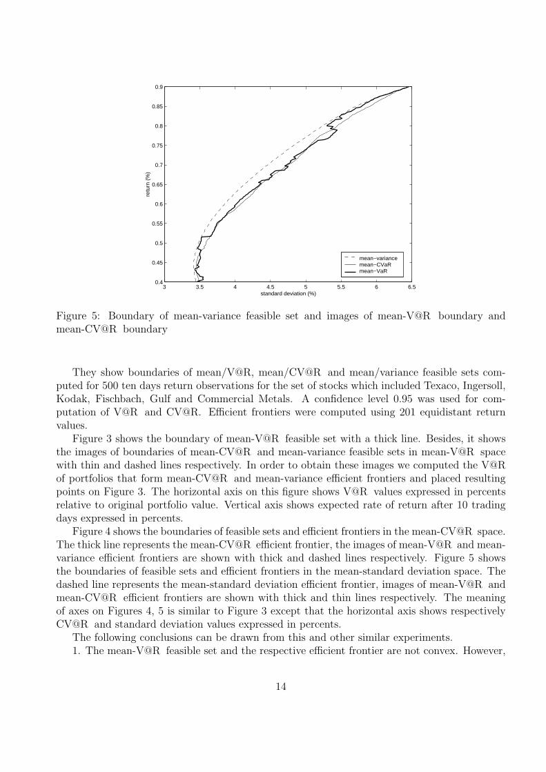
Figure 5: Boundary of mean-variance feasible set and images of mean-V@R boundary andmean-CV@R boundary
They show boundaries of mean/V@R, mean/CV@R and mean/variance feasible sets com-puted for 500 ten days return observations for the set of stocks which included Texaco, Ingersoll,Kodak, Fischbach, Gulf and Commercial Metals. A confidence level 0.95 was used for com-putation of V@R and CV@R. Efficient frontiers were computed using 201 equidistant returnvalues.
Figure 3 shows the boundary of mean-V@R feasible set with a thick line. Besides, it showsthe images of boundaries of mean-CV@R and mean-variance feasible sets in mean-V@R spacewith thin and dashed lines respectively. In order to obtain these images we computed the V@Rof portfolios that form mean-CV@R and mean-variance efficient frontiers and placed resultingpoints on Figure 3. The horizontal axis on this figure shows V@R values expressed in percentsrelative to original portfolio value. Vertical axis shows expected rate of return after 10 tradingdays expressed in percents.
Figure 4 shows the boundaries of feasible sets and efficient frontiers in the mean-CV@R space.The thick line represents the mean-CV@R efficient frontier, the images of mean-V@R and mean-variance efficient frontiers are shown with thick and dashed lines respectively. Figure 5 showsthe boundaries of feasible sets and efficient frontiers in the mean-standard deviation space. Thedashed line represents the mean-standard deviation efficient frontier, images of mean-V@R andmean-CV@R efficient frontiers are shown with thick and thin lines respectively. The meaningof axes on Figures 4, 5 is similar to Figure 3 except that the horizontal axis shows respectivelyCV@R and standard deviation values expressed in percents.
The following conclusions can be drawn from this and other similar experiments.1. The mean-V@R feasible set and the respective efficient frontier are not convex. However,
14

their distance from convex shape is relatively small and as the first approximation it can beconsidered ”almost” convex, especially if compared to irregular behavior of the V@R functionitself as shown on Figures 1-2.
2. V@Rdiffers substantially from both CV@R and variance because mean-V@R efficientportfolios may differ considerably from mean-CV@R or mean-variance efficient portfolios. Thedistance between V@R-efficient frontier and images of other frontiers can be considerably largerthan the distance between frontiers in mean-CV@Rspace or mean-variance space. Thus mean-CV@R and mean-variance efficient portfolios provide a poor approximation to mean-V@R effi-cient portfolios in mean-V@R space, while the opposite is not necessarily true. Besides, mean-CV@R efficient portfolios do not approximate mean-V@R efficient portfolios any better than themean-variance efficient portfolios do. Actually, in some cases mean-variance portfolios lie closerto mean-V@R portfolios than mean-CV@R portfolios, as Figure 3 suggests. Vice versa, mean-variance portfolios can approximate mean-CV@R portfolios better than mean-V@R portfoliosdo (see Figure 4).
3. As one can expect, all frontiers approximate each other fairly well for high risk portfoliosbecause for large return values all portfolios converge to portfolio consisting of only one assetwith largest return. For medium and low risk portfolios the difference between frontiers can besubstantial.
The experiments reported in this section represent a useful starting point for further studies.More evidence in the same direction is presented in the next section where we performed a muchlarger set of experiments.
5 Mean-risk optimal portfolios of stock and bond indices
The techniques developed in the previous sections allow to conduct experimental comparativestudies of properties of mean-risk portfolios for different sets of assets with the special emphasison mean-V@R efficient portfolios. In this section we report results of one such study whichinvolves a representative selection of broad asset classes of interest to an institutional investor.The objective of this study was twofold:
- Gain further insight into the properties of the proposed methodology for computing mean-V@R efficient portfolios with the help of smoothed V@R functions (SV@R).
- Evaluate experimentally the relative properties of mean-risk efficient portfolios. In particu-lar, we wanted to understand what advantage can give mean-V@R efficient portfolios to investorwhose risk control targets are formulated in terms of V@R compared to other mean-risk efficientportfolios.
5.1 Summary of results
The data set consisted of 16 market indices: 8 Morgan Stanley Equity Price Indices for USA, UK;Italy, Japan, Russia, Argentina, Brazil and Mexico and 8 J.P. Morgan Bond Indices (DevelopedMarkets and EMBI+ for Emerging Markets) for the same markets from January 19, 1999 to
15

May 15, 2002 expressed in US dollars12. This data set contained representative selection ofdeveloped and emerging stock and bond markets and allowed construction of a wide range ofportfolios from fairly safe to extremely risky. Moreover, it allowed to evaluate the performance ofmean-risk efficient portfolios in times of turbulent stock markets and extreme events in emergingmarkets, like Argentinian crisis of the second half of 2001. These indices were considered as thecomposite assets and it was assumed that an institutional investor can choose portfolios whichreproduce these indices.
Three types of experiments were performed with this data13.1. In sample experiments.(section 5.2). These involved computation of mean-risk efficient
frontiers from a given windows of historic data, exactly as it was done in section 4, around1100 of these frontiers were computed for each of the risk measures which required solution ofabout 250000 portfolio optimization problems (5), (9) and (11). Substantial differences betweendifferent frontiers were observed. In particular, the averaged maximal distance between mean-V@R efficient frontier and other frontiers exceeded 30%.
2. Out of sample experiments (section 5.3). Portfolios computed on step 1 were hold for afixed number of trading days following the time windows utilized for their computation (1-60days). Out of sample V@R was obtained from portfolio returns during the holding periods.V@R-optimal portfolios maintained advantage over the other mean-risk portfolios in terms ofV@R which in some cases arrived at the level of 10-17%.
3. Simulated management of investment fund 14. The same portfolios were used for simulatedmanagement of a hypothetical investment fund which for each trading day computes risk-efficientportfolios using newly arrived price information and use these portfolios for (possibly partial)rebalancing of its current portfolio. The V@R control advantage of V@R-optimal portfolios overother mean-risk portfolios arrived in some cases at the levels of 14-20%.
5.2 In sample experiments
We report here the results of experiment where the risk measures are computed using returnobservations over a short time horizon, for example over one day. The whole time horizont = 1, ..., T is divided into consecutive nonoverlapping periods of length n1. Asset returns arecomputed for all these periods which we call observation periods. Observations of return for n2
consecutive observation periods are used to compute statistical characteristics and risk measuresof return. This larger period of length n1n2 is called the sampling period. The time horizon t =1, ..., T contains T −n1n2 different sampling periods which start at times it = 1, ..., T −n1n2. Wecomputed boundaries of mean-V@R, mean-CV@R and mean-variance feasible sets by multiplesolving of respective risk minimization problems (11),(9) and (5) for all feasible sampling periods.
12We pruned days for which some of the emerging markets information was missing which left us with 829trading days of full price information.
13All experiments described in this section were performed on Dell Latitude 810 laptop with Windows 2000operation system equipped with Pentium III 1133 Mhz processor. Some critical parts of the Matlab code werereprogrammed in C in order to speed up execution times. More than 90% of the processing time was spent onsolving the mean-V@Roptimization problems (11). One solution of such problem took 4-5 seconds of CPU time.The parameters of the algorithm were fixed after few trial runs at the beginning and after that the computationof mean-risk optimal portfolios proceeded without any human intervention.
14Details of these experiments are available from the authors upon request
16

We report here results for T = 829, n1 = 1, n2 = 250 which yields 579 different mean-risk efficientfrontiers for each of the three risk measures15. That is, in this experiment we computed one daymean-risk efficient frontiers for 579 days from approximately one year of daily historic returndata immediately preceding each given day16.
The observed behavior of efficient frontiers was similar to one shown on Figures 3-5. Here wefocus on quantitative measures of difference between efficient frontiers.
1. Comparison of V@R of mean-V@R efficient portfolios and V@R of other mean-riskefficient portfolios.
In order to access numerically the gain which is obtained by substitution of mean-varianceor mean-CV@R efficient portfolios by mean-V@R efficient portfolios we computed the followingquantities:
EiV@R/CV@R =
V@R(xiCV@R)− V@R(xi
V@R)
V@R(xiV@R)
100%, EiV@R/StDev =
V@R(xiStDev)− V@R(xi
V@R)
V@R(xiV@R)
100%
Here the index i indexes all the risk minimization problems solved, i = 1 : 35459. Portfoliosxi
V@R, xiCV@R and xi
StDev denote obtained solutions of the i-th instance of the problems (11), (9) and(5) respectively. These measures express relative improvement of V@R estimates expressed inpercents. After that we computed the percentage of cases where improvement exceeded thresholdθ%. Results are shown in the table 2.
Threshold θ (%) -1 -0.1 0.1 1 2 5 10 20 30 40 50Ei
V@R/CV@R> θ (%) 99.95 99.79 93.77 90.32 85.90 70.99 43.69 13.56 4.72 0.88 0.15
EiV@R/StDev
> θ (%) 99.97 99.90 94.27 91.81 88.45 76.91 57.67 20.21 5.38 1.23 0.35
Table 2. Relative improvement of V@R by mean-V@R efficient portfolios.
We see that in the considerable fraction of cases V@R optimal portfolios constitute a sub-stantial improvement over CV@R and variance optimal portfolios as far as V@R is concerned.Indeed, improvement over 10% compared with variance optimal portfolios was obtained in around50% of cases in both experiments. Improvement over 30% still occurred in a few percent of caseswhile in some (rare) cases improvement exceeded 50%. Improvement over CV@R optimal port-folios is somewhat smaller but still substantial.
In a noticeable amount of cases which constituted around 6% the difference between differentmean-risk portfolios was within 0.1%. These cases correspond mostly to problems with either
15These frontiers were computed as follows. The equidistant grid of target returns µ0, ..., µk was set up andthe problems (5)-(11) were solved for all the values from this grid in the place of the constant µ in the respectivereturn constraints for which these problems were feasible. In this experiment we took µ0 = 0, µk = 0.8%, k =200, µi+1−µi = ∆µ = 0.004%. The total number of the grid points for which solution of problems (5)-(11) existedvaried with the position of the data window which supplied the return data and changed between 16 and 158.Totally, 35459 solutions of each of the problems (5)-(11) were computed.
16We also performed a different set of experiments with risk measures being computed for return observationsover larger time period of approximately one quarter (60 trading days). Observation periods overlapped in theseexperiments. These experiments showed very similar results and are not reported here. They are available fromthe authors upon request.
17

very high or very low values of return constraint where portfolios consisted of only few assetsand practically coincided.
Finally, in some extremely rare cases our techniques failed to find the global minimum of theV@R optimization problem and got struck in the local minimum which value exceeded the V@Rvalue of CV@R optimal or variance optimal portfolio. Still, the difference exceeded 1% only in1-2 cases from the total of 35459 cases reported in this table.
2. Comparison of efficient frontiers formed by mean-risk efficient portfolios.Here we focus on the whole efficient frontiers and characterize numerically the difference be-
tween given mean-V@R efficient frontier and images of mean-CV@Rand mean-variance efficientfrontiers into mean-V@R space. Similar characterization is given for mean-CV@Rand mean-variance efficient frontiers. In other words, we give a numeric expression to differences shown onFigures 3-5.
Let us denote by xiτV@R, xiτ
CV@R and xiτStDev the solutions of problems (11), (9) and (5) respectively
computed for value µi of target return and using historic price data from the time interval[τ −∆, τ ], we report here results with ∆ = n1n2 = 250 . Let us consider the following measuresof distance between mean-V@R efficient frontier and image of mean-CV@R efficient frontierinto mean-V@R space.
DτV@R/CV@R =
1
i+(τ)− i−(τ) + 1
i+(τ)∑
i=i−(τ)
V@R(xiτCV@R)− V@R(xiτ
V@R)
V@R(xiτV@R)
100%,
DτV@R/CV@R = max
i−(τ)≤i≤i+(τ)
V@R(xiτCV@R)− V@R(xiτ
V@R)
V@R(xiτV@R)
100%
where i−(τ) and i+(τ) are the indexes of the smallest and largest return µi from the target returngrid for which the solutions of problems (5)-(11) exist. The measure Dτ
V@R/CV@Ris the average
relative distance between frontiers while DτV@R/CV@R
is the maximal relative distance between
frontiers for a given time τ. We introduce distances DτV@R/StDev
, DτV@R/StDev
, DτCV@R/V@R
, DτCV@R/V@R
,
DτCV@R/StDev
, DτCV@R/StDev
, DτStDev/V@R
, DτStDev/V@R
, DτStDev/CV@R
, DτStDev/CV@R
in a similar manner. Thevalues of these distances are reported in Tables 3 and 4.
Distance DτV@R/CV@R
DτV@R/StDev
DτCV@R/V@R
DτCV@R/StDev
DτStDev/V@R
DτStDev/CV@R
Mean 7.98 9.76 5.25 1.87 3.19 1.20Max 18.75 22.89 11.51 6.216 8.475 3.740
Table 3. Distances between efficient frontiers measured by average relative difference
Distance DτV@R/CV@R
DτV@R/StDev
DτCV@R/V@R
DτCV@R/StDev
DτStDev/V@R
DτStDev/CV@R
Mean 30.81 30.44 18.80 7.29 10.85 6.40Max 59.92 64.85 40.99 14.82 14.82 15.86
Table 4. Distances between efficient frontiers measured by maximal relative difference
These tables show the average and maximal distances between efficient frontiers among 579triples of frontiers. Results give numeric confirmation to our assertion that V@R, CV@R andvariance can produce substantially different risk-optimal portfolios and different mean-risk ef-ficient frontiers. The average V@R difference between frontiers amounted to 8-10% and the
18
average maximal distance exceeded 30%. This means that at every time τ existed a target re-turn µ for which V@R of mean-CV@R and mean-variance efficient portfolios exceeded V@Rof V@R-optimal portfolio in average by more than 30%. The distances in mean-CV@R andmean-variance spaces were smaller, following the pattern present on Figures 3-5 and confirmingconclusions of section 4.
5.3 Out of sample experiments
Out of sample experiments permit to evaluate the potential of the mean-risk efficient portfoliosfor actual risk management purposes. Each of the portfolios computed during experimentsdescribed in the previous section is constructed by minimization of a given sample risk measureon the given sample interval [t − ∆, t] for a given values of t and ∆ and for a given value oftarget return µ. Therefore they possessed the target risk-return properties during this particularinterval. Suppose now that we simulate the holding of such portfolio for the time interval [t, t+τ ]of the length τ immediately succeeding the sample period for which portfolios were constructed.Will such portfolios exhibit desired risk-return properties also during this holding period? Forexample, will V@R-optimal portfolios still possess smaller V@R compared to CV@R-optimal orvariance-optimal portfolios? We show in this section that the answer to this question is positive.
The experiments consisted of the following steps.i. Fix the value of the target return µ, holding period τ and a risk measure among V@R,
CV@R and standard deviation.ii. For each t = ∆+1, ..., T −τ take mean-risk optimal portfolios computed for fixed values of
t and µ using return observations on the interval [t−∆, t]. Compute the return of these portfolioson the time interval [t, t+τ ]. This gives the set of return observations with T −τ−∆ elements17.
iii. Compute sample V@R for this set of return observations. Let us denote it by VaRV (µ, τ),VaRC(µ, τ) and VaRS(µ, τ) for the cases when the set of returns was generated correspondinglyby mean-V@R, mean-CV@R and mean-variance optimal portfolios. It characterizes the riskproperties of the whole set of mean-risk portfolios generated for all admissible times t and for agiven value of target return µ.
iv. Repeat steps i-iii for all three risk measures, all target returns µ = µi from the grid oftarget returns and all holding periods τ = 1, ...Tτ with Tτ = 60.
For each value µi of target return this experiment gives Tτ values of the relative V@RadvantageGiτ
V@R/CV@Rof V@R-optimal portfolios over CV@R-optimal portfolios
GiτV@R/CV@R =
V@RC(µi, τ)− V@RV (µi, τ)
V@RV (µi, τ)100% (21)
Averaging this measure over the set of holding periods τ gives the average V@R advantageGi
V@R/CV@Rof V@R-optimal portfolios over CV@R-optimal portfolios for fixed target return µi.The
measure of advantage GiV aR/StDev over variance-optimal portfolios is defined similarly. The results
of computation are presented in Table 5.
17provided that portfolio optimization problems (5)-(11) have solutions for this value of µ. In the case of τ = 60this yielded 519 return observations
19

max GiV@R/CV@R
average GiV@R/CV@R
max GiV@R/StDev
average GiV@R/StDev
9.8 4.5 7.1 1.6
Table 5. Out of sample advantage of V@R-optimal portfolios
The maximal and average values of measures GiV@R/CV@R
and GiV@R/StDev
presented in this tableare taken over the range of target returns which correspond to the range of yearly returns between5% and 25%. Thus, CV@R-optimal and variance-optimal portfolios do possess larger values ofout of sample V@R compared with V@R-optimal portfolios. Although difference averaged amongholding times and target returns is between 2-7%, for some values of returns it reaches 10% andin another set of experiments it arrived at 17%.
6 Summary
We studied here Value-at-Risk (V@R) in the context of V@R portfolio optimization for thepurpose of selection of mean-V@R efficient portfolios similar to the classical mean-varianceapproach. Important theme of this paper is comparison of V@R with other important riskmeasures from the optimization point of view, in particular with classical variance and morerecent conditional V@R(CV@R). This comparison is performed on computational plane usingthe stock market data and the representative selection of stock and bond indices from developedand emerging markets.
Our conclusion is that V@R is a substantially different risk measure and investor whichexpresses her risk preferences in terms of V@R should work with V@R directly in the contextof mean-risk trade-off. In particular, efficient frontiers constructed on the basis of the other riskmeasures can be a poor approximation for mean-V@R efficient frontier.
Moreover, we argue that computation of mean-V@R efficient portfolios based on historicdata is a feasible task, despite the fact that V@R optimization is more difficult than varianceoptimization or CV@R optimization. For this purpose we developed a set of V@R optimizationtools centered around the notion of smoothed V@R(SV@R) which filters out nonsmooth irregularlocal behavior of historic V@R. Effectiveness of SV@R approach to V@R optimization wasconfirmed during experiments reported in this paper which involved computation of more than80000 V@R-optimal portfolios.
7 Acknowledgment
We are grateful to the editor Professor Jorion and the anonymous referee for useful commentswhich contributed to improvement of the quality of exposition. Besides, we express our gratitudeto Dr. Giorgio Consigli who supplied us with financial data utilized for experiments in section 5.
8 Appendix: construction of SV@R
Here we provide mathematical details about the smoothing technique which was used in sections3-5 for computing of V@Refficient portfolios.
20

Let us consider a finite collection of functions fi(x), i = 1, ..., N defined on some set X ⊆ Rn.Let us fix k, 0 ≤ k ≤ N − 1 and define function
F (k, x) = maxi
k+1fi(x) (22)
which is equal to the k + 1−th largest from these functions. In other words, there exists someindex j = j(x) such that F (k, x) = fj(x) and inequality fj(x) ≤ fi(x) is satisfied for at least kfunctions fi(x), i 6= j while inequality fj(x) ≥ fi(x) is satisfied for at least N − k − 1 functionsfi(x), i 6= j.
Taking fi(x) = xT ξi we obtain that the minimization of F (k, x) in this case is the same assolution of (11). The function F (k, x) is nondifferentiable for all k even if functions fi(x) arearbitrarily smooth. Suppose that fi(x) are twice continuously differentiable. Our objective is toconstruct an approximation Fε(k, x) which depends on parameter ε such that
1. Fε(k, x) is twice continuously differentiable for all ε > 0;2. Fε(k, x) → F (k, x) as ε → 0.One possible way to obtain such approximation is a straightforward utilization of general
approximation techniques, like spline approximation. However, this approach is impracticalbecause it leads to exponential increase in computational complexity with respect to dimensionof x. We develop here another approach which exploits specific structure of the function F (k, x)and results in computational requirements which do not depend on dimension of x once values offi(x) are computed. For example, if fi(x) = xT ξi then the total computational requirements forcomputing Fε(k, x) at one point grow linearly with dimension of x. Our approximation is basedon the representation of the function F (k, x) as a linear combination of the composite functionsfi(x) where coefficients in the linear combination depend on x:
F (k, x) =N∑
i=1
ci(x)fi(x) (23)
In order to derive expressions for coefficients ci(x) we need the following notations:M i - set of all integers from 1 to N except i: M i = {1, 2, ..., N} \ {i} ;Λi
k - an arbitrary subset of M i which contains exactly k elements;X (Λi
k) - subset of Rn associated with set Λik as follows:
X(Λi
k
)=
{x : fi(x) ≤ fj(x) for j ∈ Λi
k, fi(x) ≥ fj(x) for j ∈ M i \ Λik
}
Θik - the family of all different sets Λi
k;IA - the indicator function of set A, i.e. IA = 1 if x ∈ A and IA = 0 otherwise. In order to
simplify notations we shall omit the dependence of IA on x where it will not cause confusion.The following lemma gives the required representation of function F (k, x).
Lemma 1 Suppose that F (k, x) is defined by (22). Then
F (k, x) =1
C(x)
N∑i=1
ci(x)fi(x), (24)
21

where
ci(x) =∑
Λik∈Θi
k
IX(Λik)
, C(x) =N∑
i=1
ci(x) (25)
Proof.Suppose that F (k, x) = fr(x). We are going to prove that also the right hand side of (24)
equals fr(x) provided coefficients ci(x) are selected according to (25).Let us consider an arbitrary i for which fi(x) > fr(x). Then inequality fi(x) ≥ fj(x) is
satisfied for at least N−k−1 functions fj(x) due to definition of function F (k, x). Consequently,inequality fi(x) ≤ fj(x) is satisfied for k1 < k functions fj(x) because from k1 = k would followfi(x) = fr(x). This means that x /∈ X (Λi
k) for arbitrary Λik because due to definition of set X (Λi
k)we have fi(x) ≤ fj(x) for at least k functions fj(x). Therefore IX(Λi
k)= 0 for arbitrary Λi
k and,
consequently, ci(x) = 0. By similar argument we obtain ci(x) = 0 also when fi(x) > fr(x). Thus,ci(x) can differ from zero only if fi(x) = fr(x). Therefore
1
C(x)
N∑i=1
ci(x)fi(x) = fr(x)1
C(x)
N∑i=1
ci(x) = fr(x)
due to (25). The proof is completed.¤We are ready now to formulate our main approximation result which defines a family of
smooth approximations of function F (k, x). It is presented in the following theorem.
Theorem 2 Suppose that fi(x) are twice continuously differentiable and ϕε(z) is an arbitraryfunction defined for z ∈ R1 and ε ≥ 0 such that
1. ϕε(z) is twice continuously differentiable for ε > 0.2. ϕε(z) → 1 as ε → 0 for any fixed z ≤ 0.3. ϕε(z) → 0 as ε → 0 for any fixed z > 0.4. ϕε(z) ≥ 0 for all ε ≥ 0, z and ϕε(z) ≥ κ0 for some κ0 > 0 and all ε ≥ 0, z ≤ 0.Then the function Fε(k, x) defined as follows:
Fε(k, x) =1
Cε(x)
N∑i=1
cεi(x)fi(x), (26)
wherecεi(x) =
∑
Λik∈Θi
k
∏
j∈Λik
ϕε
(∆x
ij
) ∏
j∈M i\Λik
ϕε
(−∆xij
), (27)
∆xij = fi(x)− fj(x), Cε(x) =
N∑i=1
cεi(x)
is twice continuously differentiable for all ε > 0 and such that Fε(k, x) → F (k, x) as ε → 0 forany fixed x.
Proof.
22

Let us fix x and suppose that r is such that F (k, x) = fr(x). Then from (22) follows thatthere exists set Λr
k ∈ Θrk such that fr(x) − fj(x) ≤ 0 for j ∈ Λr
k and fj(x) − fr(x) ≥ 0 forj ∈ M r \ Λr
k. Therefore due to condition 4 we have:
Cε(x) ≥ cεr(x) ≥
∏
j∈Λik
ϕε
(∆x
ij
) ∏
j∈M i\Λik
ϕε
(−∆xij
) ≥ κN−10 > 0
where the last estimate does not depend on x. This together with differentiability properties offi(x) and ϕε(z) yield existence and continuity of gradient and Hessian of Fε(k, x) for arbitrary xand ε > 0.
Observe now that ϕε(fi(x) − fj(x)) → I{fi(x)≤fj(x)} and ϕε(fj(x) − fi(x)) → I{fi(x)≥fj(x)} forarbitrary x and ε → 0 due to conditions 2,3. Therefore
∏
j∈Λik
ϕε
(∆x
ij
) ∏
j∈M i\Λik
ϕε
(−∆xij
) →∏
j∈Λik
I{fi(x)≤fj(x)}∏
j∈M i\Λik
I{fi(x)≥fj(x)} = IX(Λik)
which together with Lemma 1 yields cεi(x) → ci(x), Cε(x) → C(x) and finally Fε(k, x) → F (k, x)
for ε → 0 and arbitrary x. The proof is completed. ¤By selecting a family of functions ϕε(z), specific smooth approximation of the nondifferen-
tiable function F (k, x) can be obtained. Under additional technical assumptions this approxi-mation will converge uniformly to the original function. The selection of ϕε(z) should take intoaccount computational considerations. For general functions ϕε(z) the computation of cε
i(x) from(27) can be a difficult task because the number of terms in the sum from (27) grows exponen-tially with the number of observations N , more precisely it equals (N − 1)!/k! (N − k − 1)!. Thenumber of nonzero terms can be drastically reduced by special selection of function family ϕε(z),namely by considering only functions with the property ϕε(z) = 0 if z > ε. The simplest suchfunction that satisfies conditions of Theorem 2 is the cubic spline:
ϕε(z) =
1 if z ≤ 01− 16
3ε3z3 if 0 ≤ z ≤ ε
456
+ 2εz − 8
ε2z2 + 16
3ε3z3 if ε
4≤ z ≤ 3ε
4163− 16
εz + 16
ε2z2 − 16
3ε3z3 if 3ε
4≤ z ≤ ε
0 if z ≥ ε
(28)
The benefit of using such functions becomes clear from the following lemmas.
Lemma 3 Suppose that in addition to the conditions of Theorem 2 the function ϕε(z) is suchthat ϕε(z) = 0 if z > ε. Then the approximation function Fε(k, x) can be equivalently representedas follows:
Fε(k, x) =1
Cε(x)
∑
i:|F (k,x)−fi(x)|≤ε
cεi(x)fi(x) (29)
Proof.It is enough to prove that cε
i(x) = 0 if |F (k, x)− fi(x)| > ε. Let us fix i and consider the casewhen fi(x)− F (k, x) > ε. Let us select an arbitrary set of indices Λi
k ∈ Θik. Suppose that q ∈ Λi
k
23

and fq(x) = minj∈Λikfq(x). Then fq(x) ≤ F (k, x) due to definition of F (k, x). Therefore
fi(x)− fq(x) ≥ fi(x)− F (k, x) > ε
and, consequently, ϕε(fi(x)− fj(x)) = 0. Since Λik is arbitrary this means that every term in the
sum (27) which defines cεi(x) equals zero and cε
i(x) = 0. The case when F (k, x) − fi(x) > ε istreated similarly. ¤
Thus in order to compute Fε(k, x) it is enough to consider only those functions fi(x) forwhich |F (k, x)− fi(x)| ≤ ε which reduces considerably computational effort. Even though thisapproach makes possible to compute the values of Fε(k, x) for large N , still considerable care isneeded in implementation of (26)-(27) taking into account that Fε(k, x) is going to be computedmany times during optimization process. Let us derive equivalent expression for coefficientscεi(x), keeping in mind computational requirements. We shall consider the case when ϕε(z) = 1
if z ≤ 0 similar to (28).
Lemma 4 Suppose that in addition to conditions of Lemma 3 function ϕε(z) is such that ϕε(z) =1 if z ≤ 0. Then coefficients cε
i(x) from (27) can be represented equivalently as follows:
cεi(x) =
∑
q,r: q−r=k−ki−
b−q b+r (30)
b−q =∑
Λq⊆Λiε−
∏j∈Λq
ϕε
(∆x
ij
), b+
r =∑
Λr⊆ Λiε+
∏j∈Λr
ϕε
(−∆xij
)(31)
where Λr and Λq are arbitrary sets consisting of r and q elements respectively,
Λiε− =
{j : 0 < fj(x)− fi(x) ≤ ε, j ∈ M i
}, Λi
ε+ ={j : 0 ≤ fi(x)− fj(x) ≤ ε, j ∈ M i
}
and ki− is the number of elements in set Λi
ε−.
Proof.Let us fix x, select i and denote by Λi
− the set of all indices j = 1, ..., N such that fi(x) < fj(x).Suppose that ki is the number of elements in this set. Observe that an arbitrary set Λi
k ∈ Θik
can be represented as follows:
Λik =
(Λi− \ Λr
) ∪ Λq, M i \ Λik =
((M i \ Λi
−) \ Λq
) ∪ Λr
where Λr and Λq are arbitrary sets containing r and q elements respectively and such that
Λr ⊆ Λi−, Λq ⊆ M i \ Λi
−, ki + q − r = k
Since ϕε
(∆x
ij
)= 1 if j ∈ Λi
− \ Λr and ϕε
(−∆xij
)= 1 if j ∈ M i \ Λi
− \ Λq we can transform
24

expression (27) for coefficient cεi(x) as follows:
cεi(x) =
∑
Λr⊆Λi−
Λq⊆M i\Λi−
ki+q−r=k
∏j∈Λq
ϕε
(∆x
ij
) ∏j∈Λr
ϕε
(−∆xij
)
=∑
q,r: q−r=k−ki
∑
Λq⊆Λi−
∏j∈Λq
ϕε
(∆x
ij
)
∑
Λr⊆M i\Λi−
∏j∈Λr
ϕε
(−∆xij
)
Assertion of lemma is obtained from the last expression repeating the argument of Lemma 3which leads to substitution of Λi
− by Λiε−, M i \ Λi
− by Λiε+ and ki by ki
−. ¤Expressions (30),(31) allow efficient computation of coefficients cε
i(x) because b−q and b+r can
be computed recursively. Indeed, suppose that s ∈ Λiε−. Then
b−q = ϕε (∆xiv)
∑
Λq−1⊆Λiε−\{s}
∏j∈Λq−1
ϕε
(∆x
ij
)+
∑
Λq⊆Λiε−\{s}
∏j∈Λq
ϕε
(∆x
ij
)
The following algorithm utilizes the last expression in order to compute b−q for all q = 1, ..., qmax,qmax ≤ ki
−.
Algorithm 1.
1. Initialization. Select an arbitrary ordering j1, ..., jki−
of elements of set Λiε− and denote
ds = ϕε
(∆x
ijs
), s = 1, ..., ki
−. Take es = 1, s = 1 : ki− + 1.
2. Computation of b−q . Starting from q = 1 perform consecutively for each q = 1, ..., qmax :2a. Starting from s = q compute consecutively for each s = q, ..., ki
− :- Take a = dses if s = q and a = dses + a if s > q.- Take es = a if s > q.- Take a = a if s ≥ q.2b. Take b−q = a.The important question is how much additional computational work is needed in order to
compute Fε(k, x) compared to computation of F (k, x). Preliminary analysis of expressions (26)-(27) is not encouraging because the number of arithmetic operations necessary for straightforwardimplementation of (27) grows exponentially with the number of functions N . This will makethe computation of Fε(k, x) problematic even for moderate values of N. However, more refinedanalysis based on Lemma 4 and Algorithm 1 shows that in reality overhead grows relatively slowwhich makes computation of Fε(k, x) an easy task even for large N.
In order to make this statement precise we need to define exactly what we mean by com-putational overhead. For the purposes of the present discussion we shall measure overhead in anumber of arithmetic operations required for computation of Fε(k, x) after functions fi(x) arealready computed. We do not consider comparisons and memory management operations, buttheir inclusion will not lead to qualitatively different results. Overhead estimate is contained inthe following theorem.
25

Theorem 5 Suppose that ϕε(z) is computed according to (28). Then there exists an algorithmfor which the number S of additional arithmetic operations necessary for computation of Fε(k, x)for any fixed k, ε and x can be estimated as follows:
S ≤ (1 + ρN) N3 (32)
where N is the number of functions fi(x), ρN → 0 as N →∞, ρN ≤ 15 and ρN does not dependon dimension of vector x.
Proof.The proof is based on estimation of the number of arithmetic operations required by Algorithm
1 and implementation of expressions (29)-(31). Let us denote by ki+ the number of elements in
set Λiε+ and by k0 the number of elements in set Λk
ε ,
Λkε = {i : |F (k, x)− fi(x)| ≤ ε} .
Computation of all ds requires ki− subtractions in order to get ∆x
ijsand another at most 9ki
−operations in order to compute ϕε
(∆x
ijs
)if expression (28) is used. Step 2 of Algorithm 1 requires
ki−(ki
−+1)/2 multiplications and(ki−)2
/2 additions to compute all b−q for q = 1, ..., ki−. The same
algorithm can be used for computing of coefficients b+r . Computation of sum in (30) requires at
most 2 min{ki−, ki
+
}operations. Therefore we have the following estimate for the total amount
Si of arithmetic operations required for computation of cεi(x) for arbitrary fixed i:
Si ≤ ki−(ki
− + 1) + ki+(ki
+ + 1) + 2 min{ki−, ki
+
}+ 10ki
− + 10ki+ ≤
(ki−)2
+(ki
+
)2+ 12
(ki− + ki
+
).
The last inequality yieldsSi ≤ N2 + 12N
because ki− + ki
+ ≤ N. After all cεi(x) and fi(x) are computed it is required another 3k0 − 1
operations in order to compute Fε(k, x) from (29). Therefore the following estimate for S holds:
S ≤ k0
(N2 + 12N
)+ 3k0 − 1 ≤ N3 + 12N2 + 3N
which completes the proof. ¤In reality overhead will be much smaller than (32) because for small and moderate ε we have
ki− ¿ N, ki
+ ¿ N, k0 ¿ N. Estimates similar to (32) hold also for other functions ϕε(z) whichsatisfy conditions of Lemma 4.
Algorithm 1 and (29)-(31) were implemented as Matlab M-files and were used as the integralpart of environment for optimization of nonconvex nonsmooth functions F (k, x) by methods ofnonlinear programming designed for twice continuously differentiable functions.
References
Amendment to the Capital Accord to Incorporate Market Risks (1996), Bank for InternationalSettlements.
26

Artzner, P., Delbaen, F., Eber, J.-M. & Heath, D. (1999), Coherent measures of risk, Mathemat-ical Finance 9, 203 – 228.
Basak, S. & Shapiro, A. (2001), Value-at-risk based risk management: Optimal policies and assetprices, Rev. Financ. Stud. 14, 371–405.
Birge, J. R. & Louveaux, F. (1997), Introduction to Stochastic Programming, Springer, NewYork.
Brooke, A., Kendrick, D., Meeraus, A. & Raman, R. (1998), GAMS, A User’s Guide, GAMSDevelopment Corporation.
Carino, D. R. & Ziemba, W. T. (1998), Formulation of the Russell-Yasuda-Kasai financial plan-ning model, Operations Research 46(4), 433–449.
Consigli, G. & Dempster, M. (1998), Dynamic stochastic programming for asset-liability man-agement, Annals of Oper. Res. 81, 131–161.
Cover, T. M. (1991), Universal portfolios, Mathematical Finance 1(1), 1–29.
Dembo, R. & Rosen, D. (1999), The practice of portfolio replication. A practical overview offorward and inverse problems, Annals of Operations Research 85, 267–284.
Duarte, A. M. (1999), Fast computation of efficient portfolios, Journal of Risk 1(4), 1–24.
Duffie, D. & Pan, J. (1997), An overview of value at risk, Journal of Derivatives 4, 7–49.
Dupacova, J., Bertocchi, M. & Moriggia, V. (1998), Postoptimality for scenario based finan-cial planning models with an application to bond portfolio management, in W. Ziemba &J. Mulvey, eds, ‘Worldwide Asset and Liability Management’, Cambridge University Press,pp. 263–285.
Ermoliev, Y. & Wets, R. J.-B., eds (1988), Numerical Techniques for Stochastic Optimization,Springer Verlag, Berlin.
Gaivoronski, A. A. & de Lange, P. E. (2000), An asset liability management model for casu-alty insurers: Complexity reduction vs. parametrized decision rules, Annals of OperationsResearch 99, 227–250.
Gaivoronski, A. A. & Pflug, G. (1999), Finding optimal portfolios with constraints on Value-at-Risk, in B. Green, ed., ‘Proceedings of the Third International Stockholm Seminar on RiskBehaviour and Risk Management’, Stockholm University.
Gaivoronski, A. A. & Stella, F. (2000), Stochastic nonstationary optimization for finding univer-sal portfolios, Annals of Operations Research 100, 165–188.
Grootveld, H. & Hallerbach, W. G. (2000), Upgrading Value-at-Risk from diagnostic metric todecision variable: A wise thing to do? Working Paper, Erasmus University Rotterdam.
27

Jorion, P. (2001), Value at Risk: The New Benchmark for Managing Financial Risk, second edn,McGraw- Hill, New York.
Kall, P. & Wallace, S. (1994), Stochastic Programming, John Wiley and Sons, New York.
Kaplanski, G. & Kroll, Y. (2002), VAR risk measures vs traditional risk measures: An analysisand survey, Journal of Risk 4(3), 1–28.
Krokhmal, P., Uryasev, S. & Palmquist, J. (2001), Portfolio optimization with conditional value-at-risk objective and constraints, Journal of Risk 4(2), 43–68.
Markowitz, H. (1952), Portfolio selection, Journal of Finance 8, 77–91.
Medova, E. (1998), VAR methodology and the limitation of catastrophic or unquantifiablerisk. VII International Conference on Stochastic Programming, The University of BritishColumbia, Vancouver, Canada.
Mulvey, J. M. & Vladimirou, H. (1992), Stochastic network programming for financial planningproblems, Management Science 38(11), 1642–1664.
Ogryczak, W. & Ruszczynski, A. (1999), From stochastic dominance to mean-risk models: Semi-deviations as risk measures, European Journal of Operational Research 116, 33–50.
Pfingsten, A., Wagner, P. & Wolferink, C. (2004), An empirical investigation of the rank corre-lation between different risk measures, Journal of Risk 6(4), 55–74.
Prekopa, A. (1995), Stochastic Programming, Kluwer Academic Publishers.
RiskMetricsTM (1995), third edition, J.P. Morgan.
The Mathworks Inc. (1984-2004), Matlab 7.0, The MathWorks Inc.
Uryasev, S. & Rockafellar, R. (1999), Optimization of conditional value-at-risk, Technical Report99-4, ISE Dept. Univeristy of Florida.
Wets, R.-B. (1982), Stochastic programming: Solution techniques and approximation schemes,in A.Bachem, M.Groetshel & B.Korte, eds, ‘Mathematical Programming: The State of theArt’, Springer Verlag, Berlin.
Wu, G. & Xiao, Z. (2002), An analysis of risk measures, Journal of Risk 4(4), 53–75.
Zenios, S. A. (1993), A model for portfolio management with mortgage-backed securities, Ann.Oper. Res. 43, 337–356.
28