Value of a Limited Number of Discharge Observationsfor Improving Regionalization: A Large‐SampleStudy Across the United StatesS. Pool1 , D. Viviroli1 , and J. Seibert1,2

1Department of Geography, University of Zurich, Zurich, Switzerland, 2Department of Aquatic Sciences and Assessment,Swedish University of Agricultural Sciences, Uppsala, Sweden

Abstract Even in regions considered as densely monitored, most catchments are actually ungauged.Prediction of discharge in ungauged catchments commonly relies on parameter regionalization. Whileungauged catchments lack continuous discharge time series, a limited number of observations could still becollected within short field campaigns. Here we analyze the value of such observations for improvingparameter regionalization in otherwise ungauged catchments. More specifically, we propose an ensemblemodeling approach, where discharge predictions from regionalization with multiple donor catchments areweighted based on the fit between predicted and observed discharge on the dates of the availableobservations. It was assumed that a total of 3 to 24 observations from a single hydrological year wereavailable as an additional source of information for regionalization. This informed regionalization approachwas tested with discharge observations from 10 different hydrological years in a leave‐one‐out crossvalidation scheme on 579 catchments in the United States using the HBV runoff model. Dischargeobservations helped to improve the regionalization in up to 94% of the study catchments in 8 out of 10discharge sampling years. Sampling years characterized by exceptionally high peak discharge, or highannual or winter precipitation were less informative for regionalization. In the least informative years,model efficiency increased with an increasing number of observations. In contrast, in the most informativesampling year, 3 discharge observations provided as much information for regionalization as 24 dischargeobservations. Overall, discharge observations were most effective in informing regionalization in aridcatchments, snow‐dominated catchments, and winter‐precipitation‐dominated catchments.

1. Introduction

Continuous discharge time series are fundamental for many water management decisions in a river basin.However, even in regions considered as densely monitored, a considerable fraction of catchments areungauged or poorly gauged, that is, have no or only limited discharge data. Estimates of continuousdischarge time series in such catchments are often based on runoff models, which contain of a number oftuneable parameters that are typically derived from calibration against observed discharge. Determiningthese model parameters for data scarce catchments is one of the major challenges in hydrology(Hrachowitz et al., 2013).

In the absence of discharge data, model parameters can be estimated using regionalization methods,whereby hydrologic information is transferred from gauged to ungauged locations (Blöschl & Sivapalan,1995). Regionalization is a long‐standing research question in hydrology and has received special attentiondue to the PUB (Prediction in Ungauged Basins) initiative (Sivapalan et al., 2003). There are a great numberof regionalization approaches that have been proposed (for reviews see, e.g., He et al., 2011; Parajka et al.,2013; Razavi & Coulibaly, 2013). Although the most suitable regionalization approach is likely site specific(He et al., 2011; Razavi & Coulibaly, 2013), it has been argued that approaches that transfer parameters as aset rather than individually are favorable since they account for parameter dependence (Bárdossy, 2007;Buytaert & Beven, 2009; Kokkonen et al., 2003; McIntyre et al., 2005). Moreover, regionalization perfor-mance is higher when averaging discharge simulations from parameter sets of multiple donor catchmentsas opposed to the selection of one single donor (Arsenault & Brissette, 2014; Oudin et al., 2008; Yanget al., 2018; Zhang & Chiew, 2009). Similarly, the combination of multiple regionalization methods can out-perform predictions based on a single approach (Oudin et al., 2008; Viviroli et al., 2009; Yang et al., 2018;Zhang & Chiew, 2009).

©2018. American Geophysical Union.All Rights Reserved.

RESEARCH ARTICLE10.1029/2018WR023855

Key Points:• For discharge simulations in

ungauged basins regionalization canbe combined with a limited numberof discharge observations

• A few strategically sampleddischarge observations improvepredictions in the majority ofcatchments and discharge samplingyears

• Observations were most effective ininforming regionalization in arid, orsnow‐dominated, orwinter‐precipitation dominatedcatchments

Supporting Information:• Supporting Information S1• Data Set S1

Correspondence to:S. Pool,sandra.pool@geo.uzh.ch

Citation:Pool, S., Viviroli, D., & Seibert, J. (2019).Value of a limited number of dischargeobservations for improvingregionalization: A large‐sample studyacross the United States. WaterResources Research, 55, 363–377.https://doi.org/10.1029/2018WR023855

Received 7 AUG 2018Accepted 21 DEC 2018Accepted article online 27 DEC 2018Published online 17 JAN 2019

POOL ET AL. 363

Spatial proximity and attribute similarity are among the most commonly applied regionalization approachesthat use entire parameter sets from one or multiple donor catchment(s). Spatial proximity is based onTobler's first law of Geography that “everything is related to everything else, but near things are more relatedthan distant things” (Tobler, 1970, p. 236). In the context of hydrological modeling it can be assumed thatclimate and catchment attributes vary smoothly in space (Parajka et al., 2013). Therefore, the distancebetween catchment outlets (Parajka et al., 2013), centroids (Arsenault & Brissette, 2014; Oudin et al.,2008; Samuel et al., 2011) or a combination thereof (Lebecherel et al., 2016) can be used to select hydrologi-cally similar donor catchments. The efficiency of the spatial proximity approach obviously depends on thedensity of the streamflow gauging network (Lebecherel et al., 2016; Samuel et al., 2011). Attributesimilarity‐based regionalization approaches presume that the degree of similarity between catchments canbe expressed by a multitude of catchment attributes that are linked to a catchment's runoff response(Burn & Boorman, 1993). Commonly used attributes quantify topographical characteristics, land cover, cli-matic conditions, or soil characteristics and geology (Arsenault & Brissette, 2014; Merz & Blöschl, 2004;Oudin et al., 2008; Viviroli et al., 2009; Zhang & Chiew, 2009).

In some cases a catchment of interest lacks long continuous discharge time series, but a small number of dis-charge observations could be collected within a limited time period. Several studies (Melsen et al., 2014;Seibert & Beven, 2009; Seibert & McDonnell, 2015; Singh & Bárdossy, 2012) have shown the value of alimited number of discharge observations for model calibration. Observations during wet periods (Melsenet al., 2014; Vrugt et al., 2006; Yapo et al., 1996) or at an event peak and the subsequent recession limb(Pool et al., 2017; Seibert & Beven, 2009; Seibert & McDonnell, 2015) are particularly informative for para-meter estimation. Furthermore, a limited number of observations was shown to be most informative if itrepresents the dominant hydrological processes and covers a range of hydrological conditions (Harlin,1991; Singh & Bárdossy, 2012; Vrugt et al., 2006).

A few available discharge observations could also be used in combination with parameter regionalization.For example, Viviroli and Seibert (2015) weighted parameter sets from each donor catchment based on theirability to reproduce discharge observations taken during average flow conditions. They tested the proposedapproach on 49 catchments in Switzerland and report that a few observations can improve discharge predic-tions, especially for snow and glacier dominated catchments. In a comparable parameter weightingapproach, Rojas‐Serna et al. (2016) analyzed the value of a varying number of randomly selected dischargeobservations for regionalization. Results were based on 609 catchments in France and indicate that 5 dis-charge observations can already be informative for regionalization and that 10 observations increased modelefficiency by up to 50%.

In this study, we assumed that a limited number of discharge observations were available for an ungaugedcatchment. These observations were then used to inform parameter estimation together with regionalizationbased on spatial proximity or attribute similarity. The proposed approach was tested with the HBV runoffmodel (Bergström, 1976; Lindström et al., 1997) and the CAMELS data set (Addor et al., 2017; Newmanet al., 2015) using a leave‐one‐out cross validation, that is, treating each catchment ungauged in turns.Our specific research questions were as follows:

1. Can a limited number of discharge observations be used to improve regionalization?2. Does the value of a limited number of discharge observations vary between different types of catchments?3. How much does the value of discharge observations vary between different sampling years?4. How much does the value of discharge observations change with the number of observations?

2. Study Area and Data

This study was based on 579 catchments from across the contiguous United States (Figure 1). The catch-ments cover a large range of hydroclimatic and landscape characteristics (Table 1). The study catchmentsare a subset (see section 3.2) of the publicly available CAMELS data set (version 1.0; Addor et al., 2017;Newman et al., 2015). CAMELS consists of over 600 catchments in the Unites States with minimum humandisturbance. The data set provides 20‐year‐long time series with daily discharge and meteorological data foreach catchment. Moreover, it includes catchment boundaries along with a list of 80 catchment descriptors,such as location and topography attributes, climate indices, soil characteristics, and vegetation characteris-tics. As an additional catchment characteristic, we extracted the percentage of catchment area classified as

10.1029/2018WR023855Water Resources Research

POOL ET AL. 364

wetlands from the global data set of Lehner and Döll (2004). Using the meteorological data provided byCAMELS, we furthermore calculated the monthly potential evaporation based on the Priestley‐Taylorequation (Priestley & Taylor, 1972).

3. Model Structure and Model Calibration3.1. HBV Model

Continuous daily discharge time series were simulated with the HBV model (Bergström, 1976; Lindströmet al., 1997) in the version HBV‐light (Seibert & Vis, 2012). HBV is a bucket‐type runoff model that consistsof four routines with a conceptual representation of snow pack dynamics, soil moisture variation, runoffresponse, and discharge routing. The model is forced by daily temperature and precipitation data as wellas monthly potential evaporation data. In the snow routine, precipitation is assumed to fall as snow and

accumulates as soon as temperatures drop below a threshold value.Snowmelt and refreezing of liquid snow water content are both estimatedbased on the degree‐day method. Snowmelt, rainfall, and potential eva-poration are inputs to the soil routine, where actual evaporation andrecharge to the groundwater are determined as a function of the simulatedsoil moisture storage. The groundwater routine consists of a shallow and adeep storage that contributes to the peak, intermediate, and baseflowcomponents of the hydrograph. Finally, the three discharge componentsare summed and transformed into the hydrograph at the catchment outletby a triangular weighting function.

In this study, HBV was used in a semidistributed form by disaggregatingeach catchment into elevation bands of 200 m using SRTM elevation data(Jarvis et al., 2008). Hydrological processes in the snow and the soil rou-tine were calculated separately for each elevation band, whereas ground-water was represented as a single storage over the entire catchment. Thearea‐weighted mean precipitation and temperature input from theCAMELS data set were interpolated across elevation bands using a

Figure 1. Locations of the 579 study catchments. Colors indicate the aridity index and the marker shape denotes thepercentage of precipitation falling as snow.

Table 1Statistics of Catchment Attributes Used in This Study

Catchment attribute5th

quantile Median95th

quantile

Area (km2) 22 301 2432Aridity indexa (−) 0.33 0.83 1.94Precipitation seasonalityb (−) −1.13 0.06 0.65Precipitation falling as snow (%) 0 9 69Forested area (%) 2 86 100Wetland areac (%) 0 0 96Clay content in soils (%) 6 19 36

aAridity index equals the ratio of sum of potential evaporation and sum ofprecipitation. bPrecipitation seasonality is negative for catchments withwinter precipitation, zero for catchments without precipitation seasonal-ity, and positive for catchments with summer precipitation (for the calcu-lation see Addor et al., 2017). cPercentage of catchment area classifiedas wetland was extracted from the global data set of Lehner and Döll(2004).

10.1029/2018WR023855Water Resources Research

POOL ET AL. 365

constant lapse rate of 10% per 100 m and 0.6 °C per 100 m, respectively. Potential evaporation was assumedto be constant within each catchment.

3.2. Model Calibration

The HBV model was calibrated for each study catchment using meteorological input and continuous dailydischarge time series from 1 October 1989 to 30 September 1999. A warm‐up period of 2 ¾ years precededthe calibration period to ensure suitable initial values for the state variables. Model parameters were opti-mized within predefined parameter ranges using a genetic algorithm (Seibert, 2000) and a modified variantof the Kling‐Gupta efficiency (Gupta et al., 2009) toward a nonparametric metric as objective function (RNP;Pool et al., 2018). Similar to the King‐Gupta efficiency, RNP (equation (1)) consists of the three error termsrepresenting discharge volume (β; equation (2)), variability (αNP; equation (3)), and dynamics (rS; equa-tion (4)). In the equations, β is the bias between observed (obs) and simulated (sim) mean discharge μ,αNP is the absolute error between the observed and simulated normalized flow duration curve (where I[k]and J[k] are the time steps when the kth largest flow [Q] occurs within the simulated and observed time ser-ies, respectively), and rS corresponds to the Spearman rank correlation between the ranks of the observed(Robs) and simulated (Rsim) discharge time series at time step t.

RNP ¼ 1−ffiffiffiffiffiffiffiffiffiffiffiffiffiffiffiffiffiffiffiffiffiffiffiffiffiffiffiffiffiffiffiffiffiffiffiffiffiffiffiffiffiffiffiffiffiffiffiffiffiffiffiffiffiffiffiffiffiffiffiffiβ−1ð Þ2 þ αNP−1ð Þ2 þ rs−1ð Þ2

q(1)

β ¼ μsimμobs

(2)

αNP ¼ 1−12∑n

k¼1Qsim I kð Þð ÞnQsim

−Qobs J kð Þð ÞnQobs

�������� (3)

rs ¼∑n

i¼1 Robs tð Þ−Robs� �

Rsim tð Þ−Rsim� �

ffiffiffiffiffiffiffiffiffiffiffiffiffiffiffiffiffiffiffiffiffiffiffiffiffiffiffiffiffiffiffiffiffiffiffiffiffiffiffiffiffiffiffiffiffiffiffiffiffiffiffiffiffiffiffiffiffiffiffiffiffiffiffiffiffiffiffiffiffiffiffiffiffiffiffiffiffiffiffiffiffiffiffiffiffiffiffiffiffiffiffiffiffiffi∑n

i¼1 Robs tð Þ−Robs� �2� �

∑ni¼1 Rsim tð Þ−Rsim

� �2� �r (4)

To account for parameter uncertainty and equifinality (Beven & Freer, 2001), we calibrated the HBVmodel a100 times, resulting in 100 optimized parameter sets for each catchment. Catchments for which the modelfailed to reproduce discharge at an acceptable level were discarded from the further regionalization assuggested by Arsenault and Brissette (2014) and Bárdossy (2007). For the level of acceptance, we applied athreshold of RNP > 0.65, which is comparable to a Nash‐Sutcliffe model efficiency RNS (Nash & Sutcliffe,1970) larger than about 0.2. This selection resulted in the final set of 579 study catchments from theoriginally more than 600 catchments of the CAMELS data set.

4. Modeling Framework4.1. Regionalization Methods

In this study, regionalization was based on five donor catchments. These donors were selected by defininghomogeneous regions for every single catchment, which is known as the region of influence approach(Burn, 1990). Homogeneous regions consist of similar catchments and were defined as (i) regions containingspatially close catchments or (ii) regions with catchments having similar attributes. Spatial proximity wasdefined as the Euclidian distance (Burn, 1990; McIntyre et al., 2005) between the coordinates of catchmentcentroids, whereas attribute similarity was described using the Euclidian distance in the attribute space(Burn, 1990; McIntyre et al., 2005). The attribute space consisted of seven selected catchment characteristics:catchment area (log‐transformed values of area were used), aridity, precipitation seasonality as an indicatorfor seasonal or perennial precipitation, percentage of precipitation falling as snow, percentage of forestedarea, percentage of wetland area, and percentage of clay content in soils (Table 1). The seven attributes wereselected based on the results of a hierarchical cluster analysis run with all catchment attributes available inthe CAMELS data set (see section 2). The final selection of attributes is consistent with the range of attributesused in many other regionalization studies (for a summary of commonly used attributes see, e.g., Razavi &Coulibaly, 2013). All attributes were standardized using equation (5) (Milligan & Cooper, 1988), where Z isthe standardized attribute and X is the original attribute value.

10.1029/2018WR023855Water Resources Research

POOL ET AL. 366

Z ¼ X−Xmin

Xmax−Xmin(5)

Regionalization was evaluated using a leave‐one‐out cross validation, where each catchment was treated asungauged at a time and its discharge was estimated with the information from the donor catchments. Eachof the five donors provided its 100 parameter sets from calibration to the ungauged catchment. The total of500 parameter sets was used to predict discharge in the ungauged catchment during the calibration and thevalidation period (1 October 1999 to 30 September 2009), leading to 500 hydrographs for the ungaugedcatchment. The 500 discharge simulations (Qi) were then aggregated into an ensemble mean hydrograph(Q, equation (6)). Discharge at each time step t was derived from equally weighting (Wi ¼ 1

N) each (i) ofthe total of N parameter sets.

Q tð Þ ¼ ∑Ni¼1Qi tð ÞWi (6)

The ensemble mean hydrograph was evaluated in terms of RNP. The described regionalization approachbased on attribute similarity or spatial proximity without any further information will be referred to asclassical regionalization in this study.

4.2. Gauging the Ungauged Catchment

To evaluate the value of individual discharge observations, we assumed that a hydrologist gets the opportu-nity to take a few discharge measurements within one hydrological year in the previously ungauged catch-ment. Such a sampling campaign was mimicked by extracting the few daily discharge observations from theobserved time series of each catchment. The selection of observations was restricted to a hydrological yearbut repeated for each of the 10 calibration years (later on referred to as sampling years). A varying numbern of observations were strategically selected based on our experience from previous studies (Pool et al., 2017;Seibert &McDonnell, 2015). The sampling strategy used to select discharge observations included samples ofthe annual peak discharge, the subsequent days in the recession of the peak, and observations at a fixed dayin different months of the year. Depending on the number (n) of measurements, the observations wereassumed to have been taken as follows (Figure 2):

1. n = 3: 1 peak and 2 days in its recession2. n = 6: 1 peak and 2 days in its recession combined with observations at the 15th of 3 months3. n = 12: 1 peak and 5 days in its recession combined with observations at the 15th of 6 months4. n = 24: 2 peaks and 5 days in their recessions combined with observations at the 15th of each month

The strategically taken discharge observations of the “ungauged” catchment served to evaluate the 500hydrograph predictions from regionalization. The root‐mean‐square error (RRMSE) between predicted andobserved discharge on the dates of the n observations was used to compute a weighted ensemble meanhydrograph (equation (6)) in the validation time period. The weightWi of each ith parameter set was calcu-lated using equation (7), where N is the total number of j parameter sets (j = 1,2, …, N) and RRMSE,max is thehighest RRMSE among all parameter sets. Log‐transformed values of RRMSE were used to accentuate thedifference between the best and the worst parameter set.

Wi ¼ lnRRMSE;max− lnRRMSE;i

∑Nj¼1 lnRRMSE;max− lnRRMSE;j

(7)

The above described approach uses the information of a few discharge observations and will, therefore, bereferred to as informed regionalization. As for the classical regionalization, the ensemble mean hydrographof the informed regionalization was evaluated based on RNP. To assess the value of discharge observationsfor regionalization, we calculated the difference in efficiency (ΔRNP) between the informed regionalization(IR) and the classical regionalization (CR) as follows:

ΔRNP ¼ RNP IR−RNP CR (8)

4.3. Benchmarks

An upper and a lower benchmark (Seibert et al., 2018) were used as references for the model performance ofthe classical regionalization and the informed regionalization. The upper benchmark was equivalent to the

10.1029/2018WR023855Water Resources Research

POOL ET AL. 367

calibration of the model on the continuous 10‐year time series. It provides information on how well themodel simulates discharge in a particular catchment in a well‐informed situation. The lower benchmarkindicates the model's ability for simulating discharge in the absence of any discharge information.Simulations for the lower benchmark were run with 10,000 randomly selected parameter sets. The 10,000parameter sets of the lower benchmark and the 100 parameter sets of the upper benchmark were used tosimulate discharge in the validation period. Simulations were again combined into an ensemble meanhydrograph (equation (6) with equal weights for all parameter sets) and evaluated using RNP.Additionally, the ensemble mean hydrograph of the upper benchmark served to compute the percentageincrease in RNP (ΔRNP divided by the difference between RNP of the upper benchmark and RNP of theclassical regionalization) to have an indication for how close the efficiency of the informed regionalizationis to a well‐informed model calibration.

4.4. Variability of Model Performance in Space and Time

To investigate regional differences of the value of discharge data, we generated maps of efficiency differences(ΔRNP) and evaluated these differences against catchment attributes. The relation between efficiency differ-ences and catchment attributes is presented for the informed regionalization with 24 discharge observationsand a median sampling year.

The variability of model performance in time was evaluated in two ways. First, we analyzed the informationcontent of the 10 sampling years. To this end, sampling years were ranked by the efficiency of the informedregionalization. The ranks were used to evaluate in how many sampling years discharge observations wereinformative for the majority of catchments. Second, we compared model efficiencies with the hydrometeor-ological conditions (e.g., sum of precipitation and peak discharge magnitude) in each sampling year. Toenable a comparison between catchments, model efficiencies and hydrometeorological variables were nor-malized. Model efficiencies were normalized by taking the difference between ΔRNP of a sampling year andthe mean ΔRNP of all 10 sampling years, whereas hydrometerological variables were divided by their mean.Correlations between normalized hydrometerological variables and normalized model efficiency differencewere quantified by the Spearman rank correlation. Correlations were computed for various subgroups ofcatchments with different aridity conditions (humid, temperate, and arid), influence of snow‐related runoffprocesses (no snow, more than 15% of annual precipitation falling as snow, and more than 50% of annualprecipitation falling as snow), and precipitation seasonality (no seasonality, summer precipitation, andwinter precipitation).

Lastly, we addressed the question of howmany discharge samples are needed to effectively improve classicalregionalization by comparing efficiency differences (ΔRNP) of each sampling year for a different number ofdischarge samples. Results were evaluated for the average year, as well as for the most and the least informa-tive year, which were determined as described above.

Figure 2. Illustration of a sampling campaign with 3, 6, 12, or 24 discharge observations. The discharge observations(Qsamples) were extracted from the continuous discharge time series (Qobs) of each catchment, whereby the selectionof observations was restricted to a hydrological year. Colors indicate the timing of additional observations that result fromincreasing the total number of observations taken in a sampling campaign.

10.1029/2018WR023855Water Resources Research

POOL ET AL. 368

5. Results5.1. Value of Discharge Observations for Regionalization

First, we related the value of observations for discharge predictions to model efficiencies of the classicalregionalization and the upper and lower benchmarks (Figure 3; see supporting information for the detailedvalues). Efficiencies of the classical regionalization with spatial proximity were about half way between theefficiencies of the upper and lower benchmarks as opposed to efficiencies related to attribute similarity thatwere closer to the lower benchmark than to the upper benchmark. The use of discharge observations forweighting the 500 parameter sets from the donor catchments improved regionalization with both attributesimilarity and spatial proximity (Figure 3), whereby differences in model performance (ΔRNP) between aclassical and an informed regionalization were most pronounced for attribute similarity (Figure 3b).Three to 24 discharge observations improved model efficiency of classical regionalization by 24% to 30%in case of an attribute‐based regionalization and 22% to 26% in case of the spatial proximity‐based approach.However, for some catchments the selected discharge observations were disinformative in that the use ofinformation decreased model performance. Such a negative effect occurred mainly for cases with only 3or 6 observations (for more details see section 5.3).

Although a comparison of the two classical regionalization approaches was not the focus of this study, it wasinteresting to notice that spatial proximity outperformed attribute similarity in 65% of the catchments. The(frequently) superior efficiency of spatial proximity could also be noted in the fact that regionalization withattribute similarity had to be informed with 24 discharge observations to reach efficiencies comparable tospatial proximity without any discharge information.

5.2. Mapping the Value of Discharge Observations in Space

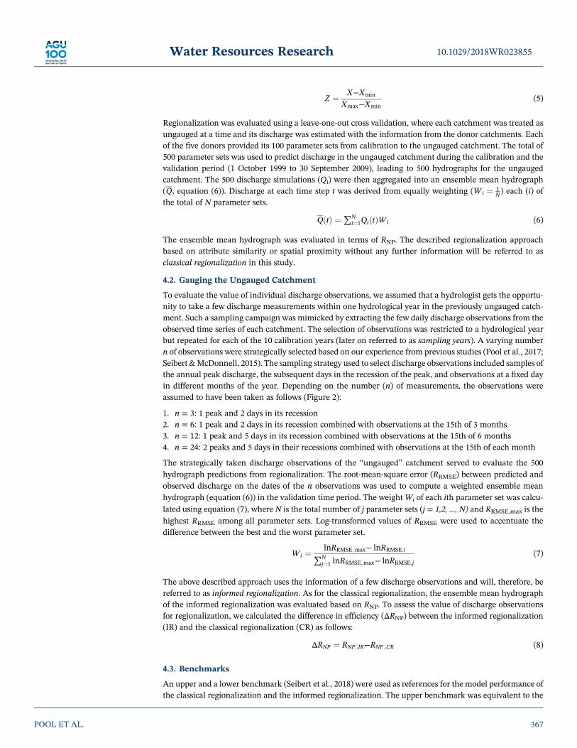
Mapping the effect of discharge observations on the classical regionalization allowed to visually separateregions where observations were highly informative from regions where they were less important(Figure 4). The map suggests that the value of observations varies in space. Discharge observations had noor only limited value in large parts of the central region of the eastern United States, such as the GulfCoast, the Mississippi Valley, and the Great Lakes Region. In contrast, a pronounced positive effect of dis-charge measurements was observed for the majority of catchments in the Appalachian Mountains and the

Figure 3. Model efficiency in validation for the 579 study catchments. (a) Model efficiency RNP for predictions with thelower (LB) and upper (UB) benchmark (yellow colors), and the classical and the informed regionalization (efficiencyof the median sampling year) with attribute similarity (green colors) and spatial proximity (blue colors). (b) Efficiencydifference (ΔRNP) between the classical and the informed regionalization, whereby positive values indicate an increase inprediction efficiency using information of a few discharge observations.

10.1029/2018WR023855Water Resources Research

POOL ET AL. 369

western United States. The described spatial pattern can also be observed when plotting the effect of dis-charge observations against catchment attributes (Figures 5a–5g and 6a–6g). Discharge observations didin general strongly improve classical regionalization in arid catchments that are most prominent in theSouthwest, and in snow‐dominated catchments in mountainous regions or northern latitudes.Furthermore, regionalization with spatial proximity was improved by the information of discharge observa-tions in catchments with a distinct winter precipitation season, which are catchments typically located alongthe West Coast.

In addition to the variable value of discharge observations as a function of catchment attributes, informationof a few observations was also more important when the distance between the ungauged catchment and itsdonors was relatively large (Figures 5h and 6h).

5.3. About the Information Content of Different Discharge Sampling Years

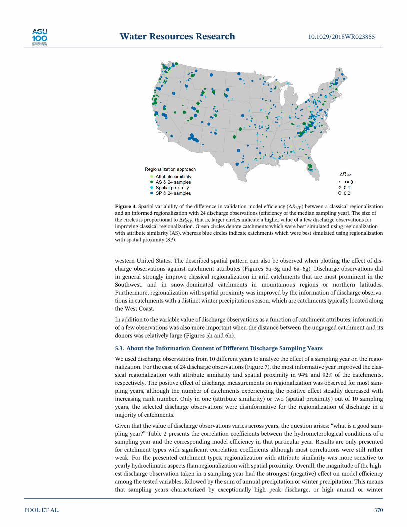
We used discharge observations from 10 different years to analyze the effect of a sampling year on the regio-nalization. For the case of 24 discharge observations (Figure 7), the most informative year improved the clas-sical regionalization with attribute similarity and spatial proximity in 94% and 92% of the catchments,respectively. The positive effect of discharge measurements on regionalization was observed for most sam-pling years, although the number of catchments experiencing the positive effect steadily decreased withincreasing rank number. Only in one (attribute similarity) or two (spatial proximity) out of 10 samplingyears, the selected discharge observations were disinformative for the regionalization of discharge in amajority of catchments.

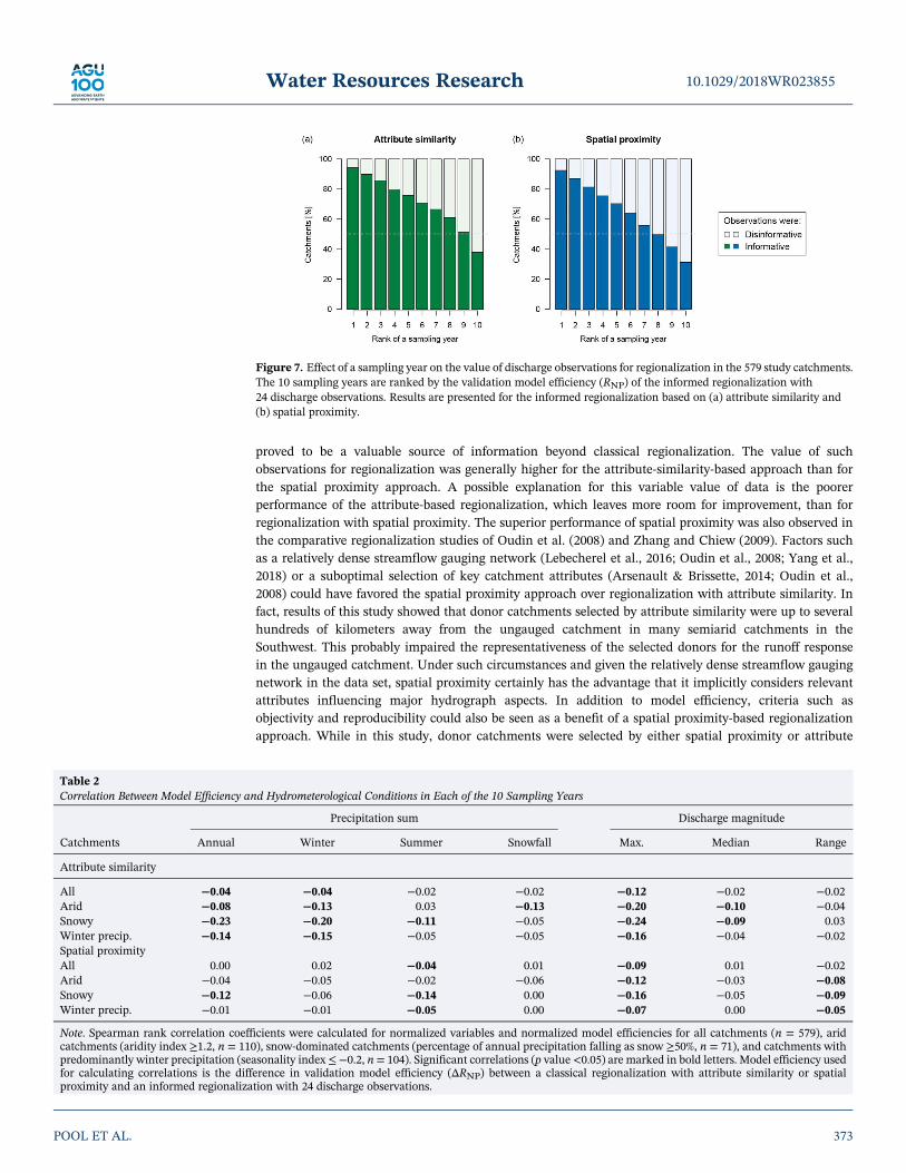
Given that the value of discharge observations varies across years, the question arises: “what is a good sam-pling year?” Table 2 presents the correlation coefficients between the hydrometerological conditions of asampling year and the corresponding model efficiency in that particular year. Results are only presentedfor catchment types with significant correlation coefficients although most correlations were still ratherweak. For the presented catchment types, regionalization with attribute similarity was more sensitive toyearly hydroclimatic aspects than regionalization with spatial proximity. Overall, the magnitude of the high-est discharge observation taken in a sampling year had the strongest (negative) effect on model efficiencyamong the tested variables, followed by the sum of annual precipitation or winter precipitation. This meansthat sampling years characterized by exceptionally high peak discharge, or high annual or winter

Figure 4. Spatial variability of the difference in validation model efficiency (ΔRNP) between a classical regionalizationand an informed regionalization with 24 discharge observations (efficiency of the median sampling year). The size ofthe circles is proportional to ΔRNP, that is, larger circles indicate a higher value of a few discharge observations forimproving classical regionalization. Green circles denote catchments which were best simulated using regionalizationwith attribute similarity (AS), whereas blue circles indicate catchments which were best simulated using regionalizationwith spatial proximity (SP).

10.1029/2018WR023855Water Resources Research

POOL ET AL. 370

precipitation were the least informative for regionalization of discharge in arid catchments, snow‐dominatedcatchments, and winter‐precipitation‐dominated catchments.

5.4. How Many Discharge Observations Are Needed?

Figure 8 presents the effect of the number of discharge observations on the regionalization. An increasingnumber of observations in the least informative year not only improved efficiencies but also clearly reducedthe variability in model performance between catchments. More importantly, with the use of more observa-tions, a sampling year could change from being mostly disinformative to being informative for a consider-able number of catchments. In a median year, median model performance only slightly increased with an

Figure 5. Difference in validation model efficiency (ΔRNP) between a regionalization with attribute similarity and an informed regionalization with 24 dischargeobservations (efficiency of the median sampling year) versus (a–g) catchment attributes and (h) the median distance in the attribute space between the“ungauged” catchment and its donors. Results are presented for all 579 study catchments, whereby positive efficiency difference indicates an increase in predictionefficiency using information of a few discharge observations. The lines represent averaged values of the median, the 25th quantile, and the 75th quantile over amoving window of 11 to 101 catchments (smaller moving windows were used at the lower and upper boundaries of the attribute data as indicated by thinner linestoward the boundaries).

10.1029/2018WR023855Water Resources Research

POOL ET AL. 371

increasing number of observations. However, informing regionalization with 24 instead of 3 observationsincreased the number of catchments that were better predicted by the informed regionalization by about10%. In the most informative year, 3 discharge observations had a comparable effect on modelperformance as 24 discharge observations.

6. Discussion

The result that a limited number of discharge observations can improve predictions in otherwise ungaugedcatchments is in agreement with Rojas‐Serna et al. (2016) and Viviroli and Seibert (2015), who concludedthat a few randomly selected discharge observations or a few observations during mean‐flow conditions

Figure 6. Difference in validation model efficiency (ΔRNP) between a regionalization with spatial proximity and an informed regionalization with 24 dischargeobservations (efficiency of the median sampling year) versus (a–g) catchment attributes and (h) the median distance between the “ungauged” catchment andits donors. Results are presented for all 579 study catchments, whereby positive efficiency difference indicates an increase in prediction efficiency using informationof a few discharge observations. The lines represent averaged values of the median, the 25th quantile and the 75th quantile over a moving window of 11 to 101catchments (smaller moving windows were used at the lower and upper boundaries of the attribute data as indicated by thinner lines toward the boundaries).

10.1029/2018WR023855Water Resources Research

POOL ET AL. 372

proved to be a valuable source of information beyond classical regionalization. The value of suchobservations for regionalization was generally higher for the attribute‐similarity‐based approach than forthe spatial proximity approach. A possible explanation for this variable value of data is the poorerperformance of the attribute‐based regionalization, which leaves more room for improvement, than forregionalization with spatial proximity. The superior performance of spatial proximity was also observed inthe comparative regionalization studies of Oudin et al. (2008) and Zhang and Chiew (2009). Factors suchas a relatively dense streamflow gauging network (Lebecherel et al., 2016; Oudin et al., 2008; Yang et al.,2018) or a suboptimal selection of key catchment attributes (Arsenault & Brissette, 2014; Oudin et al.,2008) could have favored the spatial proximity approach over regionalization with attribute similarity. Infact, results of this study showed that donor catchments selected by attribute similarity were up to severalhundreds of kilometers away from the ungauged catchment in many semiarid catchments in theSouthwest. This probably impaired the representativeness of the selected donors for the runoff responsein the ungauged catchment. Under such circumstances and given the relatively dense streamflow gaugingnetwork in the data set, spatial proximity certainly has the advantage that it implicitly considers relevantattributes influencing major hydrograph aspects. In addition to model efficiency, criteria such asobjectivity and reproducibility could also be seen as a benefit of a spatial proximity‐based regionalizationapproach. While in this study, donor catchments were selected by either spatial proximity or attribute

Figure 7. Effect of a sampling year on the value of discharge observations for regionalization in the 579 study catchments.The 10 sampling years are ranked by the validation model efficiency (RNP) of the informed regionalization with24 discharge observations. Results are presented for the informed regionalization based on (a) attribute similarity and(b) spatial proximity.

Table 2Correlation Between Model Efficiency and Hydrometerological Conditions in Each of the 10 Sampling Years

Catchments

Precipitation sum Discharge magnitude

Annual Winter Summer Snowfall Max. Median Range

Attribute similarity

All −0.04 −0.04 −0.02 −0.02 −0.12 −0.02 −0.02Arid −0.08 −0.13 0.03 −0.13 −0.20 −0.10 −0.04Snowy −0.23 −0.20 −0.11 −0.05 −0.24 −0.09 0.03Winter precip. −0.14 −0.15 −0.05 −0.05 −0.16 −0.04 −0.02Spatial proximityAll 0.00 0.02 −0.04 0.01 −0.09 0.01 −0.02Arid −0.04 −0.05 −0.02 −0.06 −0.12 −0.03 −0.08Snowy −0.12 −0.06 −0.14 0.00 −0.16 −0.05 −0.09Winter precip. −0.01 −0.01 −0.05 0.00 −0.07 0.00 −0.05

Note. Spearman rank correlation coefficients were calculated for normalized variables and normalized model efficiencies for all catchments (n = 579), aridcatchments (aridity index ≥1.2, n = 110), snow‐dominated catchments (percentage of annual precipitation falling as snow ≥50%, n = 71), and catchments withpredominantly winter precipitation (seasonality index ≤−0.2, n= 104). Significant correlations (p value <0.05) are marked in bold letters. Model efficiency usedfor calculating correlations is the difference in validation model efficiency (ΔRNP) between a classical regionalization with attribute similarity or spatialproximity and an informed regionalization with 24 discharge observations.

10.1029/2018WR023855Water Resources Research

POOL ET AL. 373

similarity, attempts of combining both approaches have been shown to be a promising approach for theselection of potential donor catchments (Buytaert & Beven, 2009; Oudin et al., 2008; Samuel et al., 2011;Yang et al., 2018; Zhang & Chiew, 2009).

Independent of the classical regionalization approach, discharge observations were most informative in aridcatchments, snow‐dominated catchments, and winter‐precipitation‐dominated catchments. These catch-ments generally have a distinct runoff regime with a pronounced high‐flow period. The discharge observa-tions selected to inform the regionalization in this study were sampled during these periods of high flow.They therefore provided information for the regionalization at a time when dominant runoff processes wereactive. These results are comparable to those of Viviroli and Seibert (2015), who reported that dischargeobservations during the snowmelt and ice melt season were most valuable for informing regionalizationin snow‐dominated or glaciated catchments. They furthermore showed that more observations were neededto effectively inform regionalization for catchments with a predominantly pluvial regime because of therandomness of rain events between and within years as opposed to the reoccurring process of snowmeltand ice melt. The variability in precipitation and the related timing of the dominant runoff processes couldalso provide an explanation for the limited value of discharge observations found in large parts of the centralregion of the eastern United States.

The value of discharge observations for the regionalization varied across sampling years, whereby years withhigh sums of annual or winter precipitation and therefore relatively high discharge events were the leastinformative ones. This was unexpected at first, because it has been shown that runoff models could becalibrated with a limited number of discharge observations, especially if they were sampled during wetperiods (Melsen et al., 2014; Vrugt et al., 2006; Yapo et al., 1996) or peak events (Pool et al., 2017; Seibert&McDonnell, 2015) when dominant runoff processes were active. However, under unusually wet conditionsspecial runoff processes might govern catchment runoff responses. Using discharge observations takenduring such unusual conditions can inform the regionalization with data of limited representativeness,which ultimately favors parameter sets that reproduce rather exceptional runoff responses. However, it isimportant to note that the correlations between the value of observations and the hydrometeorological con-ditions in a sampling year were rather weak and only significant for arid catchments, snow‐dominatedcatchments, and winter‐precipitation‐dominated catchments. These results therefore have to be interpretedwith some caution. More detailed insights into the value of individual sampling years could be gained by aninductive approach that addresses the influence of large‐scale climate phenomena such as El Niño–SouthernOscillation, rating curve uncertainties affecting the value of discharge observations at peak flows, ordisinformation at the event level introduced by a mismatch between precipitation input and runoff response(Beven & Westerberg, 2011). However, such an in‐depth analysis on the value of sampling years was notconducted within this study.

Figure 8. Effect of the number of discharge observation on the difference in validationmodel efficiency (ΔRNP) between aclassical regionalization and an informed regionalization in the 579 study catchments. The effect of a variable numberof observations on regionalization with (a) attribute similarity and (b) spatial proximity is presented for the mostinformative sampling year, the median sampling year, and the least informative sampling year. Positive efficiencydifferences (ΔRNP) indicate an increase in prediction efficiency using information of a few discharge observations.

10.1029/2018WR023855Water Resources Research

POOL ET AL. 374

The sampling year not only influenced model performance but also affected the number of observationsneeded to inform regionalization. Increasing the number of discharge observations strongly improved regio-nalization for observations collected in the least informative year, probably because the effect of an indivi-dual unusual event could be balanced by additional and more representative observations. In contrast, thecharacteristic runoff response could be captured by as few as three observations if these observations werecollected in the most informative sampling year.

The results of this study are based on the strategic extraction of a few discharge observations from theobserved time series of catchments and therefore provide insights in what could be achieved at best. In prac-tice, decisions on the number of observations, the dates of observations, or the sampling year may berestricted by economical or organizational factors. Cost‐benefit analysis for real case studies could be away to bridge the gap between the theoretical and practical value of a limited number of discharge observa-tions for the prediction in ungauged catchments.

An additional practical limitation of this study is the fact that discharge observations used to inform regio-nalization correspond to mean daily values, whereas observations collected during field campaigns arealmost instantaneous. The differences between instantaneous discharge values (reported discharge data at15‐min interval) and mean daily discharge were looked at for eight catchments representing the typicalrange of catchment areas (10, 100, 1,000, and 10,000 km2) encountered in the CAMELS data set. Therebyit could be observed that mean daily discharge can deviate considerably from instantaneous discharge obser-vations at days with peak flows. However, instantaneous measurements can be regarded as representativefor the mean daily values during most other periods including event recessions and low flow periods whenwithin‐day flow variations are relatively small. Similarly, a more detailed analysis of the value of subdailydischarge observations by Viviroli and Seibert (2015) indicated a limited added value of several subsequentinstantaneous discharge observations within a few hours.

7. Conclusions

Many catchments lack continuous discharge time series and the prediction of discharge relies on regionali-zation. However, it might still be possible to collect a limited number of discharge observations during shortfield campaigns. In this study, we evaluated the value of such a limited number of discharge observations forinforming parameter regionalization using a large‐sample data set of the United States. Results demon-strated that a few discharge observations improved regionalization in the majority of catchments and thatobservations were especially effective in arid catchments, snow‐dominated catchments, and winter‐precipi-tation‐dominated catchments. Discharge observations from years with moderate to low peak flow magni-tudes were the most informative ones, whereby 3 observations could be of comparable value as 24observations if collected in these most informative years. The results demonstrate the value of a small num-ber of streamflow observations and indicate that short field campaigns can improve the basis for decisionmaking in ungauged basins.

ReferencesAddor, N., Newman, A. J., Mizukami, N., & Clark, M. P. (2017). The CAMELS data set: Catchment attributes and meteorology for large‐

sample studies. Hydrology and Earth System Sciences, 21(10), 5293–5313. https://doi.org/10.5194/hess‐21‐5293‐2017Arsenault, R., & Brissette, F. (2014). Continuous streamflow prediction in ungauged basins: The effects of equifinality and parameter set

selection on uncertainty in regionalization approaches. Water Resources Research, 50, 6135–6153. https://doi.org/10.1002/2013WR014898

Bárdossy, A. (2007). Calibration of hydrological model parameters for ungauged catchments. Hydrology and Earth System Sciences, 11(2),703–710. https://doi.org/10.5194/hess‐11‐703‐2007

Bergström, S. (1976). Development and application of a conceptual runoff model for Scandinavian catchments. Norrköping, Sweden: SMHI.Beven, K., & Freer, J. (2001). Equifinality, data assimilation, and uncertainty estimation in mechanistic modelling of complex envir-

onmental systems using the GLUE methodology. Journal of Hydrology, 249(1–4), 11–29. https://doi.org/10.1016/S0022‐1694(01)00421‐8

Beven, K., & Westerberg, I. (2011). On red herrings and real herrings: Disinformation and information in hydrological inference.Hydrological Processes, 25(10), 1676–1680. https://doi.org/10.1002/hyp.7963

Blöschl, G., & Sivapalan, M. (1995). Scale issues in hydrological modelling: A review.Hydrological Processes, 19(11), 4559–4579. https://doi.org/10.5194/hess‐19‐4559‐2015.

Burn, D. H. (1990). Evaluation of regional flood frequency analysis with a region of influence approach.Water Resources Research, 26(10),2257–2266. https://doi.org/10.1029/90WR01192

Burn, D. H., & Boorman, D. B. (1993). Estimation of hydrological parameters at ungauged catchments. Journal of Hydrology, 143(3–4),429–454. https://doi.org/10.1016/0022‐1694(93)90203‐L

10.1029/2018WR023855Water Resources Research

POOL ET AL. 375

AcknowledgmentsThis work was supported by theUniversity of Zurich.Hydrometeorological data, catchmentattributes, and catchment boundarieswere made available by Addor et al.(2017) and Newman et al. (2015). SRTMelevation data were used from Jarviset al. (2008), and data on thedistribution of wetlands were extractedfrom the data set of Lehner and Döll(2004).

Buytaert, W., & Beven, K. (2009). Regionalization as a learning process. Water Resources Research, 45, W11419. https://doi.org/10.1029/2008WR007359

Gupta, H. V., Kling, H., Yilmaz, K. K., & Martinez, G. F. (2009). Decomposition of the mean squared error and NSE performancecriteria: Implications for improving hydrological modelling. Journal of Hydrology, 377(1–2), 80–91. https://doi.org/10.1016/j.jhydrol.2009.08.003

Harlin, J. (1991). Development of a process oriented calibration scheme for the HBV hydrological model. Nordic Hydrology, 22(1), 15–36.https://doi.org/10.2166/nh.1991.002.

He, Y., Bárdossy, A., & Zehe, E. (2011). A review of regionalisation for continuous streamflow simulation. Hydrology and Earth SystemSciences, 15(11), 3539–3553. https://doi.org/10.5194/hess‐15‐3539‐2011

Hrachowitz, M., Savenije, H. H. G., Blöschl, G., McDonnell, J. J., Sivapalan, M., Pomeroy, J. W., Arheimer, B., et al. (2013). A decade ofpredictions in ungauged basins (PUB)—A review. Hydrological Sciences Journal, 58(6), 1198–1255. https://doi.org/10.1080/02626667.2013.803183

Jarvis, A., Reuter, H., Nelson, A., & Guevara, E. (2008). Hole‐filled SRTM for the globe Version 4, available from the CGIAR‐CSI SRTM90m. Retrieved from http://srtm.csi.cgiar.org

Kokkonen, T. S., Jakeman, A. J., Young, P. C., & Koivusalo, H. J. (2003). Predicting daily flows in ungauged catchments: Model regiona-lization from catchment descriptors at the Coweeta Hydrologic Laboratory, North Carolina. Hydrological Processes, 17(11), 2219–2238.https://doi.org/10.1002/hyp.1329

Lebecherel, L., Andréassian, V., & Perrin, C. (2016). On evaluating the robustness of spatial‐proximity‐based regionalization methods.Journal of Hydrology, 539, 196–203. https://doi.org/10.1016/j.jhydrol.2016.05.031

Lehner, B., & Döll, P. (2004). Development and validation of a global database of lakes, reservoirs and wetlands. Journal of Hydrology,296(1–4), 1–22. https://doi.org/10.1016/j.jhydrol.2004.03.028

Lindström, G., Johansson, B., Persson, M., Gardelin, M., & Bergström, S. (1997). Development and test of the distributed HBV‐96 hydro-logical model. Journal of Hydrology, 201(1–4), 272–288. https://doi.org/10.1016/S0022‐1694(97)00041‐3

McIntyre, N., Lee, H., Wheater, H., Young, A., & Wagener, T. (2005). Ensemble predictions of runoff in ungauged catchments. WaterResources Research, 41, W12434. https://doi.org/10.1029/2005WR004289

Melsen, L. A., Teuling, A. J., van Berkum, S.W. S., Torfs, P. J. J. F., &Uijlenhoet, R. (2014). Catchments as simple dynamical systems: A casestudy onmethods and data requirements for parameter identification.Water Resources Research, 50, 5577–5596. https://doi.org/10.1002/2013WR014720

Merz, R., & Blöschl, G. (2004). Regionalisation of catchment model parameters. Journal of Hydrology, 287(1–4), 95–123. https://doi.org/10.1016/j.jhydrol.2003.09.028

Milligan, G. W., & Cooper, M. C. (1988). A study of standardization of variables in cluster analysis. Journal of Classification, 5(2), 181–204.https://doi.org/10.1007/BF01897163.

Nash, J. E., & Sutcliffe, J. V. (1970). River flow forecasting through conceptual models. Part I—A discussion of principles. Journal ofHydrology, 10(3), 282–290. https://doi.org/10.1016/0022‐1694(70)90255‐6

Newman, A. J., Clark, M. P., Sampson, K., Wood, A., Hay, L. E., Bock, A., Viger, R. J., et al. (2015). Development of a large‐samplewatershed‐scale hydrometeorological data set for the contiguous USA: Data set characteristics and assessment of regional variability inhydrologic model performance. Hydrology and Earth System Sciences, 19(1), 209–223. https://doi.org/10.5194/hess‐19‐209‐2015

Oudin, L., Andréassian, V., Perrin, C., Michel, C., & Le Moine, N. (2008). Spatial proximity, physical similarity, regression and ungagedcatchments: A comparison of regionalization approaches based on 913 French catchments. Water Resources Research, 44, W034135.https://doi.org/10.1029/2007WR006240

Parajka, J., Viglione, A., Rogger, M., Salinas, J. L., Sivapalan, M., & Blöschl, G. (2013). Comparative assessment of predictions in ungaugedbasins—Part 1: Runoff‐hydrograph studies. Hydrology and Earth System Sciences, 17(5), 1783–1795. https://doi.org/10.5194/hess‐17‐1783‐2013

Pool, S., Vis, M., & Seibert, J. (2018). Evaluating model performance: Towards a non‐parametric variant of the Kling‐Gupta efficiency.Hydrological Sciences Journal https://doi.org/10.1080/02626667.2018.1552002, 63(13‐14), 1941–1953.

Pool, S., Viviroli, D., & Seibert, J. (2017). Prediction of hydrographs and flow‐duration curves in almost ungauged catchments: Whichrunoff measurements are most informative for model calibration? Journal of Hydrology, 554, 613–622. https://doi.org/10.1016/j.jhydrol.2017.09.037

Priestley, C. H. B., & Taylor, R. J. (1972). On the assessment of surface heat flux and evaporation using large‐scale parameters. MonthlyWeather Review, 100(2), 81–92. https://doi.org/10.1175/1520‐0493(1972)100<0081:OTAOSH>2.3.CO;2

Razavi, T., & Coulibaly, P. (2013). Streamflow prediction in ungauged basins: Review of regionalization methods. Journal of HydrologicEngineering, 18(8), 958–975. https://doi.org/10.1061/(ASCE)HE.1943‐5584.0000690

Rojas‐Serna, C., Lebecherel, L., Perrin, C., Andréassian, V., & Oudin, L. (2016). How should a rainfall‐runoff model be parameterized in analmost ungauged catchment? A methodology tested on 609 catchments. Water Resources Research, 52, 4765–4784. https://doi.org/10.1002/2015WR018549

Samuel, J., Coulibaly, P., & Metcalfe, R. A. (2011). Estimation of continuous streamflow in Ontario ungauged basins: Comparison ofregionalization methods. Journal of Hydrologic Engineering, 16(5), 447–459. https://doi.org/10.1061/(ASCE)HE.1943‐5584.0000338

Seibert, J. (2000). Multi‐criteria calibration of a conceptual runoff model using a genetic algorithm. Hydrology and Earth System Sciences,4(2), 215–224. https://doi.org/10.5194/hess‐4‐215‐2000

Seibert, J., & Beven, K. J. (2009). Gauging the ungauged basin: How many discharge measurements are needed? Hydrology and EarthSystem Sciences, 13(6), 883–892. https://doi.org/10.5194/hess‐13‐883‐2009

Seibert, J., & McDonnell, J. J. (2015). Gauging the ungauged basin: Relative value of soft and hard data. Journal of Hydrologic Engineering,20(1), A4014004. https://doi.org/10.1061/(ASCE)HE.1943‐5584.0000861

Seibert, J., & Vis, M. J. P. (2012). Teaching hydrological modeling with a user‐friendly catchment‐runoff‐model software package.Hydrology and Earth System Sciences, 16(9), 3315–3325. https://doi.org/10.5194/hess‐16‐3315‐2012

Seibert, J., Vis, M. J. P., Lewis, E., & van Meerveld, H. J. (2018). Upper and lower benchmarks in hydrological modelling. HydrologicalProcesses, 32(8), 1120–1125. https://doi.org/10.1002/hyp.11476

Singh, S. K., & Bárdossy, A. (2012). Calibration of hydrological models on hydrologically unusual events. Advances in Water Resources, 38,81–91. https://doi.org/10.1016/j.advwatres.2011.12.006

Sivapalan, M., Takeuchi, K., Franks, S. W., Gupta, V. K., Karambiri, H., Lakshmi, V., Liang, X., et al. (2003). IAHS decade on Predictions inUngauged Basins (PUB), 2003–2012: Shaping an exciting future for the hydrological sciences. Hydrological Sciences Journal, 48(6),857–880. https://doi.org/10.1623/hysj.48.6.857.51421

10.1029/2018WR023855Water Resources Research

POOL ET AL. 376

Tobler, W. R. (1970). A computermovie simulating urban growth in the Detroit Region. Economic Geography, 11(277), 620–622. https://doi.org/10.1126/science.11.277.620

Viviroli, D., Mittelbach, H., Gurtz, J., & Weingartner, R. (2009). Continuous simulation for flood estimation in ungauged mesoscalecatchments of Switzerland—Part II: Parameter regionalisation and flood estimation results. Journal of Hydrology, 377(1‐2), 208–225.https://doi.org/10.1016/j.jhydrol.2009.08.022

Viviroli, D., & Seibert, J. (2015). Can a regionalized model parameterisation be improved with a limited number of runoff measurements?Journal of Hydrology, 529, 49–61. https://doi.org/10.1016/j.jhydrol.2015.07.009

Vrugt, J. A., Gupta, H. V., Dekker, S. C., Sorooshian, S., Wagener, T., & Bouten,W. (2006). Application of stochastic parameter optimizationto the Sacramento Soil Moisture Accounting model. Journal of Hydrology, 325(1–4), 288–307. https://doi.org/10.1016/j.jhydrol.2005.10.041

Yang, X., Magnusson, J., Rizzi, J., & Xu, C.‐Y. (2018). Runoff prediction in ungauged catchments in Norway: Comparison of regionalizationapproaches. Hydrology Research, 49(2), 487–505. https://doi.org/10.2166/nh.2017.071

Yapo, P. O., Gupta, H. V., & Sorooshian, S. (1996). Automatic calibration of conceptual rainfall‐runoff models: Sensitivity to calibrationdata. Journal of Hydrology, 181(1–4), 23–48. https://doi.org/10.1016/0022‐1694(95)02918‐4

Zhang, Y., & Chiew, F. H. S. (2009). Relative merits of different methods for runoff predictions in ungauged catchments. Water ResourcesResearch, 45, W07412. https://doi.org/10.1029/2008WR007504

10.1029/2018WR023855Water Resources Research

POOL ET AL. 377