Value versus Growth Investing:

Why Do Different Investors Have Different Styles?∗

Henrik Cronqvist, Stephan Siegel, and Frank Yu†

This draft: November 7, 2013

Abstract

We find that several factors explain an investor’s style, i.e., the value versus growth orienta-tion of the investor’s stock portfolio. First, an investor’s style has a biological basis – a pref-erence for value versus growth stocks is partially ingrained in an investor already from birth.Second, investors who a priori are expected to take more financial risk (e.g., men and wealth-ier individuals) have a preference for growth, not value, which may be surprising if the valuepremium reflects risk. Finally, an investor’s style is explained by life course theory in that ex-periences, both earlier and later in life, are related to investment style. Investors with adversemacroeconomic experiences (e.g., growing up during the Great Depression or entering the jobmarket during an economic downturn) and those who grew up in a lower status socio-economicrearing environment have a stronger value orientation several decades later in their lives. Ourresearch contributes a new perspective to the long-standing value/growth debate in finance.

∗We are thankful for comments from seminar participants at China Europe International Business School, ShanghaiAdvanced Institute of Finance, and for discussions with Colin Camerer, Augustin Landier, Feng Li, Stefan Nagel,Jun Qian, Meir Statman, and Tan Wang. We thank S&P Capital IQ’s China and Hong Kong teams (in particularRick Chang) for help with various data issues. We also thank Wenqian Hu, Lucas Perin, and Nancy Yao for capableresearch assistance. This project has been supported by generous research funding from China Europe InternationalBusiness School (CEIBS). Statistics Sweden and the Swedish Twin Registry (STR) provided the data for this study.STR is supported by grants from the Swedish Research Council, the Ministry of Higher Education, AstraZeneca, andthe National Institute of Health (grants AG08724, DK066134, and CA085739). This project was pursued in part whenCronqvist was Olof Stenhammar Visiting Professor at the Swedish Institute for Financial research (SIFR), which hethanks for its support. Any errors or omissions are our own.†Cronqvist and Yu: China Europe International Business School (hcronqvist@ceibs.edu and fyu@ceibs.edu); Siegel:

University of Washington, Michael G. Foster School of Business (ss1110@uw.edu).

I think Warren [Buffett] captured the idea himself in his 1964 article “The Superinvestors of Grahamand Doddsville” and in it he talks about – value investing is like an inoculation – you either get itright away, or you never get it. And I think it’s just true. I actually think there’s just a gene forthis stuff, whether it’s a value investing gene or a contrarian gene.

— Seth Klarman, in an interview with Charlie Rose, 2011.

I Introduction

The concepts of “value” and “growth” investing have a long history in financial economics. Today,

there exist some 2,050 value funds and 3,200 growth funds catering to investors with preferences for

these investment styles.1 Fidelity, the world’s largest provider of employer-sponsored retirement plans

such as 401(k) plans, prominently features a description of value and growth funds on their Learning

Center website.2 For more than two decades, Morningstar has provided a Value-Growth Score to

help investors choose a fund with their preferred style. There are best-selling books about both

value and growth strategies, and countless business magazine articles boast recommendations about

the “Best Value Funds” and/or the “Best Growth Funds.” Wall Street professionals are educated

about value and growth investing already in business school, with many MBA programs today

offering (very popular) courses on, e.g., Value Investing. Most importantly from the perspective

of academic research, one of the most debated issues in the past several decades is the differential

returns of investments in value versus growth stock portfolios – the value premium debate (e.g.,

De Bondt and Thaler (1985), Fama and French (1992, 1993, 1996), Lakonishok, Shleifer, and Vishny

(1994), and Daniel and Titman (1997)).3

Despite all this attention to value and growth investing, very little research has attempted to

explain the determinants of an individual’s investment style. That is, why are some investors value

oriented, while others are growth oriented? In this paper, we argue that differences in investment

styles across individuals, in principle, may stem from either of two non-mutually exclusive sources.

First, these differences may be biological, in the sense that a gene, or most likely a combination

1Morningstar.com.2https://www.fidelity.com/learning-center/mutual-funds/growth-vs-value-investing.3This debate has not been limited to only the U.S. stock market, but extended to several other markets as well

(e.g., Chan et al. (1991), Fama and French (1998), and Daniel et al. (2001)).

1

of several genes, result in a preference for a specific investment style. In recent years, individual

characteristics of first-order importance for portfolio choice, e.g., the propensity to take financial

risk, have indeed been shown to be partly explained by an individual’s genetic composition (e.g.,

Cesarini et al. (2009), Barnea, Cronqvist, and Siegel (2010) and Cesarini et al. (2010)). As a result,

we hypothesize that an individual’s investment style has a biological basis, i.e., a preference for

value versus growth stocks is partially ingrained in an investor from birth.

Second, based on life course theory, an approach to research in social psychology,4 which has

recently made its way into economics and finance research (e.g., Oyer (2006, 2008), Kaustia and

Knupfer (2008), Malmendier and Nagel (2011, 2013), and Schoar and Zuo (2013)), we hypothesize

that an individual’s specific life experiences affect behaviors, including the individual’s investment

style, later in life. We consider several potentially relevant, and exogenous, life experiences of

individuals: 1) Macroeconomic experiences, 2) Impressionable years, and 3) Rearing environment.

More specifically, we examine whether experiencing an adverse and significant macroeconomic event,

e.g., growing up during the Great Depression, affects an individual’s value versus growth orientation.

We also analyze other impressionable years during an individual’s life course, e.g., the economic

conditions when an individual entered the job market for the first time. Finally, we also examine

the socio-economic status of the rearing environment in which the individual grew up.

Benjamin Graham and T. Rowe Price, Jr., constitute a colorful illustration of some of our

hypotheses. Graham is commonly dubbed the “Father of Value Investing” because he preferred

stocks with comparatively low valuation ratios and other characteristics that subsequently came to

define value investing. Price, the founder of the large money management company with his name,

is often referred to as the “Father of Growth Investing” because of his preference for companies

characterized by strong earnings growth, R&D intensity, and innovative technology. So why did

Graham become a value investor, while Price became a growth investor? Their different investment

styles may very well have a biological basis, but this is not possible to examine without data on their

genetic differences. Interestingly, Graham grew up very poor, his father passing away unexpectedly

when he was young, and his mother losing the family’s savings in the Panic of 1907. Among his

4For further details and references, see, e.g., Giele and Elder (1998) and Elder et al. (2003).

2

brothers, Graham was often tasked with “bargain hunting” at different grocery stores (e.g., Carlen

(2012)). In comparison, Price had a privileged upbringing, his father being an M.D. who served as a

surgeon his entire professional career for a rapidly expanding railroad company, a growth company

at that time. We hypothesize that their different life experiences contributed to their different

investment styles.

To empirically decompose variation in investment styles across a large sample of individual

investors we use two ingredients. First, we employ data on identical and fraternal twins from the

world’s largest twin registry, the Swedish Twin Registry (STR), matched with detailed data on

these individuals’ stock and mutual fund portfolios from the Swedish Tax Agency. Data on twins

are commonly used for decomposition of variation across individuals into genetic and environmental

sources.5 We do not expect a dichotomous classification of value versus growth investors to be

empirically relevant so we categorize each investor’s value versus growth “orientation” on a continuum.

Second, we use empirical methods from quantitative behavioral genetics research which have recently

been employed also in research in economics (e.g., Cesarini et al. (2009)). This methodology involves

maximum likelihood estimation of a random effects model, but relies on an intuitive and simple

insight: Identical twins share 100% of their genes, while the average proportion of shared genes is

only 50% for fraternal twins, so if identical twins are more similar with respect to their investment

styles than are fraternal twins, then there is evidence that value versus growth orientation is partly

explained by genetic predispositions. To preview our findings, the correlation among identical twins

is 0.32 for the average price-to-earnings (P/E) ratio of the stock portfolio, compared to only 0.20

among same-sex fraternal twins; the corresponding correlations are 0.30 versus 0.16 for the average

Value-Growth Score by Morningstar for the mutual fund portfolio. That is, genetically more similar

investors have more similar investment styles.

Our research contributes a new perspective to the long-standing value/growth debate in finance.

First, an investor’s style has a biological basis – a preference for value versus growth stocks is

partially ingrained in an investor already from birth. We estimate that genetic differences across

individuals explain 18% of the cross-sectional variation in value versus growth orientation, if using

5Research in economics has a long tradition of using data on twins; see, e.g., Behrman and Taubman (1976, 1989),Taubman (1976), Ashenfelter and Krueger (1994), and Black et al. (2007).

3

P/E ratios as an investment style measure, and 25% if using Morningstar’s Value-Growth Score.

Second, investors who a priori are expected to take more financial risk have a preference for growth,

not value, investing. This result is consistently found in data for exogenous proxies for risk taking

propensity (e.g., gender and age) and also other individual characteristics (e.g., wealth). If value is

riskier than growth, it may be surprising that those who are expected to take more (less) financial

risk prefer growth (value) stock portfolios. Finally, an investor’s style is explained by life course

theory in that experiences, both earlier and later in life, are related to investment style. In particular,

investors with adverse macroeconomic experiences have stronger preferences for value investing later

in life. For example, those who grew up during the Great Depression have portfolios with average

P/E ratios that are 2.2 (or about 10% at the median) lower, controlling for individual characteristics,

several decades later in life. Consistent with an impressionable years hypothesis, those who enter

the job market for the first time during an economic downturn are also more value oriented later on.

We also find that those who grew up in a lower status socio-economic rearing environment also have

a stronger value orientation later in life.

The paper is organized as follows. Section II reviews related research. Section III introduces our

data, and Section IV our empirical methodology. Section V reports our results. Section VI discusses

potential implications of our results, and Section VII concludes.

II Related Research

A Biological Predispositions and Investment Style

A.1 Risk Preferences

In standard models in financial economics, value and growth reflect differences in risk. A well-

established empirical result is that a value/growth risk factor, referred to as HML (“high minus low”)

following the seminal work by Fama and French (1993), is a significant determinant of cross-sectional

returns of stock portfolios. Different stocks and portfolios have different exposures to this HML

factor, and as a result, different expected returns. If value-oriented portfolios have outperformed

growth-oriented portfolios historically because of differences in risk, we would expect investors with

4

a propensity to take more (less) financial risk to prefer value (growth) stocks and mutual funds.

Several recent studies have shown that a significant portion, or about 30%, of the cross-sectional

variation in financial risk preferences is explained by biological predispositions. It is important to

emphasize that risk-taking in those studies is not defined from the perspective of exposure to a

value/growth risk factor, but risk preferences are either elicited from experiments (e.g., Cesarini

et al. (2009)) or involve measures such as the share in equities (e.g., Barnea, Cronqvist, and Siegel

(2010) and Cesarini et al. (2010)).6 Some research in the intersection of finance and neuroscience

has even identified specific candidate genes involved in explaining differences in financial risk taking

across individuals (e.g., Kuhnen and Chiao (2009), Dreber et al. (2009), and Zhong et al. (2009)).7

The aforementioned studies suggest a relation between, on the one hand, biological predispositions,

and on the other hand, risk preferences. As a result, if we find that genetic differences across

investors explain their value versus growth orientation, differential genetic propensities to financial

risk taking is a potential explanation which would be consistent with standard models in finance.

A.2 Behavioral Biases

While there is consensus among most financial economists that value stocks historically have

produced higher returns than growth stocks, the interpretation of why this is the case is much

more controversial.8 For example, Lakonishok, Shleifer, and Vishny (1994) argue that the return of

growth, or “glamour,” stocks is the result of investor sentiment, and provide evidence that value

stocks produce higher returns because they exploit some of the “behavioral biases” of investors, and

not because of risk. Daniel and Titman (1997) show that the return premium on value stocks does

not arise because of the comovement of these stocks with a risk factor – it is the characteristics,

rather than the covariance structure of returns, that explain the cross-sectional variation in stock

returns. In behavioral models, the value premium reflects positive feedback trading (e.g., De Long,

Shleifer, Summers, and Waldmann (1990), Hong and Stein (1999), and Barberis and Shleifer (2003)),

6Standard models show that, in a frictionless market, differences in risk preferences explain cross-sectional variationin the share in equities (e.g., Merton (1969) and Samuelson (1969)).

7The even deeper question is why risk preferences are genetic. Some of the theoretical work by Robson (2001b)addresses fundamental questions such as why nature has endowed individuals with utility functions. For further detailsand references, we refer to Robson (2001a).

8For a review of empirical evidence related to value and growth investing, see, e.g., Chan and Lakonishok (2004).

5

conservatism and representativeness (e.g., Barberis, Shleifer, and Vishny (1998)), or overconfidence

(e.g., Daniel, Hirshleifer, and Subrahmanyam (1998) and Daniel, Titman, and Wei (2001)).

Recent research suggests a relation between, on the one hand, biological predispositions, and on

the other hand, the aforementioned behavioral biases (e.g., Cesarini et al. (2012) and Cronqvist and

Siegel (2013)). As a result, if we find that genetic differences across investors explain their value

versus growth orientation, differential genetic behavioral biases is a potential explanation which

would be consistent with behavioral finance models.9

B Life Course Theory and Investment Style

B.1 Macroeconomic Experiences

Experiencing an adverse and significant macroeconomic event may have pervasive effects on an

individual’s behaviors later in life.10 In their “Depression Babies” study, Malmendier and Nagel

(2011) show that individuals who have experienced relatively low stock market returns in their

lives subsequently do not participate in the stock market and they take significantly less financial

risk if they do participate. Other economists have also found that macro events have long-term

effects on individual preferences. For example, Alesina and Fuchs-Schuendeln (2005) examine the

experiment of German reunification and find that East Germans (particularly older cohorts) have

stronger preferences for, e.g., redistribution than West Germans post-reunification. Malmendier and

Nagel (2013) show that differences in life experiences of high or low inflation predict differences in

subjective inflation expectations and also preferences for fixed versus variable rate investments.

If an adverse macroeconomic experience results in less risk taking later in life, and if value is

riskier than growth investing, we would expect investors who grew up during the Great Depression

to prefer growth investing. An alternative hypothesis, not necessarily based on a risk explanation, is

9Some of the theoretical work by Rayo and Becker (2007) and Brennan and Lo (2011) addresses why behaviors,even if not rational as defined in standard economic models, may survive human evolution. For further details andreferences, see, e.g., Cosmides and Tooby (1994), Chen et al. (2006), and Santos and Chen (2009).

10The Great Depression is the macro event that has so far been studied most in-depth in the social sciences,and a variety of outcomes later in life have been examined. We refer to Elder (1974) for one of the first and mostcomprehensive studies of the long-term effects of the Great Depression. Many researchers have argued that theGreat Depression created a “depression generation,” whose behavior affected the macroeconomy for decades afterthe depression ended. For example, Friedman and Schwartz (1963) suggested that the Great Depression “shattered”beliefs in capitalism.

6

that those who have more salient experiences of difficult economic conditions develop a value-oriented

investment style, with a preference for relatively “cheaper” stocks.

B.2 Impressionable Years

A growing number of studies in social psychology suggest that experiences in early adulthood are

particularly important for preferences later in life (e.g., Krosnick and Alwin (1989)). An individual’s

core attitudes, beliefs, and preferences crystallize during a period of great neurological plasticity in

early adulthood – the so-called “impressionable years” – and remain largely unchanged afterwards.

Recently, this research has made its way into economics and finance. For example, Giuliano and

Spilimbergo (2013) show that experiencing an economic downturn during the impressionable years

affects redistribution and political preferences later in life.

In this study, we focus on whether an individual started his or her first employment in an

economic downturn. This measure comes with the caveat that it is less exogenous compared to a

birth cohort measure such as the Great Depression because individuals may to some extent choose

when they enter the job market by increasing their investment in education edogenously. We still

find it informative to examine the time of an individual’s first employment because it has been

shown to be important in several studies for other economic outcomes (e.g., Oyer (2006, 2008),

Malmendier et al. (2011), Oreopoulos et al. (2012), and Schoar and Zuo (2013)). This is also a

period in their lives when many individuals start to invest in stocks and mutual funds.

B.3 Rearing Environment

The hypothesis that the rearing environment, and other early-life experiences, may have significant

long-term effects on an individual’s behaviors later in life has recently made its way into economic

research. Most existing studies examine outcomes such as education and earnings. For example,

economists have shown that birth order and family size (e.g., Black et al. (2005)) and birth weight

(e.g., Black et al. (2007)) affect educational attainment and earnings later in life.11 Relatively few

studies examine outcomes of primary interest to financial economists. One exception is Chetty et al.

11For a review of the causes and consequences of inequality at birth, see, e.g., Currie (2011).

7

(2011) who report that the pre-school (kindergarten) environment explains, e.g., retirement savings

behavior later in life.12

In this study, we focus on the rearing environment within the family during an individual’s

upbringing. More specifically, we hypothesize that the socioeconomic status (SES) of the rearing

environment in which an individual grows up explains cross-sectional differences in investment style

later in life. We also consider whether parents’ life experiences transfer to their children and affect

the investment style of the next generation. For example, if parents grew up during the Great

Depression, it may affect not only their own investment style late in life, but potentially also their

children’s value versus growth orientation through parenting; see, e.g., Bisin and Verdier (2000,

2001) for work related to the social transmission of preferences and behavior from parents to their

children.

III Data

A Individual Characteristics

We construct our data set by matching a large number of twins from the Swedish Twin Registry

(STR), the world’s largest twin registry, with data from individual tax filings and other databases.

In Sweden, twins are registered at birth, and the STR collects additional data through in-depth

interviews.13 STR’s data provide us with the zygosity of each twin pair: Identical or “monozygotic”

(MZ) twins are genetically identical, while fraternal or “dizygotic” (DZ) twins are genetically

different, and share on average 50% of their genes.14

12Even the pre-birth, i.e., “in utero,” environment has been shown to predict subsequent economic outcomes andbehaviors; see, e.g., Almond and Currie (2011) for further details and references. Some of this research has recentlymade its way into finance (e.g., Cronqvist, Previtero, Siegel, and White (2013)).

13STR’s databases are organized by birth cohort. The Screening Across Lifespan Twin, or “SALT,” databasecontains data on twins born 1886–1958. The Swedish Twin Studies of Adults: Genes and Environment database, or“STAGE,” contains data on twins born 1959–1985. In addition to twin pairs, twin identifiers, and zygosity status, thedatabases contain variables based on STR’s telephone interviews (for SALT), completed 1998–2002, and combinedtelephone interviews and Internet surveys (for STAGE), completed 2005–2006. For further details about STR, werefer to Lichtenstein et al. (2006).

14Zygosity is based on questions about intrapair similarities in childhood. One of the questions was: Were you andyour twin partner during childhood “as alike as two peas in a pod” or were you “no more alike than siblings in general”with regard to appearance? STR has validated this method with DNA analysis as having 98 percent accuracy on asubsample of twins. For twin pairs for which DNA has been collected, zygosity status is based on DNA analysis.

8

Table 1 reports summary statistics for the twins in our data set and their individual characteristics.

Panel A shows that we have data on a total of 10,490 identical twins, and 24,486 fraternal twins,

who participate in the stock market. Opposite-sex twins are the most common (38%); identical male

twins are the least common (13%). Panel B reports summary statistics for individual characteristics,

including age, education, net worth, and disposable income, which we include as controls when we

estimate models in Section V. The average size of the portfolios in our data set, about USD 33,500,

is comparable to those in other data sets of a broad set of individual investors, e.g., EUR 24,600 in

Grinblatt and Keloharju (2009).15

B Measures of Investment Style

Prior to the abolishment of the wealth tax in Sweden in 2007, all Swedish banks, brokerage firms, and

other financial institutions were required by law to report to the Swedish Tax Authority information

about individuals’ portfolios (i.e., stocks, bonds, mutual funds, and other securities) owned on

December 31. We have matched the individuals in our data set with portfolio data between 1999

and 2007, the entire period for which data are available. For each individual, our data set contains

all securities owned at the end of the year (identified by each security’s International Security

Identification Number (ISIN)), the number of each security owned, and the end of the year value.

Security level data have been provided by S&P CapitalIQ and Morningstar. In our data set, there

is a total of 2,092 different stocks and 1,176 different mutual funds.

Table 2 reports summary statistics for our investment style measures. For stocks, we construct

two measures of value versus growth orientation using different scaled price ratios: Price/Earnings

(P/E) and Price/Book (P/B).16 For each individual, we first compute the value-weighted average

ratio for each year, and we then average these ratios over those years an individual is in the

data set in order to reduce measurement error. For mutual funds, we construct two measures: i)

Morningstar’s Value-Growth Score, which varies from -100 (value) to +400 (growth). ii) Name-based

value/growth measure, which is -1 if a fund’s name contains “value,” +1 if a fund’s name contains

15We use the average end-of-year exchange rate 1999-2007 of 8.0179 Swedish Krona per U.S. dollar to convertsummary statistics in the table. When we estimate models in Section V, all values are in Swedish Krona, i.e., notconverted to U.S. dollars.

16Following CapitalIQ’s practices, the scaled price ratios are censored at 0 and 300.

9

“growth” or “technology,” and zero otherwise. We use the same method as for stocks to construct an

average measure for each individual. Appendix Table A1 reports detailed definitions for each of our

investment style measures. We find in Table 2 that while identical and fraternal twins are relatively

similar with respect to these investment style measures, there is significant variation across different

investors with respect to their value versus growth orientation.

IV Empirical Methodology and Identification

In this section, we describe the empirical methodology we employ to decompose the cross-sectional

variation in individual investors’ investment styles into genetic and environmental components.

Specifically, we model “investment style,” sij , for twin pair i and twin j (1 or 2) as a function of

observable socioeconomic individual characteristics Xij and three unobservable random effects, an

additive genetic effect, aij , an effect of the environment common to both twins (e.g., upbringing),

ci, and an individual-specific effect, eij , which also absorbs idiosyncratic measurement error:

sij = β0 + β1Xij + aij + ci + eij . (1)

In quantitative behavioral genetics research, this model is referred to as an “ACE model,” where

“A” stands for additive genetic effects, “C” for common environment, and “E” for individual-specific

environment.17 The additive genetic component aij in Equation (1) represents the sum of the

genotypic values of all “genes” that influence an individual’s behavior. Each individual has two,

potentially different, versions (alleles) of each gene (one is from each parent), and each version is

assumed to have a specific, additive effect on the individual’s behavior. The genotypic value of a

gene is the sum of the effects of both alleles present in a given individual. Consider, for example,

two different alleles A1 and A2 for a given given gene and assume that the effect of the A1 allele

on investment style is of magnitude α1, while the effect of the A2 allele is α2. An individual with

genotype A1A1 would experience the genetic effect 2α1, while genotype A1A2 would have a genetic

17See, e.g., Falconer and Mackay (1996) for a more detailed discussion of quantitative behavioral genetics research.

10

effect of α1 + α2.18 We also assume that aij , ci, and eij are uncorrelated with one another and

across twin pairs and normally distributed with zero means and variances σ2a, σ2c , and σ2e , so that

the total residual variance σ2 is the sum of the three variance components (σ2 = σ2a + σ2c + σ2e).

Identification of variation due to aij , ci, and eij is possible due to constraints on the covariance

matrices for these effects. These constraints are the result of the genetic similarity of twins and

assumptions about upbringing and other aspects of the common environment. Consider two twin

pairs i = 1, 2 with twins j = 1, 2 in each pair, where the first is a pair of identical twins and the

second is a pair of fraternal twins. The additive genetic effects are: a = (a11, a12, a21, a22)′. Identical

and fraternal twin pairs differ in their genetic similarity, i.e., the off-diagonal elements related to

identical twins in the matrix in (2) are 1 as the proportion of shared additive genetic variation is

100% between identical twins. In contrast, for fraternal twins the proportion of the shared additive

genetic variation is on average only 50%, i.e., the off-diagonal elements related to fraternal twins in

the matrix in (2) are 1/2.19 As a result, for these two twin pairs, the covariance matrix with respect

to aij is:

Cov(a) = σ2a

1 1 0 0

1 1 0 0

0 0 1 1/2

0 0 1/2 1

. (2)

The common environmental effects are: c = (c11, c12, c21, c22)′. The model assumes that identical

and fraternal twins experience the same degree of similarity in their common environments (the

“Equal Environments Assumption”). That is, the off-diagonal elements related to either identical or

fraternal twins in the matrix in (3) are 1. Assuming that identical and fraternal twins experience

the same degree of similarity in their common environment, any excess similarity between identical

twins is due to the greater proportion of genes shared by identical twins than by fraternal twins. As

18The extent to which the effect of two different alleles deviates from the sum of their individual effects is called“dominance deviation.”

19For an intuitive explanation of the proportion of the shared additive genetic variation for fraternal twins as wellas non-twin siblings, consider a single gene, of which one parent has allele A1 and A2, while the other parent hasallele A3 and A4. Any of their off-spring will have one of the following combinations as they get one allele from eachparent: A1A3, A1A4, A2A3, or A2A4. Suppose one fraternal twin is of A1A3 type. The overlap with the fraternaltwin sibling will be: 1 if the sibling is of A1A3 type, 1/2 if type A1A4, 1/2 if type A2A3, and 0 if the type is A2A4.This implies an average overlap of 1/2. For a formal derivation, see, e.g., Falconer and Mackay (1996).

11

a result, for the two twin pairs, the covariance matrix with respect to ci is:

Cov(c) = σ2c

1 1 0 0

1 1 0 0

0 0 1 1

0 0 1 1

. (3)

The individual-specific environmental effects are: e = (e11, e12, e21, e22)′. These error terms

represent for example life experiences, but also idiosyncratic measurement error. That is, the

off-diagonal elements related to either identical or fraternal twins in the matrix in (4) are 0. As a

result, for the two twin pairs, the covariance matrix with respect to eij is:

Cov(e) = σ2e

1 0 0 0

0 1 0 0

0 0 1 0

0 0 0 1

. (4)

We use maximum likelihood to estimate the model in equation (1). Finally, we calculate the

variance components A, C, and E. A is the proportion of the total residual variance that is related

to an additive genetic factor:

A =σ2aσ2

=σ2a

σ2a + σ2c + σ2e(5)

The proportions attributable to the common environment (C) and individual-specific environmental

effects (E) are computed analogously. Standard errors reported in the tables are bootstrapped with

1,000 repetitions.

12

V Results

A Biological Predispositions and Investment Style

In this section, we first report separate correlations for identical versus fraternal twins for each of

our measures of investment style. We then provide formal estimation results from decomposing the

cross-sectional variation in investment style into genetic and environmental components using the

model specified in equation (1).

A.1 Evidence from Correlations

Figure 1 reports correlations by genetic similarity, i.e., for identical twins and fraternal twins

(separately for same- and opposite-sex twins), for measures of value versus growth orientation. Panel

A contains results for stocks and Panel B for mutual funds.

Several conclusions emerge from this evidence. First, we find that identical twins’ investment

styles are significantly more correlated compared to fraternal twins. For example, the Pearson

correlation coefficient among identical twins is 0.32 for the average P/E ratio of the stock portfolio,

compared to only 0.19 among fraternal twins (0.20 among same-sex fraternal twins). The correlation

among identical twins is generally about double the correlation among fraternal twins. A similar

conclusion emerges for mutual funds. For example, the Pearson correlation coefficient among

identical twins is 0.30 for the average Value-Growth Score by Morningstar for the mutual fund

portfolio, compared to only 0.14 among fraternal twins (0.16 among same-sex fraternal twins). That

is, genetically more similar investors have more similar investment styles. This evidence strongly

suggests that genetic differences affect value versus growth orientation among individual investors.

Second, we find that the correlations among identical twins are significantly below one. That is,

even genetically identical investors show significant differences with respect to their investment styles.

This evidence shows the importance of the environment (e.g., individual-specific experiences and

events) in explaining an investor’s value versus growth orientation, and emphasizes the importance

of analyzing the effect on investment style of experiences and events during an individual’s life

course.

13

A.2 Evidence from Variance Decomposition

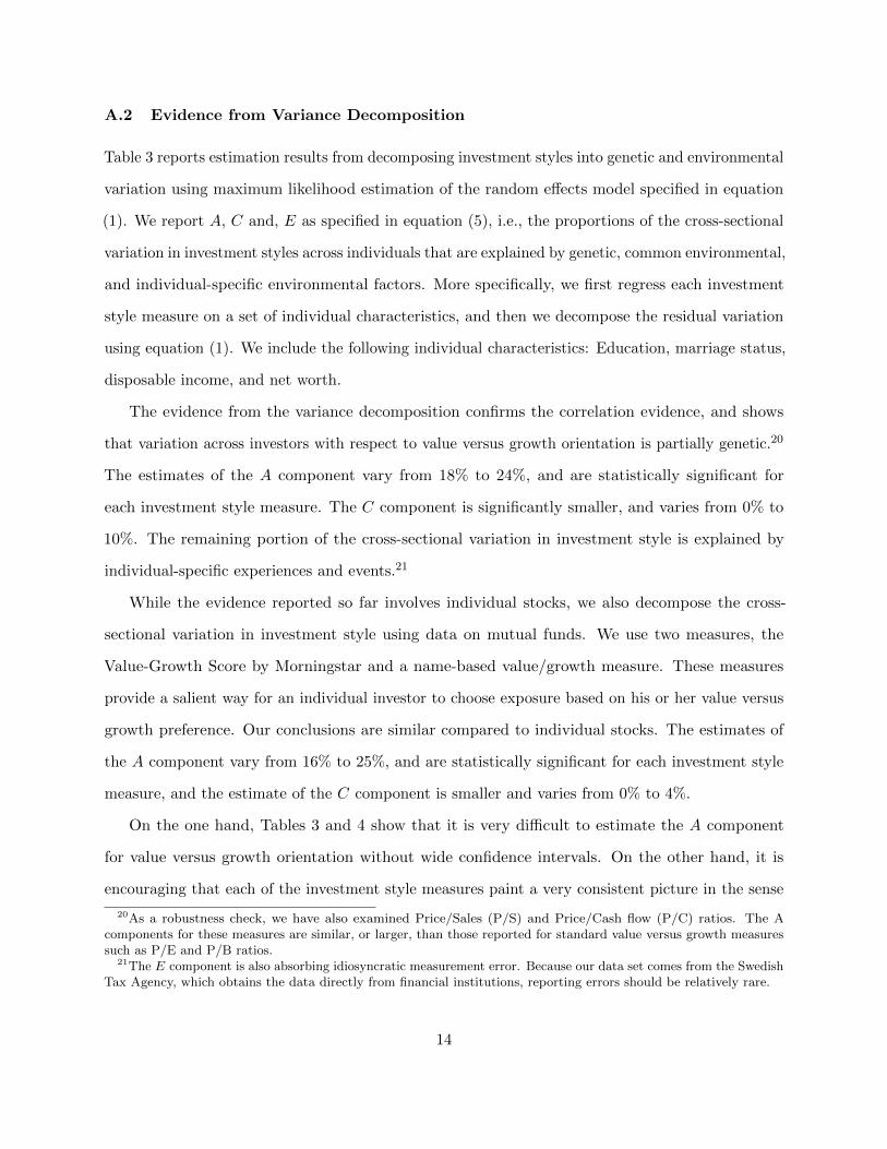
Table 3 reports estimation results from decomposing investment styles into genetic and environmental

variation using maximum likelihood estimation of the random effects model specified in equation

(1). We report A, C and, E as specified in equation (5), i.e., the proportions of the cross-sectional

variation in investment styles across individuals that are explained by genetic, common environmental,

and individual-specific environmental factors. More specifically, we first regress each investment

style measure on a set of individual characteristics, and then we decompose the residual variation

using equation (1). We include the following individual characteristics: Education, marriage status,

disposable income, and net worth.

The evidence from the variance decomposition confirms the correlation evidence, and shows

that variation across investors with respect to value versus growth orientation is partially genetic.20

The estimates of the A component vary from 18% to 24%, and are statistically significant for

each investment style measure. The C component is significantly smaller, and varies from 0% to

10%. The remaining portion of the cross-sectional variation in investment style is explained by

individual-specific experiences and events.21

While the evidence reported so far involves individual stocks, we also decompose the cross-

sectional variation in investment style using data on mutual funds. We use two measures, the

Value-Growth Score by Morningstar and a name-based value/growth measure. These measures

provide a salient way for an individual investor to choose exposure based on his or her value versus

growth preference. Our conclusions are similar compared to individual stocks. The estimates of

the A component vary from 16% to 25%, and are statistically significant for each investment style

measure, and the estimate of the C component is smaller and varies from 0% to 4%.

On the one hand, Tables 3 and 4 show that it is very difficult to estimate the A component

for value versus growth orientation without wide confidence intervals. On the other hand, it is

encouraging that each of the investment style measures paint a very consistent picture in the sense

20As a robustness check, we have also examined Price/Sales (P/S) and Price/Cash flow (P/C) ratios. The Acomponents for these measures are similar, or larger, than those reported for standard value versus growth measuressuch as P/E and P/B ratios.

21The E component is also absorbing idiosyncratic measurement error. Because our data set comes from the SwedishTax Agency, which obtains the data directly from financial institutions, reporting errors should be relatively rare.

14

of a statistically significant A component, for both stocks and mutual funds. It should also be

emphasized that recent studies related to individual investor behavior have had difficulties explaining

even 10% of the cross-sectional variation when including a large set of individual characteristics

(e.g., Brunnermier and Nagel (2008)), so even the lower end of our confidence intervals represent

economically significant effects. Overall, based on the reported evidence, we conclude that an

individual’s investment style has a biological basis, i.e., a preference for value versus growth stocks

is partially ingrained in an investor from birth.

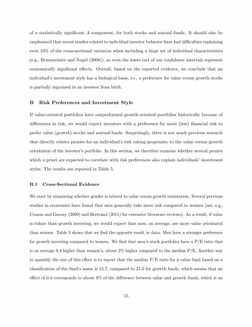
B Risk Preferences and Investment Style

If value-oriented portfolios have outperformed growth-oriented portfolios historically because of

differences in risk, we would expect investors with a preference for more (less) financial risk to

prefer value (growth) stocks and mutual funds. Surprisingly, there is not much previous research

that directly relates proxies for an individual’s risk taking propensity to the value versus growth

orientation of the investor’s portfolio. In this section, we therefore examine whether several proxies

which a priori are expected to correlate with risk preferences also explain individuals’ investment

styles. The results are reported in Table 5.

B.1 Cross-Sectional Evidence

We start by examining whether gender is related to value versus growth orientation. Several previous

studies in economics have found that men generally take more risk compared to women (see, e.g.,

Croson and Gneezy (2009) and Bertrand (2011) for extensive literature reviews). As a result, if value

is riskier than growth investing, we would expect that men, on average, are more value orientated

than women. Table 5 shows that we find the opposite result in data: Men have a stronger preference

for growth investing compared to women. We find that men’s stock portfolios have a P/E ratio that

is on average 0.4 higher than women’s, about 2% higher compared to the median P/E. Another way

to quantify the size of this effect is to report that the median P/E ratio for a value fund based on a

classification of the fund’s name is 15.7, compared to 21.0 for growth funds, which means that an

effect of 0.4 corresponds to about 8% of the difference between value and growth funds, which is an

15

economically significant effect.

We also examine age because older investors are generally found to take less financial risk

compared to younger investors (e.g., Barsky, Juster, Kimball, and Shapiro (1997) and Paulsen et al.

(2012)). A risk preference explanation would predict that older investors are more growth oriented.

Again, Table 5 shows that we find the opposite result in data: Older investors have a significantly

stronger preference for value investing. The average P/E ratio of the stock portfolio of a 65 year old

investor is 4.4 (or about 19% compared to the median) lower compared to a 25 year old.22

We also examine a larger set of proxies potentially related to an individual’s risk taking propensity,

including education, marriage status, disposable income, and net worth. Table 5 first includes these

variables one by one, and then all at the same time. We find that those with a college education

have more growth oriented portfolios compared to lower-education investors, with an average P/E

ratio that is 2.4 (or about 11% compared to the median) higher. Investors who are married and

who have higher disposable incomes and net worth also have a stronger preference for growth. For

example, a one standard deviation change in the log of disposable income corresponds to an average

P/E that is about 1.3 higher.

The overall conclusion from the above analysis is that investors who a priori are expected to

take more financial risk have a preference for growth investing, not value investing. This result

is consistently found in data for both more exogenous variables (e.g., gender and age) and other

individual characteristics.

B.2 Evidence from Discordant Twins

One concern related to the above cross-sectional evidence is that individuals self-select into life

experiences and events partly based on their genetic predispositions. Our specific data enables us

to use a “discordant twin pair research methodology,” which resembles a natural experiment, to

address such concerns. More specifically, this methodology involves comparison of investment styles

within pairs of identical twins, who match on genes and the common environment, but who differ

22Because some studies have found that the very oldest individuals in their samples do take more financial risk (e.g.,Barsky et al. (1997)), we have checked that our conclusion is robust to excluding those over 70 years. Our results areindeed somewhat stronger when we drop the very oldest investors in our data (not tabulated).

16

(i.e., are “discordant”) on other dimensions because of idiosyncratic life experiences.23

We model investment style, sij , for a pair i of identical twins (j = 1, 2) as a function of observable

proxies for individual risk taking propensity Xij and three unobservable effects related to genes and

the common environment, ai, ci, and eij :

yij = β0 + βXij + ai + ci + eij . (6)

By differencing equation (6) within each pair of identical twins we eliminate any effects of genes (ai)

and the common environment (ci):

yi1 − yi2 = β(Xi1 −Xi2) + ei1 − ei2. (7)

If we study the effect of, e.g., education on investment style this methodology enables us to control

for the fact that IQ and cognitive ability is genetic to a significant extent. That is, we are able to

examine the effect of education on value versus growth orientation that is not caused by genetic

differences. The results are reported in Table 6.

We first re-estimate the cross-sectional model for identical twins only to check that the previous

conclusions do not change. Most importantly, the discordant twin pair research methodology shows

that the variables previously included are generally not statistically significant. That is, the effect of

variables such as education and disposable income on investment style appear to be mostly driven

by genetic and common environmental effect.

C Life Course Theory and Investment Style

In this section, we examine to what extent differential life experiences and events of individuals

explain cross-sectional differences in investment styles later in life. Based on pre-existing research in

social psychology we consider several types of potentially relevant, and exogenous, life experiences

of individuals: 1) Macroeconomic experiences, 2) Impressionable years, and 3) Rearing environment.

Table 7 reports the results.

23See Taubman (1976) for an early application of this empirical approach.

17

C.1 Macroeconomic Experiences

We start by examining adverse and significant macroeconomic experiences. First, we analyze

whether there is a pervasive effect on an individual’s investment style of growing up during the

Great Depression. More specifically, we examine the effect on value versus growth orientation of

being born between 1920 and 1929, following the “Depression Baby” definition in Schoar and Zuo

(2013).24 If an adverse macroeconomic experience results in less risk taking later in life, and if

value is riskier than growth investing, we would expect investors who grew up during the Great

Depression to prefer growth investing. An alternative hypothesis, not necessarily based on a risk

explanation, is that those who have more salient experiences of difficult economic conditions develop

a value-oriented investment style, with a preference for relatively “cheaper” stocks. The results in

Panel A of Table 7 are consistent with the latter hypothesis: Individuals who grew up during the

Great Depression show significantly more value-orientation in their stock portfolios several decades

later in life. More specifically, we find that those who grew up during the Great Depression have

portfolios with average P/E ratios that are 2.2 (or about 10% at the median) lower compared to

those of other investors. It is important to emphasize that we control for disposable income and net

worth, which may also be affected by a Great Depression experience.25

Second, we also analyze an individual’s GDP growth experiences during his or her entire life so

far. More specifically, we measure the average GDP growth from an individual’s birth year until

year 2000, i.e., the start of our data set. Experiencing poor GDP growth may reduce an individual’s

propensity to take risk later in life. A risk explanation for investment style would suggest that

individuals with more negative GDP growth experiences become growth investors. An alternative

hypothesis is that experiencing stronger GDP growth results in a growth oriented investment style.

Our results are consistent with the latter hypothesis. We find that for a 100 basis points per year

higher average GDP growth experience during the life, the average P/E ratio of the stock portfolio

24Sweden was affected by the Wall Street Crash of 1929, and was also the origin of the Kreuger Crash of 1932, withadverse international macroeconomic consequences deepening the Depression in several countries, including the U.S.

25The reported “Depression Baby” effect can not be empirically distinguished from a cohort effect unrelated tothe Depression. First, it is not clear what would drive such an effect. One possibility is that those born between1920 and 1929 had parents of similar age who had been affected by macroeconomic experiences, and that the parentstransferred these experiences to their children. Our results are robust to controlling for parents’ age (not tabulated).Second, our results related to impressionable years are not driven by one specific cohort.

18

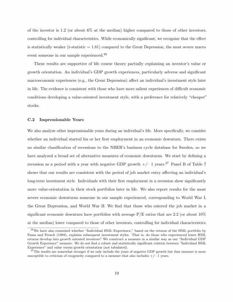
of the investor is 1.2 (or about 6% at the median) higher compared to those of other investors,

controlling for individual characteristics. While economically significant, we recognize that the effect

is statistically weaker (t-statistic = 1.81) compared to the Great Depression, the most severe macro

event someone in our sample experienced.26

These results are supportive of life course theory partially explaining an investor’s value or

growth orientation. An individual’s GDP growth experiences, particularly adverse and significant

macroeconomic experiences (e.g., the Great Depression) affect an individual’s investment style later

in life. The evidence is consistent with those who have more salient experiences of difficult economic

conditions developing a value-oriented investment style, with a preference for relatively “cheaper”

stocks.

C.2 Impressionable Years

We also analyze other impressionable years during an individual’s life. More specifically, we consider

whether an individual started his or her first employment in an economic downturn. There exists

no similar classification of recessions to the NBER’s business cycle database for Sweden, so we

have analyzed a broad set of alternative measures of economic downturns. We start by defining a

recession as a period with a year with negative GDP growth +/– 1 years.27 Panel B of Table 7

shows that our results are consistent with the period of job market entry affecting an individual’s

long-term investment style. Individuals with their first employment in a recession show significantly

more value-orientation in their stock portfolios later in life. We also report results for the most

severe economic downturns someone in our sample experienced, corresponding to World War I,

the Great Depression, and World War II. We find that those who entered the job market in a

significant economic downturn have portfolios with average P/E ratios that are 2.2 (or about 10%

at the median) lower compared to those of other investors, controlling for individual characteristics.

26We have also examined whether “Individual HML Experience,” based on the returns of the HML portfolio byFama and French (1993), explains subsequent investment styles. That is, do those who experienced lower HMLreturns develop into growth oriented investors? We construct a measure in a similar way as our “Individual GDPGrowth Experience” measure. We do not find a robust and statistically significant relation between “Individual HMLExperience” and value versus growth orientation (not tabulated).

27The results are somewhat stronger if we only include the years of negative GDP growth but that measure is moresusceptible to criticism of exogeneity compared to a measure that also includes +/– 1 years.

19

Our result that the preference for value investing among those with their first employment in an

economic downturn is robust to controlling for disposable income and net worth implies that there

is a a direct effect of economic downturns during the impressionable years to investment style later

in life, in addition to any indirect effect on investment style from lower income of those who entered

the job market in economic downturns (e.g., Oreopoulos et al. (2012)). We report similar results if

we examine whether an individual experienced a severe economic downturn when 18-25 years old.

These results are supportive of an impressionable years hypothesis: The economic conditions at

the time of the first job market entry partially explain an individual’s investment style later in life;

the more severe the economic downturn, the more value oriented the individual is later on.

C.3 Rearing Environment

We also examine whether the rearing environment has significant long-term effects on an individual’s

investment style later in life. First, we examine the socioeconomic status (SES) of an individual’s

parents. We are not able to measure parents’ SES exactly when an individual grew up, so we use

parents’ net worth at the start of our data set as a proxy. The results are reported in Panel C of

Table 7. We find that individuals who grew up in a lower SES environment, i.e., relatively poor,

show significantly more value-orientation in their stock portfolios later in their lives. Investors at

the bottom of the parental wealth distribution (10th percentile) have portfolios with average P/E

ratios that are 1.0 (or about 5% at the median) lower compared to investors at the top of the

distribution (90th percentile). We show that this effect is robust also within each generation by

controlling for birth cohort (decade) fixed effects, i.e., this result is not specific only to the Great

Depression cohort. Second, we examine whether parents’ life experiences transfer to their children

and affect the investment style also of the next generation. We find evidence consistent with an

inter-generational transfer of parental life experiences. Investors whose parents were born between

1920 and 1929, i.e., grew up during the Great Depression, show significantly more value orientation.

Comparing the Great Depression effect on an individual’s own investment style to the one of the

next generation we find that about half of the effect is transmitted to the children.

The overall conclusion from the above analysis is that individuals’ investment styles are affected

20

also by the rearing environment in which they grew up, in particular their parents’ socio-economic

status and their parents’ life experiences.

VI Discussion

In this section, we discuss some of the potential implications of our results.

Mechanisms? While our study shows that an individual’s investment style is explained by both

biological predispositions as well as experiences and events during the course of life, it is silent on

the specific mechanisms than explain these effects. Using gene candidate studies or genome-wide

association studies (GWAS) to identify the specific set of gene(s) that explain value versus growth

orientation would be a natural next step. As the number of studies in economics and finance that

support life course theory and an impressionable years hypothesis increases, another necessary next

step is to uncover the mechanisms than explain why macroeconomic and other events are related to

investment behavior decades later. For example, recent research on neurological development shows

that, in the developing brain, the volume of gray matter in the cortex gradually increases until about

the age of adolescence, but then sharply decreases as the brain prunes away neuronal connections

that are deemed superfluous to the adult needs of the individual (e.g., Spear (2000)). Such evidence

may provide a mechanism for early life experiences explaining an individual’s investment behavior

later in life, but more research is required.

Asset prices and the value premium? First, our results imply that the overall genetic composition

in a market may affect the demand for value versus growth stocks, and in the end potentially

equilibrium asset prices. In markets where the genes explaining a value preference are relatively

more prevalent, we may expect stronger demand for value stocks, and as a result a relatively smaller

equilibrium value premium (if the supply of value and growth stocks is not responding perfectly).

Once the specific genes involved in explaining a value preference have been identified, researchers

may analyze whether the relative prevalence of these genes in different markets affect the value

premium in these markets. Second, our result that gender and age are related to value versus

growth orientation implies that the the gender distribution and the age distribution in a market

may partially explain the value premium. Markets with significant gender or age imbalances may

21

provide researchers with opportunities to analyze this implication. Finally, the life experiences

of the participants in a particular market may affect the demand for value versus growth stocks,

potentially resulting in “legacy effects” of macro events that occurred a long time ago also for the

value premium, similar to the implications of Friedman and Schwartz (1963) and Cogley and Sargent

(2008) for the equity premium.

Inefficiency of investor portfolios? The finding that value stocks historically have outperformed

growth portfolios is explained by risk in standard finance models. Casual evidence suggests that

many individual investors do not seem to perceive value as riskier than growth portfolios. Many

mutual fund companies also seem to promote this view. To provide only one examples, Fidelity

explains the difference between value and growth funds to investors as follows on their website:

“While growth funds are expected to offer the potential for higher returns, they also generally

represent a greater risk when compared to value funds.”28 We find that investors who a priori are

expected to take more financial risk have a preference for growth, not value, investing. If value

actually is riskier than growth, for example because asset prices are set by institutional investors,

individuals’ mis-calibration imply that value (growth) investors may take significantly more (less)

risk than they would have done if they were appropriately calibrated. As a consequence, many

investors may end up with inefficient portfolios.

VII Conclusion

We report that several factors explain an investor’s style, i.e., the value versus growth orientation

of the investor’s stock portfolio. First, an investor’s style has a biological basis – a preference for

value versus growth stocks is partially ingrained in an investor already from birth. We estimate

that genetic differences across individuals explain 18% of the cross-sectional variation in value

versus growth orientation, if using P/E ratios as an investment style measure, and 25% if using

Morningstar’s Value-Growth Score. This evidence contributes to a growing number of studies which

show that individual characteristics of importance for portfolio choice are partly explained by an

individual’s biological predispositions and genetic composition (e.g., Cesarini et al. (2009), Kuhnen

28https://www.fidelity.com/learning-center/mutual-funds/growth-vs-value-investing.

22

and Chiao (2009), and Barnea, Cronqvist, and Siegel (2010)).

Second, investors who a priori are expected to take more financial risk have a preference for

growth, not value, investing. This result is consistently found in data for exogenous proxies for risk

taking propensity (e.g., gender and age) and also other individual characteristics (e.g., wealth). If

value is riskier than growth, it may be surprising that those who are expected to take more (less)

financial risk prefer growth (value) stock portfolios. This evidence suggests that either value is

not riskier than growth, or that the average individual investor in mis-calibrated about the risk

of value versus growth investing. In this sense, our research contributes a new perspective to the

long-standing value/growth debate in finance (e.g., Fama and French (1992, 1993) Lakonishok,

Shleifer, and Vishny (1994)). More specifically, we provide a new perspective on the source of the

value premium by showing that individual investors’ portfolio choices do not seem to be consistent

with a risk explanation.

Finally, an investor’s style is explained by life course theory in that experiences, both earlier and

later in life, are related to investment style. In particular, investors with adverse macroeconomic

experiences have stronger preferences for value investing later in life. For example, those who grew

up during the Great Depression have portfolios with average P/E ratios that are 2.2 (or about

10% at the median) lower, controlling for individual characteristics, several decades later in life.

Consistent with an impressionable years hypothesis, those who enter the job market for the first

time during an economic downturn are also more value oriented later on. We also find that those

who grew up in a lower status socio-economic rearing environment have a stronger value orientation

later in life. This evidence contributes to several recent studies which show the importance of life

experiences and events for economic behaviors later in life (e.g., Oyer (2006), Kaustia and Knupfer

(2008), Malmendier and Nagel (2011), and Giuliano and Spilimbergo (2013)).

23

References

Alesina, A., Fuchs-Schuendeln, N., 2005. Good bye Lenin (or not?): The effect of Communism onpeople’s preferences. American Economic Review 97, 1507–1528.

Almond, D., Currie, J., 2011. Killing me softly: The fetal origins hypothesis. Journal of EconomicPerspectives 25 (3), 153–172.

Ashenfelter, O., Krueger, A. B., 1994. Estimates of the economic returns to schooling from a newsample of twins. American Economic Review 84 (5), 1157–1173.

Barberis, N., Shleifer, A., 2003. Style investing. Journal of Financial Economics 68 (2), 161–199.

Barberis, N., Shleifer, A., Vishny, R. W., 1998. A model of investor sentiment. Journal of FinancialEconomics 49, 307–343.

Barnea, A., Cronqvist, H., Siegel, S., 2010. Nature or nurture: What determines investor behavior?Journal of Financial Economics 98, 583–604.

Barsky, R. B., Juster, F. T., Kimball, M. S., Shapiro, M. D., 1997. Preference parameters andbehavioral heterogeneity: An experimental approach in the health and retirement study. QuarterlyJournal of Economics 112, 537–579.

Behrman, J. R., Taubman, P., 1976. Intergenerational transmission of income and wealth. AmericanEconomic Review 66, 436–440.

Behrman, J. R., Taubman, P., 1989. Is schooling “mostly in the genes”? Nature-nurture decomposi-tion using data on relatives. Journal of Political Economy 97, 1425–1446.

Bertrand, M., 2011. New perspectives on gender. Handbook of Labor Economics 4, 1543–1590.

Bisin, A., Verdier, T., 2000. Beyond the melting pot: Cultural transmission, marriage, and theevolution of ethnic and religious traits. Quarterly Journal of Economics 115 (3), 955–988.

Bisin, A., Verdier, T., 2001. The economics of cultural transmission and the dynamics of preferences.Journal of Economic Theory 97 (2), 298 – 319.

Black, S. E., Devereux, P. J., Salvanes, K. G., 2005. The more the merrier? The effect of family sizeand birth order on children’s education. Quarterly Journal of Economics 120 (2), 669–700.

Black, S. E., Devereux, P. J., Salvanes, K. G., 2007. From the cradle to the labor market? Theeffect of birth weight on adult outcomes. Quarterly Journal of Economics 122 (1), 409–439.

Brennan, T. J., Lo, A. W., 2011. The origin of behavior. Quarterly Journal of Finance 1, 55–108.

Brunnermier, M. K., Nagel, S., 2008. Do wealth fluctuations generate time-varying risk aversion?Micro-evidence on individuals’ asset allocation. American Economic Review 98, 713–736.

Carlen, J., 2012. Einstein of Money: The Life and Timeless Financial Wisdom of Benjamin Graham.Prometheus Books.

24

Cesarini, D., Dawes, C. T., Johannesson, M., Lichtenstein, P., Wallace, B., 2009. Genetic variationin preferences for giving and risk taking. Quarterly Journal of Economics 124, 809–842.

Cesarini, D., Johannesson, M., Lichtenstein, P., Sandewall, O., Wallace, B., 2010. Genetic variationin financial decision making. Journal of Finance 65, 1725–1754.

Cesarini, D., Johannesson, M., Magnusson, P. K. E., Wallace, B., 2012. The behavioral genetics ofbehavioral anomalies. Management Science 58, 21–34.

Chan, L. K. C., Hamao, Y., Lakonishok, J., 1991. Fundamentals and stock returns in Japan. Journalof Finance 46 (5), 1739–1764.

Chan, L. K. C., Lakonishok, J., 2004. Value and growth investing: Review and update. FinancialAnalysts Journal, 71–86.

Chen, M. K., Lakshminarayanan, V., Santos, L. R., 2006. How basic are behavioral biases? Evidencefrom Capuchin monkey trading behavior. Journal of Political Economy 114 (3), 517–537.

Chetty, R., Friedman, J. N., Hilger, N., Saez, E., Schanzenbach, D. W., Yagan, D., 2011. Howdoes your kindergarten classroom affect your earnings? Evidence from Project STAR. QuarterlyJournal of Economics 126 (4), 1593–1660.

Cogley, T., Sargent, T. J., 2008. The market price of risk and the equity premium: A legacy of theGreat Depression? Journal of Monetary Economics 55 (3), 454–476.

Cosmides, L., Tooby, J., 1994. Better than rational: Evolutionary psychology and the invisible hand.American Economic Review 84 (2), 327–332.

Cronqvist, H., Previtero, A., Siegel, S., White, R. E., 2013. Prenatal exposure to testosteroneincreases financial risk-taking and reduces the gender gap. Working paper, University of WesternOntario, Richard Ivey School of Business.

Cronqvist, H., Siegel, S., 2013. The genetics of investment biases. Forthcoming Journal of FinancialEconomics.

Croson, R., Gneezy, U., 2009. Gender differences in preferences. Journal of Economic Literature 47,1–27.

Currie, J., 2011. Inequality at birth: Some causes and consequences. American Economic Review101 (3), 1–22.

Daniel, K., Hirshleifer, D., Subrahmanyam, A., 1998. Investor psychology and security marketunder-and overreactions. Journal of Finance 53 (6), 1839–1885.

Daniel, K., Titman, S., 1997. Evidence on the characteristics of cross sectional variation in stockreturns. Journal of Finance 52 (1), 1–33.

Daniel, K., Titman, S., Wei, K., 2001. Explaining the cross-section of stock returns in Japan: Factorsor characteristics? Journal of Finance 56 (2), 743–766.

De Bondt, W. F. M., Thaler, R. H., 1985. Does the stock market overreact? Journal of Finance 40,793–805.

25

De Long, J. B., Shleifer, A., Summers, L. H., Waldmann, R. J., 1990. Positive feedback investmentstrategies and destabilizing rational speculation. Journal of Finance 45 (2), 379–395, english.

Dreber, A., Apicella, C. L., Eisenberg, D. T. A., Garcia, J. R., Zamore, R. S., 2009. The 7Rpolymorphism in the dopamine receptor D4 gene (DRD4) is associated with financial risk-takingin men. Evolution and Human Behavior 30, 85–92.

Elder, G. H., 1974. Children of the Great Depression: Social Change in Life Experience. Universityof Chicago Press.

Elder, G. H., Johnson, M. K., Crosnoe, R., 2003. The emergence and development of life coursetheory. Kluwer Academic Publishers, pp. 3–19.

Falconer, D. S., Mackay, T. F. C., 1996. Introduction to quantitative genetics, 4th Edition.

Fama, E. F., French, K. R., 1992. The cross-section of expected stock returns. Journal of Finance47 (2), 427–465.

Fama, E. F., French, K. R., 1993. Common risk factors in the returns on stocks and bonds. Journalof Financial Economics 33 (1), 3–56.

Fama, E. F., French, K. R., 1996. Multifactor explanations of asset pricing anomalies. Journal ofFinance 51 (1), 55–84.

Fama, E. F., French, K. R., 1998. Value versus growth: The international evidence. Journal ofFinance 53 (6), 1975–1999.

Friedman, M., Schwartz, A. J., 1963. A Monetary History of the United States, 1867-1960. PrincetonUniversity Press.

Giele, J. Z., Elder, G. H., 1998. Methods of life course research: Qualitative and quantitativeapproaches. Sage Publications.

Giuliano, P., Spilimbergo, A., 2013. Growing up in a recession. Forthcoming Review of EconomicStudies.

Grinblatt, M., Keloharju, M., 2009. Sensation seeking, overconfidence, and trading activity. Journalof Finance 64, 549–578.

Hong, H., Stein, J. C., 1999. A unified theory of underreaction, momentum trading, and overreactionin assets markets. Journal of Finance 54 (6), 2143–2184.

Kaustia, M., Knupfer, S., 2008. Do investors overweight personal experience? Evidence from IPOsubscriptions. Journal of Finance 63 (6), 2679–2702.

Krosnick, J. A., Alwin, D. F., 1989. Aging and susceptibility to attitude change. Journal of Personalityand Social Psychology 57 (3), 416.

Kuhnen, C. M., Chiao, J., 2009. Genetic determinants of financial risk taking. PLoS ONE 4.

Lakonishok, J., Shleifer, A., Vishny, R. W., 1994. Contrarian investment, extrapolation, and risk.Journal of Finance 49 (5), 1541–1578.

26

Lichtenstein, P., Sullivan, P. F., Cnattingius, S., Gatz, M., Johansson, S., Carlstrom, E., Bjork, C.,Svartengren, M., Wolk, A., Klareskog, L., de Faire, U., Schalling, M., Palmgren, J., Pedersen,N. L., 2006. The Swedish twin registry in the third millennium: An update. Twin Research andHuman Genetics 9, 875–882.

Malmendier, U., Nagel, S., 2011. Depression babies: Do macroeconomic experiences affect risk-taking? Quarterly Journal of Economics 126 (1), 373–416.

Malmendier, U., Nagel, S., 2013. Learning from inflation experiences. Working paper, NBER.

Malmendier, U., Tate, G., Yan, J., 2011. Overconfidence and early-life experiences: The effect ofmanagerial traits on corporate financial policies. Journal of Finance 66 (5), 1687–1733.

Merton, R. C., 1969. Lifetime portfolio selection under uncertainty: The continuous-time case.Review of Economics and Statistic 51, 247–257.

Oreopoulos, P., von Wachter, T., Heisz, A., 2012. The short-and long-term career effects of graduatingin a recession. American Economic Journal: Applied Economics 4 (1), 1–29.

Oyer, P., 2006. Initial labor market conditions and long-term outcomes for economists. Journal ofEconomic Perspectives 20, 143–160.

Oyer, P., 2008. The making of an investment banker: Stock market shocks, career choice, andlifetime income. Journal of Finance 63 (6), 2601–2628.

Paulsen, D. J., Platt, M. L., Huettel, S. A., Brannon, E. M., 2012. From risk-seeking to risk-averse:The development of economic risk preference from childhood to adulthood. Frontiers in Psychology3.

Rayo, L., Becker, G., 2007. Evolutionary efficiency and happiness. Journal of Political Economy115 (2).

Robson, A. J., 2001a. The biological basis of economic behavior. Journal of Economic Literature 29,11–33.

Robson, A. J., 2001b. Why would nature give individuals utility functions? Journal of PoliticalEconomy 109, 900–914.

Samuelson, P. A., 1969. Lifetime portfolio selection by dynamic stochastic programming. Review ofEconomics and Statistics 51, 239–246.

Santos, L. R., Chen, M. K., 2009. The evolution of rational and irrational economic behavior:Evidence and insight from a non-human primate species. In: Glimcher, P., Camerer, C., Fehr, E.,Poldrack, R. (Eds.), Neuroeconomics: Decision-Making and the Brain. Elsevier, London, U.K.,pp. 81–94.

Schoar, A., Zuo, L., 2013. Shaped by booms and busts: How the economy impacts CEO careers andmanagement styles. Working paper, MIT Sloan School of Management.

Spear, D. O., 2000. Neurobehavioral changes in adolescence. Current Directions in PsychologicalScience 9, 111–114.

27

Taubman, P., 1976. The determinants of earnings: Genetics, family, and other environments; Astudy of white male twins. American Economic Review 66 (5), 858–870.

Zhong, S., Israel, S., Xue, H., Ebstein, R. P., Chew, S. H., 2009. Monoamine Oxidase A gene(MAOA) associated with attitude towards longshot risks. PLoS ONE 4.

28

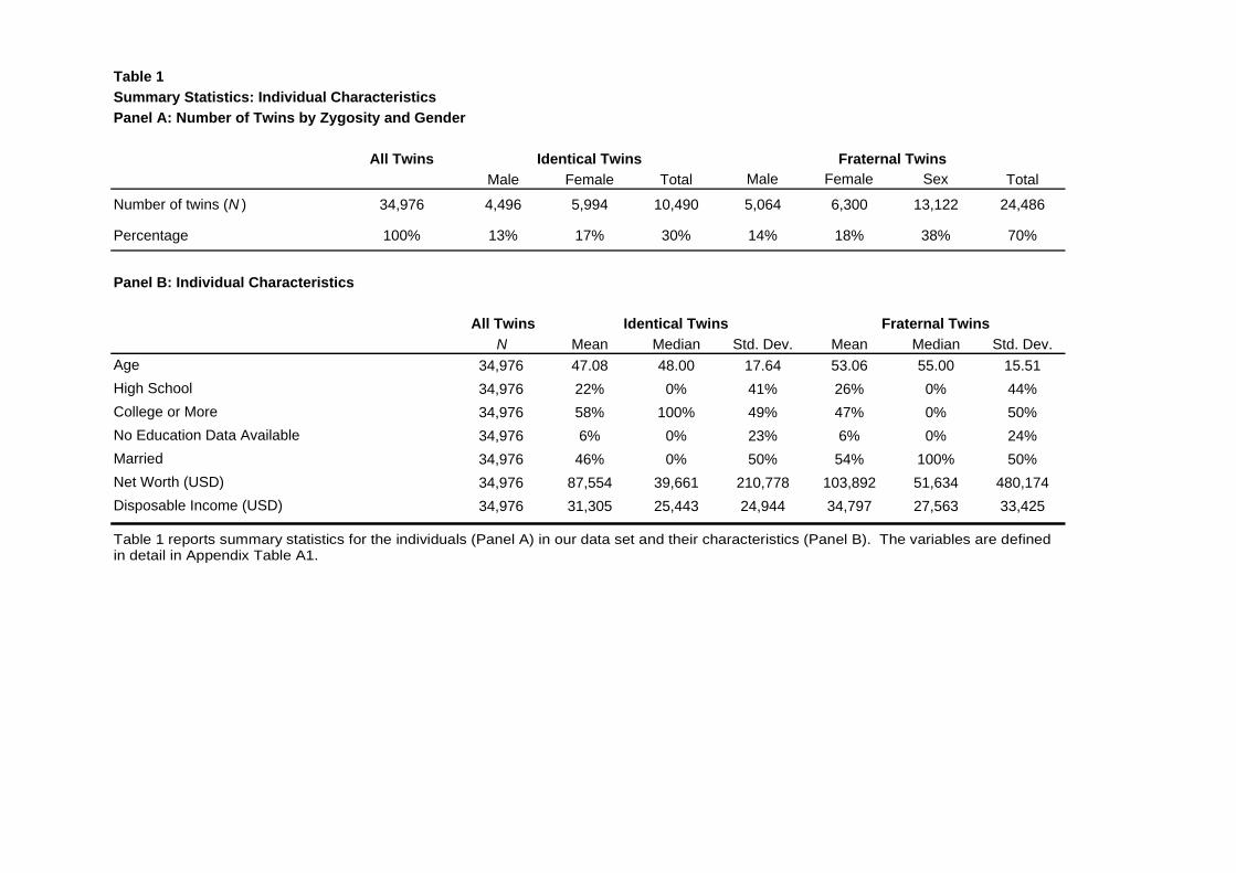
Table 1Summary Statistics: Individual CharacteristicsPanel A: Number of Twins by Zygosity and Gender

All TwinsMale Female Total Male Female Sex Total

Number of twins (N ) 34,976 4,496 5,994 10,490 5,064 6,300 13,122 24,486

Percentage 100% 13% 17% 30% 14% 18% 38% 70%

Panel B: Individual Characteristics

All TwinsN Mean Median Std. Dev. Mean Median Std. Dev.

34,976 47.08 48.00 17.64 53.06 55.00 15.5134,976 22% 0% 41% 26% 0% 44%34,976 58% 100% 49% 47% 0% 50%34,976 6% 0% 23% 6% 0% 24%34,976 46% 0% 50% 54% 100% 50%34,976 87,554 39,661 210,778 103,892 51,634 480,17434,976 31,305 25,443 24,944 34,797 27,563 33,425

No Education Data AvailableMarriedNet Worth (USD)Disposable Income (USD)

College or MoreHigh SchoolAge

Identical Twins Fraternal Twins

Identical Twins Fraternal Twins

Table 1 reports summary statistics for the individuals (Panel A) in our data set and their characteristics (Panel B). The variables are defined in detail in Appendix Table A1.

Table 2Summary Statistics: Investment Style Measures

N Mean Median Std. Dev. Mean Median Std. Dev.Stocks P/E 17,952 24.2 22.8 14.6 23.0 21.3 13.1P/B 18,337 3.3 2.8 2.4 3.2 2.5 2.3Mutual FundsMorningstar's Value-Growth Score 25,729 156.4 149.2 21.4 155.2 148.6 21.0Name-Based Value/Growth Measure 27,397 0.1 149.2 0.2 0.1 0.0 0.2

Identical Twins Fraternal Twins

Table 2 reports summary statistics for the measures of investment style. The variables are defined in detail in Appendix Table A1.

Table 3Evidence from Variance Decomposition of Investment Style: Stocks

P/E P/BA Share 0.181** 0.241**

0.076 0.118C Share 0.101* 0.080

0.056 0.096E Share 0.718*** 0.679***

0.030 0.046Individual Characteristics Included Yes YesN 10,618 10,640Table 3 reports results from maximum likelihood estimation. The different investment style measures are modeled as linear functions of observable individual characteristics and unobservable random effects representing additive genetic effects (A), shared environmental effects (C), as well as an individual-specific error (E). For each estimated model, we report the variance fraction of the residual explained by each unobserved effect (A Share – for the additive genetic effect, C Share – for common environmental effect, E Share – for the individual-specific environmental effect) as well as the bootstrapped standard errors (1,000 resamples). The variables are defined in detail in Appendix Table A1.

Table 4Evidence from Variance Decomposition of Investment Style: Mutual Funds

Morningstar's Value-Growth Score Name-Based Value/Growth MeasureA Share 0.249*** 0.159**

0.026 0.065C Share 0.000 0.036

0.009 0.040E Share 0.751*** 0.805***

0.022 0.031Individual Characteristics Included Yes YesN 17,534 17,650

Table 4 reports results from maximum likelihood estimation. The different investment style measures are modeled as linear functions of observable individual characteristics and unobservable random effects representing additive genetic effects (A), shared environmental effects (C), as well as an individual-specific error (E). For each estimated model, we report the variance fraction of the residual explained by each unobserved effect (A Share – for the additive genetic effect, C Share – for common environmental effect, E Share – for the individual-specific environmental effect) as well as the bootstrapped standard errors (1,000 resamples). The variables are defined in detail in Appendix Table A1.

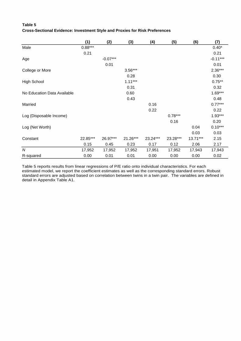
Table 5Cross-Sectional Evidence: Investment Style and Proxies for Risk Preferences

(1) (2) (3) (4) (5) (6) (7)Male 0.88*** 0.40*

0.21 0.21Age -0.07*** -0.11***

0.01 0.01College or More 3.56*** 2.36***

0.28 0.30High School 1.11*** 0.75**

0.31 0.32No Education Data Available 0.60 1.69***

0.43 0.48Married 0.16 0.77***

0.22 0.22Log (Disposable Income) 0.78*** 1.93***

0.16 0.20Log (Net Worth) 0.04 0.10***

0.03 0.03Constant 22.85*** 26.97*** 21.26*** 23.24*** 23.28*** 13.71*** 2.15

0.15 0.45 0.23 0.17 0.12 2.06 2.17N 17,952 17,952 17,952 17,951 17,952 17,943 17,943R-squared 0.00 0.01 0.01 0.00 0.00 0.00 0.02

Table 5 reports results from linear regressions of P/E ratio onto individual characteristics. For each estimated model, we report the coefficient estimates as well as the corresponding standard errors. Robust standard errors are adjusted based on correlation between twins in a twin pair. The variables are defined in detail in Appendix Table A1.

Table 6Evidence from Discordant Twins: Investment Style and Proxies for Risk Preferences

Cross-Section Discordant TwinsMale 1.59***

0.44Age -0.12***

0.02College or More 1.77*** 2.86

0.66 1.76High School 0.23 2.39

0.70 1.51No Education Data Available 1.50 3.81

0.99 2.85Married 1.12** -0.22

0.44 0.68Log (Disposable Income) 1.73*** 0.61

0.40 0.68Log (Net Worth) 0.07 0.21

0.07 0.13Constant 5.54 -0.21

4.39 0.39N 5,201 1,877R-squared 0.02 0.01

Table 6 reports results from linear regressions of P/E ratio (column “Cross-Section”) onto individual characteristics, and intra twin-pair difference in the P/E ratio on differences in individual characteristics (column “Discordant Twins”). For each estimated model, we report the coefficient estimates as well as the corresponding standard errors. Robust standard errors are adjusted based on correlation between twins in a twin pair. The variables are defined in detail in Appendix Table A1.

Table 7Life Course Theory and Investment Style

Panel A: Macroeconomic Experiences

(1) (2)Depression Baby -2.17***

0.53Individual GDP Growth Experience 1.23*

0.68Constant 2.12 -0.48

2.17 2.61Individual Characteristics Included Yes YesN 17,943 17,943R-squared 0.02 0.02

Panel B: Impressionable Years

(1) (2) (3)First Job in Recession -0.78**

-0.35First Job in Severe Recession -2.18***

0.5718-25 Years Old in Severe Recession -3.83***

0.71Constant 3.73 3.87* 3.86*

2.32 2.32 2.31Individual Characteristics Included Yes Yes Yes

Table 7 reports results from linear regressions of P/E ratio onto macroeconomic experience variables (Panel A), impressionable years variables (Panel B), and rearing environment variables (Panel C). For each estimated model, we report the coefficient estimates as well as the corresponding standard errors. Robust standard errors are adjusted based on correlation between twins in a twin pair. The variables are defined in detail in Appendix Table A1.

N 16,462 16,462 16,462R-squared 0.02 0.02 0.02

Panel C: Rearing Environment

(1) (2) (3) (4)Log (Parents' Net Worth) 0.26** 0.27** 0.30*** 0.30***

0.11 0.11 0.11 0.11Depression Baby Parents -1.33*** -1.20**

0.47 0.5Constant 5.12 4.94 4.74 4.69

3.59 4.73 3.59 4.73Individual Characteristics Included Yes Yes Yes YesBirth Cohort (Decade) Fixed Effects No Yes No YesN 8,101 8,101 8,101 8,101R-squared 0.02 0.02 0.02 0.02

Table 7 reports results from linear regressions of P/E ratio onto macroeconomic experience variables (Panel A), impressionable years variables (Panel B), and rearing environment variables (Panel C). For each estimated model, we report the coefficient estimates as well as the corresponding standard errors. Robust standard errors are adjusted based on correlation between twins in a twin pair. The variables are defined in detail in Appendix Table A1.

Appendix Table A1Variable Definitions

Category / Variable Description

Individual CharacteristicsMale An indicator variable that equals 1 if an individual is male, and 0 otherwise. DataAge Average age across the years an individual is in the data set. Data from Statistics

Sweden.College or More An indicator variable that equals 1 if an individual has attended university, and 0

otherwise. Data from Statistics Sweden.High School An indicator variable that equals 1 if an individual has completed high school

("gymnasium"), and 0 otherwise. Data from Statistics Sweden.No Education Data Available An indicator variable that equals 1 if no educational data are available for an

individual, and 0 otherwise. Data from Statistics Sweden.Married Average of an annual indicator variable that equals 1 if an individual is married, and

0 otherwise. Averaged across those years an individual is in the data set. Datafrom Statistics Sweden.

Disposable Income Average individual disposable income, i.e., the sum of income from labor,business, and investment, plus received transfers, less taxes, and alimonypayments. Averaged across those years an individual is in the data set.Expressed in nominal Swedish Krona (SEK). Data from Statistics Sweden.

Net Worth Average difference between the end-of-year market value of an individual's assetsand liabilities. Averaged across those years an individual is in the data set.Expressed in nominal Swedish Krona (SEK). Data from Statistics Sweden.

Investment StyleP/E The value-weighted price to earnings ratio for each year, averaged across those

years an individual is in the data set. Data from CapitalIQ.P/B The value-weighted market value to book value of equity ratio for each year,

averaged across those years an individual is in the data set. Data from CapitalIQ.Morningstar's Value-Growth Score Morningstar's score of value/growth from -100 (value) to +400 (growth). The

variable is value-weighted for each year and averaged across those years anindividual is in the data set.

Name-based Value/Growth Measure A variable that equals -1 if a fund's name contains "value," equals +1 if a fund'sname contains "growth" or "high tech," and zero otherwise. The variable is value-weighted for each year and averaged across those years an individual is in the data

Experience and EventsDepression Baby An indicator variable that equals 1 if a individual was born 1920-1929, and

otherwise 0.Individual GDP Growth Experience The average of GDP growth in Sweden from an individual's birth to year 2000.First Job in Recession A "Recession Year" is a year with negative GDP growth. The variable is an

indicator variable that equals 1 if an individual entered the job market for the firsttime during a recession year +/- 1 year, and 0 otherwise.

First Job in Severe Recession The variable is an indicator variable that equals 1 if an individual entered the jobmarket for the first time during World War I, the Great Depression, or World War II,and 0 otherwise.

Parents' Net Worth An individual's parents' net worth.Depression Baby Parents An indicator variable that equals 1 if both parents of an individual were born 1920-

1929, and 0 otherwise.

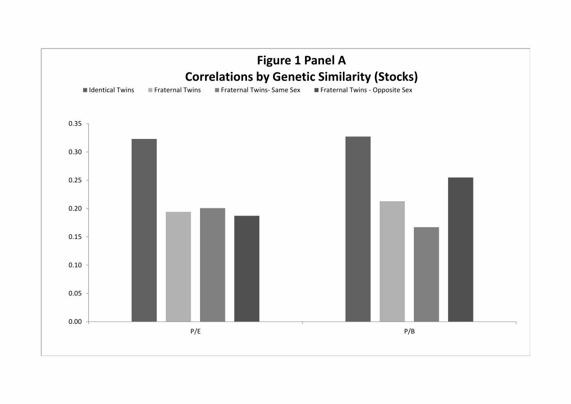
0.00

0.05

0.10

0.15

0.20

0.25

0.30

0.35

P/E P/B

Figure 1 Panel ACorrelations by Genetic Similarity (Stocks)

Identical Twins Fraternal Twins Fraternal Twins‐ Same Sex Fraternal Twins ‐ Opposite Sex

0.00

0.05

0.10

0.15

0.20

0.25

0.30

Morningstar's Value‐Growth Score Name‐Based Value/Growth Measure

Figure 1 Panel BCorrelations by Genetic Similarity (Mutual Funds)

Identical Twins Fraternal Twin Fraternal Twins‐Same Sex Fraternal Twins‐Opposite Sex