valuing convertible bonds: a new approach · 2018-12-27 · requires a contingent claims valuation...

Valuing Convertible Bonds: A New Approach

John D. Finnerty, PhD, and Mengyi Tu

John D. Finnerty is a Professor of Finance at Fordham University’s Gabelli School of Business and an AcademicAffiliate of AlixPartners LLP. Mengyi Tu is an Associate of AlixPartners LLP.

A recent paper by Finnerty expresses the value of a convertible bond as the value of

the straight bond component plus the value of the option to exchange the bond

component for a specified number of conversion shares and develops a closed-form

convertible bond valuation model. This article illustrates how to apply the model to

value nonredeemable convertible bonds and callable convertible bonds. The article

also compares model and market prices for a sample of 148 corporate convertible

bonds issued between 2006 and 2010. The average median and mean pricing errors

are�0.18% and 0.21%, respectively, which are within the average bid-ask spread for

convertible bonds during the postcrisis sample period.

Introduction

A convertible bond gives the holder an American

option to convert the bond into common stock by

exchanging it for a specified number of common shares

at any time prior to the bond’s redemption. Often, the firm

has an American call option, which it can use to force

conversion before the bondholders voluntarily convert, if

the conversion option is in-the-money, and the bond-

holders may have one or more European put options,

which they can use to force premature redemption. The

interaction of these options with the firm’s default option

requires a contingent claims valuation model to capture

fully a convertible bond’s complex optionality.

A recent article by Finnerty (2015) models an

investor’s option to exchange the straight bond compo-

nent for the conversion shares and develops a closed-form

convertible bond valuation model. It obtains an explicit

expression for the value of the option to exchange the

straight bond for the conversion shares by applying

Margrabe’s (1978) insight into how to value the option to

exchange one asset for another asset. It then expresses the

value of a convertible bond as the value of the straight

bond component plus the value of the exchange option

component.

This article illustrates how to apply the model to value

nonredeemable convertible bonds and callable convert-

ible bonds. It values callable convertibles by modeling the

firm’s option to force early conversion within a stopping

time framework. The exchange option convertible bond

pricing model is simpler to use than the more mathemat-

ically sophisticated partial differential equation (PDE)

models. The article also reports the results of empirical

tests of the model. The overall average median and mean

pricing errors are�0.18% and 0.21%, respectively, which

are within the average bid-ask spread for the convertible

bond sample during the postcrisis period.

Literature Review

The convertible securities literature reflects two main

strands of research. One set of papers (Lewis, Rogalski,

and Seward 1998; Lewis and Verwijmeren 2011; Nyborg

1996) investigates how the traditional convertible bond

structure—straight bond with the option to convert it into

a fixed number of common shares—has been reengi-

neered.1 These papers analyze the firm’s motivation for

developing innovative structures, including the desire to

mitigate the costs of external financing, such as asset

substitution (Green 1984), financial distress and asym-

metric information (Brown et al. 2011; Nyborg 1995;

Stein 1992), risk uncertainty (Brennan and Schwartz

1988), and over-investment (Mayers 1988); to give

conventional bond investors an equity sweetener (Nyborg

1996); and to manage publicly reported earnings (Lewis

and Verwijmeren 2011). The literature has documented a

rich variety of innovative structures (Bhattacharya 2012;

Lewis and Verwijmeren 2011).

Convertible securities have evolved in response to the

capital market’s growing sophistication and improved

analytical capability. The optionality of convertible

securities is attractive to hedge funds, which accounted

1 The conversion price is usually, but not always, fixed. For example,Hillion and Vermaelen (2004) describe a class of floating priceconvertible securities, which smaller high-risk firms have issued.

Business Valuation ReviewTM — Fall 2017 Page 85

Business Valuation Reviewe

Volume 36 � Number 3

� 2017, American Society of Appraisers

for about 80% of the funds invested in convertible

securities in the United States and possibly an even higher

percentage of European convertibles prior to the recent

financial crisis (Bhattacharya 2012; Horne and Dialynas

2012).2 Hedge funds, in particular, develop arbitrage

strategies that are designed to capitalize on the perceived

mispricing of the convertibles’ embedded options.3 This

article concerns the traditional form of callable convert-

ible bond, which again accounts for the majority of new

issuance as hedge funds have become less of an influence

since the 2008–2009 financial crisis (Bhattacharya 2012).

The second main body of convertible securities

research develops and empirically tests convertible

security pricing models. Contingent claims models for

convertible bond pricing first appeared in the 1970s.

Ingersoll (1977) and Brennan and Schwartz (1977)

developed the first such models in the spirit of the

seminal Black-Scholes-Merton (Black and Scholes 1973;

Merton 1973) contingent claims methodology. They

develop PDE models, which specify a stochastic process

for each factor that drives option value, correlations

between processes, and a set of boundary conditions that

embody the assumed option exercise behavior. Ingersoll

(1977) and Brennan and Schwartz (1977) develop single-

factor structural models that extend Merton’s (1974)

corporate bond valuation model to convertible bonds. The

value of the firm’s assets follows geometric Brownian

motion, and the firm’s equity, convertible securities, and

other debt are contingent claims on the value of its assets.

Debt holders face credit risk because they get fully paid

only if the value of the firm’s assets exceeds what they are

owed.

Ingersoll (1977) notes that analytic solutions are not

readily obtainable for callable convertible bonds because

of their complexity. Brennan and Schwartz (1977)

independently considered the valuation of convertible

bonds within the same framework as Ingersoll (1977) and

obtained many of the same results but under more general

conditions. Brennan and Schwartz (1980) extend the

Brennan and Schwartz (1977) model by assuming that the

short-term riskless rate follows a mean-reverting lognor-

mal stochastic process. In both models, the firm might

default on the convertible bond at maturity, in which case

bondholders receive a fixed fraction of the face value. The

resulting PDE model, which includes four boundary

conditions defining the conversion, call, maturity, and

bankruptcy conditions, must be solved numerically. They

demonstrate that under reasonable assumptions about the

interest-rate process, assuming a nonstochastic riskless

rate would introduce errors of less than 4%. McConnell

and Schwartz (1986) extend the Brennan and Schwartz

(1980) model to value what has proven to be a very

popular form of convertible security, zero-coupon

convertible bonds, which provide for a series of

embedded firm call options and investor put options.

Nyborg (1996) compares PDE models and the simple

single-factor lattice model. In practice, the single-factor

binomial lattice model is one of the most widely used

convertible security valuation models (Bhattacharya

2012; Hull 2012). These models take two important

shortcuts. They assume a constant riskless rate, which

ignores interest rate volatility, and a constant credit

spread, which ignores credit spread volatility, to capture

the default risk and model the convertible bond as a

contingent claim on a single factor, the firm’s stock price.

For example, Tsiveriotis and Fernandes (1998) develop a

lattice model that decomposes convertible bond value

into two components. One applies when the conversion

feature is not exercised and the security ends up as debt.

Payments are discounted at the riskless interest rate plus a

credit spread. The other applies when the conversion

option is exercised and the bond winds up converted into

common stock. Payments are discounted at the riskless

interest rate. Ammann, Kind, and Wilde (2003) test this

model on a sample of twenty-one French convertible

bonds and find that it produces values that are on average

more than 3% higher than the observed market prices and

that the overpricing is most severe for out-of-the-money

convertibles.

The lattice approach can handle more than one factor

but simplifying assumptions are required to make the

model manageable. For example, Hung and Wang (2002)

describe a two-factor reduced-form model that extends

the Jarrow and Turnbull (1995) model to convertible

bonds. The model contains a binomial stock price lattice,

an uncorrelated binomial interest-rate lattice, exogenous

time-varying default probabilities, and an exogenous

constant recovery rate. Yet, even with these simplifica-

tions, the tree is complex because each node emits six

branches.

Carayannopoulos and Kalimipalli (2003) extend the

trinomial lattice model of Kobayashi, Nakagawa, and

Takahashi (2001). They empirically test it on a sample of

434 price observations for twenty-five frequently traded

convertible bonds between January 2001 and September

2 The importance of hedge funds in the convertible securities marketdeclined following the financial crisis of 2008–2009, but they stillrepresent about 40% of convertible ownership and 50% to 75% ofconvertible trading volume in the United States (Bhattacharya 2012).3 Convertible arbitrage capitalizes on any perceived mispricing of theembedded call option by hedging the equity risk so as to realize asupernormal return on the bond component. Equity volatility arbitrageseeks to capitalize on any difference between the implied volatilities fora particular stock implicit in the prices of a convertible bond and creditdefault swaps on the same firm’s bonds. Capital structure arbitrage seeksto exploit a perceived inconsistency in either the probability of default orthe expected default recovery implicit in the prices of a convertible bondand other debt of the same firm. See Bhattacharya (2012) and Horne andDialynas (2012) for a more detailed description of these strategies.

Page 86 � 2017, American Society of Appraisers

Business Valuation ReviewTM

2002. The median percentage difference between the

model prices and the observed market prices is 5.21%

(overpricing) for convertible bonds with approximately

at-the-money exchange options, between 5.07% and

9.09% (overpricing) when the exchange option is out-

of-the-money, and between�8.54% and �9.94% (under-

pricing) when the exchange option is in-the-money.

This article describes a closed-form exchange option

model for valuing a conventional (nonputable) convertible

bond when the riskless interest rate and the firm’s credit

spread and share price are all stochastic, dividends are paid

at a constant continuous rate, the convertible is callable

according to a prespecified call price schedule, and the

discrete bond coupon rate of interest is reexpressed as an

equivalent constant cash flow yield on the value of the

straight bond component of the convertible bond. The

exchange option model is simpler to apply than lattice

models. We report the results of tests of the model’s

pricing accuracy, which find that the average median and

mean pricing errors are within the average bid-ask spread

for convertible bonds during the sample period.

Exchange Option Valuation Model

The section describes how to value a convertible bond

as a straight bond plus the option to exchange the bond

for the underlying shares. Finnerty (2015) provides a

detailed mathematical derivation of the exchange option

convertible bond pricing model. The essential step in the

valuation framework is to decompose a convertible bond

into a straight bond plus the option to exchange the bond

for the conversion shares. The number of common shares

N into which the bond is convertible (the conversion

ratio) is fixed at the time the bond is issued. The share

price on the valuation date T1 is ST1, and the stock pays

dividends at the continuous yield d. The convertible bond

matures at TM. It remains outstanding until it is converted

or redeemed at T2 � TM. We address how to estimate T2

later in the article.

BðrT1; sT1

; T1; TMÞ (denoted BT1) is the price on the

valuation date T1 of a coupon-bearing bond maturing at

TM . T1 when the short-term riskless rate is rT1and the

short-term credit spread is sT1Define c as the equivalent

continuously compounded average annualized constant

cash flow yield on the value of the bond component. B̂(rt,

st, t, TM) ¼ BT1e�cðT2�T1Þ is the present value of the

forward price of the bond component.

The value of the exchange option is

EðrT1; sT1

;BT1; ST1

; T2;TMÞ ¼

NST1e�dðT2�T1ÞH

lC þ r2CðT2 � T1Þ

rC

ffiffiffiffiffiffiffiffiffiffiffiffiffiffiffiT2 � T1

p� �

� BT1e�cðT2�T1ÞH

lC

rC


p� �

; ð1Þ

where H(�) is the standard normal cdf:

lC ¼ lnNST1

e�dðT2�T1Þ

BT1e�cðT2�T1Þ

� �� r2

CðT2 � T1Þ2

; ð2Þ

r2CðT2 � T1Þ ¼ Var ln

NST2

BT2

� �� : ð3Þ

Equation (1) is the value of a European option to

exchange one asset for another (Margrabe 1978). The

price ratio volatility, r2C, can be estimated directly from

stock and bond price time series for the issuing firm.

Finnerty (2015) finds that the common stock price

volatility can be used in place of the price ratio volatility

without any appreciable loss of pricing accuracy. We

adopt that simplification in this article.

The value of the convertible bond is

CðrT1; sT1

;BT1; ST1

; T2; TMÞ ¼ BT1ð1� e�cðT2�T1ÞÞ

þ NST1e�dðT2�T1Þ

3 HlC þ r2

CðT2 � T1ÞrC


p� �

þ BT1

�H � lC

rC


p� �

:

ð4Þ

Equation (4) can be applied very simply when the firm

has a publicly traded bond whose features are similar to

those of the straight bond component or if investors can

determine the market price at which the firm could issue

such a bond. Value the exchange option using equation

(1) and add the market price of the straight bond.

Equation (4) assumes the convertible bond pays accrued

interest to the (forced) conversion date T2. Accrued

interest is usually not paid when bonds are converted,

although there has been an increasing tendency in recent

years to pay accrued interest (Bhattacharya 2012). When

the convertible bond is coupon-bearing and the interest

that has accrued since the last interest payment date must

be forfeited when the bond is converted, subtract the

present value of the interest that is expected to be

forfeited.

Valuing Callable Convertible Bonds

Convertible bonds often have call options, which the

issuer can use to force conversion by calling the bonds for

redemption when the bondholders’ conversion option is

in-the-money. The bondholders’ best strategy in that case

is to convert the bonds into stock because converting

yields greater value than turning the bonds in for cash

redemption.

A firm will try to minimize the cost of the convertible

bond by extracting the maximum option time premium



from investors. If the firm could redeem bonds instanta-

neously, then in a frictionless market, it would call the

convertible bonds for redemption as soon as the

conversion value reaches the effective call price (the

stated call price plus accrued interest). The intrinsic value

of the conversion option is zero, and the time premium is

a maximum because the option is at-the-money. Howev-

er, market imperfections and agency costs could make

this strategy impractical. Empirical studies have found

that firms often waited until the conversion price

exceeded the effective redemption price by about 20%

before forcing conversion (Asquith 1995; Asquith and

Mullins 1991). A redemption cushion increases the value

of the convertible bond because it delays the forced

conversion and thereby reduces the investors’ loss of time

premium.

Most convertible bonds issued since 2003 are dividend-

protected. For example, Grundy and Verwijmeren (2012)

find that more than 82% of the convertible bonds issued

between 2003 and 2006 were dividend-protected. Table 1

confirms that this predominance has continued through

2013. The conversion price adjusts downward to reflect

fully each cash dividend payment, preserving the value of

the conversion shares against all but a liquidating

dividend. Consequently, a firm will find it optimal to

force conversion as soon as the conversion value first

reaches the effective call price (zero redemption cushion).

Brennan and Schwartz (1977) and Ingersoll (1977) first

suggested this behavior. Convertible issues that lack

dividend protection may still have a redemption cushion

when the firm calls them.

Upon a dividend event, a dividend-protected convert-

ible bond issue automatically has the conversion ratio

adjust according to the following formula:

CR1 ¼ CR0 3Sd

ðSd � divÞ ; ð5Þ

where CR1 is the conversion ratio in effect after the

payment of a dividend of div per share; CR0 is the

conversion ratio in effect prior to the dividend payment;

and Sd is the cum-dividend stock price. This adjustment is

captured in equations (1), (2), and (4) by setting d ¼ 0.

Finnerty (2015) models forced conversion as a

‘‘stopping time’’ problem. The firm calls the bond to

force conversion the first time its share price reaches the

forced conversion barrier, which determines the forced

conversion date. This date is the ‘‘stopping time’’ because

the bondholder will convert the bond (and stop holding it)

on this date.

The bond indenture specifies a schedule of redemption

prices, Rt , which usually step down in equal annual

amounts. Each redemption price is expressed as the face

amount multiplied by one plus the percentage redemption

premium, e.g., 1,050 when the face amount is $1,000 and

the redemption premium is 5%. The following procedure

can be used to find the expected forced conversion date.

The firm calls the bond to force conversion the first time

the firm’s share price reaches the forced conversion

barrier, which is the forced conversion date, denoted T̂2.

We assume that bondholders will expect the firm to call

the convertible bond to force conversion at T̂2. The forced

conversion barrier is equal to the effective redemption

price RbT2

multiplied by a redemption factor K, which is

equal to one plus the issuer-selected percentage redemp-

tion cushion. Once the issuer selects the percentage

redemption cushion, K, together with the schedule of

optional redemption prices and the stated coupon rate on

the bond uniquely determine the position of the forced

conversion barrier at each future date. In the valuation

model, each point on the forced conversion barrier is

present valued at the risky yield yc on the straight bond

component back to T1 to facilitate a contemporaneous

comparison between the expected redemption price and

the expected conversion value at T1 when the bondhold-

ers are assumed to estimate the expected forced

conversion date T̂2. The risky yield yc is the proper

discount rate because the firm’s ability to make a cash

redemption payment on its debt is subject to the same

default risk as any other cash debt payment the firm

makes.

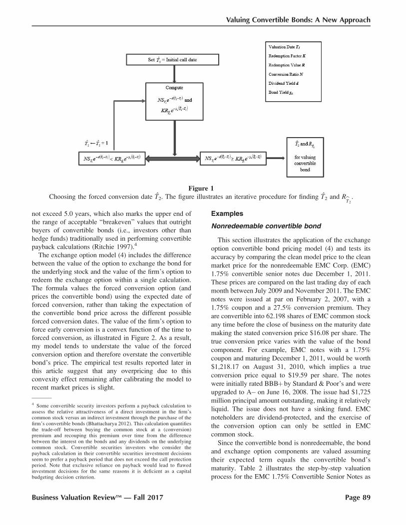
T̂2 can be found iteratively. Initially set T̂2 equal to the

earliest date the bond can be called. Calculate

NST1e�dðbT2�T1Þ. Choose as the initial optional redemption

value RbT2

and calculate KRbT2

e�ycðbT2�T1Þ. If NST1e�dðbT2�T1Þ

is greater than or equal to KRbT2

e�ycðbT2�T1Þ the initial

optional redemption date would be the assumed forced

conversion date T̂2. If NST1e�dðbT2�T1Þ is less than

KRbT2

e�ycðbT2�T1Þ, forced conversion would be unprofit-

able for the firm. Increment T̂2 by 1 and use the next

period’s optional redemption price as RbT2

. Recalculate

KRbT2

e�ycðbT2�T1Þ a n d c o m p a r e NST1e�dðbT2�T1Þ t o

KRbT2

e�ycðbT2�T1Þ. If NST1e�dðbT2�T1Þ is greater than or equal

to KRbT2

e�ycðbT2�T1Þ, the second period’s earliest optional

redemption date would be the assumed forced conver-

sion date T̂2. Otherwise, increment T̂2 by 1 again and

continue the search process. The search procedure

usually finds T̂2 after at most a few steps. Figure 1

illustrates the search procedure.

For example, suppose K¼ 1.0. Assume NST1¼ 780, d

¼ 0 , KR3e�3yc ¼ 980, KR4e�4yc ¼ 880, a n d

KR5e�5yc ¼ 780. At T̂2 ¼ 3 years, NST1, KR3e�3yc(780

, 980). At T̂2¼ 4 years, NST1,KR4e�4yc (780 , 880). At

T̂2¼ 5 years, NST1¼ KR5e�5yc (780¼ 780). Thus, the best

estimate is T̂2 – T1¼5 years. For most issues, T̂2 – T1 will



not exceed 5.0 years, which also marks the upper end of

the range of acceptable ‘‘breakeven’’ values that outright

buyers of convertible bonds (i.e., investors other than

hedge funds) traditionally used in performing convertible

payback calculations (Ritchie 1997).4

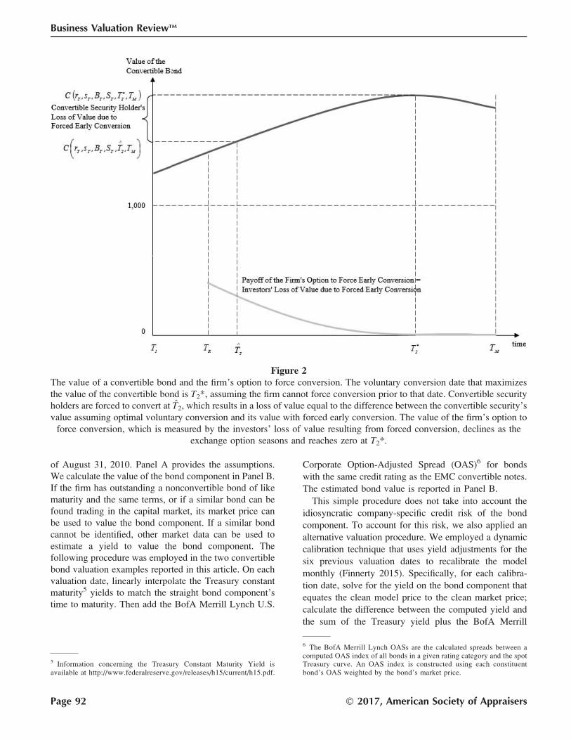
The exchange option model (4) includes the difference

between the value of the option to exchange the bond for

the underlying stock and the value of the firm’s option to

redeem the exchange option within a single calculation.

The formula values the forced conversion option (and

prices the convertible bond) using the expected date of

forced conversion, rather than taking the expectation of

the convertible bond price across the different possible

forced conversion dates. The value of the firm’s option to

force early conversion is a convex function of the time to

forced conversion, as illustrated in Figure 2. As a result,

my model tends to understate the value of the forced

conversion option and therefore overstate the convertible

bond’s price. The empirical test results reported later in

this article suggest that any overpricing due to this

convexity effect remaining after calibrating the model to

recent market prices is slight.

Examples

Nonredeemable convertible bond

This section illustrates the application of the exchange

option convertible bond pricing model (4) and tests its

accuracy by comparing the clean model price to the clean

market price for the nonredeemable EMC Corp. (EMC)

1.75% convertible senior notes due December 1, 2011.

These prices are compared on the last trading day of each

month between July 2009 and November 2011. The EMC

notes were issued at par on February 2, 2007, with a

1.75% coupon and a 27.5% conversion premium. They

are convertible into 62.198 shares of EMC common stock

any time before the close of business on the maturity date

making the stated conversion price $16.08 per share. The

true conversion price varies with the value of the bond

component. For example, EMC notes with a 1.75%

coupon and maturing December 1, 2011, would be worth

$1,218.17 on August 31, 2010, which implies a true

conversion price equal to $19.59 per share. The notes

were initially rated BBBþby Standard & Poor’s and were

upgraded to A� on June 16, 2008. The issue had $1,725

million principal amount outstanding, making it relatively

liquid. The issue does not have a sinking fund. EMC

noteholders are dividend-protected, and the exercise of

the conversion option can only be settled in EMC

common stock.

Since the convertible bond is nonredeemable, the bond

and exchange option components are valued assuming

their expected term equals the convertible bond’s

maturity. Table 2 illustrates the step-by-step valuation

process for the EMC 1.75% Convertible Senior Notes as

Figure 1Choosing the forced conversion date T̂2. The figure illustrates an iterative procedure for finding T̂2 and RbT2

.

4 Some convertible security investors perform a payback calculation toassess the relative attractiveness of a direct investment in the firm’scommon stock versus an indirect investment through the purchase of thefirm’s convertible bonds (Bhattacharya 2012). This calculation quantifiesthe trade-off between buying the common stock at a (conversion)premium and recouping this premium over time from the differencebetween the interest on the bonds and any dividends on the underlyingcommon stock. Convertible securities investors who consider thepayback calculation in their convertible securities investment decisionsseem to prefer a payback period that does not exceed the call protectionperiod. Note that exclusive reliance on payback would lead to flawedinvestment decisions for the same reasons it is deficient as a capitalbudgeting decision criterion.



Table 1Characteristics of Convertible Bonds Issued between 2003 and 2013

Investment-Grade Notes

Investment-Grade

Total

Noncallable,

Nonputable

Callable,

Nonputable

Putable,

Noncallable

Callable

and Putable

2003

No. of Issues 67 5.97% 49.25% - 44.78%

Total Face Amount ($ mil) 19,256,103,500 5.93% 3.81% - 90.26%

No. of Dividend-Protected 3 - - - 100.00%

2004

No. of Issues 94 4.26% 54.26% - 41.49%



2005

No. of Issues 51 17.65% 56.86% - 25.49%



2006

No. of Issues 65 40.00% 20.00% - 40.00%


No. of Dividend-Protected 31 35.48% - - 64.52%

2007

No. of Issues 40 55.00% 10.00% - 35.00%



2008

No. of Issues 20 40.00% 30.00% - 30.00%



2009

No. of Issues 15 93.33% - - 6.67%

Total Face Amount ($ mil) 8,565,000,000 95.97% - - 4.03%


2010

No. of Issues 7 85.71% - - 14.29%

Total Face Amount ($ mil) 4,949,403,000 90.01% - - 9.99%


2011

No. of Issues 15 80.00% - 6.67% 13.33%

Total Face Amount ($ mil) 5,307,493,000 80.14% - 10.34% 9.51%

No. of Dividend-Protected 14 78.57% - 7.14% 14.29%

2012

No. of Issues 10 100.00% - - -

Total Face Amount ($ mil) 4,360,000,000 100.00% - - -

No. of Dividend-Protected 9 100.00% - - -

2013

No. of Issues 2 100.00% - - -

Total Face Amount ($ mil) 321,602,000 100.00% - - -

No. of Dividend-Protected 1 100.00% - - -

2003-2013

No. of Issues 386 30.31% 35.23% 0.26% 34.20%

Total Face Amount ($ mil) 144,824,468,840 38.13% 2.27% 0.38% 59.22%

No. of Dividend-Protected 130 49.23% - 0.77% 50.00%

a Includes high-yield and nonrated convertible bonds.



Table 1Extended.

Non-Investment-Grade and Nonrated Notes

Total

Non-Investment-Grade

TotalaNoncallable,

Nonputable

Callable,

Nonputable

Putable,

Noncallable

Callable

and Putable

153 34.64% 26.14% - 39.22% 220

31,273,734,700 27.32% 19.29% - 53.39% 50,529,838,200

19 21.05% 10.53% - 68.42% 22

207 15.94% 14.01% 1.45% 68.60% 301

40,013,103,500 13.45% 7.82% 0.97% 77.76% 58,685,039,000

49 16.33% 4.08% 4.08% 75.51% 62

117 25.64% 16.24% 0.85% 57.26% 168

24,049,904,000 22.66% 12.68% 0.34% 64.32% 36,810,457,400

41 17.07% 9.76% - 73.17% 51

111 40.54% 14.41% 1.80% 43.24% 176

28,175,484,400 28.00% 9.02% 0.85% 62.13% 61,808,820,400

63 31.75% 11.11% 3.17% 53.97% 94

163 52.15% 5.52% 0.61% 41.72% 203

46,241,591,000 55.82% 2.32% 0.04% 41.82% 74,269,141,000

94 55.32% 3.19% - 41.49% 114

82 60.98% 12.20% 2.44% 24.39% 102

17,647,155,150 65.22% 5.12% 1.93% 27.73% 26,618,647,590

44 56.82% 4.55% - 38.64% 54

98 71.43% 10.20% 2.04% 16.33% 113

22,225,530,740 78.11% 7.53% 2.02% 12.33% 30,790,530,740

82 75.61% 8.54% 2.44% 13.41% 94

50 64.00% 10.00% 4.00% 22.00% 57

12,839,856,000 70.89% 10.82% 2.06% 16.23% 17,789,259,000

46 65.22% 8.70% 4.35% 21.74% 53

69 78.26% 4.35% 1.45% 15.94% 84

12,476,360,000 75.12% 4.12% 0.80% 19.96% 17,783,853,000

58 77.59% 5.17% 1.72% 15.52% 72

62 77.42% 4.84% - 17.74% 72

15,475,871,500 72.18% 3.53% - 24.29% 19,835,871,500

59 77.97% 5.08% - 16.95% 68

52 69.23% 17.31% 1.92% 11.54% 54

12,909,916,000 76.08% 7.94% 0.02% 15.96% 13,231,518,000

39 84.62% 5.13% - 10.26% 40

1,164 46.05% 13.14% 1.29% 39.52% 1,550

263,328,506,990 46.11% 8.31% 0.72% 44.87% 408,152,975,830

594 55.89% 6.57% 1.52% 36.03% 724



of August 31, 2010. Panel A provides the assumptions.

We calculate the value of the bond component in Panel B.

If the firm has outstanding a nonconvertible bond of like

maturity and the same terms, or if a similar bond can be

found trading in the capital market, its market price can

be used to value the bond component. If a similar bond

cannot be identified, other market data can be used to

estimate a yield to value the bond component. The

following procedure was employed in the two convertible

bond valuation examples reported in this article. On each

valuation date, linearly interpolate the Treasury constant

maturity5 yields to match the straight bond component’s

time to maturity. Then add the BofA Merrill Lynch U.S.

Corporate Option-Adjusted Spread (OAS)6 for bonds

with the same credit rating as the EMC convertible notes.

The estimated bond value is reported in Panel B.

This simple procedure does not take into account the

idiosyncratic company-specific credit risk of the bond

component. To account for this risk, we also applied an

alternative valuation procedure. We employed a dynamic

calibration technique that uses yield adjustments for the

six previous valuation dates to recalibrate the model

monthly (Finnerty 2015). Specifically, for each calibra-

tion date, solve for the yield on the bond component that

equates the clean model price to the clean market price;

calculate the difference between the computed yield and

the sum of the Treasury yield plus the BofA Merrill

Figure 2The value of a convertible bond and the firm’s option to force conversion. The voluntary conversion date that maximizes

the value of the convertible bond is T2*, assuming the firm cannot force conversion prior to that date. Convertible security

holders are forced to convert at T̂2, which results in a loss of value equal to the difference between the convertible security’s

value assuming optimal voluntary conversion and its value with forced early conversion. The value of the firm’s option to

force conversion, which is measured by the investors’ loss of value resulting from forced conversion, declines as the

exchange option seasons and reaches zero at T2*.

5 Information concerning the Treasury Constant Maturity Yield isavailable at http://www.federalreserve.gov/releases/h15/current/h15.pdf.

6 The BofA Merrill Lynch OASs are the calculated spreads between acomputed OAS index of all bonds in a given rating category and the spotTreasury curve. An OAS index is constructed using each constituentbond’s OAS weighted by the bond’s market price.



Lynch OAS; and average the six spread adjustments. Add

the average spread adjustment to the valuation date

Treasury yield plus OAS to obtain the discount rate y and

then calculate the value Bt of the straight bond

component:

Bt ¼XJ

j¼1

CFj

1þ y2

� �j ; ð6Þ

where CFj is the interest and principal payment in

semiannual period j and J is the number of periods. We

report the bond valuations obtained using this more

detailed alternative valuation procedure in Panel D of

Table 2.

Next, after valuing the bond component, value the

exchange option using equations (1)–(3). We do this in

Panel C of Table 2. Adjust the current value of the bond

component for the coupon payments expected to be paid

Table 2Illustration of the Valuation Process for the EMC Corp. Nonredeemable 1.75% Convertible Senior Notes Due

December 1, 2011

Panel A. AssumptionsValuation Date (T1) August 31, 2010 Coupon rate 1.7500%

Share Price at T1 (ST1) $18.02 Price at issue (BT1

) $1,000.00

Maturity December 1, 2011 Conversion ratio (N) 62.1980

Dividend-Protected Yes Expected conversion (T2) December 1, 2011

Continuous Dividend Yield (d) 0.0% Credit rating A�Panel B. Value of the Bond Component

Time to Expected Conversion (T2�T1) 1.25 years

Interpolated Treasury Constant Maturity Yield 0.31%

Option-Adjusted Spread (OAS), A-rated 1.77%

Bond Cash Flow Yield (c) 2.08%

Value of Straight Bond Component $995.99

Panel C. Value of the Exchange Option and the Convertible Bond1 2 3

Implied Volatility

Function

Bloomberg Six-Month

Volatility

Bloomberg Implied

Volatility

Stock Volatility (r) 35.32% 27.72% 30.45%

rz ¼ r(T2�T1)1/2 39.53% 31.03% 34.09%

RatioT1¼ NS(t)/B(t)e�cðT2�T1Þ 1.1503 1.1503 1.1503

lc ¼ ln[RatioT1] � (rz

2/2) 0.0619 0.0919 0.0819

Value of Exchange Option* $247.43 $215.22 $226.68

Value of Convertible Bond† $1,243.43 $1,211.22 $1,222.68

Reported Market Price $1,218.17 $1,218.17 $1,218.17

Pricing Error‡ 2.07% �0.57% 0.37%

Panel D. Value of the Convertible Bond under the Alternative Procedure1 2 3

Implied Volatility

Function

Bloomberg Six-Month

Volatility

Bloomberg Implied

Volatility

Average Spread Adjustment§ 3.43% �1.44% 0.49%

Bond Yield after Calibration (y) 5.50% 0.64% 2.57%

Value of Straight Bond Component $955.21 $1,013.81 $989.97


Value of Convertible Bond§ $1,231.34 $1,218.48 $1,220.18

Pricing Error‡ 1.08% 0.03% 0.16%

* Using equations (1)–(3).

† Equals value of straight bond component plus value of exchange option.

‡ Pricing error is calculated as the difference between the clean model price and the reported clean market price divided by the clean

market price.

§ For each date, solve for the yield on the bond component that equates the clean model price to the clean market price; calculate the

difference between the computed yield and the sum of the Treasury yield plus the BofA Merrill Lynch OAS; and average the spread

adjustments for the six previous valuation dates.

Business Valuation ReviewTM — Fall 2017 3


during its remaining life (the exchange option’s expected

term) to get BT1e�cðT2�T1Þ The value of the underlying

equity is NST1e�dðT2�T1Þwhen cash dividends are paid at

the rate d. The EMC noteholders are dividend-protected,

so the conversion value is unaffected by dividend

payments. Upon a dividend event, a dividend-protected

convertible bond issue automatically has the conversion

ratio adjust according to equation (5). Convertible

noteholders thus receive the value of the cash dividends

EMC will pay between the date of purchase and the date

of conversion.

The price ratio volatility equals the stock price

volatility when the convertible bond is nonredeemable.

Estimate the stock price volatility for each valuation date

by applying the implied volatility function (IVF)

methodology described in Hull and Suo (2002), which

utilizes the volatilities implied by the prices of market-

traded call and put options on a stock to express volatility

as a function of the remaining option term and money-

ness. This IVF is used to infer volatility for the stock

option being valued by extrapolating long-term volatility

from short-term exchange-traded option implied volatil-

ities. It involves fitting a skew function to the implied

volatilities. A typical skew function is of the form7

IVFðx; TÞ ¼ C0x�q þ C1logx*1ffiffiffiTp� �

þ C2 logx½ �2*1

T

� �;

ð7Þ

where x ¼ (strike/forward stock price), T ¼ time to

maturity, and C0, C2, and q are time-dependent

parameters to be estimated for each maturity and C0 is

the at-the-money volatility. The parameters are estimated

by ordinary least squares.

We also performed each valuation using two other

stock price volatility measures obtained from Bloomberg:

the six-month historical stock price volatility and the

implied stock price volatility for a three-month at-the-

money option. Both ignore the exchange option’s

moneyness but have the advantage of being readily

available on a Bloomberg screen.8 We used these

volatility estimates to test whether this simpler approach

could achieve acceptable pricing accuracy.

After valuing the exchange option, we add it to the

value of the bond component to get the model price of the

EMC convertible notes as of August 31, 2010, which we

report in Panel C of Table 2. The pricing error is between

�0.57% and 2.07% depending on the stock price

volatility estimate used. We also valued the exchange

option and the convertible bond in Panel D of Table 2 by

applying the alternative procedure that takes into account

the idiosyncratic company-specific credit risk of the bond

component. It should therefore normally provide a more

accurate valuation, but at the cost of requiring a more

complex calculation. The pricing errors, which are

reported in Panel D, are between 0.03% and 1.08% and

are uniformly lower than the pricing errors for the simple

procedure in Panel C.

We also applied the more detailed valuation procedure

at monthly intervals between July 31, 2009, and

November 30, 2011. Table 3 reports the pricing errors

for the EMC convertible notes when the exchange option

valuation model is recalibrated monthly. The median

pricing error using the IVF methodology is 0.03%, and

the mean pricing error is�0.03%. The two other volatility

estimates lead to slightly larger average pricing errors,

which are still within�1.17%.

Figure 3 illustrates how the clean model price closely

tracks the clean market price between July 31, 2009, and

November 30, 2011. It also breaks down the value of a

EMC note into its bond and exchange option component

values. Figure 4 shows how the value of the EMC

noteholders’ exchange option varies with the implied

volatility and the time to maturity as of July 31, 2009, just

after the financial crisis period ended. The exchange

option is more valuable the higher the implied volatility

and the longer the time to expiration, as option theory

predicts.

Callable convertible bond

This section compares the model price to the actual

market price for the callable (but nonputable) Maxtor

Corporation (STX) 2.375% convertible senior notes due

August 15, 2012. The STX notes were issued at par on

February 1, 2006, with a 2.375% coupon and a 23%

conversion premium. They were initially convertible into

153.1089 shares of STX common stock any time before

the close of business on the maturity date making the

stated conversion price $6.5313 per share. The conver-

sion ratio was 60.2074 shares as of the valuation date.

The true conversion price varies with the value of the

bond component. For example, STX bonds with a

2.375% coupon and maturing August 15, 2012, would

be worth $1585 on March 31, 2006, which implies a true

conversion price equal to $10.3521 per share. The notes

were initially rated BBþby Standard & Poor’s. The rating

decreased to B on December 12, 2008. The issue had

$326 million principal amount outstanding, which made

7 We obtained this skew function from the convertible bond departmentof a major broker-dealer.8 Bloomberg began reporting an implied volatility surface (IVS) forequity options July 26, 2010. Although this date falls within ourempirical testing period, we did not have a continuous series of IVSvolatilities for the entire period. Finnerty (2015) compares the pricingerrors when using IVF volatilities and Bloomberg IVS volatilities for asubsample of nonredeemable convertible bonds. He finds no statisticallysignificant difference in pricing errors between the valuations based onthe IVF and IVS volatilities.



Figure 3Components of the value of the nonredeemable EMC Corp. 1.75% convertible senior notes due December 1, 2011. This

figure plots the clean market price and the clean model price and plots the value of the straight bond component and the

value of the exchange option at monthly intervals between July 2009 and November 2011.

Table 3Pricing Errors for the EMC Corp. Nonredeemable 1.75% Convertible Senior Notes Due December 1, 2011*

Implied Volatility Function Bloomberg Six-Month Volatility Bloomberg Implied Volatility

Number of Observations 28 28 28

Maximum Difference (%) 2.30 1.28 3.18

Minimum Difference (%) �2.21 �4.11 �3.28

Mean Difference (%) �0.03 �1.17 �0.75

Mean Absolute Difference (%) 0.58 1.30 1.14

Median Difference (%) 0.03 �0.80 �0.81

Median Absolute Difference (%) 0.42 0.92 0.85

Standard Deviation (%) 0.84 1.34 1.27

Note. This table uses the exchange option convertible bond pricing model to value the nonredeemable EMC Corp. 1.75% convertible

senior notes due December 1, 2011, between July 2009 and November 2011. The model price before calibration is estimated assuming

that the bond component of the convertible note has a yield consistent with the Treasury constant maturity yield term structure plus the

BofA Merrill Lynch U.S. corporate OAS for bonds with commensurate credit rating on each valuation date. The calibration technique

uses a moving estimation window with yields for the preceding six months as the calibration period. Three methodologies are used to

calculate the volatility of the exchange option: (1) Implied Volatility Function; (2) Bloomberg six-month historical stock price volatility;

and (3) Bloomberg three-month at-the-money implied volatility.

* Pricing error is calculated as the difference between the clean model price and the reported clean market price divided by the clean

market price.



it relatively liquid. The issue does not have a sinking

fund. STX noteholders are dividend-protected, and the

exercise of the conversion option can be settled only in

STX common stock.

The STX notes were redeemable beginning on August

20, 2010, at a price equal to 100.68% of the principal

amount plus accrued and unpaid interest to, but not

including, the redemption date. If STX decides to redeem

part or all of the notes, it would have to give the holders at

least 30 days’ but no more than 60 days’ notice. STX

would pay the conversion value unless it fell below the

redemption value. The STX convertible notes are valued

assuming zero redemption cushion, K ¼ 1, and R ¼$1006.80.

We use the stopping time methodology to determine

the notes’ expected forced conversion date T̂2 and

equation (4) to value the notes. Table 4 illustrates the

step-by-step valuation process for the STX 2.375%

convertible senior notes as of March 31, 2010. The

earliest call date is August 20, 2010. Investors expected

STX to force conversion soon after the first call date

(around October 4, 2010). The present value of the

effective redemption price, if forced conversion is

expected in 0.51 years, is $971.88 per bond, which is

less than the dividend-adjusted price of the underlying

STX common stock (d¼ 0), $971.90 per bond. Set T̂2�T1

¼0.51 and RbT2

¼$1006.80 since the STX exchange option

was expected to be in-the-money. Panel A provides the

other assumptions. The value of the straight bond

component using the basic procedure is $902.33, which

is calculated in Panel B. The value of the exchange option

and the value of the convertible bond are calculated in

Panel C using three stock volatility measures. The pricing

errors are between �4.58% and �5.09% and average a

little under 5% underpricing.

Panel D of Table 4 values the STX 2.375% convertible

senior notes using the more detailed alternative proce-

dure, which takes into account the idiosyncratic compa-

ny-specific credit risk of the bond component more

accurately by recalibrating the model monthly. As

Figure 4Value of bondholders’ exchange option as a function of the implied volatility and the time to expiration of the option. The

nonredeemable EMC Corp. 1.75% convertible senior notes due December 1, 2011, are valued and the sensitivities are

calculated as of July 31, 2009.



expected, the more detailed procedure achieves greater

accuracy with pricing errors between �2.16% and

�3.43% and averaging less than 3% underpricing.

Table 5 reports the pricing errors for the STX 2.375%

convertible senior notes when they are valued on the last

trading day of each month between July 2009 and August

2010 and the model is recalibrated monthly. The median

pricing error using the IVF methodology is�0.84%, and

the mean pricing error is�1.22%. The two other volatility

estimates lead to somewhat larger average pricing errors.

Figure 5 compares the clean market price to the clean

model price for the STX convertible notes under two

assumptions: the firm forces conversion optimally and the

firm never forces conversion. The model price assuming

optimal forced conversion closely tracks the market price,

but the model price assuming there will be no forced

Table 4Illustration of the Valuation Process for the Maxtor Corp. Callable 2.375% Convertible Senior Notes Due August 15,

2012

Panel A. AssumptionsValuation Date (T1) March 31, 2010 Coupon rate 2.3750%

Share Price at T1 (ST1) $16.14 Price at issue (BT1

) $1,000.00

Maturity August 15, 2012 Conversion ratio (N) 60.2074

Dividend-Protected Yes Expected conversion (T2) October 4, 2010

Continuous Dividend Yield (d) 0.0% Credit rating B

Panel B. Value of the Bond ComponentTime to Expected Conversion (T2 � T1) 0.51 years

Interpolated Treasury Constant Maturity Yield 1.24%

Option-Adjusted Spread (OAS), B-rated 5.67%

Bond Cash Flow Yield (c) 6.91%

Value of Straight Bond Component $902.33

Panel C. Value of the Exchange Option and the Convertible Bond1 2 3

Implied Volatility

Function

Bloomberg Six-Month

Volatility

Bloomberg Implied

Volatility

Stock Volatility (r) 48.01% 45.75% 47.82%

rz ¼ r(T2�T1)1/2 34.32% 32.71% 34.18%

RatioT1¼ NS(t)/B(t)e�cðT2�T1Þ 1.0902 1.0902 1.0902

lc ¼ ln[RatioT1]�(rz

2/2) 0.0274 0.0328 0.0279



Reported Market Price $1,125.00 $1,125.00 $1,125.00

Pricing Error‡ �4.58% �5.09% �4.63%

Panel D. Value of the Convertible Bond under the Alternative Procedure1 2 3

Implied Volatility

Function

Bloomberg Six-Month

Volatility

Bloomberg Implied

Volatility

Average Spread Adjustment§ �1.55% �1.84% �2.61%

Bond Yield after Calibration (y) 5.36% 5.07% 4.30%

Value of Straight Bond Component $934.29 $940.51 $957.03



Pricing Error‡ �3.18% �3.43% �2.16%

* Using equations (1)–(3).

† Equals value of straight bond component plus value of exchange option.

‡ Pricing error is calculated as the difference between the clean model price and the reported clean market price divided by the clean

market price.

§ For each date, solve for the yield on the bond component that equates the clean model price to the clean market price; calculate the

difference between the computed yield and the sum of the Treasury yield plus the BofA Merrill Lynch OAS; and average the spread

adjustments for the six previous valuation dates.



Table 5Pricing Errors for the Maxtor Corp. Callable 2.375% Convertible Senior Notes Due August 15, 2012*

Implied Volatility Function Bloomberg Six-Month Volatility Bloomberg Implied Volatility

Number of Observations 13 13 13

Maximum Difference (%) 9.22 12.89 12.74

Minimum Difference (%) �11.46 �15.39 �12.03

Mean Difference (%) �1.22 �3.54 �1.68

Mean Absolute Difference (%) 3.94 6.91 5.47

Median Difference (%) �0.84 �3.42 �2.16

Median Absolute Difference (%) 3.18 7.71 4.83

Standard Deviation (%) 5.22 7.63 6.71

Note. This table uses the exchange option convertible bond pricing model to value the callable Maxtor Corp. 2.375% convertible senior

notes due August 15, 2012, between July 2009 and August 2010. (TRACE stopped providing market price data for this bond after

August 2010.)

The model price before calibration is estimated assuming that the bond component of the convertible note has a yield consistent with the

Treasury constant maturity yield term structure plus the BofA Merrill Lynch U.S. corporate OAS for bonds with commensurate credit

rating on each valuation date. The calibration technique uses a moving estimation window with yields for the preceding six months as

the calibration period. Three methodologies are used to calculate the volatility of the exchange option: (1) Implied Volatility Function,

(2) Bloomberg six-month historical stock price volatility, and (3) Bloomberg three-month at-the-money implied volatility.

* Pricing error is calculated as the difference between the clean model price and the reported clean market price divided by the clean

market price.

Figure 5Model price versus market price of the callable and nonputable Maxtor Corp. 2.375% convertible senior notes due August

15, 2012. The figure plots the clean model price and the clean market price at monthly intervals between July 2009 and

August 2010. The expected time to forced conversion is determined using the stopping time model. The figure also plots

the clean model price of the convertible note assuming no forced conversion.



conversion significantly overstates the market price for

almost the entire period, which confirms that forced

conversion risk is priced by the market.

Finnerty (2015) describes how the valuation model (4)

can be further extended to value convertible bonds that

are both callable and putable.

Empirical Tests

Finnerty (2015) tested the accuracy of the exchange

option convertible bond pricing model (4) using market

prices for a sample of 148 convertible bond issues.

Month-end TRACE bond prices were obtained from

Bloomberg for the period January 31, 2006, through

January 31, 2014.9 Clean model prices were compared to

observed clean market prices monthly for three subsam-

ples of bonds issued between January 2, 2006, and

December 31, 2010, with a principal amount of at least

$100 million: eighty-seven nonredeemable (noncallable

and nonputable), six callable (but nonputable), and fifty-

five callable and putable convertible bonds.

The model’s accuracy was tested based on month-end

prices between January 2006 and January 2014. Since

this period includes the financial crisis of 2008–2009, the

testing was performed for the full period and for three

subperiods: precrisis (January 2006 through December

2007), crisis period (January 2008 through June 2009),

and postcrisis (July 2009 through January 2014). The

model’s pricing accuracy was also investigated during the

short selling ban period (September 2008 through

February 2009). The short selling restrictions, including

the outright ban on short selling the SEC imposed

between September 19, 2008, and October 8, 2008,

severely disrupted the convertibles market. The SEC’s

short selling restrictions prohibited the short selling that

hedge funds use to hedge their convertible bond

investments making convertible bond investing riskier

and driving some hedge funds from the market. As a

result, the model would be expected to overprice

convertible securities during the short sale ban period.

To value each convertible bond, Finnerty (2015)

valued the straight bond component using the more

detailed valuation procedure described earlier in the

article, applied equations (1)–(3) to value the exchange

option, and summed the two component values. So long

as the convertible is dividend-protected, a zero redemp-

tion cushion was assumed. Finnerty (2015) also assumed

optimal option exercise by firms and investors. Common

stock volatility was used in place of the price ratio

volatility in equations (1)–(4). Stock price volatility was

estimated for each valuation date by applying the IVF

methodology described in Hull and Suo (2002), which

utilizes the volatilities implied by the prices of market-

traded call and put options on a stock to express volatility

as a function of the remaining option term and money-

ness. Each convertible issue was also valued using two

other stock price volatility measures that were obtained

from Bloomberg: the six-month historical stock price

volatility and the implied stock price volatility for a three-

month at-the-money option. Using these volatility

estimates tests whether this simpler approach could

achieve acceptable pricing accuracy.

Table 6 reports the median and mean pricing errors for

the nonredeemable convertible bond subsample in Panel

A, the callable convertible bond subsample in Panel B,

and the callable and putable convertible bond subsample

in Panel C. The simple arithmetic average for each

statistic is reported. The clean model price is calculated

for each convertible outstanding at each month-end. The

pricing error is the difference between the clean model

price and the clean market price divided by the clean

market price.

For the full period and IVF volatility, the average

median (mean) pricing errors are�0.04% (0.22%) for the

nonredeemable convertible bonds; �0.50% (�0.16%) for

callable convertible bonds; �0.38% (0.24%) for callable

and putable convertible bonds; and �0.18% (0.21%)

overall. The Bloomberg six-month and at-the-money

implied volatilities lead to similar average pricing errors.

All the average median and mean pricing errors are within

60.63% during the full period, although they are

somewhat smaller for the nonredeemable convertibles

than for the redeemable convertibles.

The average median and average mean pricing errors

for the nonredeemable convertible bonds are smallest

during the postcrisis period and largest during the short

selling ban period for all three volatility estimation

methods. They are also largest during the short selling

ban period for all three volatility estimation methods for

callable convertibles and callable and putable convert-

ibles. No clear pattern of dominance is evident in the

precrisis, crisis, and postcrisis subperiod pricing errors for

callable convertibles or callable and putable convertibles.

No clear pattern of dominance is evident in the full period

average pricing errors across the three volatility estima-

tion methods and the three samples of convertibles.

9 The sample of convertible bonds has the following characteristics: (a)issued in the United States between January 2, 2006, and December 31,2010; (b) initial issue size of $100 million or greater; (c) convertible intothe bond issuer’s common stock; (d) TRACE prices available at leastweekly between the issue date and the earliest of conversion,redemption, or January 31, 2014; (e) rated by Moody’s InvestorsService or Standard & Poor’s throughout the sample period; and (f) fixedcoupon rate. The sample end date was chosen so as to have at least threeyears of pricing data for each bond to test the model. Characteristics (b)and (d) are designed to exclude relatively illiquid issues; (c) excludesbonds exchangeable either for another firm’s common stock or for abasket of stocks; (e) is needed to value the straight bond component; and(f) is designed to exclude bonds with contingent or floating interest rates.



Tab

le6

Tes

tsof

the

Exch

ange

Opti

on

Conver

tible

Bond

Pri

cing

Model

’sA

ver

age

Pri

cing

Err

ors

Imp

lied

Vo

lati

lity

Fu

nct

ion

Blo

om

ber

gS

ix-M

on

thV

ola

tili

tyB

loo

mb

erg

Imp

lied

Vo

lati

lity

Fu

llP

re-

Du

rin

gP

ost

-B

anF

ull

Pre

-D

uri

ng

Po

st-

Ban

Fu

llP

re-

Du

rin

gP

ost

-B

an

Pa

nel

A.

No

nre

dee

ma

ble

Co

nv

erti

ble

Bo

nd

sA

vg

.N

o.

of

Ob

serv

atio

ns

per

Bo

nd

52

71

33

25

54

71

53

25

53

71

53

25

To

tal

Nu

mb

ero

fO

bse

rvat

ion

s4

55

46

20

11

42

27

92

40

84

66

25

95

12

74

27

93

46

74

60

55

91

12

64

27

51

46

0

Av

g.

Min

.D

iffe

ren

ce(%

)(8

.15

)(1

.67

)(9

.99

)(5

.59

)(6

.39

)(1

0.6

8)

(2.4

5)

(10

.22

)(8

.81

)(3

.47

)(9

.77

)(2

.03

)(1

2.2

8)

(7.0

9)

(7.3

4)

Av

g.

25

thP

erce

nti

le(%

)(0

.65

)0

.05

(0.8

7)

(0.4

4)

(0.3

2)

(0.9

2)

0.0

7(0

.74

)(0

.75

)0

.39

(0.8

3)

0.0

0(1

.11

)(0

.57

)(0

.18

)

Av

g.

Med

ian

Dif

fere

nce

(%)

(0.0

4)

1.3

7(0

.61

)(0

.25

)2

.14

(0.4

8)

2.5

51

.29

(0.5

4)

7.7

5(0

.37

)1

.15

(1.0

3)

(0.2

8)

5.0

6

Av

g.

75

thP

erce

nti

le(%

)0

.86

3.7

2(0

.25

)0

.21

5.7

00

.06

6.4

34

.13

(0.3

9)

18

.30

0.2

93

.21

(0.9

3)

0.2

11

2.4

1

Av

g.

Max

.D

iffe

ren

ce(%

)1

1.3

04

.19

15

.61

5.8

61

2.4

61

6.3

57

.41

21

.57

7.2

41

9.4

11

6.2

13

.68

22

.99

7.7

42

0.9

7

Av

g.

Mea

nD

iffe

ren

ce(%

)0

.22

1.2

30

.45

(0.1

8)

2.5

8(0

.11

)2

.57

2.9

5(0

.77

)7

.83

(0.0

1)

1.0

21

.07

(0.2

4)

5.9

1

Pa

nel

B.

Ca

lla

ble

(bu

tN

on

-Pu

tab

le)

Co

nv

erti

ble

Bo

nd

sA

vg

.N

o.

of

Ob

serv

atio

ns

per

Bo

nd

52

18

16

18

46

22

61

71

86

57

21

17

18

6

To

tal

No

.o

fO

bse

rvat

ion

s3

12

10

89

41

10

26

37

21

58

10

41

10

34

34

21

28

10

41

10

34

Av

g.

Min

.D

iffe

ren

ce(%

)(8

.10

)(7

.49

)(1

1.1

2)

(9.5

6)

(2.4

8)

(9.4

8)

(7.1

0)

(7.0

0)

(11

.22

)(4

.70

)(9

.11

)(9

.26

)(1

2.9

3)

(9.4

0)

(5.1

0)

Av

g.

25

thP

erce

nti

le(%

)(3

.02

)(3

.04

)(3

.00

)(3

.23

)(1

.02

)(2

.54

)(2

.78

)(1

.72

)(4

.08

)(1

.94

)(3

.12

)(3

.39

)(2

.30

)(3

.23

)(2

.58

)

Av

g.

Med

ian

Dif

fere

nce

(%)

(0.5

0)

(0.5

6)

(0.3

5)

(0.8

2)

2.9

00

.44

(0.1

0)

1.8

2(2

.30

)1

.33

(0.6

3)

(1.1

2)

1.0

1(0

.83

)0

.18

Av

g.

75

thP

erce

nti

le(%

)2

.88

2.4

93

.27

2.4

08

.12

4.3

23

.24

6.4

80

.24

5.5

82

.95

1.8

95

.45

2.4

64

.17

Av

g.

Max

.D

iffe

ren

ce(%

)1

1.9

68

.16

13

.97

11

.97

13

.32

12

.32

8.9

81

3.1

61

2.8

81

1.2

31

5.2

41

1.2

51

5.5

31

2.8

51

5.2

7

Av

g.

Mea

nD

iffe

ren

ce(%

)(0

.16

)(0

.30

)0

.32

(0.7

0)

4.8

00

.44

0.1

62

.47

(1.9

7)

2.9

8(0

.31

)(0

.59

)0

.85

(1.1

1)

3.2

8

Pa

nel

C.

Ca

lla

ble

an

dP

uta

ble

Co

nv

erti

ble

Bo

nd

sA

vg

.N

o.

of

Ob

serv

atio

ns

per

Bo

nd

49

51

43

05

50

61

43

05

49

51

43

05

To

tal

No

.o

fO

bse

rvat

ion

s2

68

62

84

74

31

65

92

57

27

74

32

37

87

16

64

28

02

70

82

86

75

41

66

82

63

Av

g.

Min

.D

iffe

ren

ce(%

)(1

5.3

6)

(1.3

1)

(15

.41

)(1

0.4

2)

(6.2

0)

(15

.10

)(2

.72

)(1

2.5

9)

(12

.40

)(4

.00

)(1

4.4

3)

(1.3

6)

(13

.79

)(1

0.3

3)

(5.9

8)

Av

g.

25

thP

erce

nti

le(%

)(2

.82

)(0

.84

)(5

.47

)(2

.74

)(0

.44

)(3

.15

)(1

.36

)(2

.50

)(3

.65

)0

.44

(2.5

7)

(0.6

2)

(4.4

9)

(2.5

7)

(1.2

0)

Av

g.

Med

ian

Dif

fere

nce

(%)

(0.3

8)

0.6

4(0

.15

)(0

.58

)7

.87

(0.3

1)

0.8

40

.95

(0.9

4)

8.7

7(0

.27

)0

.64

0.0

2(0

.60

)7

.34

Av

g.

75

thP

erce

nti

le(%

)2

.36

3.0

05

.60

1.4

81

7.7

52

.89

3.2

06

.81

1.4

11

8.6

62

.16

2.7

85

.18

1.5

01

5.4

1

Av

g.

Max

.D

iffe

ren

ce(%

)2

6.9

05

.79

26

.26

10

.23

27

.06

26

.57

6.4

22

7.9

78

.36

27

.49

24

.99

5.8

52

4.0

49

.35

24

.88

Av

g.

Mea

nD

iffe

ren

ce(%

)0

.24

1.4

41

.38

(0.4

8)

9.2

90

.36

1.1

43

.30

(1.1

8)

11

.34

0.2

41

.50

1.4

1(0

.50

)8

.30

No

te.

Th

ista

ble

rep

ort

sth

em

ean

and

med

ian

per

cen

tag

ep

rici

ng

erro

rsfo

rth

eex

chan

ge

op

tio

nco

nv

erti

ble

bo

nd

val

uat

ion

mo

del

for

87

no

nre

dee

mab

leco

nv

erti

ble

bo

nd

sin

Pan

elA

,si

xca

llab

le(b

ut

no

tp

uta

ble

)co

nv

erti

ble

bo

nd

sin

Pan

elB

,an

dfi

fty

-fiv

eca

llab

lean

dp

uta

ble

con

ver

tible

bo

nd

sin

Pan

elC

,in

each

case

acro

ssth

efu

llsa

mp

lep

erio

das

wel

las

fou

rsu

bp

erio

ds.

Fu

lld

eno

tes

the

full

sam

ple

per

iod

,w

hic

hex

ten

ds

fro

mth

eis

sue

dat

eto

the

earl

ier

of

the

bo

nd

’sm

atu

rity

and

Jan

uar

y3

1,

20

14

.P

re-

den

ote

sth

e

pre

cris

isp

erio

den

din

go

nD

ecem

ber

31

,2

00

7;

Du

rin

gd

eno

tes

the

fin

anci

alcr

isis

per

iod

,w

hic

hex

ten

ds

fro

mJa

nu

ary

2,

20

08

,th

rou

gh

Jun

e3

0,

20

09

;P

ost

-d

eno

tes

the

po

stcr

isis

per

iod

,w

hic

hb

egin

sJu

ly1

,2

00

9;

and

Ban

den

ote

sth

esh

ort

sell

ing

ban

per

iod

,w

hic

hex

ten

ds

fro

mS

epte

mb

er1

,2

00

8,to

Feb

ruar

y2

8,2

00

9.P

erce

nta

ge

pri

cin

ger

ror

isca

lcu

late

das

the

dif

fere

nce

bet

wee

nth

ecl

ean

mo

del

pri

cean

dth

ecl

ean

mar

ket

pri

ced

ivid

edb

yth

ecl

ean

mar

ket

pri

ce.T

hre

em

eth

od

olo

gie

sar

eu

sed

toca

lcu

late

the

vo

lati

lity

of

the

exch

ang

eo

pti

on

:(1

)Im

pli

edV

ola

tili

tyF

un

ctio

n,

(2)

Blo

om

ber

gsi

x-m

on

thh

isto

rica

lst

ock

pri

cev

ola

tili

ty,

and

(3)

Blo

om

ber

gth

ree-

mo

nth

at-t

he-

mo

ney

imp

lied

vo

lati

lity

.T

he

firs

tro

wo

fea

chp

anel

rep

ort

sth

eav

erag

en

um

ber

of

ob

serv

atio

ns

per

bo

nd

(ro

un

ded

)ac

ross

all

the

mo

nth

sfo

rw

hic

hth

ere

are

avai

lab

lem

ark

etp

rice

s.T

he

tota

l

nu

mb

ero

fm

on

thly

ob

serv

atio

ns

iseq

ual

toth

eav

erag

en

um

ber

of

ob

serv

atio

ns

per

bo

nd

mu

ltip

lied

by

the

sam

ple

size

.S

ixst

atis

tics

are

calc

ula

ted

for

the

seri

eso

fm

on

thly

pri

ces

for

each

bo

nd

:th

em

inim

um

,2

5th

per

cen

tile

,m

edia

n,

75

thp

erce

nti

le,

max

imu

m,

and

mea

no

fth

em

on

thly

per

cen

tag

eer

rors

.T

he

tab

lere

po

rts

the

aver

age

val

ue

for

each

stat

isti

cfo

rth

eei

gh

ty-s

even

no

nre

dee

mab

leb

on

ds,

the

six

call

able

bo

nd

s,an

dth

efi

fty

-fiv

eca

llab

lean

dp

uta

ble

bo

nd

sfo

rth

efu

llte

stp

erio

dan

dfo

rea

chsu

bp

erio

dan

dfo

rea

ch

of

the

thre

ev

ola

tili

tym

eth

od

olo

gie

s.N

um

ber

wit

hin

par

enth

eses

ind

icat

esa

neg

ativ

ev

alu

e.



Two conclusions emerge from this analysis. The model

is more accurate in valuing nonredeemable and callable

(but not putable) convertibles than in valuing callable and

putable convertibles. Second, although the IVF estimate

generally results in more accurate valuations, using the

readily available Bloomberg implied volatility in place of

the IVF estimate results in little loss of accuracy.

Conclusion

This article describes a new closed-form contingent-

claims model for valuing a convertible bond. The model

values convertibles as the sum of the value of the straight

bond component and the value of the option to exchange

the straight bond for the underlying conversion shares.

The article provides explicit formulas for the value of the

exchange option and the value of the convertible bond. It

also compares market and model prices for a sample of

148 convertible bonds. The average median and mean

pricing errors are�0.18% and 0.21%, respectively, which

are within the average bid-ask spread for convertibles

during the postcrisis period.

The closed-form exchange option pricing model is easy

to use. Calculate the value of the straight bond and add

the value of the exchange option. The model can be

extended to value putable convertibles. Moreover, there is

little loss of pricing accuracy when the firm’s stock price

volatility is used in place of the price ratio volatility. This

finding is consistent with the general valuation practice of

assuming that the interest rate is constant and the firm’s

share price is the only source of volatility.

References

Ammann, Manuel, Axel Kind, and Christian Wilde.

2003. ‘‘Are Convertible Bonds Underpriced? An

Analysis of the French Market.’’ Journal of Banking

& Finance 27 (April):635–653.

Asquith, Paul. 1995. ‘‘Convertible Bonds Are Not Called

Late.’’ Journal of Finance 50 (September):1275–1289.

Asquith, Paul, and David W. Mullins, Jr. 1991.

‘‘Convertible Debt: Corporate Call Policy and Volun-

tary Conversion.’’ Journal of Finance 46 (Septem-

ber):1273–1290.

Bhattacharya, Mihir. 2012. ‘‘Convertible Securities: Their

Structures, Valuation, and Trading.’’ In The Handbook

of Fixed Income Securities. 8th ed. Ed. Frank J.

Fabozzi. New York: McGraw-Hill.

Black, Fischer, and Myron Scholes. 1973. ‘‘The Pricing

of Options and Corporate Liabilities.’’ Journal of

Political Economy 81 (May-June):637–659.

Brennan, Michael J., and Eduardo S. Schwartz. 1977.

‘‘Convertible Bonds: Valuation and Optimal Strategies

for Call and Conversion.’’ Journal of Finance 32

(December):1699–1715.


‘‘Analyzing Convertible Bonds.’’ Journal of Financial

and Quantitative Analysis 15 (November):907–929.


‘‘The Case for Convertibles.’’ Journal of Applied

Corporate Finance 1 (Summer):55–64.

Brown, Stephen J., Bruce D. Grundy, Craig M. Lewis,

and Patrick Verwijmeren. 2012. ‘‘Convertibles and

Hedge Funds as Distributors of Equity Exposure.’’

Review of Financial Studies 25 (October):3077–3112.

Carayannopoulos, Peter, and Madhu Kalimipalli. 2003.

‘‘Convertible Bond Prices and Inherent Biases.’’

Journal of Fixed Income 13 (December):64–73.

EMC Corporation. 2007. Prospectus for 1.75% Convert-

ible Senior Notes due December 1, 2011. February 2.

Finnerty, John D. 2015. ‘‘Valuing Convertible Bonds and

the Option to Exchange Bonds for Stock.’’ Journal of

Corporate Finance 31 (April):91–115.

Green, Richard. 1984. ‘‘Investment Incentives, Debt, and

Warrants.’’ Journal of Financial Economics 13

(March):115–136.

Grundy, Bruce D., and Patrick Verwijmeren. 2012.

‘‘Dividend-Protected Convertible Bonds and the Dis-

appearance of Call Delay.’’ University of Melbourne

working paper, June 23.

Hillion, Pierre, and Theo Vermaelen. 2004. ‘‘Death Spiral

Convertibles.’’ Journal of Financial Economics 71

(February):381–415.

Horne, Jonathan L., and Chris P. Dialynas. 2012.

‘‘Convertible Securities and Their Investment Applica-

tion.’’ In The Handbook of Fixed Income Securities. 8th

ed. Ed. Frank J. Fabozzi. New York: McGraw-Hill.

Hull, John C. 2012. Options, Futures, and Other

Derivatives. 8th ed. Upper Saddle River, NJ: Prentice

Hall.

Hull, John, and Wulin Suo. 2002. ‘‘A Methodology for

Assessing Model Risk and Its Application to the

Implied Volatility Function Model.’’ Journal of

Financial and Quantitative Analysis 37 (June):297–

318.

Hung, Mao-Wei, and Jr-Yan Wang. 2002. ‘‘Pricing

Convertible Bonds Subject to Default Risk.’’ Journal

of Derivatives 10 (Winter):75–87.

Ingersoll, Jonathan E., Jr. 1977. ‘‘A Contingent-Claims

Valuation of Convertible Securities.’’ Journal of

Financial Economics 4 (May):289–321.

Jarrow, Robert A., and Stuart M. Turnbull. 1995. ‘‘The

Pricing and Hedging of Options on Financial Securities



Subject to Credit Risk.’’ Journal of Finance 50

(March):53–85.

Kobayashi, Takao, Naruhisa Nakagawa, and Akihiko

Takahashi. 2001. ‘‘Pricing Convertible Bonds with

Default Risk.’’ Journal of Fixed Income 11 (Decem-

ber):20–29.

Lewis, Craig M., Richard J. Rogalski, and James K.

Seward. 1998. ‘‘Agency Problems, Information Asym-

metries, and Convertible Debt Security Design.’’

Journal of Financial Intermediation 7 (January):32–59.

Lewis, Craig M., and Patrick Verwijmeren. 2011.

‘‘Convertible Security Design and Contract Innova-

tion.’’ Journal of Corporate Finance 17 (Septem-

ber):809–831.

Margrabe, William. 1978. ‘‘The Value of an Option to

Exchange One Asset for Another.’’ Journal of Finance

33 (March):177–186.

Maxtor Corporation. 2006. Prospectus for 2.375%

Convertible Senior Notes due August 15, 2012.

February 1.

Mayers, David. 1988. ‘‘Why Firms Issue Convertible

Bonds: The Matching of Financial and Real Investment

Options.’’ Journal of Financial Economics 47 (Janu-

ary):83–102.

McConnell, John J., and Eduardo S. Schwartz. 1986.

‘‘LYON Taming.’’ Journal of Finance 41 (July):561–

576.

Merton, Robert C. 1973. ‘‘Theory of Rational Option

Pricing.’’ Bell Journal of Economics and ManagementScience 4 (Spring):141–183.

Merton, Robert C. 1974. ‘‘On the Pricing of Corporate

Debt: The Risk Structure of Interest Rates.’’ Journal ofFinance 29 (May):449–470.

Nyborg, Kjell G. 1995. ‘‘Convertible Debt as Delayed

Equity: Forced versus Voluntary Conversion and the

Information Role of Call Policy.’’ Journal of FinancialIntermediation 4 (October):358–395.

Nyborg, Kjell G. 1996. ‘‘The Use and Pricing of

Convertible Bonds.’’ Applied Mathematical Finance 3

(September):167–190.

Ritchie, John C., Jr. 1997. ‘‘Convertible Securities.’’ In

The Handbook of Fixed Income Securities. 5th ed. Ed.

Frank J. Fabozzi. Chicago: Irwin.

Stein, Jeremy C. 1992. ‘‘Convertible Bonds as Backdoor

Equity Financing.’’ Journal of Financial Economics 32

(August):3–22.

Tsiveriotis, Kostas, and Chris Fernandes. 1998. ‘‘Valuing

Convertible Bonds with Credit Risk.’’ Journal of FixedIncome 8 (September):95–102.



valuing convertible bonds: a new approach · 2018-12-27 · requires a contingent claims valuation...

Documents