1

Valuing Derivatives: Funding Value Adjustments and Fair Value*

John Hull and Alan White

Joseph L. Rotman School of Management

University of Toronto

April 2013

ABSTRACT

Derivatives models are used by dealers for two purposes. They are used to calculate the fair

value of the derivatives book for accounting purposes and they are used by traders to choose

trades that improve the profitability of the derivatives group, as measured by senior management.

Given the way that the performance of the derivatives group is typically measured, it is not

possible to develop a single model that serves both purposes. Traders want to incorporate a

funding value adjustment (FVA) in valuations to reflect the funding costs they are charged, but

this can lead to prices that are different from fair value. This paper concludes that, if an FVA is

made, the best practice is to use two models, one for determining breakeven trading prices, the

other for hedging and marking to market.

*A very preliminary version of this paper was titled “Should a Derivatives Dealer make a

Funding Value Adjustment?”

2

Valuing Derivatives: Funding Value Adjustments and Fair Value

One of the most controversial issues for a derivatives dealer in the last few years has been

whether or not to make what is known as a “funding value adjustment” (FVA). This is an

adjustment to the value of a derivative or a derivatives portfolio designed to reflect the dealer’s

average funding costs. Theoretical arguments indicate that the adjustment should not be made.

But, in practice, many dealers find these theoretical arguments unconvincing and choose to make

the adjustment anyway.1 This paper examines the issues raised by FVA. It is more

comprehensive and has a more managerial focus than Hull and White (2012b)

The theoretical valuation of a derivative nearly always involves an application of risk neutral

valuation. In this, expected cash flows are estimated in a risk-neutral world and discounted using

a “risk-free” interest rate. The interest rate serves two purposes. It is used as the discount rate

and it enables risk-neutral growth rates to be calculated. The economic rationale for using the

risk-free rate is the riskless hedging argument presented in Black and Scholes (1973) and Merton

(1973). This argument is reproduced in the appendix with general assumptions about the funding

rate for a) the derivative and b) the instrument used to hedge the derivative.2 It is sometimes

assumed that risk-neutral valuation can be used only when delta hedging of the underlying risk is

possible.3 This is not so. Equilibrium arguments similar to those in the original Black and

Scholes paper show that the Black-Scholes-Merton differential equation, and therefore risk-

neutral valuation, applies whether or not hedging is possible. Indeed, many applications of

derivatives pricing (for example, the real options approach to capital budgeting) are based on risk

neutral valuation when the underlying risks cannot be hedged.

Prior to the credit crisis that started in 2007, dealers used interest rates calculated from LIBOR

and LIBOR-swap rates to value derivatives. Post-crisis, most dealers have used overnight-

indexed swap (OIS) rates to determine the applicable interest rates for fully collateralized

1 See for example Ernst and Young (2012).

2 See also Piterbarg (2010) for this type of extension of Black-Scholes-Merton.

3 See for example Burgard and Kjaer (2011)

3

transactions.4 This means that in practice OIS rates are used for most interdealer transactions

because these transactions are almost invariably fully collateralized.

It is tempting to say that the interest rates used in the valuation of derivatives reflects the dealers’

best estimate of the risk-free rate. In fact, this has never been the case. The “risk-free” rates used

in derivatives valuation have always reflected funding costs. As mentioned earlier, prior to the

crisis LIBOR and LIBOR-swap rates were used as “risk-free” rates. The reason was that LIBOR

was a good approximation to the dealers’ short-term funding costs and LIBOR-swap rates are the

longer-term rates corresponding to continually refreshed LIBOR rates.5 The current use of OIS

discounting for fully collateralized transactions is based on the argument that fully collateralized

transactions are funded by collateral. If this collateral is cash, the interest rate paid is usually the

overnight federal funds rate and the OIS rate is a longer-term rate corresponding to a continually

refreshed overnight federal funds rate.6

Consistent with their view that the rates used to value derivatives should reflect funding costs,

derivatives dealers are advancing the argument that they should incorporate their funding costs

into the valuation of non-collateralized transactions. This leads to what is referred to as a

“funding value adjustment” (FVA).7 The purpose of FVA is to move valuations from those given

by the valuation models in a dealer’s systems to those that incorporate the dealer’s average

funding costs. The precise definition of FVA therefore depends on a) the model in the dealer’s

systems and b) the model that incorporates funding costs. FVA is the difference between the

valuations given by these two models.

4 See Hull and White (2012a) for a discussion of OIS rates.

5 See Collin Dufresne and Solnik (2001) for a discussion of the continually refreshed argument. For example, the

five-year LIBOR-swap rate has a risk corresponding to 20 three-month loans made to qualifying borrowers, not to a

single five-year loan. 6 See Hull and White (2012a) for a discussion of this.

7 This paper focuses on the funding required to finance an uncollateralized hedged derivatives position. As discussed

in Hull and White (2012a), in the case of collateralized derivatives, the collateral provides the funding necessary for

hedged derivative only under ideal circumstances where collateral is exchanged continuously and there is no

threshold or independent amount. Initial margin requirements (i.e., independent amounts) are becoming more

prevalent in collateralized trading and this leads to another potential source of FVA. As we will see, the FVA

associated with the funding to finance an uncollateralized hedged position changes the trader’s mid-market price. By

contrast, the FVA associated with initial margins does not change the mid-market price, but does increase the bid-

offer spread.

4

The model for non-collateralized transactions in the dealer’s systems is likely to use either

LIBOR or OIS as the “risk-free” rate. The model incorporating funding costs depends on how a)

derivatives and b) the instruments used to hedge derivatives are assumed to be funded. One

possibility is that they are both assumed to be funded at the dealer’s average funding costs.

Another possibility is that the instruments used for hedging are assumed to be subject to repo

agreements and are therefore funded at the repo rate (which in practice is close to the OIS rate)

and the derivative is assumed to be funded at the dealer’s average funding cost.8 The appendix

shows how FVA-adjusted valuations depend on the rates assumed. When risk-neutral valuation

is implemented to calculate the FVA-adjusted value of a derivative, the expected return on the

underlying asset in a risk-neutral world is the funding costs of the asset underlying the derivative

and the discount rate applied to the expected payoff is the funding cost of the derivative.

In recent years dealers have implemented a number of adjustments when calculating the value of

a derivatives portfolio with a counterparty. The first step in valuing a derivative is to calculate

the total no-default value (NDV) of the derivatives in the portfolio. This is the value assuming

that neither party will default. A credit value adjustment (CVA) is then made to reflect the

possibility that the counterparty will default. This is followed by a debit (or debt) value

adjustment (DVA) to reflect the possibility that the dealer will default. A further adjustment may

be necessary if transactions are collateralized and the interest rate paid on cash collateral is

different from the assumed risk-free rate. This leads to the valuation of the portfolio being

NDV – CVA + DVA – CRA (1)

where CRA is a collateral rate adjustment reflecting the cost to the dealer arising from the

interest paid on cash collateral being different from the discount rate.

The FVA adjustment is a further potential adjustment to NDV. If this adjustment is made, the

value of the portfolio becomes

NDV – CVA + DVA – CRA – FVA (2)

8 Derivatives cannot in general be repoed.

5

A key point here is that the FVA adjustment is not related to credit issues as these are taken into

account in CVA and DVA.9

There is no theoretical basis for FVA. Making this point was the main purpose of Hull and White

(2012b). Corporate finance theory, stretching back as far as Modigliani and Miller (1958), shows

that the way a project is funded should not affect the way it is valued. It is the riskiness of the

project that matters. This result applies to all projects including those that involve decisions to

enter into hedged derivatives trades. The reason for the result, as we will explain in more detail

in Section 3, is that the incremental impact of a project on the funding costs of company should

always correspond to the riskiness of the project. The historical average funding costs of the

company are irrelevant.

The purpose of this paper is to move a little away from the theory. The paper considers the

tensions that exist between fair value accounting and dealer valuations and how they can be

resolved. This paper shows that the motivation for the funding value adjustment is the way the

performance of the derivatives desk is assessed by senior management. This is different from the

way the performance of the derivatives desk is assessed for accounting purposes. The difference

between the two values creates a number of problems and has a number of unintended

consequences. An FVA has no theoretical basis. But we conclude that, if a dealer wants to make

an FVA, the best practice is to use FVA-adjusted valuations only as a guide to calculating

breakeven trading prices. It should not be used for marking to market or hedging purposes.

1. Performance Measurement

The funding value adjustment arises from a difference between the way derivatives are valued in

the market and the way the activities of a derivatives desk are assessed by dealers. This section

explains this point.

Much of finance theory assumes that decisions are driven by valuation models. If a new project

has a positive net present value, it is undertaken; if it does not, it is not undertaken. But in

9 Note that, because of netting agreements, CVA and DVA must be calculated for the whole portfolio of a dealer

with a counterparty. NDV, CRA, and FVA can be calculated separately for each transaction.

6

practice for a financial institution, return on capital, the annual profit from the investment

divided by the capital allocated to the project, is often the key metric when projects are

considered.

In particular, the return-on-capital metric is usually used to measure performance of the

derivatives activities of a financial institution. In this calculation the profitability of derivatives

trading is measured as trading profits less expenses. The expenses include funding costs and

other costs that are considered relevant. The funding costs are calculated by applying the dealer’s

average funding rate to the average funding used in derivatives trading.

An important distinction is between costs that change the mid-market price and costs that change

the bid-offer spread while keeping the mid-market price the same. The costs of funding a

derivative and costs associated with regulatory capital requirements change the trader’s mid-

market price. Administrative costs such as those associated with computer systems and trader

salaries change bid-offer spreads.

We now present some simple examples illustrating how the funding cost affects the way traders

calculate derivative prices.

Examples

Suppose that a dealer’s client wants to enter a forward contract to buy a non-dividend paying

stock in one year’s time. Consider how a trader views this transaction. If she enters into a

contract to sell forward, she will hedge the forward contract by buying the stock now so that she

has it available to deliver one year from now. Her profit at the end of the year will be the

delivery price less the current stock price compounded forward at the funding rate for a stock

purchase. If the current stock price is 100 and her funding rate for equity purchases is 4%, the

delivery price must be higher than 104 in order for the trader to earn a profit. The delivery price

at which the trader is willing to sell in one year’s time reflects the rate at which a position in the

underlying can be funded.

The trader’s funding cost also affects the discount rate that she uses. Suppose that the delivery

price is set at 106. If the trader pays the counterparty X in order to enter into this forward contract

and the funding rate for this payment is 5%, the year-end profit is 106 – 104 –1.05X. As a result

7

the trader will pay no more than 2/1.05 = 1.905 to enter into this contract. The present value of

the forward contract, the maximum amount the trader will pay, is determined by discounting the

payoff on the contract at the rate at which a position in the derivative can be funded.

Putting this in standard derivative pricing terms, the interest rate that is used to determine the

expected future payoff on the derivative is the rate at which positions in the underlying can be

funded, and the discount rate is the rate at which a position in the derivative can be funded. In

practice, it is usual to assume that the former is the repo rate10

and the latter is the bank’s cost of

funds. If the derivative is bought or sold at this price the hedged portfolio earns enough to

exactly pay all the funding costs.

The use of funding costs in determining prices applies to more complex transactions as well.

Suppose that at the beginning of a year a trader buys a one-year uncollateralized European call

option on a non-dividend paying stock with a strike price of 100. The stock price is 100 and the

stock price volatility is 30%. Suppose further that the bank’s funding cost is 5%, and the repo

rate at which the stock can be financed is 2%, both quoted with continuous compounding. The

trader delta hedges the option perfectly for one year. At the end of the year, the trader liquidates

the remaining hedge portfolio (if any) and receives the payoff (if any) on the option. The

proceeds of these two terminal transactions are exactly equal in size but of opposite sign.

The price of the FVA-adjusted option price, 12.44, is based on using the repo rate to calculate the

expected return on the stock and then discounting the option payoff at the bank’s cost of funds.11

(With the notation in the appendix, rs and rd are 2% and 5% respectively.) If the trader buys the

option for this price and earns 2% on the short stock position used to delta hedge the option

while paying 5% on the funds used to purchase the option, the net profit on the trade will be

zero. (We are making the idealized assumption that the pricing model assumptions are true,

delta-hedging is implemented in such a way that it works perfectly, and assuming that the 30%

10

The haircut applied to equity repos is between 5% and 10%. As a result the actual cost of financing the stock will

be a weighted average of the repo rate and the bank’s cost of funds. In order for FVA prices to seem reasonable it is

necessary that it be possible to fund the underlying asset at an interest rate that is close to the riskless rate. The

assumption that equity can be repoed achieves this objective. However, there will be cases, for example swap

options, in which it is not possible to repo the underlying asset. 11

In this example and all subsequent option pricing examples we are assuming that all the assumptions underlying

the Black-Scholes-Merton model are correct. This ensures that all our hedging arguments work. In reality none of

these assumptions is true. However, if the hedging arguments underlying FVA do not work in our idealized setting,

it does not seem possible that they can work in a more realistic setting.

8

volatility is the actual stock price volatility.) If the purchase price is higher than 12.44, the

trader’s net profit will be positive. Note that the FVA-adjusted price is less than the price of a

fully collateralized transaction. For a fully collateralized transaction (such as that typically seen

in the interdealer market), both interest rates used in the option valuation are 2% and the

resulting option price is 12.82.

Note that 12.44 is also the dealer’s price if she is selling the option. In this case the option is

being sold at a relatively low price. The dealer’s justification for this is that the sale of the option

provides funding. The amount of funds that have to be raised at 5% to accommodate other

transactions is reduced as a result of this transaction.

If it is assumed that neither the underlying stock nor the derivative can be repoed, both rs and rd

in the appendix are 5%. The option price then rises to 14.23. This shows that the FVA-adjusted

option price is quite sensitive to funding assumptions.

There are a number of consequences of making a funding value adjustment. FVA causes dealers

with different funding costs to have different prices. If all dealers can use the repo market to fund

the hedge position at the same rate, then dealers with higher funding costs will always calculate

lower prices (closer to zero) than dealers with lower funding costs. Dealers with low funding

costs (high FVA-adjusted prices) will tend to be buyers of options and dealers with high funding

costs (low FVA-adjusted prices) will usually be sellers of options.

Normally we might expect that, when ‘production’ costs are higher, a higher price must be

charged for the product. However, a dealer with higher funding costs is willing to sell an option

for a lower price than his competitor who has lower funding costs. The reason for this strange

result is that the sale of the option is a source of funds and the two dealers disagree on the rate of

return earned when these funds are invested. In each case the dealer assumes that the funds are

invested to reduce their own outstanding debt, and the interest rate paid on the debt is different

for the two dealers. It appears that the low funding cost dealer would be better off by investing

the funds in the debt of the high funding cost dealer.12

12

This raises many questions about the role of credit risk in all these calculations. Do you really expect to earn the

promised rate of interest? If you expect to earn less than the promised rate then, based on the symmetry between

borrower and lender, it seems that the borrower must be expecting to pay less than the promised rate, his funding

9

Regulations now require most transactions between dealers to be collateralized whereas those

with end users need not be collateralized. Given this, FVA adjustments are likely to lead to the

situation where end users when they want to buy options will get the best pricing from high-

funding-cost dealers and, when they want to sell options, they will get the best pricing from low-

funding-cost dealers. This may be a cause for concern because a dealer’s derivatives book with

end users will not be balanced between long and short positions.

A dealer’s uncollateralized transactions with end users are sometimes hedged by entering into

collateralized transactions with other dealers. Dealers who make funding value adjustments will

not value the two transactions in the same way and will not regard them as perfect offsets for

each other. If the extra funding costs for the non-collateralized transactions are believed to be an

artifact of the performance measures used for traders, this is an undesirable by-product of FVA.

But if the extra funding costs are believed to be real, the view that there is not a perfect offset is

justifiable.

In spite of its impact on a firm’s competitive position, FVA can be seen as nothing more than a

rational response by traders to the incentives provided by their employers. It produces the

trader’s private valuation, the price that must be charged at inception in order for a hedged

portfolio to earn enough to cover the assumed funding costs.

The private valuation can be calculated over the whole life of the transaction as well as at

inception. However, the private valuation is in general different from the fair value required by

accounting standards. We now explore this point.

2. Fair Value

SFAS 157 and IFRS 13 define the fair value as “the price that would be received to sell an asset

or paid to transfer a liability in an orderly transaction between market participants at the

measurement date.”13

Should two entities with different funding costs have different fair value

estimates for the same asset? The answer is no. Consider two individuals, A and B. A can

rate. If the borrower is expecting to pay less than the promised rate is it appropriate for the derivatives desk to

assume that the proceeds from the sale of the option earns the promised rate, the funding rate? 13

See Financial Accounting Standards Board (2006) and International Accounting Standards Board (2011)

10

borrow money at 2% to buy IBM shares and B can borrow money at 6% to do the same thing. It

is quite possible that borrowing costs will influence their decisions on whether to buy the shares.

But A and B should agree that the fair value of the shares is their market price. This fair value

may be different from the private values of A or B for the shares either because of their funding

costs or for other reasons.

The fair value of an IBM share is the market price. This is the price that balances supply and

demand. Similarly, the fair value of a derivative is the price that balances supply and demand. It

is the price for which the number of market participants wanting to buy equals the number of

market participants wanting to sell. Those market participants who want to buy at the market

price presumably have a private value for the derivative that is higher than the market price.

Those who want to sell at the market price presumably have a private value that is lower than the

market price.

In practice, there are many reasons why different market participants might have different private

values for the same derivative transaction. Funding costs (rightly or wrongly) may be one reason.

Other potential considerations are liquidity constraints, regulatory capital constraints, the bank’s

ability to hedge the underlying risks, other similar transactions in the dealer’s portfolio, and so

on. The key point here is that there can be a number of different private values for a derivative,

but there is only one market price or fair value.

Calculation of Fair Value

Accounting standards distinguish between Level 1, Level 2, and Level 3 estimates of fair value.

Level 1 estimates are based on quoted prices for identical assets or liabilities in active markets.

Level 2 estimates are usually based on quoted prices for similar assets or liabilities in active

markets. Level 3 estimates usually involve situations where no similar assets or liabilities trade.

Level 1 valuations do not require a model. Level 2 valuations require a model to interpolate

between the prices of actively traded instruments to determine the value of an instrument that is

not actively traded. Level 3 valuations require a model to incorporate the underlying assumptions

on which the valuation is based.

11

Nearly all derivatives valuations are Level 2. For example JPMorgan Chase reported that about

98% of its derivatives valuations were Level 2 in 2011. Derivatives pricing models are therefore

nearly always used to determine a price for a derivative that is consistent with other instruments

that trade actively.

If the price of a derivative cannot be observed in the market, because the valuation models are

calibrated to market prices, two different dealers who have the same information and use the

same models should agree about the fair value. In the case of options, the Black-Scholes-Merton

model (or one of its extensions) is used to calculate the fair price using the following procedure:

1. In the calibration stage, the model is used to calculate implied volatilities from other

similar options that trade actively on the same asset.

2. Interpolation procedures are then used to estimate the implied volatility corresponding to

the strike price and maturity of the option under consideration.

3. The model is then used to price this option using the interpolated volatilities.

It does not matter whether the Black-Scholes-Merton model reflects the behavior of the

underlying asset price because the model is used as nothing more than a sophisticated

interpolation tool. It is used first to calculate implied volatilities and then to value the option.

For other derivatives, the calibration process might be different but the overall approach to

calculating fair market values is the same.

When CVA, DVA and CRA are calculated for equation (1), dealers who have the same

information and same models should agree fair market prices. In particular, this is true of the two

parties to the transaction since a) the no-default value of the portfolio to one party is the negative

of its no-default value to the other, b) the counterparty's CVA is the dealer's DVA and vice versa,

and c) the collateral interest paid by the dealer is the interest received by the counterparty so that

the counterparty's CRA is equal in magnitude and opposite in sign to the dealer's CRA.

In this case, although everyone agrees on the valuation, the valuation is specific to the pair of

entities involved in the transaction because different entities have different CVAs and DVAs. It

may appear that this is a violation of the accounting standards’ definition of fair value since, if

one party novates a transaction to a new counterparty, the price at which the transaction is done

12

will reflect the credit risk of the new counterparty. However, this is not so when all costs and

benefits are taken into account.

Consider the situation where there is a single transaction between A and B. From A’s point of

view the no default value is 100, CVA is 5, DVA is 10 and CRA is zero. The value to A is 105

and the value to B is –105. Now suppose that A novates the transaction to C, a firm with no

credit risk. C’s DVA is zero so the value of the transaction to C is 95. It appears 10 of value has

been lost. After novation, the value to A is 95 and B is –95. However, because B makes a gain

of 10, it should at least in principle, be willing to pay A 10 when A announces that it is novating

the transaction to C. Assuming this payment happens, A receives 95 from C and 10 from B. B

pays 10 to A and ends up with a transaction worth –95. The original valuations (105 to A and –

105 to B) are preserved.

In passing, we note that a troubling aspect of FVA is that it results in different market

participants having different estimates of the fair value, even when they are using the same

models and the same market data. Consider equation (2) which includes FVA. If the dealer and

the counterparty have the same funding costs, the dealer’s FVA is equal in magnitude and

opposite in sign to the counterparty’s FVA and both continue to agree on the fair value.

However, if the dealer and the counterparty have different funding costs they no longer agree on

the fair value.

3. Theoretical Arguments

The heart of the FVA debate flows from the procedures used to measure the performance of the

derivatives desk. Theoretical arguments, which are covered in more detail in Hull and White

(2012b, 2012c), show that funding costs should not influence estimates of market value.

The evaluation of an investment should depend on the risk of the investment, not how it is

financed. This can be quite difficult to accept. Suppose a bank is financing itself at an average

rate of 4.5% and the risk-free rate is 3%. Should the bank undertake a risk-free investment

earning 4%? The answer is that of course it should accept the investment. Because the

13

investment is risk-free, its cash flows should be discounted at the risk-free rate and when this is

done the investment has a positive value.

It appears that the bank is earning a negative spread of 50 basis points on the investment.

However, the incremental cost of funding the investment should be the risk-free rate of 3%. As

the bank enters into projects that are risk-free (or nearly risk-free) its funding costs should come

down. Let us take an extreme example and assume that the bank we are considering doubles in

size by undertaking entirely risk-free projects. This should lead to the bank's funding cost

changing to 3.75% (an average of 4.5% for the old projects and 3% for the new projects),

showing that the incremental funding cost associated with the new projects is 3%.

This argument does not usually cut much ice with practitioners because it seems far removed

from reality.14

They argue that because of the opaqueness of banks, investors cannot correctly

assess the risk of the institution or how it changes as a result of new investment. This is probably

correct, but the requirements underlying the theory may be much weaker than practitioners

believe. Investors may be wrong in their assessment of the risk. However, all that is required is

that investors do not systematically over- or under-estimate the risk and that managers cannot

distinguish between the situations in which the investors over- and under-estimate the risk. In

this case the investors are correct on average and management does not know when the investors

are getting it wrong. As a result, management should assume that the investors are getting it

right.

In practice, what usually happens is that its average cost of funding remains approximately the

same through time. This average cost of funding is, in the opinion of its investors, presumably

matched by the average risk of the projects the bank undertakes. Risk-free projects enable

riskier-than-average projects to be taken elsewhere in the bank so that the overall risk of the

bank’s portfolio remains approximately the same. Why not then use the same discount rate for all

projects? The answer is that this is liable to have dysfunctional consequences. It makes riskier-

than-average projects seem more attractive than they should be and risk-free (or almost risk-free)

projects unattractive.

14

A related argument is that in the absence of taxes and bankruptcy the amount of capital that a bank has should not

matter to the shareholders. Shareholders in a bank with more capital will be happy with a lower rate of return

because the risk they bear is also lower. See Admati (2010). This argument is also not well received by practitioners

14

The argument we have just given seems to be at least partially accepted by financial institutions.

Banks and other financial institutions do undertake very-low-risk investments such as those in

government securities even though they know the return is less than their average funding costs.

For our purpose, the key point about this argument is that it shows that funding costs should in

theory be irrelevant in the valuation of any investment, risk-free or otherwise. To make the point

that funding costs are irrelevant to the pricing of derivatives, we can use this result in

conjunction with the fact that the hedged transactions are riskless to show that the correct

incremental funding rate for hedged derivatives should be the risk-free rate.

4. Complications in Option Pricing Arising from FVA

In Section 1 we discussed some of the consequences of making a funding value adjustment. The

basic point being made there is that when dealers have different private valuations for a

derivative it leads to particular patterns in trading and may lead to risk concentrations. In this

section we consider some other complications that apply specifically to option trading.

The main reference point for valuing derivatives is the prices of actively traded instruments in

the interdealer (fully collateralized) market. As we have explained, there seems to be general

agreement that the “risk-free” rate used to determine valuations in this market should be the OIS

rate. Furthermore CVA and DVA are very small in this market so that the market provides good

direct estimates of the no-default value of derivatives. Implied volatilities can be calculated from

these no-default values. When fully collateralized transactions that do not trade actively are

valued the interpolation procedure described in Section 2 can be used.

When the no-default values of non-collateralized transactions are calculated, it is usual to use

implied volatilities from the interdealer (fully collateralized) market. If the no-default value of a

non-collateralized transaction is calculated in the same as that of a similar collateralized

transaction there is no problem in doing this. However, if funding value adjustments are made,

the models used to value non-collateralized transaction involves different interest rates from the

models used to value collateralized transactions. Using implied volatilities from the

collateralized market to value options in the non-collateralized market is then valid only if it can

be argued that implied volatilities are the same in the two markets.

15

Consider two options with the same strike price and time to maturity, one collateralized and the

other non-collateralized. Suppose first that both options are European and that the funding cost

of the asset underlying the options is assumed to be the same for both options. The expected risk-

neutral payoff for both options is then the same and it can be shown that, regardless of whether

the Black-Scholes-Merton assumptions apply, both options will have the same implied

volatility.15

Using volatilities implied from collateralized options to price a non-collateralized

option is then a valid procedure. However, if the options are American the procedure is imperfect

because the early exercise decision does depend on the interest rate. Furthermore, if the

underlying asset cannot be repoed so that the expected risk-neutral payoff is not the same for

both options, the procedure is liable to work quite badly.

5. Best Practice

The central issue in the FVA debate is that a single price cannot serve two purposes. It cannot

both reflect the traders funding costs and be consistent with market prices. One solution is for

traders to try and convince accountants that the FVA-adjusted prices should be used as fair

values. But they are unlikely to be successful. In general, the FVA-adjusted prices of any given

dealer will be markedly different from prices in the market.

Many banks seem content to use two models, one for calculating the value of a portfolio to a

dealer and another for calculating fair values. This is may be a viable approach, but it has the

disadvantage that it is liable to lead to the situation where the internal performance measure is

out of line with the results reported in the company’s financial statements.

One way of resolving the difference between trader prices and fair values is to change the way

the performance of the derivatives desk is assessed. If funds were charged to the derivatives desk

at the OIS rate rather than at the average funding costs, traders would have no incentive to make

an FVA. However, this is likely to be viewed as unsatisfactory because it involves treating the

derivatives group differently from other groups with a bank. Also the treasury department (which

is often a profit center) is likely to complain that it incurs a loss by raising funds at one rate and

passing them on to the derivatives group at a lower rate.

15

Increasing the discount factor multiplies both a Black-Scholes price and the market price model by the same

factor so that the implied volatility remains the same.

16

The best-practice solution may well be the following. A dealer should use two models when

trading on an uncollateralized basis. Model A should be used at inception for calculating trading

prices. Model B should be used for calculating mark-to-market prices and hedging. Model A

should include all the costs the trader needs to cover. These costs might include average funding

costs, administrative costs, and regulatory capital costs. Model B should be the market model.

Assuming that fully collateralized interdealer prices determine market prices, the interest rates in

Model B will be calculated from OIS rates.

Although the trader uses Model B for hedging, the overall profit made by the trader on a

transaction if it is held to maturity will reflect Model A prices. The trader will make an inception

profit or loss reflecting to the difference between Model A and Model B prices. This profit or

loss covers the impact of the dealer’s average costs over the life of the trade. For the purposes of

calculating the trader’s performance, it may be desirable to amortize the profit or loss over the

life of the transaction.

6. Conclusions

The funding value adjustment is really a transfer pricing problem caused by charging the

derivatives desk a funding rate that is different from the funding rate implied by market prices. In

determining the price at which she is willing to trade the trader considers many things. Among

them are the various costs that will be allocated to the trade including operational expenses. In

most markets these costs lead to a bid-offer spread. However, the funding costs in

uncollateralized markets are potentially different from most other costs because they change the

level of the price.

An FVA incentivises the derivatives desk to sell derivatives at lower prices if the funding cost is

high. This means that the internal measure of the value of derivatives is nearly always different

from the fair market value. Also, the effectiveness of hedging in an environment in which the

dealer chronically assumes that the value of the derivative is different from its actual fair market

value is open to question.

Much of the discussion around funding value adjustment has been driven by technical analyses

designed to show that a price adjustment is necessary if the trading desk is to earn some target

17

funding rate. However, the real issues are managerial. To quote KPMG, funding related

valuation is “….a topic that evokes questions about transfer pricing, steering of risk and, most

importantly, the business model of each bank.”16

It is important for management to choose incentives which encourage the derivatives desk to

trade in the best interests of their shareholders. The best alternative would seem to be to

determine trading prices using a model that incorporates all costs that are considered relevant for

trading and to use the market model for both marking to market and hedging.

16

See KPMG (2011).

18

References

Admati, Anat, Peter DeMarzo, Martin Hellwig, and Paul Pfleiderer (2010), “Fallacies, Irrelevant

Facts, and Myths in Capital Regulation: Why Bank Equity is Not Expensive” Working Paper, Stanford

University.

Black, Fischer and Myron Scholes (1973), “The Pricing of Options and Corporate Liabilities,”

Journal of Political Economy, Vol. 81, No. 3, May-June, pp. 637–654

Burgard, Christoph and Mats Kjaer (2011), “In the Balance,” Risk, November, 72–75.

Collin-Dufresne, Pierre and Bruno Solnik (2001), “On the Term Structure of Default Premia in

the Swap and Libor Market," The Journal of Finance, 56, 3 (June), 1095-1115.

Ernst and Young (2012) “Reflecting Credit and Funding Value Adjustments in Fair Value.

Insight into Practices: A Survey”

Financial Accounting Standards Board (2006), “Fair Value Measurements,” (September).

Hull, John and Alan White (2012a), “LIBOR vs. OIS: the Derivatives Discounting Dilemma,”

forthcoming in Journal of Investment Management.

Hull, John and Alan White (2012b), “The FVA Debate” Risk, 25th

anniversary edition, July, 83-

85

Hull, John and Alan White (2012c), “Collateral and Credit Issues in Derivatives Pricing”

Working Paper, University of Toronto.

International Accounting Standards Board (2011) “IFRS 13 Fair Value Measurement,” (May).

KPMG, “New Valuation and Pricing Approaches for Derivatives in the Wake of the Financial

Crisis,” October 2011.

Merton, Robert (1973), “Theory of Rational Option Pricing,” Bell Journal of Economics and

Management Science, 4, Spring, pp. 141–183.

Modigliani, F. and M. Miller, “The Cost of Capital, Corporation Finance and the Theory of

Investment,” American Economic Review, 48, 3, (1958), 261-297.

19

Piterbarg (2010) ‘Funding beyond Discounting: Collateral Agreements and Derivatives Pricing”

Risk, February, 97-102.

20

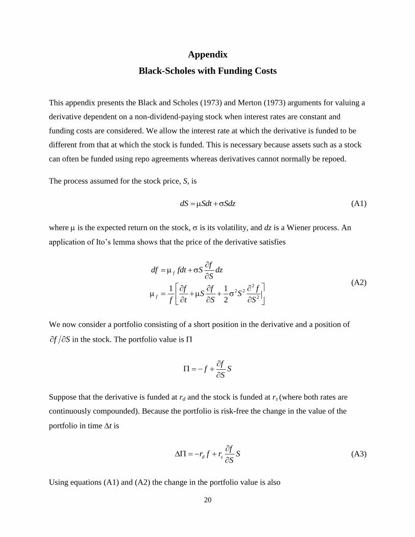
Appendix

Black-Scholes with Funding Costs

This appendix presents the Black and Scholes (1973) and Merton (1973) arguments for valuing a

derivative dependent on a non-dividend-paying stock when interest rates are constant and

funding costs are considered. We allow the interest rate at which the derivative is funded to be

different from that at which the stock is funded. This is necessary because assets such as a stock

can often be funded using repo agreements whereas derivatives cannot normally be repoed.

The process assumed for the stock price, S, is

dS Sdt Sdz (A1)

where is the expected return on the stock, is its volatility, and dz is a Wiener process. An

application of Ito’s lemma shows that the price of the derivative satisfies

2

2 2

2

1 1

2

f

f

fdf fdt S dz

S

f f fS S

f t S S

(A2)

We now consider a portfolio consisting of a short position in the derivative and a position of

Sf in the stock. The portfolio value is

f

f SS

Suppose that the derivative is funded at rd and the stock is funded at rs (where both rates are

continuously compounded). Because the portfolio is risk-free the change in the value of the

portfolio in time t is

d s

fr f r S

S

(A3)

Using equations (A1) and (A2) the change in the portfolio value is also

21

2

2 2

2

1

2

f fS t

t S

(A4)

Combining equations (A3) and (A4) leads to the differential equation

frS

fS

S

fSr

t

fds

2

222

2

1

The risk-neutral valuation argument shows that the solution of this differential equation is

obtained by assuming that the expected return on the stock is sr and then discounting the

expected payoff at dr . For a derivative that provides a payoff only at time T

PEefTrd ˆ

0

where 0f is the derivative price today (time zero), P is the payoff at time T, and E denotes

expectations in a world where the expected growth rate of the stock price is rs. The value of a

European call option on the stock with strike price K and time to maturity T is

)()( 2

)(

10 dNKeedNSTrTrr dds

where

Tdd

T

TrKSd s

12

2

01

)2/()/ln(

These results can be extended to derivatives dependent on assets other than non-dividend-paying

stocks.