“The siting of large-scale livestock facilities near homes disrupts rural life as the freedom and independence associated with life oriented toward the outdoors gives way to feelings of violation, isolation, and infringement.”

--Pew Commission on Industrial Farm Animal Production

Valuing Localized Externalities:

Hog Operations in North Carolina

Sara Murray∗

Duke University

Durham, NC

April 2009

Professor Christopher Timmins, Faculty Advisor

∗ Sara Murray graduated in May 2009 with High Distinction. This thesis was a co-winner of the Best Honors Thesis prize. Sara can be reached at saradmurray@gmail.com

2

Acknowledgments

I am especially grateful to my thesis advisor, Professor Christopher Timmins, for

his dependable advice, patience with my constant emails, and support throughout this

year. I am also incredibly grateful to my Econ198S and 199S professor, Peter

Arcidiacono, for his guidance and insightful feedback during the research and writing

process. I would also like to thank my fellow seminar classmates for their helpful

comments on drafts and presentations. Special thanks to Joel Herndon, Mark Thomas, and

Tatyana Kuzmenko for their invaluable computer expertise and assistance.

3

Abstract

In the early 1990s, eastern North Carolina experienced a boom in industrial hog

production. Among the negative externalities generated by this activity, residential

property value losses due to operation proximity are some of the most significant. This

paper discusses the impact of hog operation presence on median housing values for census

tracts and blocks (the smallest geographic unit the Census Bureau keeps data on). It

concludes that measuring localized externalities at the tract level yields insignificant

results, but that measuring these at the block level accurately shows the marginal impacts

on housing values. At ½ kilometer, one operation can cause a 9% decline in value, or a

drop equal to almost $7,000 in magnitude. Even without considering health, sociological,

and political consequences, the economic drawbacks from these industrial-sized animal

feeding operations gives a substantial reason to re-evaluate their siting, expansion, and

ultimate necessity.

4

I. Introduction

Locally undesirable land uses, such as power plants, hazardous waste sites, and

animal feeding operations, have become a nuisance in rural areas across the country.

Waste materials from these facilities contaminate the surrounding air and water, usually

leaving nearby residents with no compensation. Even though measuring the damage from

these facilities can prove difficult, most research has found that health, social, and

economic effects are negative in a localized area (within a couple of kilometers).

Measuring economic externalities is made possible by house price capitalization, whereby

the value (or disvalue) of an environmental characteristic can be extracted from its

contribution to the value of a house.

One type of locally undesirable land use, confined animal feeding operations,

congregates “animals, feed, manure and urine, dead animals, and production operations on

a small land area,” and produces a host of negative externalities (Environmental

Protection Agency, 2009). Specifically, in North Carolina, industrial hog production has

become increasingly concentrated into smaller geographic areas so that the economic

effect of these facilities shows up in decreased housing values for those residents nearby.

The North Carolina hog industry has surpassed the tobacco industry in terms of the

agricultural income that it generates for the state. North Carolina produces 19% of the

total United States hog output, valued at over $2 billion, and ranks second only to Iowa.

Corporations have touted the economic benefits of large-scale hog operations: greater tax

revenues, more local products, job creation, and increased organic plant nutrients for crop

production. During the pivotal decade of the 1990s, the North Carolina hog industry grew

from 2.6 million hogs to almost 10 million today (Environmental Defense Fund). The

5

industrialization of the industry that began in the late 1980s continued uninhibited well

into the 1990s because local environmental groups began to take action only after major

polluting incidents (Furuseth, 1997).

Manure disposal poses one of the greatest environmental challenges for the

industry. The average total waste generated by hogs in North Carolina per day is thirteen

million pounds (Duke Department of Sociology). Traditionally, farmers use open-air

anaerobic lagoon pits to contain the waste. Ammonia and methane emissions may drift

into the air of surrounding neighborhoods (EDF). Foul odors can spread for miles, excess

nutrients may seep into and contaminate ground and surface water, workers may develop

respiratory ailments, and toxins from waste can create health hazards for residents situated

nearby. This paper tests for a negative relationship between median housing prices (at

both the census tract and block level) and hog operations in order to measure the localized

externalities.

Much debate still exists surrounding the level at which to measure localized

externalities in hedonic analysis, so this paper uses both census tracts and blocks. Some

studies use county-level data, while others use individual house prices. I use both tract-

level and confidential block-level data, to see how the relationship changes with the level

of geographic aggregation. My data contain information for the years directly before the

boom in hog production and directly after, and should be able to fully capture any effects

on housing values.

Coefficients on hog operation presence are negative and significant using the

block-level data, while the coefficients at the tract level are not significant. In terms of

magnitude, one hog operation located at ½ kilometer from a house can lower the house’s

6

value by as much as $6,968. Knowing this information has useful implications for

homeowners seeking damages and for policy makers deciding questions of industry

expansion. Most importantly, my results show that using the most geographically-specific

Census Bureau data available captures the extent of damages caused by very local

undesirable land uses.

This paper is divided into five sections. Section II reviews relevant literature that

has examined the impact of different types of locally undesirable land uses on residential

property values. Section III discusses the sets of data used: Dun and Bradstreet data on

hog operations back to 1990, census tract data from 1990 and 2000, and census block data

from 1990 and 2000. Section IV discusses the theoretical framework of hedonic analysis

as applied to housing values and the empirical methods used. Section V presents the

results of tract-level and block-level analysis. The final section concludes the paper and

discusses areas for future research.

7

II. Literature Review

While there have been a great number of studies conducted on measuring localized

externalities, there has been limited research conducted on the effects of swine operations

on residential housing values. None of the previous studies on confined animal feeding

operations has used census block data, and none has tracked changes in housing values

over time. Instead, most of the studies have combined data on housing sales with varying

data on animal-herd numbers to run cross-sectional regressions. They have found mixed

results depending on distance, operation concentration, and operation size.

The most well-known and comprehensive study, conducted by Palmquist, Roka,

and Vukina used data on 237 home sales in the early 1990s, and data on the total number

of herds within specified distance rings around each house because they did not have data

on exact hog operation locations. A “herd” is one hog or more, so they used “market-herd

equivalents” to develop a manure index as well. They found that “if a new operation

locates within one-half mile of a house…house value drops by 4.75%” (Palmquist et al.,

1997). The drop in value is dependent upon manure levels and previous concentration of

operations in the area. Overall, they found that operation proximity does have a negative

and significant impact on property values (Palmquist et al., 1997). They admit, however,

that “data on hog farm locations would allow the inclusion of important variables such as

exact distances between farms and residents” (Palmquist et al., 1997). I expand on their

research by using data from thousands of housing values (instead of sales) after the boom

in hog production, and data containing the precise location of the operations (exact

latitudes and longitudes).

8

A more recent study on the topic is titled “Living with Hogs in Iowa: The Impact

of Livestock Facilities on Rural Residential Property Values” by Herriges, Secchi, and

Babcock. In this study, the authors used county assessor data on home sales (over 1,000)

and the exact location and size of livestock feeding operations in five rural counties. They

found that “predicted negative effects are largest for properties that are downwind and

close to livestock operations” (Herriges et al., 2003). They also counter-intuitively found

that “feeding operations that are moderate in size have more impact than do large-scale

operations, most likely reflecting age, type, and management practices of the moderate-

sized operations” (Herriges et al., 2003). These authors used GIS data on the location of

livestock facilities, but did not use panel data. They constructed centroids for property

sales and livestock operations, and calculated distances between the two (Herriges et al.,

2003). I use a similar technique by constructing centroids for census blocks and measuring

the concentration of hog operations within specified distance rings.

Gallagher and Greenstone used census tract data and GIS techniques in their study

titled “Does Hazardous Waste Matter? Evidence from the Housing Market and the

Superfund Program.” They used census tract data to estimate the local welfare impacts of

hazardous waste site clean-ups. They showed that waste site clean-ups are associated with

a small and statistically insignificant change in property value (Greenstone and Gallagher,

2008). My results show a similar story at the tract level, suggesting that this level of

analysis is too large to measure localized externalities. The authors used GIS to draw

circles around each Superfund site and incorporated data from all tracts that fell within a

certain radius to calculate demographic and housing values. I perform a similar analysis at

9

the block level by drawing radii around each centroid and counting the number of

operations contained.

Glenn Blomquist’s approach in the “Effect of Electric Utility Power Plant

Location on Area Property Values” (1974) guided the (cross-sectional) census block

portion of my research. I use the same dependent variable: mean property value (the block

average of owners’ estimates of market sale price of house and lot for all owner-occupied,

single family dwelling units). He also mentions that zoning requirements are believed to

limit too much variation in lot size - this makes using census block data less prone to

omitted variables bias. He measured distance to power plants as the distance from the

center of the block to the smokestack of a power plant, showing that this empirical method

can correctly measure localized negative externalities.

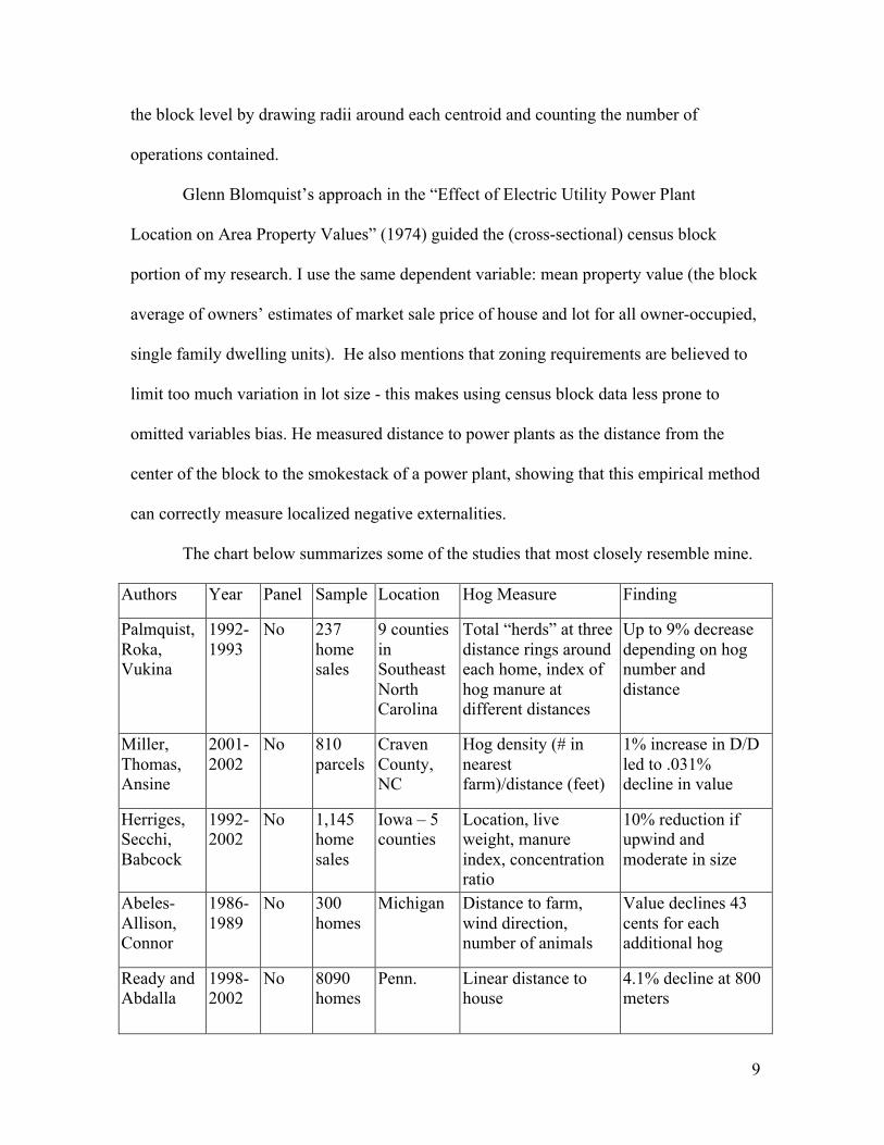
The chart below summarizes some of the studies that most closely resemble mine.

Authors Year Panel Sample Location Hog Measure Finding

Palmquist, Roka, Vukina

1992-1993

No 237 home sales

9 counties in Southeast North Carolina

Total “herds” at three distance rings around each home, index of hog manure at different distances

Up to 9% decrease depending on hog number and distance

Miller, Thomas, Ansine

2001-2002

No 810 parcels

Craven County, NC

Hog density (# in nearest farm)/distance (feet)

1% increase in D/D led to .031% decline in value

Herriges, Secchi, Babcock

1992- 2002

No 1,145 home sales

Iowa – 5 counties

Location, live weight, manure index, concentration ratio

10% reduction if upwind and moderate in size

Abeles-Allison, Connor

1986-1989

No 300 homes

Michigan Distance to farm, wind direction, number of animals

Value declines 43 cents for each additional hog

Ready and Abdalla

1998-2002

No 8090 homes

Penn. Linear distance to house

4.1% decline at 800 meters

10

None of the previous studies has all of the following: 1) a very large sample size 2)

panel data and 3) precise measures of location. While there are not a large number of

studies conducted specifically on hog operations, the literature estimating the effects of

localized environmental externalities is extensive enough to guide my research on swine

operations and rural residential property values in North Carolina. Most previous studies,

however, were conducted before or during the boom in hog production, and do not use a

panel dataset to measure changes over time. My panel dataset contains information on

both census blocks and tracts in the largest hog producing counties in North Carolina. My

hog operation data contain information on exact operation locations, employees, and sales.

Using confidential block data from two points in time and employing fixed effects to

control for omitted variables, I determine the precise magnitude of the negative effect of

operations on a very detailed level.

11

III. Data

Coastal Plains North Carolina is an important study location because of its

comparative advantage in swine production due to poor soil resources, strong government

support, comparatively few environmental regulations, proximity to East coast markets,

and lower on-farm production costs (The Pig Site). Throughout the 1990s, hog farming

became increasingly concentrated in narrower geographic areas. The facts below

summarize the trends:

• From 1989 to 1995, the percentage of the state’s hog population in ten Coastal Plains

counties jumped from 39% to 67%

• By 1992, over 90% of the swine population was concentrated on just 802 farms

• In 1998, 92% of the states’ 10 million hogs were raised on operations of at least

2,000 head (North Carolina Coastal Federation)

Hog Operation Data

My data on hog operations come from Dun and Bradstreet, a corporation whose

database contains quality business information, services, and research on companies. The

data contain not only information on the exact location of hog operations (geographic

coordinates), but also figures for the number of employees and the amount of sales in each

year beginning in 1990. It also contains yearly entry and exit information for each firm.

The Dun and Bradstreet hog data match the trends in the industry as described by

current literature. In 1995, the Swine Farm Siting Act required waste lagoons and hog

houses to be situated 1,500 feet from any occupied residence but only on all new or

expanded hog farms raising more than 250 hogs. Most importantly, in 1997, House Bill

515 imposed a moratorium on the construction of new and expanded hog operations with

12

250 or more hogs until March 1, 1999 as well as imposed an additional setback

requirement for hog houses and lagoons to 2,500 ft (Environmental Defense). Owen

Furuseth found that the “ten counties of southeastern North Carolina captured 78% of the

statewide expansion in swine populations during the past six years…In 1989 these

counties contained slightly more than 39% of North Carolina’s hog population (1.2

million head), but by 1995 their share had jumped to 67% (4.4 million animals)”

(Furuseth, 1997). See Charts 1-3 in the Appendix to observe the trends as described by my

data.

According to my data set, until 1997-1998, the total number of employees steadily

increased, then leveled off. The total number of firms increased linearly throughout the

decade. This is consistent with the observed decline in total number of hog farms across

the entire state: my data captures only the explosion in production in the eastern portion of

the state. Interestingly, average sales increased throughout the decade as expected, then

precipitously declined after 1997. To evade the moratorium, farmers constructed smaller

operations: this neatly explains both the trend of increasing firms and the trend of

decreasing average sales. These three charts clearly capture the apparent trend in the

industry over the decade.

In most recent studies of the effect of confined animal feeding operations, the size of

the herd or pounds of manure is used as the independent variable to serve as a proxy for

negative externalities. The problem with this approach is that in some cases, “larger

operations…tend to be newly built and employ best available technologies for dealing

with waste and odor” (Putze). I do not have data on prevailing wind directions, size of the

associated waste lagoons, water quality, or number of swine contained in each operation. I

13

rely on the simple existence of a swine facility to measure its effects, and omit distinctions

between small and large operations.

Housing Data

Data on median housing characteristics are drawn from the United States Census

Bureau. First, I utilize census tract variables from both 1990 and 2000 for the largest hog

producing counties in North Carolina: Beaufort, Bladen, Columbus, Craven, Duplin,

Edgecombe, Greene, Halifax, Harnett, Johnston, Jones, Lenoir, Nash, Northampton,

Onslow, Pender, Pitt, Robeson, Sampson, Warren, and Wayne. The darkest color in

Figure 1 depicts the largest hog producing counties in the state, all located in

southeastern North Carolina.

FIGURE 1: Largest Hog Producing Counties in North Carolina

A census tract is a small statistical subdivision of a county. Tracts generally

contain information for 2,500-8,000 people and, when first delineated, “are designed to be

homogeneous with respect to population characteristics, economic status, and living

conditions” (Census Bureau). This implies that in rural areas, such as Coastal Plains North

Carolina, tracts will cover a relatively large geographical area. The Census Bureau

collects the following information for each tract: median household income, median

property value, median number of rooms per house, house age, ethnicity percentages,

Source: North Carolina Department of Agriculture

14

mean travel time to work, percentage of the population over 25 with a bachelor’s degree,

etc. All of these variables will impact housing values and need to be controlled for in any

analysis.

The median housing values are owner imputed. Champ, Boyle, and Brown state

that homeowner surveys of value are one commonly used method of collecting data on

property values, with the only caveat that measurement error may be a significant concern.

Owners’ lack of information about neighborhood amenities might cause them to

overestimate or underestimate the value of their houses for different purposes. In the

census survey, housing value is not a continuous variable, and the participants could not

answer the valuation question with “I don’t know.” County appraisers are required to

consider the impacts of contamination and other externalities in the value estimation

process, but owners are not (Kilpatrick, 2001). Because repeat sales data in rural areas is

very difficult to obtain and because the turnover of houses is relatively infrequent (causing

spatial imbalance), I use median housing values (Kim and Goldsmith, 2007). The two

greatest benefits of using median housing values are that I utilize an incredibly large

sample size and account for all houses in the study area.

Using Geolytics’ Neighborhood Change Database, it is possible to compare census

tracts across time, even though the delineated boundaries of the tracts may have changed

significantly. The software takes the 1990 Census Bureau information but uses 2000 tract

boundaries to recalculate the population and housing figures so that 1990 and 2000 tracts

can be compared. Below are means for census tract data, with dollar amounts adjusted for

inflation.

15

TABLE 1: Tract Means, 1990 and 2000

As the table above shows, from 1990 to 2000, the average census tract population

grew 18%: from 4,801 to 5,644. The mean number of hog operations grew from 0.95 in

1990 to 1.6 in 2000. This is a 68.4% increase, suggesting a very high level of overall

growth in the hog industry. I calculated the inflation rate across the decade as 31.8%, and

reported all monetary variables in $2000. Real median household income increased from

$28,166 to $38,274, which is consistent with the general increase in the rest of the

country. Finally, real median housing value increased from $68,077 to $81,164. This is

also expected, as the 1990s witnessed one of the greatest housing booms in the century.

Most of the variables (number of bedrooms per house, percentage of the population with a

Bachelor’s degree or higher, percentage of mobile homes, percentage of houses that are

owner-occupied, percentage below the poverty line) remained very similar over the

decade, due to the homogeneous nature of eastern North Carolina. Overall racial

Variable Mean 1990 Mean 2000 Tract Population 4801 (1,926) 5644 (2,700) Percentage of Owner Occupied Houses

0.60 (.15) 0.59 (.16)

Median Household Income ($) 28,166 (9,058) 38,274 (8,825) Average Household Income ($) 35,895 (9,364) 40,772 (9,478) Percentage of Mobile Homes 0.19 (.12) 0.22 (.14) Percentage of Population with a Bachelors Degree +

0.11 (.08) 0.14 (.09)

Percent Below Poverty Line 0.19 (0.09) 0.19 (0.09) Median Property Value (all $2000)

68,077 (29,290) 81,164 (22,853)

Hog Operations 0.95 (1.77) 1.6 (2.77) White 0.62 (.23) 0.58 (.23) African-American 0.34 (.22) 0.35 (0.22) American Indian 0.03 (0.12) 0.03 (0.11)

Note: Standard deviations are listed in parenthesis next to each mean. The inflation rate used was 31.8%.

16

demographics changed very little. See Table 3 in the Appendix for tract means broken out

by high-growth and log-growth hog counties.

Census blocks are “the smallest geographic area for which the Bureau of the

Census collects and tabulates decennial census data” (Census Bureau). These data contain

information on a much smaller subdivision of the tracts (on the order of around 250-550

housing units). The nature of the blocks allows me to calculate changes in housing value

on a much smaller and more precise level than is possible using tracts.

These datasets are very appropriate for studying the effects of operations on

housing values in eastern North Carolina because hog operations started to grow most

significantly during the 1990s. Even though many of the operations started before 1990,

residents in the area would have been less aware of associated externalities due to the

operations’ smaller presence. By analyzing data before the appearance of large,

concentrated hog farms and comparing it to data a decade later, there should be clear,

observable effects on housing values situated near those operations.

Because my data give the year that each operation started, it is possible to determine

the exact tract that a hog operation lies in by entering in its latitude and longitude in

ArcMap software. Using this method, I counted the number of operations contained

entirely within each tract in 1990 and 2000. See Table1 in the Appendix for operation

percentiles. The median number of operations per tract was 0.95 in 1990 and 1.64 in 2000.

I then counted the number of operations contained within varying radii of each block

centroid for 1990 and 2000. See Figure 2 below for the average of these counts for

selected distances.

17

FIGURE 2: Average Operation Count Per Block

As expected, the number of operations increased as the included distance around each

block centroid increased. The average number of operations in 2000 was greater than the

average number in 1990 at all distances.

0 

1 

2 

3 

4 

5 

6 

0.50  1  2  3  4  5  10 

Operation Count 

Distance (km) 

Average Operation Count Per Block 

1990 Average 

2000 Average 

18

IV. Theoretical Framework and Empirical Specification

To conduct this research, I follow methods of previous research on localized

externalities by applying the fundamentals of house price hedonic analysis. Hedonics have

become the gold standard for measuring the effects of specific characteristics on housing

values. Housing is a heterogeneous good: a “product whose characteristics vary in such a

way that there are distinct product varieties even though the commodity is sold in one

market” (Champ, Boyle, Brown, 2003). These goods have a common price structure

because their attributes comprise similar, but not identical, parts. The value of a house is

generally written as a function of various attributes:

Value = V(x1, x2, … , xn) where x = (x1, x2, ... , xn) is a vector of housing attributes.

Implicitly included in the value of a house are environmental variables that cannot

be measured directly. Environmental amenities are generally thought of as non-marketable

goods (clean air and water cannot be traded in a market). For this reason, economists use

hedonic estimation by assuming that consumers implicitly buy an environmental good

when they purchase a marketed good, such as a house (Boyle and Kiel, 2001). A house is

made up of structural, neighborhood, and environmental characteristics, all of which are

capitalized into the house’s value. Examples of structural characteristics include: house

age, median number of rooms, number of bedrooms, and heating method. Neighborhood

and environmental characteristics may include: median household income, race, education

levels attained, distance to work, and quality of environmental amenities. Because census

data contain very limited amounts of information on structural housing characteristics, I

will rely mainly on neighborhood characteristics for the tract analysis.

19

Regressing characteristics of a good on the value of that good (the house), we can

extract the contribution of the environmental good to the value of the marketed good

(Boyle and Kiel, 2001). This theoretical framework informs my empirical specification by

suggesting likely explanatory variables and equational forms.

When using census tract data, I use only the concentration of hog operations in

each tract as an independent variable to determine the impact of these negative

externalities. When using census block data, however, I draw rings around each census

block centroid and determine how many operations lie within certain radii of the centroid.

Hedonic models are generally estimated using ordinary least squares. I use both

linear and logarithmic specifications. One basic cross-sectional equation with hog data to

be estimated is as follows:

€

Ln(MedianValue)it =α0 + β1HogOperationCountit + β2PctMobileit + β3AfricanAmericanit+β4AmericanIndianit + β5Electricityit + β6Ln(MedHHIncit ) + β7Bedroomsit + εit

(1)

Willingness to pay (WTP) for a given characteristic can thus be valued by taking

the partial derivative of the median house value with respect to a characteristic:

€

WTPi = ∂MedianValuei /∂HogOperationCounti (2)

Each coefficient represents the marginal contribution of the attribute to the house

value. My null hypothesis is that there is no significant association between median

housing value and hog operation concentration (B1=0). The alternative hypothesis is that

the coefficient on hog operations will be negative and significantly different from 0.

20

Usually the price of a house (the dependent variable) is specified in semi-log form, which

“allows for variation in characteristic prices across different price ranges within the

sample” (Sirmans et al., 2007). This is relevant to my dataset because housing values

range widely across the study area.

In a second specification, I perform a time-series analysis and control for the

presence of other locally undesirable land uses that could also impact housing values by

using county, tract, and block fixed effects. Fixed effects coefficients “soak up” all the

across-group variation (Dranove, 2009). These control for time-invariant neighborhood

characteristics by focusing on housing value changes over time, using a difference-in-

difference approach (Davis). I assume that any macroeconomic exogenous changes

affected all areas of eastern North Carolina equally. My fixed-effects specification is:

€

ΔLogMedValuei =α0 + β1ΔOperationsi + β2ΔAfricanAmericani + β3ΔBedroomi

+β4ΔLogMedHHInci + β5ΔElectricityi +Vi + εi (3)

Problems may arise if unobservable characteristics do change over time.

When using block data, I utilized similar independent variables, but instead of

including an independent variable for number of operations within each block, I count the

number of operations within a specified distance of each block centroid. This overcomes

the problem of having features of surrounding blocks being important property value

predictors for a nearby block. Using Matlab, is it possible to draw circles around each

block centroid and count the number of operations within various chosen radii. The most

appropriate method of performing these calculations is done using the Great Circle

21

Distance formula, which takes two pairs of latitudes and longitudes (one from block

centroids and one from hog operations) and draws a circle of a specified radius around a

block centroid. The formula is:

€

D = arccos(sin(lat1) × sin(lat2) + cos(lat1) × cos(lat2) × cos(long2 − long1))× R (4)

Equation 4 takes into account the spherical nature of the earth’s surface and is thus very

precise in measuring distances. Using operation counts around each centroid, I run cross-

sectional and time-series regressions similar to the tract analysis.

22

V. Results

a. Census Tracts

The hog industry has changed from an abundance of small family farms to a

concentration of gigantic swine operations. Abeles-Allison and Connor find that “one

thousand hogs result in a drop of $430 in property value on a single property” for a five-

mile radius around the house (Abeles-Allison and Connor, 1990). They also find that

“larger hog operations have a greater impact than do smaller ones” (Abeles-Allison and

Connor, 1990). Palmquist et al. suggest that “proximity caused a statistically significant

reduction in house prices of up to 9% depending on the number of hogs and the distance

from the house” (Palmquist et al., 1997). I compare my results at the tract level to these

two studies. The results of the 2000 cross-sectional and fixed-effects regressions using

census tracts is below:

Variable (1) 2000 Cross-Section

(2) 1990 Cross-Section

(3) Fixed Effects

Intercept Ops00 Percent Built Last 5 Years Percent Mobile Percent African-American Percent American Indian Percent with 0-2 Bedrooms Log Median Household Income Percent with Electricity

5.81** (0.66)

0.00075 (0.0037) 0.676** (0.183)

-0.404** (0.122)

-0.318** (0.058)

-0.256** (0.095)

-0.358** (0.108) 1.23** (0.137) 0.147* (0.068)

3.16** (0.59)

-0.0041 (0.005)

-0.323** (0.114) 0.089

(0.079) -0.02 (0.12) 0.365* (0.15) 1.73** (0.12) 0.40** (0.091)

-0.028 (0.0278)

.0091 (0.008)

0.721** (0.224) -0.264 (0.224) 1.72*

(0.922) -0.778** (0.217) 1.176** (0.109) 0.152

(0.159) Number of Observations

Adjusted R^2 249 .67

249 0.62

248 0.36

TABLE 2: Tract-Level Analysis, and Fixed Effects

23

In both 1990 and 2000, the coefficient on hog operations was not significant. Other

explanatory variables, such as the percentage of houses with electricity, the logarithm of

median household income, and the percentage of mobile homes all significantly affected

housing value in the expected direction in the cross-sectional models. The adjusted R2 was

0.67 and 0.62 for 1990 and 2000, respectively, indicating that a majority of the variance in

housing value was explained by the model. In the panel regression, fewer explanatory

variables were significant. Most importantly, the coefficient on change in hog operations

is insignificant.

These results comprise the first segment of my research using tract data. In neither

the cross-sectional regressions nor the panel regression did hog operations influence

housing values significantly. Using a linear regression model and a semi-log model with

different independent variables did not change the outcome: hog operations do not appear

to be significantly related to housing prices at the tract level. I hypothesize that this does

not mean that hog operations do not impact housing value, but rather that hog operations

produce such a localized externality that tracts are too large a geographic unit at which to

identify their impact. My results fit with what Ann Ulmer and Ray Massey describe in

their summary of CAFO impacts on housing values, that “ the impact of AFOs [animal

feeding operations] on property value [is] localized or limited to properties near the AFO”

(Ulmer and Massey, 2008). The effect of a hog operation is likely to affect only a very

small percentage of the tract area, making it very difficult to determine the effect on

Note: Dependent variable is the logarithm of median property value for the tract. Standard errors are in parenthesis. An * indicates significance at the 5% level, a ** indicates significance at the 1% level.

24

median housing values in a miles-wide tract. Using block data overcomes this problem

and yields much more accurate results.

b. Census Blocks

I hypothesize that hog facilities closest to census block centroids would negatively

impact block median housing values. I expect the coefficients on kilometer radii to enter

the regression negatively, and become less negative at greater distances as the externality

dissipates. Having data on median housing value changes in areas with no operations

serves as a baseline comparison. If values either increase or decrease significantly in

blocks near many facilities, I can assume the value change is due to operation presence, as

little else in the economy is likely to have changed over this period.

First, I run cross-sectional regressions using 1990 and 2000 census block data

merged with hog operations counts using radii from 0.5 kilometers up to 5 kilometers

around the centroid of each block. Included in these regressions are more explanatory

variables than I included in the tract regressions, such as the median number of bedrooms,

housing unit density, and the share of houses with incomplete plumbing. Secondly, I run

panel regressions that control for unobserved variables that may differ across blocks but

stay constant over time. See Table 3 for a comparison of the coefficients. This table shows

a comparison for ½ kilometer only, because each of the 3 models at varying distances

remained almost identical.

25

TABLE 3: Block-Level Analysis, and Fixed Effects

In both specification (1) and (2) – the cross sections - the coefficients on hog

operation count at distances of up to at least 5 kilometers were all significant and negative.

In 1990, the median house value was expected to be 4.4% lower for each additional

operation within ½ kilometer. In 2000, the median house value was expected to be 9%

lower. The magnitude of these coefficients decreased (become less negative) as the

kilometer distances increase. As expected, at further distances operations impact housing

values less. All other variables are significant and have the expected sign. For these two

Variable (1) 1990 ½ Km

(2) 2000 ½ Km

(3) Fixed Effects ½ Km

Intercept Distance (Km) Percent Mobile Percent Plumbing Median Bedrooms Percent African-American Percent American Indian Percent BA+ Housing Density Ln(Median Household Income) Observations R2

9 (.046) -.044** (.008) -1.2** (.012) .12** (.024) .077** (.0046) .36** (.009) -.38** (.02) .49** (.013) 0** (0) 0.10** (.004) 26,365 0.47

9.0 (.077) -0.09** (.017) -0.834** (.012) .182** (.059) .205** (.0065) -0.273** (.013) -.321** (.0283) .397** (.0173) -0.00** (0) .151** (.0054) 262,520 0.37

.234 (.0078) -0.0071 (.015) -0.77** (0.019) 0.194** (.039) 0.092** (.0062) -0.214)** (0.027) -0.06 (.095) 0.138** (.019) 1.0e-06 (1.02e-07) 16,787 0.13

Note: A ** indicates significance at the 1% level. A * indicates significance at the 5% level. The dependent variable for models (1) and (2) was the logarithm of median housing value, and the dependent variable for model (3) was change in the logarithm of median housing values.

26

specifications, the semi-log model produced the best results. The results also fall within

the range of what previous cross-sectional work has found.

The figure below shows the point estimates for all kilometer distances up to 5

kilometers in 1990 and 2000. The dark line, representing 2000, lies above the 1990

estimates at all values until 4 kilometers. These coefficients imply that after the expansion

and construction of hog operations throughout the decade, those who lived closest felt the

negative externalities more acutely. If there is an increasing marginal effect, then the

increase in number of operations would also increase the effect across the decade.

FIGURE 3: Point Estimates of Hog Operation Distance Coefficients, Cross Sections

In terms of actual magnitudes, housing value decreases $6,968 at ½ kilometer

radius in 2000. The figure for 1990 is $4,307 after adjusting for inflation. With a sample

of 22,520 houses in 2000 this amounts to a total property value loss of at least $156, 919,

360. In reality this figure is much larger because the sample of 22,520 is much smaller

than the total number of observed houses (over 50,000) in the twenty two counties I

‐0.14 

‐0.12 

‐0.1 

‐0.08 

‐0.06 

‐0.04 

‐0.02 

0 0  1  2  3  4  5  6 

Elasticity 

Distance (Km)  

Semi­Log Estimates of Median Housing Value With Respect to Hog Operations 

1990 

2000 

27

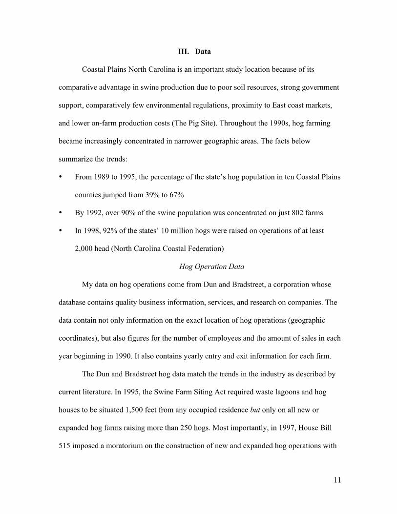
gathered data for. Even at a distance of four kilometers one operation can lower value by

$1,039. One operation therefore may not have a significant effect in terms of magnitude,

but as more operations locate in close proxmity to a house, the more severly a house’s

value will be affected. Figure 4 shows magnitudes for the panel dataset.

FIGURE 4: Point Estimates of Hog Operation Distance Coefficients, Panel

In Figure 4, all point estimates of housing value change were negative, but only

some were significant. The ones that were significant had a much smaller magnitude

than those in the cross-section. These estimates are conservative, but the results suggest

that at 1.5, 2, 3,4, 5 kilometers, all coefficients were significant at the 1% level. For the

cross-sectional models, the semi-log model produced the best results, however, running

the panel regressions with actual median housing value change produced the best

results. Even after controlling for unobserved variables in the panel regression, I still

find a negative effect. The effect decreases in magnitude from the cross-sectional

regressions, but it is still significant and suggests that hog operations affected value.

‐4500 ‐4000 ‐3500 ‐3000 ‐2500 ‐2000 ‐1500 ‐1000 ‐500 

0 500 1000 1500 

0  1  2  3  4  5  6 

Point Estimates ($) 

Distance (km) 

Linear Estimates of Median Housing Price Change With Respect to Change in Hog Operations 

Fixed Effects Value 

28

The results are not surprising. It seems that in 1990, the majority of farms in

eastern North Carolina all raised a small number of hogs. By the end of the decade

industry expansion had taken off, and the farms that chose to specialize in hogs

increased their farm capacity by the thousands. Residents living in the area in 1990

would have been unlikely to be upset with small farms containing a small herd of hogs.

Residents living in the area in 2000, however, would have been much more likely to

notice the effects of gigantic facilities emitting odors and thousands of pounds of

manure each day. Most likely, the increase in facility number and the increase in hog

concentration caused the increase in the magnitude of the coefficient on operation

counts over the decade.

29

VI. Conclusions

In my research, I draw and expand upon the conclusions reached by previous

researchers by using a more up-to-date detailed dataset, incorporating GIS techniques, and

extending analyses from different areas of the United States to an expansive area in North

Carolina. I found inconclusive results when using data from the census tract level, and

found conclusive results using census block data, as census blocks are much more precise

geographic areas and have more homogenous demographic and housing characteristics. In

both 1990 and 2000, hog operations negatively impact median housing values in blocks

with higher numbers of hog operations in the vicinity.

This has important implications for the hog industry, policy makers and regulators,

and researchers. Clearly, those individuals living in closest proximity to the facilities

notice their environmental damages, and these damages can be quantified into monetary

terms. Specifically, one operation located within one kilometer of a home caused a $5,057

decline in value in 2000. Controlling for unobserved variables over the decade, the decline

in value was $1,495 at 1½ kilometers, significant at the 5% level. Having solid economic

data to back up their complaints, homeowners will be able to protest expansion and

construction of hog facilities. Using these results, policymakers may impose stricter

regulations on operations, impose a tax per animal to generate revenue to compensate

residents for living near hogs, or force operations to adopt cleaner waste management

technologies.

My results are also important in terms of research methods. Studies conducted at

large heterogeneous geographic areas, such as counties and tracts, may not accurately

capture the benefits or drawbacks of specific types of land uses. Block-level data, though

30

difficult to obtain, yield much more significant results. Census Bureau data in general,

with large sample sizes across time, allow for a more comprehensive analysis than is

possible using individual housing sales and selected hog operations.

My results support and confirm earlier findings on the loss of housing value due to

hog operation proximity. Palmquist, Roka, and Vukina find that rural residential property

values decrease 9% if an operation locates within ½ mile. Similarly, I found that at ½

kilometer, housing values decline by 9% as well, in 2000. Palmquist et al.’s article was

published before the swine lagoon ban in 1997, yet my results show that the ban did not

impact housing values in a positive manner.

In 2007, North Carolina was the first state to ban the construction and expansion

of new lagoons and spray fields by passing the Swine Farm Environmental Performance

Standards Act. In that year, policymakers made serious reforms regarding the waste

problem. This act sets strict standards for any new waste management system (EDF). An

interesting area for future research would involve using 2010 census block data to

determine if this Act caused a significant decline in the amount of negative externalities

produced by waste lagoons, leading to a corresponding rise in house values.

My research shows that using information from 250 census tracts and over 50,000

census blocks in an expansive area of North Carolina produces a picture of how localized

externalities can impact the value of residential property. It would be interesting to extend

this analysis to other forms of confined animal feeding operations to see if the results are

as conclusive.

31

Works Cited

Environmental Defense. (2007, August). 2007 NC Swine Farm Environmental Performance Standards Act. Retrieved from http://www.edf.org/documents/6979_NC_Swine_Performance_Act.pdf

Abeles-Allison, Mark and Larry J. Connor. (1990). An Analysis of Local Benefits and

Costs of Michigan Hog Operations Experiencing Environmental Conflicts. Agricultural Economics Report #536. Department of Agricultural Economics. Michigan State University.

Blomquist, Glenn. (1974). The Effect of Electric Utility Power Plant Location on Area

Property Value. [Electronic version]. Land Economics, 50(1). Boyle, Melissa and Katherine Kiel. (2001). A Survey of House Price Hedonic Studies of

the Impact of Environmental Externalities. [Electronic version]. Journal of Real Estate Literature, 9(2). Champ, Patricia, Boyle, K., and Brown, T. (2003). A Primer on Nonmarket Valuation. Boston: Kluwer Academic Publishers. Chay, Kenneth and Michael Greenstone. (2005). Does Air Quality Matter? Evidence from

the Housing Market. [Electronic version]. Journal of Political Economy, 113(2). Davis, Lucas. (2008, June). The Effect of Power Plants on Local Housing Values and

Rents: Evidence from Restricted Census Microdata. U.S. Census Bureau Working Paper 08-19.

Dranove, David. (2009). Fixed Effects Models. [PDF document]. Retrieved from

http://www.kellog.northwestern.edu/faculty/dranove/htm/Dranove/coursepages Duke University Department of Sociology. (2007). North Carolina in the Global

Economy: Hog Farming. Retrieved from http://www.soc.duke.edu/NC_GlobalEconomy/hog/overview.shtml.

Dun and Bradstreet. (2009). National Establishment Time-Series Database. Available

from http://www.dnb.com/us/ Environmental Defense. (2002). Major North Carolina Laws Related to Hog Factory

Farms. Retrieved from http://www.edf.org/documents/2518_NCHoglaws.pdf. Environmental Protection Agency. (2009). Animal Feeding Operations-Nonpoint Sources

of Pollution. Retrieved from http://www.epa.gov/reg3wapd/nps/afo.htm.

32

Furuseth, Owen. (2004, November). Restructuring of Hog Farming in North Carolina: Explosion and Implosion. [Electronic version]. The Professional Geographer, 49(4).

Greenstone, Michael, and Justin Gallagher. (2008, January). Does Hazardous Waste

Matter? Evidence from the Housing Market and the Superfund Program. NBER Working Paper, 11790. Retrieved from http://www.nber.org/papers/w11790.

Herriges, Joseph, Secchi, S., and Babcock, B. (2005). Living with Hogs in Iowa:

The Impact of Livestock Facilities on Rural Residential Property Values. [Electronic version]. Land Economics, 81(4), 530-545.

Hite, D., et al. (2000). Property Value Impacts of an Environmental Disamenity: The Case

of Landfills. [Electronic version]. Journal of Real Estate Finance and Economics, 22:2/3, 185-202.

Keeney, Roman. (2008). Community Impacts of CAFOs: Property values.

Retrieved from http://www.ces.purdue.edu/extmedia/ID/ID-363-W.pdf Kilpatrick, John. (2001). Concentrated Animal Feeding Operations and Proximate

Property Values. [Electronic version]. The Appraisal Journal, 69(3). Kim, Jungik and Peter Goldsmith. (2008). A Spatial Hedonic Approach to Assess the

Impact of Swine Production on Residential Property Values. [Electronic version]. Springer Netherlands, 42(4).

Metcalfe, Mark. (2000). Environmental Regulation and Implications for the U.S. Hog and

Pork Industries. Retrieved from http://purl.umn.edu/21808. Milla, Katherine, Thomas, M., and Ansine, W. (2005). Evaluating the Effect of

Proximity to Hog Farms on Residential Property Values: A GIS-Based Hedonic Price Model Approach. URISA.

Nelson, Arthur, Genereux, J., and Genereux, M. (1992, November). Price Effects of

Landfills on House Values. [Electronic version]. Land Economics, 68(4). North Carolina Department of Agriculture. Retrievable from http://www.agr.state.nc.us/ North Carolina Department of Environment and Natural Resources. Retrieved from

http://www.enr.state.nc.us/ Palmquist, Raymond. (1992). Valuing Localized Externalities. [Electronic version].

Journal of Urban Economics, 31, 59-68. Palmquist, Raymond, Roka, F., and Vukina, T. (1997). Hog Operations, Environmental Effects, and Residential Property Values. Land Economics, 73(1), 114-124.

33

Park, Dooho, Seidl, A., and Davis, S. (2004, September). The Effect of Livestock Industry Location on Rural Residential Property Values. Economic Development report 04- 12.

Putze, Aaron. Property Values & Livestock Farming – The Whole Story.

Retrieved from http://www.supportiowasfarmers.org/images/part3.pdf Ready, Richard and Charles Abdalla. (2003, June). The Impact of Open Space and

Potential Local Disamenities on Residential Property Values in Berks County, Pennsylvania. Retrieved from http://landuse.aers.psu.edu/study/BerksLandUseShort.pdf

Rosen, Sherwin. (1974). Hedonic Prices and Implicit Markets: Product Differentiation in

Pure Competition. [Electronic version]. Journal of Political Economy, 82(1). The Pig Site. Retrieved from http://www.thepigsite.com/ North Carolina Conservation Network. The Scoop on Hog Poop. Retrieved from http://ncconservationnetwork1.org/campaign/clean_up_hog_waste/explanation. Shultz, Steven and David King. (2001). The Use of Census Data for Hedonic Price

Estimates of Open-Space Amenities and Land Use. [Electronic version]. Journal of Real Estate Finance and Economics, 22(2-3).

Sirmans, G., Macpherson D., and Zietz, E. (2005). The Composition of Hedonic

Pricing Models. [Electronic version]. Journal of Real Estate Literature. 13:1. Taff, S., Tiffany, D., and Weisberg, S. (1996). Measured Effects of Feedlots on

Residential Property Values in Minnesota: A Report to the Legislature. Department of Applied Economics Staff Paper 96-12.

Ulmer, Ann and Ray Massey. (2006, July). Animal Feeding Operations and Residential

Land Value. Retrieved from http://agebb.missouri.edu/commag/manure/CAFOResValueImpact.pdf

U.S. Census Bureau. (1990, 2000). American FactFinder: North Carolina. Retrieved from

http://factfinder.census.gov United States Environmental Protection Agency. (2008). What is a CAFO? Retrieved

From http://www.epa.gov/Region7/water/cafo/index.htm

34

APPENDIX TABLE 1: Hog Operation Percentiles, 1990 and 2000

Figures 1-3: Dun and Bradstreet Hog Data

Figure 1: Total Employees Figure 2: Total Firms

Figure 3: Average Sales

Year 25% 50% 75% 90% 100% Tract 1990 Tract 2000

0 0

0 0

1 2

3 5

13 19

Block 5 km 1990 Block 5 km 2000

0 0

0 1

1 2

3 4

14 13

Tract Observations = 250, Mean 1990 = 0.95 Mean 2000 = 1.649 Block Observations= 52,404 Mean 1990=1.05 Mean 2000=1.47

Note: The mean number of hog operations per tract increased from 0.952 to 1.648.The mean number of operations within a five-kilometer radius around each block increased from 1.05 to 1.47, a 40% increase.

35

TABLE 2: Hog Operation Employee Growth Per County, 1990 to 2000

County

Percentage change in Operation Count (1990-2000)

Employees in 1990

Employees in 2000

Percent Change in Absolute Number

Beaufort *Bladen *Columbus *Craven *Duplin *Edgecombe Greene Halifax Harnett *Johnston *Jones Lenoir Nash Northampton *Onslow *Pender *Pitt Robeson *Sampson Warren Wayne

-0.10 0.66 0.70 0.60 0.40 0 0.285 -0.30 0 0.12 0.375 0.2 -0.25 -0.27 0.555 0.72 0.393 0.346 0.417 -0.5 0.43

61 23 2 64 473 26 112 56 47 50 18 93 17 37 42 16 148 87 364 18 272

42 93 43 105 1523 40 42 56 25 170 41 86 11 14 100 92 337 90 589 4 381

-0.31 3.043

20.5 0.64 2.22 0.54

-0.63 0

-0.47 2.4

1.28 -0.078

-0.35 -0.62 1.38 4.75 1.28

0.034 0.62

-0.78 0.40

TABLE 3: Means of High Hog Growth v. Low Hog Growth Counties, 1990 and 2000

High Hog Growth Counties Log Hog Growth Counties 1990 2000 1990 2000

Hog Operations (Tract Level) Median Household Income Median Property Value Percentage of Population with at least a Bachelor’s Degree Average HH Income Tract Population Percentage White Percentage African-American Percentage of Mobile Homes Percentage with Electricity

1.133 $27,968.53 $71,300.46 0.124 $35,663.64 $4,892.22 0.647 0.328 0.187 0.455

2.417 $38,277.26 $83,263 0.148 $40,634.12 $5,737.22 0.613 0.336 0.215 0.571

0.764 $28,369.87 $64,748.9 0.103 $36,133.67 $4,708.545 0.588 0.348 0.184 0.341

0.854 $38,272.41 $78,996.75 0.126 $40,914.01 $5,546.84 0.543 0.372 0.224 0.443

Note: An * denotes those counties with high hog operation growth, using percentage increase in absolute number of operations as well as percentage increase in number of employees.