valuing selected health impacts of chemicals4x/year for 10 years 615 severe, chronic dermatitis...
TRANSCRIPT
Valuing selected health impacts of chemicals Summary of the Results and a Critical Review of the ECHA study February 2016
Valuing selected health impacts of chemicals 2
Valuing selected health impacts of chemicals - Summary of the Results and a Critical Review of the ECHA study
Reference: ISBN: Cat. Number: DoI: Publ.date: February 2016 Language: EN
© European Chemicals Agency, 2016 Cover page © European Chemicals Agency
If you have questions or comments in relation to this document please send them (quote the reference and issue date) using the information request form. The information request form can be accessed via the Contact ECHA page at: http://echa.europa.eu/contact
European Chemicals Agency
Mailing address: P.O. Box 400, FI-00121 Helsinki, Finland Visiting address: Annankatu 18, Helsinki, Finland
The Management System of ECHA has been approved to ISO 9001:2008 standard. The scope of the approval is applicable to managing and performing technical, scientific and administrative aspects of the implementation of the REACH and CLP regulations and developing supporting IT applications.
Version Changes
1.0
Valuing selected health impacts of chemicals 3
Table of Contents
Introduction ........................................................................................................ 5
1. Skin sensitisation ............................................................................................ 6 1.1 Definition of endpoints to be valued ........................................................................... 6 1.2 Description of the study and main results ................................................................... 7 1.3 Evaluation of the results ........................................................................................... 7 1.4 Evidence from the existing literature ........................................................................ 11 1.5 Recommended values for the prevention of skin sensitisation ...................................... 13
2. Kidney failure and kidney disease ................................................................. 15
2.1 Definition of endpoints to be valued ......................................................................... 15 2.2 Description of the study and main results ................................................................. 16 2.3 Evaluation of the results ......................................................................................... 17 2.4 Evidence from the existing literature ........................................................................ 17 2.5 Recommended values for the prevention of kidney failure and kidney disease ............... 19
3. Fertility and developmental toxicity .............................................................. 21 3.1 Definition of endpoints to be valued ......................................................................... 21 3.2 Description of the study and main results ................................................................. 22 3.3 Evaluation of the results ......................................................................................... 23 3.4 Evidence from the existing literature ........................................................................ 24 3.5 Recommended values for the prevention of fertility and developmental toxicity ............. 28
4. Cancer ........................................................................................................... 30 4.1 Definition of endpoints to be valued ......................................................................... 30 4.2 Description of the study and main results ................................................................. 30 4.3 Evaluation of the results ......................................................................................... 33 4.4 Evidence from the existing literature ........................................................................ 36 4.5 Recommended values for the prevention of cancer ..................................................... 39
5. Conclusions ................................................................................................... 41
Appendix – Robustness Check of the values derived for cancer ........................ 42
References ........................................................................................................ 45
Valuing selected health impacts of chemicals 4
Table of Tables
Table 1 – WTP values for skin irritation (scaled to EU28) ........................................................... 8
Table 2 – WTP values for kidney disease and kidney failure (scaled to EU28) ............................. 16
Table 3 – Adjusted mean EQ5D disability weights for chronic kidney disease ............................. 19
Table 4 – WTP values for fertility and developmental toxicity (scaled to EU28)........................... 24
Table 5 – WTP values for fertility and developmental toxicity (scaled to EU28)........................... 29
Table 6 – WTP values for cancer risk reduction (scaled to EU28) .............................................. 32
Table 7 – Attribute levels in the willingness to pay questions for cancer risk reduction ................ 35
Table A 1 – Random effects probit regression estimates with interaction effects ......................... 43
Table A 2 – VSL, VSCC and VCM estimates based on the estimates in Table A1 ......................... 44
Table of Figures
Figure 1 - Example payment card used in the skin sensitisation questionnaire ........................... 10
Figure 2 – The cancer value elicitation instrument in the ECHA study........................................ 32
Valuing selected health impacts of chemicals 5
Introduction
Reducing the negative health impacts of hazardous chemicals is a primary objective of the REACH legislation. Having ways to quantify the benefits of controlling the use of chemicals is crucial to ensuring that this key objective is met at the same time as another REACH objective – the effective functioning of the EU internal market. One of the primary ways in which benefits are measured in socio-economic analysis is through monetary valuation. In early 2012, an academic consortium commissioned by the European Chemicals Agency (ECHA) started a two-year, four-country research study to estimate monetary values of preventing a range of diseases and conditions associated with chemicals exposure.
The study findings are documented in three reports (Alberini and Ščasný 2014; Maca et al. 2014; Ščasný and Zvěřinová 2014) and address four broad categories of health impacts: (1) skin and respiratory sensitisation; (2) kidney failure; (3) infertility and developmental problems; and (4) cancer. The objective of this critical review is to provide a summary and critical appraisal of the studies to which we collectively refer as the ECHA study. The review report devotes a section to each of the four health impact categories, putting the corresponding surveys and results into the context of the existing health valuation literature. A brief definition of the relevant health endpoints valuated by the study is provided at the outset of each section, followed by a description of the survey and the main results obtained. An evaluation of the results and comparison with results from the existing literature is then presented. The sections conclude with suggestions for what values might actually be used in socio-economic analyses under REACH. The review concludes with some general remarks about the study, its representativeness and the robustness of the results.
This report was prepared to ECHA by Richard Dubourg, the Economics Interface Ltd. After consultation with the authors of the original study, ECHA revised and modified some sections of the report. In particular, the section concerning cancer was complemented substantially as a result of re-estimation of the values related to morbidity and mortality. Therefore, the results in this review report are not identical with the results of the ECHA study. The differences are reported transparently.
During the finalisation of this review report Henrik Andersson (Toulouse School of Economics) and James K. Hammitt (Harvard School of Public Health) gave valuable feedback. This is gratefully acknowledged.
Valuing selected health impacts of chemicals 6
1. Skin sensitisation
1.1 Definition of endpoints to be valued
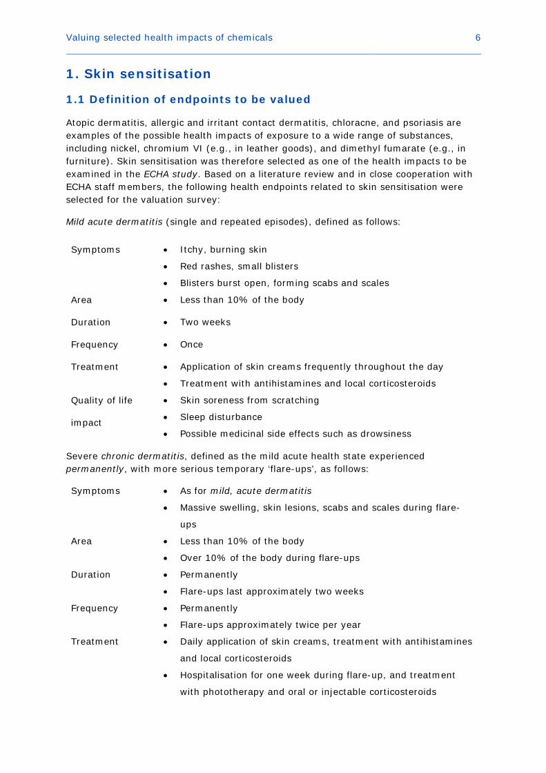
Atopic dermatitis, allergic and irritant contact dermatitis, chloracne, and psoriasis are examples of the possible health impacts of exposure to a wide range of substances, including nickel, chromium VI (e.g., in leather goods), and dimethyl fumarate (e.g., in furniture). Skin sensitisation was therefore selected as one of the health impacts to be examined in the ECHA study. Based on a literature review and in close cooperation with ECHA staff members, the following health endpoints related to skin sensitisation were selected for the valuation survey:
Mild acute dermatitis (single and repeated episodes), defined as follows:
Symptoms • Itchy, burning skin
• Red rashes, small blisters
• Blisters burst open, forming scabs and scales
Area • Less than 10% of the body
Duration • Two weeks
Frequency • Once
Treatment • Application of skin creams frequently throughout the day
• Treatment with antihistamines and local corticosteroids
Quality of life
impact
• Skin soreness from scratching
• Sleep disturbance
• Possible medicinal side effects such as drowsiness
Severe chronic dermatitis, defined as the mild acute health state experienced permanently, with more serious temporary ‘flare-ups’, as follows:
Symptoms • As for mild, acute dermatitis
• Massive swelling, skin lesions, scabs and scales during flare-
ups
Area • Less than 10% of the body
• Over 10% of the body during flare-ups
Duration • Permanently
• Flare-ups last approximately two weeks
Frequency • Permanently
• Flare-ups approximately twice per year
Treatment • Daily application of skin creams, treatment with antihistamines
and local corticosteroids
• Hospitalisation for one week during flare-up, and treatment
with phototherapy and oral or injectable corticosteroids
Valuing selected health impacts of chemicals 7
Quality of life
impact
• As for mild, acute dermatitis
• Inability to work in certain types of occupation during flare-
ups:
• Unpleasant and unsightly appearance
• Limits on leisure activities
Clearly, these are quite specific and narrowly-defined descriptions of endpoints which, in practice, are likely to vary in terms of their durations, severity and impacts. One issue is therefore the extent to which these descriptions match the illnesses which are likely to pertain in any particular context.
1.2 Description of the study and main results
The willingness to pay (WTP) to prevent the endpoints in question from occurring were elicited from an adult population sample in four EU Member States: the Czech Republic, Italy, the Netherlands and the United Kingdom using a combination of two stated- preference valuation approaches: contingent valuation (CV) and standard gambles (SG) with chaining.1 The resulting data were cleaned for ‘speeders’ (those who were judged to have completed the questionnaire unreasonably quickly, about 3.6% of respondents), ‘protesters’ (those who objected to the principle of providing a value (even zero) for avoiding the health episodes, around 10% of respondents) and outliers (those judged to have provided unreasonably high or low WTP responses). This data cleaning approach left just over 3,000 respondents. After adjusting for differences in purchasing power parity (PPP) across the EU, EU-wide benefit values were derived (Table 1).
The value of avoiding one case of mild, acute dermatitis was valued at around €2012 227. Various combinations of this illness were valued – for instance, avoidance of four such cases over a one-year period was valued at around €2012 329; the value of avoiding five episodes over a five-year period (one per year) was valued at around €2012 352, and the value of avoiding four episodes per year for 10 years (40 episodes in total) was valued at around €2012 615. The avoidance of a case of severe chronic dermatitis was valued at around €2012 1,055.
1.3 Evaluation of the results
A number of questions and observations are pertinent when evaluating these results. First, is the estimated WTP value for avoiding one case of acute dermatitis reasonable? At first sight, €2012 227 might be considered quite high – almost one per cent of per capita EU28 GDP of €26,400 in 2012 – for a condition with relatively mild symptoms and no significant impacts on everyday life2. There do not appear to be any existing estimates in the literature of the value of preventing acute dermatitis episodes, against which to compare. There are, however, estimates of the value of avoiding days with minor symptoms caused, e.g., by pollution episodes. Previous European estimates of the value of ‘symptom days’ have been around €2012 50 (Ready et al. 2004) and €2012 37 1 A two-way payment ladder corresponding to a double-bounded discrete-choice mechanism was employed for the elicitation of WTP in discrete intervals (Carson and Hanemann, 2005). 2 See http://ec.europa.eu/eurostat/tgm/table.do?tab=table&init=1&language=en&pcode=tec00001&plugin=1

Valuing selected health impacts of chemicals 8
(Maca et al. 2011).3 Given that the acute dermatitis episode in the ECHA study was defined as lasting for two weeks, the €2012 227 estimate is actually quite low compared with existing valuations of single symptom days.
Table 1: Willingness-to-pay values for skin irritation (scaled to EU28)
Health endpoint €2012 Mild, acute dermatitis 227
2x/year 289
4x/year 329
1x/year for 2 years 308
1x/year for 5 years 352
1x/year for 10 years 339
2x/year for 2 years 271
2x/year for 5 years 391
2x/year for 10 years 447
4x/year for 2 years 334
4x/year for 5 years 383
4x/year for 10 years 615
Severe, chronic dermatitis 1,055
Source: Maca et al. (2014)
However, the valuation of multiple occurrence of the endpoint over one or more years implies values per two-week episode much lower than €2012 227, questioning the scope sensitivity of these results. The value of preventing one episode per year for 10 years is only 50 per cent higher than the value of preventing a single episode, and actually lower than the value of preventing one episode per year for five years. These ‘multiple occurrence’ values imply annual discount rates of around 200 per cent, which are far in excess of what would be expected for private individuals in such a situation.4 The within-year (twice or four-times per year) values similarly exhibit extreme levels of ‘diminishing returns’, such that the second episode in the current year is valued at only €2012 62 (€2012
289 - €2012 227), and the third and fourth episodes are valued at only €2012 20 each 3 Ready et al. (2004) estimated values for a day of eye irritation (a ‘minor symptom day’), a day of coughing (a ‘minor restricted-activity day’) and a day of stomach upset (a ‘work-loss day’), all of which were valued approximately the same in utility-loss terms. Maca et al. (2011) estimated the value of a ‘cough day’. 4 Indeed, it is arguable whether respondents should report values for these multi-year combinations that demonstrate significant discounting or diminishing returns at all. The contingent scenario asked respondents to assume they could spread payments out across the time period in question, so no budget constraints should have been binding. Episodes were sufficiently infrequent to not ‘getting accustomed’ to the negative impacts, and in fact, if individuals expected their real incomes to grow over time, their valuations of health impacts should also grow. Finally, within a dynamic context, there appears no particular reason for why an illness experienced and valued in one year should be valued any differently from the same illness experienced and valued a year later.

Valuing selected health impacts of chemicals 9
((€2012 329 - €2012 289)/2).5 In the limit, the four times per year for 10 years result implies a per-episode value of €2012 15 (assuming no discounting) – an order of magnitude smaller than the valuation of a single (one-off) episode – or, alternatively, a discount rate of over 500 per cent.
These results seem to suggest that respondents’ valuations were insensitive to the scope of the health improvement on offer. T-tests indicate that the values expressed for different combinations are, at least, statistically significantly different from one another in general, which might be interpreted as ‘weak’ scope sensitivity (Maca et al. 2015). This might be of no great surprise since, as already stated, the value of just a single episode was estimated at almost one per cent of average annual income. So the same per episode valuation for the prevention of four episodes in a year would represent a large financial undertaking – individuals’ budget constraints (especially for discretionary but unplanned expenditure of the type considered in this survey) might be expected to bind quite soon at this range of values, even if the contingent scenario stated that payments could be made in instalments.
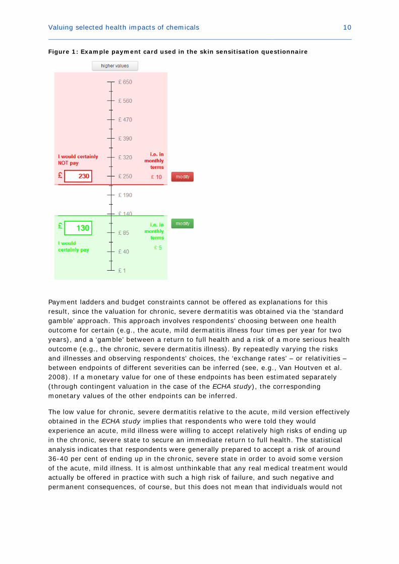
In addition, the payment instrument used in the questionnaire was a version of a ‘payment card’ with bids ranging from €1 (£1) up to €650 (£650), see Figure 1. Respondents were able to select higher values than €650 – as might be appropriate when valuing multiple (up to 40) episodes of an illness which they on average valued at €2012 227, but only by explicitly clicking on a button at the top of their screen. If respondents did not do this, they would have been presented with the same range of values for each multiple of the illness they were presented with (and without reference to the values they had expressed for other multiples of the same illness). This might have unintentionally encouraged respondents to select values from a restricted range, independent of the range of severity represented by the illness multiples they were asked to value.
Some of the multiple-episode scenarios could be said to describe chronic, albeit periodic, conditions, and in fact were included in the ECHA study so that the relationship between the valuation of acute and chronic illnesses could be examined. The explicitly chronic dermatitis condition specified in the study involved the symptoms of the acute condition permanently (rather than just for two weeks at a time) – or for around 40 years given the average age of the sample of about 41 – with, every six months or so, a two-week ‘flare-up’ which would be so bad as to necessitate a one-week stay in hospital. This would seem to be a much more severe disease than any of the multi-episode acute combinations, and yet the valuation obtained was (at €2012 1,055) only four times higher than the value of a single, two-week episode of mild dermatitis.
5 This implies an annual discount rate of almost 10,000 per cent.
Valuing selected health impacts of chemicals 10
Figure 1: Example payment card used in the skin sensitisation questionnaire
Payment ladders and budget constraints cannot be offered as explanations for this result, since the valuation for chronic, severe dermatitis was obtained via the ‘standard gamble’ approach. This approach involves respondents’ choosing between one health outcome for certain (e.g., the acute, mild dermatitis illness four times per year for two years), and a ‘gamble’ between a return to full health and a risk of a more serious health outcome (e.g., the chronic, severe dermatitis illness). By repeatedly varying the risks and illnesses and observing respondents’ choices, the ‘exchange rates’ – or relativities – between endpoints of different severities can be inferred (see, e.g., Van Houtven et al. 2008). If a monetary value for one of these endpoints has been estimated separately (through contingent valuation in the case of the ECHA study), the corresponding monetary values of the other endpoints can be inferred.
The low value for chronic, severe dermatitis relative to the acute, mild version effectively obtained in the ECHA study implies that respondents who were told they would experience an acute, mild illness were willing to accept relatively high risks of ending up in the chronic, severe state to secure an immediate return to full health. The statistical analysis indicates that respondents were generally prepared to accept a risk of around 36-40 per cent of ending up in the chronic, severe state in order to avoid some version of the acute, mild illness. It is almost unthinkable that any real medical treatment would actually be offered in practice with such a high risk of failure, and such negative and permanent consequences, of course, but this does not mean that individuals would not

Valuing selected health impacts of chemicals 11
be prepared to accept one.6 The analysis shows that respondents were willing to accept a higher risk of failure to avoid worse multiples of the mild illness, as might be hoped if individuals are to exhibit coherent preferences. However, the degree of variation in the accepted risk was not high compared with the apparent range of severity of the illness multiples – around 10 per cent variation in risk (36-40 per cent) compared with a five-fold (undiscounted) variation in severity (four episodes over two years to twenty episodes over 10 years). Similar to the contingent valuation results, this might be termed evidence of ‘weak’ scope sensitivity – respondents did vary the risks they said they would be prepared to accept, but not by as much as might perhaps be expected given how much the seriousness of the alternative varied.
The variation in risk in the standard gambles was even lower than the variation in WTP in the contingent valuation, which has already been suggested to be low – a 10 per cent variation in risk (36-40 per cent) compared with a 65 per cent difference between the WTP to avoid four episodes over two years (€2012 271) and the WTP to avoid 20 episodes over 10 years (€2012 447). One upshot of this ‘mismatch’ between the WTP and risk variation is that the resulting value for chronic, severe dermatitis depends on the WTP/risk estimate ‘exchange rates’ the value is inferred from – €2012 710 based on four acute episodes over two years, and €2012 1,482 on 20 episodes over 10 years.7 Moreover, the risks of the chronic, severe illness which respondents said they were prepared to accept were actually marginally lower for multiples of the mild, acute illness, which involved four episodes per year rather than two. Although the difference is not major (36.6 per cent risk to avoid two episodes per year for four years, compared with 36.8 per cent for two episodes for two years), this is further evidence that the standard gamble results for chronic, severe dermatitis, and the calculated monetary valuation, might not be very reliable.
In summary, the preceding discussion has suggested that the ECHA study produced a result for a single episode of acute, mild dermatitis, which – while high – seems to be accurate (even more so when compared with existing values for ‘symptom days’). However, in comparison, the values for multiple episodes of the same endpoint appear too low and insufficiently sensitive to variations in the number of episodes. The value for chronic, severe dermatitis appears much too low given that it is permanent and causes frequent and serious temporary ‘flair-ups’.
1.4 Evidence from the existing literature
The existing literature can be consulted for further evidence on the value of preventing skin sensitisation, and to provide ‘triangulation’ for the values obtained in the ECHA study. While no existing study appears to directly focusing on the valuation of avoiding skin sensitisation as result of chemicals exposure, several studies have been undertaken to estimate the quality of life effects of various skin conditions (e.g., atopic dermatitis, atopic eczema, psoriasis). Some of them also consider the utility and monetary valuation of impacts and treatments related to the evaluation of chronic dermatitis. No study was 6 The willingness to gamble when facing negative health outcomes is consistent with risk seeking behaviour in the loss domain as postulated by prospect theory (Kahneman and Tversky, 1992). 7 The value of €2012 1,055 proposed by Maca et al. (2014) for chronic, severe dermatitis (Table 1) is apparently based on the mean of the range of estimates obtained. The authors do acknowledge the weaknesses in the standard gamble results, however, and recommend that they be treated with caution.
Valuing selected health impacts of chemicals 12
found that considered only short-term, acute episodes (although chronic illnesses might have involved acute episodes). All studies found came from the health technology assessment and related literature, and not all of them are well documented (e.g., abstracts of unpublished conference papers) or undertaken to an academic standard equivalent to the ECHA study.
Of eight studies that considered the monetary valuation of the symptoms of psoriasis and dermatitis, two are of particular interest. The study by Lundberg et al. (1999) surveyed 336 psoriasis and eczema patients in Sweden. Responses to the Dermatology Life Quality Index (DLQI) suggested that conditions experienced were generally at the mild end of the severity spectrum (mean DLQI score 5.9 for psoriasis and 7.3 for eczema). Participants were asked how much they would be willing to pay for a new treatment that could on a monthly basis completely alleviate their symptoms with no side effects. Resulting values were €113-128 (uprated to 2012 prices) per month for eczema, and €147-228 per month for psoriasis, depending on the elicitation method used.
Hauber et al. (2011) surveyed 415 patients with (self-reported) mild-to-moderate psoriasis. They used a discrete choice experiment with attributes that describe the severity of psoriasis lesions after treatment and the percentage body surface area (BSA) affected. Different questions were asked for psoriasis said to affect the sufferer’s torso or their arms and legs. The results indicated that individuals were willing to pay more for a cure for psoriasis on their arms and legs than on their torso, more when their initial psoriasis was more severe, and more when a larger BSA was affected. More specifically, values (converted at PPP and uprated to 2012 prices) were estimated at €85 per month for the alleviation of mild severity lesions on the torso and covering five per cent BSA (€115 when on arms and legs), up to €450 per month for very severe lesions on the arms and legs and covering 25 per cent BSA (€399 torso). Thus, respondents valued very severe lesions over 25 per cent of the body around four to five-times worse than mild lesions over just five per cent of the body. Complete clearance of symptoms did receive a valuation premium, i.e. the improvement from mild to zero lesions was valued more than improvements from very severe to severe, severe to moderate, or moderate to mild.
A large number of studies have measured the impact of skin diseases and their treatments based on general quality of life metrics. Yang et al. (2014) review nine such studies which used the EQ5D life quality index to assess psoriasis impacts and treatment, with weights between 0.59 to 0.82. The study by Schmitt et al. (2008) is of particular interest for a number of reasons. First, it used descriptions of atopic eczema and psoriasis, which were quite similar to those used in the ECHA study. For instance, ‘controlled atopic eczema’ was said to affected less than 10 per cent of the patient’s body, involved mild itching but no sleep disturbance, and was effectively controlled by daily application of emollients. The ‘uncontrolled’ version was said to affect over 10 per cent of the patient’s body, with moderate-to-severe itching and occasional sleep disturbance; daily application of emollients was necessary but was not sufficient to prevent a flare-up once a year which would be bad enough to require hospitalisation. Both seem similar to, but slightly less severe than, the acute and chronic episodes in the ECHA study. Schmitt et al. (2008) surveyed patients suffering from atopic eczema and psoriasis as well as members of the general public, and elicited time-trade off (TTO) weights (Dolan et al. 1996; Dolan, 1997) and monthly WTP for a cure with no side

Valuing selected health impacts of chemicals 13
effects. Once sample characteristics were controlled for, no significant differences were found between median responses from each sub-sample.8 General population median TTO weights were 0.97 and 0.64 (controlled and uncontrolled atopic eczema, respectively) and 0.93 and 0.56 (controlled and uncontrolled psoriasis); median monthly WTP was €2012 54, €2012 163, €2012 82, and €2012 218 respectively for the four diseases. As in the ECHA study, the relative severities expressed in the TTO weightings did not translate into similar relativities in WTP.
An idea of how much disability assessments provided in some of the reviewed studies might mean in monetary terms can be obtained from applying the value of a life year metric (VOLY) to value the loss in QALYs.9 For example, the VOLY implied by the NewExt study (2003, p. III-34) amounts to about €64,000 (median) and €144,000 (mean) in 2012 prices.10 A disability weight of 0.97 (Lundberg et al. (1999), psoriasis, SG) is hence equal to €160 (€360) per month based on the median (mean) VOLY.11 A weight of 0.78 (Zug et al. (1995), psoriasis 10-30 per cent BSA, SG) implies a valuation of €1,176 (median) or €2,640 (mean) per month. Weights of 0.88 and 0.45 (Schmitt et al. (2008), controlled and uncontrolled psoriasis, TTO, based on responses from patients with psoriasis) result in median valuations of €641 and €2,940 per month for controlled and uncontrolled psoriasis respectively (€1,440 and €6,601 per month based on the mean VOLY). Except for the Lundberg et al. study, these benefit transfer values are substantially higher than those found in studies which have measured WTP directly. However, this is to be expected given that the VOLY is based on individuals’ preferences for reductions in mortality risk.
1.5 Recommended values for the prevention of skin sensitisation
The ECHA study appears to be by far the largest survey to date of individual WTP for preventing diseases associated with skin sensitisation. It was based on extensive piloting and design work, using state-of-the-art elicitation and estimation techniques, and the results exhibit some important features which support basic validity. This compares with existing skin disease valuation studies, which have generally been based on small sample sizes and unsophisticated valuation approaches. The ECHA study therefore represents an important contribution to the field.
The value for one acute episode of mild dermatitis lasting approximately two weeks, estimated in the ECHA study at €2012 227, matches quite well with previous WTP estimates of mild symptoms (e.g., Ready et al. 2004) and mild dermatitis (e.g., Lundberg et al. 1999), as well as with values based on monetised disability weights (Lundberg et al. 1999; Schmitt et al. 2008). On the other hand, the
8 Mean responses were not reported due to skewed distributions of the responses. The TTO weighting for uncontrolled atopic eczema reported by those with psoriasis was significantly lower than the weighting reported by the other two groups, even after controlling for sample differences, but this was the only such result. 9 It should be noted that this benefit transfer technique presumes the value of a QALY (or DALY) is a constant, which is hard to reconcile with the conceptual model of the VSL (Hammitt 2013). 10 Note that these figures are somewhat larger than the €2005 40,000 VOLY estimated in a recent nine-country European CV study (Desaigues et al. 2011), but consistent with the VOLY of €2012
200,000 that corresponds to the VSL estimates of Alberini and Ščasný (2014), see Section 5 for more details. 11 (1-0.97) × €64,000 ÷ 12 months = €160/month.
Valuing selected health impacts of chemicals 14
ECHA study’s value of preventing a case of severe, chronic dermatitis seems too low (at €2012 1,055), considering that it involves the mild version permanently and regular ‘flare-ups’ which are bad enough to require admission to hospital. There is no WTP or quality of life study which explicitly refers to this mild-severe illness profile. The Hauber et al. (2011) study valued a comparable mild skin disease at around €100 per month, and a comparable severe condition around €400 per month, which might imply a value for the health profile used in the ECHA study of around €1,800 per year (rather than €1,055 per case). A value based on the Schmitt et al. (2008) weights for controlled and uncontrolled psoriasis and the median VOLY of NewExt (2003) would approach €12,000 per year. Either of these benefit transfer values seems more reasonable for severe, chronic dermatitis.12
In between, there are the ECHA study values for multiple episodes of acute, mild dermatitis. These tend to be higher the more episodes are being valued (albeit not always), but often not all that much higher, so that the marginal value of additional episodes falls sharply. Although economic theory would generally predict declining marginal values (through, for example, discounting and diminishing returns), the rate of decline found in the ECHA study is extreme to the extent that implied discount rates range from around 200 per cent to almost 10,000 per cent per annum. The most obvious explanation would seem to be that the payment ladder used to elicit values (Figure 1) caused survey participants to anchor their responses within the range initially presented on the ladder, and that the resulting values for multiple episodes are therefore unreliable.13
Ultimately, which values to use depends on the relevant and available epidemiological endpoints and how they match with the health endpoints evaluated in the ECHA study. Multiple episodes of acute illnesses might be appropriate for air pollution, which varies randomly, but possibly not for the types of chemicals exposure which causes skin diseases. However, there could be some acute episodes associated with any exposure that cause chronic illnesses – either as ‘on-off’ illnesses for those exposed only occasionally or as distinct episodes experienced as part of the sensitisation process leading up to chronic illness. Whether the epidemiological functions used in any given impact assessment are sensitive enough to pick this type of variation up remains to be seen. The expectation is that most will be specified in terms of the prevalence of chronic disease, in which case per year values are most appropriate and useful.
12 These annual values could, of course, be converted into a cost per case by assuming an average age of onset and life expectancy for those affected, and applying an appropriate discount rate. 13 Navrud (2001) undertook a contingent valuation study of the avoidance of a range of air pollution-related acute respiratory illnesses each lasting one day. Half of his sample were asked to value one additional day of each illness over the following 12 months. The other half were asked to value 14 days over the same period. The cause of the illnesses, how they would be avoided, and how their avoidance would be paid for were not specified in the questionnaire. Navrud (2001) found that the mean per day values for the second ‘14 day’ sample were between one third and one fifth of the per day values for the first ‘single day’ sample, and declared the results ‘as expected from economic theory, and in general […] reasonable with regard to the seriousness of the different symptoms’ (p. 315) – although he provided no other evidence to substantiate this. He did not account for possible discounting of episode values over the 12 month period.

Valuing selected health impacts of chemicals 15
2. Kidney failure and kidney disease
2.1 Definition of endpoints to be valued
The kidneys perform the vital function of biotransforming toxicants and eliminating them through the excretion of metabolic waste, thereby maintaining human health. The kidneys can be seriously affected by exposure to heavy metals, as well as certain organic solvents and polycyclic aromatic hydrocarbons (PAHs). The U.S. EPA (2000a) identified nine contaminants of concern because of their link to kidney disease: cadmium, pentachlorophenol, methylene chloride, toluene, pyrene, fluoranthene, ethylbenzene, nitrobenzene, and pentachlorobenzene. Kidney disease and kidney failure were therefore selected as one of the health impacts to be examined in the ECHA study. Based on a literature review and in close cooperation with ECHA staff members, the following health outcomes related to kidney failure were selected for the valuation study:
Acute kidney injury, defined as follows:
Symptoms • Impaired urine production
• Nausea and vomiting, reduced appetite
• Shortness of breath, bad breath
• Weight loss or gain
• Itching, dry skin
• Fatigue, sleep disturbance
Duration • Four weeks: two weeks in hospital, two weeks recovery at
home
Frequency • Once
Treatment • Two-week hospitalisation for dialysis treatment to improve
kidney function
Quality of life
impact
• Permanent dietary changes required
• No symptoms or daily limitations after four weeks
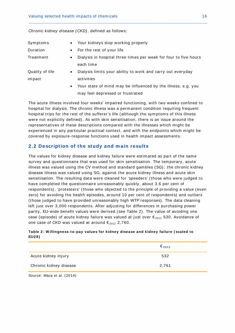
Valuing selected health impacts of chemicals 16
Chronic kidney disease (CKD), defined as follows:
Symptoms • Your kidneys stop working properly
Duration • For the rest of your life
Treatment • Dialysis in hospital three times per week for four to five hours
each time
Quality of life
impact
• Dialysis limits your ability to work and carry out everyday
activities
• Your state of mind may be influenced by the illness, e.g. you
may feel depressed or frustrated
The acute illness involved four weeks’ impaired functioning, with two weeks confined to hospital for dialysis. The chronic illness was a permanent condition requiring frequent hospital trips for the rest of the sufferer’s life (although the symptoms of this illness were not explicitly defined). As with skin sensitisation, there is an issue around the representatives of these descriptions compared with the illnesses which might be experienced in any particular practical context, and with the endpoints which might be covered by exposure-response functions used in health impact assessments.
2.2 Description of the study and main results
The values for kidney disease and kidney failure were estimated as part of the same survey and questionnaire that was used for skin sensitisation. The temporary, acute illness was valued using the CV method and standard gambles (SG); the chronic kidney disease illness was valued using SG, against the acute kidney illness and acute skin sensitisation. The resulting data were cleaned for ‘speeders’ (those who were judged to have completed the questionnaire unreasonably quickly, about 3.6 per cent of respondents), ‘protesters’ (those who objected to the principle of providing a value (even zero) for avoiding the health episodes, around 10 per cent of respondents) and outliers (those judged to have provided unreasonably high WTP responses). The data cleaning left just over 3,000 respondents. After adjusting for differences in purchasing power parity, EU-wide benefit values were derived (see Table 2). The value of avoiding one case (episode) of acute kidney failure was valued at just over €2012 530. Avoidance of one case of CKD was valued at around €2012 2,760.
Table 2: Willingness-to-pay values for kidney disease and kidney failure (scaled to EU28)
€2012
Acute kidney injury 532
Chronic kidney disease 2,761
Source: Maca et al. (2014)

Valuing selected health impacts of chemicals 17
2.3 Evaluation of the results
A number of observations can be made about these results. First, the estimated WTP value for avoiding one case of acute kidney failure seems relatively low compared with existing valuations of other mild morbidity symptoms. The illness was defined as lasting four weeks, with two of those weeks spent receiving treatment in hospital. However, as previously discussed, the value of preventing an episode of acute mild dermatitis – lasting only two weeks with no need for any significant treatment or hospital stays – was estimated to be only just under half the figure for acute kidney failure. The value of avoiding a hospital stay with air pollution-related respiratory symptoms was estimated in the Ready et al. (2004) study at a comparable €2012 462, despite being associated with only three days in hospital, instead of two weeks, and only five days’ – not 14 – recovery at home.
Similarly, the value of avoiding CKD, requiring four-hour hospital visits three times a week for the rest of a person’s life, was valued at an apparently low €2012 2,761. For comparison, the Ready et al. (2004) study valued a (reasonably comparable) emergency room visit with respiratory symptoms at €2012 238. This might be said to imply that a course of hospital dialysis treatment lasting for only four weeks (around 12 visits) would have a similar cost as a course of treatment lasting 30 years at this hospital visit unit value.
As with the dermatitis results discussed earlier, these figures indicate a lack of discrimination between acute and chronic health states in terms of their severity. This difference in severity was also measured in terms of health utility losses estimated via a visual analogue scale exercise in the questionnaire. The derived QALY losses correspond to 0.028 and 0.558, respectively, meaning that respondents judged the chronic condition almost twenty times worse than the acute episode. Thus, as before, it would appear that respondents were unable or unwilling to translate this assessed difference in physical severity into a commensurate difference in WTP. If the QALY loss estimates were translated into WTP values using the aforementioned €2012 64,163 NewExt VOLY, the resulting values would be €1,796 for the acute episode – more than three times the value estimated via the WTP questions – and €35,803 per year for the chronic illness – over ten times higher than the WTP value obtained from the questionnaire for the permanent condition.
2.4 Evidence from the existing literature
Few studies were identified which have attempted to measure WTP for health outcomes associated with kidney failure. Herold (2010) estimated the WTP of patients suffering from end-stage renal disease (ESRD) for a kidney so they could have a transplant. 107 US patients with ESRD completed a rather rudimentary self-administered internet-based survey. 78.5 per cent said they would be willing to pay for a kidney – although mean WTP is not reported, it can be estimated at around $10,000, or €2012 8,080 at purchasing power parity.14 The only other study identified was by Kjær et al. (2012), who examined
14 Proportions of the sample reporting WTP figures in a range of value bands are presented in Table 2 of Herold (2010). After accounting for the proportion who were unwilling to pay anything, taking the midpoints from the monetary intervals as approximate estimates of WTP, and assuming that those who reported WTP greater than $50,000 were actually only prepared to pay that amount (which underestimates their true WTP), a figure just below $10,000 is obtained. This could
Valuing selected health impacts of chemicals 18
preferences for establishing nephrology facilities in Greenland, but did not estimate valuations for prevention of the disease or reductions in its severity.
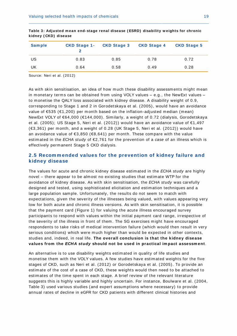
In comparison, there are a large number of studies which have estimated the impact of kidney disease on quality of life. Morimoto and Fukui (2002) undertook a comprehensive review of the literature up to the year 2000, and found 72 disability weights relating to ESRD – mean (weighted by sample size) weights were 0.522 (SG) and 0.566 (TTO) for haemodialysis, 0.51 (SG) and 0.514 (TTO) for continuous ambulatory peritoneal dialysis and 0.565 (SG) and 0.721 (TTO) for transplant. There have been fewer studies since then, and few have considered the quality of life impact of other stages of kidney disease. Gorodetskaya et al. (2005) estimated TTO disability weights via a survey of 205 patients with CKD. Patients with Stage 1 and 2 disease reported a mean weight of 0.9, Stage 3 reported mean weight of 0.87, Stage 4 reported 0.85, and Stage 5 reported 0.77 (0.72 for those on dialysis).15 However, sample sizes within groups were small and means were not statistically significantly different (at the five per cent significance level) from each other.
Neri et al. (2012) estimated EQ5D disability weights from a survey of 181 UK and US patients who had received a kidney transplant. Results are reported in Table 3. Neri et al. (2012) found that UK participants consistently evaluated their health to be worse than their US counterparts, with Stage 5 kidney disease being clearly worse than other stages, as found by Gorodetskaya et al. (2005). Salomon et al. (2012) estimated disability weights as part of the Global Burden of Disease (GBD) 2010 update, as follows: Stage 4 CKD, 0.105; ESRD with transplant, 0.027; and, ESRD with dialysis, 0.573.16 The apparently low assessment of the impact of ESRD with a transplant on quality of life, compared with the other literature reviewed above, might well be explained by the description of this illness used in the GBD (“sometimes feels tired and down, and has some difficulty with daily activities,” Salomon et al. (2012, Appendix Table A 2), which does sound relatively minor compared with the description for ESRD with dialysis (“is tired and has itching, cramps, headache, joint pains and shortness of breath. The person needs intensive medical care every other day lasting about half a day”). The transplant description could be at odds with experience of patients in practice, especially as those who have received a transplant might still exhibit symptoms of CKD (Neri et al. 2012).
be an underestimate given that some zero responses are likely to be protests (individuals who have a positive value but reject the premise of the valuation exercise). 15 According to the Renal Association (www.renal.org), Stage 1 CKD is where kidney function is normal (as measured by an estimated Glomerular Filtration Rate (eGFR) of 90mls/min/1.73m2 or higher) but there is other evidence of kidney disease; Stage 2 CKD is mildly reduced kidney function (eGFR 60-89mls/min/1.73m2); In Stage 3 CKD, eGFR is approximately 30-60 per cent (eGFR 30-59mls/min/1.73m2); Stage 4 CKD is severely reduced kidney function (eGFR 15-29ml/min/1.73m2) and Stage 5 CKD is very severely reduced kidney function or ESRD (eGFR 15ml/min/1.73m2 or less). 16 Note that the GBD uses disability-adjusted life years (DALYs), which are measured from 0 (perfect health) to 1 (death), compared with QALYs, which are measured in the opposite direction.
Valuing selected health impacts of chemicals 19
Table 3: Adjusted mean end-stage renal disease (ESRD) disability weights for chronic kidney (CKD) disease
Sample CKD Stage 1-2
CKD Stage 3 CKD Stage 4 CKD Stage 5
US 0.83 0.85 0.78 0.72
UK 0.64 0.58 0.49 0.28
Source: Neri et al. (2012)
As with skin sensitisation, an idea of how much these disability assessments might mean in monetary terms can be obtained from using VOLY values – e.g., the NewExt values – to monetise the QALY loss associated with kidney disease. A disability weight of 0.9, corresponding to Stage 1 and 2 in Gorodetskaya et al. (2005), would have an avoidance value of €535 (€1,200) per month based on the inflation-adjusted median (mean) NewExt VOLY of €64,000 (€144,000). Similarly, a weight of 0.72 (dialysis, Gorodetskaya et al. (2005); US Stage 5, Neri et al. (2012)) would have an avoidance value of €1,497 (€3,361) per month, and a weight of 0.28 (UK Stage 5, Neri et al. (2012)) would have an avoidance value of €3,850 (€8,641) per month. These compare with the value estimated in the ECHA study of €2,761 for the prevention of a case of an illness which is effectively permanent Stage 5 CKD dialysis.
2.5 Recommended values for the prevention of kidney failure and kidney disease
The values for acute and chronic kidney disease estimated in the ECHA study are highly novel – there appear to be almost no existing studies that estimate WTP for the avoidance of kidney disease. As with skin sensitisation, the ECHA study was carefully designed and tested, using sophisticated elicitation and estimation techniques and a large population sample. Unfortunately, the results do not seem to match with expectations, given the severity of the illnesses being valued, with values appearing very low for both acute and chronic illness versions. As with skin sensitisation, it is possible that the payment card (Figure 1) for valuing the acute illness encouraged survey participants to respond with values within the initial payment card range, irrespective of the severity of the illness in front of them. The SG exercises might have encouraged respondents to take risks of medical intervention failure (which would then result in very serious conditions) which were much higher than would be expected in other contexts, studies and, indeed, in real life. The overall conclusion is that the kidney disease values from the ECHA study should not be used in practical impact assessment.
An alternative is to use disability weights estimated in quality of life studies and monetise them with the VOLY values. A few studies have estimated weights for the five stages of CKD, such as Neri et al. (2012) or Gorodetskaya et al. (2005). To provide an estimate of the cost of a case of CKD, these weights would then need to be attached to estimates of the time spent in each stage. A brief review of the relevant literature suggests this is highly variable and highly uncertain. For instance, Boulware et al. (2004, Table 3) used various studies (and expert assumptions where necessary) to provide annual rates of decline in eGFR for CKD patients with different clinical histories and
Valuing selected health impacts of chemicals 20
proteinuria status.17 These would imply an individual might take 20 years to progress from Stage 1 to Stage 4, with a progression to Stage 5 taking another four or five years. Blanchette et al. (2015) examined a database of almost 30,000 CKD patients over a limited follow-up period. They found median transition times between only five and eight months, and a very small number of patients transitioned from Stage 1 to Stage 5 in only two months. However, over half of patients did not transition at all over the follow-up period, and almost a quarter actually went back a stage. Although the short follow-up time might limit the applicability of the Blanchette et al. (2015) results to the estimation of mean disease duration, they illustrate how variable and how quick disease progression can be.
There is also the question of the impact on life expectancy of contracting CKD. This will depend on the individual’s age at the time the disease is contracted, how rapid the progression is and what sort of treatment is received. The Boulware et al. (2004) analysis suggests a mean progression of around 20-25 years from Stage 1 to Stage 5. According to the US National Kidney Foundation, patients on dialysis have a life expectancy of 5-10 years (although this can vary significantly), if they do not receive a transplant.18 This might imply a total disease duration of, say, 33 years, which in turn could suggest a reduction in life expectancy for a 40-year old of around nine years.19 Using a discount rate of four per cent, this would give a value of just under €310,000, using the Gorodetskaya et al. (2005) disability weights and the median NewExt VOLY. Using the mean of the Neri et al. (2012) weights in Table 3 would give a figure almost 70 per cent higher than this. On top of this would need to be added the costs of treatment, which can be considerable, especially for ESRD.20
This is just an illustration of the way in which a value for preventing CKD could be constructed using disability weights and other relevant information. It also serves to demonstrate the potential magnitude of the values which could be obtained (as well as underlining just how low the result obtained from the ECHA study are compared to other evidence). As was the case with skin sensitisation, the available toxicological and epidemiological evidence will help to determine what value should be constructed in any particular case. For instance, CKD caused by chemicals exposure might be associated with more rapid progression than suggested by Boulware et al. (2004), which could increase the costs by bringing forward the more severe Stage 5 CKD and possibly shortening life expectancy even further. It is outside the scope of this review to explore these issues in detail.
17 Protein in the urine is a common sign of kidney damage. 18 https://www.kidney.org/atoz/content/dialysisinfo 19 Based on a life expectancy at 40 of just under 42 years for the Euro 28 in 2013 (Eurostat database table demo_mlexpec at www. eurostat.ec.europa.eu). 20 For instance, Kerr et al. (2012) estimated a mean annual financial cost to the UK health service of dialysis treatment of £23,426 in 2010. They also estimated that CKD was associated with excess risk of stroke and heart attack.
Valuing selected health impacts of chemicals 21
3. Fertility and developmental toxicity
3.1 Definition of endpoints to be valued
Exposure to certain chemicals can increase the risk of reduced fertility due to several reproductive dysfunctions, including lower sperm count, lower sperm motility, changes in the oestrogen cycle, changes in hormone levels, changes in sexual behaviour, and spontaneous abortion (Kumar and Burton 2008). In addition, maternal exposure to pesticides, polychlorinated biphenyls (PCBs), polychlorinated dibenzofurans (PCDFs), lead, mercury, and other endocrine disruptors might lead to various birth defects (Wigle et al. 2008). A summary by the U.S. EPA (2013) found that environmental contaminants (e.g., lead, methylmercury, PCBs, cadmium, arsenic, and manganese) can damage a child’s developing brain and nervous system and cause neuro-developmental effects such as learning difficulties, reduced cognitive development, lowered intelligence and behavioural problems such as attention deficit and impulsive behaviour.
For these reasons, fertility and developmental toxicity were selected as a set of health impacts to be examined in the ECHA study. Based on a literature review and in close cooperation with ECHA staff members, the following broad health outcomes related to fertility and developmental toxicity were selected for the valuation survey:
• Probability of conception
• Chance of successful in vitro fertilisation (IVF)
• Risk of minor birth defects
• Risk of congenital disorders and birth defects to the internal organs
• Risk of major external birth defects
• Risk of very low birth weight (VLBW) with associated risk of future developmental
problems
Each of these broad health outcomes has a range of specific impacts on wellbeing and quality of life, for parents, the individual affected (e.g., an infertile woman or an unborn child), or the ‘general public’. In most (if not all) cases, the actual outcomes associated with a specific instance of, for instance, VLBW cannot be known in advance. As a result, survey participants were presented with general descriptions of symptoms, impacts, and risks associated with a particular health outcome ‘class’, as contextual information on which to base their responses to subsequent valuation questions. (See Ščasný and Zvěřinová (2014) for more details and actual descriptions and information provided to respondents.)
Two different populations were sampled: those who intended to have children in future; and the general population (some of whom might intend to have children in future). Risks of the different outcomes were presented to potential parents and tailored to the age and sex of themselves and their partner. Other respondents were simply presented with EU average probabilities. Respondents were not told of the relative probabilities of different outcomes within the ‘basket’ of, for instance, ‘minor birth defects’ since these data are not readily available and, in any case, parents would generally not have access to such detailed information when making the sorts of choices involved in this situation.
Valuing selected health impacts of chemicals 22
3.2 Description of the study and main results
WTP values were elicited from samples of potential future parents and the general adult population in four EU Member States: the Czech Republic, the United Kingdom, the Netherlands and Italy. In total, 3,913 respondents were interviewed, and after cleaning the dataset (i.e., removing protest and ‘speeder’ (unfeasibly quick) responses) and allocating the respondents to the two samples, the datasets consisted of 1,363 valid interviews in the general population sample (some of whom were intended future parents but were recruited through the general population sample frame) and 2,625 valid interviews in the sample of intended future parents (all respondents who would like to have children in the future). There is therefore overlap between the two samples, and the latter sample includes respondents from the sample of the general population who intend to have children in future. Respondents were offered:
• a ‘private good’ in the form of a hypothetical vitamin complex, at a given cost, which would afford them a specified increase in conception probability or risk of developmental problems over a certain period of time; or,
• a ‘public good’ in the form of a package of stricter regulations on chemicals in products which afford similar improvements but across the whole EU population and at the cost of generalised increases in product prices.
Those who intended to have children in future were offered both private and public good version of the improvements. They were asked directly for their WTP to increase the probability of success if they were to have IFV treatment. Those who did not intend to have children in future were only offered the public good version of the improvements, and were not asked to value changes in the probability of success of IVF.
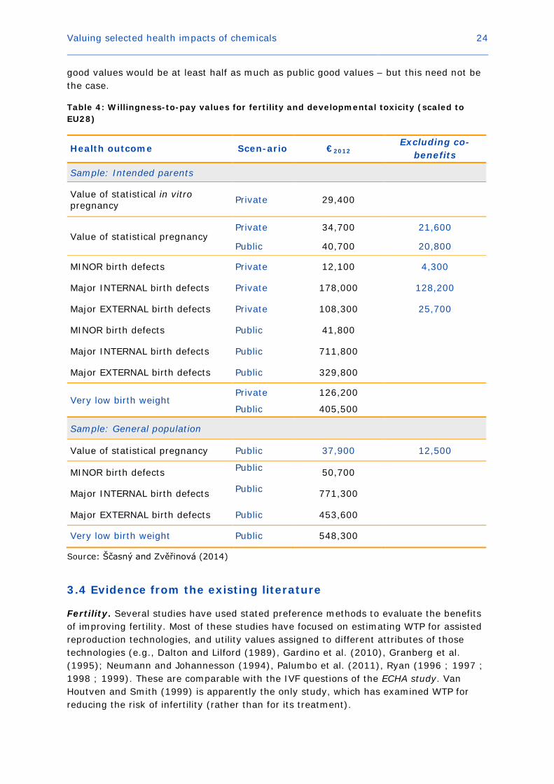
Table 4 provides EU-wide benefit estimates for each health outcome derived from two different populations and within two different valuation contexts (i.e., the private and public good scenario). These EU-wide numbers are computed from the population-weighted WTP values transferred to each EU Member State based on PPP adjustments and an income elasticity of WTP of 0.7. There are also additional estimates, which control for whether respondent said they assumed that additional benefits (‘co-benefits’) would be associated with taking the hypothetical vitamins or with the hypothetical reduction in chemicals in products. The numbers in bold are those recommended by Ščasný and Zvěřinová (2014) for use in REACH SEA.
The results suggest a value of statistical IVF pregnancy of €2012 29,400; the values for a natural conception (scaled up from a reduction in the probability of infertility) range from €2012 12,500 to €2012 40,700, depending on whether the good is public or private and whether or not co-benefits are included (see next section). The prevention of a case of VLBW was valued at €2012 126,200 from a private perspective, and at around €2012 0.4m-0.5m from a public perspective. Preventing a case of minor birth defects was valued as low as €2012 4,300 (private perspective, no co-benefits) and up to €2012 50,700 (general public perspective). Finally, major birth defects were costed at up to €2012 771,300 (internal defects from a general public perspective), and as low as €2012 25,700 (external defects from a private perspective with no co-benefits). Note that Ščasný and Zvěřinová (2014) caution against comparing the private and public good values because of differences in the way they were described, how the contingent market was set up, and how the values were elicited. However, although these factors might well affect the values which are reported by respondents, they do not in themselves relate to the
Valuing selected health impacts of chemicals 23
impacts of the health conditions in question, and hence there is no reason in principle why the public and private good values are not comparable.
3.3 Evaluation of the results
A number of observations can be made about these results. First, the ECHA study has made a significant contribution to the literature on the valuation of infertility and developmental toxicity, as this is an underexplored area with few comparable previous studies. For this reason, there is little existing evidence on which to make any firm evaluation of the ECHA study results. The values are therefore necessarily uncertain, but also potentially very important.
It is of some concern that the values for several endpoints seem to have been inflated by what Ščasný and Zvěřinová (2014) have termed ‘co-benefits’. Essentially, respondents who reported assuming that there would be other benefits associated with taking the hypothetical complex of vitamins – which was the vehicle for the private good risk reductions in the study – appear to have reported significantly higher WTP than those who reported that they took account only of the benefits actually described in the survey. In some cases, the ‘co-benefits’ actually account for the major portion of the total benefits of the risk reduction – for instance, the private value for preventing a statistical case of minor birth defects is estimated at €2012 12,100, but only €2012 4,300 if the co-benefits are stripped out, even though no such benefits were mentioned anywhere in the survey. This does not imply that these respondents actually did consider additional benefits when deciding upon their WTP; only that their WTP was systematically higher. While it is of concern that such respondents were able to influence the sample mean values to such a significant extent, it might simply reflect the fact that there exists varying views about what vitamin treatment can and cannot achieve.
As already noted, Ščasný and Zvěřinová (2014) advise against comparing the estimated private and public good values because of the different ways in which they were generated. This could be seen as an overly cautious position. Certainly, one would expect public good values to exceed private good values, had they been estimated based on answers of the same individuals (since they could expect to enjoy both types of value; i.e., the private benefits of risk reduction, as well as any ‘social’ or ‘external’ benefits of that risk reduction). This is what is observed in Table 4. However, one would not expect the public good values of those who would not benefit from private benefits (those who did not plan to have a child) to exceed the public good values of those who would.21 Yet this is what was found in the ECHA study for all birth defects. The only interpretation that comes to mind is that the different framing of the questions led respondents to express different preferences.
Finally, the public good values exceed the private good values significantly, even for the group of intended parents who valued both. However, there is no information on which to make a judgement about what sort of difference might be expected between the two. It seems likely to assume that health benefits for the individual(s) affected would be expected to exceed the benefits to society of the same health impacts – so that private
21 Recall that the general population sample included some individuals who were planning to have a child in the future, and who would therefore benefit personally from the public policy to reduce fertility and developmental risks from chemicals.
Valuing selected health impacts of chemicals 24
good values would be at least half as much as public good values – but this need not be the case.
Table 4: Willingness-to-pay values for fertility and developmental toxicity (scaled to EU28)
Health outcome Scen-ario €2012 Excluding co-
benefits
Sample: Intended parents
Value of statistical in vitro pregnancy Private 29,400
Value of statistical pregnancy Private 34,700 21,600
Public 40,700 20,800
MINOR birth defects Private 12,100 4,300
Major INTERNAL birth defects Private 178,000 128,200
Major EXTERNAL birth defects Private 108,300 25,700
MINOR birth defects Public 41,800
Major INTERNAL birth defects Public 711,800
Major EXTERNAL birth defects Public 329,800
Very low birth weight Private 126,200
Public 405,500
Sample: General population
Value of statistical pregnancy Public 37,900 12,500
MINOR birth defects Public 50,700
Major INTERNAL birth defects Public 771,300
Major EXTERNAL birth defects Public 453,600
Very low birth weight Public 548,300
Source: Ščasný and Zvěřinová (2014)
3.4 Evidence from the existing literature
Fertility. Several studies have used stated preference methods to evaluate the benefits of improving fertility. Most of these studies have focused on estimating WTP for assisted reproduction technologies, and utility values assigned to different attributes of those technologies (e.g., Dalton and Lilford (1989), Gardino et al. (2010), Granberg et al. (1995); Neumann and Johannesson (1994), Palumbo et al. (2011), Ryan (1996 ; 1997 ; 1998 ; 1999). These are comparable with the IVF questions of the ECHA study. Van Houtven and Smith (1999) is apparently the only study, which has examined WTP for reducing the risk of infertility (rather than for its treatment).

Valuing selected health impacts of chemicals 25
Both Neumann and Johannesson (1994) and van Houtven and Smith (1999) calculated the implied marginal WTP per ‘statistical baby’. In the former study, values for IVF treatment, assuming the respondent knew they were infertile, ranged from €2012 47,000 to €2012 204,000, with the higher figure for a 10 per cent chance of success and the higher figure for a 100 per cent success rate. The values for paying into an insurance scheme which would give access to IVF treatment if it were needed ranged from €2012
250,000 for a 100 per cent probability of success up to €2012 2m for a 10 per cent probability. The higher values for ex ante pregnancy are to be expected given diminishing marginal utility of income (although this would be tempered by the uncertainty about whether the treatment would be needed at all), but the higher values for lower probabilities are not.
This result might stem from the fact that WTP did not increase in proportion to the probability of success, which, the authors suggested, could reflect respondents’ anchoring their values for different probability levels on their first answer (for the lowest probability). Alternatively, there might be a reflection of respondents’ valuing the chance of IVF independent of the probability of success (although this does not seem a likely explanation for the ex post case when individuals were able to value the certainty of a successful course of IVF treatment, which must be more valuable to a couple hoping to get pregnant than a course of treatment which might fail). Finally, values for a public programme which would provide IVF treatment to couples who needed it, ranged from €2012 129,000 to €2012 1.13m, i.e. actually lower than the values for the private insurance scheme, even though in principle it would provide the same benefits for the respondent as well as any altruistic value they might attach to other couples being able to access treatment. The explanation suggested for this result was that respondents might have had doubts about the quality of care provided by a public programme, or simply objected to such a programme financed out of higher taxes.
The study by van Houtven and Smith (1999) was apparently the first to focus on individuals’ WTP for reductions in their own risk of infertility – through the purchase of a hypothetical medication which they could take at some time in the future (or not at all), and which would delay the natural reduction in fertility which comes with ageing. Therefore, estimates of WTP for reductions in infertility risks required an assumption about respondents’ discount rates and an estimate of when they would expect to start taking the drug. Of 188 respondents, 105 said they would not take the drug at the monthly price it was offered to them; 37 said they would take it within the next year, with only seven saying they would wait four or more years. Van Houtven and Smith calculated implied values of a statistical pregnancy from €2012 6,820 to €2012 51,830 (depending on the duration of the treatment). This was on the basis of assumed discount rates of three or five per cent, which might be considered low for private individuals, and higher discount rates would reduce these figures.22 Clearly, however, the values are orders of magnitude lower than those estimated by Neumann and Johannesson (1994).
22 Discount rates proposed for use in societal cost-benefit analysis (e.g. four per cent for the European Commission, 3.5 per cent for UK central government) tend to be influenced by societal factors, such as the ability to pool risk and concern for future generations, and as a result are expected to be lower than those calculated from the perspective of private households or firms. Empirical evidence on discount rates relating specifically to health impacts (as summarised by, for instance, Hammitt and Haninger (2010)) does not necessarily suggest values much different from these societal rates, however.
Valuing selected health impacts of chemicals 26
There have been relatively few studies of the impact of infertility on quality of life. Recent NICE (2013) guidance on the management of infertility used a study by Scotland et al. (2011), which had calculated a loss of 1.59 QALYs (discounted) from infertility for a woman with a remaining life expectancy of 56 years. This in turn was based on a disability weight of 0.82 estimated by Stratton et al. (2001), using the Health Utilities Index 2 (Torrance et al. 1996).23 This translates into a per-case value of €2012 102,000 at the NewExt median VOLY (uprated to 2012). Salomon et al. (2012) and Haagsma et al. (2015) both used the GBD 2010 instrument to estimate DALY weights for primary and secondary infertility of 0.011 and 0.006 (Salomon et al. 2012) and 0.008 and 0.007 (Haagsma et al. 2015). Using the same approach as Scotland et al. (2011), these weights would imply values per case from €2012 8,700 to €2012 16,000. Clearly, the GBD-based disability weights are much lower than the weight based on the Health Utilities Index 2. This could be related to the fact that the GBD health state descriptions for infertility make no mention of any physical or mental health symptoms associated with infertility, and the described conditions appear largely unproblematic.24
Developmental toxicity. A literature search suggested that no previous study has estimated the value of preventing birth defects or the effects of VLBW. Several economic studies considering developmental end-points have utilised the cost-of-illness method (e.g., Hutchings and Rushton, 2007; Olesen et al. 2012; Case and Canfield, 2009), but this approach does not cover (direct) impacts on individual wellbeing. Only a very small number of studies have estimated WTP for developmental health risk reductions, but those using production function approaches (Joyce et al. 1989; Agee and Crocker, 1996; Nastis and Crocker, 2003; 2012) have not done so in a way which permits calculation of the value of preventing (statistical) cases of specific – or baskets of – health outcomes. Von Stackelberg and Hammitt (2009) administered stated preference surveys in the context of environmental and developmental impacts of exposure to PCBs, but focussed specifically on two narrow health endpoints – IQ and reading comprehension. As such, although these two endpoints might be components of the overall health outcomes associated with VLBW and some birth defects, their work is also not closely comparable with the ECHA study.
In comparison, there has been a considerable amount of effort to estimate the impacts on quality of life of specific birth defects and of VLBW generally. For instance, Van den Akker-van Marle et al. (2013) reported an estimate of 0.84 undiscounted QALYs lost per case of cryptorchidism, but based on a survey of only 41 respondents and visual analogue scale (VAS) results ‘transformed’ to TTO. This would translate into a discounted value of 0.25 QALYs per case, assuming an 80-year life expectancy at birth and a four per cent discount rate – which in turn implies a value per case of just over €16,000 per case at the uprated NewExt median VOLY. Jentink et al. (2012) estimated a very similar 0.8 QALYs (undiscounted) per case of hypospadias, although Olsson et al. (2014), citing Schönbucher et al.’s (2008) review, suggest that medical treatment of this condition has improved and that therefore the Jentink et al. (2012) assessment might be too high.
23 The disability weight for ‘normal health’ in the Health Utilities Index 2 is 0.89, giving a decrement associated with each year of infertility of 0.07 QALYs. 24 Primary infertility in the GBD 2010 is described as, ‘wants to have a child and has a fertile partner, but the couple cannot conceive’, while secondary infertility is described as, ‘has at least one child, and wants to have more children. The person has a fertile partner, but the couple cannot conceive.’
Valuing selected health impacts of chemicals 27
Wehby et al. (2006) used a VAS in a survey of 330 medical professionals to estimate disability weights for various types of oral clefts. These ranged from 0.64-0.95, depending on the type of cleft and age of the patient. The value per case would depend on how long the patient experienced the effects and how successful was the treatment.
However, these studies looking at specific birth defects can only provide contextual information for the ECHA study, which considered ‘birth defects’ as a basket of possible conditions of varying unspecified probabilities. Thus, the values are only meaningfully comparable to those estimated in the ECHA study, if they were aggregated and weighted by the probability of occurrence. It is beyond the scope of this report to undertake this exercise.
Two very interesting studies consider the impact of VLBW on subsequent quality of life. Rautava et al. (2009) undertook a national study of all VLBW infants born in Finland between 2000 and 2003. 1,169 (900 live-born) children were compared against 368 full-term controls. Compared with the controls, 1.3 QALYs had been lost by each VLBW by age 5. This implies a discounted cost per case of around €75,000 based on the NewExt median VOLY. Given that VLBW is likely to result in negative health implications throughout the individual’s life, the total cost would likely be higher than this figure. Similarly, Petrou et al. (2009) surveyed 190 ‘extremely preterm’ children at age 11 and compared them with 141 full-term classmates. ‘Extremely preterm’ was defined as being born before the end of the 25th week of gestation, and was suggested to be a comparable, but more up-to-date definition of VLBW. Using the Health Utilities Index 3 (Feeny et al. 2002), they estimated a mean decrement in quality of life of 0.167 QALYs for the children who had been born extremely preterm. If we assume this decrement had persisted throughout the child’s life up until that point, this would imply a discounted cost per case of €94,000 at the NewExt median.

Valuing selected health impacts of chemicals 28
3.5 Recommended values for the prevention of fertility and developmental toxicity
The ECHA study on developmental toxicity represents a significant contribution to an extremely sparse literature. It used ‘realistic’ endpoints that reflect the inherent uncertainty over actual outcomes associated with these types of effects. It provided comprehensive and realistic information on risks and possible health impacts, within the context of realistic policy scenarios. As with other surveys, elicitation and estimation techniques were ‘state of the art.’
The study’s novelty does, of course, mean that there are few comparable studies against which to evaluate the results, especially for VLBW and birth defects. Regarding the value of fertility, the study by van Houtven and Smith (1999) would seem to have provided the inspiration for the ECHA study design, and generated values of similar magnitude. It is of note that these authors took explicit account of the possible discounting of benefits due to the delay in starting fertility treatment, which the ECHA study did not do. This difference might have introduced some uncertainty into the evaluation of the ECHA results (although variations in the assumed discount rate did not have a significant impact on the values estimated by van Houtven and Smith (1999) and some of the effects should be captured by controlling for the age of the respondent). The similarity between the values from the two studies provides some reassurance; certainly, the estimates generated by Neumann and Johannesson (1994) seem unbelievably high and critically insensitive to variations in the key measure of the scope of the good being valued.
The limited existing literature on WTP provides little or no help in evaluating the ECHA study results relating to developmental toxicity, since the few existing studies focus on individual endpoints rather than the ‘baskets’ considered in the ECHA study. The two quality of life studies on VLBW (Rautava et al. 2009; Petrou et al. 2009) are particularly applicable, because they use a measure of overall quality of life impacts (QALYs) to evaluate the actual health outcomes for individuals born with VLBW. The time horizons for these studies is shorter than of the impacts themselves (which are likely to be permanent in many cases), and values obtained from the illustrative monetisation performed in the previous section are clearly entirely dependent on the VOLY used in the calculation. They do serve to indicate the possible magnitude of benefits involved, however, and suggest that the ECHA study values do not seem unreasonable.
The ECHA study estimated values in both a private and public context, and the data analysis took account of the fact that some respondents reported they had assumed that there would be additional unspecified benefits in the private good scenario. Ščasný and Zvěřinová (2014) recommend that the public good values be used in the case of impacts of public programmes with long-lasting effects, although little justification for this is provided. They also suggest that, in the public good context, “it would be hard to imagine that there would not be any other effects of the stricter regulation of chemicals besides the effects on fertility, birth defects or birth weight” (p.131). What this is tantamount to saying is that respondents to the public good version of the survey were effectively expressing their WTP for the public policy of limiting chemicals in products, effectively imagining for themselves what the impacts of such a policy might be, rather than valuing the specific benefits described to them in the questionnaire. Although this might be true, it casts some doubts on the appropriateness of the contingent scenario
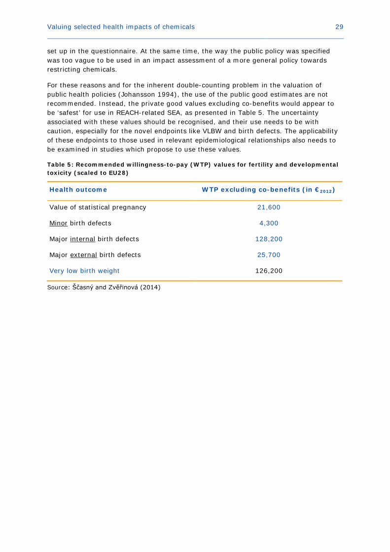
Valuing selected health impacts of chemicals 29
set up in the questionnaire. At the same time, the way the public policy was specified was too vague to be used in an impact assessment of a more general policy towards restricting chemicals.
For these reasons and for the inherent double-counting problem in the valuation of public health policies (Johansson 1994), the use of the public good estimates are not recommended. Instead, the private good values excluding co-benefits would appear to be ‘safest’ for use in REACH-related SEA, as presented in Table 5. The uncertainty associated with these values should be recognised, and their use needs to be with caution, especially for the novel endpoints like VLBW and birth defects. The applicability of these endpoints to those used in relevant epidemiological relationships also needs to be examined in studies which propose to use these values.
Table 5: Recommended willingness-to-pay (WTP) values for fertility and developmental toxicity (scaled to EU28)
Health outcome WTP excluding co-benefits (in €2012)
Value of statistical pregnancy 21,600
Minor birth defects 4,300
Major internal birth defects 128,200
Major external birth defects 25,700
Very low birth weight 126,200
Source: Ščasný and Zvěřinová (2014)

Valuing selected health impacts of chemicals 30
4. Cancer
4.1 Definition of endpoints to be valued
The fourth part of the ECHA study attempted to estimate WTP values associated with reducing the risk of developing and dying from cancer, which might be linked to factors such as exposure to hazardous chemicals. In close cooperation with ECHA staff members, it was decided that the study should focus on unspecified cancer described in terms of generic attributes. This was to avoid any ‘labelling’ by respondents and to reduce the possibility that their responses might be affected by prior perceptions of specific cancer types (Cameron et al. 2009). ‘Generic cancer’ was also deemed to be potentially more transferable across different chemicals and policy contexts and, hence, more generally useful for applications of SEA. It was hoped that any variation in WTP in response to changes in attribute levels might enable valuation for a specific cancer to be ‘constructed’ by inputting its specific attribute levels into the estimated valuation function. This would, however, depend on the sensitivity of WTP to the descriptive attributes and the ability of the valuation exercise to measure it.
The following health outcomes and cancer attributes were selected for the study:
• Probability of getting cancer within the next five years;
• Probability of survival five years after diagnosis;
• Effects on everyday activities of having and being treated for cancer;
• Pain and discomfort from having and being treated for cancer.
A fifth attribute initially considered was the probability of recurrence, i.e. the worry (both in anticipation of getting cancer and when living with the disease) that cancer might always ‘come back’ could well be a significant driver of the ‘dread’ which is often expressed in attitudinal studies on the subject. However, piloting suggested that the cognitive and informational burden for respondents was already significant without this final attribute and so it was not included.
4.2 Description of the study and main results
WTP values were elicited from a sample of the adult population aged 45-60 in four EU Member States: the Czech Republic, Italy, the Netherlands and the U.K. Participants were presented with statistics on cancer risks and survival rates, which were tailored to the age group of the sample so that they reflected the cancer risk the respondent actually faced. Information describing the impacts of cancer on health, daily activities, and quality of life was also given. Respondents were then asked to choose in seven successive binary choice questions between the ‘status quo situation’ – described as involving a given five-year risk of developing cancer and a given five-year survival rate, as well as a level of pain and impact on daily activities – or an option which would involve different levels of these characteristics as well as an annual cost to be paid by the respondent over the next five years.
How the cancer risk reduction would be achieved was not specified in detail. Participants had previously been presented with information and questions about possible actions that could reduce cancer, but for WTP questions they were simply told:

Valuing selected health impacts of chemicals 31
‘Most of these actions cost money. For example, medical tests for early detection of cancer imply some costs, even maybe just in terms of the time and effort required to go and have the test. Replacing certain chemicals in products may likewise increase the cost and hence the price of some of the goods you buy. We would like to ask you to choose between one hypothetical action and the current situation.’
To visualise the changes in the risk of developing cancer, respondents were shown the elicitation instrument depicted in Figure 2.25 The different attributes describing the severity of cancer symptoms were varied across successive questions and across respondents. The risk and cost attributes did vary between any pair of choice options. Importantly, in the first three choice cards either the incidence rate or the survival rate was kept fixed; in the subsequent four choice cards both rates varied between the status quo and the alternative option.
In total 3,888 respondents were interviewed providing 3,407 valid interviews. Respondents who completed the survey in an unreasonably short time (defined by the study authors to be less than 13 minutes) and those who answered the probability screening question incorrectly were excluded from the analysis. Potential protesters (those who were unwilling to express a WTP in any of the choice questions) were not excluded, however, so that the results provide lower-bound estimates of WTP.26 For policy purposes, the WTP for reducing the chance of developing cancer was scaled to represent the value of a statistical case of cancer (VSCC).27 Examining how choices are affected by changes in both probabilities, that of developing cancer and that of surviving cancer, enables WTP for reductions in the unconditional mortality risk (i.e., in the risk of dying from cancer) to be computed, from which the value of a statistical life (VSL) was derived.
WTP values for the pooled sample of four EU Member States were estimated from the random effects probit model using the first three choice cards only.28 The central VSCC estimate reported in the ECHA study is €335,000 and the corresponding VSL amounts to €4.27m (both expressed in €2012). Among the four EU Member States, the respondents from Italy stated the highest and the Czech respondents stated the lowest WTP for reducing the risk of developing cancer, implying the highest and the lowest values of VSCC and VSL, respectively. The set of EU-wide WTP values (in €2012 PPP) recommended by Alberini and Ščasný (2014) are reported in Table 6. They were derived based on
25 Risk visualisation has shown to be effective in reducing inconsistencies of stated-preference based WTP values (Corso et al. 2001). 26 There is an abundant literature, but no general agreement on how to deal with protest answers in stated-preference studies (Jorgensen et al. 1999). While excluding protesters might yield more precise WTP estimates, it is often impossible to identify them because the choice of the status quo option in all seven choice cards can be perfectly consistent with a respondent’s real preferences or a mere expression of survey dismissal. 27 The VSCC is defined as the marginal value of a change in cancer incidence keeping the survival rate fixed (Alberini and Ščasný, 2014: p. 31). As such, it comprises two aspects: the valuation of the illness impacts on the quality of life and of cancer mortality. However, the additive model (without interaction between incidence and survival rate) estimated by Alberini and Ščasný does not allow to back out the relative shares of these components. 28 The random effects probit model controls for unobserved individual preferences that affect the series of binary choices made by one and the same respondent (Wooldridge, 2010).

Valuing selected health impacts of chemicals 32
population-weighted WTP computed for each EU Member State and based on the purchasing power-adjusted unit value benefit transfer of WTP estimates, assuming an income elasticity of WTP of 0.7.29 The level of pain associated with cancer, and the impact that it could have on an individual’s ability to carry on with life, were not significant determinants of respondents’ WTP (neither statistically significant nor significant in size), and hence these factors do not feature in the recommended values.
Table 6: Recommended willingess-to-pay values for cancer risk reduction (scaled to EU28)
Original results €2012
Value of statistical life (VSL) 5,000,000
Value of a statistical case of cancer (VSCC) 396,000
Values based on robustness check
Value of statistical life (VSL) 3,500,000
Value of a statistical case of cancer (VSCC) 350,000
Value of cancer morbidity (VCM) 410,000
Sources: Alberini and Ščasný (2014) and re-estimation carried out by ECHA (see Appendix)
Figure 2: The cancer value elicitation instrument in the ECHA study
29 An income elasticity of 0.7 is well within the range of empirical VSL results (Hammitt and Robinson 2011).

Valuing selected health impacts of chemicals 33
4.3 Evaluation of the results
The analysis produced the following findings. In each Member State, respondents were willing to pay more for larger reductions in the chance of getting cancer and for larger improvements in the chance of surviving it. The coefficients on these regressors were positive and highly significant. The likelihood of accepting a risk-reducing alternative decreased, all else being equal, as the price of that alternative increased. This is the most basic test of the validity of the estimated values. The described pain and impacts on quality of life from cancer did not change the estimated VSL or VSCC, however. Even in the few model specifications in which the corresponding coefficients were statistically significant, no significant changes in the magnitudes of the VSL or VSCC were implied. This is counter to much (although not all) of the existing evidence on attitudes to and the value of reducing cancer risks.30
The failure of the ECHA study to find an effect of symptoms on the valuation of cancer risks could reflect a range of factors. First, the level of information about pain and quality of life impacts provided to respondents was relatively general, and the degree of gradation in the pain and quality of life attributes in the valuation exercise was limited. For instance, the generic information which was provided to respondents on the possible impacts of cancer is presented in Box 1. Thus, information about severity of impacts, durations, levels of pain and capability and so on was intentionally left quite vague, reflecting the ‘generic’ nature of the descriptions but also the significant variation in these aspects which can occur across different cases of cancer.
Second, the attributes and levels covering quality of life and pain in the binary choice questions were specified in very simple terms (Table 7). Two levels of pain – ‘mild’ and ‘moderate’ – were included, and quality of life impacts were described in four simple ways: ‘fully active’, ‘no heavy physical work’, ‘unable to work’ and ‘confined to bed half of the time’. No further information was provided on effects, treatment, duration, and so forth.
30 Jones-Lee et al. (1985) said that people ‘make a significant distinction between different ways of dying and would be willing to pay substantial sums to avoid protracted period of pain prior to cancer death.’ DG Environment (2000) stated that, ‘people may be willing to pay more to reduce their risk of dying from cancer than to reduce their risk of a fatal heart attack, because death from cancer may be preceded by a long period of serious illness.’ A recent (admittedly small) study funded by the UK Health and Safety Executive (Chilton et al. 2013) aimed specifically at understanding the drivers of cancer valuation. It found that the premium for cancer risks over road accident risks disappeared once relative cancer morbidity fell to zero. Similarly, Hammitt and Haninger (2010) found a WTP premium for morbidity, but this applied whether the disease being valued was cancer or not. A meta-analysis of value of life estimated undertaken for the OECD (Lindhjem et al. 2011) found no consistent evidence of a cancer premium once study quality had been controlled for.
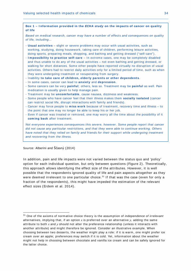
Valuing selected health impacts of chemicals 34
Source: Alberini and Ščasný (2014)
In addition, pain and life impacts were not varied between the status quo and ‘policy’ option for each individual question, but only between questions (Figure 2). Theoretically, this approach allows identifying the effect size of the attributes. However, it is well possible that the respondents ignored quality of life and pain aspects altogether as they were deemed irrelevant to one particular choice.31 If that was the case (even for only a fraction of the respondents), this might have impeded the estimation of the relevant effect sizes (Erdem et al. 2014).
31 One of the axioms of normative choice theory is the assumption of independence of irrelevant alternatives, implying that, if an option x is preferred over an alternative y, adding the same attribute to both x and y should not alter the preference relationship (unless it interacts with another attribute) and might therefore be ignored. Consider an illustrative example. When choosing between two desserts, the weather might play a role: if it is warm, one might prefer ice cream over an apple; preferences may switch if it is cold. Yet, information about the weather might not help in choosing between chocolate and vanilla ice cream and can be safely ignored for the latter choice.
Box 1 – Information provided in the ECHA study on the impacts of cancer on quality of life
Based on medical research, cancer may have a number of effects and consequences on quality of life, including…
- Usual activities – slight or severe problems may occur with usual activities, such as working, studying, doing housework, taking care of children, performing leisure activities, doing sports, preparing meals, shopping, and bathing and getting dressed (“self-care”).
- Impossibility to practice self-care – In extreme cases, one may be completely disabled and thus unable to do any of the usual activities – not even bathing and getting dressed, or walking for short distances. Some other people have reported virtually no disruption of usual activities. Others had to restrict daily activities only for a limited period of time, such as when they were undergoing treatment or recuperating from surgery.
- Inability to take care of children, elderly parents or other dependents. - In some cases, cancer can lead to anxiety and depression. - Some cancers can be very painful; others, less so. Treatment may be painful as well. Pain
medication is usually given to help manage pain. - Treatment may be uncomfortable, cause nausea, dizziness and weakness. - Some people who have cancer feel that their illness makes them socially isolated (cancer
can restrict social life, disrupt interactions with family and friends). - Cancer may force people to miss work because of treatment, recovery time and illness – to
the point that one may no longer be able to keep his or her job. - Even if cancer was treated or removed, one may worry all the time about the possibility of it
coming back after treatment.
Not everyone experiences consequences this severe, however. Some people report that cancer did not cause any particular restrictions, and that they were able to continue working. Others have noted that they relied on family and friends for their support while undergoing treatment and recovering from the illness.
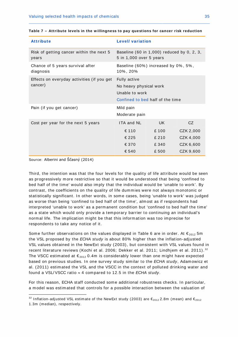
Valuing selected health impacts of chemicals 35
Table 7 – Attribute levels in the willingness to pay questions for cancer risk reduction
Attribute Level/variation
Risk of getting cancer within the next 5 years
Baseline (60 in 1,000) reduced by 0, 2, 3, 5 in 1,000 over 5 years
Chance of 5 years survival after diagnosis
Baseline (60%) increased by 0%, 5%, 10%, 20%
Effects on everyday activities (if you get cancer)
Fully active
No heavy physical work
Unable to work
Confined to bed half of the time
Pain (if you get cancer) Mild pain
Moderate pain
Cost per year for the next 5 years ITA and NL UK CZ
€ 110
€ 225
€ 370
€ 540
£ 100
£ 210
£ 340
£ 500
CZK 2,000
CZK 4,000
CZK 6,600
CZK 9,600
Source: Alberini and Ščasný (2014)
Third, the intention was that the four levels for the quality of life attribute would be seen as progressively more restrictive so that it would be understood that being ‘confined to bed half of the time’ would also imply that the individual would be ‘unable to work’. By contrast, the coefficients on the quality of life dummies were not always monotonic or statistically significant. In other words, in some cases, being ‘unable to work’ was judged as worse than being ‘confined to bed half of the time’, almost as if respondents had interpreted ‘unable to work’ as a permanent condition but ‘confined to bed half the time’ as a state which would only provide a temporary barrier to continuing an individual’s normal life. The implication might be that this information was too imprecise for respondents to take any notice of it.
Some further observations on the values displayed in Table 6 are in order. At €2012 5m the VSL proposed by the ECHA study is about 80% higher than the inflation-adjusted VSL values obtained in the NewExt study (2003), but consistent with VSL values found in recent literature reviews (Kochi et al. 2006; Dekker et al. 2011; Lindhjem et al. 2011).32 The VSCC estimated at €2012 0.4m is considerably lower than one might have expected based on previous studies. In one survey study similar to the ECHA study, Adamowicz et al. (2011) estimated the VSL and the VSCC in the context of polluted drinking water and found a VSL/VSCC ratio ≈ 4 compared to 12.5 in the ECHA study.
For this reason, ECHA staff conducted some additional robustness checks. In particular, a model was estimated that controls for a possible interaction between the valuation of 32 Inflation-adjusted VSL estimate of the NewExt study (2003) are €2012 2.8m (mean) and €2012
1.3m (median), respectively.
Valuing selected health impacts of chemicals 36
an improved survival rate (conditional on having cancer) and the valuation of reductions in the incidence rate of cancer (Rheinberger et al. 2015).33 This is important because the two rates are not independent of each other: any improvement in survival chances will devaluate a reduction in the incidence rate and the other way around. The VSCC and VSL estimates obtained from the additional analysis are in the order of €2012 0.35m and €2012
3.5m, respectively. The implied VSL/VSCC ratio remains substantially higher than those found in the Adamowicz et al. study. As shown in the appendix, the additional regressions include an interaction term between survival chance and incidence rate. The results can thus be used to construct a value of cancer morbidity defined as the marginal value of reducing the cancer incidence rate while keeping unconditional mortality fixed. As displayed in Table 6, this value is estimated to be €2012 0.41m.34
It is important to mention that, because of the way the estimates are constructed, WTP values obtained from the regression analysis are sensitive to small variations in the parameter estimates. As a consequence, even if changes in the regression specifications produced relatively minor changes in parameter estimates, the VSL and VSCC obtained can change significantly. Therefore, instead of recommending a single value, Table 6 recommends two sets of values that can be used in the practical work relating to socio-economic analysis.
4.4 Evidence from the existing literature
The external validity of the ECHA study can be assessed by comparison with earlier research on the value of cancer risk reduction. Alberini and Ščasný (2014) identified in total 53 WTP studies on cancers, 45 of them employing stated preference approaches, seven revealed preferences and one comparing both (and there have been additional publications since their report was completed). Overall, 20 studies dealt with non-specific cancer, generally stated preference studies often in conjunction with other health outcomes (e.g., road accident death, respiratory and/or cardiovascular illness, etc.). Among specific types of cancers, lung cancer was most frequently studied (12 studies), followed by skin cancer (seven studies), leukaemia (three studies), and other (mainly organ) cancers (colon, bladder, uterus, colorectal, stomach, ovarian, lymph etc.).
Cancer is often associated with suffering and pain, and evidence suggests people generally associate it with ‘dread’ (Starr 1969; Fischhoff et al. 1978; Slovic 1987) without necessarily specifying exactly what is meant by the term. This is often taken to imply that the VSL should be higher when the cause of death is cancer rather than other factors such as road accidents (Sunstein 1997; Revesz 1999; U.S. EPA 2000b). Some studies have indeed found that people favour programmes that reduce cancer mortality compared with programmes targeting other risks, but others report no evidence for such a ‘cancer premium.’ Alberini and Ščasný (2014) summarise:
• Savage (1993) found significantly (two to three times) higher WTP for cancer risk compared with various types of accident risk;
33 Details on the sensitivity analysis are presented in the appendix. 34 The value of cancer morbidity is derived from the VSCC evaluated at the survival rate that keeps unconditional mortality constant. As the survival rate has to decrease to outweigh the reduction in the incidence rate, the value of cancer morbidity is actually larger than the VSCC.
Valuing selected health impacts of chemicals 37
• Magat et al. (1996) found their median subject to be indifferent between death from lymph cancer and death in an automobile accident;
• Shackley and Donaldson (2002) found significant differences between mean WTP for a cancer programme and two other programmes;
• Hammitt and Liu (2004) found a cancer premium of about 30 per cent compared with non-cancer degenerative disease, but the result was not statistically significant at conventional levels;
• Tsuge et al. (2005) estimated a cancer premium of about 20 per cent but concluded that there was no need to adjust the VSL for different types of mortality risk, so long as they were appropriately specified in terms of factors such as timing and population characteristics;
• Van Houtven et al. (2008) found a significant cancer premium compared with road accident death, of approximately three times with a five-year latency, declining to 50 per cent with a 25-year latency;
• Hammitt and Haninger (2010) found evidence of a ‘morbidity premium’, but no statistically significant differences in WTP between cancer and other diseases, or with respect to the affected organ, once this was taken into account;
• Alberini and Ščasný (2011) found the VSL to vary by cause of death with a premium for cancer of up to 150 per cent;
• Adamowicz et al. (2011) found a modest cancer ‘discount’ (about 15 per cent) in a trade-off between bladder cancer risk and microbial death risk reduction in drinking water;
• Chestnut et al. (2012) found the cause of death (cancer or heart attack) insignificant in determining WTP for reducing mortality risks through out-of-pocket costs for health-care programmes;
• Cameron and DeShazo (2013) estimated a structural model, which specified a range of named diseases (including various cancers) in terms of common attributes such as morbidity, baseline risk and risk reduction, effect on life expectancy, etc. They found that respondents generally preferred to reduce the risks of future death preceded by one year or five years of illness than the risk of immediate death, due to a relatively very high value being placed on avoiding morbidity;
• Cameron et al. (2009) used a similar model as Cameron and DeShazo (2013) and found that, after controlling for common attributes, the labels attached to a disease profile could have a significant impact on the valuation attached to a risk reduction. For instance, sudden death from breast and prostate cancer was valued at a VSL-equivalent of around $8m, whereas sudden death from lung and skin cancer was valued an order of magnitude less than that.
As Alberini and Ščasný (2014) conclude, studies on the topic have resulted in a rather mixed picture as to whether the cancer VSL is higher than the VSL for other causes of death. Unfortunately, few of these studies provided detailed descriptions of the nature of cancer risks and the implications of the disease. Often they relied only on ‘labels’ to differentiate between disease types, and left respondents to ‘fill in the gaps’ about what they felt the impacts of the disease would be. Then, even if some sort of cancer ‘premium’ is discovered, it is difficult to explain why it exists or what drives it. The clearest example of this is the Cameron et al. (2009) study just mentioned, which found,

Valuing selected health impacts of chemicals 38
for instance, that a 60 year old individual valued a reduction in the risk of death from breast cancer, with a 10-year latency period and with five years’ worth of illness preceding it, at an effective VSL of $4m, but the same disease labelled as ‘skin cancer’ was valued at essentially $0. The authors concluded that this and similar results were evidence that we should value different illnesses differently. Yet it is difficult to reconcile with rationale behaviour that reductions in the risk of dying from skin cancer are deemed worthless, when the same risk is valued at a VSL-equivalent of $4m if it is called breast cancer.
Where disease morbidity is identified and described separately from the risk of mortality, this has often been associated with finding no significant difference in the value of cancer mortality risks compared with other diseases (e.g., Hammitt and Haninger 2010; Adamowicz et al. 2011; Chilton et al. 2013). This does not imply that a cancer premium would not exist – only that it is accounted for by differences in the morbidity attributes of cancer compared with other diseases. This is consistent with a hedonic model of disease valuation, with the value attached to any specific disease being driven by its specific characteristics.
As might be expected, the literature covering quality of life estimates of the impacts of cancer is considerable, and it is not possible to provide a comprehensive survey within the scope of this report. Literature reviews (not specific to cancer) have previously been undertaken by Tengs and Wallace (2000), Morimoto and Fukui (2002), and Tarride (2010). Moreover, ECHA commissioned a review of the principal ‘collections’ of QALY and DALY estimates related to REACH health endpoints, including cancer (RPA 2015). The following broad observations might be made to summarise this extensive literature. The impacts of cancer on quality of life seem to represent a ‘discount’ on full health of between 10 and 50 per cent, with most effect sizes between 20 and 40 per cent (i.e., QALY weights around 0.6-0.8, and DALY weights around 0.2-0.4. There are no obviously ‘worse’ cancers, with perhaps the exception of lung cancer. Impacts also vary with the stage of the cancer, implying more severe impacts for metastatic and terminal cancers.
These weights relate only to the impact on the quality of life from suffering a particular cancer at a particular stage. They do not directly represent the quality of life impact of a case of cancer. Estimating a value for a case of cancer therefore requires knowledge of the durations of the stages and the prognosis of the disease, and this information is less readily reported in the literature. As a result, quality of life values for specific cancers would generally need to be constructed on a case-by-case basis following research on the treatment and prognosis for each particular type of cancer. As many cancers progress fast, however, this valuation approach leads to somewhat lower impact values. An upper bound on the utility loss from cancer may be derived by assuming a maximum length of five years over which the sufferer might lose 0.4*5 = 2 QALYs. To monetise, one can multiply this QALY loss by the NewExt median VOLY of €64,000 and by a VOLY of €290,000 corresponding to the VSL of €5 m as recommended by the ECHA study.35 This binds the money value of the cancer-induced QALY loss to a range between
35 The VOLY can be derived from annuitizing the VSL (Aldy and Viscusi 2008): 𝑉𝑉𝑉𝑉𝑉𝑉𝑉𝑉 = 𝑟𝑟𝑉𝑉𝑟𝑟𝑉𝑉/(1 −(1 + 𝑟𝑟)−𝐿𝐿𝐿𝐿), where the discount rate is set to 𝑟𝑟 = 4% and the remaining life expectancy (LE) of EU citizens aged 45-60 ranges according to Eurostat from 37 years (at age 45) to 24 years (at age 60). For a VSL of € 5m and a remaining life expectancy of 30 years, the implied VOLY is about €
290,000.

Valuing selected health impacts of chemicals 39
€128,000 and €580,000, indicating that the order of magnitude of the estimated VSCC and the corresponding value of cancer morbidity is plausible.
4.5 Recommended values for the prevention of cancer
The literature relating to the impact of cancer on quality of life and on the valuation of cancer risks is extensive. Regarding the latter, it is perhaps surprising that – despite the widely accepted ‘orthodoxy’ that cancer risks are viewed with ‘dread’ by the general population – there is no clear agreement on the existence or value of a ‘premium’ on reducing cancer risks compared with other sources of risk to health and life. However, many cancer risk valuation studies have not been designed (intentionally or unintentionally) in a way that gives respondents a full description of the impacts different types of cancer might have on their health, instead providing ‘labels’ and relying on respondents’ own perceptions. Although it is sometimes argued that it is individuals’ own perceptions of health risks which should count most, the discussion in the previous section demonstrates the potential for common perceptions of the impacts of cancer to be biased.
Unless it can be demonstrated that individuals who base their preferences for cancer risk reduction on perceived rather than statistical risks experience real reductions in their utility as a result of their perception – perhaps as a form of worry about becoming a victim of cancer36 – then these preferences might simply reflect a misperception of the possible future impacts of cancer, not a real reduction in individual welfare. It is the actual impacts of cancer on health, and the reductions in welfare associated with them, which are relevant for regulatory impact assessment, and the QALY literature demonstrates that these are real and significant (albeit possibly not as significant as people often suspect). Valuation studies that separate out the mortality and morbidity impacts of cancer tend to find that differences in the valuation of cancer and other risks to life disappear. This suggests that the value of any premium attached to cancer risks in SEA under REACH should be driven by cancer morbidity, i.e. reflecting that any fatal cancer is preceded by a period of illness.
Given the above estimate of the utility loss from cancer based on monetised QALYs, it might be argued that morbidity-induced drops in life quality are smaller than the estimated VSCC and value of cancer morbidity. However, that benefit transfer was done only for illustrative purposes, and it is not clear how reliable it is. Plus, the WTP values might be interpreted to also capture anxiety and other psychological costs related to a survived cancer, on which one would implicitly place zero value if one would monetise the illness effects of non-fatal cancers only. Therefore, a more comprehensive valuation of cancer morbidity might be a suitable topic for future research. A similar exercise has been undertaken by the UK HSE (Chilton et al., 2013).
The WTP values related to cancer as presented in Table 6 can be used in SEA under REACH in the following way. Every fatal cancer case is preceded by a period of latency and a (possibly very short) duration of illness. Hence, the number of excess cancer cases derived from dose-response modelling needs to be adjusted in order to reflect for latency, duration of illness and cancer-specific survival chances. Box 2 provides one example on how the values might be used in practice.
36 In which case they should be observable and, presumably, could be valued directly.
Valuing selected health impacts of chemicals 40
In a nutshell, we may summarise the following valuation principles for cancer risk. The higher is the risk of death in the event of cancer, the higher is the value of avoiding cancer. The value of avoiding cancer is positively correlated with the value of cancer morbidity and related opportunity costs of actually having cancer, as well as the risks of recurrence (with its associated costs).37 The value of avoiding cancer is negatively correlated with the survival chance if one has cancer. In other words, people are willing to pay more for avoiding lung cancer than they are willing to pay for avoiding some types of systemic cancer because the survival prospects for the latter are much better than for the former.
37 As Hammitt and Haninger (2010) point out, death from cancer might not be considered uniformly worse than death from other causes – for instance, receiving ‘notice’ of death might provide an opportunity for ‘setting one’s house in order’. However, the fact that evidence suggests people fear cancer death more than other deaths, and that in 2014 a former editor of the British Medical Journal felt the need to argue in favour of cancer deaths for this very reason (Smith, 2014), suggest that the morbidity costs of cancer are generally viewed as being negative in net terms.
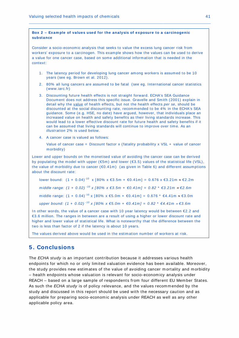
Valuing selected health impacts of chemicals 41
5. Conclusions
The ECHA study is an important contribution because it addresses various health endpoints for which no or only limited valuation evidence has been available. Moreover, the study provides new estimates of the value of avoiding cancer mortality and morbidity – health endpoints whose valuation is relevant for socio-economicy analysis under REACH – based on a large sample of respondents from four different EU Member States. As such the ECHA study is of policy relevance, and the values recommended by the study and discussed in this report should be used with the necessary caution and as applicable for preparing socio-economic analysis under REACH as well as any other applicable policy area.
Box 2 – Example of values used for the analysis of exposure to a carcinogenic substance Consider a socio-economic analysis that seeks to value the excess lung cancer risk from workers’ exposure to a carcinogen. This example shows how the values can be used to derive a value for one cancer case, based on some additional information that is needed in the context:
1. The latency period for developing lung cancer among workers is assumed to be 10 years (see eg. Brown et al. 2012).
2. 80% all lung cancers are assumed to be fatal (see eg. International cancer statistics (www.iarc.fr)
3. Discounting future health effects is not straight forward. ECHA’s SEA Guidance Document does not address this specific issue. Gravelle and Smith (2001) explain in detail why the value of health effects, but not the health effects per se, should be discounted at the social discounting rate, recommended to be 4% in the ECHA’s SEA guidance. Some (e.g. HSE, no date) have argued, however, that individuals place an increased value on health and safety benefits as their living standards increase. This would lead to a lower effective discount rate for future health and safety benefits if it can be assumed that living standards will continue to improve over time. As an illustration 2% is used below.
4. A cancer case is valued as follows:
Value of cancer case = Discount factor x (fatality probability x VSL + value of cancer morbidity)
Lower and upper bounds on the monetised value of avoiding the cancer case can be derived by populating the model with upper (€5m) and lower (€3.5) values of the statistical life (VSL), the value of morbidity due to cancer (€0.41m) (as given in Table 6) and different assumptions about the discount rate:
lower bound: (1 + 0.04)-10 x [80% x €3.5m + €0.41m] = 0.676 x €3.21m ≈ €2.2m
middle range: (1 + 0.02) -10 x [80% x €3.5m + €0.41m] = 0.82 * €3.21m ≈ €2.6m
middle range: (1 + 0.04)-10 x [80% x €5.0m + €0.41m] = 0.676 * €4.41m ≈ €3.0m
upper bound: (1 + 0.02) -10 x [80% x €5.0m + €0.41m] = 0.82 * €4.41m ≈ €3.6m
In other words, the value of a cancer case with 10 year latency would be between €2.2 and €3.6 million. The ranges in between are a result of using a higher or lower discount rate and higher and lower value of statistical life. What is noteworthy that the difference between the two is less than factor of 2 if the latency is about 10 years.
The values derived above would be used in the estimation number of workers at risk.
Valuing selected health impacts of chemicals 42
Appendix – Robustness Check of the values derived for cancer
In the choice tasks exemplified by Figure 2 respondents had to do two things at the same time. They had to value jointly the reductions in the risk of developing cancer and/or increases in the likelihood of surviving, conditional on developing cancer in the first place. The unconditional risk of dying from cancer is affected by (Rheinberger et al. 2015): (i) the chance of developing cancer; (ii) the chance of dying conditional on having cancer. Therefore, a reduction in the unconditional risk of dying from cancer is attained by reducing (i), reducing (ii), or reducing (i) and (ii) at the same time.
A reduction in unconditional mortality risk is the appropriate risk change in the context of computing the VSL. Define 𝐼𝐼0 as the incidence rate of cancer under the status quo, and 𝐼𝐼1 ≤ 𝐼𝐼0 as the incidence rate of cancer if the proposed intervention is implemented. Hence, ∆𝐼𝐼 = 𝐼𝐼0 − 𝐼𝐼1 ≥ 0. Similarly, define 𝑟𝑟0 as the chance of surviving cancer under the status quo, and 𝑟𝑟1 as the chance of surviving cancer with the intervention implemented. As 𝑟𝑟1 ≥ 𝑟𝑟0, we have that ∆𝑟𝑟 = 𝑟𝑟1 − 𝑟𝑟0 ≥ 0. The unconditional risk of dying (i.e., the mortality risk) under the status quo is 𝑀𝑀0 = 𝐼𝐼0(1 − 𝑟𝑟0); the corresponding unconditional risk of dying with the intervention implemented is 𝑀𝑀1 = 𝐼𝐼1(1 − 𝑟𝑟1).38 Therefore, the reduction in the unconditional risk of dying of cancer equals:
∆𝑀𝑀 = 𝑀𝑀0 −𝑀𝑀1 = 𝐼𝐼0(1 − 𝑟𝑟0) − 𝐼𝐼1(1 − 𝑟𝑟1) = ∆𝐼𝐼 − (𝐼𝐼0𝑟𝑟0 − 𝐼𝐼1𝑟𝑟1) =
∆𝐼𝐼 − 𝐼𝐼0𝑟𝑟0 + (𝐼𝐼0 − ∆𝐼𝐼)(𝑟𝑟0 + ∆𝑟𝑟) = (1 − 𝑟𝑟0)∆𝐼𝐼 + 𝐼𝐼0∆𝑟𝑟 − ∆𝐼𝐼∆𝑟𝑟.
If the status quo is fixed (i.e., 𝐼𝐼0 and 𝑟𝑟0 are constant), then ∆𝑀𝑀 is a positive quantity.39 An indirect utility function consistent with the definition of VSL (Hammitt 2000) would thus be 𝑉𝑉 = 𝛼𝛼∆𝑀𝑀 + 𝛽𝛽(𝑦𝑦 − 𝐶𝐶), based on which one obtains 𝑉𝑉𝑟𝑟𝑉𝑉 = −(𝜕𝜕𝑉𝑉/𝜕𝜕∆𝑀𝑀)/(𝜕𝜕𝑉𝑉/𝜕𝜕𝐶𝐶) = −𝛼𝛼/𝛽𝛽. One can replace ∆𝑀𝑀 with its three components in the right hand side of the above equation, in which case one obtains 𝑊𝑊 = 𝛼𝛼∆𝐼𝐼 + 𝛾𝛾∆𝑟𝑟 − 𝛿𝛿(∆𝐼𝐼∆𝑟𝑟) + 𝛽𝛽(𝑦𝑦 − 𝐶𝐶), since 𝑟𝑟0 and 𝐼𝐼0 are constants. Taking the partial derivatives of the 𝑊𝑊(. ) function with respect to ∆𝑟𝑟 and ∆𝐼𝐼 yields alternative expressions for the VSL and VSCC, respectively. In particular, one has:
𝑉𝑉𝑟𝑟𝑉𝑉 = −𝜕𝜕𝜕𝜕𝜕𝜕∆𝑆𝑆𝜕𝜕𝜕𝜕𝜕𝜕𝜕𝜕
�∆𝐼𝐼=0
= −𝛾𝛾−𝛿𝛿∆𝐼𝐼𝛽𝛽
= − 𝛾𝛾𝛽𝛽, and
𝑉𝑉𝑟𝑟𝐶𝐶𝐶𝐶 = −𝜕𝜕𝜕𝜕/𝜕𝜕∆𝐼𝐼𝜕𝜕𝜕𝜕/𝜕𝜕𝜕𝜕
�∆𝑆𝑆=0
= −𝛼𝛼−𝛿𝛿∆𝑆𝑆𝛽𝛽
= −𝛼𝛼𝛽𝛽.
By definition, the VSCC equals the marginal value of a reduction in the incidence rate keeping the survival rate fixed. However, this means that the VSCC is composed of two sources of benefits: those arising from not suffering the cancer disease, and those arising from the reduction in the unconditional risk of dying (𝑟𝑟0∆𝐼𝐼). A theoretically sound estimate of the value of cancer morbidity (VCM) can still be constructed by disentangling the two sources of health utility. To do so the VSCC equation needs to be evaluated at 38 In the ECHA study (Alberini and Ščasný 2014), the unconditional probability of dying from cancer is denoted as UNCMORT. 39 In Alberini and Ščasný’s (2014) survey, everyone faced the same initial incidence rate 𝐼𝐼0 (25 in 1000 over 5 years) and survival chance 𝑟𝑟0 (60%)) but ∆𝐼𝐼 and ∆𝑟𝑟 varied across the respondents.
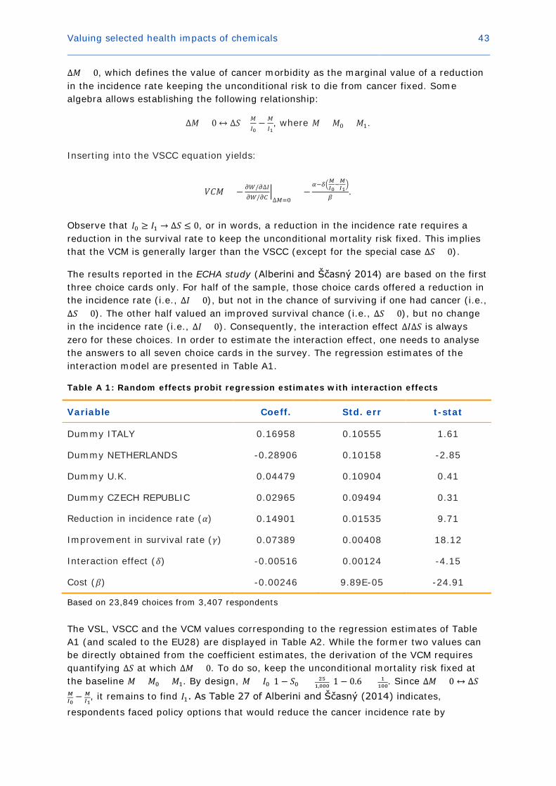
Valuing selected health impacts of chemicals 43
∆𝑀𝑀 = 0, which defines the value of cancer morbidity as the marginal value of a reduction in the incidence rate keeping the unconditional risk to die from cancer fixed. Some algebra allows establishing the following relationship:
∆𝑀𝑀 = 0 ↔ ∆𝑟𝑟= 𝑀𝑀𝐼𝐼0− 𝑀𝑀
𝐼𝐼1, where 𝑀𝑀 = 𝑀𝑀0 = 𝑀𝑀1.
Inserting into the VSCC equation yields:
𝑉𝑉𝐶𝐶𝑀𝑀 = − 𝜕𝜕𝜕𝜕/𝜕𝜕∆𝐼𝐼𝜕𝜕𝜕𝜕/𝜕𝜕𝜕𝜕
�∆𝑀𝑀=0
= −𝛼𝛼−𝛿𝛿�𝑀𝑀𝐼𝐼0
−𝑀𝑀𝐼𝐼1�
𝛽𝛽.
Observe that 𝐼𝐼0 ≥ 𝐼𝐼1 → ∆𝑟𝑟 ≤ 0, or in words, a reduction in the incidence rate requires a reduction in the survival rate to keep the unconditional mortality risk fixed. This implies that the VCM is generally larger than the VSCC (except for the special case ∆𝑟𝑟 = 0).
The results reported in the ECHA study (Alberini and Ščasný 2014) are based on the first three choice cards only. For half of the sample, those choice cards offered a reduction in the incidence rate (i.e., ∆𝐼𝐼 > 0), but not in the chance of surviving if one had cancer (i.e., ∆𝑟𝑟 = 0). The other half valued an improved survival chance (i.e., ∆𝑟𝑟 > 0), but no change in the incidence rate (i.e., ∆𝐼𝐼 = 0). Consequently, the interaction effect ∆𝐼𝐼∆𝑟𝑟 is always zero for these choices. In order to estimate the interaction effect, one needs to analyse the answers to all seven choice cards in the survey. The regression estimates of the interaction model are presented in Table A1.
Table A 1: Random effects probit regression estimates with interaction effects
Variable Coeff. Std. err t-stat
Dummy ITALY 0.16958 0.10555 1.61
Dummy NETHERLANDS -0.28906 0.10158 -2.85
Dummy U.K. 0.04479 0.10904 0.41
Dummy CZECH REPUBLIC 0.02965 0.09494 0.31
Reduction in incidence rate (𝛼𝛼) 0.14901 0.01535 9.71
Improvement in survival rate (𝛾𝛾) 0.07389 0.00408 18.12
Interaction effect (𝛿𝛿) -0.00516 0.00124 -4.15
Cost (𝛽𝛽) -0.00246 9.89E-05 -24.91
Based on 23,849 choices from 3,407 respondents
The VSL, VSCC and the VCM values corresponding to the regression estimates of Table A1 (and scaled to the EU28) are displayed in Table A2. While the former two values can be directly obtained from the coefficient estimates, the derivation of the VCM requires quantifying ∆𝑟𝑟 at which ∆𝑀𝑀 = 0. To do so, keep the unconditional mortality risk fixed at the baseline 𝑀𝑀 = 𝑀𝑀0 = 𝑀𝑀1. By design, 𝑀𝑀 = 𝐼𝐼0(1 − 𝑟𝑟0) = 25
1,000(1 − 0.6) = 1100. Since ∆𝑀𝑀 = 0 ↔ ∆𝑟𝑟=
𝑀𝑀𝐼𝐼0− 𝑀𝑀
𝐼𝐼1, it remains to find 𝐼𝐼1. As Table 27 of Alberini and Ščasný (2014) indicates,
respondents faced policy options that would reduce the cancer incidence rate by
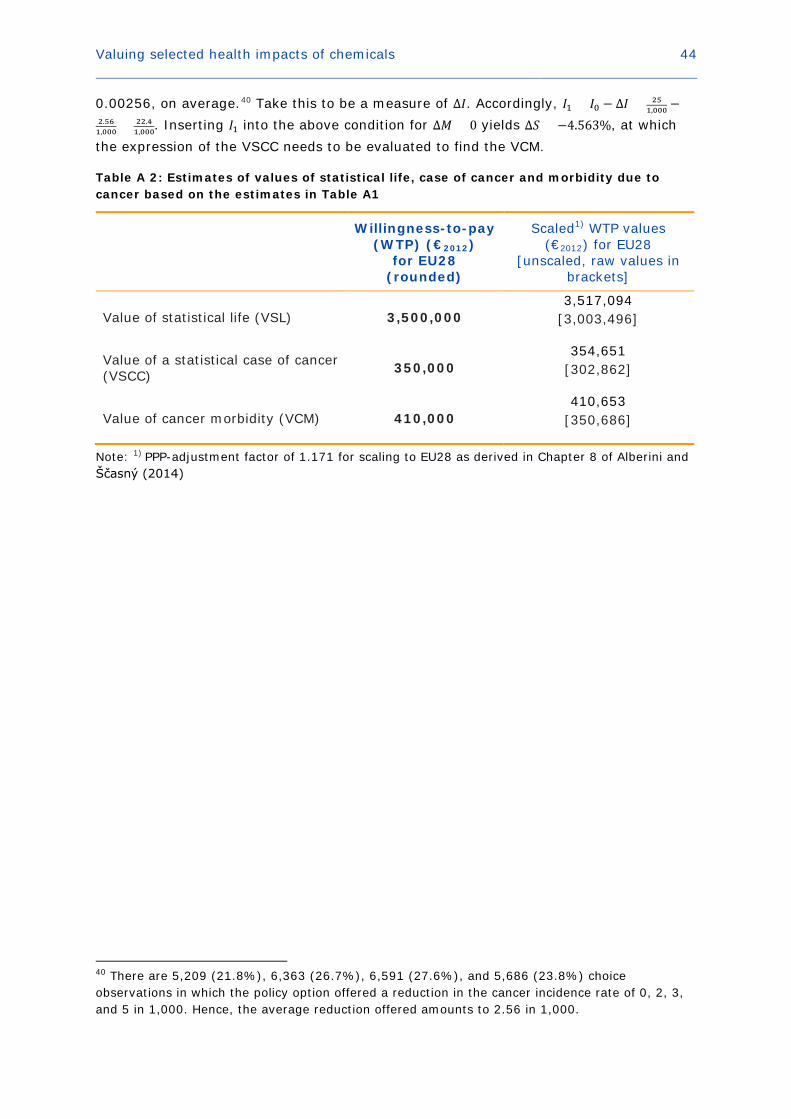
Valuing selected health impacts of chemicals 44
0.00256, on average.40 Take this to be a measure of ∆𝐼𝐼. Accordingly, 𝐼𝐼1 = 𝐼𝐼0 − ∆𝐼𝐼 = 251,000 −
2.561,000 = 22.4
1,000. Inserting 𝐼𝐼1 into the above condition for ∆𝑀𝑀 = 0 yields ∆𝑟𝑟 = −4.563%, at which the expression of the VSCC needs to be evaluated to find the VCM.
Table A 2: Estimates of values of statistical life, case of cancer and morbidity due to cancer based on the estimates in Table A1
Willingness-to-pay (WTP) (€2012)
for EU28 (rounded)
Scaled1) WTP values (€2012) for EU28
[unscaled, raw values in brackets]
Value of statistical life (VSL) 3,500,000 3,517,094
[3,003,496]
Value of a statistical case of cancer (VSCC) 350,000
354,651 [302,862]
Value of cancer morbidity (VCM) 410,000 410,653
[350,686]
Note: 1) PPP-adjustment factor of 1.171 for scaling to EU28 as derived in Chapter 8 of Alberini and Ščasný (2014)
40 There are 5,209 (21.8%), 6,363 (26.7%), 6,591 (27.6%), and 5,686 (23.8%) choice observations in which the policy option offered a reduction in the cancer incidence rate of 0, 2, 3, and 5 in 1,000. Hence, the average reduction offered amounts to 2.56 in 1,000.
Valuing selected health impacts of chemicals 45
References
Adamowicz, W., Dupont, D., Krupnick, A., et al. (2011). Valuation of cancer and microbial disease risk reductions in municipal drinking water: An analysis of risk context using multiple valuation methods. Journal of Environmental Economics and Management, 61(2): 213-226.
Agee, M. D., and Crocker, T. D. (1996). Parental Altruism and Child Lead Exposure: Inferences from the Demand for Chelation Therapy. Journal of Human Resources, 31(3), 677-691.
Alberini, A., and Ščasný, M. (2011). Context and the VSL: Evidence from a Stated Preference Study in Italy and the Czech Republic. Environmental and Resource Economics, 49(4): 511-538.
Alberini, A., and Ščasný, M. (2014). Stated-preference study to examine the economic value of benefits of avoiding selected adverse human health outcomes due to exposure to chemicals in the European Union: Carcinogens, Report for ECHA.
Allgar, V. L., and Neal, R. D. (2005). Delays in the diagnosis of six cancers: analysis of data from the National Survey of NHS Patients. British Journal of Cancer, 92(11): 1959-1970.
Aldy, J. E., and Viscusi, W.K. (2008). Adjusting the Value of Statistical Life for Age and Cohort Effects. Review of Economics and Statistics, 90(3): 573-581.
Blanchette, C. M., Liang, C., Lubeck, D. P., et al. (2015). Progression of autosomal dominant kidney disease: measurement of the stage transitions of chronic kidney disease. Drugs in Context, 4: 212275.
Bosworth, R., Cameron, T. A., and DeShazo, J. R. (2009). Demand for environmental policies to improve health: Evaluating community-level policy scenarios. Journal of Environmental Economics and Management, 57(3): 293-308.
Boulware, L. E., Jaar, B. G., Tarver-Carr, M. E., et al. (2004). Screening for Proteinuria in US Adults. Journal of the American Medical Association, 290(23): 3101-3114.
Brown, T., Cherrie, J., Van Tongeren, M., et al. (2012). The burden of occupational cancer in Great Britain – Lung cancer. Research Report #858, U.K. Health and Safety Executive.
Cameron, T. A., DeShazo, J. R., and Johnson, E. (2009). Willingness to Pay for Health Risk Reductions: Differences by Type of Illness, mimeo, University of Oregon.
Cameron, T. A. and DeShazo, J. R. (2013). Demand for Health Risk Reductions. Journal of Environmental Economics and Management, 65(1): 87-109.
Carson, R. T., and Hanemann, W. M. (2005). Contingent valuation. In Maeler, K.-G. and Vincent, J.R. (eds.): Handbook of Environmental Economics 2, Elsevier: 821-936.
Case, A. P. and Canfield, M. A. (2009). Methods for developing useful estimates of the costs associated with birth defects. Birth Defects Research Part A: Clinical and Molecular Teratology, 85(11): 920-924.
Chestnut, L. G., Rowe, R. D., and Breffle, W. S. (2012). Economic Valuation of Mortality‐Risk Reduction: Stated Preference Estimates from the United States and Canada. Contemporary Economic Policy, 30(3): 399-416.

Valuing selected health impacts of chemicals 46
Chilton, S., Metcalf, H., McDonald, R. (2013). Latency, dread and cancer risks. Report for the UK Health and Safety Executive. January 2013. (unpublished).
Christophers, E., Barker, J., Griffiths, C. E. M., et al. (2010). The risk of psoriatic arthritis remains constant following initial diagnosis of psoriasis among patients seen in European dermatology clinics. Journal of the European Academy of Dermatology and Venereology, 24(5): 548-554.
Corso, P. S., Hammitt, J. K., and Graham, J. D. (2001). Valuing mortality-risk reduction: using visual aids to improve the validity of contingent valuation. Journal of Risk and Uncertainty, 23(2): 165-184.
Dalton, M., and Lilford, R. J. (1989). Benefits of invitro fertilization. Lancet, 2(8675): 1327-1327.
Dekker, T., Brouwer, R., Hofkes, M., et al. (2011). The effect of risk context on the value of a statistical life: a Bayesian meta-model. Environmental and Resource Economics, 49(4): 597-624.
Desaigues, B., Ami, D., Bartczak, A., et al. (2011). Economic valuation of air pollution mortality: A 9-country contingent valuation survey of value of a life year (VOLY). Ecological Indicators, 11(3): 902-910.
Dolan, P., Gudex, C., Kind, P., and Williams, A. (1996). The time trade‐off method: results from a general population study. Health Economics, 5(2): 141-154.
Dolan, P. (1997). Modeling valuations for EuroQol health states. Medical Care, 35(11): 1095-1108.
Erdem, S., Campbell, D., and Thompson, C. (2014). Elimination and selection by aspects in health choice experiments: Prioritising health service innovations. Journal of Health Economics, 38: 10-22.
Feeny, D., Furlong, W., Torrance, G.W., et al. (2002). Multiattribute and single‐attribute utility functions for the health utilities index mark 3 system. Medical Care, 40(2): 113-128.
Fischhoff, B., Slovic, P., Lichtenstein, S., et al. (1978). How safe is safe enough? A psychometric study of attitudes towards technological risks and benefits. Policy Sciences, 9(2): 127-152.
Gardino, S. L., Sfekas, A., and Dranove, D. (2010). Anticipating Ovarian Tissue Cryopreservation in the Health-Care Marketplace: A Willingness to Pay Assessment. Cancer Treatment Research, 156: 363-370.
Gorodetskaya, I., et al. (2005). Health-related quality of life and estimates of utility in chronic kidney disease. Kidney International, 68(6): 2801-2808.
Granberg, M., Wikland, M., Nilsson, L., et al. (1995). Couples’ willingness to pay for IVF/ET. Acta Obstetricia et Gynecologica Scandinavica, 74(3): 199-202.
Gravelle, H., and Smith, D. (2001). Discounting for health effects in cost-benefit and cost-effectiveness analysis. Health Economics, 10(7): 587-599.
Haagsma, J. A., Maertens de Noordhout, C., Polinder, S., et al. (2015). Assessing disability weights based on the responses of 30,660 people from four European countries. Population Health Metrics, 13(1): 10.

Valuing selected health impacts of chemicals 47
Hammitt, J. K. (2000). Valuing mortality risk: theory and practice. Environmental Science & Technology, 34(8): 1396-1400.
Hammitt, J. K. (2013). Admissible Utility Functions for Health, Longevity, and Wealth: Integrating Monetary and Life-Year Measures. Journal of Risk and Uncertainty, 47(3): 311-325.
Hammitt, J. K., and Haninger, K. (2010). Valuing fatal risks to children and adults: Effects of disease, latency, and risk aversion. Journal of Risk and Uncertainty, 40(1): 57-83.
Hammitt, J. K., and Liu, J.-T. (2004). Effects of Disease Type and Latency on the Value of Mortality Risk. Journal of Risk and Uncertainty, 28(1): 73-95.
Hammitt, J. K., and Robinson, L. A. (2011). The income elasticity of the value per statistical life: transferring estimates between high and low income populations. Journal of Benefit-Cost Analysis, 2(1): 1-29.
Hauber, A. B., Gonzalez, J. M., Schenkel, B., et al. (2011). The value to patients of reducing lesion severity in plaque psoriasis. Journal of Dermatological Treatment, 22(5): 266-275.
Herold, D. K. (2010). Patient willingness to pay for a kidney for transplantation. American Journal of Transplantation, 10(6): 1394-1400.
Hutchings, S., and Rushton, L. (2007). Estimation of the Burden of Childhood Disease in Europe due to Environmental Risk Factors. Copenhagen, Denmark: Draft Report to the EEA.
HSE (no date). HSE principles for Cost Benefit Analysis (CBA) in support of ALARP decisions. Available at http://www.hse.gov.uk/risk/theory/alarpcba.htm#footnotes
Jentink, J., Boersma, C., de Jong-van den Berg, L. T., et al. (2012). Economic evaluation of anti-epileptic drug therapies with specific focus on teratogenic outcomes. Journal of Medical Economics, 15(5): 862-868.
Johansson, P. O. (1994). Altruism and the value of statistical life: empirical implications. Journal of Health Economics, 13(1): 111-118.
Jones-Lee, M., Hammerton, M., and Philips, P. (1985). The value of safety: results of a national sample survey. Economic Journal, 95(377): 49-72.
Jorgensen, B. S., Syme, G. J., Bishop, B. J, et al. (1999). Protest Responses in Contingent Valuation. Environmental and Resource Economics, 14(1): 131-150.
Joyce, T. J., Grossman, M., and Goldman, F. (1989). An assessment of the benefits of air pollution control: The case of infant health. Journal of Urban Economics, 25(1): 32-51.
Kahneman, D., and Tversky, A. (1992). Advances in prospect theory: Cumulative representation of uncertainty. Journal of Risk and Uncertainty, 5(4): 297-323.
Kerr, M., Bray, B., Medcalf, J., et al. (2012). Estimating the financial cost of chronic kidney disease to the NHS in England. Nephrology Dialysis Transplantation, 27 (3): 73-80.
Kjær, T., Bech, M., Kronborg, C., et al. (2013). Public preferences for establishing nephrology facilities in Greenland: estimating willingness-to-pay using a discrete choice experiment. European Journal of Health Economics, 14(5): 739-748.
Valuing selected health impacts of chemicals 48
Kochi, I., Hubbell, B., and Kramer, R. (2006). An empirical Bayes approach to combining and comparing estimates of the value of a statistical life for environmental policy analysis. Environmental and Resource Economics, 34(3): 385-406.
Kumar, P., and Burton, B. K. (2008). Congenital malformations: Evidence-based evaluation and management. New York: McGraw-Hill Medical.
Lindhjem, H., Navrud, S., Braathen, N. A., et al. (2011). Valuing Mortality Risk Reductions from Environmental, Transport, and Health Policies: A Global Meta‐Analysis of Stated Preference Studies. Risk Analysis, 31(9): 1381-1407.
Lundberg, L., Johannesson, M., Silverdahl, M., et al. (1999). Quality of life, health‐state utilities and willingness to pay in patients with psoriasis and atopic eczema. British Journal of Dermatology, 141(6): 1067-1075.
Maca, V., et al. (2011). HEIMTSA: Presentation of unit values for health end-points: country-specific and pooled. Report for the European Commission Sixth Framework Programme.
Maca, V., et al. (2014). Stated-preference study to examine the economic value of benefits of avoiding selected adverse human health outcomes due to exposure to chemicals in the European Union: Sensitization and Dose Toxicity. Report for ECHA.
Maca, V., Braun-Kohlová, M., and Navrud, S. (2015). Valuing Environmentally Related Chronic Illnesses – A Multidimensional Scope Sensitivity Analysis. Paper presented at the 2015 annual conference of European Association of Environmental and Resource Economists, Helsinki.
Magat, W. A., Viscusi, W. K., and Huber, J. (1996). A Reference Lottery Metric for Valuing Health. Management Science, 42(8): 1118-1130.
Morimoto, T., and Fukui, T. (2002). Utilities measured by rating scale, time trade-off, and standard gamble: review and reference for health care professionals. Journal of Epidemiology, 12(2): 160-178.
Nastis, S. A., and Crocker, T. D. (2003) Pregnant Mother’s Valuation of Own and Child Health. Paper presented at EAERE: http://www.webmeets.com/files/papers/EAERE/2008/157/157.pdf
Nastis, S. A., and Crocker, T. D. (2012). Valuing mother and child health: The intrauterine environment. Economics and Human Biology, 10(3): 318-328.
NICE (2012). Psoriasis: The assessment and management of psoriasis, National Institute for Health and Clinical Excellence Clinical Guideline #153.
NICE (2013). Fertility: assessment and treatment for people with fertility problems. National Institute for Health and Clinical Excellence Clinical Guideline #156.
Navrud, S. (2001). Valuing health impacts from air pollution in Europe. Environmental and Resource Economics, 20(4): 305-329.
Neri, L., McEwan, P., Sennfält, K., et al. (2012). Characterizing the relationship between health utility and renal function after kidney transplantation in UK and US: a cross-sectional study. Health and Quality of Life Outcomes, 10: 139.
Neumann, P. J., and Johannesson, M. (1994). The willingness to pay for in vitro fertilization: a pilot study using contingent valuation. Medical Care, 32(7): 686-699.

Valuing selected health impacts of chemicals 49
NewExt (2003). New Elements for the Assessment of External Costs from Energy Technologies. Final report. http://www.ier.uni-stuttgart.de/forschung/projektwebsites/newext/newext_final.pdf.
Olesen, J., Gustavsson, A., Svensson, M., et al. [on behalf of the DBE2010 study group and the European Brain Council] (2012). The economic cost of brain disorders in Europe. European Journal of Neurology, 19(1): 155-162.
Olsson, M. (2014). The Cost of Inaction: A Socioeconomic analysis of costs linked to effects of endocrine disrupting substances on male reproductive health. Report to the Nordic Council of Ministers.
Palumbo, A., De La Fuente, P., Rodriguez, M., et al. (2011). Willingness to pay and conjoint analysis to determine women's preferences for ovarian stimulating hormones in the treatment of infertility in Spain. Human Reproduction, 26(7): 1790-1798.
Petrou, S., Abangma, G., Johnson, S., et al. (2009). Costs and health utilities associated with extremely preterm birth: evidence from the EPICure study. Value in Health, 12(8): 1124-1134.
Rautava, L.,Häkkinen, U., Korvenranta, E., et al. (2009). Health-related quality of life in 5-year-old very low birth weight infants. Journal of Pediatrics, 155(3): 338-343.
Ready, R., Navrud, S., Day, B., et al. (2004). Benefit Transfer in Europe: How Reliable Are Transfers between Countries? Environmental and Resource Economics, 29(1): 67-82.
Revesz, R. L. (1999). Environmental Regulation, Cost-Benefit Analysis, and the Discounting of Human Lives. Columbia Law Review, 99(4): 941-1017.
Rheinberger, C.M., Herrera, D., Hammitt, J.K. (2015). Cancer risk valuation: To treat, or to prevent, that is the question! Paper presented at the 2015 annual meeting of the Society for Risk Analysis, Arlington.
RPA (Risk and Policy Analysts) (2015). Quantification and valuation of the human health impacts of chemicals based on quality and disability-adjusted life-years. Report for ECHA.
Ryan, M. (1996). Using willingness to pay to assess the benefits of assisted reproductive techniques. Health Economics, 5(6): 543-558.
Ryan, M. (1997). Should government fund assisted reproductive techniques? A study using willingness to pay. Applied Economics, 29: 841-849.
Ryan, M. (1998). Valuing psychological factors in the provision of assisted reproductive techniques using the economic instrument of willingness to pay. Journal of Economic Psychology, 19: 179-204.
Ryan, M. (1999). Using conjoint analysis to take account of patient preferences and go beyond health outcomes: an application to in vitro fertilisation. Social Science and Medicine, 48(4): 535-546.
Salomon, J. A, Vos, T., Hogan, D. R., et al. (2012). Common values in assessing health outcomes from disease and injury: disability weights measurement study for the Global Burden of Disease Study 2010. Lancet, 380(9859): 2129-2143.
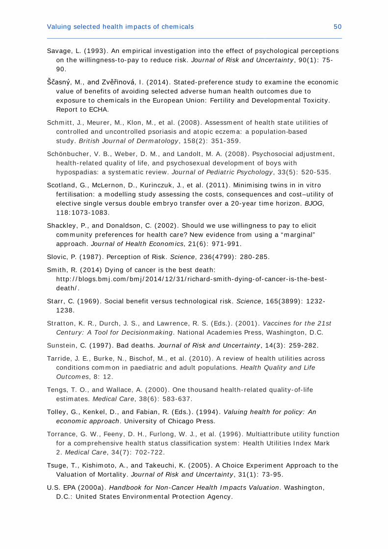
Valuing selected health impacts of chemicals 50
Savage, L. (1993). An empirical investigation into the effect of psychological perceptions on the willingness-to-pay to reduce risk. Journal of Risk and Uncertainty, 90(1): 75-90.
Ščasný, M., and Zvěřinová, I. (2014). Stated-preference study to examine the economic value of benefits of avoiding selected adverse human health outcomes due to exposure to chemicals in the European Union: Fertility and Developmental Toxicity. Report to ECHA.
Schmitt, J., Meurer, M., Klon, M., et al. (2008). Assessment of health state utilities of controlled and uncontrolled psoriasis and atopic eczema: a population‐based study. British Journal of Dermatology, 158(2): 351-359.
Schönbucher, V. B., Weber, D. M., and Landolt, M. A. (2008). Psychosocial adjustment, health-related quality of life, and psychosexual development of boys with hypospadias: a systematic review. Journal of Pediatric Psychology, 33(5): 520-535.
Scotland, G., McLernon, D., Kurinczuk, J., et al. (2011). Minimising twins in in vitro fertilisation: a modelling study assessing the costs, consequences and cost–utility of elective single versus double embryo transfer over a 20-year time horizon. BJOG, 118:1073-1083.
Shackley, P., and Donaldson, C. (2002). Should we use willingness to pay to elicit community preferences for health care? New evidence from using a “marginal” approach. Journal of Health Economics, 21(6): 971-991.
Slovic, P. (1987). Perception of Risk. Science, 236(4799): 280-285.
Smith, R. (2014) Dying of cancer is the best death: http://blogs.bmj.com/bmj/2014/12/31/richard-smith-dying-of-cancer-is-the-best-death/.
Starr, C. (1969). Social benefit versus technological risk. Science, 165(3899): 1232-1238.
Stratton, K. R., Durch, J. S., and Lawrence, R. S. (Eds.). (2001). Vaccines for the 21st Century: A Tool for Decisionmaking. National Academies Press, Washington, D.C.
Sunstein, C. (1997). Bad deaths. Journal of Risk and Uncertainty, 14(3): 259-282.
Tarride, J. E., Burke, N., Bischof, M., et al. (2010). A review of health utilities across conditions common in paediatric and adult populations. Health Quality and Life Outcomes, 8: 12.
Tengs, T. O., and Wallace, A. (2000). One thousand health-related quality-of-life estimates. Medical Care, 38(6): 583-637.
Tolley, G., Kenkel, D., and Fabian, R. (Eds.). (1994). Valuing health for policy: An economic approach. University of Chicago Press.
Torrance, G. W., Feeny, D. H., Furlong, W. J., et al. (1996). Multiattribute utility function for a comprehensive health status classification system: Health Utilities Index Mark 2. Medical Care, 34(7): 702-722.
Tsuge, T., Kishimoto, A., and Takeuchi, K. (2005). A Choice Experiment Approach to the Valuation of Mortality. Journal of Risk and Uncertainty, 31(1): 73-95.
U.S. EPA (2000a). Handbook for Non-Cancer Health Impacts Valuation. Washington, D.C.: United States Environmental Protection Agency.
Valuing selected health impacts of chemicals 51
U.S. EPA (2000b). Guidelines for Preparing Economic Analyses. EPA-R-00-003. Retrieved from http://yosemite.epa.gov/ee/epa/eerm.nsf/vwAN/EE-0568-50.pdf/$file/EE-0568-50.pdf
U.S. EPA (2013). America’s Children and the Environment (Third Edition). Washington, D.C.: United States Environmental Protection Agency.
Van den Akker-van Marke, M. E., Kamphuis, M., van Gameren-Oosterom, H. B., et al. (2013). Management of Undescended Testis A Decision Analysis. Medical Decision Making, 33(7): 906-919.
Van Houtven, G., and Smith, V. K. (1999). Willingness to Pay for Reductions in Infertility Risks: A Contingent Valuation Study. In Shi-Ling Hsu (Ed.), Valuing Health for Environmental Policy with Special Emphasis on Children's Health Protection, Proceedings of the Second Workshop in the Environmental Policy and Economics Workshop Series. Silver Spring, Maryland, March 24-25.
Van Houtven, G., Sullivan, M. B., and Dockins, C. (2008). Cancer premiums and latency effects: A risk tradeoff approach for valuing reductions in fatal cancer risks. Journal of Risk and Uncertainty, 36(2): 179-199.
Von Stackelberg, K., and Hammitt, J. K. (2009). Use of Contingent Valuation to Elicit Willingness-to-Pay for the Benefits of Developmental Health Risk Reductions. Environmental and Resource Economics, 43(1): 45-61.
Wehby, G. L., Ohsfeldt, R. L., and Murray, J. C. (2006). Health professionals' assessment of health-related quality of life values for oral clefting by age using a visual analogue scale method. The Cleft palate-craniofacial journal, 43(4): 383-391.
Wigle, D. T., Arbuckle, T. E., Turner, M. C., et al. (2008). Epidemiologic Evidence of Relationships Between Reproductive and Child Health Outcomes and Environmental Chemical Contaminants. Journal of Toxicology and Environmental Health – Part B, 11(5-6): 373–517.
Wooldridge, J. (2010). Econometric Analysis of Cross Section and Panel Data, 2nd ed., MIT Press, Cambridge, MA.
Yang, Y., Brazier, J., & Longworth, L. (2014). EQ-5D in skin conditions: an assessment of validity and responsiveness. European Journal of Health Economics, 16(9): 1-13.
Zug, K. A., Littenberg, B., Baughman, R.D., et al. (1995). Assessing the preferences of patients with psoriasis: a quantitative, utility approach. Archives of Dermatology, 131(5): 561-568.

EUROPEAN CHEMICALS AGENCY ANNANKATU 18, P.O. BOX 400, FI-00121 HELSINKI, FINLAND ECHA.EUROPA.EU
ED-A
H-15-001-EN
-N – D
oI: 10.2823/958237 – ISBN
: 978-92-9247-610-6 – ISSN
: 1831-7340