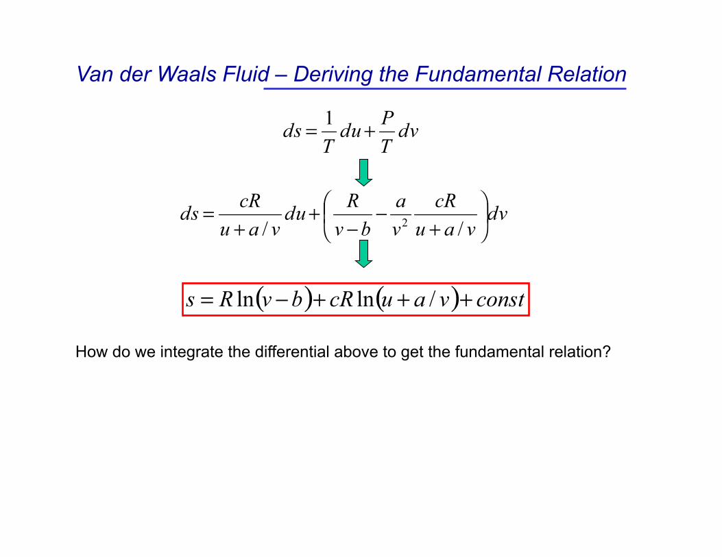
Van der Waals Fluid – Deriving the Fundamental Relation

How do we integrate the differential above to get the fundamental relation?

ds = cRu + a / v

du + Rv − b

−av2

cRu + a / v

⎛⎝⎜

⎞⎠⎟dv

Naïve approach: term-by-term “integration”:

After integration: - Wrong answer! This is because we treated variables as constants

Pitfalls of Integration of Functions of Multiple Variables

Pitfalls of Integration of Functions of Multiple Variables

ds = cRu + a / v

du + Rv − b

−av2

cRu + a / v

⎛⎝⎜

⎞⎠⎟dv

The correct way of integrating ds (note that although it works for the particular example of Van der Waals fluid, it is not generally applicable):

Now we have functions of the same arguments as differentials. Now integration is legitimate:

General Method of Integration

Problem: We have a differential form:

We also know that this form is an exact differential of a function s(u,v):

where

We can do “partial” integration of a differential equation above (assuming v is constant):

Note that the “constant” of integration must depend on v for the above procedure to be correct

General Method of Integration

4. Integrating both sides with respect to v, we obtain C(v)

1. “Partial” integration in u

2. Partial derivative in v

3. Substitution of N(u,v) for

The procedure above looks like a case of circular logic, but it always works

Ste

p 5

Sub

stitu

te C

(v)

General Method of Integration Applied to VdW Fluid

Let us apply the 5-step algorithm described above to the case of VdW fluid

1. “Partial” integration in u ( )

General Method of Integration Applied to VdW Fluid

2. Partial derivative in v

3. Substitution of N(u,v) for

General Method of Integration Applied to VdW Fluid

4. Integration of both sides with respect to v, we obtain C(v)

5. Substitution of C(v) back into the expression for s(u,v)

Rubber Band or Polymer

Let us chose the extensive coordinates of the system:

-  Internal energy U, is always a coordinate -  Length of the rubber band L

wall Tension force Γ

L

If we are not going to bend or twist the rubber band, we have enough coordinates to find the equilibrium state of the rubber band.

The fundamental relation will have a form: S(U,L)

rubber band

This example will show spectacular macroscopic manifestations of entropy – elasticity of an ideal rubber band is not due to “elastic energy” but is due to entropy!

Experimental observations:

1. Energy of the rubber band in equilibrium with the environment is independent of the length of the rubber band and is proportional to temperature:

where L0 is the equilibrium length (constant)

Rubber band or Polymer

2. Tension Γ is proportional to change in length:

- second experimental “equation of state”

- first experimental “equation of state”

Hooke’s law

3. Tension increases with increasing T for fixed length L.

The differential form of the fundamental relation is:

Since mixed second partial derivatives of S must be equal:

Rubber band or Polymer

Rubber band or Polymer

where B is a constant

Differentiability condition: Equations of state:

Rubber band or Polymer

Now we can substitute the equations of state into the differential for dS:

Integrating, we obtain:

We see that entropy decreases with increasing length of the rubber band (polymer chain). Therefore, the tendency of the rubber band to shrink is driven not by minimizing elastic energy (in our model there is no elastic energy) but by maximizing entropy

Polymer : microscopic model

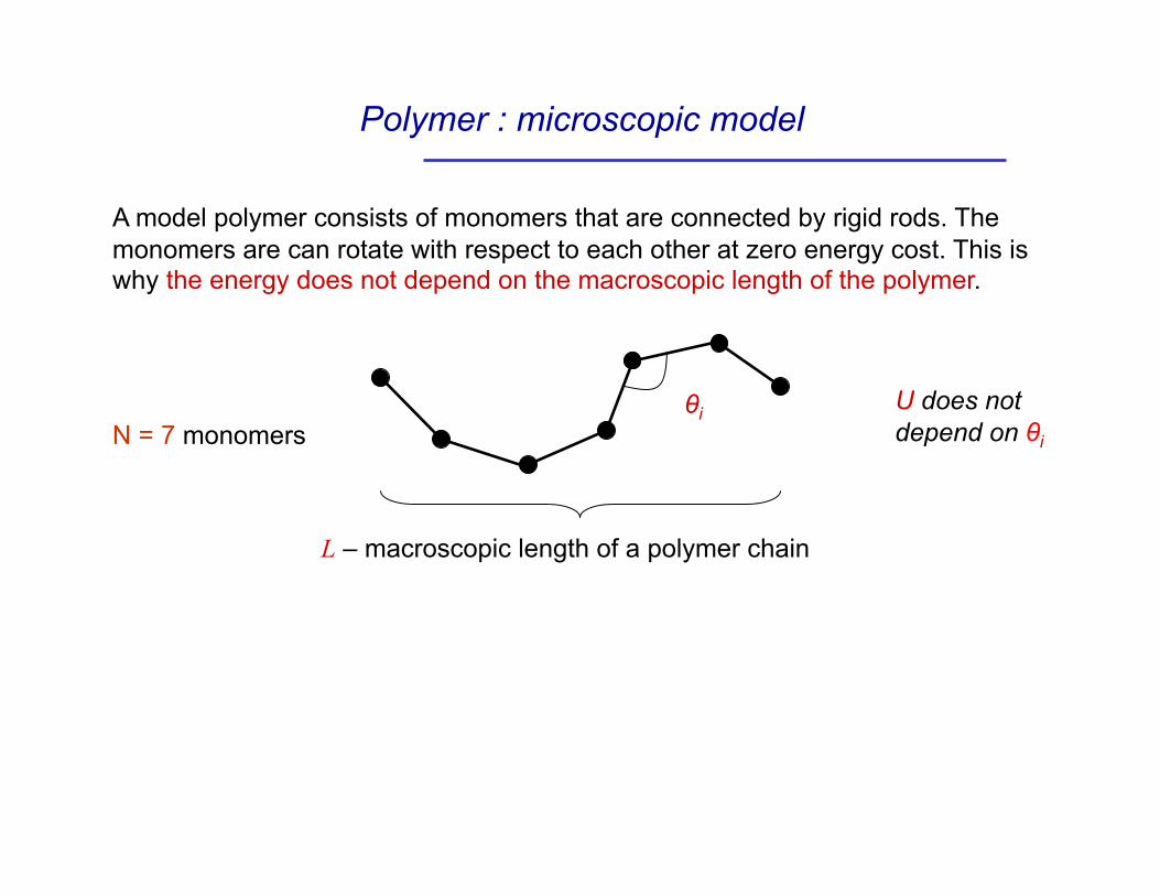
A model polymer consists of monomers that are connected by rigid rods. The monomers are can rotate with respect to each other at zero energy cost. This is why the energy does not depend on the macroscopic length of the polymer.

L – macroscopic length of a polymer chain

N = 7 monomers θi U does not

depend on θi

Polymer : microscopic model

We will examine a toy model of 2D polymer where monomers sit on a square lattice

N = 7

L = 4

Number of monomers, N, is fixed

Polymer length, L, is not constrained

Polymer: microscopic model

L = 6 Single microstate Ω = 1 S ~ ln(Ω)=0

Straight chain L = 4

Single kink

Number of microstates (assuming monomers cannot occupy the same volume): Ω = 8+6+4+2 ? S ~ ln(Ω) > 0

The number of microstates rises dramatically with decreasing length, so the entropy increases with decreasing length. State with L = 0 has the highest entropy.

These states have the same energy