PNNL-23381

Prepared for the U.S. Department of Energy under Contract DE-AC05-76RL01830

Vapor Intrusion Estimation Tool for Unsaturated-Zone Contaminant Sources CD Johnson MJ Truex KC Carroll M Oostrom AK Rice May 2014

PNNL-23381

Vapor Intrusion Estimation Tool for Unsaturated-Zone Contaminant Sources

CD Johnson1

MJ Truex1

KC Carroll2

M Oostrom1

AK Rice3

May 2014

1 Pacific Northwest National Laboratory

2 New Mexico State University

3 Colorado School of Mines

Prepared for

the U.S. Department of Energy

under Contract DE-AC05-76RL01830

Pacific Northwest National Laboratory

Richland, Washington 99354

iii

Executive Summary

This document presents a tool for estimating vapor intrusion into buildings resulting from unsaturated

(vadose) zone contaminant sources. The tool builds on, and is related to, guidance for evaluation of soil

vapor extraction (SVE) performance. The spreadsheet tool uses a quantitative estimation approach that

incorporates vadose zone source strength and location, vadose zone transport, and a model for estimating

movement of soil gas vapor contamination into buildings. The tool may be appropriate for a broad range

of site conditions. However, the user needs to consider the underlying assumptions used in the estimation

process when applying the tool. In some cases, vapor intrusion from groundwater plumes downgradient

of vadose zone source areas is important. The tool described here is focused on the vadose zone source

and is not configured to address vapors from downgradient groundwater plumes.

SVE is a prevalent remediation approach for volatile contaminants in the vadose zone. A diminishing

rate of contaminant extraction over time is typically observed due to 1) diminishing contaminant mass,

and/or 2) slow rates of removal for contamination in low-permeability zones. After a SVE system begins

to show indications of diminishing contaminant removal rate, SVE performance needs to be evaluated to

determine whether the system should be optimized, terminated, or transitioned to another technology to

replace or augment SVE. For many sites, part of this evaluation will include consideration of vapor

intrusion and quantifying the amount of source remediation necessary to meet vapor intrusion protection

goals.

The tool described here incorporates the results of three-dimensional multiphase transport simulations

predicting the concentration distribution from a vadose zone source. A large number of simulations were

conducted to develop a data set that can be queried based on the specific configuration of the user’s site.

If the user’s site configuration does not exactly match one of the existing simulation configurations,

interpolation is used to generate an appropriate vapor concentration estimate. With this approach, the

user has access to results from transport simulations without expending the time and effort to conduct

simulations themselves. This tool configuration also enables the user to rapidly conduct multiple

evaluations using variations in input parameters, thereby gaining insight into the sensitivity of the results

to variations in these parameters.

v

Acknowledgments

Funding for this work was provided by the Department of Defense Environmental Security Technology

Certification Program (ESTCP) under project number ER-201125. The Pacific Northwest National

Laboratory is operated by Battelle Memorial Institute for the U.S. Department of Energy under Contract

DE-AC05-76RL01830.

vii

Contents

Executive Summary .............................................................................................................................. iii

Acknowledgments ................................................................................................................................. v

1.0 Introduction .................................................................................................................................. 1

2.0 Calculational Steps ....................................................................................................................... 3

2.1 Compile Inputs for the Conceptual Site Model Framework ................................................ 4

2.2 Interpolation from Pre-Modeled Scenario Results for Nonlinear Variables ........................ 8

2.3 Scaling for Linear Variables ................................................................................................ 9

2.4 Estimation of Vapor Intrusion .............................................................................................. 11

2.5 Limitations and Assumptions ............................................................................................... 12

3.0 Example Calculation ..................................................................................................................... 15

4.0 VIETUS User Guide ..................................................................................................................... 21

4.1 System Requirements ........................................................................................................... 21

4.2 Installing and Starting VIETUS ........................................................................................... 21

4.3 Description of the VIETUS Workbook ................................................................................ 22

4.4 Using the Software ............................................................................................................... 25

5.0 References .................................................................................................................................... 27

viii

Figures

1 Conceptual framework for estimating the impact of a vadose zone contaminant source on

soil gas concentrations and vapor intrusion into a building .......................................................... 3

2 Flow chart of the steps involved in the process for estimating soil gas contaminant

concentration and building contaminant concentration due to vapor intrusion ............................ 4

3 Depiction of the permissible range for the gravimetric soil moisture content input parameter,

the corresponding values of residual saturation, and how the ranges are reconciled at the

lower and upper limits .................................................................................................................. 6

4 Example of the spatial interpolation from numerical grid cell centers to the location of

interest within the bounds of those cell centers ............................................................................ 16

5 View of the primary data on the “HLC” worksheet of the VIETUS workbook ........................... 22

6 Groupings of worksheet cells into blocks for input parameters, intermediate calculations, and

results ............................................................................................................................................ 23

7 View of the “VIETUS” worksheet, showing details of the input parameters, intermediate

calculations, results, and reference information ............................................................................ 24

Tables

1 Parameters defining source and transport site characteristics used in the estimation of soil

gas concentration .......................................................................................................................... 5

2 User input parameters defining vapor intrusion characteristics used in the estimation of the

building gas concentration ............................................................................................................ 7

3 Categorization of pairs of VZT and STR values to assist in data organization .............................. 9

4 Tabulated correlation coefficients for calculating vapor pressure and solubility of

contaminants of interest ................................................................................................................ 10

5 Tabulated correlation coefficients for calculating the gas diffusion coefficient for

contaminants of interest ................................................................................................................ 12

6 User input for the scenario variants applied in the example calculations for estimation of the

soil gas concentrations and vapor intrusion .................................................................................. 15

7 Parameter values for the example cases that are used in the second phase of interpolation ......... 16

8 Sequential interpolation to determine Cgu for the Cases A and B of the example ........................ 17

1

1.0 Introduction

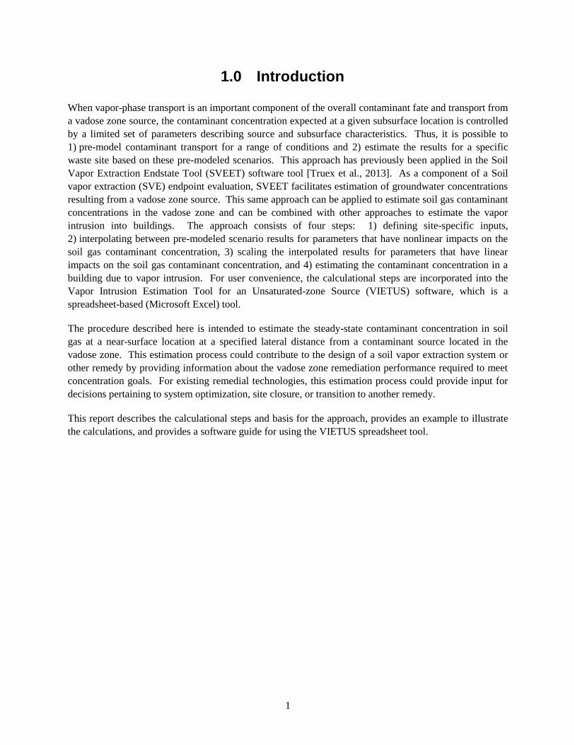
When vapor-phase transport is an important component of the overall contaminant fate and transport from

a vadose zone source, the contaminant concentration expected at a given subsurface location is controlled

by a limited set of parameters describing source and subsurface characteristics. Thus, it is possible to

1) pre-model contaminant transport for a range of conditions and 2) estimate the results for a specific

waste site based on these pre-modeled scenarios. This approach has previously been applied in the Soil

Vapor Extraction Endstate Tool (SVEET) software tool [Truex et al., 2013]. As a component of a Soil

vapor extraction (SVE) endpoint evaluation, SVEET facilitates estimation of groundwater concentrations

resulting from a vadose zone source. This same approach can be applied to estimate soil gas contaminant

concentrations in the vadose zone and can be combined with other approaches to estimate the vapor

intrusion into buildings. The approach consists of four steps: 1) defining site-specific inputs,

2) interpolating between pre-modeled scenario results for parameters that have nonlinear impacts on the

soil gas contaminant concentration, 3) scaling the interpolated results for parameters that have linear

impacts on the soil gas contaminant concentration, and 4) estimating the contaminant concentration in a

building due to vapor intrusion. For user convenience, the calculational steps are incorporated into the

Vapor Intrusion Estimation Tool for an Unsaturated-zone Source (VIETUS) software, which is a

spreadsheet-based (Microsoft Excel) tool.

The procedure described here is intended to estimate the steady-state contaminant concentration in soil

gas at a near-surface location at a specified lateral distance from a contaminant source located in the

vadose zone. This estimation process could contribute to the design of a soil vapor extraction system or

other remedy by providing information about the vadose zone remediation performance required to meet

concentration goals. For existing remedial technologies, this estimation process could provide input for

decisions pertaining to system optimization, site closure, or transition to another remedy.

This report describes the calculational steps and basis for the approach, provides an example to illustrate

the calculations, and provides a software guide for using the VIETUS spreadsheet tool.

3

2.0 Calculational Steps

The approach for estimating a soil gas contaminant concentration in the vadose zone and the

corresponding gas concentration in a building due to vapor intrusion is based on a generalized conceptual

site model and is comprised of several calculational steps.

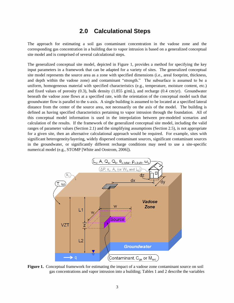
The generalized conceptual site model, depicted in Figure 1, provides a method for specifying the key

input parameters in a framework that can be adapted for a variety of sites. The generalized conceptual

site model represents the source area as a zone with specified dimensions (i.e., areal footprint, thickness,

and depth within the vadose zone) and contaminant “strength.” The subsurface is assumed to be a

uniform, homogeneous material with specified characteristics (e.g., temperature, moisture content, etc.)

and fixed values of porosity (0.3), bulk density (1.855 g/mL), and recharge (0.4 cm/yr). Groundwater

beneath the vadose zone flows at a specified rate, with the orientation of the conceptual model such that

groundwater flow is parallel to the x-axis. A single building is assumed to be located at a specified lateral

distance from the center of the source area, not necessarily on the axis of the model. The building is

defined as having specified characteristics pertaining to vapor intrusion through the foundation. All of

this conceptual model information is used in the interpolation between pre-modeled scenarios and

calculation of the results. If the framework of the generalized conceptual site model, including the valid

ranges of parameter values (Section 2.1) and the simplifying assumptions (Section 2.5), is not appropriate

for a given site, then an alternative calculational approach would be required. For example, sites with

significant heterogeneity/layering, widely dispersed contaminant sources, significant contaminant sources

in the groundwater, or significantly different recharge conditions may need to use a site-specific

numerical model (e.g., STOMP [White and Oostrom, 2006]).

Figure 1. Conceptual framework for estimating the impact of a vadose zone contaminant source on soil

gas concentrations and vapor intrusion into a building; Tables 1 and 2 describe the variables

4

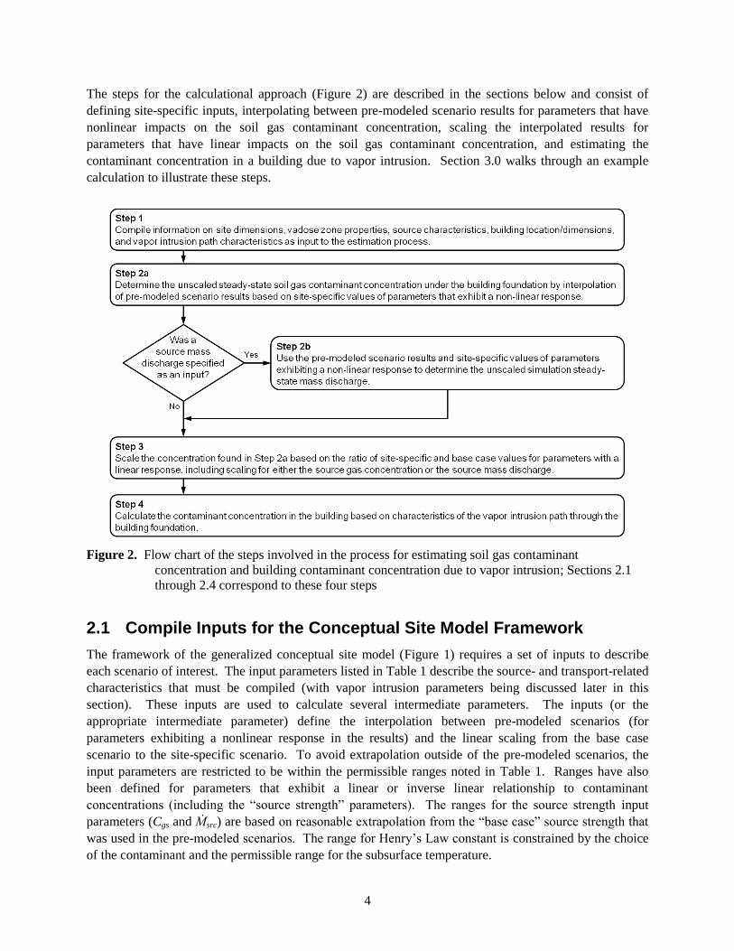
The steps for the calculational approach (Figure 2) are described in the sections below and consist of

defining site-specific inputs, interpolating between pre-modeled scenario results for parameters that have

nonlinear impacts on the soil gas contaminant concentration, scaling the interpolated results for

parameters that have linear impacts on the soil gas contaminant concentration, and estimating the

contaminant concentration in a building due to vapor intrusion. Section 3.0 walks through an example

calculation to illustrate these steps.

Figure 2. Flow chart of the steps involved in the process for estimating soil gas contaminant

concentration and building contaminant concentration due to vapor intrusion; Sections 2.1

through 2.4 correspond to these four steps

2.1 Compile Inputs for the Conceptual Site Model Framework

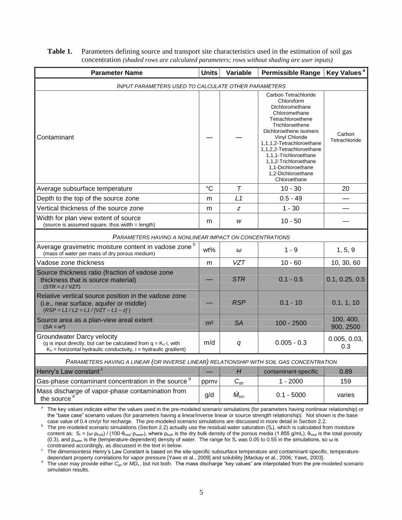
The framework of the generalized conceptual site model (Figure 1) requires a set of inputs to describe

each scenario of interest. The input parameters listed in Table 1 describe the source- and transport-related

characteristics that must be compiled (with vapor intrusion parameters being discussed later in this

section). These inputs are used to calculate several intermediate parameters. The inputs (or the

appropriate intermediate parameter) define the interpolation between pre-modeled scenarios (for

parameters exhibiting a nonlinear response in the results) and the linear scaling from the base case

scenario to the site-specific scenario. To avoid extrapolation outside of the pre-modeled scenarios, the

input parameters are restricted to be within the permissible ranges noted in Table 1. Ranges have also

been defined for parameters that exhibit a linear or inverse linear relationship to contaminant

concentrations (including the “source strength” parameters). The ranges for the source strength input

parameters (Cgs and Ṁsrc) are based on reasonable extrapolation from the “base case” source strength that

was used in the pre-modeled scenarios. The range for Henry’s Law constant is constrained by the choice

of the contaminant and the permissible range for the subsurface temperature.

5

Table 1. Parameters defining source and transport site characteristics used in the estimation of soil gas

concentration (shaded rows are calculated parameters; rows without shading are user inputs)

Parameter Name Units Variable Permissible Range Key Values a

INPUT PARAMETERS USED TO CALCULATE OTHER PARAMETERS

Contaminant — —

Carbon Tetrachloride Chloroform

Dichloromethane Chloromethane

Tetrachloroethene Trichloroethene

Dichloroethene isomers Vinyl Chloride

1,1,1,2-Tetrachloroethane 1,1,2,2-Tetrachloroethane

1,1,1-Trichloroethane 1,1,2-Trichloroethane 1,1-Dichloroethane 1,2-Dichloroethane

Chloroethane

Carbon Tetrachloride

Average subsurface temperature °C T 10 - 30 20

Depth to the top of the source zone m L1 0.5 - 49 —

Vertical thickness of the source zone m z 1 - 30 —

Width for plan view extent of source (source is assumed square, thus width = length)

m w 10 - 50 —

PARAMETERS HAVING A NONLINEAR IMPACT ON CONCENTRATIONS

Average gravimetric moisture content in vadose zone b

(mass of water per mass of dry porous medium)

wt% ω 1 - 9 1, 5, 9

Vadose zone thickness m VZT 10 - 60 10, 30, 60

Source thickness ratio (fraction of vadose zone thickness that is source material)

(STR = z / VZT) — STR 0.1 - 0.5 0.1, 0.25, 0.5

Relative vertical source position in the vadose zone (i.e., near surface, aquifer or middle)

(RSP = L1 / L2 = L1 / [VZT – L1 – z] )

— RSP 0.1 - 10 0.1, 1, 10

Source area as a plan-view areal extent (SA = w²)

m² SA 100 - 2500 100, 400, 900, 2500

Groundwater Darcy velocity (q is input directly, but can be calculated from q = Kh·i, with

Kh = horizontal hydraulic conductivity, i = hydraulic gradient) m/d q 0.005 - 0.3

0.005, 0.03, 0.3

PARAMETERS HAVING A LINEAR (OR INVERSE LINEAR) RELATIONSHIP WITH SOIL GAS CONCENTRATION

Henry’s Law constant c — H contaminant-specific 0.89

Gas-phase contaminant concentration in the source d ppmv Cgs 1 - 2000 159

Mass discharge of vapor-phase contamination from the source

d

g/d Ṁsrc 0.1 - 5000 varies

a The key values indicate either the values used in the pre-modeled scenario simulations (for parameters having nonlinear relationship) or

the “base case” scenario values (for parameters having a linear/inverse linear or source strength relationship). Not shown is the base case value of 0.4 cm/yr for recharge. The pre-modeled scenario simulations are discussed in more detail in Section 2.2.

b The pre-modeled scenario simulations (Section 2.2) actually use the residual water saturation (Sr), which is calculated from moisture

content as: Sr = (ω·ρbulk) / (100·θtotal·ρwater), where ρbulk is the dry bulk density of the porous media (1.855 g/mL), θtotal is the total porosity (0.3), and ρwater is the (temperature-dependent) density of water. The range for Sr was 0.05 to 0.55 in the simulations, so ω is constrained accordingly, as discussed in the text in below.

c The dimensionless Henry’s Law Constant is based on the site-specific subsurface temperature and contaminant-specific, temperature-

dependant property correlations for vapor pressure [Yaws et al., 2009] and solubility [Mackay et al., 2006; Yaws, 2003]. d The user may provide either Cgs or MDs , but not both. The mass discharge “key values” are interpolated from the pre-modeled scenario

simulation results.

6

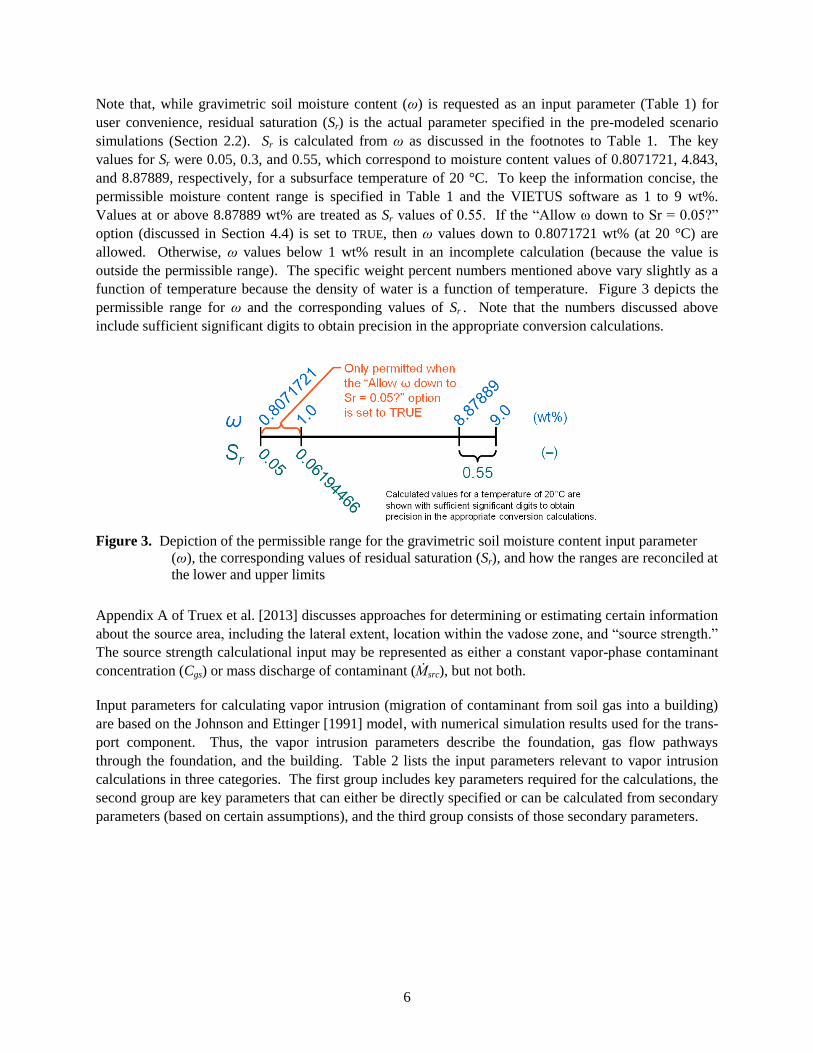
Note that, while gravimetric soil moisture content (ω) is requested as an input parameter (Table 1) for

user convenience, residual saturation (Sr) is the actual parameter specified in the pre-modeled scenario

simulations (Section 2.2). Sr is calculated from ω as discussed in the footnotes to Table 1. The key

values for Sr were 0.05, 0.3, and 0.55, which correspond to moisture content values of 0.8071721, 4.843,

and 8.87889, respectively, for a subsurface temperature of 20 °C. To keep the information concise, the

permissible moisture content range is specified in Table 1 and the VIETUS software as 1 to 9 wt%.

Values at or above 8.87889 wt% are treated as Sr values of 0.55. If the “Allow ω down to Sr = 0.05?”

option (discussed in Section 4.4) is set to TRUE, then ω values down to 0.8071721 wt% (at 20 °C) are

allowed. Otherwise, ω values below 1 wt% result in an incomplete calculation (because the value is

outside the permissible range). The specific weight percent numbers mentioned above vary slightly as a

function of temperature because the density of water is a function of temperature. Figure 3 depicts the

permissible range for ω and the corresponding values of Sr . Note that the numbers discussed above

include sufficient significant digits to obtain precision in the appropriate conversion calculations.

Figure 3. Depiction of the permissible range for the gravimetric soil moisture content input parameter

(ω), the corresponding values of residual saturation (Sr), and how the ranges are reconciled at

the lower and upper limits

Appendix A of Truex et al. [2013] discusses approaches for determining or estimating certain information

about the source area, including the lateral extent, location within the vadose zone, and “source strength.”

The source strength calculational input may be represented as either a constant vapor-phase contaminant

concentration (Cgs) or mass discharge of contaminant (Ṁsrc), but not both.

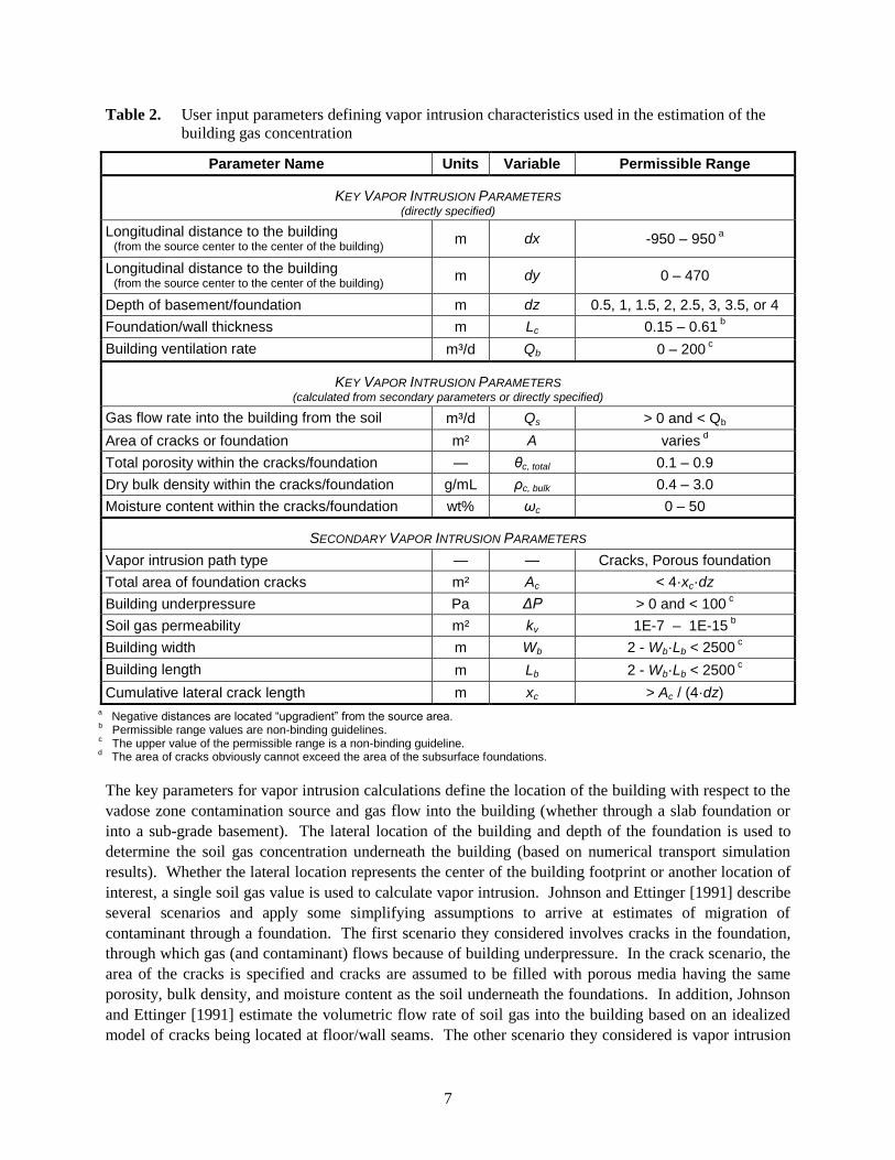
Input parameters for calculating vapor intrusion (migration of contaminant from soil gas into a building)

are based on the Johnson and Ettinger [1991] model, with numerical simulation results used for the trans-

port component. Thus, the vapor intrusion parameters describe the foundation, gas flow pathways

through the foundation, and the building. Table 2 lists the input parameters relevant to vapor intrusion

calculations in three categories. The first group includes key parameters required for the calculations, the

second group are key parameters that can either be directly specified or can be calculated from secondary

parameters (based on certain assumptions), and the third group consists of those secondary parameters.

7

Table 2. User input parameters defining vapor intrusion characteristics used in the estimation of the

building gas concentration

Parameter Name Units Variable Permissible Range

KEY VAPOR INTRUSION PARAMETERS (directly specified)

Longitudinal distance to the building (from the source center to the center of the building) m dx -950 – 950

a

Longitudinal distance to the building (from the source center to the center of the building) m dy 0 – 470

Depth of basement/foundation m dz 0.5, 1, 1.5, 2, 2.5, 3, 3.5, or 4

Foundation/wall thickness m Lc 0.15 – 0.61 b

Building ventilation rate m³/d Qb 0 – 200 c

KEY VAPOR INTRUSION PARAMETERS (calculated from secondary parameters or directly specified)

Gas flow rate into the building from the soil m³/d Qs > 0 and < Qb

Area of cracks or foundation m² A varies d

Total porosity within the cracks/foundation — θc, total 0.1 – 0.9

Dry bulk density within the cracks/foundation g/mL ρc, bulk 0.4 – 3.0

Moisture content within the cracks/foundation wt% ωc 0 – 50

SECONDARY VAPOR INTRUSION PARAMETERS

Vapor intrusion path type — — Cracks, Porous foundation

Total area of foundation cracks m² Ac < 4·xc·dz

Building underpressure Pa ΔP > 0 and < 100 c

Soil gas permeability m² kv 1E-7 – 1E-15 b

Building width m Wb 2 - Wb·Lb < 2500 c

Building length m Lb 2 - Wb·Lb < 2500 c

Cumulative lateral crack length m xc > Ac / (4·dz) a Negative distances are located “upgradient” from the source area.

b Permissible range values are non-binding guidelines.

c The upper value of the permissible range is a non-binding guideline.

d The area of cracks obviously cannot exceed the area of the subsurface foundations.

The key parameters for vapor intrusion calculations define the location of the building with respect to the

vadose zone contamination source and gas flow into the building (whether through a slab foundation or

into a sub-grade basement). The lateral location of the building and depth of the foundation is used to

determine the soil gas concentration underneath the building (based on numerical transport simulation

results). Whether the lateral location represents the center of the building footprint or another location of

interest, a single soil gas value is used to calculate vapor intrusion. Johnson and Ettinger [1991] describe

several scenarios and apply some simplifying assumptions to arrive at estimates of migration of

contaminant through a foundation. The first scenario they considered involves cracks in the foundation,

through which gas (and contaminant) flows because of building underpressure. In the crack scenario, the

area of the cracks is specified and cracks are assumed to be filled with porous media having the same

porosity, bulk density, and moisture content as the soil underneath the foundations. In addition, Johnson

and Ettinger [1991] estimate the volumetric flow rate of soil gas into the building based on an idealized

model of cracks being located at floor/wall seams. The other scenario they considered is vapor intrusion

8

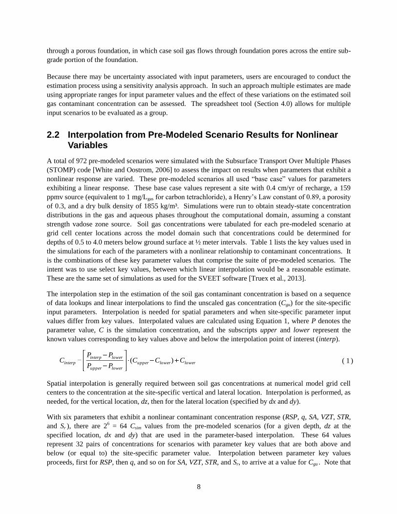
through a porous foundation, in which case soil gas flows through foundation pores across the entire sub-

grade portion of the foundation.

Because there may be uncertainty associated with input parameters, users are encouraged to conduct the

estimation process using a sensitivity analysis approach. In such an approach multiple estimates are made

using appropriate ranges for input parameter values and the effect of these variations on the estimated soil

gas contaminant concentration can be assessed. The spreadsheet tool (Section 4.0) allows for multiple

input scenarios to be evaluated as a group.

2.2 Interpolation from Pre-Modeled Scenario Results for Nonlinear Variables

A total of 972 pre-modeled scenarios were simulated with the Subsurface Transport Over Multiple Phases

(STOMP) code [White and Oostrom, 2006] to assess the impact on results when parameters that exhibit a

nonlinear response are varied. These pre-modeled scenarios all used “base case” values for parameters

exhibiting a linear response. These base case values represent a site with 0.4 cm/yr of recharge, a 159

ppmv source (equivalent to 1 mg/Lgas for carbon tetrachloride), a Henry’s Law constant of 0.89, a porosity

of 0.3, and a dry bulk density of 1855 kg/m³. Simulations were run to obtain steady-state concentration

distributions in the gas and aqueous phases throughout the computational domain, assuming a constant

strength vadose zone source. Soil gas concentrations were tabulated for each pre-modeled scenario at

grid cell center locations across the model domain such that concentrations could be determined for

depths of 0.5 to 4.0 meters below ground surface at ½ meter intervals. Table 1 lists the key values used in

the simulations for each of the parameters with a nonlinear relationship to contaminant concentrations. It

is the combinations of these key parameter values that comprise the suite of pre-modeled scenarios. The

intent was to use select key values, between which linear interpolation would be a reasonable estimate.

These are the same set of simulations as used for the SVEET software [Truex et al., 2013].

The interpolation step in the estimation of the soil gas contaminant concentration is based on a sequence

of data lookups and linear interpolations to find the unscaled gas concentration (Cgu) for the site-specific

input parameters. Interpolation is needed for spatial parameters and when site-specific parameter input

values differ from key values. Interpolated values are calculated using Equation 1, where P denotes the

parameter value, C is the simulation concentration, and the subscripts upper and lower represent the

known values corresponding to key values above and below the interpolation point of interest (interp).

lowerlowerupper

lowerupper

lowerinterp

interp CCCPP

PPC )( ( 1 )

Spatial interpolation is generally required between soil gas concentrations at numerical model grid cell

centers to the concentration at the site-specific vertical and lateral location. Interpolation is performed, as

needed, for the vertical location, dz, then for the lateral location (specified by dx and dy).

With six parameters that exhibit a nonlinear contaminant concentration response (RSP, q, SA, VZT, STR,

and Sr ), there are 26 = 64 Csim values from the pre-modeled scenarios (for a given depth, dz at the

specified location, dx and dy) that are used in the parameter-based interpolation. These 64 values

represent 32 pairs of concentrations for scenarios with parameter key values that are both above and

below (or equal to) the site-specific parameter value. Interpolation between parameter key values

proceeds, first for RSP, then q, and so on for SA, VZT, STR, and Sr, to arrive at a value for Cgu . Note that

9

Sr is the water saturation value converted from the ω moisture content value (as discussed in the footnotes

to Table 1).

If the source strength input parameter was provided as a Ṁsrc value (i.e., not a Cgs value), then a second

sequence of lookups/interpolations (in the same order of RSP, q, SA, VZT, STR, and Sr) is performed to

determine the simulated contaminant mass discharge (Ṁsim) corresponding to the input site parameters.

This Ṁsim value is needed as a linear scaling factor. The process for obtaining the interpolated Ṁsim mass

discharge value is the same as for Cgu , except that spatial interpolation does not apply.

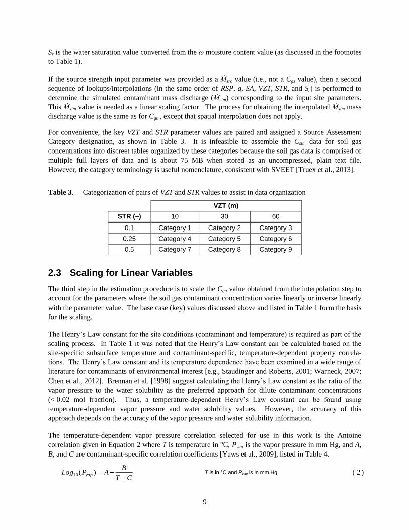
For convenience, the key VZT and STR parameter values are paired and assigned a Source Assessment

Category designation, as shown in Table 3. It is infeasible to assemble the Csim data for soil gas

concentrations into discreet tables organized by these categories because the soil gas data is comprised of

multiple full layers of data and is about 75 MB when stored as an uncompressed, plain text file.

However, the category terminology is useful nomenclature, consistent with SVEET [Truex et al., 2013].

Table 3. Categorization of pairs of VZT and STR values to assist in data organization

VZT (m)

STR (–) 10 30 60

0.1 Category 1 Category 2 Category 3

0.25 Category 4 Category 5 Category 6

0.5 Category 7 Category 8 Category 9

2.3 Scaling for Linear Variables

The third step in the estimation procedure is to scale the Cgu value obtained from the interpolation step to

account for the parameters where the soil gas contaminant concentration varies linearly or inverse linearly

with the parameter value. The base case (key) values discussed above and listed in Table 1 form the basis

for the scaling.

The Henry’s Law constant for the site conditions (contaminant and temperature) is required as part of the

scaling process. In Table 1 it was noted that the Henry’s Law constant can be calculated based on the

site-specific subsurface temperature and contaminant-specific, temperature-dependent property correla-

tions. The Henry’s Law constant and its temperature dependence have been examined in a wide range of

literature for contaminants of environmental interest [e.g., Staudinger and Roberts, 2001; Warneck, 2007;

Chen et al., 2012]. Brennan et al. [1998] suggest calculating the Henry’s Law constant as the ratio of the

vapor pressure to the water solubility as the preferred approach for dilute contaminant concentrations

(< 0.02 mol fraction). Thus, a temperature-dependent Henry’s Law constant can be found using

temperature-dependent vapor pressure and water solubility values. However, the accuracy of this

approach depends on the accuracy of the vapor pressure and water solubility information.

The temperature-dependent vapor pressure correlation selected for use in this work is the Antoine

correlation given in Equation 2 where T is temperature in °C, Pvap is the vapor pressure in mm Hg, and A,

B, and C are contaminant-specific correlation coefficients [Yaws et al., 2009], listed in Table 4.

CT

BAPLog vap )(10

T is in °C and Pvap is in mm Hg ( 2 )

10

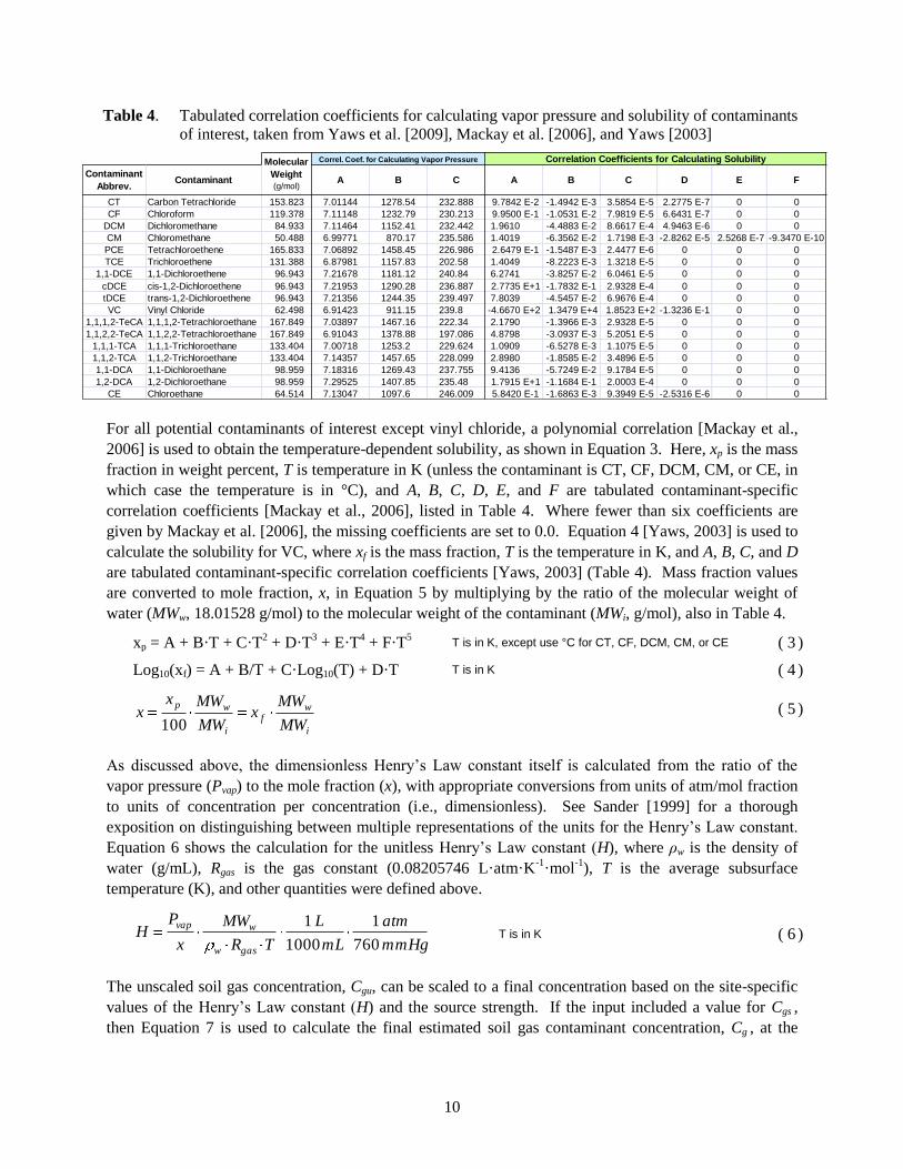
Table 4. Tabulated correlation coefficients for calculating vapor pressure and solubility of contaminants

of interest, taken from Yaws et al. [2009], Mackay et al. [2006], and Yaws [2003]

For all potential contaminants of interest except vinyl chloride, a polynomial correlation [Mackay et al.,

2006] is used to obtain the temperature-dependent solubility, as shown in Equation 3. Here, xp is the mass

fraction in weight percent, T is temperature in K (unless the contaminant is CT, CF, DCM, CM, or CE, in

which case the temperature is in °C), and A, B, C, D, E, and F are tabulated contaminant-specific

correlation coefficients [Mackay et al., 2006], listed in Table 4. Where fewer than six coefficients are

given by Mackay et al. [2006], the missing coefficients are set to 0.0. Equation 4 [Yaws, 2003] is used to

calculate the solubility for VC, where xf is the mass fraction, T is the temperature in K, and A, B, C, and D

are tabulated contaminant-specific correlation coefficients [Yaws, 2003] (Table 4). Mass fraction values

are converted to mole fraction, x, in Equation 5 by multiplying by the ratio of the molecular weight of

water (MWw, 18.01528 g/mol) to the molecular weight of the contaminant (MWi, g/mol), also in Table 4.

xp = A + B·T + C·T2 + D·T

3 + E·T

4 + F·T

5 T is in K, except use °C for CT, CF, DCM, CM, or CE ( 3 )

Log10(xf) = A + B/T + C·Log10(T) + D·T T is in K ( 4 )

i

wf

i

wp

MW

MWx

MW

MWxx

100 ( 5 )

As discussed above, the dimensionless Henry’s Law constant itself is calculated from the ratio of the

vapor pressure (Pvap) to the mole fraction (x), with appropriate conversions from units of atm/mol fraction

to units of concentration per concentration (i.e., dimensionless). See Sander [1999] for a thorough

exposition on distinguishing between multiple representations of the units for the Henry’s Law constant.

Equation 6 shows the calculation for the unitless Henry’s Law constant (H), where ρw is the density of

water (g/mL), Rgas is the gas constant (0.08205746 L·atm·K-1

·mol-1

), T is the average subsurface

temperature (K), and other quantities were defined above.

mmHg

atm

mL

L

TR

MW

x

PH

gasw

wvap

760

1

1000

1 T is in K ( 6 )

The unscaled soil gas concentration, Cgu, can be scaled to a final concentration based on the site-specific

values of the Henry’s Law constant (H) and the source strength. If the input included a value for Cgs ,

then Equation 7 is used to calculate the final estimated soil gas contaminant concentration, Cg , at the

Correl. Coef. for Calculating Vapor Pressure Correlation Coefficients for Calculating Solubility Correl. Coef. for Calculating Gas Diffusion Coef.

Contaminant

Abbrev.Contaminant A B C A B C D E F

CT Carbon Tetrachloride 153.823 7.01144 1278.54 232.888 9.7842 E-2 -1.4942 E-3 3.5854 E-5 2.2775 E-7 0 0

CF Chloroform 119.378 7.11148 1232.79 230.213 9.9500 E-1 -1.0531 E-2 7.9819 E-5 6.6431 E-7 0 0

DCM Dichloromethane 84.933 7.11464 1152.41 232.442 1.9610 -4.4883 E-2 8.6617 E-4 4.9463 E-6 0 0

CM Chloromethane 50.488 6.99771 870.17 235.586 1.4019 -6.3562 E-2 1.7198 E-3 -2.8262 E-5 2.5268 E-7 -9.3470 E-10

PCE Tetrachloroethene 165.833 7.06892 1458.45 226.986 2.6479 E-1 -1.5487 E-3 2.4477 E-6 0 0 0

TCE Trichloroethene 131.388 6.87981 1157.83 202.58 1.4049 -8.2223 E-3 1.3218 E-5 0 0 0

1,1-DCE 1,1-Dichloroethene 96.943 7.21678 1181.12 240.84 6.2741 -3.8257 E-2 6.0461 E-5 0 0 0

cDCE cis-1,2-Dichloroethene 96.943 7.21953 1290.28 236.887 2.7735 E+1 -1.7832 E-1 2.9328 E-4 0 0 0

tDCE trans-1,2-Dichloroethene 96.943 7.21356 1244.35 239.497 7.8039 -4.5457 E-2 6.9676 E-4 0 0 0

VC Vinyl Chloride 62.498 6.91423 911.15 239.8 -4.6670 E+2 1.3479 E+4 1.8523 E+2 -1.3236 E-1 0 0

1,1,1,2-TeCA 1,1,1,2-Tetrachloroethane 167.849 7.03897 1467.16 222.34 2.1790 -1.3966 E-3 2.9328 E-5 0 0 0

1,1,2,2-TeCA 1,1,2,2-Tetrachloroethane 167.849 6.91043 1378.88 197.086 4.8798 -3.0937 E-3 5.2051 E-5 0 0 0

1,1,1-TCA 1,1,1-Trichloroethane 133.404 7.00718 1253.2 229.624 1.0909 -6.5278 E-3 1.1075 E-5 0 0 0

1,1,2-TCA 1,1,2-Trichloroethane 133.404 7.14357 1457.65 228.099 2.8980 -1.8585 E-2 3.4896 E-5 0 0 0

1,1-DCA 1,1-Dichloroethane 98.959 7.18316 1269.43 237.755 9.4136 -5.7249 E-2 9.1784 E-5 0 0 0

1,2-DCA 1,2-Dichloroethane 98.959 7.29525 1407.85 235.48 1.7915 E+1 -1.1684 E-1 2.0003 E-4 0 0 0

CE Chloroethane 64.514 7.13047 1097.6 246.009 5.8420 E-1 -1.6863 E-3 9.3949 E-5 -2.5316 E-6 0 0

Molecular

Weight

(g/mol)

11

location directly below the building foundation. If the input included Ṁsrc , then Equation 8 is used to

calculate Cg .

0159

C

H

890CC

gs

gug.

. ( 7 )

sim

srcgug

M

M

H

890CC

. ( 8 )

2.4 Estimation of Vapor Intrusion

Vapor intrusion is calculated based on the approach described by Johnson and Ettinger [1991], with the

variation that the soil gas concentration underneath the building foundation, Cg , is determined from the

interpolation and scaling steps described above. Johnson and Ettinger specify equations for the entry rate

of contaminant into a building (in their equations 14 and 17). Rearranging their equations to solve for the

concentration in the building, Cb , results in Equation 9. This equation defines the key parameters that are

required as inputs (as listed in Table 2).

sb

c

csb

c

csgs

b

QQAD

LQQ

AD

LQCQ

C

exp

exp

( 9 )

The only parameter in Equation 9 that is not listed in Table 2 is the gas diffusion coefficient in porous

media (i.e., crack or foundation) for the contaminant of interest, Dc , which is calculated with Equation 10

using the same Millington-Quirk approach as taken by Johnson and Ettinger [1991]. Here, θc,g is the gas

porosity of the cracks/foundation, ρwater is the density of water at the subsurface temperature, and Da is the

diffusion coefficient in air (m²/day) for the contaminant of interest. The diffusion coefficient in air can be

calculated from Equation 11 using the tabulated contaminant-specific correlation coefficients listed in

Table 5 [Yaws, 2003].

2

totalc

water

bulkcc

totalca

2

totalc

gca

c

310

310

100D

DD

,

,

,

,

,

( 10 )

)/()( 22

a 10086400TCTBAD T is in K ( 11 )

12

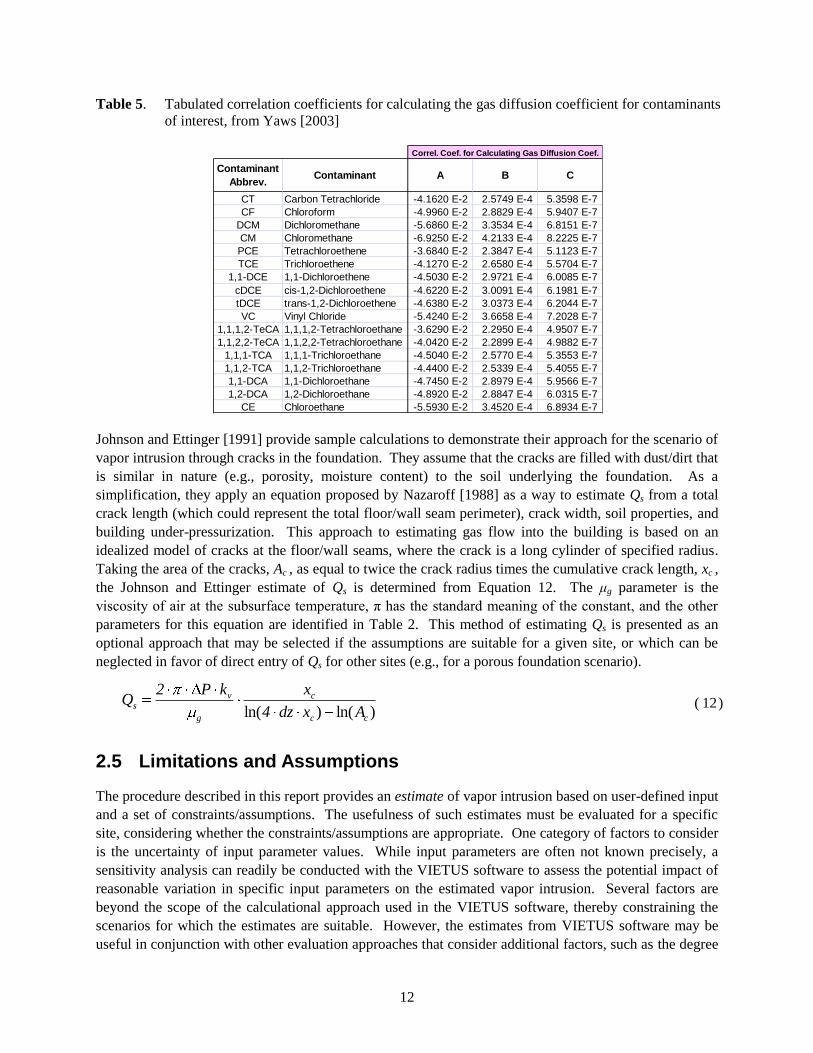
Table 5. Tabulated correlation coefficients for calculating the gas diffusion coefficient for contaminants

of interest, from Yaws [2003]

Johnson and Ettinger [1991] provide sample calculations to demonstrate their approach for the scenario of

vapor intrusion through cracks in the foundation. They assume that the cracks are filled with dust/dirt that

is similar in nature (e.g., porosity, moisture content) to the soil underlying the foundation. As a

simplification, they apply an equation proposed by Nazaroff [1988] as a way to estimate Qs from a total

crack length (which could represent the total floor/wall seam perimeter), crack width, soil properties, and

building under-pressurization. This approach to estimating gas flow into the building is based on an

idealized model of cracks at the floor/wall seams, where the crack is a long cylinder of specified radius.

Taking the area of the cracks, Ac , as equal to twice the crack radius times the cumulative crack length, xc ,

the Johnson and Ettinger estimate of Qs is determined from Equation 12. The μg parameter is the

viscosity of air at the subsurface temperature, π has the standard meaning of the constant, and the other

parameters for this equation are identified in Table 2. This method of estimating Qs is presented as an

optional approach that may be selected if the assumptions are suitable for a given site, or which can be

neglected in favor of direct entry of Qs for other sites (e.g., for a porous foundation scenario).

)ln()ln( cc

c

g

vs

Axdz4

xkP2Q ( 12 )

2.5 Limitations and Assumptions

The procedure described in this report provides an estimate of vapor intrusion based on user-defined input

and a set of constraints/assumptions. The usefulness of such estimates must be evaluated for a specific

site, considering whether the constraints/assumptions are appropriate. One category of factors to consider

is the uncertainty of input parameter values. While input parameters are often not known precisely, a

sensitivity analysis can readily be conducted with the VIETUS software to assess the potential impact of

reasonable variation in specific input parameters on the estimated vapor intrusion. Several factors are

beyond the scope of the calculational approach used in the VIETUS software, thereby constraining the

scenarios for which the estimates are suitable. However, the estimates from VIETUS software may be

useful in conjunction with other evaluation approaches that consider additional factors, such as the degree

Correl. Coef. for Calculating Gas Diffusion Coef.

Contaminant

Abbrev.Contaminant A B C

CT Carbon Tetrachloride -4.1620 E-2 2.5749 E-4 5.3598 E-7

CF Chloroform -4.9960 E-2 2.8829 E-4 5.9407 E-7

DCM Dichloromethane -5.6860 E-2 3.3534 E-4 6.8151 E-7

CM Chloromethane -6.9250 E-2 4.2133 E-4 8.2225 E-7

PCE Tetrachloroethene -3.6840 E-2 2.3847 E-4 5.1123 E-7

TCE Trichloroethene -4.1270 E-2 2.6580 E-4 5.5704 E-7

1,1-DCE 1,1-Dichloroethene -4.5030 E-2 2.9721 E-4 6.0085 E-7

cDCE cis-1,2-Dichloroethene -4.6220 E-2 3.0091 E-4 6.1981 E-7

tDCE trans-1,2-Dichloroethene -4.6380 E-2 3.0373 E-4 6.2044 E-7

VC Vinyl Chloride -5.4240 E-2 3.6658 E-4 7.2028 E-7

1,1,1,2-TeCA 1,1,1,2-Tetrachloroethane -3.6290 E-2 2.2950 E-4 4.9507 E-7

1,1,2,2-TeCA 1,1,2,2-Tetrachloroethane -4.0420 E-2 2.2899 E-4 4.9882 E-7

1,1,1-TCA 1,1,1-Trichloroethane -4.5040 E-2 2.5770 E-4 5.3553 E-7

1,1,2-TCA 1,1,2-Trichloroethane -4.4400 E-2 2.5339 E-4 5.4055 E-7

1,1-DCA 1,1-Dichloroethane -4.7450 E-2 2.8979 E-4 5.9566 E-7

1,2-DCA 1,2-Dichloroethane -4.8920 E-2 2.8847 E-4 6.0315 E-7

CE Chloroethane -5.5930 E-2 3.4520 E-4 6.8934 E-7

13

of source depletion over time, adsorption, biological transformation, other physical attenuation

mechanisms, multiple sources, sources in the groundwater, and variation in recharge/infiltration through

the vadose zone source. In addition to constraints of the calculational approach, the appropriateness of

simplifying assumptions used in the approach should be considered with respect to the site-specific

conditions. For instance, the generalized conceptual model used in the approach is appropriate for sites

where vapor-phase transport dominates contaminant movement.

Specific Limitations and Assumptions:

Vapor-phase transport dominates contaminant movement in the vadose zone source.

The specific site can be suitably represented by the generalized conceptual site model.

The contaminant source can be represented as single source area in the vadose zone within a

square footprint of specified size and thickness. Note that it may be appropriate for a cluster of

separate sources to be represented as a single source with respect to vapor transport [see Truex et

al. 2013].

The contaminant source strength can be represented as a constant vapor-phase contaminant

concentration or a mass discharge of contaminant that results in a steady state distribution of

contaminant in the subsurface.

There are no additional sources in the vadose zone or groundwater.

The subsurface can be approximated as a homogeneous material (i.e., is not layered or

heterogeneous) with uniform properties (temperature, vadose zone moisture content, bulk density,

porosity) (Note some types of heterogeneity may have minimal impact on vapor transport and can

be approximated as homogeneous [see Truex et al. 2013]).

The transverse transport of contaminant (perpendicular to groundwater flow direction) is

symmetrical, so only half of a model domain in the y-axis direction need be modeled. The

direction of groundwater flow is parallel to the x-axis of the numerical model grid.

Extrapolation outside the bounds of the model domain or bounds of parameter key values is not

allowed. See Table 1 and Table 2 for lists of the permissible ranges for parameters.

Approximations inherent in use of linear interpolation between key values are small relative to

the accuracy needed for the estimate.

Soil gas concentration data from the simulations consists of values greater than 1 ng/L (values

below that cutoff are ignored).

Foundations do not extend more than 4 m below ground surface and ½ m depth increments

provide sufficient resolution for specifying a site scenario.

Recharge is assumed to be low, such that use of simulation results based on a recharge of 0.4

cm/yr is appropriate to represent conditions where vapor-phase transport in the vadose zone

dominates (see discussion below).

Vapor intrusion is based on the Johnson and Ettinger [1991] model, with numerical simulation

results used for the subsurface transport component.

A single soil gas contaminant concentration is used to determine the concentration in the

building.

14

Vapor intrusion occurs through either cracks (which could be floor/wall seams) or a porous

foundation.

Cracks are assumed to be filled with dust/dirt having the same porosity, bulk density, and

moisture content as the soil underneath the foundations (Johnson and Ettinger 1991).

The estimate of gas flow into the building based on secondary vapor intrusion parameters

assumes an idealized model of cracks at the floor/wall seams, where the crack is a long cylinder

of specified radius (Johnson and Ettinger 1991).

Gas flow into a building for a porous foundation occurs through the entire subsurface area of the

foundation (Johnson and Ettinger 1991).

Simulations were run to obtain steady-state concentration distributions in the gas and aqueous

phases throughout the computational domain.

The temperature dependence of the Henry’s Law constant is determined as suggested by Brennan

et al. [1998] using vapor pressure and solubility values.

The Antoine correlation [Yaws et al., 2009] is suitable for determining vapor pressure at a

specified temperature.

The correlations of Mackay et al. [2006] and Yaws [2003] are suitable for determining solubility

at a specified temperature.

The correlations of Yaws [2003] are suitable for determining the gas diffusion at a specified

temperature.

The impact of recharge on the soil gas contaminant concentration in the vadose zone is likely to be

complicated. Recharge affects the mass flux from the vadose zone source into the groundwater. Once in

the groundwater, contaminant mass can be transported downgradient and then volatilize back into the

vadose zone at a distance from the source. This effect could occur due to higher recharge, a strong source

close to the groundwater, or a source within the groundwater. Regardless, the relationships are

complicated and it is possible that a significant amount of additional simulations would be required to

understand the behavior. Thus, the VIETUS software currently focuses only on estimating the impact of

the vadose zone source on vapor intrusion for a low value of recharge where vapor-phase transport in the

vadose zone dominates. Site-specific simulations should be investigated for cases where recharge is more

significant (or where a significant source within the groundwater exists).

15

3.0 Example Calculation

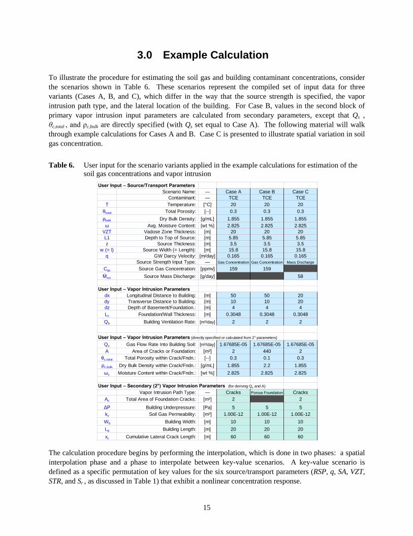
To illustrate the procedure for estimating the soil gas and building contaminant concentrations, consider

the scenarios shown in Table 6. These scenarios represent the compiled set of input data for three

variants (Cases A, B, and C), which differ in the way that the source strength is specified, the vapor

intrusion path type, and the lateral location of the building. For Case B, values in the second block of

primary vapor intrusion input parameters are calculated from secondary parameters, except that Qs ,

θc,total , and ρc,bulk are directly specified (with Qs set equal to Case A). The following material will walk

through example calculations for Cases A and B. Case C is presented to illustrate spatial variation in soil

gas concentration.

Table 6. User input for the scenario variants applied in the example calculations for estimation of the

soil gas concentrations and vapor intrusion

The calculation procedure begins by performing the interpolation, which is done in two phases: a spatial

interpolation phase and a phase to interpolate between key-value scenarios. A key-value scenario is

defined as a specific permutation of key values for the six source/transport parameters (RSP, q, SA, VZT,

STR, and Sr , as discussed in Table 1) that exhibit a nonlinear concentration response.

User Input – Source/Transport Parameters

Scenario Name: — Case A Case B Case C

Contaminant: — TCE TCE TCE

T Temperature: [°C] 20 20 20

θtotal Total Porosity: [--] 0.3 0.3 0.3

ρbulk Dry Bulk Density: [g/mL] 1.855 1.855 1.855

ω Avg. Moisture Content: [wt %] 2.825 2.825 2.825

VZT Vadose Zone Thickness: [m] 20 20 20

L1 Depth to Top of Source: [m] 5.85 5.85 5.85

z Source Thickness: [m] 3.5 3.5 3.5

w (= l) Source Width (= Length): [m] 15.8 15.8 15.8

q GW Darcy Velocity: [m/day] 0.165 0.165 0.165

Source Strength Input Type: — Gas Concentration Gas Concentration Mass Discharge

Cgs Source Gas Concentration: [ppmv] 159 159

Ṁsrc Source Mass Discharge: [g/day] 58

User Input – Vapor Intrusion Parameters

dx Longitudinal Distance to Building: [m] 50 50 20

dy Transverse Distance to Building: [m] 10 10 20

dz Depth of Basement/Foundation.: [m] 4 4 4

Lc Foundation/Wall Thickness: [m] 0.3048 0.3048 0.3048

Qb Building Ventilation Rate: [m³/day] 2 2 2

User Input – Vapor Intrusion Parameters (directly specified or calculated from 2° parameters)

Qs Gas Flow Rate Into Building Soil: [m³/day] 1.67685E-05 1.67685E-05 1.67685E-05

A Area of Cracks or Foundation: [m²] 2 440 2

θc,total Total Porosity within Crack/Fndn.: [--] 0.3 0.1 0.3

ρc,bulk Dry Bulk Density within Crack/Fndn.: [g/mL] 1.855 2.2 1.855

ωc Moisture Content within Crack/Fndn.: [wt %] 2.825 2.825 2.825

User Input – Secondary (2°) Vapor Intrusion Parameters (for deriving Qs and A)

Vapor Intrusion Path Type: — Cracks Porous Foundation Cracks

Ac Total Area of Foundation Cracks: [m²] 2 2

ΔP Building Underpressure: [Pa] 5 5 5

kv Soil Gas Permeability: [m²] 1.00E-12 1.00E-12 1.00E-12

Wb Building Width: [m] 10 10 10

Lb Building Length: [m] 20 20 20

xc Cumulative Lateral Crack Length: [m] 60 60 60

16

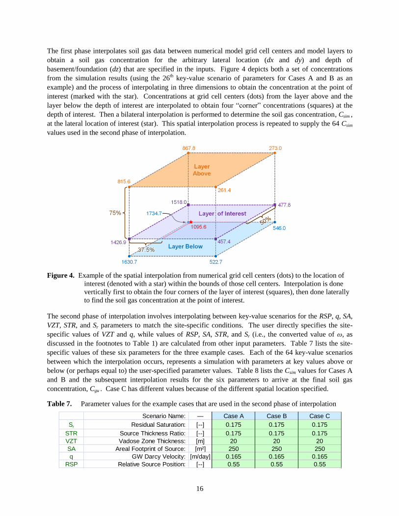
The first phase interpolates soil gas data between numerical model grid cell centers and model layers to

obtain a soil gas concentration for the arbitrary lateral location (dx and dy) and depth of

basement/foundation (dz) that are specified in the inputs. Figure 4 depicts both a set of concentrations

from the simulation results (using the 26th key-value scenario of parameters for Cases A and B as an

example) and the process of interpolating in three dimensions to obtain the concentration at the point of

interest (marked with the star). Concentrations at grid cell centers (dots) from the layer above and the

layer below the depth of interest are interpolated to obtain four “corner” concentrations (squares) at the

depth of interest. Then a bilateral interpolation is performed to determine the soil gas concentration, Csim ,

at the lateral location of interest (star). This spatial interpolation process is repeated to supply the 64 Csim

values used in the second phase of interpolation.

Figure 4. Example of the spatial interpolation from numerical grid cell centers (dots) to the location of

interest (denoted with a star) within the bounds of those cell centers. Interpolation is done

vertically first to obtain the four corners of the layer of interest (squares), then done laterally

to find the soil gas concentration at the point of interest.

The second phase of interpolation involves interpolating between key-value scenarios for the RSP, q, SA,

VZT, STR, and Sr parameters to match the site-specific conditions. The user directly specifies the site-

specific values of VZT and q, while values of RSP, SA, STR, and Sr (i.e., the converted value of ω, as

discussed in the footnotes to Table 1) are calculated from other input parameters. Table 7 lists the site-

specific values of these six parameters for the three example cases. Each of the 64 key-value scenarios

between which the interpolation occurs, represents a simulation with parameters at key values above or

below (or perhaps equal to) the user-specified parameter values. Table 8 lists the Csim values for Cases A

and B and the subsequent interpolation results for the six parameters to arrive at the final soil gas

concentration, Cgu . Case C has different values because of the different spatial location specified.

Table 7. Parameter values for the example cases that are used in the second phase of interpolation

Scenario Name: — Case A Case B Case C

Sr Residual Saturation: [--] 0.175 0.175 0.175

STR Source Thickness Ratio: [--] 0.175 0.175 0.175

VZT Vadose Zone Thickness: [m] 20 20 20

SA Areal Footprint of Source: [m²] 250 250 250

q GW Darcy Velocity: [m/day] 0.165 0.165 0.165

RSP Relative Source Position: [--] 0.55 0.55 0.55

17

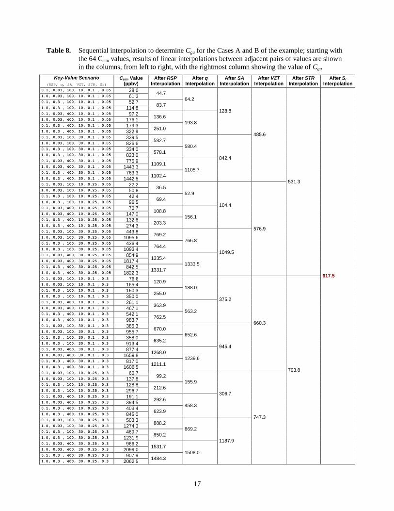
Table 8. Sequential interpolation to determine Cgu for the Cases A and B of the example; starting with

the 64 Csim values, results of linear interpolations between adjacent pairs of values are shown

in the columns, from left to right, with the rightmost column showing the value of Cgu

Key-Value Scenario

(RSP, q, SA, VZT, STR, Sr)

Csim Value (ppbv)

After RSP Interpolation

After q Interpolation

After SA Interpolation

After VZT Interpolation

After STR Interpolation

After Sr Interpolation

0.1, 0.03, 100, 10, 0.1 , 0.05 28.0 44.7

64.2

128.8

485.6

531.3

617.5

1.0, 0.03, 100, 10, 0.1 , 0.05 61.3 0.1, 0.3 , 100, 10, 0.1 , 0.05 52.7

83.7 1.0, 0.3 , 100, 10, 0.1 , 0.05 114.8 0.1, 0.03, 400, 10, 0.1 , 0.05 97.2

136.6

193.8 1.0, 0.03, 400, 10, 0.1 , 0.05 176.1 0.1, 0.3 , 400, 10, 0.1 , 0.05 179.3

251.0 1.0, 0.3 , 400, 10, 0.1 , 0.05 322.9 0.1, 0.03, 100, 30, 0.1 , 0.05 339.5

582.7

580.4

842.4

1.0, 0.03, 100, 30, 0.1 , 0.05 826.6 0.1, 0.3 , 100, 30, 0.1 , 0.05 334.0

578.1 1.0, 0.3 , 100, 30, 0.1 , 0.05 823.0 0.1, 0.03, 400, 30, 0.1 , 0.05 775.9

1109.1

1105.7 1.0, 0.03, 400, 30, 0.1 , 0.05 1443.3 0.1, 0.3 , 400, 30, 0.1 , 0.05 763.3

1102.4 1.0, 0.3 , 400, 30, 0.1 , 0.05 1442.5 0.1, 0.03, 100, 10, 0.25, 0.05 22.2

36.5

52.9

104.4

576.9

1.0, 0.03, 100, 10, 0.25, 0.05 50.8 0.1, 0.3 , 100, 10, 0.25, 0.05 42.4

69.4 1.0, 0.3 , 100, 10, 0.25, 0.05 96.5 0.1, 0.03, 400, 10, 0.25, 0.05 70.7

108.8

156.1 1.0, 0.03, 400, 10, 0.25, 0.05 147.0 0.1, 0.3 , 400, 10, 0.25, 0.05 132.6

203.3 1.0, 0.3 , 400, 10, 0.25, 0.05 274.3 0.1, 0.03, 100, 30, 0.25, 0.05 443.8

769.2

766.8

1049.5

1.0, 0.03, 100, 30, 0.25, 0.05 1095.6 0.1, 0.3 , 100, 30, 0.25, 0.05 436.4

764.4 1.0, 0.3 , 100, 30, 0.25, 0.05 1093.4 0.1, 0.03, 400, 30, 0.25, 0.05 854.9

1335.4

1333.5 1.0, 0.03, 400, 30, 0.25, 0.05 1817.4 0.1, 0.3 , 400, 30, 0.25, 0.05 842.5

1331.7 1.0, 0.3 , 400, 30, 0.25, 0.05 1822.3 0.1, 0.03, 100, 10, 0.1 , 0.3 76.6

120.9

188.0

375.2

660.3

703.8

1.0, 0.03, 100, 10, 0.1 , 0.3 165.4 0.1, 0.3 , 100, 10, 0.1 , 0.3 160.3

255.0 1.0, 0.3 , 100, 10, 0.1 , 0.3 350.0 0.1, 0.03, 400, 10, 0.1 , 0.3 261.1

363.9

563.2 1.0, 0.03, 400, 10, 0.1 , 0.3 467.1 0.1, 0.3 , 400, 10, 0.1 , 0.3 542.1

762.5 1.0, 0.3 , 400, 10, 0.1 , 0.3 983.7 0.1, 0.03, 100, 30, 0.1 , 0.3 385.3

670.0

652.6

945.4

1.0, 0.03, 100, 30, 0.1 , 0.3 955.7 0.1, 0.3 , 100, 30, 0.1 , 0.3 358.0

635.2 1.0, 0.3 , 100, 30, 0.1 , 0.3 913.4 0.1, 0.03, 400, 30, 0.1 , 0.3 877.4

1268.0

1239.6 1.0, 0.03, 400, 30, 0.1 , 0.3 1659.8 0.1, 0.3 , 400, 30, 0.1 , 0.3 817.0

1211.1 1.0, 0.3 , 400, 30, 0.1 , 0.3 1606.5 0.1, 0.03, 100, 10, 0.25, 0.3 60.7

99.2

155.9

306.7

747.3

1.0, 0.03, 100, 10, 0.25, 0.3 137.8 0.1, 0.3 , 100, 10, 0.25, 0.3 128.8

212.6 1.0, 0.3 , 100, 10, 0.25, 0.3 296.7 0.1, 0.03, 400, 10, 0.25, 0.3 191.1

292.6

458.3 1.0, 0.03, 400, 10, 0.25, 0.3 394.5 0.1, 0.3 , 400, 10, 0.25, 0.3 403.4

623.9 1.0, 0.3 , 400, 10, 0.25, 0.3 845.0 0.1, 0.03, 100, 30, 0.25, 0.3 503.3

888.2

869.2

1187.9

1.0, 0.03, 100, 30, 0.25, 0.3 1274.3 0.1, 0.3 , 100, 30, 0.25, 0.3 469.7

850.2 1.0, 0.3 , 100, 30, 0.25, 0.3 1231.9 0.1, 0.03, 400, 30, 0.25, 0.3 966.2

1531.7

1508.0 1.0, 0.03, 400, 30, 0.25, 0.3 2099.0 0.1, 0.3 , 400, 30, 0.25, 0.3 907.9

1484.3 1.0, 0.3 , 400, 30, 0.25, 0.3 2062.5

18

The first column of Table 8 lists the Csim values from the spatial interpolation for Cases A and B. Each

subsequent column is determined by applying the linear interpolation of Equation 1 to adjacent values.

The key RSP values (Table 1) are 0.1 and 1.0, because the site-specific RSP value is 0.55 (Table 7). The

first pair of Csim values in Table 8 corresponds to those two key values of RSP (for the same key values of

q, SA, VZT, STR, and Sr), so interpolation for RSP can be applied as:

7440280283611001

10550..)..(

..

.. ppbv

This same interpolation process is performed for the remaining pairs of Csim values to get the intermediate

interpolation results in the second column of Table 8. Pairs of values from the second column are then

interpolated to obtain concentration values for the user-specified q value of 0.165 m/day (Table 7). The

key q values (Table 1) above and below the site-specific q are 0.03 and 0.3 m/day. The interpolation of

the first pair of concentrations in the second column thus gives:

26478378374403030

0301650..)..(

..

.. ppbv

This process continues in the same fashion for pairs of values with interpolation between key values to

the site-specific conditions for the q, SA, VZT, STR, and Sr parameters. The results of these sequential

linear interpolations are shown in Table 8, with the final interpolation providing the Cgu value of 617.5

ppbv (for Cases A and B).

For Case C of the example, interpolation is required to determine the source mass discharge, Ṁsim ,

corresponding to the site-specific parameter values. This value is used in the scaling process.

Interpolation to determine Ṁsim does not involve the first phase of spatial interpolation (because it pertains

to the defined source), but does involve the second phase to interpolate to the site-specific conditions for

the RSP, q, SA, VZT, STR, and Sr parameters in a process parallel to that shown in Table 8. The initial

values of mass discharge, from which the 64 values are drawn, are tabulated in the VIETUS software (see

the SVEET documentation [Truex et al., 2013] for a list of all mass discharge values). For Case C, the

resultant Ṁsim is 58.3 g/day and the Cgu value is 1425.9 ppmv.

Once Cgu (and Ṁsim , if needed) are determined, the next step is to apply scaling factors for the two

parameters (Henry’s Law Constant and source strength) where concentration exhibits a linear response.

The vapor pressure and solubility for trichloroethene at 20 °C are calculated using contaminant-specific

correlations in Equations 2 and 3 (with conversion of solubility to mole fraction based on Equation 5):

Pvap = 10[6.87981 – 1157.83 / (20.0 + 202.58)]

= 47.6376 mm Hg

xp = [1.4049 – 0.0082223·(20.0 + 273.15) + 0.000013218·(20.0 + 273.15)²] / 100 = 0.13045

x = (0.13045 / 100)·(18.01528 / 131.387) = 1.7886×10-4

These results are used with Equation 6 to obtain the dimensionless value for the Henry’s Law constant:

263.0760

1

1000

1

15.29308205746.09982.0

18.01528

00017886.0

6376.47

19

For Cases A and B of the example, Equation 7 is applied to obtain the final estimated soil gas

contaminant concentration, Cg , at the specified location beneath the building foundation. For Case C,

Equation 8 is applied to obtain Cg because the source strength is specified as a mass discharge. These

final calculations give the following results:

ppmv20900159

0159

2630

8905617BACases

.

.

.

..:&

ppmv4798358

58

2630

89091425CCase

..

..:

Given the soil gas concentration beneath the building foundations, the final step is to generate the

estimate of the contaminant concentration in the building due to vapor intrusion. The diffusion

coefficient in air for TCE at 20°C is calculated with the correlation formula of Equation 11 and associated

constants in Table 5:

Da = -4.127E-2 + (2.658E-4)(293.15) + (5.5704E-7)(293.15)² = 0.0845 cm²/s = 0.73025 m²/day

The diffusion coefficient through cracks in the foundation (Cases A and C) are then calculated with

Equation 10:

daym0772030

23770730250D23770

99820100

22825230 2

2cgc

310

/..

).(..

.

...,

The diffusion coefficient for a porous foundation (Case B) is calculated in the same way, giving a value

of 0.0013 m²/day when the appropriate values are used with Equation 10.

The area through which vapor intrusion occurs is taken to be the specified area of the cracks (2 m²) for

Cases A and C, and the total surface area of the subsurface foundations for Case B:

A = 2·Wb·dz + 2·Lb·dz + Wb·Lb = 2·10·4 + 2·20·4 + 10·20 = 440 m²

The flow rate of gas from the soil into the building can be estimated (for Cases A and C, but also used for

Case B) with Equation 12 as:

daym449126044

60

101072

0152Q 3

10

-12

s /.)ln()ln(.

Having defined all key values, Equation 9 can be applied to determine the estimate for the contaminant

concentration in the building. First calculating the exponential term for the example cases:

17.44207720

304804491

AD

LQ

c

cs

)().(

).().(exp for Cases A and C

= 2.14 for Case B (using Dc = 0.0013 and A = 440)

20

Then, completing the calculation for each separate example case, the contaminant concentration in the

building is estimated to be:

ppmv15394491244172

441720904491Cb

..

.. for Case A

ppmv1738449121422

14220904491Cb

..

.. for Case B

ppmv35314491244172

441747984491Cb

..

.. for Case C

21

4.0 VIETUS User Guide

For user convenience, the calculational procedure described in Section 2.0 for estimating a soil gas

contaminant concentration in the vadose zone and the associated vapor intrusion concentration has been

implemented in a spreadsheet software tool. The VIETUS software allows the user to easily enter data

and calculate the estimated soil gas and building concentrations for one or more scenarios conforming to

the generalized conceptual model described in Section 2.0. The system requirements, installation, user

interface, and application of the VIETUS software are described in the sections below.

4.1 System Requirements

The following hardware and software are required to use the VIETUS software:

Personal computer based on Intel® IA-32 or Intel® 64 processor architectures,

Microsoft® Windows

® XP or Microsoft

® Windows

® 7 operating system,

Microsoft® Excel

® 2007 or Excel

® 2010

The VIETUS software should also work with Windows® 8 and Excel

® 2013, but neither has specifically

been tested. Use of the operating system/Excel versions specified above is encouraged; otherwise the

user is advised to carefully check results for validity.

4.2 Installing and Starting VIETUS

The VIETUS software is distributed as a compressed file (in ‘zip’ format) containing four files. The files

consist of an Excel workbook file, two text files, and an electronic version of this report. These files may

be extracted into any convenient directory, but all three files must be in the same directory (otherwise

VIETUS will not run). Note that, when uncompressed, the three files will occupy a total of about 90 MB

of hard-disk space.

To run VIETUS, simply open the Excel workbook file like you would any other Excel workbook. It is

recommended that you manage the use of the VIETUS software for different scenarios/projects by

changing the VIETUS workbook file name (either by copying and renaming the original VIETUS file or

by performing a “SaveAs…” operation from within Excel).

The VIETUS workbook relies on user-defined functions (i.e., macros) to perform certain calculations, so

macros must be enabled for calculations to work properly. The user should select the “Enable Macros”

option when opening a VIETUS workbook. If not presented with an option to enable macros, the user

can try closing and re-opening the file or the user may need to alter the macro security settings within

Excel. Security options in recent versions of Excel are found under the name of “Macro Security” or

“Trust Center” (depending on the version of Excel). Security options can be set to prompt/notify the user

to confirm whether macros should be enabled (or not) for a specific workbook.

22

4.3 Description of the VIETUS Workbook

The VIETUS Excel workbook contains three worksheets available to the user, including a software

notice, the “HLC” worksheet, and the “VIETUS” worksheet. The software notice worksheet provides

important notification/disclaimer text relevant to the use of the software. The “HLC” and “VIETUS”

worksheets are described below.

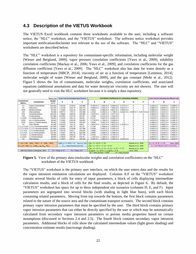
The “HLC” worksheet is a repository for contaminant-specific information, including molecular weight

[Wieser and Berglund, 2009], vapor pressure correlation coefficients [Yaws et al., 2009], solubility

correlation coefficients [Mackay et al., 2006; Yaws et al., 2009], and correlation coefficients for the gas

diffusion coefficient [Yaws et al., 2009]. The “HLC” worksheet also has data for water density as a

function of temperature [HBCP, 2014], viscosity of air as a function of temperature [Lemmon, 2014],

molecular weight of water [Wieser and Berglund, 2009], and the gas constant [Mohr et al., 2012].

Figure 5 shows the list of contaminants, molecular weights, correlation coefficients, and associated

equations (additional annotations and data for water density/air viscosity are not shown). The user will

not generally need to visit the HLC worksheet because it is simply a data repository.

Figure 5. View of the primary data (molecular weights and correlation coefficients) on the “HLC”

worksheet of the VIETUS workbook

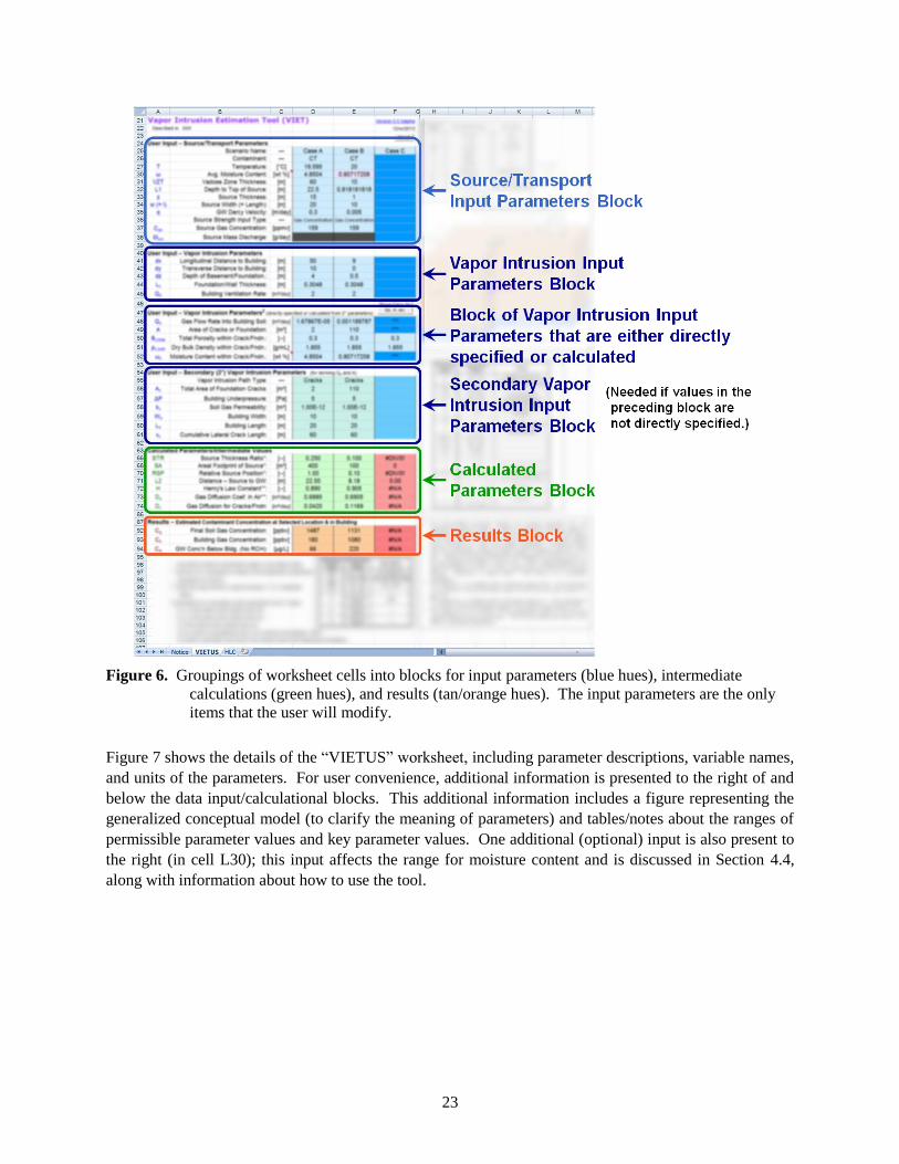
The “VIETUS” worksheet is the primary user interface, on which the user enters data and the results for

the vapor intrusion estimation calculations are displayed. Columns A:F on the “VIETUS” worksheet

contain several blocks of cells for entry of input parameters, a block of cells displaying intermediate

calculation results, and a block of cells for the final results, as depicted in Figure 6. By default, the

“VIETUS” worksheet has space for up to three independent site scenarios (columns D, E, and F). Input

parameters are segregated into several blocks (with shading in light blue hues), with each block

containing related parameters. Moving from top towards the bottom, the first block contains parameters

related to the nature of the source area and the contaminant transport scenario. The second block contains

primary vapor intrusion parameters that must be specified by the user. The third block contains primary

vapor intrusion parameters that can either be directly specified by the user or which may be automatically

calculated from secondary vapor intrusion parameters or porous media properties based on certain

assumptions (discussed in Sections 2.4 and 2.5). The fourth block contains secondary vapor intrusion

parameters. Additional blocks of cells show the calculated intermediate values (light green shading) and

concentration estimate results (tan/orange shading).

Correl. Coef. for Calculating Vapor Pressure Correlation Coefficients for Calculating Solubility Correl. Coef. for Calculating Gas Diffusion Coef.

Contaminant

Abbrev.Contaminant A B C

E

q

n

A B C D E F A B C

CT Carbon Tetrachloride 153.823 7.01144 1278.54 232.888 2 9.7842 E-2 -1.4942 E-3 3.5854 E-5 2.2775 E-7 0 0 -4.1620 E-2 2.5749 E-4 5.3598 E-7

CF Chloroform 119.378 7.11148 1232.79 230.213 2 9.9500 E-1 -1.0531 E-2 7.9819 E-5 6.6431 E-7 0 0 -4.9960 E-2 2.8829 E-4 5.9407 E-7

DCM Dichloromethane 84.933 7.11464 1152.41 232.442 2 1.9610 -4.4883 E-2 8.6617 E-4 4.9463 E-6 0 0 -5.6860 E-2 3.3534 E-4 6.8151 E-7

CM Chloromethane 50.488 6.99771 870.17 235.586 3 1.4019 -6.3562 E-2 1.7198 E-3 -2.8262 E-5 2.5268 E-7 -9.3470 E-10 -6.9250 E-2 4.2133 E-4 8.2225 E-7

PCE Tetrachloroethene 165.833 7.06892 1458.45 226.986 1 2.6479 E-1 -1.5487 E-3 2.4477 E-6 0 0 0 -3.6840 E-2 2.3847 E-4 5.1123 E-7

TCE Trichloroethene 131.388 6.87981 1157.83 202.58 1 1.4049 -8.2223 E-3 1.3218 E-5 0 0 0 -4.1270 E-2 2.6580 E-4 5.5704 E-7

1,1-DCE 1,1-Dichloroethene 96.943 7.21678 1181.12 240.84 1 6.2741 -3.8257 E-2 6.0461 E-5 0 0 0 -4.5030 E-2 2.9721 E-4 6.0085 E-7

cDCE cis-1,2-Dichloroethene 96.943 7.21953 1290.28 236.887 1 2.7735 E+1 -1.7832 E-1 2.9328 E-4 0 0 0 -4.6220 E-2 3.0091 E-4 6.1981 E-7

tDCE trans-1,2-Dichloroethene 96.943 7.21356 1244.35 239.497 1 7.8039 -4.5457 E-2 6.9676 E-4 0 0 0 -4.6380 E-2 3.0373 E-4 6.2044 E-7

VC Vinyl Chloride 62.498 6.91423 911.15 239.8 4 -4.6670 E+2 1.3479 E+4 1.8523 E+2 -1.3236 E-1 0 0 -5.4240 E-2 3.6658 E-4 7.2028 E-7

1,1,1,2-TeCA 1,1,1,2-Tetrachloroethane 167.849 7.03897 1467.16 222.34 1 2.1790 -1.3966 E-3 2.9328 E-5 0 0 0 -3.6290 E-2 2.2950 E-4 4.9507 E-7

1,1,2,2-TeCA 1,1,2,2-Tetrachloroethane 167.849 6.91043 1378.88 197.086 1 4.8798 -3.0937 E-3 5.2051 E-5 0 0 0 -4.0420 E-2 2.2899 E-4 4.9882 E-7

1,1,1-TCA 1,1,1-Trichloroethane 133.404 7.00718 1253.2 229.624 1 1.0909 -6.5278 E-3 1.1075 E-5 0 0 0 -4.5040 E-2 2.5770 E-4 5.3553 E-7

1,1,2-TCA 1,1,2-Trichloroethane 133.404 7.14357 1457.65 228.099 1 2.8980 -1.8585 E-2 3.4896 E-5 0 0 0 -4.4400 E-2 2.5339 E-4 5.4055 E-7

1,1-DCA 1,1-Dichloroethane 98.959 7.18316 1269.43 237.755 1 9.4136 -5.7249 E-2 9.1784 E-5 0 0 0 -4.7450 E-2 2.8979 E-4 5.9566 E-7

1,2-DCA 1,2-Dichloroethane 98.959 7.29525 1407.85 235.48 1 1.7915 E+1 -1.1684 E-1 2.0003 E-4 0 0 0 -4.8920 E-2 2.8847 E-4 6.0315 E-7

CE Chloroethane 64.514 7.13047 1097.6 246.009 2 5.8420 E-1 -1.6863 E-3 9.3949 E-5 -2.5316 E-6 0 0 -5.5930 E-2 3.4520 E-4 6.8934 E-7

<dummy row>

x = (xp / 100) · (MWw / MWi) = xf · (MWw / MWi) Log(Pvap) = A - B/(Tc + C) Yaws et al., 2009 1: xp = A + B·Tk + C·Tk² Mackay et al., 2006 Da = A + B·Tk + C·Tk² Yaws, 2003

H = [ (P / 760) / x ] · [ MWw / (ρw·Rgas·Tk) ] Pv ap = Vapor Pressure (mm Hg) 2: xp = A + B·Tc + C·Tc² + D·Tc³ Mackay et al., 2006 Da = Gas Diffusion Coeff. in Air (cm²/s)

3: xp = A + B·Tc + C·Tc² + D·Tc³ + E·Tc4 + F·Tc

5Mackay et al., 2006

MW from Wieser & Berglund, 2009 Tc = Temp. in °C Tk = Temp. in K 4: Log(xf) = A + B/Tk + C·Log(Tk) + D·Tk Yaws, 2003

xp = mass fraction × 100% xf = mass fraction

Molecular

Weight

(g/mol)

23

Figure 6. Groupings of worksheet cells into blocks for input parameters (blue hues), intermediate

calculations (green hues), and results (tan/orange hues). The input parameters are the only

items that the user will modify.

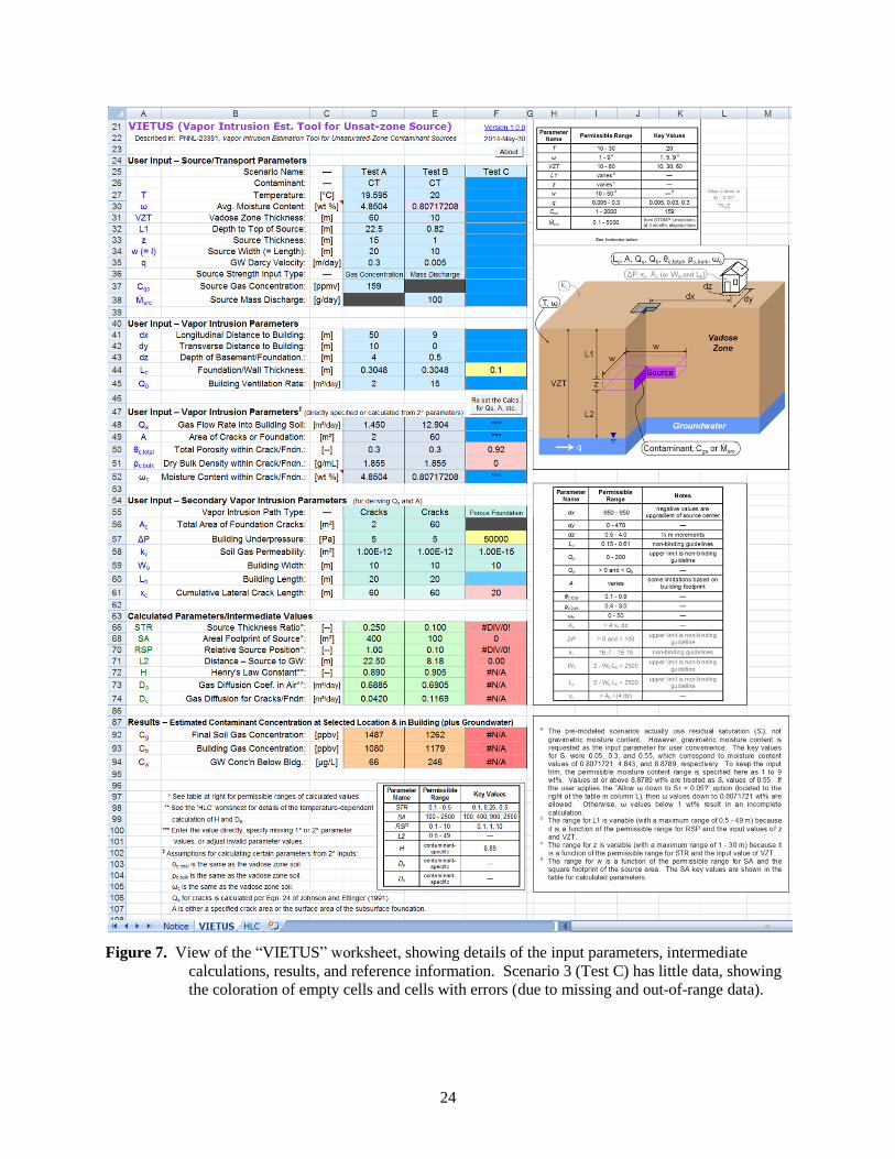
Figure 7 shows the details of the “VIETUS” worksheet, including parameter descriptions, variable names,

and units of the parameters. For user convenience, additional information is presented to the right of and

below the data input/calculational blocks. This additional information includes a figure representing the

generalized conceptual model (to clarify the meaning of parameters) and tables/notes about the ranges of

permissible parameter values and key parameter values. One additional (optional) input is also present to

the right (in cell L30); this input affects the range for moisture content and is discussed in Section 4.4,

along with information about how to use the tool.

24

Figure 7. View of the “VIETUS” worksheet, showing details of the input parameters, intermediate

calculations, results, and reference information. Scenario 3 (Test C) has little data, showing

the coloration of empty cells and cells with errors (due to missing and out-of-range data).

25

4.4 Using the Software

The VIETUS software is implemented as an Excel workbook, thus the standard features of Excel apply—

that is, the user should be familiar with how to operate Excel. Once a VIETUS workbook is opened (and

macros are enabled, as discussed in Section 4.2), performing calculations is as simple as entering the data

required to describe the site of interest using the context of the generalized conceptual site model (Section

2.1). On input of valid data, results are available immediately. The VIETUS workbook includes two

features to help maintain the integrity of the calculations. The associated macro code is locked for

viewing or editing. Also, the worksheets are protected and data entry is only allowed in appropriate data

input cells.

For most items, data entry consists of entering parameter values for a particular scenario (in columns D,

E, and/or F). Empty data input cells are all shaded a (darker) blue color, with the shading color changing

upon entry of data (to either a light blue/aqua, light yellow, or light red, as shown in Figure 7). Light red

shading of an input parameter value or an intermediate calculation value indicates that invalid data has

been entered for one or more parameters. Light yellow shading indicates that a recommended bound has

been exceeded. The primary cause for errors is likely to be data values outside the permissible ranges or

values that are inconsistent with each other, such as a source thickness that is inconsistent with the vadose

zone thickness and/or L1 parameter. The tables of permissible ranges and a diagram of the generalized

conceptual site model are included directly on the worksheet to help the user identify issues with

improper input data.

For the contaminant name, source strength input type, depth of basement/foundation, and vapor intrusion

path type inputs, a selection list is provided to ensure entry of valid data. The selection list is activated by

selecting the input cell on the spreadsheet then clicking on the arrow button that appears. The selection of

the source strength input type modifies the requested input data to be either source gas concentration or

source mass discharge, while graying out the unused parameter. Similarly, the selection of a porous

foundation as the vapor intrusion path type causes the total area of foundation cracks parameter to be

grayed out.

An optional input (“Allow ω down to Sr = 0.05?”) exists in cell L30 to indicate whether soil moisture (ω)

values down to the equivalent residual saturation (Sr) of 0.05 can be input (true) or not (false). This

effectively alters the permissible range as described in Section 2.1 (and Figure 3). Soil moisture values

that are below the listed lower range and those that are above the maximum residual saturation are

colored light lavender to indicate that special circumstances are in effect.

The contaminant source/transport input parameters are relatively straightforward, but the vapor intrusion

input parameters encompass three blocks of related inputs, as discussed in Section 4.3. The first block

consists of key parameters that must be specified by the user. The second block consists of key

parameters for which a formula is provided to calculate the value (based on secondary input parameters or

porous media properties). The third block consists of the optional secondary input parameters. The user

has two options for setting the values of the second block of vapor intrusion input parameters. The user

can enter the input parameter values directly (and leave the secondary vapor intrusion input parameters

unspecified). Or the user can specify the secondary vapor intrusion input parameters and allow the

second block of vapor intrusion input parameters to be calculated automatically based on the approaches

and assumptions discussed in Sections 2.4 and 2.5. If the user directly specifies the value for a vapor

intrusion parameter in the second block and later decides to instead use the secondary input parameters to

26

calculate that parameter, the formulas for the second block of vapor intrusion parameters can be re-set by

clicking on the “Reset Calcs…” button at row 46.

The final output consists of the estimated soil vapor gas concentration underneath the building and the

contaminant concentration inside the building due to vapor intrusion. The concentration of contaminant

in the groundwater due to the specified source/site scenario at a location vertically below the specified

point of interest is also shown. This groundwater concentration reflects the average estimated

concentration in the top meter of aquifer (which differs from SVEET, where groundwater concentrations

are averaged over a specified well screen length). The groundwater concentration is provided for user

reference for assessing the results. Sites with groundwater sources or with higher recharge may have

different groundwater concentrations and may need a full site-specific numerical model to assess the

impacts of such conditions.

27

5.0 References

Brennan, R.A., N. Nirmalakhandan, and R.E. Speece. 1998. “Comparison of Predictive Methods for

Henrys Law Coefficients of Organic Chemicals.” Water Res., 32(6):1901-1911.

Chen, F., D.L. Freedman, R.W. Falta, and L.C. Murdoch. 2012. “Henry’s Law Constants of Chlorinated

Solvents at Elevated Temperatures.” Chemosphere, 86(2):156-165.

HBCP. 2014. “Standard Density of Water.” In: CRC Handbook of Chemistry and Physics, 94th Edition

(Internet Version 2014), W. M. Haynes, ed. CRC Press/Taylor and Francis, Boca Raton, Florida.

Johnson, P.C., and R.A. Ettinger. 1991. “Heuristic Model for Predicting the Intrusion Rate of

Contaminant Vapors into Buildings.” Environ. Sci. Technol., 25(8):1445-1452.

Lemmon, E.W. 2014. “Thermophysical Properties of Air.” In: CRC Handbook of Chemistry and

Physics, 94th Edition (Internet Version 2014), W. M. Haynes, ed. CRC Press/Taylor and Francis,

Boca Raton, Florida.

Mackay D, WY Shiu, K Ma, and SC Lee. 2006. Handbook of Physical-Chemical Properties and

Environmental Fate for Organic Chemicals, Second Ed, Volume II, Halogenated Hydrocarbons.

CRC Press, Boca Raton, Florida.

Mohr, P.J., B.N. Taylor, and D.B. Newell. 2012. “CODATA Recommended Values of the Fundamental

Physical Constants: 2010.” J. Phys. Chem. Ref. Data, 41(4):043109.

Nazaroff, W.W. 1988. “Predicting the Rate of 222Rn Entry from Soil into the Basement of a Dwelling

Due to Pressure-Driven Air Flow.” Radiat. Prot. Dosim., 24(1-4):199-202.

Sander, R. 1999. “Modeling Atmospheric Chemistry: Interactions Between Gas-Phase Species and

Liquid Cloud/Aerosol Particles.” Surv. Geophys., 20(1):1-31.

Staudinger, J., and P.V. Roberts. 2001. “A Critical Compilation of Henry’s Law Constant Temperature

Dependence Relations for Organic Compounds in Dilute Aqueous Solutions.” Chemosphere,

44(4):561-576.

Truex, M.J., D.J. Becker, M.A. Simon, M. Oostrom, and A.K. Rice. 2013. Soil Vapor Extraction System

Optimization, Transition, and Closure Guidance. PNNL-21843, Pacific Northwest National

Laboratory, Richland, Washington.

Warneck, P. 2007. “A Review of Henry’s Law Coefficients for Chlorine-Containing C1 and C2

Hydrocarbons.” Chemosphere, 69(3):347-361.

White, M.D., and M. Oostrom. 2006. STOMP Subsurface Transport Over Multiple Phases, Version 4.0,

User's Guide. PNNL-15782, Pacific Northwest National Laboratory, Richland, Washington.

Wieser, M.E., and M. Berglund. 2009. “Atomic Weights of the Elements 2007 (IUPAC Technical

Report).” Pure Appl. Chem., 81(11):2131-2156.

Yaws, C.L. 2003. Yaws’ Handbook of Thermodynamic and Physical Properties of Chemical

Compounds. Knovel, New York. Electronic ISBN 978-1-59124-444-8.

Yaws, C.L., P.K. Narasimhan, and C. Gabbula. 2009. Yaws’ Handbook of Antoine Coefficients for

Vapor Pressure (2nd Electronic Ed.). Knovel, New York. Electronic ISBN 978-1-59124-879-8.

PNNL-23381

Distribution

No. of No. of

Copies Copies

Distr.1

2 Local Distribution (electronic)

Pacific Northwest National Laboratory

MJ Truex K7-73

CD Johnson K7-73